Numerical Techniques of Natural Circulation: History and Background Juan Carlos Ferreri Autoridad Regulatoria Nuclear, Buenos Aires, Argentina Course on Natural Circulation Phenomena and Modelling in Water-cooled Nuclear Reactors
Transcript
Numerical Techniques of Natural Circulation: History
and Background
Juan Carlos FerreriAutoridad Regulatoria Nuclear, Buenos Aires, Argentina
Course on Natural Circulation Phenomena and Modelling in Water-cooled Nuclear ReactorsICTP, Trieste, Italy, 25 to 29 June, 2007
2
ICTP, 2007
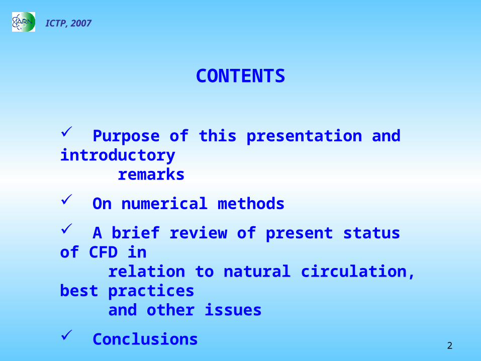
CONTENTS
Purpose of this presentation and introductory remarks
On numerical methods
A brief review of present status of CFD in relation to natural circulation, best practices and other issues
Conclusions
3
ICTP, 2007
PURPOSE OF THIS PRESENTATION
a. There is plenty of consolidated literature and concepts on numerical methods since 50 years ago.
b. CFD is not a new activity in relation to NC and the thermal hydraulics of Nuclear Safety
c. Many outstanding people contributed to this subject in the last five decades
This presentation is aimed at considering several aspects of Numerical Techniques giving the background to the computation of Fluid Dynamics as applied to the Computational Fluid Dynamics (CFD) of Natural Circulation (NC). It will be shown that:
4
ICTP, 2007
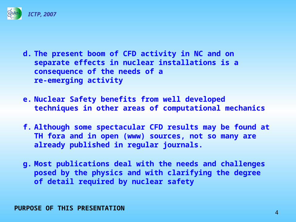
d. The present boom of CFD activity in NC and on separate effects in nuclear installations is a consequence of the needs of a re-emerging activity
e. Nuclear Safety benefits from well developed techniques in other areas of computational mechanics
f. Although some spectacular CFD results may be found at TH fora and in open (www) sources, not so many are already published in regular journals.
g. Most publications deal with the needs and challenges posed by the physics and with clarifying the degree of detail required by nuclear safety
PURPOSE OF THIS PRESENTATION
5
ICTP, 2007
Two possible definitions in this context:
• A numerical technique is an incremental (or discrete) way of representing a differential equation (that is part of a physical model in NC)
• Computational Fluid Dynamics is a discipline that allows solving conservation equations using adequate discrete representations at a desired level of resolution, implying more than a numerical technique
INTRODUCTORY REMARKS
6
ICTP, 2007
INTRODUCTORY REMARKS
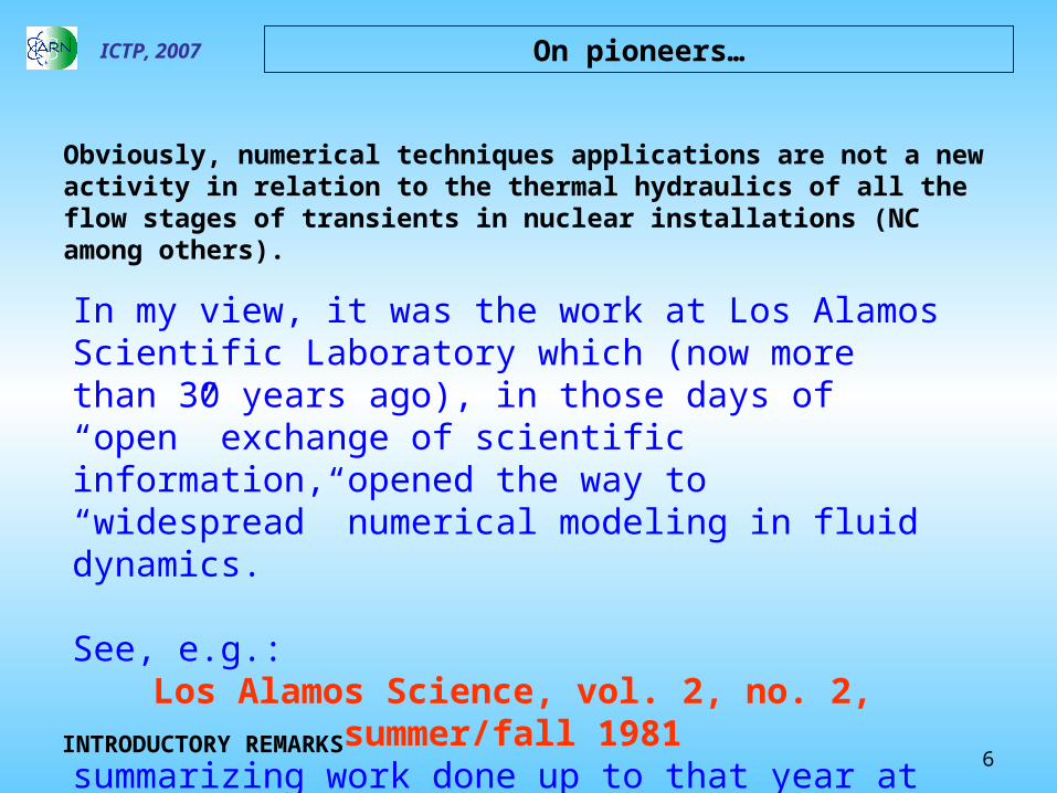
Obviously, numerical techniques applications are not a new activity in relation to the thermal hydraulics of all the flow stages of transients in nuclear installations (NC among others).
In my view, it was the work at Los Alamos Scientific Laboratory which (now more than 30 years ago), in those days of “open” exchange of scientific information, opened the way to “widespread” numerical modeling in fluid dynamics.
See, e.g.:Los Alamos Science, vol. 2, no. 2, summer/fall 1981
summarizing work done up to that year at LANL
On pioneers…
7
ICTP, 2007
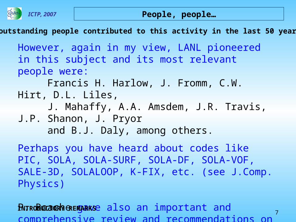
Many outstanding people contributed to this activity in the last 50 years...
However, again in my view, LANL pioneered in this subject and its most relevant people were: Francis H. Harlow, J. Fromm, C.W. Hirt, D.L. Liles, J. Mahaffy, A.A. Amsdem, J.R. Travis, J.P. Shanon, J. Pryor and B.J. Daly, among others.
Perhaps you have heard about codes like PIC, SOLA, SOLA-SURF, SOLA-DF, SOLA-VOF, SALE-3D, SOLALOOP, K-FIX, etc. (see J.Comp. Physics)
P. Roache gave also an important and comprehensive review and recommendations on numerical techniques and CFD by 1972. People at LLNL also contributed significantly
INTRODUCTORY REMARKS
People, people…
8
ICTP, 2007
Other people pioneered in Europe, like B. Spalding, M. Wolfshtein, S. Patankar at Imperial College, R. Peiret at ONERA and many others.
I will just mention some people that contributed to the development from the numerical analysis side...
…because the list is too long, but the names of R. Courant, K.O. Friedrichs, D. Hilbert, J. von Neumann, P.D. Lax, R.D. Richtmyer, G.I. Marchuk (in Russia) and W.F. Ames should, at least, be mentioned.
INTRODUCTORY REMARKS
People, people…
9
ICTP, 2007
The Drift-Flux theory of two-phase flow, as developed by Zuber and Findlay and by M. Ishii in his book, was the physical two-phase fluid model that allowed generating results of Nuclear Safety significance through its implementation in the TRAC code and other hydrodynamics codes at LASL.
Many other people contributed significantly in this field, like J.M. Delhaye, R. Lahey, M. Giot, F.H Moody, G.B. Wallis, R.E. Henry, J.A. Bouré, D.C. Groeneveld, G. Yadigaroglu and simply too many others to be cited here…
INTRODUCTORY REMARKS
People, people…
10
ICTP, 2007
• “In as much as we can simulate reality, we can use the computer to make predictions about what will occur in a certain set of circumstances.
• Finite-difference techniques can create an artificial laboratory for examining situations which would be impossible to observe otherwise, but we must always remain critical of our results.
• Finite-differencing can be an extremely powerful tool, but only when it is firmly set in a basis of physical meaning. In order for a finite-difference code to be successful, we must start from the beginning, dealing with simple cases and examining our logic each step of the way.”
Reference: E. Scannapieco and Francis H. Harlow, Introduction to Finite-Difference Methods for Numerical Fluid Dynamics, LA 12984, issued 1995
INTRODUCTORY REMARKS
An appropriate conceptual excerpt…
11
ICTP, 2007
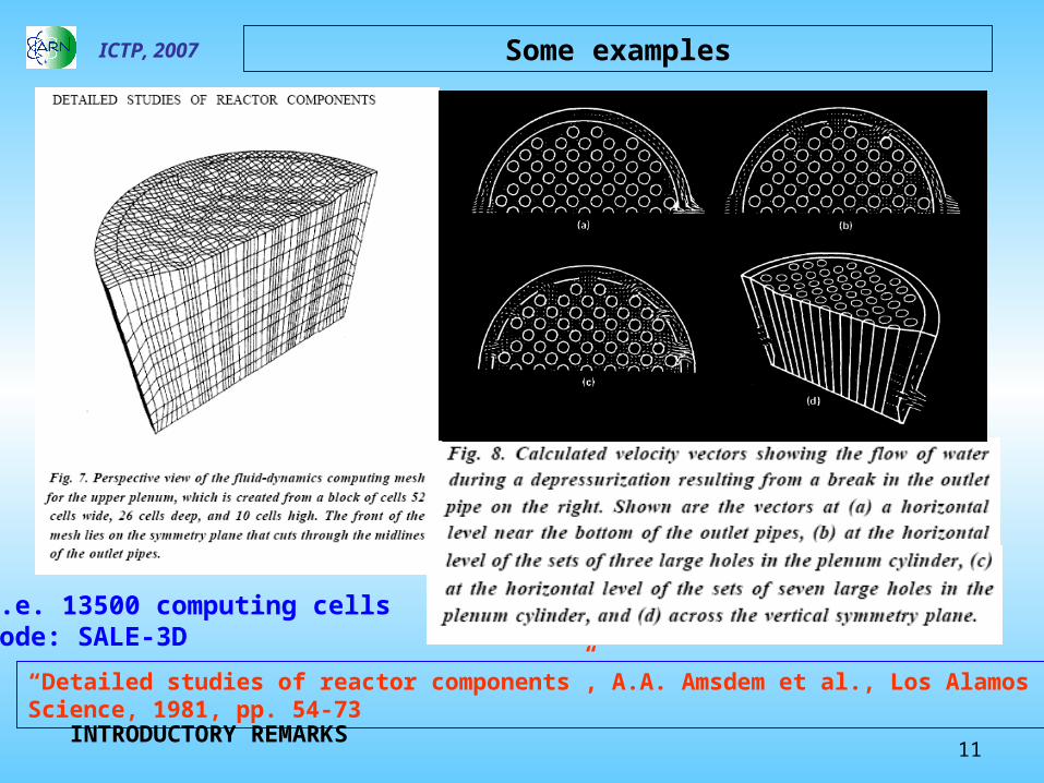
“Detailed studies of reactor components”, A.A. Amsdem et al., Los Alamos Science, 1981, pp. 54-73
i.e. 13500 computing cellscode: SALE-3D
INTRODUCTORY REMARKS
Some examples
12
ICTP, 2007
INTRODUCTORY REMARKS
With far more modest resources we were working too…
B. Martinez and J.C. Ferreri, Lat. American J. of Heat and Mass Transfer, vol. 6, pp. 1-12, 1982 and other references before…
1331 fluid computing cells
code: a SOLA 3D like…
Some examples
13
ICTP, 2007
Understanding the need of making efforts in the appropriate modelling of 1D flows
fluid dynamics
(this seems a somewhat old-fashioned proposal at this time, when multi-
dimensional CFD modelling governs the trends in the analysis of NC and separate effects in Nuclear Safety related issues)
However, let´s make...
INTRODUCTORY REMARKS
A proposal for what follows…
14
ICTP, 2007
Reference: N. Zuber, "Problems in Modeling of Small Break LOCA", NUREG-0724, 1980
For single-phase flows in vertical pipes (or two-phase flows with equal velocities and temperature), the effects of each term in the conservation equations are preserved in model and prototype without any distortion, if one imposes the requirements of: a) Same fluid at equal pressure, properties and enthalpy:
1hh
pp
M
P
M
P
M
P
b) Isochronous phenomena:
mW
W
M
P
M
P
M
P
V
V
They lead to the Power to Volume scaling relations, i.e.:
1M
P t
t
Where m is chosen on the basis of available resources, usually power for the model
A small digression on scaling laws…
INTRODUCTORY REMARKS
15
ICTP, 2007
(This condition is essential to keep equal gravity driving forces, i.e. in the case of Natural Circulation flows).
Then, together with the Power to Volume relations, m SPECIFIES m as the ratio of cross sections. It also implies that velocities ARE equal.
d) Furthermore, frictional effects are equal if:
1M
P ll
1
KA
KA
MC
PC
c) Imposing now equal elevations:
INTRODUCTORY REMARKS
A small digression on scaling laws…
16
ICTP, 2007
From: General Description of the PACTEL Test Facility (VTT/TM/RN-1929, 1998)
Simulates a VVER-440 PWR in Lovisa, FinlandVolumetric scaling 1:305 – Height 1:1 – Loops 3:6
Fuel diameter 1:1 - Power 1 MW
The cause of 30 years delay to 2D/3D?
INTRODUCTORY REMARKS
A small digression on scaling laws…
17
ICTP, 2007
May be because (in my view)...
a) scaling laws “force” to almost 1D integral representations of real life installations, with pre-established flow patterns
b) a huge effort was focused on the development of a representative physical data base (amenable to 1D analysis) and separate effects on the other side (like plume analysis, non-symmetric flow distribution, particular aspects of reactor components behavior, etc.) affordable through detailed computational techniques
c) code assessment for safety analysis also imposed a great effort for 1D
INTRODUCTORY REMARKS
A small digression on scaling laws…
18
ICTP, 2007
...because (in my view)... Cont´d.
d) time scales to solve problems in realistic way (as a compromise between cell Courant number limitation for fast transients using semi-implicit methods and time inaccuracies, i.e. damping, for implicit methods) impose large number of time steps to span long time transients (e.g. in SBLOCAs)
e) ill posedness of the governing equations “precluded” (for some people) search for detailed convergence of solutions, leading to coarse grid computations and stabilization of flow solvers by numerical means
f) computers were not fast, cheap and widely available and not too many were interested in paying for detailed analyses, neither were asking too much for them…
INTRODUCTORY REMARKS
A small digression on scaling laws…
19
ICTP, 2007
INTRODUCTORY REMARKS
...because (in my view) Cont´d.
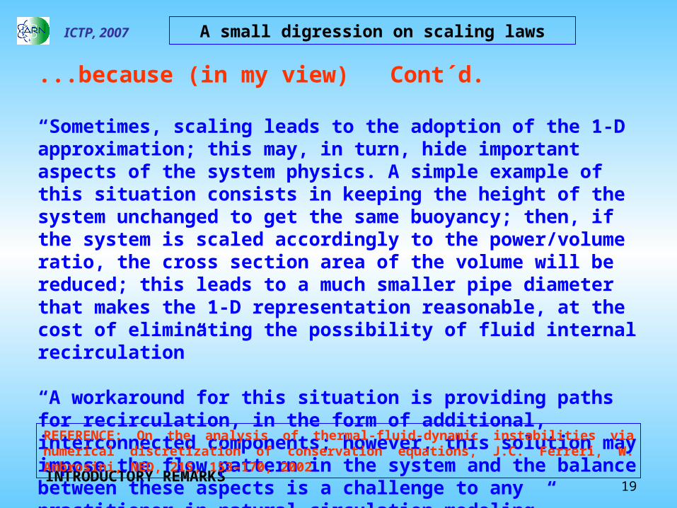
“Sometimes, scaling leads to the adoption of the 1-D approximation; this may, in turn, hide important aspects of the system physics. A simple example of this situation consists in keeping the height of the system unchanged to get the same buoyancy; then, if the system is scaled accordingly to the power/volume ratio, the cross section area of the volume will be reduced; this leads to a much smaller pipe diameter that makes the 1-D representation reasonable, at the cost of eliminating the possibility of fluid internal recirculation”
“A workaround for this situation is providing paths for recirculation, in the form of additional, interconnected components; however, this solution may impose the flow pattern in the system and the balance between these aspects is a challenge to any practitioner in natural circulation modeling”
REFERENCE: On the analysis of thermal-fluid-dynamic instabilities via numerical discretization of conservation equations, J.C. Ferreri, W. Ambrosini, NED, 215, 153–170, 2002
A small digression on scaling laws
20
ICTP, 2007
Then, in the following slides, some basic aspects of numerical techniques as applied to simple 1D problems
of physical significance will be reviewed
To start with, an exact, discrete approximation of a conservation like evolution equation will be developed
However (I believe)...
1D, thermal hydraulics system codes will be used at least for a decade or more, coupled with 3D modules for the core and/or for some specific components where separate effects
analysis is the goal.
INTRODUCTORY REMARKS
A small digression on scaling laws…
21
ICTP, 2007
INTRODUCTORY REMARKS
The balance equations
Two-Phase Fluid Models
Types of Constitutive Equations(Flow Regime Dependent)
Wall Friction (phase or mixture) correlationsWall Heat Transfer (phase or mixture) correlationsInterfacial Mass Transport EquationInterfacial Momentum Transport EquationInterfacial Energy Transport Equation
(2) Mass Conservation Equations(2) Momentum Conservation Equations(2) Energy Conservation Equations
Possible Restrictions
Equilibrium (Saturation)Partial Equilibrium
HomogeneousSlip ratioDrift flux
Velocity Temperature or Enthalpy
Two-Phase Fluid Model Calculated Parameters
6-Equation:
5-Equation:
4-Equation:
3-Equation:
vlvl TTvvp ,,,,,
mvl vTTp ,,,,
vlvl TorTvvp ,,,,
vl vvp ,,, lvm TorTvp ,,,
mvp,,
REFERENCE as provided: “Governing equations in two-phase fluid Natural circulation flows”, J.N. Reyes, jr, IAEA TECDOC 1474, 155-172, 2005
22
ICTP, 2007
ON NUMERICAL METHODS
Numerical approximations of conservation equations
Let us consider the following evolution equation, depending on time t and space x, where L is a linear operator.
Where HOT means terms of higher order. This equation may be formally written as:
K,1k,u)x
,x,t(Lt
uk
k
)x,t(u)Ltexp()x,t(u)t
texp()tt(u
u is the dependent variable. It may be expanded in Taylor series around t+t
Which is an explicit approximation to the evolution differential equation
HOTtt
u
!2
1t
t
u
!1
1x)u(t,x)t,u(t 2
2
2
23
ICTP, 2007
ON NUMERICAL METHODS
Numerical approximations of conservation equations
)x,t(u)L2
texp()tt(u)L
2
texp(
)x,t(u)tt(u)Ltexp(
)x,t(u)tt(u)3Ltexp()Ltexp()Ltexp( 21
By pre/post multiplying by suitable operators, implicit approximations may be obtained, like Crank Nicholson or fully implicit, as follows:
If L is a 3D operator, i.e. L = L1 + L2 + L3, the corresponding fully implicit approximation is:
24
ICTP, 2007
ON NUMERICAL METHODS
**3
***2
*1
u)tt(u)Ltexp(
uu)Ltexp(
)x,t(uu)Ltexp(
4
x
x
u
!2
1
2
x
x
u
!1
1u(x)x)
2
1u(x
2
2
2
Introducing intermediate definitions for u (they are not necessarily intermediate time approximations) then:
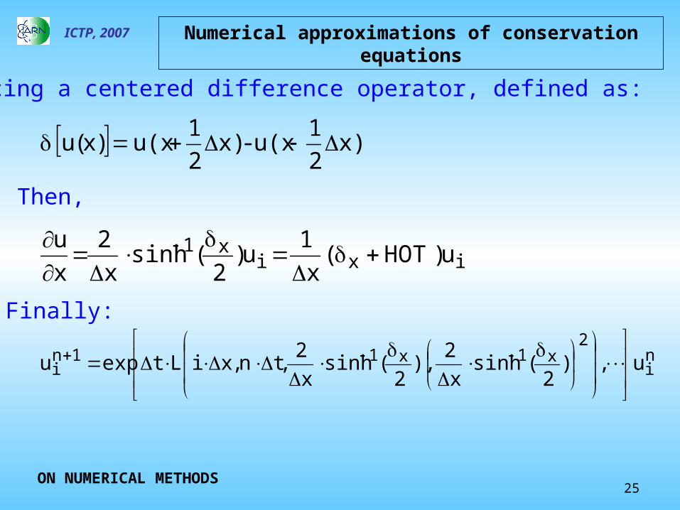
That is a sequence of 1D problems, known as an Aternating Direction Implicit method when L1, L2 and L3 depend on each space coordinate.Now, the discrete approximation in space will be introduced. It is:
Numerical approximations of conservation equations
25
ICTP, 2007
ON NUMERICAL METHODS
x)2
1u(x-x)
2
1u(x)x(u
ixix1 u)HOT(
x
1u)
2(sinh
x
2
x
u
ni
2x1x11n
i u,)2
(sinhx
2),
2(sinh
x
2,tn,xiLtexpu
Introducing a centered difference operator, defined as:
Then,
Finally:
Numerical approximations of conservation equations
26
ICTP, 2007
THE PREVIOUS EQUATION IS AN EXACT DISCRETE REPRESENTATION OF THE EVOLUTION EQUATION
In this form it is not useful for working
All practical approximation come from truncation of the seriesThis, in turn, implies the appearance of the truncation error of the approximation.
Postulate:TRUNCATION ERROR IS NOT A DISGRACE
Its adequate treatment allows the construction of useful working techniques.
ON NUMERICAL METHODS
Numerical approximations of conservation equations
27
ICTP, 2007
ON NUMERICAL METHODS
Three necessary definitions…
CONSISTENCYGiven a dependent variable that is sufficiently differentiable in a domain D and its boundary R, then, if an appropriate norm of the truncation errors L - Lh and B - Bh
tend to zero when the increments of the independent variables tend to zero in some way, then the discrete scheme Lh, Bh is said consistent with the differential
operators L, B
STABILITYGiven a function U defined in all the points of a grid in D and its boundary R,
then, if exists a finite quantity K such that in an appropriate norm, it is
})U(B)U(L{KU hh
for all the functions U defined in D+R, then the discrete scheme is said stable
Consistency and Stability may be conditional
28
ICTP, 2007
ON NUMERICAL METHODS
CONVERGENCEGiven a function U defined in all the points P of a grid in D and its boundary R, then, considering linear operators, if the discrete scheme is consistent and stable,
then the discrete scheme is convergent, i.e.:
zero totends)P(U)P(u
This is the equivalence theorem of P. Lax that allows constructing discrete, convergent solutions of a differential problem.
Three necessary definitions
29
ICTP, 2007
ON NUMERICAL METHODS
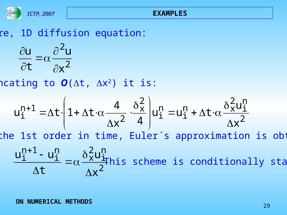
EXAMPLES
2
2
x
u
t
u
2
ni
2xn
ini
2x
21n
ix
utuu
4x
4t1tu
2
ni
2x
ni
1ni
x
u
t
uu
Pure, 1D diffusion equation:
Truncating to O(t, x2) it is:
Finally, the 1st order in time, Euler´s approximation is obtained:
This scheme is conditionally stable
30
ICTP, 2007
ON NUMERICAL METHODS
EXAMPLES
Linear, 1D scalar advection-diffusion equation
2
2
x
u
x
uC
t
u
0C;x
u
x2
uuC
t
uu2
ni
2x
n1i
n1i
ni
1ni
Approximating by centered differences, it is:
After expanding in Taylor series and keeping second order terms, it follows that:
Reference: Heuristic Stability Theory for FDE, C.W. Hirt, J. Comp. Phys., 2, pp. 339-355, 1968
)x,t(Ox
u
x
uC
t
u
2
t
t
u 222
2
2
2
31
ICTP, 2007 EXAMPLES
ON NUMERICAL METHODS
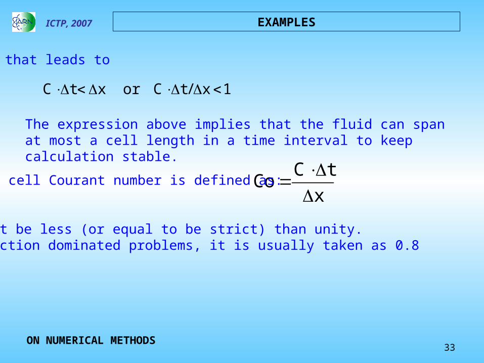
The previous expression clearly imposes: 02
tC2
)x,t(Ox
u)
2
tC(
x
uC
t
u 222
22
The previous expression is an hyperbolic differential equation and, in order that its domain of influence is to be contained in the domain of influence of the difference equation.
Coming back to the expanded difference equation and introducing the original differential equation, it follows that:
2
t
x
t
2
A necessary condition is that:
32
ICTP, 2007
ON NUMERICAL METHODS
0x
uC
t
u
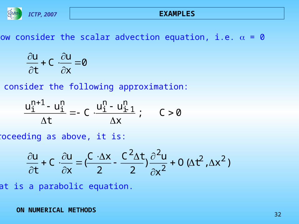
Let us now consider the scalar advection equation, i.e. = 0
and consider the following approximation:
0C;x
uuC
t
uu n1i
ni
ni
1ni
Proceeding as above, it is:
)x,t(Ox
u)
2
tC
2
xC(
x
uC
t
u 222
22
EXAMPLES
that is a parabolic equation.
33
ICTP, 2007
ON NUMERICAL METHODS
EXAMPLES
1x/tCor xtC
that leads to
The expression above implies that the fluid can span at most a cell length in a time interval to keep calculation stable.
x
tC Co
The cell Courant number is defined as:
and must be less (or equal to be strict) than unity. In advection dominated problems, it is usually taken as 0.8
34
ICTP, 2007
ON NUMERICAL METHODS
The non centered expression introduced is called an upwind approximation of the advection term and generates artificial or numerical diffusion that in the case of the transport of sharp waveforms or shock waves, smoothes the solution making it computable (the last concept was introduced by von Newman and Richtmyer in 1950)
In conjunction with the explicit time approximation constitutes the “Forward time, upwind space” approximation to the scalar wave equation or FTUS method.
This is the usual approximation used in the CFD codes to stabilize calculations or to regularize ill-posed models like in RELAP5, through the introduction of numerical diffusion. Many other methods have been developed with this philosophy. Adequate discretization permits keeping low truncation error and allowing the computation of unstable flows.
Reference: “A Method for the Numerical calculation of Hydrodynamic Shocks”, J. von Neumann and R.D. Richtmyer, J. Applied Phys., 31, pp. 232-237, 1950
EXAMPLES
35
ICTP, 2007
ON NUMERICAL METHODS
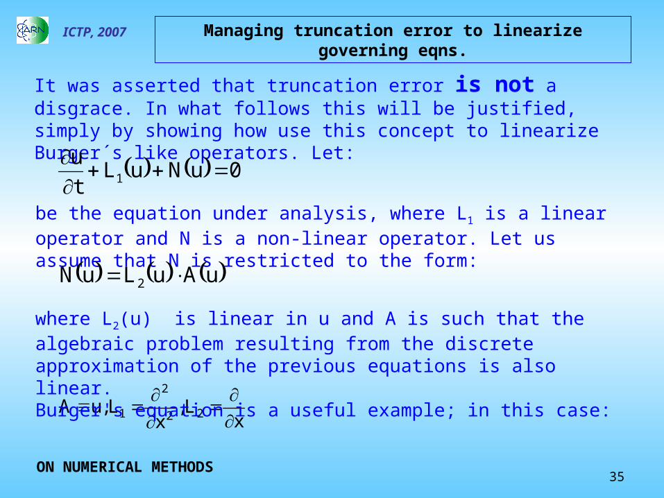
Managing truncation error to linearize governing eqns.
It was asserted that truncation error is not a disgrace. In what follows this will be justified, simply by showing how use this concept to linearize Burger´s like operators. Let:
be the equation under analysis, where L1 is a linear operator and N is a non-linear operator. Let us assume that N is restricted to the form:
0uNuLt
u1
uAuLuN 2
xL,
xL,uA 22
2
1
where L2(u) is linear in u and A is such that the algebraic problem resulting from the discrete approximation of the previous equations is also linear. Burger's equation is a useful example; in this case:
36
ICTP, 2007
A Crank-Nicholson approximation may be written as:
,tLA2
tL
2
tu
t
LA
t
L
2
ttLA
2
tL
2
tt
u
2
t
t
utu
32
*1
2*12
*1
2
22
O
where I is the identity operator and A* is a matrix independent of time and a suitable approximation to A to be defined in what follows.
nU1nU 2*
12*
1 LA2
tL
2
tILA
2
tL
2
tI
Expanding this expression in a Taylor series around n, we get:
Managing truncation error to linearize governing eqns.
ON NUMERICAL METHODS
37
ICTP, 2007
but, from the original equation:
t
LA
t
L
t
u 212
2
2222
*1 t
t
LA
2
t
t
L
2
tLAL
t
u O
Then, it follows that:
22*12
*12
2
tt
LA
t
L
2
tLAL
t
u
2
t
t
u O
Then,
Managing truncation error to linearize governing eqns.
ON NUMERICAL METHODS
38
ICTP, 2007
21
21
21 n
2nn
2* uLuAuLA
21n1
2 uL
21n* uAA
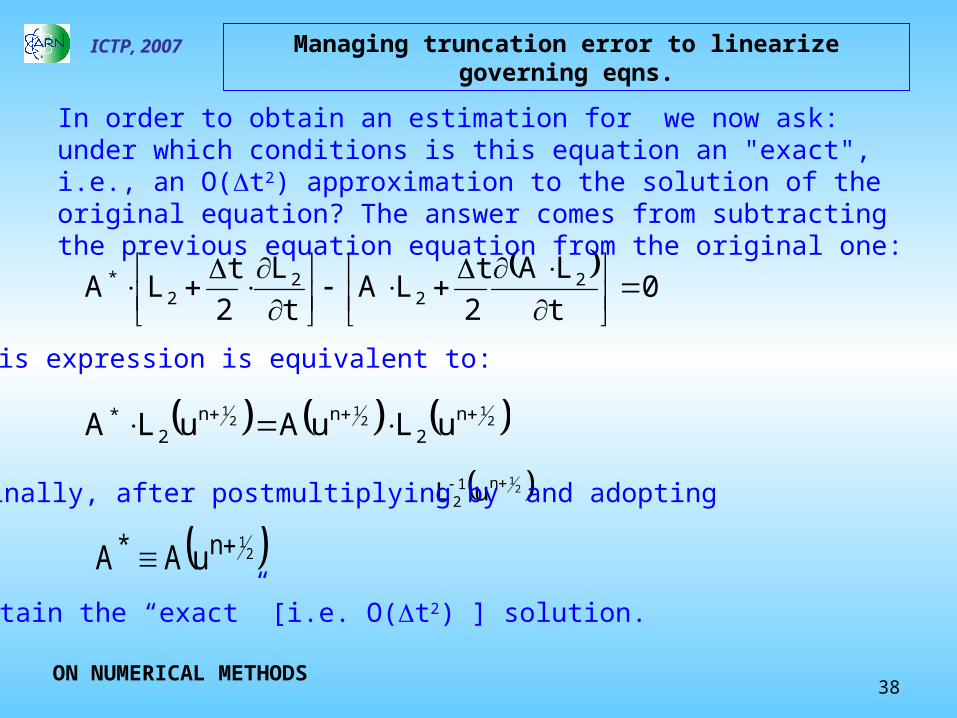
This expression is equivalent to:
Finally, after postmultiplying by and adopting
we obtain the “exact” [i.e. O(t2) ] solution.
Managing truncation error to linearize governing eqns.
ON NUMERICAL METHODS
0
t
LA
2
tLA
t
L
2
tLA 2
22
2*
In order to obtain an estimation for we now ask: under which conditions is this equation an "exact", i.e., an O(t2) approximation to the solution of the original equation? The answer comes from subtracting the previous equation equation from the original one:
39
ICTP, 2007
Because of the CN formulation, terms involving additional diffusion terms do not arise. If A* is evaluated as shown, then, the technique coincides with a predictor-corrector scheme based on the evaluation of "non-linear" coefficients evaluated at
This result is well known.
tntt 21
n
As may be observed from the above derivation, truncation error may be used, again, in a convenient way
Managing truncation error to linearize governing eqns.
ON NUMERICAL METHODS
40
ICTP, 2007
ON NUMERICAL METHODS
Dimensionless Time
Dim
ensi
onle
ss F
low
-10
-5
0
5
10
0 5 10 15
1000 Nodes
500 Modes +D(1000)
D(Q) =Q s
2
Q t
s
1
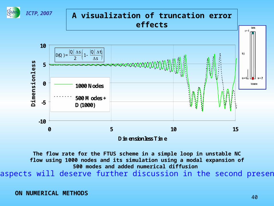
The flow rate for the FTUS scheme in a simple loop in unstable NC flow using 1000 nodes and its simulation using a modal expansion of 500 modes and added numerical diffusion
A visualization of truncation error effects
These aspects will deserve further discussion in the second presentation
41
ICTP, 2007
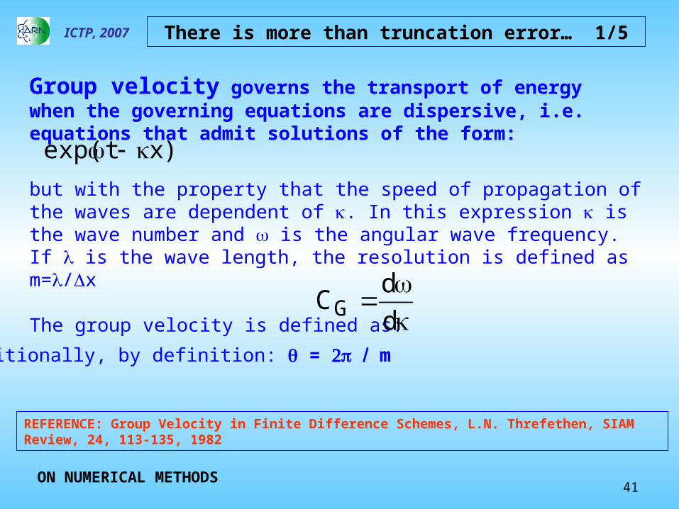
REFERENCE: Group Velocity in Finite Difference Schemes, L.N. Threfethen, SIAM Review, 24, 113-135, 1982
There is more than truncation error… 1/5
ON NUMERICAL METHODS
Group velocity governs the transport of energy when the governing equations are dispersive, i.e. equations that admit solutions of the form:
but with the property that the speed of propagation of the waves are dependent of . In this expression is the wave number and is the angular wave frequency. If is the wave length, the resolution is defined as m=/x
The group velocity is defined as:
)xtexp(
d
dCG
Additionally, by definition: = m
42
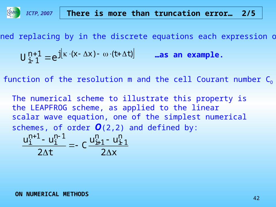
ICTP, 2007 There is more than truncation error… 2/5
ON NUMERICAL METHODS
It is obtained replacing by in the discrete equations each expression of U by:
)tt()xx(j1n1i eU …as an example.
and is a function of the resolution m and the cell Courant number CO
The numerical scheme to illustrate this property is the LEAPFROG scheme, as applied to the linear scalar wave equation, one of the simplest numerical
schemes, of order O(2,2) and defined by:
x2
uuC
t2
uu n1i
n1i
1ni
1ni
43
ICTP, 2007
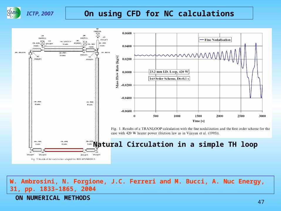
The illustration considers the LINEAR ADVECTION OF A SCALAR with two different wave forms, namely a smooth Gaussian and a wave packet.
In both cases, the transport velocity is C = 1, the space interval is Δx = 1/160, the Courant number is CO = 0.4, the resolution is m = 8 and the total time of integration is t = 2.
With the above parameters, the group velocity is 0.74
Why it is worth considering CFD approaches for CN, even in simple cases…
…through an example of how using well established, “natural” 1D laws in 1D TH loops to get non-conservative, wrong results
Let us consider the NC flow in a simple TH loop in unstable flow conditions
On using CFD for NC calculations
ON NUMERICAL METHODS
47
ICTP, 2007
W. Ambrosini, N. Forgione, J.C. Ferreri and M. Bucci, A. Nuc Energy, 31, pp. 1833–1865, 2004
Natural Circulation in a simple TH loop
On using CFD for NC calculations
ON NUMERICAL METHODS
48
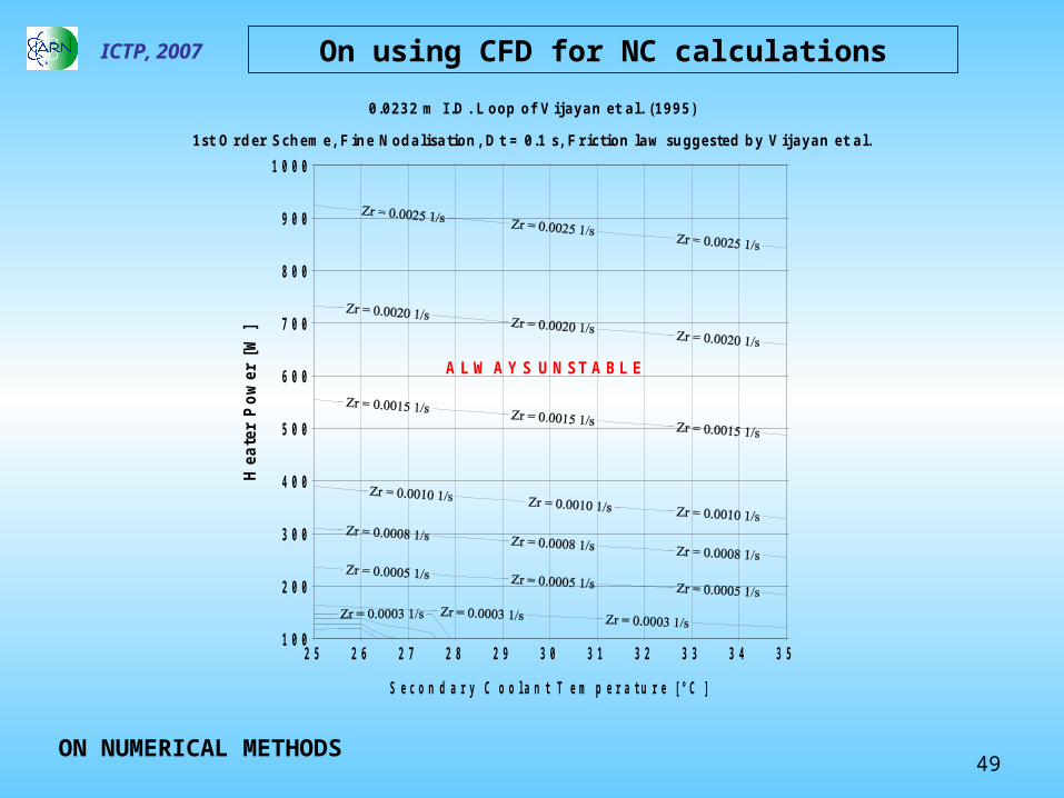
ICTP, 2007 On using CFD for NC calculations
ON NUMERICAL METHODS
49
ICTP, 2007 On using CFD for NC calculations
ON NUMERICAL METHODS
2 5 2 6 2 7 2 8 2 9 3 0 3 1 3 2 3 3 3 4 3 5
S e c o n d a r y C o o l a n t T e m p e r a t u r e [ ° C ]
1 0 0
2 0 0
3 0 0
4 0 0
5 0 0
6 0 0
7 0 0
8 0 0
9 0 0
1 0 0 0
Hea
ter
Pow
er [
W]
0 .0 2 3 2 m I .D . L o op o f V ija ya n e t a l. (1 9 9 5 )
1 st O rd er S ch em e, F in e N o d a lisa tio n , D t = 0 .1 s , F r ic tio n la w su gg ested b y V ija y an e t a l.
A L W A Y S U N S T A B L E
50
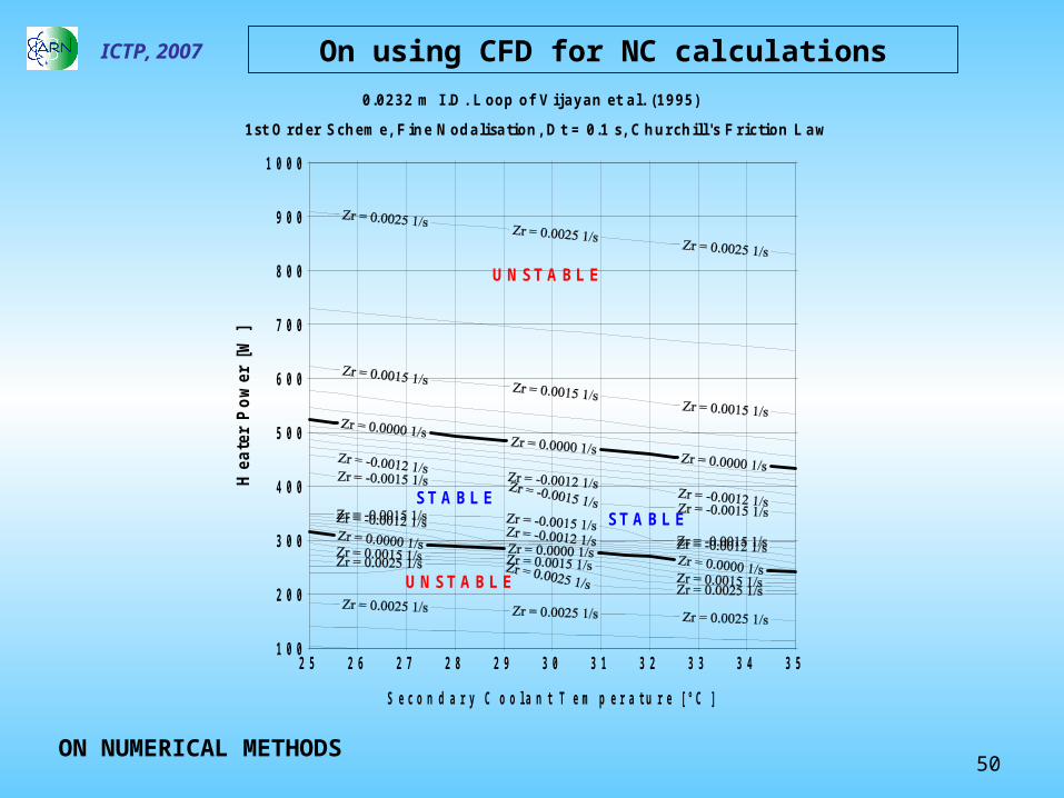
ICTP, 2007 On using CFD for NC calculations
ON NUMERICAL METHODS
2 5 2 6 2 7 2 8 2 9 3 0 3 1 3 2 3 3 3 4 3 5
S e c o n d a r y C o o l a n t T e m p e r a t u r e [ ° C ]
1 0 0
2 0 0
3 0 0
4 0 0
5 0 0
6 0 0
7 0 0
8 0 0
9 0 0
1 0 0 0
Hea
ter
Pow
er [
W]
0 .0 2 3 2 m I .D . L o op o f V ija ya n e t a l. (1 9 9 5 )
1 st O rd er S ch em e, F in e N o d a lisa tio n , D t = 0 .1 s , C h u rch ill's F r ic tio n L a w
U N S T A B L E
U N S T A B L E
S T A B L ES T A B L E
51
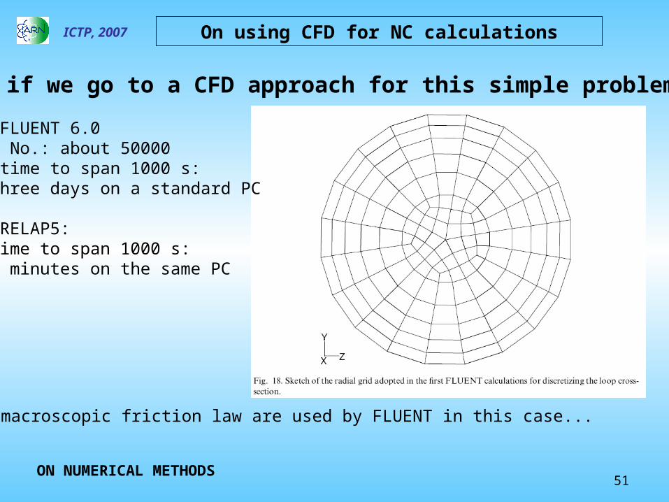
ICTP, 2007
What if we go to a CFD approach for this simple problem?
CODE: FLUENT 6.0 CELL No.: about 50000 CPU time to span 1000 s: three days on a standard PC
Using RELAP5: CPU time to span 1000 s: some minutes on the same PC
PS: no macroscopic friction law are used by FLUENT in this case...
On using CFD for NC calculations
ON NUMERICAL METHODS
52
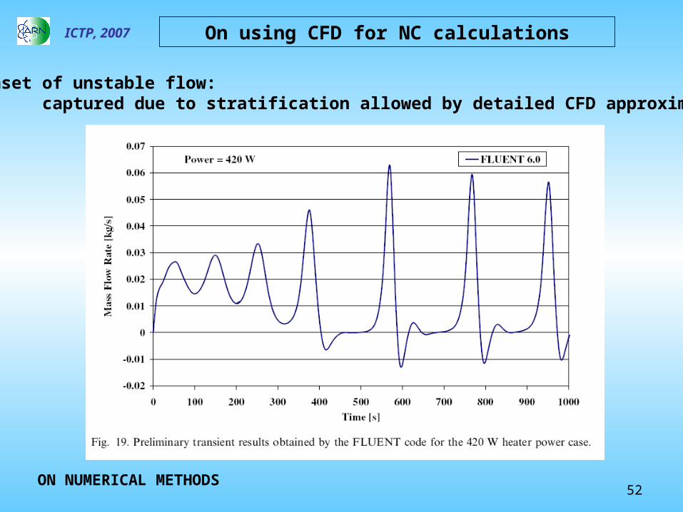
ICTP, 2007
Onset of unstable flow: captured due to stratification allowed by detailed CFD approximation
On using CFD for NC calculations
ON NUMERICAL METHODS
53
ICTP, 2007 On using CFD for NC calculations
ON NUMERICAL METHODS
54
ICTP, 2007
Evaluation of CFD methods for reactor safety analysis - ECORA - (12 partner institutions, see M. Scheuerer el al., NED, vol. 235, pp. 359-368, 2005)
• To show to end-users, utilities and regulators to which extent CFD can enhance the accuracy of safety analysis implies “addressing the lack of certainty on CFD results and defining related Best Practice Guidelines to evaluate these results”
Some collaborative efforts to elucidate the needs on CFD in relation to Nuclear Safety evaluations
On using CFD for NC calculations
ON THE PRESENT STATUS OF CFD IN RELATION TO NUCLEAR SAFETY
55
ICTP, 2007
From M. Scheuerer el al., NED, vol. 235, pp. 359-368, 2005
Objectives reached, according to authors:
• The establishment of BPGs for ensuring high-quality results and for the formalized judgment of CFD calculations and experimental data.
• The assessment of the potential, and of current limitations of CFD methods for flows in the primary system and in LWR containments, with special emphasis on PTS.
• The definition of experimental requirements for the verification and validation of CFD software for flows in the primary system and in LWR containments.
• The identification of improvements and extensions to the current CFD packages that are necessary for primary loop and containment flow analysis.
• The implementation and validation of improved turbulence and two-phase flow models for the simulation of PTS phenomena in PWR primary systems.
On using CFD for NC calculations
ON THE PRESENT STATUS OF CFD IN RELATION TO NUCLEAR SAFETY
56
ICTP, 2007
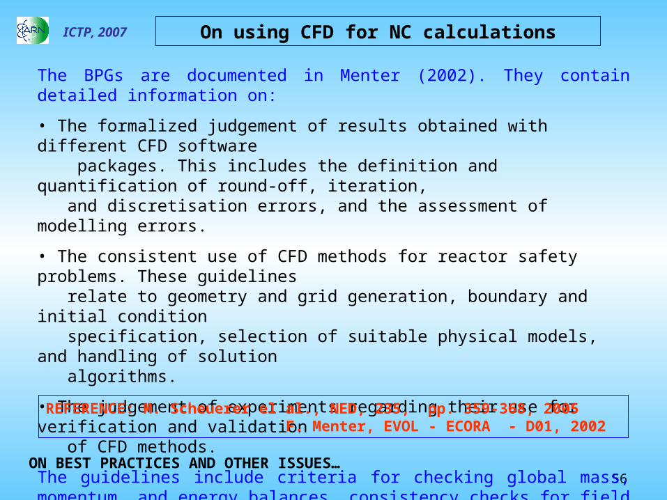
The BPGs are documented in Menter (2002). They contain detailed information on:
• The formalized judgement of results obtained with different CFD software packages. This includes the definition and quantification of round-off, iteration, and discretisation errors, and the assessment of modelling errors.
• The consistent use of CFD methods for reactor safety problems. These guidelines relate to geometry and grid generation, boundary and initial condition specification, selection of suitable physical models, and handling of solution algorithms.
• The judgement of experiments regarding their use for verification and validation of CFD methods.
The guidelines include criteria for checking global mass, momentum, and energy balances, consistency checks for field data, and plausibility checks. Experiments are grouped in a hierarchy ranging from laboratory studies to industrial field tests.The BPG report is intended as a living document.
REFERENCE: M. Scheuerer el al., NED, 235, pp. 359-368, 2005 F. Menter, EVOL - ECORA - D01, 2002
On using CFD for NC calculations
ON BEST PRACTICES AND OTHER ISSUES…
57
ICTP, 2007
Reference: A note on the Advection-Diffusion Equation, J.C. Ferreri, IJNMF, 5, pp.593-596, 1985
On wiggles and oscillations of the solutions
The 1-D advection-diffusion equation solution for different Peclet numbers. Points indicate the EXACT, STABLE solution using centered differences. The oscillating one is due to non appropriate boundary layer resolution. Asymptotic analysis or, more simply, introduction of upwinding eliminates the problem
ON BEST PRACTICES AND OTHER ISSUES…
58
ICTP, 2007 On wiggles and oscillations of the solutions
Reference: Heuristic Stability Theory for FDE, C.W. Hirt, J. Comp. Phys., 2, pp. 339-355, 1968
Non-linear coupling, Navier-Stokes eqns.NO UPWINDING - Halved time interval
ON BEST PRACTICES AND OTHER ISSUES…
59
ICTP, 2007
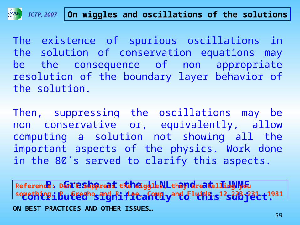
The existence of spurious oscillations in the solution of conservation equations may be the consequence of non appropriate resolution of the boundary layer behavior of the solution.
Then, suppressing the oscillations may be non conservative or, equivalently, allow computing a solution not showing all the important aspects of the physics. Work done in the 80´s served to clarify this aspects.
P. Gresho at the LLNL and at IJNMF contributed significantly to this subject.
On wiggles and oscillations of the solutions
Reference: Don´t suppress the wiggles, they are telling you something, P. Gresho and R. Lee, Comp. and Fluids, 12,223-231, 1981
ON BEST PRACTICES AND OTHER ISSUES…
60
ICTP, 2007
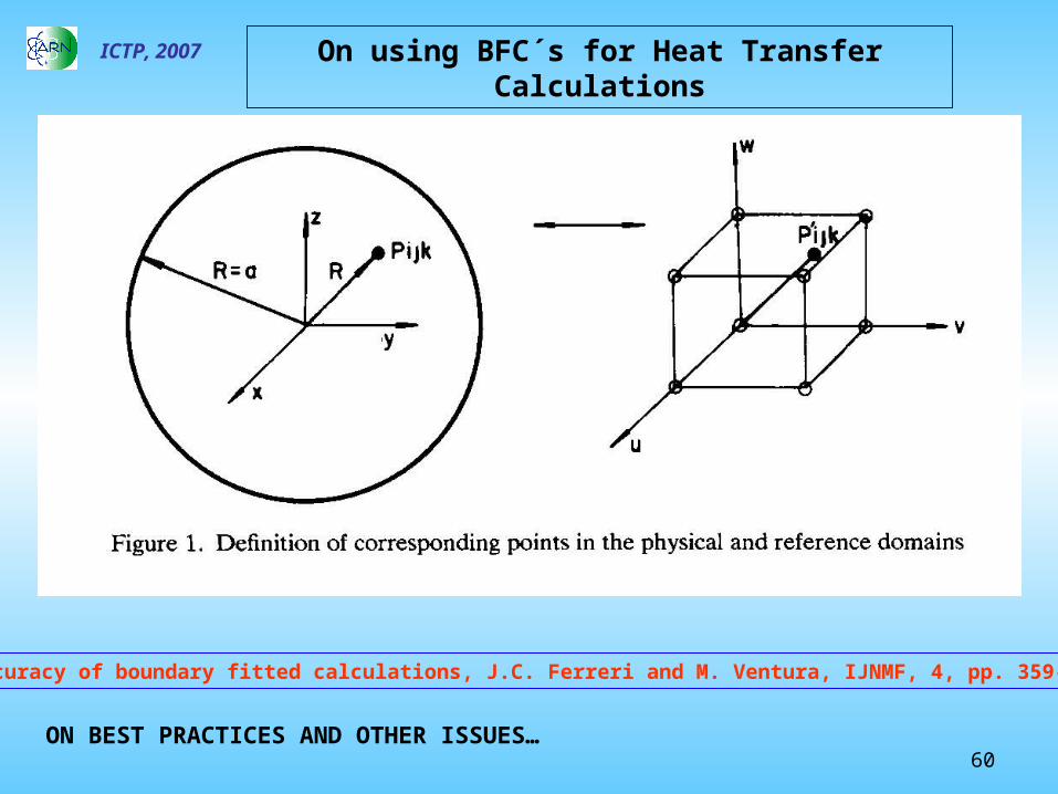
On the accuracy of boundary fitted calculations, J.C. Ferreri and M. Ventura, IJNMF, 4, pp. 359-375, 1984
ON BEST PRACTICES AND OTHER ISSUES…
On using BFC´s for Heat Transfer Calculations
61
ICTP, 2007
ON BEST PRACTICES AND OTHER ISSUES…
On using BFC´s for Heat Transfer Calculations
62
ICTP, 2007
ON BEST PRACTICES AND OTHER ISSUES…
On using BFC´s for Heat Transfer Calculations
It is simple to demonstrate that in the case of uniform heating, constant surface
temperature can only be obtained using regularly spaced grids at he surface and
nearby interior (see the effect of Biot number)
63
ICTP, 2007
ON BEST PRACTICES AND OTHER ISSUES…
On using BFC´s for Navier-Stokes Calculations
64
ICTP, 2007
ON BEST PRACTICES AND OTHER ISSUES…
On using BFC´s for Navier-Stokes Calculations
65
ICTP, 2007
The use of adaptive grids must be exercised with care. Even 1D cases may reflect the type of problems shown when the boundary conditions are of mixed (Robin) type.
The use of norms to get an insight of convergence of the solution should also be applied with care, because the solution may be almost perfect, but delayed or advanced in time depending on the scheme and its group velocity.
Oscillations in a computed solutions may be an indication of non appropriate discretization. Forcing its elimination may be a cause of losing information on the physics but, at the same time, making possible the calculation.
ON BEST PRACTICES AND OTHER ISSUES…
Some preliminary conclusions…
66
ICTP, 2007
Comments on BPGs
• BPGs are a valuable contribution to freshmen• Evaluation of results validity beyond the known experimental data base
range has always been one objective and an obvious difficulty of safety evaluations. Perhaps, whenever possible, designing SETs to interpolate should be a major goal to achieve
• I do not believe too much in written best practice guides. Perhaps emphasizing on the need of a discipline of analysis in depth and to promote pursuing well founded Engineering Judgement at the Academia should be enough. Anyway, BPGs may be a way to consolidate Engineering Judgement traditions…
PS: Ludwieg Prandtl (1875-1953) was surprised to learn that people used to teach with books written by other authors. Then…
ON BEST PRACTICES AND OTHER ISSUES…
On using CFD for NC calculations
67
ICTP, 2007
See also 1) Yadigaroglu et al., NED, vol. 221, pp. 205-223, 2003 on trends and needs in experimentation2) Rohde et al., NED, vol. 235, pp. 421-443, 2005 on fluid mixing in the reactor circuit
Advanced computational tools are needed for, at least:
• To implement further developments of existing physical models of two-phase flows, and the advanced, new ones proposed by the school of Ishii at Purdue and Lahey-Drew at RPI to deal with the smooth transitions in two-phase regimes, as opposed to fluid flow regime maps
• To develop and implement 3D, Two-Phase modules in commercial CFD software packages using friendly graphical user interfaces for the generation of grids and the visualization of results
• To develop multiple-field, multiple-scale, multi-dimensional analysis tools
• To verify and validate all the previously mentioned theories and implementations
On using CFD for NC calculations
ON THE PRESENT STATUS OF CFD IN RELATION TO NUCLEAR SAFETY
68
ICTP, 2007
See Guelfi et al., “A new multi-scale platform for advanced nuclear thermal-hydraulics status and prospects of the Neptune project”, NURETH 11, Avignon, France, 2005
• The NEPTUNE Project was launched at the end of 2001 by EDF and CEA.• The major underlying stakes for the nuclear industry partners are the
competitiveness of the reactors and the safety of Nuclear Power Plants.• The industrial situations which were identified as priority needs are all closely connected to these two major items• Examples:
1. The improved prediction of Departure from Nucleate Boiling(DNB) ranks among the high priority needs since it is directly linked to fuel performance.
2. The estimation of the fluid temperature field on the Reactor Pressure Vessel (RPV) in case of a Pressurized Thermal Shock (PTS) for controlling the lifespan of critical components.
3. The prediction of the maximum cladding temperature during a Large-Break LOCA
On using CFD for NC calculations
ON THE PRESENT STATUS OF CFD IN RELATION TO NUCLEAR SAFETY
69
ICTP, 2007
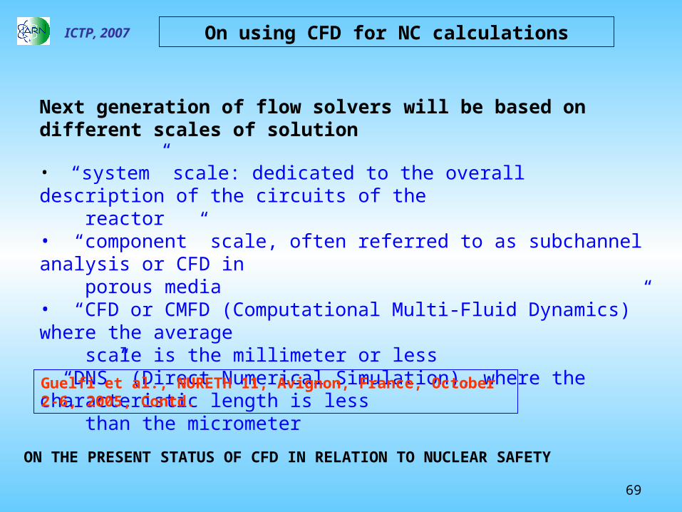
Next generation of flow solvers will be based on different scales of solution
• “system” scale: dedicated to the overall description of the circuits of the reactor• “component” scale, often referred to as subchannel analysis or CFD in porous media• “CFD or CMFD (Computational Multi-Fluid Dynamics)” where the average scale is the millimeter or less “DNS” (Direct Numerical Simulation), where the characteristic length is less than the micrometer
Guelfi et al., NURETH 11, Avignon, France, October 2-6, 2005, Contd.
On using CFD for NC calculations
ON THE PRESENT STATUS OF CFD IN RELATION TO NUCLEAR SAFETY
70
ICTP, 2007
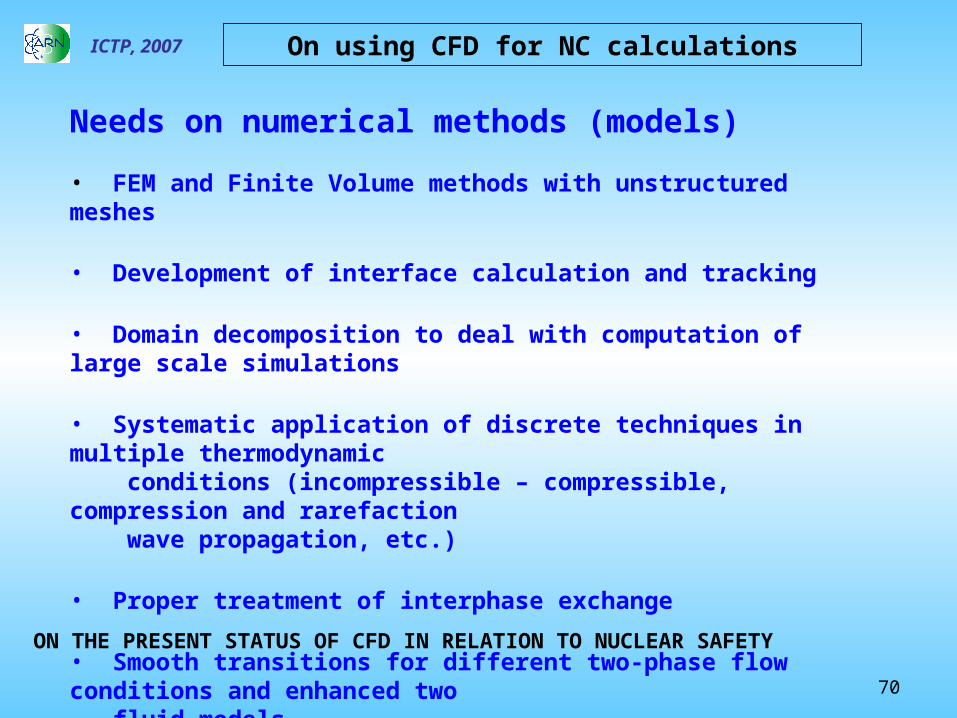
Needs on numerical methods (models)
• FEM and Finite Volume methods with unstructured meshes
• Development of interface calculation and tracking
• Domain decomposition to deal with computation of large scale simulations
• Systematic application of discrete techniques in multiple thermodynamic conditions (incompressible – compressible, compression and rarefaction wave propagation, etc.)
• Proper treatment of interphase exchange
• Smooth transitions for different two-phase flow conditions and enhanced two fluid models
On using CFD for NC calculations
ON THE PRESENT STATUS OF CFD IN RELATION TO NUCLEAR SAFETY
71
ICTP, 2007
On computers
• PCs clusters allow considering very detailed nodalizations (up to 300 106 FEM 3D elements grids are a –not too- common present practice with 200 PCs cluster) in the Computational Mechanics community. This allows computing the fluid flow distribution around a car in single-phase flow in a night
• For a NPP, in a two loop geometry, 100 m3 discretized at 1 cm3 scale implies considering 100 106 elements. Then, steady state in single phase seems reachable within today computing possibilities if a multiple-scale method is used… By the way, the flow distribution at a SG inlet has been reported recently using 1 106 elements and FLUENT RECALL that this implies having verified and validated parallelized algorithms as well as models amenable to this treatment
On using CFD for NC calculations
ON THE PRESENT STATUS OF CFD IN RELATION TO NUCLEAR SAFETY
72
ICTP, 2007
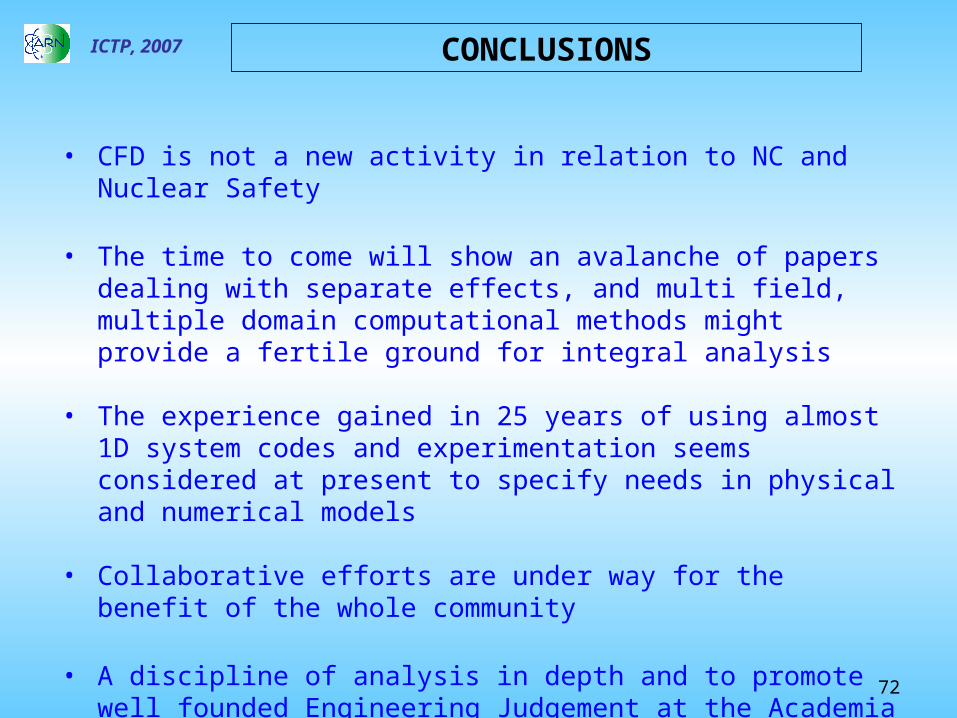
• CFD is not a new activity in relation to NC and Nuclear Safety
• The time to come will show an avalanche of papers dealing with separate effects, and multi field, multiple domain computational methods might provide a fertile ground for integral analysis
• The experience gained in 25 years of using almost 1D system codes and experimentation seems considered at present to specify needs in physical and numerical models
• Collaborative efforts are under way for the benefit of the whole community
• A discipline of analysis in depth and to promote well founded Engineering Judgement at the Academia would be worthwhile