Numerics Boundary Conditions Numerics and Boundary Conditions (used in PALM) PALM group Institute of Meteorology and Climatology, Leibniz Universit¨ at Hannover last update: 21st September 2015 PALM group PALM Seminar 1 / 22
Transcript
Numerics Boundary Conditions
Numerics and Boundary Conditions(used in PALM)
PALM group
Institute of Meteorology and Climatology, Leibniz Universitat Hannover
last update: 21st September 2015
PALM group PALM Seminar 1 / 22
Numerics Boundary Conditions
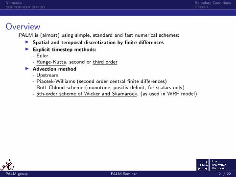
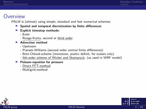
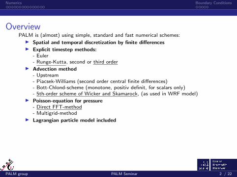
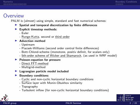
OverviewPALM is (almost) using simple, standard and fast numerical schemes:
I Spatial and temporal discretization by finite differencesI Explicit timestep methods:
- Euler- Runge-Kutta, second or third order
I Advection method- Upstream- Piacsek-Williams (second order central finite differences)- Bott-Chlond-scheme (monotone, positiv definit, for scalars only)- 5th-order scheme of Wicker and Skamarock, (as used in WRF model)
I Poisson-equation for pressure- Direct FFT-method- Multigrid-method
I Lagrangian particle model includedI Boundary conditions:
- Cyclic and non-cyclic horizontal boundary conditions- Surface layer with Monin-Obukhov similarity- Topography- Turbulent inflow (for non-cyclic horizontal boundary conditions)
PALM group PALM Seminar 2 / 22
Numerics Boundary Conditions
OverviewPALM is (almost) using simple, standard and fast numerical schemes:
I Spatial and temporal discretization by finite differences
I Explicit timestep methods:- Euler- Runge-Kutta, second or third order
I Advection method- Upstream- Piacsek-Williams (second order central finite differences)- Bott-Chlond-scheme (monotone, positiv definit, for scalars only)- 5th-order scheme of Wicker and Skamarock, (as used in WRF model)
I Poisson-equation for pressure- Direct FFT-method- Multigrid-method
I Lagrangian particle model includedI Boundary conditions:
- Cyclic and non-cyclic horizontal boundary conditions- Surface layer with Monin-Obukhov similarity- Topography- Turbulent inflow (for non-cyclic horizontal boundary conditions)
PALM group PALM Seminar 2 / 22
Numerics Boundary Conditions
OverviewPALM is (almost) using simple, standard and fast numerical schemes:
I Spatial and temporal discretization by finite differencesI Explicit timestep methods:
- Euler- Runge-Kutta, second or third order
I Advection method- Upstream- Piacsek-Williams (second order central finite differences)- Bott-Chlond-scheme (monotone, positiv definit, for scalars only)- 5th-order scheme of Wicker and Skamarock, (as used in WRF model)
I Poisson-equation for pressure- Direct FFT-method- Multigrid-method
I Lagrangian particle model includedI Boundary conditions:
- Cyclic and non-cyclic horizontal boundary conditions- Surface layer with Monin-Obukhov similarity- Topography- Turbulent inflow (for non-cyclic horizontal boundary conditions)
PALM group PALM Seminar 2 / 22
Numerics Boundary Conditions
OverviewPALM is (almost) using simple, standard and fast numerical schemes:
I Spatial and temporal discretization by finite differencesI Explicit timestep methods:
- Euler- Runge-Kutta, second or third order
I Advection method- Upstream- Piacsek-Williams (second order central finite differences)- Bott-Chlond-scheme (monotone, positiv definit, for scalars only)- 5th-order scheme of Wicker and Skamarock, (as used in WRF model)
I Poisson-equation for pressure- Direct FFT-method- Multigrid-method
I Lagrangian particle model included
I Boundary conditions:- Cyclic and non-cyclic horizontal boundary conditions- Surface layer with Monin-Obukhov similarity- Topography- Turbulent inflow (for non-cyclic horizontal boundary conditions)
PALM group PALM Seminar 2 / 22
Numerics Boundary Conditions
OverviewPALM is (almost) using simple, standard and fast numerical schemes:
I Spatial and temporal discretization by finite differencesI Explicit timestep methods:
- Euler- Runge-Kutta, second or third order
I Advection method- Upstream- Piacsek-Williams (second order central finite differences)- Bott-Chlond-scheme (monotone, positiv definit, for scalars only)- 5th-order scheme of Wicker and Skamarock, (as used in WRF model)
I Poisson-equation for pressure- Direct FFT-method- Multigrid-method
I Lagrangian particle model includedI Boundary conditions:
- Cyclic and non-cyclic horizontal boundary conditions- Surface layer with Monin-Obukhov similarity- Topography- Turbulent inflow (for non-cyclic horizontal boundary conditions)
PALM group PALM Seminar 2 / 22
Numerics Boundary Conditions
Numerics
Numerical Grid
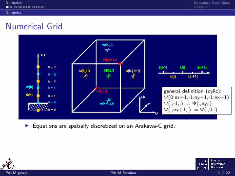
I Equations are spatially discretized on an Arakawa-C grid.
I All scalar variables s (e.g. , p∗, e, Km, Kh) are defined at the cell centers.
I Velocity components (u, v , w) are shifted by half of the grid spacing.
I Spacings are equidistant, stretching along z is possible.
general definition (cylic):Ψ(0:nz+1,-1:ny+1,-1:nx+1)Ψ(:,-1,:) = Ψ(:,ny,:)Ψ(:,ny+1,:) = Ψ(:,0,:)
PALM group PALM Seminar 3 / 22
Numerics Boundary Conditions
Numerics
Numerical Grid
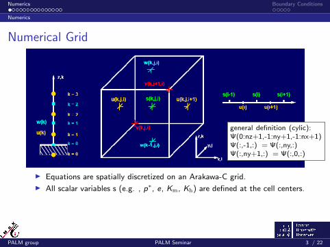
I Equations are spatially discretized on an Arakawa-C grid.
I All scalar variables s (e.g. , p∗, e, Km, Kh) are defined at the cell centers.
I Velocity components (u, v , w) are shifted by half of the grid spacing.
I Spacings are equidistant, stretching along z is possible.
general definition (cylic):Ψ(0:nz+1,-1:ny+1,-1:nx+1)Ψ(:,-1,:) = Ψ(:,ny,:)Ψ(:,ny+1,:) = Ψ(:,0,:)
PALM group PALM Seminar 3 / 22
Numerics Boundary Conditions
Numerics
Numerical Grid
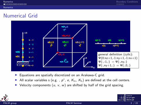
I Equations are spatially discretized on an Arakawa-C grid.
I All scalar variables s (e.g. , p∗, e, Km, Kh) are defined at the cell centers.
I Velocity components (u, v , w) are shifted by half of the grid spacing.
I Spacings are equidistant, stretching along z is possible.
general definition (cylic):Ψ(0:nz+1,-1:ny+1,-1:nx+1)Ψ(:,-1,:) = Ψ(:,ny,:)Ψ(:,ny+1,:) = Ψ(:,0,:)
PALM group PALM Seminar 3 / 22
Numerics Boundary Conditions
Numerics
Numerical Grid
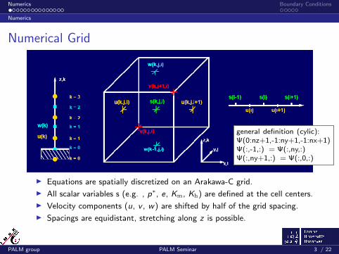
I Equations are spatially discretized on an Arakawa-C grid.
I All scalar variables s (e.g. , p∗, e, Km, Kh) are defined at the cell centers.
I Velocity components (u, v , w) are shifted by half of the grid spacing.
I Spacings are equidistant, stretching along z is possible.
general definition (cylic):Ψ(0:nz+1,-1:ny+1,-1:nx+1)Ψ(:,-1,:) = Ψ(:,ny,:)Ψ(:,ny+1,:) = Ψ(:,0,:)
PALM group PALM Seminar 3 / 22
Numerics Boundary Conditions
Numerics
Timestep Methods (I)
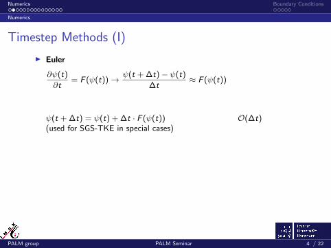
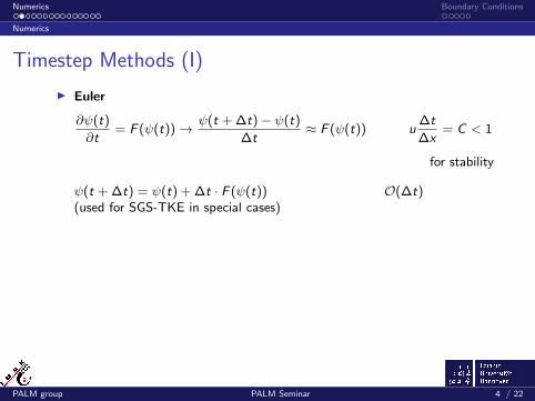
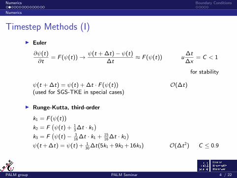
I Euler
∂ψ(t)
∂t= F (ψ(t))→ ψ(t + ∆t)− ψ(t)
∆t≈ F (ψ(t))
u∆t
∆x= C < 1
for stability
ψ(t + ∆t) = ψ(t) + ∆t · F (ψ(t)) O(∆t)(used for SGS-TKE in special cases)
I Runge-Kutta, third-order
k1 = F (ψ(t))
k2 = F(ψ(t) + 1
3∆t · k1
)k3 = F
(ψ(t)− 3
16∆t · k1 + 15
16∆t · k2
)ψ(t + ∆t) = ψ(t) + 1
30∆t(5k1 + 9k2 + 16k3) O(∆t2) C ≤ 0.9
PALM group PALM Seminar 4 / 22
Numerics Boundary Conditions
Numerics
Timestep Methods (I)
I Euler
∂ψ(t)
∂t= F (ψ(t))→ ψ(t + ∆t)− ψ(t)
∆t≈ F (ψ(t)) u
∆t
∆x= C < 1
for stability
ψ(t + ∆t) = ψ(t) + ∆t · F (ψ(t)) O(∆t)(used for SGS-TKE in special cases)
I Runge-Kutta, third-order
k1 = F (ψ(t))
k2 = F(ψ(t) + 1
3∆t · k1
)k3 = F
(ψ(t)− 3
16∆t · k1 + 15
16∆t · k2
)ψ(t + ∆t) = ψ(t) + 1
30∆t(5k1 + 9k2 + 16k3) O(∆t2) C ≤ 0.9
PALM group PALM Seminar 4 / 22
Numerics Boundary Conditions
Numerics
Timestep Methods (II)
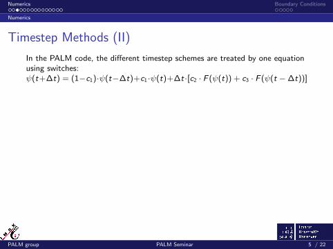
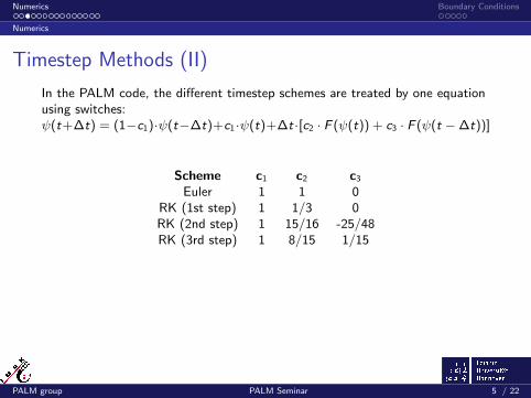
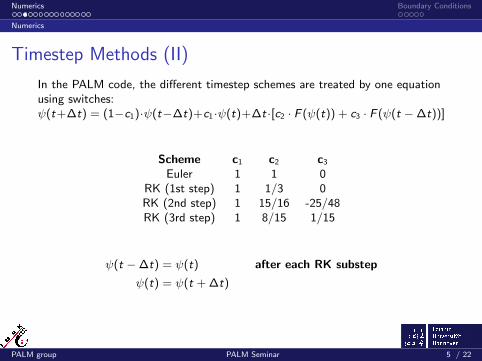
In the PALM code, the different timestep schemes are treated by one equationusing switches:ψ(t+∆t) = (1−c1)·ψ(t−∆t)+c1 ·ψ(t)+∆t ·[c2 · F (ψ(t)) + c3 · F (ψ(t −∆t))]
In the PALM code, the different timestep schemes are treated by one equationusing switches:ψ(t+∆t) = (1−c1)·ψ(t−∆t)+c1 ·ψ(t)+∆t ·[c2 · F (ψ(t)) + c3 · F (ψ(t −∆t))]
In the PALM code, the different timestep schemes are treated by one equationusing switches:ψ(t+∆t) = (1−c1)·ψ(t−∆t)+c1 ·ψ(t)+∆t ·[c2 · F (ψ(t)) + c3 · F (ψ(t −∆t))]
I Piacsek Williams C3 (1970, J. Comput. Phy., 6, 392).
I Scheme of 2nd order accuracy.
I Conserves integrals of linear and quadratic quantities.
I Requires incompressibility → flux form of advection term.
∂(uψ)
∂x
∣∣∣∣i
=1
2∆x
(ui+ 1
2ψi+1 − ui− 1
2ψi−1
)
I In case of momentum advection (e.g. ψ = u), ui−1 and ui+1 haveto be obtained by linear interpolation.
I May cause 2∆x wiggles in case of sharp gradients.
PALM group PALM Seminar 6 / 22
Numerics Boundary Conditions
Numerics
Advection Methods (I)
I Piacsek Williams C3 (1970, J. Comput. Phy., 6, 392).
I Scheme of 2nd order accuracy.
I Conserves integrals of linear and quadratic quantities.
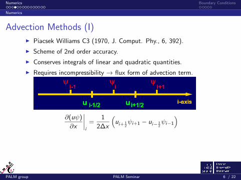
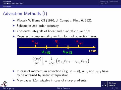
I Requires incompressibility → flux form of advection term.
∂(uψ)
∂x
∣∣∣∣i
=1
2∆x
(ui+ 1
2ψi+1 − ui− 1
2ψi−1
)I In case of momentum advection (e.g. ψ = u), ui−1 and ui+1 have
to be obtained by linear interpolation.
I May cause 2∆x wiggles in case of sharp gradients.
PALM group PALM Seminar 6 / 22
Numerics Boundary Conditions
Numerics
Advection Methods (II)
I Bott-Chlond- Chlond (1994)
- Monotone, positive definit. Can only be used for scalars- Conserves sharp gradients- Numerically expensive- Not optimized for use on cache-based machines.
I Default: Wicker and Skamarock scheme (5th order)- Much better accuracy than Piacsek Williams- Much simpler algorithm than Bott-Chlond- Requires additional ghost layers- Adds additional numerical dissipation
PALM group PALM Seminar 7 / 22
Numerics Boundary Conditions
Numerics
Advection Methods (II)
I Bott-Chlond- Chlond (1994)- Monotone, positive definit. Can only be used for scalars
- Conserves sharp gradients- Numerically expensive- Not optimized for use on cache-based machines.
I Default: Wicker and Skamarock scheme (5th order)- Much better accuracy than Piacsek Williams- Much simpler algorithm than Bott-Chlond- Requires additional ghost layers- Adds additional numerical dissipation
PALM group PALM Seminar 7 / 22
Numerics Boundary Conditions
Numerics
Advection Methods (II)
I Bott-Chlond- Chlond (1994)- Monotone, positive definit. Can only be used for scalars- Conserves sharp gradients
- Numerically expensive- Not optimized for use on cache-based machines.
I Default: Wicker and Skamarock scheme (5th order)- Much better accuracy than Piacsek Williams- Much simpler algorithm than Bott-Chlond- Requires additional ghost layers- Adds additional numerical dissipation
PALM group PALM Seminar 7 / 22
Numerics Boundary Conditions
Numerics
Advection Methods (II)
I Bott-Chlond- Chlond (1994)- Monotone, positive definit. Can only be used for scalars- Conserves sharp gradients- Numerically expensive
- Not optimized for use on cache-based machines.
I Default: Wicker and Skamarock scheme (5th order)- Much better accuracy than Piacsek Williams- Much simpler algorithm than Bott-Chlond- Requires additional ghost layers- Adds additional numerical dissipation
PALM group PALM Seminar 7 / 22
Numerics Boundary Conditions
Numerics
Advection Methods (II)
I Bott-Chlond- Chlond (1994)- Monotone, positive definit. Can only be used for scalars- Conserves sharp gradients- Numerically expensive- Not optimized for use on cache-based machines.
I Default: Wicker and Skamarock scheme (5th order)
- Much better accuracy than Piacsek Williams- Much simpler algorithm than Bott-Chlond- Requires additional ghost layers- Adds additional numerical dissipation
PALM group PALM Seminar 7 / 22
Numerics Boundary Conditions
Numerics
Advection Methods (II)
I Bott-Chlond- Chlond (1994)- Monotone, positive definit. Can only be used for scalars- Conserves sharp gradients- Numerically expensive- Not optimized for use on cache-based machines.
I Default: Wicker and Skamarock scheme (5th order)- Much better accuracy than Piacsek Williams
- Much simpler algorithm than Bott-Chlond- Requires additional ghost layers- Adds additional numerical dissipation
PALM group PALM Seminar 7 / 22
Numerics Boundary Conditions
Numerics
Advection Methods (II)
I Bott-Chlond- Chlond (1994)- Monotone, positive definit. Can only be used for scalars- Conserves sharp gradients- Numerically expensive- Not optimized for use on cache-based machines.
I Default: Wicker and Skamarock scheme (5th order)- Much better accuracy than Piacsek Williams- Much simpler algorithm than Bott-Chlond
I Bott-Chlond- Chlond (1994)- Monotone, positive definit. Can only be used for scalars- Conserves sharp gradients- Numerically expensive- Not optimized for use on cache-based machines.
I Default: Wicker and Skamarock scheme (5th order)- Much better accuracy than Piacsek Williams- Much simpler algorithm than Bott-Chlond- Requires additional ghost layers
- Adds additional numerical dissipation
PALM group PALM Seminar 7 / 22
Numerics Boundary Conditions
Numerics
Advection Methods (II)
I Bott-Chlond- Chlond (1994)- Monotone, positive definit. Can only be used for scalars- Conserves sharp gradients- Numerically expensive- Not optimized for use on cache-based machines.
I Default: Wicker and Skamarock scheme (5th order)- Much better accuracy than Piacsek Williams- Much simpler algorithm than Bott-Chlond- Requires additional ghost layers- Adds additional numerical dissipation
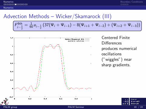
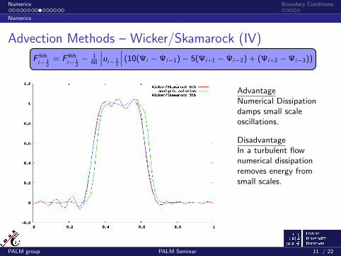
AdvantageNumerical Dissipationdamps small scaleoscillations.
DisadvantageIn a turbulent flownumerical dissipationremoves energy fromsmall scales.
PALM group PALM Seminar 11 / 22
Numerics Boundary Conditions
Numerics
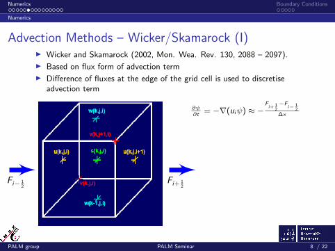
Advection Methods – Wicker/Skamarock (V)
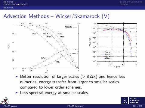
I Better resolution of larger scales (> 8 ∆x) and hence lessnumerical energy transfer from larger to smaller scalescompared to lower order schemes.
I Less spectral energy at smaller scales.
PALM group PALM Seminar 12 / 22
Numerics Boundary Conditions
Numerics
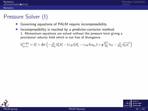
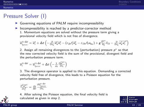
Pressure Solver (I)I Governing equations of PALM require incompressibility
I Incompressibility is reached by a predictor-corrector method1. Momentum equations are solved without the pressure term giving aprovisional velocity field which is not free of divergence.
ut+∆tiprov
= uti + ∆t(− ∂∂xk
utkuti − (εijk fju
tk − εi3k f3ugk ) + g θ
∗t
θ0δi3 − ∂
∂xku′ku′i
t)
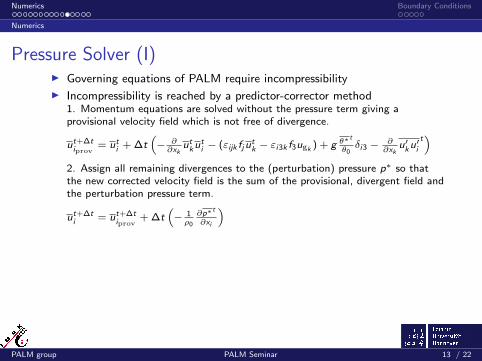
2. Assign all remaining divergences to the (perturbation) pressure p∗ so thatthe new corrected velocity field is the sum of the provisional, divergent field andthe perturbation pressure term.
ut+∆ti = ut+∆t
iprov+ ∆t
(− 1ρ0
∂p∗t
∂xi
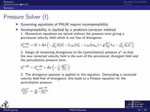
)3. The divergence operator is applied to this equation. Demanding a correctedvelocity field free of divergence, this leads to a Poisson equation for theperturbation pressure.
∂2p∗t
∂x2i
= ρ0∆t
∂ut+∆tiprov
∂xi
4. After solving the Poisson equation, the final velocity field iscalculated as given in step 2.
PALM group PALM Seminar 13 / 22
Numerics Boundary Conditions
Numerics
Pressure Solver (I)I Governing equations of PALM require incompressibility
I Incompressibility is reached by a predictor-corrector method1. Momentum equations are solved without the pressure term giving aprovisional velocity field which is not free of divergence.
ut+∆tiprov
= uti + ∆t(− ∂∂xk
utkuti − (εijk fju
tk − εi3k f3ugk ) + g θ
∗t
θ0δi3 − ∂
∂xku′ku′i
t)
2. Assign all remaining divergences to the (perturbation) pressure p∗ so thatthe new corrected velocity field is the sum of the provisional, divergent field andthe perturbation pressure term.
ut+∆ti = ut+∆t
iprov+ ∆t
(− 1ρ0
∂p∗t
∂xi
)
3. The divergence operator is applied to this equation. Demanding a correctedvelocity field free of divergence, this leads to a Poisson equation for theperturbation pressure.
∂2p∗t
∂x2i
= ρ0∆t
∂ut+∆tiprov
∂xi
4. After solving the Poisson equation, the final velocity field iscalculated as given in step 2.
PALM group PALM Seminar 13 / 22
Numerics Boundary Conditions
Numerics
Pressure Solver (I)I Governing equations of PALM require incompressibility
I Incompressibility is reached by a predictor-corrector method1. Momentum equations are solved without the pressure term giving aprovisional velocity field which is not free of divergence.
ut+∆tiprov
= uti + ∆t(− ∂∂xk
utkuti − (εijk fju
tk − εi3k f3ugk ) + g θ
∗t
θ0δi3 − ∂
∂xku′ku′i
t)
2. Assign all remaining divergences to the (perturbation) pressure p∗ so thatthe new corrected velocity field is the sum of the provisional, divergent field andthe perturbation pressure term.
ut+∆ti = ut+∆t
iprov+ ∆t
(− 1ρ0
∂p∗t
∂xi
)3. The divergence operator is applied to this equation. Demanding a correctedvelocity field free of divergence, this leads to a Poisson equation for theperturbation pressure.
∂2p∗t
∂x2i
= ρ0∆t
∂ut+∆tiprov
∂xi
4. After solving the Poisson equation, the final velocity field iscalculated as given in step 2.
PALM group PALM Seminar 13 / 22
Numerics Boundary Conditions
Numerics
Pressure Solver (I)I Governing equations of PALM require incompressibility
I Incompressibility is reached by a predictor-corrector method1. Momentum equations are solved without the pressure term giving aprovisional velocity field which is not free of divergence.
ut+∆tiprov
= uti + ∆t(− ∂∂xk
utkuti − (εijk fju
tk − εi3k f3ugk ) + g θ
∗t
θ0δi3 − ∂
∂xku′ku′i
t)
2. Assign all remaining divergences to the (perturbation) pressure p∗ so thatthe new corrected velocity field is the sum of the provisional, divergent field andthe perturbation pressure term.
ut+∆ti = ut+∆t
iprov+ ∆t
(− 1ρ0
∂p∗t
∂xi
)3. The divergence operator is applied to this equation. Demanding a correctedvelocity field free of divergence, this leads to a Poisson equation for theperturbation pressure.
∂2p∗t
∂x2i
= ρ0∆t
∂ut+∆tiprov
∂xi
4. After solving the Poisson equation, the final velocity field iscalculated as given in step 2.
PALM group PALM Seminar 13 / 22
Numerics Boundary Conditions
Numerics
Pressure Solver (II)
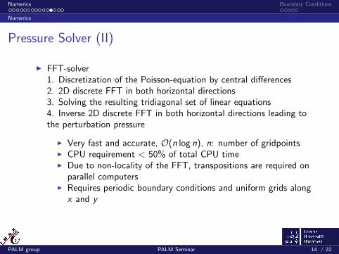
I FFT-solver1. Discretization of the Poisson-equation by central differences
2. 2D discrete FFT in both horizontal directions3. Solving the resulting tridiagonal set of linear equations4. Inverse 2D discrete FFT in both horizontal directions leading tothe perturbation pressure
I Very fast and accurate, O(n log n), n: number of gridpointsI CPU requirement < 50% of total CPU timeI Due to non-locality of the FFT, transpositions are required on
parallel computersI Requires periodic boundary conditions and uniform grids along
x and y
PALM group PALM Seminar 14 / 22
Numerics Boundary Conditions
Numerics
Pressure Solver (II)
I FFT-solver1. Discretization of the Poisson-equation by central differences2. 2D discrete FFT in both horizontal directions
3. Solving the resulting tridiagonal set of linear equations4. Inverse 2D discrete FFT in both horizontal directions leading tothe perturbation pressure
I Very fast and accurate, O(n log n), n: number of gridpointsI CPU requirement < 50% of total CPU timeI Due to non-locality of the FFT, transpositions are required on
parallel computersI Requires periodic boundary conditions and uniform grids along
x and y
PALM group PALM Seminar 14 / 22
Numerics Boundary Conditions
Numerics
Pressure Solver (II)
I FFT-solver1. Discretization of the Poisson-equation by central differences2. 2D discrete FFT in both horizontal directions3. Solving the resulting tridiagonal set of linear equations
4. Inverse 2D discrete FFT in both horizontal directions leading tothe perturbation pressure
I Very fast and accurate, O(n log n), n: number of gridpointsI CPU requirement < 50% of total CPU timeI Due to non-locality of the FFT, transpositions are required on
parallel computersI Requires periodic boundary conditions and uniform grids along
x and y
PALM group PALM Seminar 14 / 22
Numerics Boundary Conditions
Numerics
Pressure Solver (II)
I FFT-solver1. Discretization of the Poisson-equation by central differences2. 2D discrete FFT in both horizontal directions3. Solving the resulting tridiagonal set of linear equations4. Inverse 2D discrete FFT in both horizontal directions leading tothe perturbation pressure
I Very fast and accurate, O(n log n), n: number of gridpoints
I CPU requirement < 50% of total CPU timeI Due to non-locality of the FFT, transpositions are required on
parallel computersI Requires periodic boundary conditions and uniform grids along
x and y
PALM group PALM Seminar 14 / 22
Numerics Boundary Conditions
Numerics
Pressure Solver (II)
I FFT-solver1. Discretization of the Poisson-equation by central differences2. 2D discrete FFT in both horizontal directions3. Solving the resulting tridiagonal set of linear equations4. Inverse 2D discrete FFT in both horizontal directions leading tothe perturbation pressure
I Very fast and accurate, O(n log n), n: number of gridpointsI CPU requirement < 50% of total CPU time
I Due to non-locality of the FFT, transpositions are required onparallel computers
I Requires periodic boundary conditions and uniform grids alongx and y
PALM group PALM Seminar 14 / 22
Numerics Boundary Conditions
Numerics
Pressure Solver (II)
I FFT-solver1. Discretization of the Poisson-equation by central differences2. 2D discrete FFT in both horizontal directions3. Solving the resulting tridiagonal set of linear equations4. Inverse 2D discrete FFT in both horizontal directions leading tothe perturbation pressure
I Very fast and accurate, O(n log n), n: number of gridpointsI CPU requirement < 50% of total CPU timeI Due to non-locality of the FFT, transpositions are required on
parallel computers
I Requires periodic boundary conditions and uniform grids alongx and y
PALM group PALM Seminar 14 / 22
Numerics Boundary Conditions
Numerics
Pressure Solver (II)
I FFT-solver1. Discretization of the Poisson-equation by central differences2. 2D discrete FFT in both horizontal directions3. Solving the resulting tridiagonal set of linear equations4. Inverse 2D discrete FFT in both horizontal directions leading tothe perturbation pressure
I Very fast and accurate, O(n log n), n: number of gridpointsI CPU requirement < 50% of total CPU timeI Due to non-locality of the FFT, transpositions are required on
parallel computersI Requires periodic boundary conditions and uniform grids along
x and y
PALM group PALM Seminar 14 / 22
Numerics Boundary Conditions
Numerics
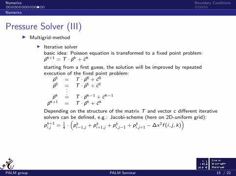
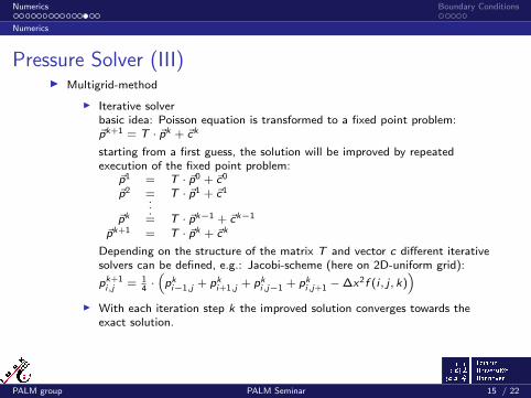
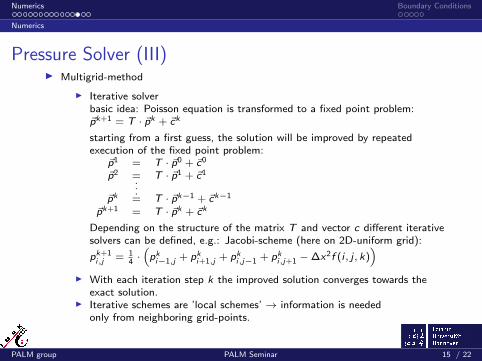
Pressure Solver (III)I Multigrid-method
I Iterative solverbasic idea: Poisson equation is transformed to a fixed point problem:~pk+1 = T · ~pk + ~ck
starting from a first guess, the solution will be improved by repeatedexecution of the fixed point problem:
~p1 = T · ~p0 + ~c0
~p2 = T · ~p1 + ~c1...
~pk = T · ~pk−1 + ~ck−1
~pk+1 = T · ~pk + ~ck
Depending on the structure of the matrix T and vector c different iterativesolvers can be defined, e.g.: Jacobi-scheme (here on 2D-uniform grid):
)I With each iteration step k the improved solution converges towards the
exact solution.I Iterative schemes are ’local schemes’ → information is needed
only from neighboring grid-points.I Very low convergence: O(n2).
PALM group PALM Seminar 15 / 22
Numerics Boundary Conditions
Numerics
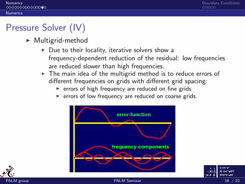
Pressure Solver (IV)I Multigrid-method
I Due to their locality, iterative solvers show afrequency-dependent reduction of the residual: low frequenciesare reduced slower than high frequencies.
I The main idea of the multigrid method is to reduce errors ofdifferent frequencies on grids with different grid spacing:
I errors of high frequency are reduced on fine gridsI errors of low frequency are reduced on coarse grids.
PALM group PALM Seminar 16 / 22
Numerics Boundary Conditions
Numerics
Pressure Solver (V)
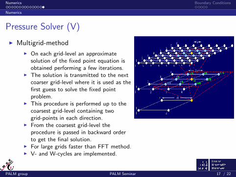
I Multigrid-method
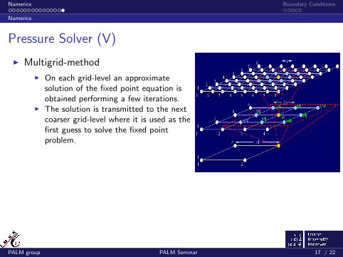
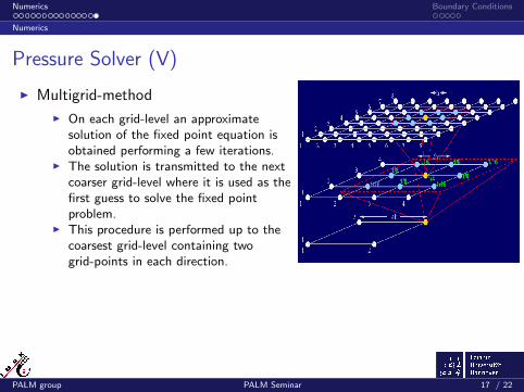
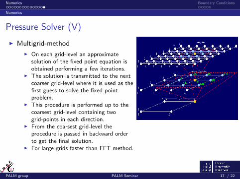
I On each grid-level an approximatesolution of the fixed point equation isobtained performing a few iterations.
I The solution is transmitted to the nextcoarser grid-level where it is used as thefirst guess to solve the fixed pointproblem.
I This procedure is performed up to thecoarsest grid-level containing twogrid-points in each direction.
I From the coarsest grid-level theprocedure is passed in backward orderto get the final solution.
I For large grids faster than FFT method.I V- and W-cycles are implemented.
PALM group PALM Seminar 17 / 22
Numerics Boundary Conditions
Numerics
Pressure Solver (V)
I Multigrid-method
I On each grid-level an approximatesolution of the fixed point equation isobtained performing a few iterations.
I The solution is transmitted to the nextcoarser grid-level where it is used as thefirst guess to solve the fixed pointproblem.
I This procedure is performed up to thecoarsest grid-level containing twogrid-points in each direction.
I From the coarsest grid-level theprocedure is passed in backward orderto get the final solution.
I For large grids faster than FFT method.
I V- and W-cycles are implemented.
PALM group PALM Seminar 17 / 22
Numerics Boundary Conditions
Numerics
Pressure Solver (V)
I Multigrid-method
I On each grid-level an approximatesolution of the fixed point equation isobtained performing a few iterations.
I The solution is transmitted to the nextcoarser grid-level where it is used as thefirst guess to solve the fixed pointproblem.
I This procedure is performed up to thecoarsest grid-level containing twogrid-points in each direction.
I From the coarsest grid-level theprocedure is passed in backward orderto get the final solution.
I For large grids faster than FFT method.I V- and W-cycles are implemented.
PALM group PALM Seminar 17 / 22
Numerics Boundary Conditions
Boundary Conditions
Boundary Conditions (I)
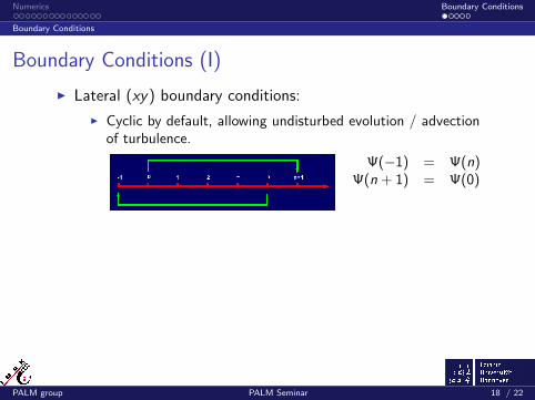
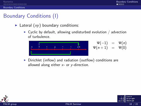
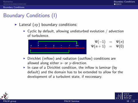
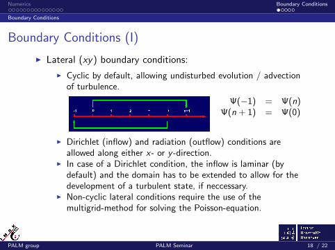
I Lateral (xy) boundary conditions:
I Cyclic by default, allowing undisturbed evolution / advectionof turbulence.
Ψ(−1) = Ψ(n)Ψ(n + 1) = Ψ(0)
I Dirichlet (inflow) and radiation (outflow) conditions areallowed along either x- or y -direction.
I In case of a Dirichlet condition, the inflow is laminar (bydefault) and the domain has to be extended to allow for thedevelopment of a turbulent state, if neccessary.
I Non-cyclic lateral conditions require the use of themultigrid-method for solving the Poisson-equation.
PALM group PALM Seminar 18 / 22
Numerics Boundary Conditions
Boundary Conditions
Boundary Conditions (I)
I Lateral (xy) boundary conditions:
I Cyclic by default, allowing undisturbed evolution / advectionof turbulence.
Ψ(−1) = Ψ(n)Ψ(n + 1) = Ψ(0)
I Dirichlet (inflow) and radiation (outflow) conditions areallowed along either x- or y -direction.
I In case of a Dirichlet condition, the inflow is laminar (bydefault) and the domain has to be extended to allow for thedevelopment of a turbulent state, if neccessary.
I Non-cyclic lateral conditions require the use of themultigrid-method for solving the Poisson-equation.
PALM group PALM Seminar 18 / 22
Numerics Boundary Conditions
Boundary Conditions
Boundary Conditions (II)
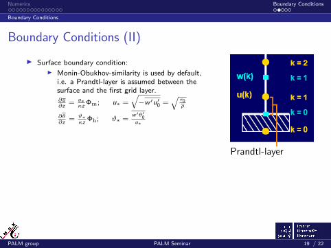
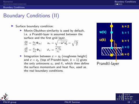
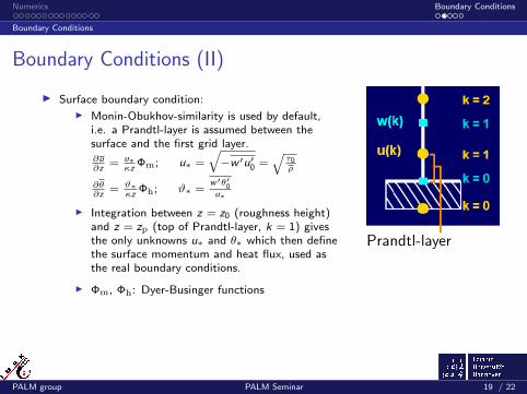
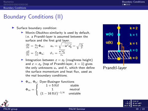
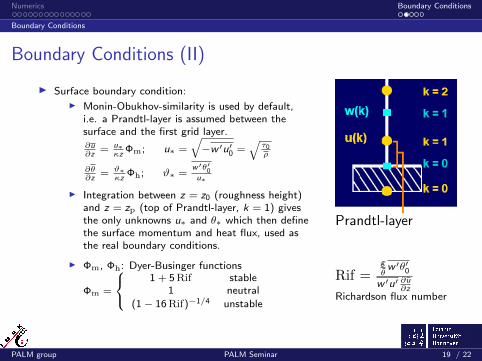
I Surface boundary condition:I Monin-Obukhov-similarity is used by default,
i.e. a Prandtl-layer is assumed between thesurface and the first grid layer.∂u∂z
= u∗κz
Φm; u∗ =√−w ′u′0 =
√τ0ρ
∂θ∂z
= ϑ∗κz
Φh; ϑ∗ =w′θ′0u∗
I Integration between z = z0 (roughness height)and z = zp (top of Prandtl-layer, k = 1) givesthe only unknowns u∗ and θ∗ which then definethe surface momentum and heat flux, used asthe real boundary conditions.
I Φm, Φh: Dyer-Businger functions
Φm =
1 + 5Rif stable
1 neutral
(1− 16Rif)−1/4 unstable
Prandtl-layer
Rif =g
θw ′θ′0
w ′u′ ∂u∂z
Richardson flux number
PALM group PALM Seminar 19 / 22
Numerics Boundary Conditions
Boundary Conditions
Boundary Conditions (II)
I Surface boundary condition:I Monin-Obukhov-similarity is used by default,
i.e. a Prandtl-layer is assumed between thesurface and the first grid layer.∂u∂z
= u∗κz
Φm; u∗ =√−w ′u′0 =
√τ0ρ
∂θ∂z
= ϑ∗κz
Φh; ϑ∗ =w′θ′0u∗
I Integration between z = z0 (roughness height)and z = zp (top of Prandtl-layer, k = 1) givesthe only unknowns u∗ and θ∗ which then definethe surface momentum and heat flux, used asthe real boundary conditions.
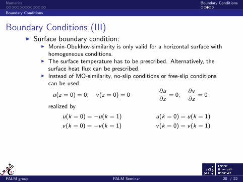
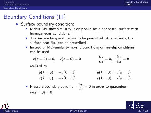
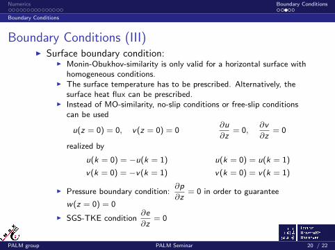
I Monin-Obukhov-similarity is only valid for a horizontal surface withhomogeneous conditions.
I The surface temperature has to be prescribed. Alternatively, thesurface heat flux can be prescribed.
I Instead of MO-similarity, no-slip conditions or free-slip conditionscan be used
u(z = 0) = 0, v(z = 0) = 0∂u
∂z= 0,
∂v
∂z= 0
realized by
u(k = 0) = −u(k = 1) u(k = 0) = u(k = 1)
v(k = 0) = −v(k = 1) v(k = 0) = v(k = 1)
I Pressure boundary condition:∂p
∂z= 0 in order to guarantee
w(z = 0) = 0
I SGS-TKE condition∂e
∂z= 0
PALM group PALM Seminar 20 / 22
Numerics Boundary Conditions
Boundary Conditions
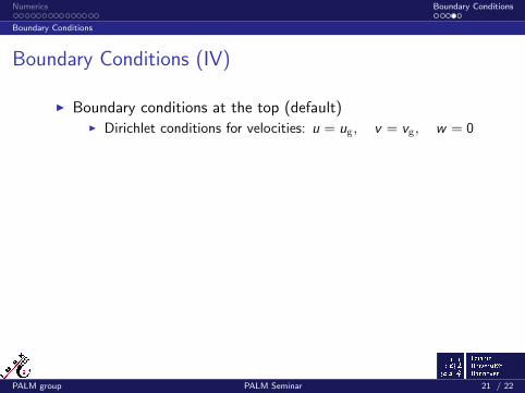
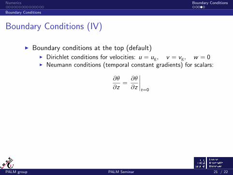
Boundary Conditions (IV)
I Boundary conditions at the top (default)I Dirichlet conditions for velocities: u = ug, v = vg, w = 0
I Neumann conditions (temporal constant gradients) for scalars:
∂θ
∂z=
∂θ
∂z
∣∣∣∣t=0
I Pressure: Dirichlet p = 0 ( Neumann∂p
∂z= 0 is better )
I SGS-TKE: Neumann∂e
∂z= 0
I A damping layer can be switched on in order to absorb gravitywaves.
PALM group PALM Seminar 21 / 22
Numerics Boundary Conditions
Boundary Conditions
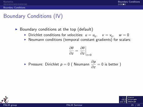
Boundary Conditions (IV)
I Boundary conditions at the top (default)I Dirichlet conditions for velocities: u = ug, v = vg, w = 0I Neumann conditions (temporal constant gradients) for scalars:
∂θ
∂z=
∂θ
∂z
∣∣∣∣t=0
I Pressure: Dirichlet p = 0 ( Neumann∂p
∂z= 0 is better )
I SGS-TKE: Neumann∂e
∂z= 0
I A damping layer can be switched on in order to absorb gravitywaves.
PALM group PALM Seminar 21 / 22
Numerics Boundary Conditions
Boundary Conditions
Boundary Conditions (IV)
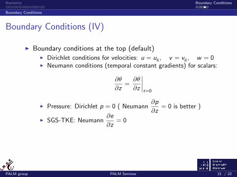
I Boundary conditions at the top (default)I Dirichlet conditions for velocities: u = ug, v = vg, w = 0I Neumann conditions (temporal constant gradients) for scalars:
∂θ
∂z=
∂θ
∂z
∣∣∣∣t=0
I Pressure: Dirichlet p = 0 ( Neumann∂p
∂z= 0 is better )
I SGS-TKE: Neumann∂e
∂z= 0
I A damping layer can be switched on in order to absorb gravitywaves.
PALM group PALM Seminar 21 / 22
Numerics Boundary Conditions
Boundary Conditions
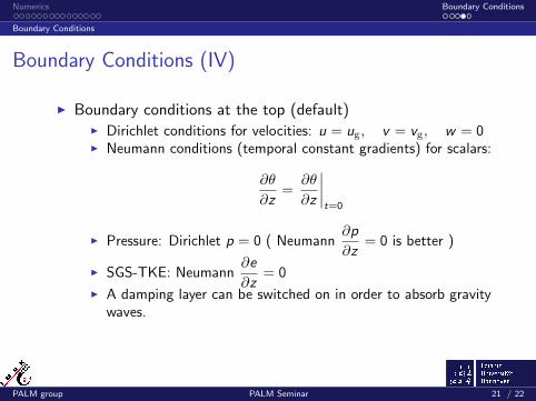
Boundary Conditions (IV)
I Boundary conditions at the top (default)I Dirichlet conditions for velocities: u = ug, v = vg, w = 0I Neumann conditions (temporal constant gradients) for scalars:
∂θ
∂z=
∂θ
∂z
∣∣∣∣t=0
I Pressure: Dirichlet p = 0 ( Neumann∂p
∂z= 0 is better )
I SGS-TKE: Neumann∂e
∂z= 0
I A damping layer can be switched on in order to absorb gravitywaves.
PALM group PALM Seminar 21 / 22
Numerics Boundary Conditions
Boundary Conditions
Initial Conditions
All 3D-arrays are initialized with vertical profiles (horizontallyhomogeneous).
Two different profiles can be chosen:
I constant (piecewise linear) profiles
I e.g. u = 0, v = 0,∂θ
∂z= 0 up to z = 1000m,
∂θ
∂z= +1.0 up to top
I velocity profiles calculated by a 1D-model (which is apart of PALM)
I constant (piecewise linear) temperature profile is used for the1D-model
Under horizontally homogeneous initial conditions, randomfluctuations have to be added in order to generate turbulence!
PALM group PALM Seminar 22 / 22
Numerics Boundary Conditions
Boundary Conditions
Initial Conditions
All 3D-arrays are initialized with vertical profiles (horizontallyhomogeneous).
Two different profiles can be chosen:I constant (piecewise linear) profiles
I e.g. u = 0, v = 0,∂θ
∂z= 0 up to z = 1000m,
∂θ
∂z= +1.0 up to top
I velocity profiles calculated by a 1D-model (which is apart of PALM)
I constant (piecewise linear) temperature profile is used for the1D-model
Under horizontally homogeneous initial conditions, randomfluctuations have to be added in order to generate turbulence!