24 Chapter 3 NURBS-based Discrete Element Method The two major components of the proposed NURBS-based DEM are the use of NURBS for representing particle geometries, and the contact algorithm for determining the signed gap or penetration between two non-convex NURBS surfaces. We discuss these two components in detail in this chapter. 3.1 Non-Uniform Rational Basis-Splines (NURBS) Non-Uniform Rational Basis-Splines (NURBS) are ubiquitous in the world of computer graphics, computer-aided design (CAD), computer-aided engineering (CAE), and computer- aided manufacturing (CAM) systems, as well as in computer animations. These functions provide great flexibility in representing arbitrary and complex geometries with much less information than conventional faceted or polynomial counterparts. Perhaps more impor- tantly, in the context of this work and as shown in this section, the mathematical properties of NURBS make them ideal candidates for the description of grain morphology, the inte- gration of discrete equations of motion, and the detection of contact. In what follows we briefly describe the essential components of NURBS in the context of the current application. The literature on NURBS is extensive and relatively mature, and our purpose here is not to present all of its elements but rather those that are needed for completeness of presentation. For an exhaustive description of NURBS the reader is referred to [48; 84–86], whose presentation and notational convention we follow closely. We adhere to the convention in the computational geometry literature where the degree
Transcript
24
Chapter 3
NURBS-based Discrete ElementMethod
The two major components of the proposed NURBS-based DEM are the use of NURBS for
representing particle geometries, and the contact algorithm for determining the signed gap
or penetration between two non-convex NURBS surfaces. We discuss these two components
in detail in this chapter.
3.1 Non-Uniform Rational Basis-Splines (NURBS)
Non-Uniform Rational Basis-Splines (NURBS) are ubiquitous in the world of computer
graphics, computer-aided design (CAD), computer-aided engineering (CAE), and computer-
aided manufacturing (CAM) systems, as well as in computer animations. These functions
provide great flexibility in representing arbitrary and complex geometries with much less
information than conventional faceted or polynomial counterparts. Perhaps more impor-
tantly, in the context of this work and as shown in this section, the mathematical properties
of NURBS make them ideal candidates for the description of grain morphology, the inte-
gration of discrete equations of motion, and the detection of contact.
In what follows we briefly describe the essential components of NURBS in the context
of the current application. The literature on NURBS is extensive and relatively mature,
and our purpose here is not to present all of its elements but rather those that are needed
for completeness of presentation. For an exhaustive description of NURBS the reader is
referred to [48; 84–86], whose presentation and notational convention we follow closely.
We adhere to the convention in the computational geometry literature where the degree
25
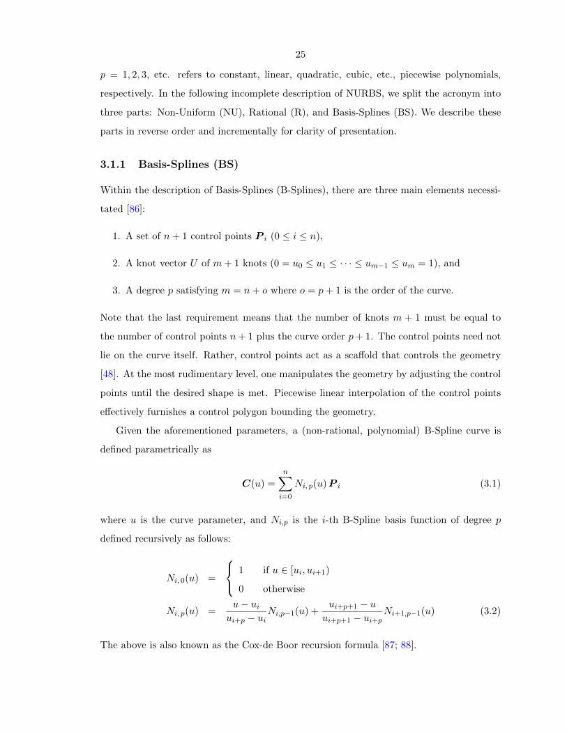
p = 1, 2, 3, etc. refers to constant, linear, quadratic, cubic, etc., piecewise polynomials,
respectively. In the following incomplete description of NURBS, we split the acronym into
three parts: Non-Uniform (NU), Rational (R), and Basis-Splines (BS). We describe these
parts in reverse order and incrementally for clarity of presentation.
3.1.1 Basis-Splines (BS)
Within the description of Basis-Splines (B-Splines), there are three main elements necessi-
tated [86]:
1. A set of n+ 1 control points P i (0 ≤ i ≤ n),
2. A knot vector U of m+ 1 knots (0 = u0 ≤ u1 ≤ · · · ≤ um−1 ≤ um = 1), and
3. A degree p satisfying m = n+ o where o = p+ 1 is the order of the curve.
Note that the last requirement means that the number of knots m + 1 must be equal to
the number of control points n+ 1 plus the curve order p+ 1. The control points need not
lie on the curve itself. Rather, control points act as a scaffold that controls the geometry
[48]. At the most rudimentary level, one manipulates the geometry by adjusting the control
points until the desired shape is met. Piecewise linear interpolation of the control points
effectively furnishes a control polygon bounding the geometry.
Given the aforementioned parameters, a (non-rational, polynomial) B-Spline curve is
defined parametrically as
C(u) =n∑
i=0
Ni, p(u)P i (3.1)
where u is the curve parameter, and Ni,p is the i-th B-Spline basis function of degree p
defined recursively as follows:
Ni, 0(u) =
1 if u ∈ [ui, ui+1)
0 otherwise
Ni, p(u) =u− ui
ui+p − uiNi,p−1(u) +
ui+p+1 − uui+p+1 − ui+p
Ni+1,p−1(u) (3.2)
The above is also known as the Cox-de Boor recursion formula [87; 88].
26
3.1.2 Rational B-Splines (RBS)
A known limitation of (non-rational) B-Splines, as defined in equation (3.1), is their inability
to capture conic sections (e.g., circles and ellipses). This limitation stems from the simple
polynomial form of B-Splines. To be able to represent conic sections, the parametric form
would need to be rational, i.e., the quotient of two polynomials. A rational B-Spline (RBS)
is furnished by adding a weight wi ≥ 0, which provides an additional degree of freedom for
geometry manipulation. Hence, the curve equation becomes
C(u) =
∑ni=0Ni, p(u)wiP i∑ni=0Ni, p(u)wi
(3.3)
=n∑
i=0
Ri, p(u)P i (3.4)
where Ri, p (u) = Ni, p (u)wi/ (∑n
i=0Ni, p (u)wi), 0 ≤ i ≥ n, are the rational basis functions.
Since Ri, p (u) is rational, the exact description of conic sections becomes possible. Naturally,
when all weights are equal to unity, equation (3.4) reduces to equation (3.1).
It is interesting to note the geometric contribution of the weights. The weight wk
affects the effective contribution of control point P k on the overall shape of the curve C(u).
Making wk smaller corresponds to ‘pushing’ the curve away from the control point P k. In
the extreme, when wk = 0, the term wkP k is annihilated from the equation of the curve
and the contribution of the control point is obviously nullified. Another interesting extreme
is obtained by making wk very large relative to other weights. Dividing equation (3.4) by
wk gives
C(u) =
∑ni 6=kNi, p(u)wi/wkP i +Nk, p(u)P k∑n
i 6=kNi, p(u)wi/wk +Nk, p(u)(3.5)
where one can see that as wk is increased, the curve C(u) is ‘pulled’ towards the control
point P k.
Remark 3.1.1 In the context of grain modeling, the inability of non-rational B-Splines to
represent conic sections should not be viewed as a disadvantage, since real grains are rarely
spherical or circular in section. NURBS can be used in their simpler polynomial B-spline
Figure 3.1: Schematic illustration of a NURBS curve. The curve degree p is 3 (cubic). Theknots ui and weights wj are listed in the vectors U and w, respectively. The kink in thecurve is due to full multiplicity k = p = 3, in which the knot/parameter value u = 0.75 isrepeated p = 3 times.
3.1.3 Non-Uniform (NU) Rational B-Splines (NURBS)
The NU portion in NURBS is furnished by the knots in the knot vector U of the B-Splines.
The non-decreasing knots ui, i = 0, 1, ...,m partitions the parameter space into segments
of half-open intervals [ui, ui+1), which are also called knot spans. The knot span can be of
zero length since the knots need not be distinct, i.e., they can be repeated. The number of
times a knot value repeats itself is called multiplicity k. Based on the way the knots are
spaced, we can divide B-Splines into the following types:
1. Uniform B-Splines, which can be subdivided into non-periodic and periodic
2. Non-uniform B-Splines
In non-periodic uniform B-Splines, the knots are uniformly spaced except at the ends
where the knot values are repeated p+ 1 times, so that
U = 0, 0, . . . , 0︸ ︷︷ ︸p+1
, up+1, . . . , um−p−1, α, α, . . . , α︸ ︷︷ ︸p+1
(3.6)
The above knots are also referred to as non-periodic or open knots. Non-periodic B-Splines
are infinitely continuously differentiable in the interior of a knot span, and (p − k)-times
continuously differentiable at a knot. If k = p, we say that the knot has full multiplicity;
the multiplicity cannot be greater than the degree. Multiplicity of knots provides a way to
specify the continuity order between segments. For example, a full multiplicity knot in the
28
knot vector (away from the ends) means that a kink or cusp is present in the curve. On
the other hand, in periodic B-Splines, the knots are uniformly spaced but the first and last
knots are not duplicated, so that the knot vector looks like
U = 0, 1, . . . , n (3.7)
Periodic B-Splines are everywhere (p− 1)-times continuously differentiable.
If the knots are unequally spaced, the knot vector is non-uniform, we get non-uniform
B-Splines (the NU part in NURBS). The non-uniformity in knots can cause the degree
p of the curve to be different between knot spans. As a matter of terminology and in
describing grain geometries, knot vectors can be defined in either [0, 1] or [0, n]. The choice
of normalization does not have any effect on the shape of the curve, and it is therefore
inconsequential. A schematic of a NURBS curve is shown in Figure 3.1.
Remark 3.1.2 Equation (3.3) is usually taken as the definition of NURBS, although the
non-uniformity of the knots is not obvious from this expression.
Remark 3.1.3 Several NURBS CAD technologies, such as Rhino [89], which are already
available for geometric design of engineering components could be directly integrated into
the modeling pipeline, facilitating the transition from binary data to models of granular
assemblies.
Remark 3.1.4 It is rare that one would work with NURBS models directly in paramet-
ric space. In practice, grain shapes are typically generated interactively or through some
optimization procedure such as least squares.
3.1.4 Closing a NURBS curve
To reproduce grain geometries accurately, it is necessary to close the NURBS curves used
to describe the grain boundary. There are at least two procedures to close a NURBS curve.
In the first procedure, closed NURBS curves are defined by ‘wrapping’ control points. In
this process, a uniform knot sequence of m+ 1 knots is constructed such that: u0 = 0, u1 =
1/m, u2 = 2/m, . . . , um = 1. Note that the domain of the curve is [up, un−p]. Then, the first
and last p control points are wrapped so that P 0 = P n−p+1 = P n−p+2, . . . ,P p−2 = P n−1
29
and P p−1 = P n. By wrapping the control points, Cp−1 continuity is ensured at the joining
point C(up) = C(un−p).
In the second approach, the first and last control points are made coincident, i.e., P 0 =
P n and the first and last p+1 knots are clamped, i.e., repeated. The curve may or may not
have Ck continuity depending on how the first and last k internal knot spans are chosen,
and the first and last k + 1 weights and control points are chosen. Perhaps the simplest
example is that of a unit circle in which the control points and weights shown in Table 3.1
are used together with the following knot vector:
U = 0, 0, 0, 1, 1, 2, 2, 3, 3, 4, 4, 4 (3.8)
We notice that P 0 = P 8 and the first and last three knot values are clamped. Also,
there are three pairs of internal knots with multiplicity two. In general, this would lead
to a loss of continuity in the first derivative. However, in this case, continuity in the
first derivative is maintained by three collinear control points in each of the following sets:
P 7,P 0 = P 8,P 1, P 1,P 2,P 3, P 3,P 4,P 5, and P 5,P 6,P 7. In this work, we will
use knot vectors that are clamped.
i xi yi wi0 1 0 1
1 1 1√
2/22 0 1 1
3 -1 1√
2/24 -1 0 1
5 -1 -1√
2/26 0 -1 1
7 1 -1√
2/28 1 0 1
Table 3.1: Control points (xi, yi) and weights wi for a unit circle.
30
3.1.5 NURBS surfaces
In 3D, we describe the grain geometry as a tensor product surface, with the coordinates of
the NURBS surface in real space given by components of the vector:
Y (u, v) =m∑
i=0
n∑
j=0
(wijNi,p(u)Nj,p(v)∑m
g=0
∑nh=0wghNg,p(u)Nh,p(v)
)P ij (3.9)
where P ij are the control points, wij are the weights, and Ni,p(u) and Nj,p(v) are the B-
Splines univariate basis functions of degree p. We must therefore specify a knot vector for
the u basis functions, and a second knot vector for the v basis functions. Although there
is no restriction on the choice of degree, we have restricted to NURBS surfaces of (cubic)
degree p = 3 in our applications.
3.1.6 Relevance of NURBS to DEM calculations
To conclude this section, some of the advantages of using NURBS in the context of DEM
calculations are listed. Some of the most salient mathematical properties of NURBS that
make them ideal candidates for DEM calculations are [48; 84]:
1. Local support property
2. Invariance under affine transformations
3. Strong convex hull property
4. Local curvature equation
5. Integration with isogeometric analysis
The local support property affords the method tremendous flexibility in the description
of grain geometries. For example, in the case of NURBS curves, local support implies that
the basis function Ni,p(u) is non-zero on [ui, ui+p+1). Since the basis function Ni,p(u) is the
coefficient of control point P i, the product Ni,p(u)P i changes if P i changes, but the change
in Ni,p(u)P i only affects the segment on [ui, ui+p+1), leaving the rest of the curve C(u)
unchanged. Therefore, because of local support, a change in the position of a control point
only affects the local portion of the NURBS curve, and this allows great flexibility when
trying to approximate grain boundaries accurately. Also, by the local support property,
31
any modifications to the weights wi, too, will only affect the section of the NURBS curve
on the [ui, ui+p+1) interval.
The invariance property of NURBS under affine transformations is useful when updating
the grains described using NURBS within the time integration scheme. Exploiting this
property, a grain’s position is updated by simply translating and/or rotating the control
points relative to the grain’s centroid.
The strong convex hull property ensures that, for a closed NURBS curve, the entire
grain is located within the convex hull defined by the corresponding control points. Us-
ing the control points to define a convex hull bounding each grain, the granular entities
described using NURBS can be easily incorporated into existing DEM global collision de-
tection algorithms. We note that the control polygon defined by the control points could
be non-convex. Also, the convex hull property fails for negative weights in which a portion
of the affected curve segment will be outside of the convex hull defined by the correspond-
ing control points. However, negative weights are not typically used when describing grain
shapes, and therefore convex hull failure is typically not a concern.
NURBS provides a simple procedure for evaluating local curvatures. It is well known
that contact stresses (e.g., Hertzian contact) depend on the radii of curvature of two con-
tacting bodies. Evaluation of curvature for simple shapes such as circles and ellipses is
straightforward but becomes complicated for arbitrary-shaped grains. In addition to pro-
viding the tangent and normal boundary vectors needed for contact force calculations,
NURBS also provide local curvature evaluations that can be used directly in calculating
local contact forces. After obtaining the first and second local derivatives C(1) and C(2),
respectively, the curvature vector can be evaluated such that
κ =
(C(1) ·C(1)
)C(2) −
(C(1) ·C(2)
)C(1)
(C(1) ·C(1)
)2 (3.10)
and consequently, the local radius of curvature is calculated such that R = 1/‖κ‖.Finally, the use of NURBS provides a foundation for high-fidelity physics at the granular
level. Since NURBS have recently been shown to furnish a basis for isogeometric analysis
[48], within each particle more complex analysis, such as plasticity, damage, or possibly
breakage, can be performed. Evidently, NURBS can offer tremendous flexibility in repre-
32
senting and optimizing grain morphology, as well as provide important geometric properties
that would enable higher-fidelity discrete calculations.
Remark 3.1.5 Isogeometric analysis is a computational mechanics technology that uses ba-
sis functions emanating from computer aided geometric design (CAGD), such as B-splines,
NURBS, and T-splines. It has been shown that isogeometric analysis provides more precise
and efficient geometric representations [48].
Remark 3.1.6 The last two of the above features of NURBS have not been considered in
this thesis. These can potentially be explored in the future.
3.2 Contact Problem and Implementation
Our earlier work described in [49; 50] has focused on particles geometries that are angular
but strictly convex, and the contact algorithms were generalizations of the intersection-based
approach used for disks and spheres. While the work has led to improvements in particle
morphology representation beyond disks and spheres, it was still limited in two ways. First,
the increase in rolling resistance of angular but convex geometries relative to disks is limited.
For instance, rolling resistance provided by distributed contact reaction over flat boundaries
cannot be represented using strictly convex shapes. Moreover, interlocking behavior between
non-convex particles, which contributes significantly to mobilized strength and stability
[90; 91], is not accounted for. Second, the generation of strictly convex NURBS shapes is
very difficult and restrictive from a modeling perspective. This is even more so when dealing
with image data of real particle shapes and obtaining strictly convex boundaries through a
fitting procedure is not possible in most cases.
A contact algorithm capable of dealing with general non-convex NURBS particles, to
be described in this chapter, would eliminate the above two limitations. As a result, a
more faithful representation on the contact force distributions over particle boundaries is
obtained and the image data-to-analysis pipeline is significantly streamlined. Without loss
of generality, we will work with 3D NURBS surfaces throughout the remaining of this
chapter. We also assume that the underlying parametric domain has been normalized, i.e.,
0 ≤ u ≤ 1 and 0 ≤ v ≤ 1 (a unit square).
33
3.2.1 General definition
Potential contact I
Slave
Master
n
X
Y
x y
z
∂Ωi
∂Ωj
Ωj
Ωi
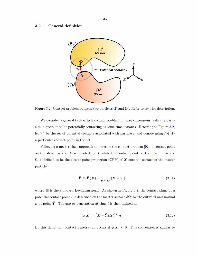
Figure 3.2: Contact problem between two particles Ωi and Ωj . Refer to text for description.
We consider a general two-particle contact problem in three dimensions, with the parti-
cles in question to be potentially contacting at some time instant t. Referring to Figure 3.2,
let Wi be the set of potential contacts associated with particle i, and denote using I ∈ Wi
a particular contact point in the set.
Following a master-slave approach to describe the contact problem [92], a contact point
on the slave particle Ωj is denoted by X while the contact point on the master particle
Ωi is defined to be the closest point projection (CPP) of X onto the surface of the master
particle:
Y ≡ Y (X) = minY ∈ ∂Ωi
‖X − Y ‖ (3.11)
where ‖‖ is the standard Euclidean norm. As shown in Figure 3.2, the contact plane at a
potential contact point I is described on the master surface ∂Ωi by the outward unit normal
n at point Y . The gap or penetration at time t is then defined as
g(X) =[X − Y (X)
]Tn (3.12)
By this definition, contact penetration occurs if g(X) < 0. This convention is similar to
34
that used in the definition of contact problems in the finite element method (FEM) [92]. In
the context of classic DEM [24] with a linear contact law, once the gap is determined, the
normal contact force on the master particle is then calculated as (refer to (2.1)):
f =
kNg(X)n, if g(X) < 0
0, otherwise
(3.13)
where kN is the normal contact stiffness. An equal and opposite force acts on the slave
particle. Essentially, the contact problem boils down to the problem of solving the CPP
problem (3.11) and in the remaining sections, we describe how this is done in the context
of NURBS.
3.2.2 Knot positioning
We generalize the node-to-surface approach typically used in the contact treatment of finite
element models [92] to a ‘knot-to-surface’ (KTS) approach to enable the contact treatment
of non-convex particles described using NURBS surfaces. More recently, the KTS approach
has been employed in isogeometric finite elements [93] and a similar approach is taken
here. The contact points X associated with the slave particle are represented through
knots and these points are to be projected onto the master surface to determine if there
is contact penetration. The representation of contact points through knots is necessary for
computational tractability, as well as for tracking the incremental slip and contact gain or
loss around non-convex surfaces of potentially contacting particles. While similar to nodal
discretization in FEM, we emphasize that the key difference here is that the positioning of
contact points by knots does not change the particle geometry, i.e., isogeometric; the knots
vary continuously in the underlying parametric space. In this work, we have adopted to
position the knots a priori as a preprocessing step.
In real applications where a large number of arbitrary-shaped grains are represented by
3D NURBS surfaces, the manual positioning of knots proved to be extremely difficult, if
not impossible. As such, an automatic and adaptive knot positioning strategy is required.
To this end, we have devised an automatic knot positioning algorithm based on a NURBS
recursive subdivision scheme (see Algorithm 2). The NURBS surface is subdivided until
the following termination criteria (see Figure 3.3) are met:
35
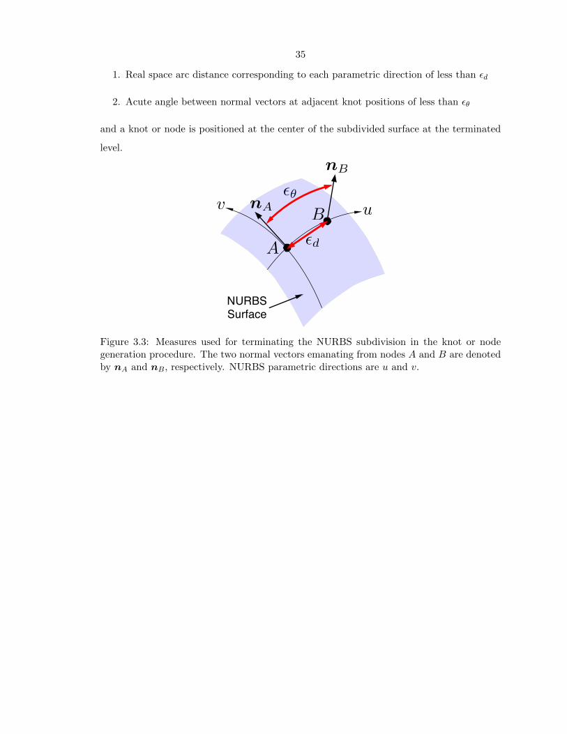
1. Real space arc distance corresponding to each parametric direction of less than εd
2. Acute angle between normal vectors at adjacent knot positions of less than εθ
and a knot or node is positioned at the center of the subdivided surface at the terminated
level.
d
uv
A
BnA
nB
NURBS Surface
Figure 3.3: Measures used for terminating the NURBS subdivision in the knot or nodegeneration procedure. The two normal vectors emanating from nodes A and B are denotedby nA and nB, respectively. NURBS parametric directions are u and v.
36
Input: NURBS surface S = Y (u, v), real arc distance tolerance εd, angle tolerance εθOutput: List of knot positions in real space
procedure AKP(S)Calculate the real-space points corresponding to the corners in parametric space:x1 = x(umin, vmin), x2 = x(umax, vmin), x3 = x(umax, vmax), x4 = x(umin, vmax)
Calculate real arc distance corresponding to each parametric direction:Du = max(‖x3 − x4‖, ‖x1 − x2‖), Dv = max(‖x1 − x4‖, ‖x2 − x3‖)
Define acute angle between unit normal vectors θ(n1,n2) = cos−1 (n1 · n2)
if ( Du > Dv )∗ then
Compute unit normal vectors: nu1 = n(umin + ∆u/3, vave),nu2 = n(umin + 2∆u/3, vave) and θu = θ(nu1,nu2).
if ( Du > εd ) and ( θu > εθ ) thenSplit surface into 2 child surfaces S1, S2 at uave
elseSurface is a LEAF
end if
else ( Du ≤ Dv )∗
Compute unit normal vectors: nv1 = n(uave, vmin + ∆v/3),nv2 = n(uave, vmin + 2∆v/3) and θv = θ(nv1,nv2).
if ( Dv > εd ) and ( θv > εθ ) thenSplit surface in into 2 child surfaces S1, S2 at vave
elseSurface is a LEAF
end if
end if
if ( Surface is a LEAF ) thenStore midpoint x(uave, vave) as a knot position
elseRecurse, i.e., apply AKP, on the two child surfaces S1, S2
end ifend procedure
∗For a closed single patch NURBS surface, a seam joins either the edges at (a) u = 0, 1or (b) v = 0, 1. At first entry into this procedure, the if (Du > Dv) block is executed forcase (a) while the if (Du ≤ Dv) block is executed for case (b).
The distance function of a fixed slave point X on a slave surface to a master surface Y (u, v)
is given by
d(u, v) = ‖X − Y (u, v)‖ (3.14)
or, squaring both sides, we obtain the distance squared function
f(u, v) = [X − Y (u, v)]T [X − Y (u, v)] (3.15)
where f(u, v) = [d(u, v)]2 and the coordinates of the NURBS surface Y (u, v) is given by
(3.9).
The CPP problem can then be formulated as (cf. (3.11))
Y = min(u,v)∈Γ
f(u, v) (3.16)
where Γ is the bounded normalized parametric space of the NURBS master surface. In real
applications, where surfaces are always well-defined, the underlying NURBS basis functions
are products or quotients (with denominators that are bounded away from zero) of uni-
variate B-Splines basis functions, which in turn are polynomials. This implies the distance
squared function f(u, v) is Lipschitz continuous. This means that there exists a finite bound
on the rate of change of the squared distance function. This key observation allows one to
employ the Lipschitzian dividing rectangle (DIRECT) global optimization procedure as a
solution to the CPP problem.
3.2.4 The DIRECT optimization algorithm
Here, we describe how the DIRECT algorithm can be adapted to the CPP problem (3.16).
We describe the following two components of the DIRECT algorithm,
1. Sample and subdivide
2. Identification of potentially optimal parametric rectangles
followed by a simple example to illustrate how the overall DIRECT algorithm works. We
emphasize that, in the application of this algorithm, the NURBS surface or underlying
38
parametric domain is not physically subdivided. The key feature of the DIRECT algorithm
is that the subdivisions are performed implicitly through sampling (i.e., function evaluation)
and selection of optimal rectangles.
3.2.4.1 Sample and subdivide
The basic idea of this step is as follows: the sampling part determines the goodness of
the current solution of f in (3.16), while the subdivision part ensures efficiency as well
as convergence of the DIRECT algorithm. After subdivision, the parametric domain will
consist of subregions that are either squares or rectangles. We first describe the sample and
subdivide step for squares followed by an extension to rectangles.
The basic idea behind the DIRECT algorithm is the sampling of the values of the
function f at the points c ± δei, i = 1, 2, where c is the center of the parametric square,
δ is one-third side length of the parametric square, and ei is the unit vector in either the
u (i = 1) or v (i = 2) direction. Since the underlying parametric domain of the NURBS
surface is 2D, the sampling points would be located above, below, to the left, and to the
right of the center point (see Figure 3.4(a) or (b)).
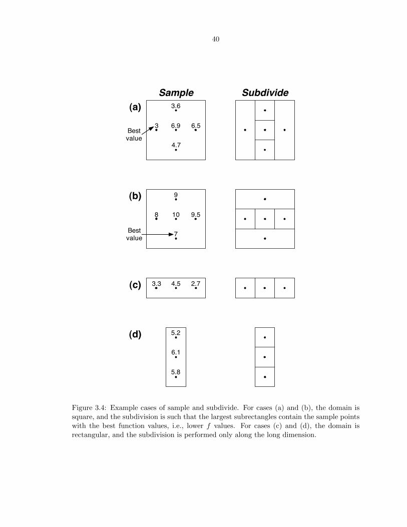
The square domain is subdivided such that each subregion (rectangle or square) would
contain a sample point at its center. The following strategy for subdividing the square is
adopted in [94]. Let
wi = min f(c− δei), f(c+ δei) , i ∈ 1, 2 (3.17)
be the best of the function values sampled along the u and v directions. First, split the
square into thirds along the dimension with the smallest w value. Then, split the rectangle
that contains c into thirds along the remaining direction. This strategy ensures that the
largest subrectangle contains the sample point with the best function value, i.e., lowest f
value. The reason for this strategy is to bias the search near points with good function
values, since larger rectangles are preferred for sampling (as a result of convex hull; see be-
low). For rectangular domains, the subdivision is performed only along the long dimension.
This ensures that the rectangles shrink in both parametric directions, ensuring convergence
[94]. Examples illustrating this subdivision strategy are shown in Figure 3.4. Algorithm 3
formally describes the above steps and covers both square and rectangular domains.
39
Input: A parametric subregion (rectangle or square)Output: A subdivided subregion
1: Identify the set I ⊆ 1, 2 with maximum parametric side length in parametric space,where 1 and 2 are in the u and v directions, respectively. Let δ equal to one-third ofthis maximum length (if square, pick both sides, otherwise pick longer dimension - seeexplanation in the text).
2: Sample the function at the points c± δei for all i ∈ I, where c is the center of theparametric rectangle and ei is the i-th unit vector.
3: Divide the rectangle containing c into thirds along the dimensions in I, starting withthe dimension lowest value of
wi = min f(c− δei), f(c+ δei)and continue to the next dimension.
Algorithm 3: Sample and Subdivide Algorithm
40
Sample
10 9.58
9
7
Subdivide
6.9 6.53
3.6
4.7
4.5 2.73.3
(a)
(b)
(c)
(d) 5.2
6.1
5.8
Best value
Best value
Figure 3.4: Example cases of sample and subdivide. For cases (a) and (b), the domain issquare, and the subdivision is such that the largest subrectangles contain the sample pointswith the best function values, i.e., lower f values. For cases (c) and (d), the domain isrectangular, and the subdivision is performed only along the long dimension.
41
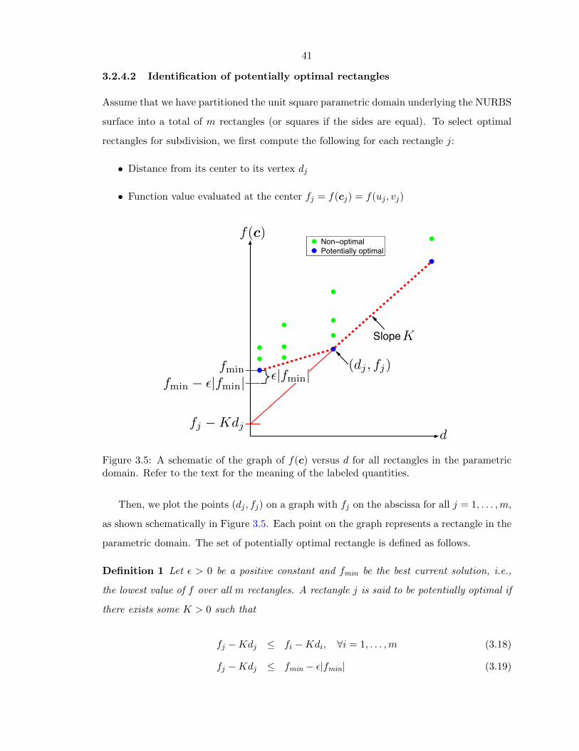
3.2.4.2 Identification of potentially optimal rectangles
Assume that we have partitioned the unit square parametric domain underlying the NURBS
surface into a total of m rectangles (or squares if the sides are equal). To select optimal
rectangles for subdivision, we first compute the following for each rectangle j:
• Distance from its center to its vertex dj
• Function value evaluated at the center fj = f(cj) = f(uj , vj)
Non−optimalPotentially optimal
f(c)
d
fmin
fmin − |fmin| |fmin| (dj , fj)
Slope K
fj − Kdj
Figure 3.5: A schematic of the graph of f(c) versus d for all rectangles in the parametricdomain. Refer to the text for the meaning of the labeled quantities.
Then, we plot the points (dj , fj) on a graph with fj on the abscissa for all j = 1, . . . ,m,
as shown schematically in Figure 3.5. Each point on the graph represents a rectangle in the
parametric domain. The set of potentially optimal rectangle is defined as follows.
Definition 1 Let ε > 0 be a positive constant and fmin be the best current solution, i.e.,
the lowest value of f over all m rectangles. A rectangle j is said to be potentially optimal if
there exists some K > 0 such that
fj −Kdj ≤ fi −Kdi, ∀i = 1, . . . ,m (3.18)
fj −Kdj ≤ fmin − ε|fmin| (3.19)
42
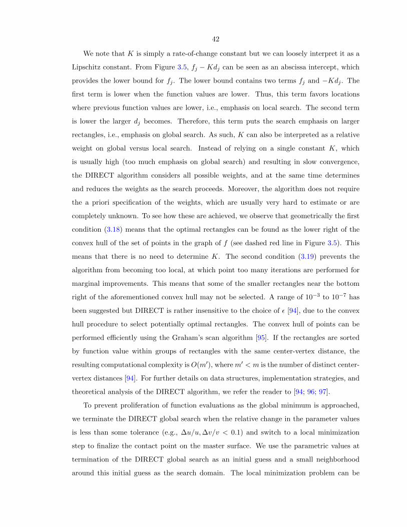
We note that K is simply a rate-of-change constant but we can loosely interpret it as a
Lipschitz constant. From Figure 3.5, fj −Kdj can be seen as an abscissa intercept, which
provides the lower bound for fj . The lower bound contains two terms fj and −Kdj . The
first term is lower when the function values are lower. Thus, this term favors locations
where previous function values are lower, i.e., emphasis on local search. The second term
is lower the larger dj becomes. Therefore, this term puts the search emphasis on larger
rectangles, i.e., emphasis on global search. As such, K can also be interpreted as a relative
weight on global versus local search. Instead of relying on a single constant K, which
is usually high (too much emphasis on global search) and resulting in slow convergence,
the DIRECT algorithm considers all possible weights, and at the same time determines
and reduces the weights as the search proceeds. Moreover, the algorithm does not require
the a priori specification of the weights, which are usually very hard to estimate or are
completely unknown. To see how these are achieved, we observe that geometrically the first
condition (3.18) means that the optimal rectangles can be found as the lower right of the
convex hull of the set of points in the graph of f (see dashed red line in Figure 3.5). This
means that there is no need to determine K. The second condition (3.19) prevents the
algorithm from becoming too local, at which point too many iterations are performed for
marginal improvements. This means that some of the smaller rectangles near the bottom
right of the aforementioned convex hull may not be selected. A range of 10−3 to 10−7 has
been suggested but DIRECT is rather insensitive to the choice of ε [94], due to the convex
hull procedure to select potentially optimal rectangles. The convex hull of points can be
performed efficiently using the Graham’s scan algorithm [95]. If the rectangles are sorted
by function value within groups of rectangles with the same center-vertex distance, the
resulting computational complexity is O(m′), wherem′ < m is the number of distinct center-
vertex distances [94]. For further details on data structures, implementation strategies, and
theoretical analysis of the DIRECT algorithm, we refer the reader to [94; 96; 97].
To prevent proliferation of function evaluations as the global minimum is approached,
we terminate the DIRECT global search when the relative change in the parameter values
is less than some tolerance (e.g., ∆u/u,∆v/v < 0.1) and switch to a local minimization
step to finalize the contact point on the master surface. We use the parametric values at
termination of the DIRECT global search as an initial guess and a small neighborhood
around this initial guess as the search domain. The local minimization problem can be
43
solved using either gradient-based or derivative-free constrained optimization algorithms
[98]. Here, we choose the derivative-free procedure since it is simpler and does not require
the evaluation of the Hessian of the function f .
3.2.5 Implementation of contact algorithm
The implementation of the CPP operation can be simply achieved by programming a func-
tion handle that returns the squared distance value f between a given slave contact point X
and a point Y (u, v) on the master surface, and using this function handle in the DIRECT
algorithm. The CPP algorithm proceeds as described in Algorithm 4. The one-to-one
mapping of the DIRECT algorithm to the CPP problem is particularly noteworthy; except
for a few quantities that are relevant to NURBS and the CPP problem, the steps proceed
identically with those laid out in [94]. An illustration of the DIRECT algorithm for a few
iterations is shown in Figure 3.6. The proposed contact algorithm is then implemented by
applying the CPP algorithm on candidate contact pointsX of the slave surface to determine
their closest projected points Y (X). The penetration is calculated using (3.12), from which
the corresponding normal contact force vector on the master particle is then determined by
(3.13).
The identification of candidate slave contact points for the CPP operation can be per-
formed through a number of standard collision detection algorithms (e.g., [42]). For ex-
ample, only those points that are inside the bounding box of the master surface will be
considered.
44
Input: Slave point X and master surface Y (u, v)Output: Closest projected point Y (X)
1: Let c1 = (u1, v1) be the center point of normalized parameter space (unit square) andevaluate f(c1). Set current best value fmin = f(c1), number of sample points m = 1,and iteration counter k = 0.
2: Identify the set S of potentially optimal parametric rectangles.
3: Select any rectangle j ∈ S.
4: Sample and subdivide (see Algorithm 2). Update fmin and m = m+ ∆m where ∆m isthe number of new points sampled.
5: Remove rectangle j from set S. If S is not empty, go to Step 3.
6: Increment iteration counter k = k + 1. If relative in parametric direction is less thanspecified tolerance, go to Step 7. Otherwise, go to Step 2.
7: Start constrained optimization procedure using current best (u, v) and correspondingparametric rectangle to finalize the closest projected point on the master surface Y (X).Exit.
Algorithm 4: DIRECT Closest Point Projection Algorithm
Figure 3.6: Illustration of DIRECT algorithm. For simplicity, we have set ε in (3.19) tozero. The lines are only to guide the eye — there is no physical subdivision of the NURBSsurface or underlying parametric surface; instead the subdivision is performed implicitlythrough sampling and selection of optimal rectangles.
46
3.3 Closure
We have presented a new algorithm for determining the signed gap value for non-convex
NURBS surfaces. The functionality of the algorithm will be demonstrated through discrete