NX MAGNETICS - TUTORIALS COUPLED ELASTICITY Dr. Binde Ingenieure March 31, 2022 2011-2022 Dr. Binde Ingenieure, Design & Engineering GmbH. All Rights Reserved. This software and related documentation are proprietary to Dr. Binde Ingenieure, Design & Engi- neering GmbH. All other trademarks are the property of their respective owners. DR. BINDE INGENIEURE, DESIGN & ENGINEERING GMBH MAKES NO WARRANTY WHATSOEVER, EXPRESSED OR IMPLIED THAT THE PROGRAM AND ITS DOCUMEN- TATION ARE FREE FROM ERRORS AND DEFECTS. IN NO EVENT SHALL DR. BINDE INGENIEURE, DESIGN & ENGINEERING GMBH BECOME LIABLE TO THE USER OR ANY PARTY FOR ANY LOSS, INCLUDING BUT NOT LIMITED TO, LOSS OF TIME, MONEY OR GOODWILL, WHICH MAY ARISE FROM THE USE OF THE PROGRAM AND ITS DOCUMENTATION. THIS SIMULATION SOFTWARE USES FINITE ELEMENT METHODS. USERS SHOULD BE AWARE THAT RESULTS CAN HAVE UNPREDICTABLE ERRORS IF INPUT DATA IS NOT COMPLETELY CORRECT. THEREFORE ANY DESIGN DECISIONS SHOULD NOT BE BASED SOLELY ON THE SIMULATION. USE ADDITIONAL MEASUREMENTS TO ENSURE THE CORRECTNESS. 1
Transcript
NX MAGNETICS - TUTORIALS COUPLEDELASTICITY
Dr. Binde Ingenieure
March 31, 2022
2011-2022 Dr. Binde Ingenieure, Design & Engineering GmbH. All Rights Reserved. Thissoftware and related documentation are proprietary to Dr. Binde Ingenieure, Design & Engi-neering GmbH. All other trademarks are the property of their respective owners.
DR. BINDE INGENIEURE, DESIGN & ENGINEERING GMBH MAKES NO WARRANTYWHATSOEVER, EXPRESSED OR IMPLIED THAT THE PROGRAM AND ITS DOCUMEN-TATION ARE FREE FROM ERRORS AND DEFECTS. IN NO EVENT SHALL DR. BINDEINGENIEURE, DESIGN & ENGINEERING GMBH BECOME LIABLE TO THE USER ORANY PARTY FOR ANY LOSS, INCLUDING BUT NOT LIMITED TO, LOSS OF TIME,MONEY OR GOODWILL, WHICH MAY ARISE FROM THE USE OF THE PROGRAMAND ITS DOCUMENTATION.
THIS SIMULATION SOFTWARE USES FINITE ELEMENT METHODS. USERS SHOULDBE AWARE THAT RESULTS CAN HAVE UNPREDICTABLE ERRORS IF INPUT DATA ISNOT COMPLETELY CORRECT. THEREFORE ANY DESIGN DECISIONS SHOULD NOTBE BASED SOLELY ON THE SIMULATION. USE ADDITIONAL MEASUREMENTS TOENSURE THE CORRECTNESS.
1
Contents
1 Introduction 4
2 Recommended Settings 52.1 Set Site and User Material Libraries . . . . . . . . . . . . . . . . . . . . . . . . . 52.2 Use Polygon Body Names for Meshes and Physicals . . . . . . . . . . . . . . . . 52.3 Use High Resolution for Polygon Bodies . . . . . . . . . . . . . . . . . . . . . . 62.4 Create Non-manifold Polygon Bodies . . . . . . . . . . . . . . . . . . . . . . . . 6
This guide shows different problems with electromagnetic elasticity coupling and their corre-sponding simulations. The electromagnetic part is solved using the Magnetics solver. Theelasticity part is either solved by Magnetics and it’s integrated elasticity solver or by SimcenterNastran.
4
2 Recommended Settings
To simplify the work, we recommend to change the following settings.
2.1 Set Site and User Material Libraries
We recommend to reference the two material libraries (the one that comes with Magnetics andthe that comes with Simcenter MAGNET) for easier access in the customer defaults. (findit here: File, Utilities, Customer Defaults, Gateway, Materials/Mass, Locations) To have easyaccess to both libraries, without the need to browse for the files each time, set the folders asfollows (see picture below):
• ’Site and User Material Library Format’: ’Directory of MatML Files’
• At ’Directory Name’, ’Windows’, set for one of them
or a corresponding folder depending on the NX/Simcenter installation.
• Set the other to
’C:/Program Files/Siemens/NX1980/MAGNETICS/’
or a corresponding folder depending on the NX/Simcenter installation.
2.2 Use Polygon Body Names for Meshes and Physicals
If the NX/Simcenter version is 1899 (2020.1) or higher, we recommend to enable the followingsetting in the customer defaults (find it here: File, Utilities, Customer Defaults. Then: Simula-tion, Pre-Post, Meshing, General) named ’Use polygon body names for 3D meshes’.
5
When this setting is active, the names of the polygon bodies will be transferred to meshes, meshcollectors and physical property tables. Thus, the feature ’Auto Rename’ from the Magneticstoolbar becomes (nearly) obsolete. It is much easier to work, when bodies, meshes, collectorsand physicals are identically named and therefore, we recommend this setting.
2.3 Use High Resolution for Polygon Bodies
We recommend to set the standard resolution of polygon bodies to ’High’ because this oftensimplifies meshing of complex geometries.(find it here: File, Utilities, Customer Defaults. Then:Simulation, Pre-Post, General, FE Model Create)
2.4 Create Non-manifold Polygon Bodies
If the NX/Simcenter version is 1953 (2021.1) or higher, we recommend to enable an early accessfeature (find it here, see picture below: File, Utilities, Early Access Feature), named ’Allowupdates related to Electro Magnetics’. Set this ’On’.
6
Since version 2008 (2022.1), this feature is named ’Create Non-manifold Polygon Bodies’ and itis now found in the customer defaults. (find it here, see picture below: File, Utilities, CustomerDefaults, Simulation, Pre/Post, General, FE Model Create, Create Non-manifold Polygon Bod-ies, Allow)
With this feature being activated, Mesh Mating Conditions (MMC) become obsolete. Instead ofMMCs, the system will internally and fully automatic find all adjacent faces of the solid bodiesand match them. For checking, there will be a group named ’non-manifold face’ that can beselected to see all the faces that are matched.
7
More technical spoken, if there are two adjacent faces found, the system will remove one of themand use the remaining face for both solids. Thus, the result is the same as one would get withMMCs, but that new internal process is much more robust. Therefore, we recommend to usethis new feature even if it is still categorized ’Early Access’. The face matching is done whenthe Fem file is created. It can be seen and checked through the group ’non-manifold face’ thatholds all matched faces.
One disadvantage of this feature is that pyramid transitions between hex and tetrahedral el-ements are currently not possible. So, tetra elements are directly connected to hex and theinterface will have one element edge without connection. Tests have shown that in low frequencyelectromagnetic simulations, nearly no loss in accuracy results from that missing connection.
8
3 Deforming Conductor
In this example we want to analyse for the elastic deformations that result from magnetic forces.A conductor is positioned in a magnetic field resulting from two permanent magnets. For check-ing purposes we first create a static solution and compare the Lorentz forces against theory.
In a time domain analysis we assign a half sinus current running through the conductor andsolve for the Lorentz forces that result. The Lorentz forces on the conductor are computed forevery time step and can be post processed as graph or plot.
There follows a transient dynamic elasticity analysis to find the conductors deformations, stressesand reaction forces. First we use the internal elasticity solver that is delivered with Simcenter/NXMagnetics. Because the solver is internally this process is very easy. Alternatively to the inter-nal elasticity solver we also want to solve by Simcenter/NX Nastran. We apply fixed boundaryconditions and import a file that contains the Lorentz forces. As result we get deformations andstresses.
Estimated time: 1.5 h.
Follow the steps:
3.1 Analysis of Magnetic Forces
1. Open the file ’DeformingConductor.prt’ from the folder’Tutorials/8.CouplStructural/8.1DeformingConductor/start’.
9
2. Start Simcenter Pre/Post, Create a ’New Fem and Simulation’, use Solver MAGNETICSand Analysis Type ’3D Electromagnetics’. Switch off the ’Create Idealized Part’.
• Create a first Solution of Type ’Magnetostatics’ and name it ’MagSta1’. (For checkingpurposes we first create a static solution.)
• In the Output Requests under box ’Plot’ activate ’Nodal Force - virtual’ and ’LorentzForce’ and under box ’Table’ activate ’Total Force - virtual’ and ’Total Lorentz Force’.You can also activate other types you are interested in. Click Apply.
• Create a second Solution of Type ’Magnetodynamic Transient’ and name it ’Mag-Dyn1’.
• Activate again the ’Plot’ output requests ’Nodal Force - virtual’ and ’Lorentz Force’.This is for viewing the forces in the plot.
• Additionally activate again in the ’Table’ box ’Total Force - virtual’ and ’Total LorentzForce’
• and in box ’4D Fields’ also activate ’Force-virtual, NodeID Table’. Here, at ’TimeDelay’ insert -0.0001 s. This setting will shift the magnetic forces by one time step.This way Nastran will activate the forces at the same time as Magnetics does.
10
• Hint: The virtual energy method is a more complete analysis of forces since it alsocaptures reluctance forces and those forces that result from permanent magnets. Suchare not included in Lorentz forces, because Lorentz forces compute the vector productof electric current and magnetic flux density.
• In the Time Steps you set the ’Number of Time Steps’ to 50 and the ’Time Increment’to 0.0001 s.
• Hint: The conductor has a natural frequency at 235 Hz. You can check this by a NXNastran Solution 103. Because 1/235Hz = 0.004s our current will force the conductorto vibrate in natural frequency.
• Click OK
3. Switch to the Fem file
• Create automatic mesh mating conditions. There should be 16 conditions created.
• Mesh the conductor using hex elements. (Tet elements also work). Choose the sug-gested element size divided by 2, and 30 layers. Prior to meshing, set mesh controlson the four edges and force the mesh to include four elements in the section of theconductor (see picture below).
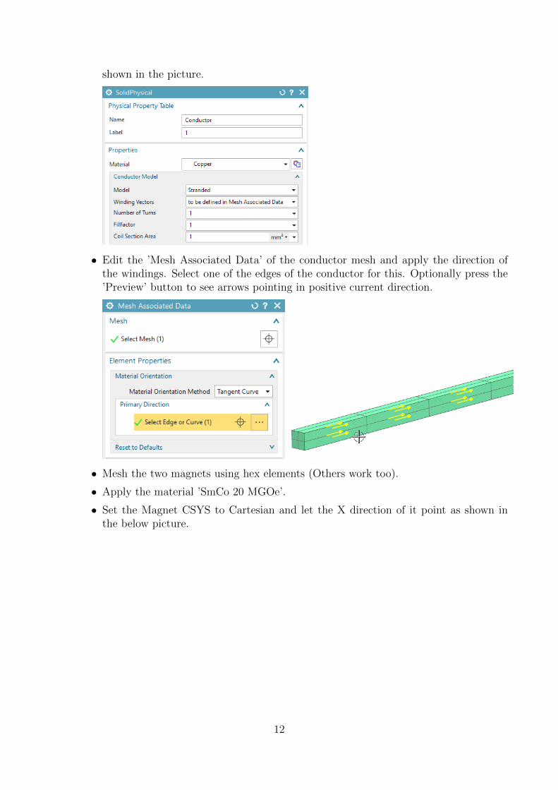
• Name the mesh collector ’Conductor’ and assign material ’Copper’ from the libraryto the conductor. Set the ’Conductor Model’ to ’Stranded’ and use the settings as
11
shown in the picture.
• Edit the ’Mesh Associated Data’ of the conductor mesh and apply the direction ofthe windings. Select one of the edges of the conductor for this. Optionally press the’Preview’ button to see arrows pointing in positive current direction.
• Mesh the two magnets using hex elements (Others work too).
• Apply the material ’SmCo 20 MGOe’.
• Set the Magnet CSYS to Cartesian and let the X direction of it point as shown inthe below picture.
12
• Mesh the air volume using tets and the half of the suggested element size. Apply thebutton ’Transition with Pyramid Elements’ if you used hex before.
• Apply a ’FluidPhysical’ and ’Air’ material to this mesh collector.
• Because we want to exclude from the force computation all bodies but the conductorwe must check the id labels of the Magnets physicals. We find they have id 2. Wewill use this in a following step in the Sim file.
• Select the button ’Rename Meshes and Physicals by Collectors’ from toolbar ’Mag-
netics’ . All meshes and Physicals will be renamed and post processing will besimplified.
4. Switch to the Sim file.
• Edit solution ’MagDyn1’, in register ’Output Requests’ box ’More’ at ’No Force Phys-ical IDs’ assign 2 because we do not want force results on the magnets.
13
• Create a constraint ’Flux tangent (zero a-Pot)’ on all 6 faces of the air volume. Alsoapply this to the two small electrode faces of the conductor. Apply this constraint toboth solutions.
• Activate the static solution andCreate a load of type ’Current’, use the default type ’On Stranded Coil’. Select theConductor physical. Insert an ’Electric Current’ of 100 A.
• Activate the dynamic solution andCreate a load of type ’Current’, use the default type ’On Stranded Coil’. Select theConductor physical and set the ’Method’ to ’Harmonic’. Insert an ’Electric Current’of 100 A, a ’Frequency’ of 235 Hz (remember, this is near the natural frequency) and aPhase Shift of 90 deg. (The Phase Shift changes the default cosines type load to sinus).
14
5. Solve both solutions
6. Notice that after the dynamic solution has completed, there is a new text file ’Deforming-Conductor1 sim1-MagDyn1.NodeIdForceVirt.txt’ in the working folder. This file containsthe force that will later be transferred to NX Nastran elasticity analysis. Notice also there isa batch file in the same folder, named ’DeformingConductor sim1-MagDyn1.CreateNastranInc.bat’.This batch must be executed to convert the text file into the format that can be includedinto Nastran.
7. In the working folder, double click that batch file (’*.CreateNastranInc.bat’). There willbe a file ’.inc’ created. This inc file contains in Nastran syntax FORCE entries assignedto nodes and to time steps. The DLOAD ID is set to 3000. We will later include this filein the Nastran input file.
8. Postprocess the static force results.
• Open the results for the static solution and display the x component of the result’LorentzForce’. (The same can be done for the virtual forces, witch are named ’Force’.Both results are very near.)
• Blank the Air mesh and all 2D meshes.
15
• Set the Color Display to ’Arrows’.
• you should see a picture like below.Hint: Depending on your current direction the direction of the force may be flipped.
• To calculate the sum of all forces acting on the conductor you can now compute the
sum of the element forces using the ’Identify Results’ function :
• Use the ’Identify Results’ function and set the ’Pick’ to ’Mesh’. Select the conductormesh and find the sum is about 0.3 N.
9. A analytical solution for the lorentz force on the conductor can be found as follows:−→FL = q(~v × ~B) = I(~̀× ~B)withI = 100A,B = 0.03T, ` = 0.1mthe lorentz force results toFL = 0.3NThough, the result from our simulation is close to this value.
10. Post process the dynamic solution as you like.
11. Save your parts. Don’t close them.
16
3.2 Internal Elasticity Solver Usage
The internal elasticity solver can handle 3D and 1D elements. Tetra and hexa elements are bydefault solved by second order nodal shape functions. Instead of mid nodes the elasticity solveruses the element edges and faces, so result quality is high and similar to NX Nastran second orderhexa and tetra elements. Also pyramids and wedges are possible, but in first order only, so beaware that these elements are not very accurate. Also there are 1D rod elements available. Thesolver can be used for static and transient dynamic solutions. There is no nonlinear capabilityavailable. Following we set up the deforming conductor model to use this internal elasticitysolver.
1. Set the Fem file to the displayed part.
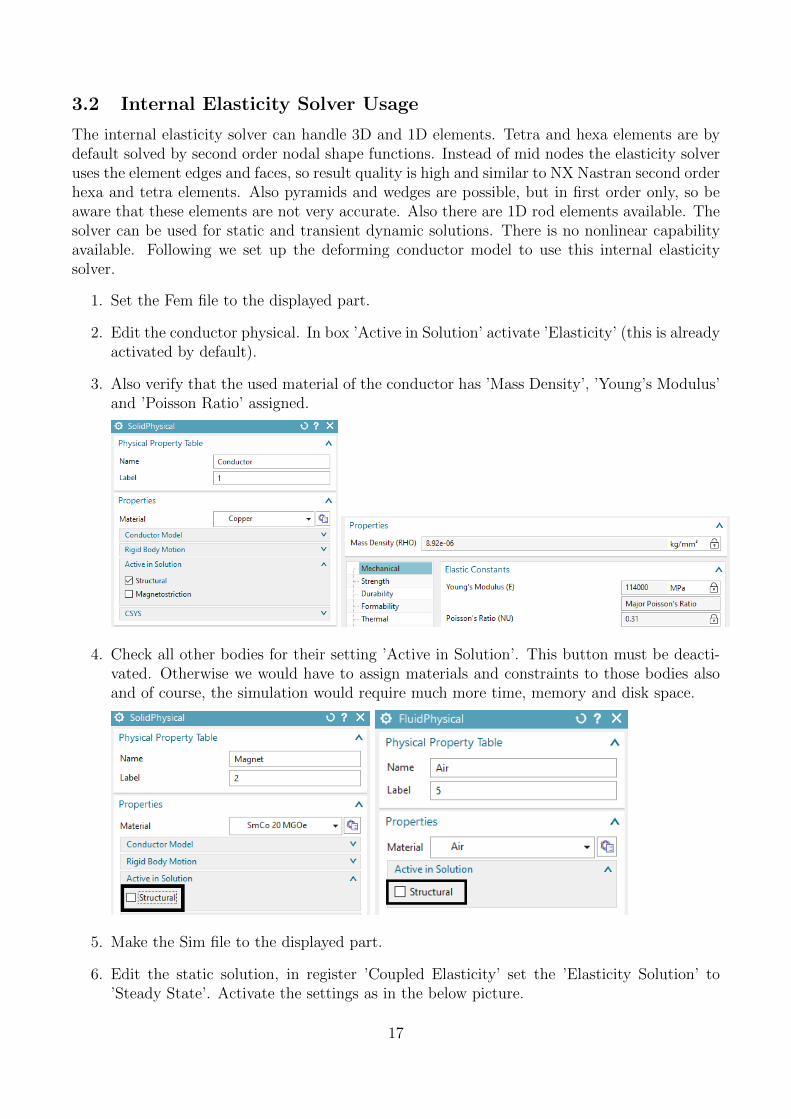
2. Edit the conductor physical. In box ’Active in Solution’ activate ’Elasticity’ (this is alreadyactivated by default).
3. Also verify that the used material of the conductor has ’Mass Density’, ’Young’s Modulus’and ’Poisson Ratio’ assigned.
4. Check all other bodies for their setting ’Active in Solution’. This button must be deacti-vated. Otherwise we would have to assign materials and constraints to those bodies alsoand of course, the simulation would require much more time, memory and disk space.
5. Make the Sim file to the displayed part.
6. Edit the static solution, in register ’Coupled Elasticity’ set the ’Elasticity Solution’ to’Steady State’. Activate the settings as in the below picture.
17
7. Edit the transient solution, in register ’Coupled Elasticity’ set the ’Elasticity Solution’ to’Transient’. Activate the settings as in the below picture.
8. Create a constraint of type ’EM Elasticity Constraint’, set the type to ’On Edges’ and selectthe two edges of the conductor as shown below. These edges will allow the conductor todeform easily because rotation is allowed. Set all degrees of freedom to ’Fixed’ and pressOK.
9. Create a second ’EM Elasticity Constraint’ on on edge of the other side of the conductor.Fix only the x and y directions here.
18
10. Assign these two constraints to both solutions. Later we will also assign these constraintsto the Nastran solution.
11. Solve both solutions
12. Post processing: The deformation (left) and von Mises stress (right) result of the staticsolution are shown in the below picture.
13. The maximum deformation over time (blue) and the force (red) from the transient solutionare shown in the picture below. Both curves are in the AFU file, because they have beenrequested in the tabular output requests of the dynamic solution.
19
3.3 Transfer Magnetic Forces to Nastran Solver
We will now create a copy of the Fem and Sim files for the following Nastran elasticity analysis.Notice that in this analysis it is necessary to use the same node ID numbers as in the electromag-netic analysis. It is possible to add meshes. It is also possible to add mid nodes to the existingmesh for better stress results (we will do this here). Only it is not allowed to remove nodes orelements. In this case we will use a Nastran solution 109 to include transient dynamical effects.Other Nastran solution types would also work corresponding to their capabilities. The resultswill match with those from the previous section where the internal elasticity solver of Magneticswas used. The advantage of using Nastran is in many additional functions (contact, nonlinearmaterials, ...) that Nastran can handle.
1. Make a copy of the Fem and Sim files. Therefore, first save the files,
2. then set the Fem file to the displayed part,
3. Do a ’Save As’ and assign the name ’DeformingConductor fem2.fem’
4. The system also asks for a new Sim file. Key in ’DeformingConductor sim2.sim’.
5. A ’Save As’ window appears. Press ’Yes’.
6. In the Fem file:
• Edit the FEM file and set the Solver to NX/Simcenter Nastran, OK.
20
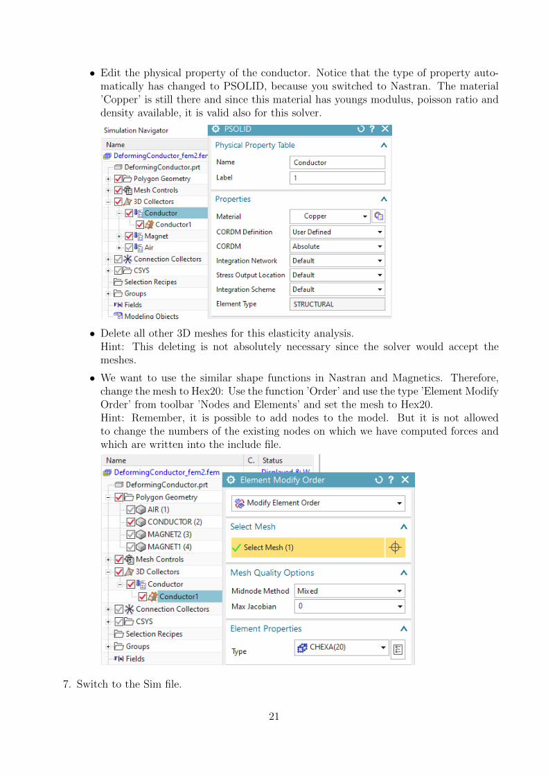
• Edit the physical property of the conductor. Notice that the type of property auto-matically has changed to PSOLID, because you switched to Nastran. The material’Copper’ is still there and since this material has youngs modulus, poisson ratio anddensity available, it is valid also for this solver.
• Delete all other 3D meshes for this elasticity analysis.Hint: This deleting is not absolutely necessary since the solver would accept themeshes.
• We want to use the similar shape functions in Nastran and Magnetics. Therefore,change the mesh to Hex20: Use the function ’Order’ and use the type ’Element ModifyOrder’ from toolbar ’Nodes and Elements’ and set the mesh to Hex20.Hint: Remember, it is possible to add nodes to the model. But it is not allowedto change the numbers of the existing nodes on which we have computed forces andwhich are written into the include file.
7. Switch to the Sim file.
21
8. Optionally delete the two existing solutions ’MagSta1’ and ’MagDyn1’ and also the oldloads. Keep the constraints because we can use them here.
9. Create a new solution of type 109 with solver Simcenter Nastran and name it ’StrDyn1’,(other transient NX Nastran solution types are also possible) Click OK.
10. in the following dialogue ’Solution Step’ create a modeling object for ’Time StepInterval’. Set the ’Number of Time Steps’ to 50 and the ’Time Increment’ to 0.0001 s.
Click OK. Add the newly created Time Step object to the list . Click Close and OK.
11. To add the magnetic forces, witch reside in the text file with extension ’inc’, proceed asfollows:
• Edit the solution. In the case control section, create a modeling object for ’Userdefined Text’. At ’Keyin Text’ insert ’DLOAD=3000’. This is the group of electro-magnetic forces that will be included.
22
• In register ’Bulk Data’: Again create a modeling object for ’User Defined Text’.
Key in the text line that points to the include file for forces:
include ’DeformingConductor sim1-MagDyn1.NodeIdForceVirt.inc’
Click Ok, Ok.
12. Because the force units in the include file are written in mN we have to check that theseunits are used by the Nastran solution also. Edit the Advanced Solver Options (RMBon solution) of this solution and switch to register General. Ensure that the Output FileUnits are set to (mN)(mm)(Kg).
13. Reuse the two constraints that were used for the electromagnetic analysis with deformation.
23
14. Solve the solution and postprocess the results.
• Display the displacement result of the first Increment.
• Set deformation to ’Absolute’ and ’Scale’ to 25. Activate ’Show undeformed model’
• Create an animation over the iterations. It should be seen a deformation that resultsfrom magnetic forces (picture below left).
• Picture below right shows a comparison of the maximum x displacement between theNastran (red) and the Magnetics (blue) solver results. The deviations between theresults of the two solvers are considerably small.
24
15. Save your parts and close them.
3.4 Thermal Expansion
The effect of thermal expansion can be added to the model. Therefore, temperatures must alsobe considered. Temperatures can either be computed by a coupled thermal solution or applied asfixed value. In this tutorial we will compute them. They result from the current in the conductor.More details on coupled thermal solutions can be found in the corresponding tutorial document’Tutorials Coupled Thermal’. Here we will apply such temperatures together with the previouslydiscussed Lorentz forces and expect a slightly larger deformation of the conductor.
1. open again the file from the previous section ’DeformingConductor sim1.sim’ and
2. set the Fem file to the displayed part.
3. When using the given material properties and current value for the conductor there wouldbe only a very small additional deformation visible in this case because of very smalltemperature rise. Therefore, just to see more effect, we will increase the material property’Thermal Expansion Coefficient’ of copper by the factor 10000.
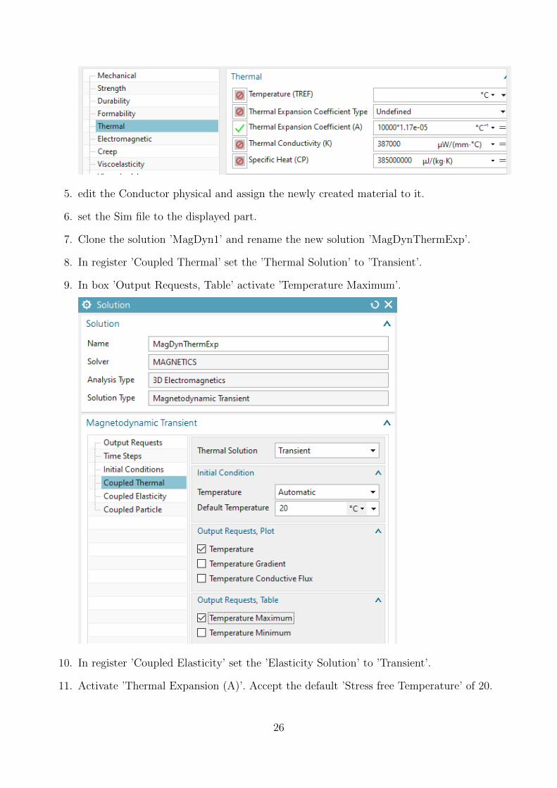
4. Make a copy of the Copper material, edit the new material and in register ’Thermal’ changethe ’Thermal Expansion Coefficient (A)’ from 1.17e-05 to 10000*1.17e-05.
25
5. edit the Conductor physical and assign the newly created material to it.
6. set the Sim file to the displayed part.
7. Clone the solution ’MagDyn1’ and rename the new solution ’MagDynThermExp’.
8. In register ’Coupled Thermal’ set the ’Thermal Solution’ to ’Transient’.
9. In box ’Output Requests, Table’ activate ’Temperature Maximum’.
10. In register ’Coupled Elasticity’ set the ’Elasticity Solution’ to ’Transient’.
11. Activate ’Thermal Expansion (A)’. Accept the default ’Stress free Temperature’ of 20.
26
12. In box ’Output Requests, Table’ activate ’Max Displacement’.
13. Click OK to finish the dialogue.
14. Create an ’EM Thermal Constraint’. Set the type to ’Free Convection’. Key in 20 degreesfor the ’Ambient Temperature’ and 2 W/(m2 ∗ C) for the ’Convection Coefficient’ (takecare of the unit). Select the four outside faces of the conductor. Click OK.
27
15. Solve the solution.
16. After solve has finished, display the graph for the maximum displacement of the conductorin x direction (’MaxStrucX Conductor’). Overlay the same graph from the previous solu-tion ’MagDyn1’. It can be seen a larger deformation in the case with thermal expansioneffect. See picture below: red curve is with thermal expansion, blue is without.
The tutorial is finished.
28
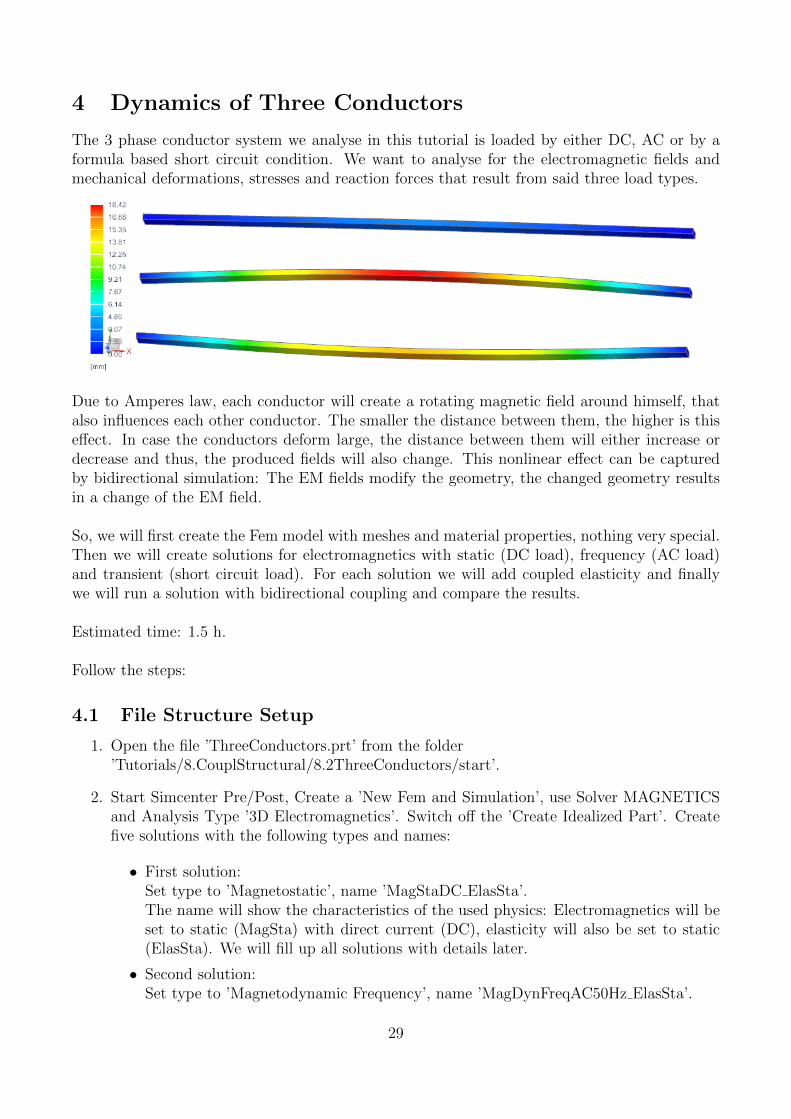
4 Dynamics of Three Conductors
The 3 phase conductor system we analyse in this tutorial is loaded by either DC, AC or by aformula based short circuit condition. We want to analyse for the electromagnetic fields andmechanical deformations, stresses and reaction forces that result from said three load types.
Due to Amperes law, each conductor will create a rotating magnetic field around himself, thatalso influences each other conductor. The smaller the distance between them, the higher is thiseffect. In case the conductors deform large, the distance between them will either increase ordecrease and thus, the produced fields will also change. This nonlinear effect can be capturedby bidirectional simulation: The EM fields modify the geometry, the changed geometry resultsin a change of the EM field.
So, we will first create the Fem model with meshes and material properties, nothing very special.Then we will create solutions for electromagnetics with static (DC load), frequency (AC load)and transient (short circuit load). For each solution we will add coupled elasticity and finallywe will run a solution with bidirectional coupling and compare the results.
Estimated time: 1.5 h.
Follow the steps:
4.1 File Structure Setup
1. Open the file ’ThreeConductors.prt’ from the folder’Tutorials/8.CouplStructural/8.2ThreeConductors/start’.
2. Start Simcenter Pre/Post, Create a ’New Fem and Simulation’, use Solver MAGNETICSand Analysis Type ’3D Electromagnetics’. Switch off the ’Create Idealized Part’. Createfive solutions with the following types and names:
• First solution:Set type to ’Magnetostatic’, name ’MagStaDC ElasSta’.The name will show the characteristics of the used physics: Electromagnetics will beset to static (MagSta) with direct current (DC), elasticity will also be set to static(ElasSta). We will fill up all solutions with details later.
• Second solution:Set type to ’Magnetodynamic Frequency’, name ’MagDynFreqAC50Hz ElasSta’.
29
Set the ’Forcing Frequency’ to 50 Hz. So, we want to use a frequency domain solutionfor electromagnetics with AC current at 50 Hz and a steady state solution for theelasticity part.
• Third solution:Set the type to ’Magnetodynamic Frequency’, name ’MagDynFreqAC50Hz ElasFreq’.Set the ’Forcing Frequency’ to 50 Hz. The extension ’ElasFreq’ means that we wantto use a frequency response elasticity solution.
• Forth solution:Set the type to ’Magnetodynamic Transient’, name ’MagDynTrans ShortCircuit’. Wewill use a transient solution for both electromagnetics and elasticity. The current willbe a short circuit type.
• Fifth solution:Set the type to ’Magnetodynamic Transient’, name ’MagDynTrans ShortCircuit BiDir’.Same as above, but we want to activate the bidirectional coupling.
4.2 Fem File Setup
1. Change the displayed part to the Fem file.
2. Create mesh mating conditions. There should be 12 such conditions created. Blank theAir polygon body.
3. Mesh the ’Conductor1’ with Hexaedral elements. Use the suggested element size (6.32mm). Activate ’Use layers’ and set the ’Number of Layers’ to 30.
4. Edit the newly created mesh collector and his Physical. Set the material to ’Copper’ fromthe Magnetics material library. Check that in the setting ’Active in Solution’ the option
30
’Elasticity’ is on.
5. In the same way create meshes and Physicals for the remaining two conductors.
6. Unblank and mesh the Air body. Use tetrahedral elements and the suggested element size(129 mm). Because of the hex, tet-transition, activate the option ’Transition with PyramidElements’.
7. For the Air mesh, create a ’FluidPhysical’ and material ’Air’ from the Magnetics materiallibrary.
8. Select the button ’Rename Meshes and Physicals by Collectors’ from toolbar ’Magnetics’
. All meshes and Physicals will be renamed and post processing will be simplified.
4.3 EM Loads Setup - DC, AC, Short Circuit
1. Change to the Sim file.
2. Blank the 3D Collectors for easier selection. Activate (double click) the ’MagStaDC ElasSta’solution.
31
3. Create a constraint of type ’Flux tangent (zero a-Pot)’ on all 9 outside faces. Also the 6electrode faces of the 3 conductors must belong to this group. This constraint must beused in all solutions, so drag-drop it into the others.
4. Create a Voltage load: Set the type to ’On Solid Face’, key in 0 V and select the 3 electrodefaces of the 3 conductors (no matter which side). This voltage load must be active in allsolutions (all but the frequency solution), so drag-drop it into the such. For the frequencysolution, create a separate one in the same way.
5. In the active solution ’MagStaDC ElasSta’, create three ’Current’ loads as follows:
• Set the type to ’On Solid Face’ and the ’Method’ to ’Harmonic’.
• For ’Electric Current Amplitude’ key in 50000 A, for ’Frequency’ 50 Hz and for ’PhaseShift’ 0 degrees.
• Select the electrode face of conductor 1. Click OK.
• Create a similar load on the second conductor with a ’Phase Shift’ 120 degrees.
• Create a similar load on the third conductor with a ’Phase Shift’ 240 degrees.
6. Activate solution ’MagDynFreqAC50Hz ElaSta’ and create three ’Current’ loads as follows:
• Set the type to ’On Solid Face’ and the ’Definition’ to ’Amplitude/Phase’.
• For ’Electric Current Amplitude’ key in 50000 A and for ’Phase Shift’ 0 degrees.
• Select the electrode face of conductor 1. Click OK.
• Create a similar load on conductor 2 with a ’Phase Shift’ 120 degrees.
• Create a similar load on conductor 3 with a ’Phase Shift’ 240 degrees.
7. Activate solution ’MagDynTrans ShortCircuit’ and create three ’Current’ loads with ana-lytical formulas to describe the exponential behaviour of a short circuit as follows:
• Set the type to ’On Solid Face’ and the ’Method’ to ’Analytic’.
• Key in the following formula:Sqrt[2] ∗ 2e4 ∗ (Sin[2 ∗ Pi ∗ 50 ∗ $Time− 1.57] + Exp[−$Time/0.0455] ∗ Sin[1.57])
• notice the 1.57 that appears two times: This describes the phase shift for the 3 phasecurrent system.
• Create a second and a third Current load on the electrodes faces of the second andthird conductors. On the second, use a phase shift of 1.57 + 2∗Pi/3 and on the thirduse 1.57 + 4 ∗ Pi/3
• Drag-drop these three analytical loads into solution ’MagDynTrans ShortCircuit BiDir’.
4.4 Elasticity Constraints Setup
1. Activate (double click) the ’MagStaDC ElasSta’ solution.
32
2. Create a ’EM Elasticity Constraint’ on the first conductor. Set the type to ’On Edges’and select the shown two edges. Set all ’Degrees of Freedom’ to ’Fixed’ and click OK.
3. For the remaining two conductors, create constraints in the same way.
4. Drag-drop the three elasticity constraints into all other solutions.
4.5 Solution: EM Static, Elasticity Static
1. Activate solution ’MagStaDC ElasSta’.
2. In register ’Output Requests’ activate results as desired.
3. In register ’Coupled Elasticity’, set the ’Elasticity Solution’ to ’Steady State’ and activatethe ’Output Requests’ as shown in the picture below.
4. Solve the solution.
5. Display the Y displacement results. The maximum is 38 mm.
33
4.6 Solution: EM Frequency, Elasticity Static
In frequency domain solutions all loads and results are assumed to be harmonic. So, all resultsoscillate between phase angle 0 (real part), angle 90 (imaginary part), 180 and 270. Therefore,also the resulting mechanical forces come out as oscillating. To use the forces in the followingelasticity solution, they are evaluated at phase angle 0.
1. Activate solution ’MagDynFreqAC50Hz ElaSta’.
2. In register ’Output Requests’ activate results as desired.
3. In register ’Coupled Elasticity’, set the ’Elasticity Solution’ to ’Steady State’ and activatethe ’Output Requests’ as shown in the picture below.
4. Solve the solution.
5. Check the resulting Y displacements. They should be very near to those from the staticsolution. The reason is that the frequency is quite low, so results are nearly static. Withhigher frequencies, skin effects would increase and results would change.
34
4.7 Solution: EM Frequency, Elasticity Frequency
1. Activate solution ’MagDynFreqAC50Hz ElaFreq’.
2. In register ’Output Requests’ activate results as desired.
3. In register ’Coupled Elasticity’, set the ’Elasticity Solution’ to ’Frequency Response (EMForces harmonic)’ and activate the ’Output Requests’ as shown in the picture below.
4. Solve the solution.
5. To check the resulting displacements, run a animation to see the oscillation. Becausedisplacements here are complex results (frequency domain) the same rules apply as forEM results in frequency domain. To animate, set in ’Post View’, register ’Deformation’the ’Complex Option’ to ’At Phase Angle’ and the ’Scale’ to 1, ’Absolute’. Then use the’Animation’, set ’Style’ to ’Modal’ and ’Full cycle’, then ’Play’.
35
6. The maximum displacements in this simulation are about 14 mm and thus much smallerthan in the previous simulation, where we had 38 mm. A reason for this can be that theexcitation frequency 50 Hz is away from the mechanical natural frequency of this conductorsystem. Such natural frequency can by found by a solve with NX Nastran solution 103.A nice additional training would be to find that natural frequency, apply the AC load atthat frequency and find the displacements then again.
4.8 Solution: EM Transient Short Circuit, Elasticity Transient
For the following two transient solutions we want to use a trick: We include the air body intothe elasticity solution. By that way the air mesh will deform smoothly, forced by the conductorsdeformations. This trick leads to a nice air mesh at each time step even if large deformationsappear (only the bidirectional solution is affected by this). Of course, the air material needsas material properties a small value for Youngs modulus, Poisson ratio and Mass density. Thevery small Youngs modulus leads to deformations, but nearly no stresses in the air, so theconductor deformations are nearly not affected by this. As a disadvantage, solve time andmemory consumption will increase, because of many more elements in the elasticity system.
1. Make the Fem part active.
2. Edit the Physical of the air and at ’Active in Solution’, activate ’Elasticity’.
3. Optionally check that the air material has said mechanical properties.
4. Make the Sim part active again.
Following we activate the elasticity solution:
1. Activate solution ’MagDynTrans ShortCircuit’.
2. In register ’Output Requests’ activate results as desired.
3. In register ’Time Steps’, set the ’Time Increment’ to 0.05/25 and the ’Number of TimeSteps’ to 25.
36
4. In register ’Coupled Elasticity’, set the ’Elasticity Solution’ to ’Transient’ and activate the’Output Requests’ as shown in the picture below.
5. Solve the solution.
6. Display the three graphs showing the maximum conductor Y displacements over time.As the following picture shows, the maximum displacement is found at conductor 2 withabout 33 mm.
4.9 Solution: EM Transient Short Circuit, Elasticity Transient, Bidi-rectional
We want to use the same settings as in the prior solution except one setting: The Bidirectionaloption will be active here.
2. In register ’Output Requests’ activate results as desired.
3. In register ’Time Steps’, set the ’Time Increment’ to 0.05/25 and the ’Number of TimeSteps’ to 25.
37
4. In register ’Coupled Elasticity’, set the ’Elasticity Solution’ to ’Transient’. Activate ’Bidi-rectional (Deforme Mesh)’. Also activate the ’Output Requests’ as shown in the picturebelow.
5. Solve the solution.
6. Display the maximum Y conductor displacements of conductor 2 of both Short Circuitsolutions. As the following picture shows, the bidirectional solution shows slightly smallerdisplacements.
7. Display the displacements at time 0.014 (maximum, as seen above). Because in thissimulation the bidirectional effect is active, now both effects are captured:
• The EM field increases the deformation,
• The increased distance leads to smaller EM fields.
The solution is more realistic: The distance between conductors 1 and 2 increases, buttherefore the fields become smaller and this again leads to a smaller distance.
38
The tutorial is finished.
39
5 Elasticity Contact
This tutorial shows how electric conductors contact while deforming. A later tutorial additionallyshows how contacts can influence the electric current, what means if a gap arises, the electricresistance becomes very large. This example only shows the mechanical effects.
Follow the steps to see how the model is set up, solved and how the contact can be managed.The tutorial starts from an existing Fem and Sim file. Only the relevant features are added.
Estimated time: 1 h.
5.1 Contact Concepts
We use a classical elasticity contact feature, also called penalty contact algorithm. That featureintroduces nonlinear mechanical effects what means that at each time step the solver mustcheck for penetration in the contact area and if such penetration appears, there will be contactforces added. The contact forces must be adjusted in a way that the penetration disappears orfalls below a given limit. To find such correct contact forces the solver must perform severaliterations. Because of these extra contact iterations the computational costs become significantlylarger when using contact.
Two contact types are possible: ’Node-to-Node Contact’ and ’Surface-to-Surface Contact’. Thefirst type can be used to define single contacts between two points in the model. The secondtype is more advanced and can also handle coulomb friction. In this example we use both typesfor completeness.
40
5.2 The Start Model
First check the existing files of the tutorial.
1. Open the file ’ElasticityContact sim1.sim’ from the folder’Tutorials/8.CouplStructural/8.3ElasticityContact/complete’
2. Delete all existing ’Simulation Objects’. These contacts will be created in the following.
3. Check the existing model:
• There are meshes of different types just to make sure contact work on all of them.
• Two solutions are already there. One will be used for face contact and one for nodecontact. The solutions are of Magnetostatic type with zero time steps and we areonly interested in the elasticity part.
• Notice there are two ’Output Requests’ activated for this contact simulation: ’ContactDistance and Slide’ and ’Contact Pressure, Friction Stress and Force’.
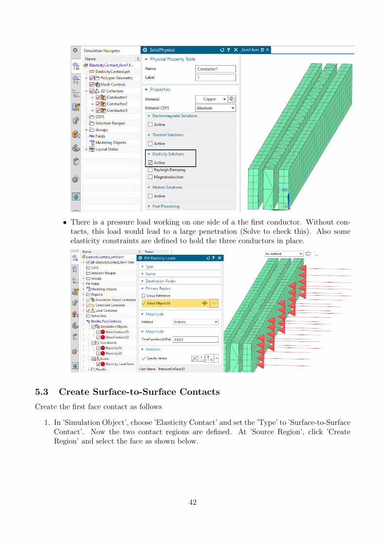
• The Physicals of all conductors also show that only the elasticity solution is of in-terest. All others are deactivated. The material is copper with an standard elasticmodulus and poisson ratio.
41
• There is a pressure load working on one side of a the first conductor. Without con-tacts, this load would lead to a large penetration (Solve to check this). Also someelasticity constraints are defined to hold the three conductors in place.
5.3 Create Surface-to-Surface Contacts
Create the first face contact as follows
1. In ’Simulation Object’, choose ’Elasticity Contact’ and set the ’Type’ to ’Surface-to-SurfaceContact’. Now the two contact regions are defined. At ’Source Region’, click ’CreateRegion’ and select the face as shown below.
42
2. At ’Target Region’, again click ’Create Region’ and select the opposing face.
3. At ’Elasticity Contact Parameters’, click ’Create Modeling Object’. The coefficient offriction, damping and several numerical parameters can be modified here. In many casesthe defaults work fine, so there is no need to change anything now. Click OK two timesto finish the contact creation.
4. Create the second contact in the same way between conductor 2 and 3 and their corre-
43
sponding faces.
5.4 Contact Parameters Overview
Even if we did not modify any, we will give a short information about the above contact pa-rameters, because they definitely influence the simulation process. Although, many models runwith the defaults, often solve time can be reduced by adjusting contact parameters.
• ’Coefficient of Friction’: This value controls the coulomb friction forces that appearif this value is set larger than zero. Such friction forces act on the two contact faces inopposing directions, depending on the relative motion (slide). To control friction, there arealso the two limits ’Displacement Limit for no Friction’ and ’Displacement Limitfor full Friction’. The assumption is that friction forces do not appear suddenly, ratherthan gradually increasing depending on the slide distance. Though, the first limit definesa small slide range that does not produce any friction forces. Then, if slide increases, therange between limit 1 and limit 2 defines the slide range in which the friction coefficientarises linearly between zero and the full given value. If slide becomes higher, full frictionstays in effect.
• ’Max Allowable Penetration’: This maximum penetration value defines the limit orresidual that must be reached for a contact to converge.
• ’Min/Max Search Distance’: The algorithm searches from the source to the targetfaces (and opposite) to find contact penetrations. These two distances define the limits ofthat search. They shouldn’t be too small because often there is large penetration at thebeginning of a contact process and even then the limits must fit.
44
• ’Initial Stiffness’ and ’Adaptive Stiffness’: The contact algorithm finds penetrationand calculates contact forces by the amount of penetration times a stiffness factor. If’Adaptive Stiffness’ is not activated, the used stiffness stays always the initial value givenhere. If the adaptive feature is activated, the stiffness factor will update depending on thecurrent contact force, penetration and on the ’Adaptive Relax Factor’.
• ’Adaptive Max Stiffness’: If the adaptive stiffness feature is used this value controlsthe maximum possible stiffness.
• ’Adaptive Min Factor’: In case gaps arise during the contact iterations, the contactpressure will not suddenly become zero, rather it will decrease depending on the ’DistanceRelax Factor’. As soon as the ’Adaptive Min Factor’ is reached, the pressure is set to zero.
• ’Adaptive Relax Factor’: This relax factor can be used to influence the adaptive stiffnesscomputation. A smaller value, e.g. 0.1 leads to smaller stiffness, a higher value, e.g. 5.leads to more aggressive stiffness increase.
• ’Adaptive Num Iterations’: This factor defines whether the adaptive stiffness is up-dated once at the beginning of a time step only (Default) or if it is updated again atfollowing iterations.
• ’Adaptive over Time’: If active, the previously adaptive stiffness is used at the beginningof a new time step. If not, it is initialized with the initial stiffness value.
• ’Distance Relax Factor’: This factor controls how aggressive stiffness is decreased ifgaps arise in contacts. Normally, the default should not be changed.
Some more settings for contact are found in the solver parameters under register ’Numeric’ inbox ’Nonlinear Elasticity Contact’. These are global settings, being valid for all contacts. Ifthe setting ’Method’ is switched from ’Program Controlled’ to ’User Set’ one can modify them.To see more info in the following simulation, we set the ’Logfile Output’ to ’All’. Following themeanings of the settings.
45
• ’Max Iterations Contact Loop’: Defines the maximum number of contact iterations.If the residuals of all contacts are not below their limits after these iterations, the wholestep has not converged.
• ’Allowed Number Not Converged Steps’: Sometimes some contact residuals do notfully reach their limit but the overall solution is valid. Therefore, this parameter defineshow many of such not converged (connected) time steps are allowed until the solutionstops. The solution monitor indicates such steps with ’NOT converged - Continue’.
• ’Intermediate Results Output’: Setting this option to ’All’ leads to a result output atall contact iterations. This can be used for debugging purposes mainly.
• ’Logfile Output’: By default this is set to ’Mini’, meaning the solution monitor showsinformation about each final contact iteration. Setting this to ’All’ results in showing eachiteration in the solution monitor.
• ’Plot Results on’. By using the default option ’One Contact-Side only’, contact resultslike pressure, force, sliding,... are shown on the first side of each contact only. Normally,the second side will have the opposing values and therefore it is not necessary to show such.Nevertheless, setting this option to ’Both Sides’ will show the results on both contact sides.
5.5 Solving and Monitoring
1. Solve this solution ’ElasSta FaceContacts’.
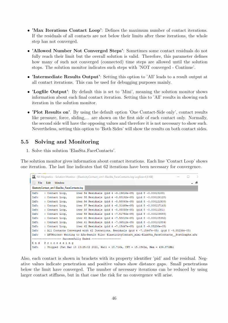
The solution monitor gives information about contact iterations. Each line ’Contact Loop’ showsone iteration. The last line indicates that 62 iterations have been necessary for convergence.
Also, each contact is shown in brackets with its property identifier ’pid’ and the residual. Neg-ative values indicate penetration and positive values show distance gaps. Small penetrationsbelow the limit have converged. The number of necessary iterations can be reduced by usinglarger contact stiffness, but in that case the risk for no convergence will arise.
46
5.6 Post Processing Contact Results
1. Open the plot results and display the result ’Displacements’. Verify that the overall solu-tion looks correct.
2. Also check the contact results. Display ’Contact Normal Force’, ’Contact Pressure’, ’Con-tact Slide’, ’Contact Distance’
5.7 Create Node-to-Node Contacts
In the second solution ’ElasSta NodeContacts’ we want to use node contacts instead of facecontacts.
1. Activate the second solution.
2. Create a new ’Simulation Object’ of ’Elasticity Contact’ and use the type ’Node-to-NodeContact’.
3. At ’Contact Node One’ select a node from the face of conductor one quite in the middle.
4. At ’Contact Node Two’ select a node from the face of conductor two quite in the middle.Click OK and the contact is created.
5. Create a second node contact between conductor two and three.
6. Solve the solution and post process the results.
47
7. Deformation results will be similar to the face contact solution.
8. When comparing stress results, a difference is found. Because the node contact (picturebelow right) loads all contact forces on only the single node a different stress distributionresults.
The tutorial is finished.
48
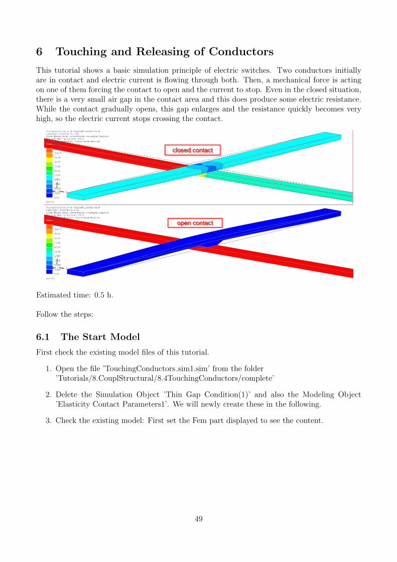
6 Touching and Releasing of Conductors
This tutorial shows a basic simulation principle of electric switches. Two conductors initiallyare in contact and electric current is flowing through both. Then, a mechanical force is actingon one of them forcing the contact to open and the current to stop. Even in the closed situation,there is a very small air gap in the contact area and this does produce some electric resistance.While the contact gradually opens, this gap enlarges and the resistance quickly becomes veryhigh, so the electric current stops crossing the contact.
Estimated time: 0.5 h.
Follow the steps:
6.1 The Start Model
First check the existing model files of this tutorial.
1. Open the file ’TouchingConductors sim1.sim’ from the folder’Tutorials/8.CouplStructural/8.4TouchingConductors/complete’
2. Delete the Simulation Object ’Thin Gap Condition(1)’ and also the Modeling Object’Elasticity Contact Parameters1’. We will newly create these in the following.
3. Check the existing model: First set the Fem part displayed to see the content.
49
• There are two conductor meshes and one air. Nothing is special. It is very similar tothe previous tutorials with electric conductors.
• One thing should be noticed: The Mesh Mating Condition between the two conductorsis also a usual condition of type ’Glue Coincident’. Until now the two conductors aretreated as if they were one. Later in the Sim file, we will define a ’Thin Gap Condition’with coupling to elasticity here. Thus, this face will become a contact that allows toopen.
4. Set the Sim part displayed and check the solution.
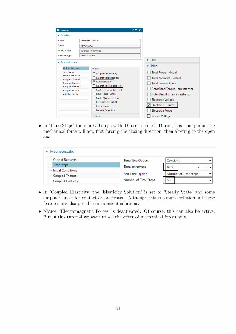
• Edit the existing solution ’MagStaDC ElasSta’ to check the settings. It is a magne-tostatic solution type with some basic output requests activated to check the current.
50
• in ’Time Steps’ there are 50 steps with 0.05 sec defined. During this time period themechanical force will act, first forcing the closing direction, then altering to the openone.
• In ’Coupled Elasticity’ the ’Elasticity Solution’ is set to ’Steady State’ and someoutput request for contact are activated. Although this is a static solution, all thesefeatures are also possible in transient solutions.
• Notice, ’Electromagnetic Forces’ is deactivated. Of course, this can also be active.But in this tutorial we want to see the effect of mechanical forces only.
51
5. Check the constraints.
• Like always in electromagnetics, there is a ’Flux Tangent’ condition at the outsidewalls of the meshed volumes.
• An elasticity constraint ’Elasticity(1)’ fixes all four electrode faces of the two conduc-tors.
6. Check the loads.
• There is a current load ’Current(1) Static’ applied to one of the electrode faces.This injects an electric current of 50000 amps into the conductor system. All threeremaining electrode faces have a voltage zero condition applied that allows the currentto enter or leave.
52
• A mechanical pressure load named ’Elasticity Load Ramp’ is of ’Analytic’ type anduses the following time dependent condition:($Time < 1)?(0.05 ∗ $Time) : (0.05− 0.05 ∗ ($Time− 1)).This form reads as: In case time is smaller 1, use the form 0.05 ∗ Time. In othercases, use the form 0.05− 0.05 ∗ (Time− 1). These are two linear functions, one forthe increase the other for the decrease of the mechanical pressure.
• Such were the existing features in the model. Nothing very new for the readers ofthis document. Following the new condition is created.
6.2 Creating a Thin Gap with EM-Elasticity Coupling
1. Create a new Simulation Object ’Thin Gap Condition’. Accept the default type ’Thin GapResistance’.
2. At ’Region’, select the contact face between the two conductors.
3. Set the ’Gap Thickness’ to 0.003 mm. This value represents the initial gap opening. Thereis already a small electric resistance because of this small gap.
4. Activate ’Effect on Electric Field’ and set the ’Electric Conductivity’ to the value 58 S/m.Notice, this is much less than copper with 58e6 S/m. Thus, as long as the gap remainssmall there is very small resistance.
5. Also activate ’Effect on Magnetic Field’.
6. Now activate ’Effect on Elasticity’ and create a ’Modeling Object’ for contact parameters(accept all defaults here).
7. Finally, activate ’Contact Distance affects Gap Thickness’. This leads to the desired effectof stopping the current when opening the contact.
53
6.3 Solving and Post Processing
1. Solve the solution. The 50 steps with contact need about 2 minutes solve time.
2. Display the Displacement results. Tip: For easier display, hide the Air mesh and also setthe edges to ’Feature’. In the below picture there are additionally the undeformed edgesshown. The left side shows the time of full force in contact direction. The right side showsthe time of full force in opposite. The gap arise can be clearly seen.
3. Set the result to ’Current Density’ now. Again, compare the two time steps as in picturebelow. Left side is the closed situation and the electric current being injected (top left)is split in three parts. Right side shows the open situation. The whole current now flowsthrough one conductor.
54
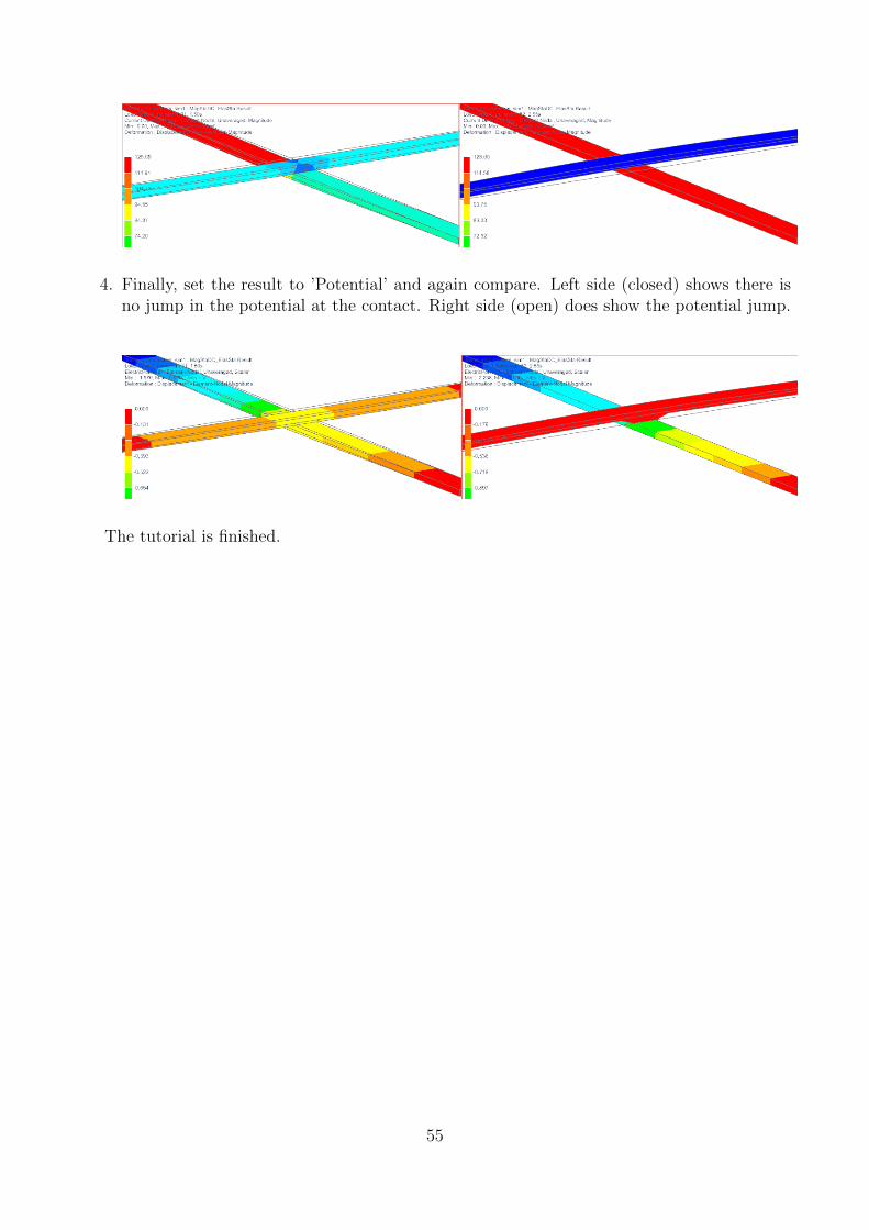
4. Finally, set the result to ’Potential’ and again compare. Left side (closed) shows there isno jump in the potential at the contact. Right side (open) does show the potential jump.
The tutorial is finished.
55
7 Electromechanical Switch
This tutorial shows a simple electro mechanical switch and its simulation principle. Three con-ductors are arranged as shown below (left) and loaded by three phase AC current. For simplicityin this tutorial, only one of the three has a switch. The switch is shown in detail below right.A free rotating joint connection without friction couples the switch to the conductor (top). Onthe other side (bottom) a clamped contact with friction connects to the other conductor side.In between there is a cylinder with mechanical pre-load, for instance by a screw. The pre-loadis given, also the friction coefficient and the electric currents.
Lorentz forces acting on the conductor system will maybe open up the switch and thereforethis simulation shall give an estimation about expected movements of the switch.
Estimated time: 1 h.
Features to learn:
• Elasticity Contact with effect on electric and magnetic field,
• Elasticity joint connections,
• Elasticity Bolt pre-load.
7.1 The Demo Model
First check the existing model files of this tutorial. This model is completely set up with allnecessary features. In the tutorial we walk through those features of interest and discuss them.Of course, a good idea for learning would be to start from the CAD model (in folder ’start’) andset up the whole model.
1. Open the file ’SimpleSwitch2 sim1.sim’ from the folder’Tutorials/8.CouplStructural/8.5SimpleSwitch/complete’
2. Check the existing model: First set the Fem part displayed to see the content.
56
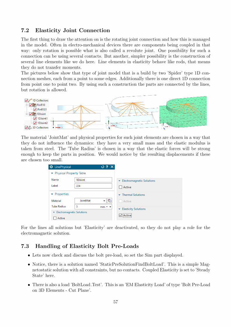
7.2 Elasticity Joint Connection
The first thing to draw the attention on is the rotating joint connection and how this is managedin the model. Often in electro-mechanical devices there are components being coupled in thatway: only rotation is possible what is also called a revolute joint. One possibility for such aconnection can be using several contacts. But another, simpler possibility is the construction ofseveral line elements like we do here. Line elements in elasticity behave like rods, that meansthey do not transfer moments.The pictures below show that type of joint model that is a build by two ’Spider’ type 1D con-nection meshes, each from a point to some edges. Additionally there is one direct 1D connectionfrom point one to point two. By using such a construction the parts are connected by the lines,but rotation is allowed.
The material ’JointMat’ and physical properties for such joint elements are chosen in a way thatthey do not influence the dynamics: they have a very small mass and the elastic modulus istaken from steel. The ’Tube Radius’ is chosen in a way that the elastic forces will be strongenough to keep the parts in position. We would notice by the resulting displacements if theseare chosen too small.
For the lines all solutions but ’Elasticity’ are deactivated, so they do not play a role for theelectromagnetic solution.
7.3 Handling of Elasticity Bolt Pre-Loads
• Lets now check and discuss the bolt pre-load, so set the Sim part displayed.
• Notice, there is a solution named ’StaticPreSolutionFindBoltLoad’. This is a simple Mag-netostatic solution with all constraints, but no contacts. Coupled Elasticity is set to ’SteadyState’ here.
• There is also a load ’BoltLoad Test’. This is an ’EM Elasticity Load’ of type ’Bolt Pre-Loadon 3D Elements - Cut Plane’.
57
As the names announce, we use a pre solution. The bolt load feature currently cannot directlyuse a force as input, instead it can use a given displacement (similar to negative strain) on thebolt. That enforced displacement or strain will result in force. Thus, the strategy is applying aninitial displacement, finding the resulting force and scaling the displacement to the desired boltforce. The corresponding displacement leading to that force will be the needed one for followingsimulations.
In this tutorial the desired bolt load is 5000 N. In the pre-solution we initially apply a dis-placement of -1 mm. Notice, the ’Ramp over Time Steps’ is zero. This option is useful only indynamic solutions, to prevent unwanted oscillations.
Thus, after solving, there results a deformed bolt and the tabular result shows the bolt force is8191.6 N (the plot below shows an over scaled deformation).
To find the necessary scaled displacement we divide the desired 5000 by 8191.6 what results ina scale of 0.6104. Thus, in the main solution ’SolutionSwitch’ we use -0.6104 mm as applieddisplacement. Also, in that dynamic solution, we use a ’Ramp over Time Steps’ set to 5 to avoidoscillations.
58
7.4 Contacts with EM Elasticity Coupling
Notice the Simulation Objects named ’Thin Gap CylPin’ and ’Thin Gap Out’. These definefaces at which electric current passes over a gap and that gap may change its thickness andsize depending on the elasticity solution. These contacts work as already demonstrated in theprevious tutorial ’8.4TouchingConductors’.
7.5 Additional Contacts to Avoid Penetration
Beside the contacts with EM Elasticity Coupling there are also some other contacts that simplyavoid penetration of the geometry while deforming. These are the Simulation Objects named’Side Contact’. They are of type ’Elasticity Contact’ and they work as already demonstrated inthe previous tutorial ’8.3ElasticityContact’.
7.6 Dynamic Solution for EM-Elasticity
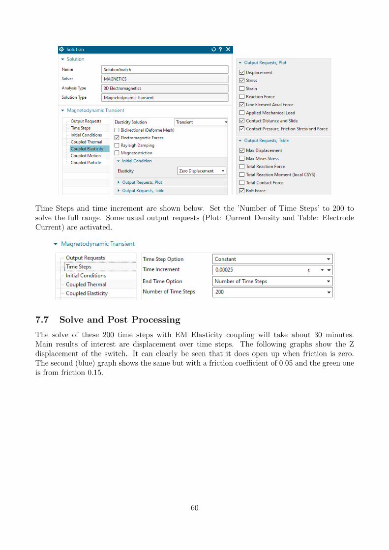
Finally, check solution ’SolutionSwitch’. There is nothing special in it. It is a Magnetodynamictransient one with Elasticity coupling also set to transient.
59
Time Steps and time increment are shown below. Set the ’Number of Time Steps’ to 200 tosolve the full range. Some usual output requests (Plot: Current Density and Table: ElectrodeCurrent) are activated.
7.7 Solve and Post Processing
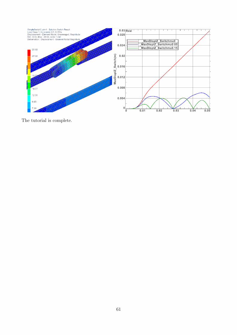
The solve of these 200 time steps with EM Elasticity coupling will take about 30 minutes.Main results of interest are displacement over time steps. The following graphs show the Zdisplacement of the switch. It can clearly be seen that it does open up when friction is zero.The second (blue) graph shows the same but with a friction coefficient of 0.05 and the green oneis from friction 0.15.