O-CNN: Octree-based Convolutional Neural Networks for 3D ShapeAnalysis
PENG-SHUAI WANG, Tsinghua University and Microsoft Research AsiaYANG LIU, Microsoft Research AsiaYU-XIAO GUO, University of Electronic Science and Technology of China and Microsoft Research AsiaCHUN-YU SUN, Tsinghua University and Microsoft Research AsiaXIN TONG, Microsoft Research Asia
normal field
octree input (d-depth)
...
convolution pooling convolution pooling
d d-1 3 2
...
... ...
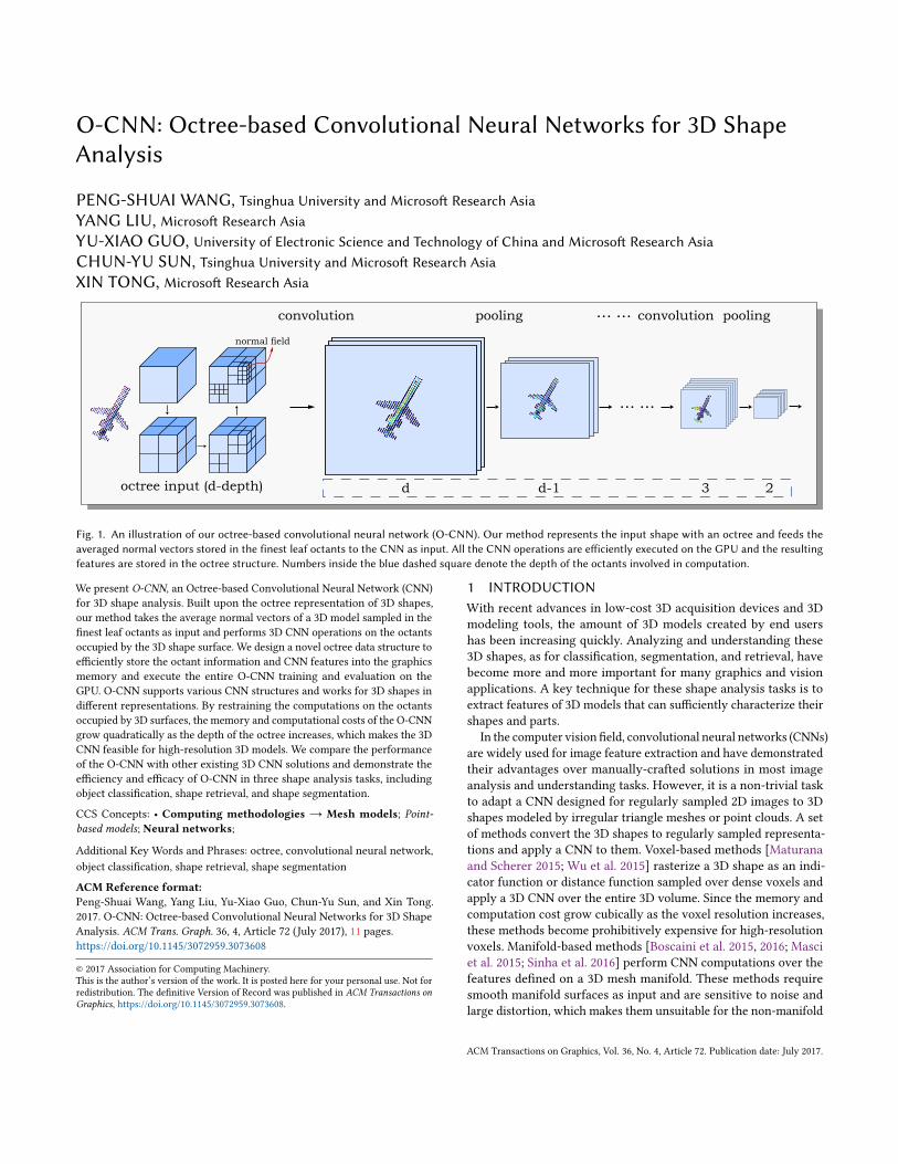
Fig. 1. An illustration of our octree-based convolutional neural network (O-CNN). Our method represents the input shape with an octree and feeds theaveraged normal vectors stored in the finest leaf octants to the CNN as input. All the CNN operations are efficiently executed on the GPU and the resultingfeatures are stored in the octree structure. Numbers inside the blue dashed square denote the depth of the octants involved in computation.
We present O-CNN, an Octree-based Convolutional Neural Network (CNN)for 3D shape analysis. Built upon the octree representation of 3D shapes,our method takes the average normal vectors of a 3D model sampled in thefinest leaf octants as input and performs 3D CNN operations on the octantsoccupied by the 3D shape surface. We design a novel octree data structure toefficiently store the octant information and CNN features into the graphicsmemory and execute the entire O-CNN training and evaluation on theGPU. O-CNN supports various CNN structures and works for 3D shapes indifferent representations. By restraining the computations on the octantsoccupied by 3D surfaces, the memory and computational costs of the O-CNNgrow quadratically as the depth of the octree increases, which makes the 3DCNN feasible for high-resolution 3D models. We compare the performanceof the O-CNN with other existing 3D CNN solutions and demonstrate theefficiency and efficacy of O-CNN in three shape analysis tasks, includingobject classification, shape retrieval, and shape segmentation.
1 INTRODUCTIONWith recent advances in low-cost 3D acquisition devices and 3Dmodeling tools, the amount of 3D models created by end usershas been increasing quickly. Analyzing and understanding these3D shapes, as for classification, segmentation, and retrieval, havebecome more and more important for many graphics and visionapplications. A key technique for these shape analysis tasks is toextract features of 3D models that can sufficiently characterize theirshapes and parts.
In the computer vision field, convolutional neural networks (CNNs)are widely used for image feature extraction and have demonstratedtheir advantages over manually-crafted solutions in most imageanalysis and understanding tasks. However, it is a non-trivial taskto adapt a CNN designed for regularly sampled 2D images to 3Dshapes modeled by irregular triangle meshes or point clouds. A setof methods convert the 3D shapes to regularly sampled representa-tions and apply a CNN to them. Voxel-based methods [Maturanaand Scherer 2015; Wu et al. 2015] rasterize a 3D shape as an indi-cator function or distance function sampled over dense voxels andapply a 3D CNN over the entire 3D volume. Since the memory andcomputation cost grow cubically as the voxel resolution increases,these methods become prohibitively expensive for high-resolutionvoxels. Manifold-based methods [Boscaini et al. 2015, 2016; Masciet al. 2015; Sinha et al. 2016] perform CNN computations over thefeatures defined on a 3D mesh manifold. These methods requiresmooth manifold surfaces as input and are sensitive to noise andlarge distortion, which makes them unsuitable for the non-manifold
ACM Transactions on Graphics, Vol. 36, No. 4, Article 72. Publication date: July 2017.
72:2 • Peng-Shuai Wang, Yang Liu, Yu-Xiao Guo, Chun-Yu Sun, and Xin Tong
3D models in many 3D shape repositories. Multiple-view based ap-proaches [Bai et al. 2016; Shi et al. 2015; Su et al. 2015] render the3D shape into a set of 2D images observed from different views andfeed the stacked images to the CNN. However, it is unclear howto determine the view positions to cover full 3D shapes and avoidself-occlusions.
We present an octree-based convolutional neural network, namedO-CNN, for 3D shape analysis. The key idea of our method is to rep-resent the 3D shapes with octrees and perform 3D CNN operationsonly on the sparse octants occupied by the boundary surfaces of 3Dshapes. To this end, the O-CNN takes the average normal vectors ofa 3D model sampled in the finest leaf octants as input and computesfeatures for the finest level octants. After pooling, the features aredown-sampled to the parent octants in the next coarser level andare fed into the next O-CNN layer. This process is repeated until allO-CNN layers are evaluated.The main technical challenge of the O-CNN is to parallelize the
O-CNN computations defined on the sparse octants so that theycan be efficiently executed on the GPU. To this end, we designa novel octree structure that stores the features and associatedoctant information into the graphics memory for supporting allCNN operations on the GPU. In particular, we pack the features anddata of sparse octants at each depth as continuous arrays. A labelbuffer is introduced to find the correspondence between the featuresat different levels for efficient convolution and pooling operations.To efficiently compute 3D convolutions with an arbitrary kernel size,we build a hash table to quickly construct the local neighborhoodvolume of eight sibling octants and compute the 3D convolutions ofthese octants in parallel. With the help of this octree structure, theentire training and evaluation process can be efficiently executedon the GPU.
The O-CNN provides a generic and efficient CNN solution for 3Dshape analysis. It supports various CNN structures and works for3D shapes in different representations. By restraining the CNN com-putations and features on sparse octants of the 3D shape boundaries,the memory and computation costs of O-CNN grow quadraticallyas the octree depth increases, which makes it efficient for analyzinghigh-resolution 3D models. To demonstrate the efficiency of theO-CNN, we construct an O-CNN with basic CNN layers as shownin Figure 1. We train this O-CNN model with 3D shape datasetsand refine the O-CNN models with different back-ends for threeshape analysis tasks, including object classification, shape retrieval,and shape segmentation. Compared to existing 3D CNN solutions,our method achieves comparable or better accuracy with much lesscomputational and memory costs in all three shape analysis tasks.We also evaluate the performance of the O-CNN with different oc-tree depths in object classification and demonstrate the efficiencyand efficacy of the O-CNN for analyzing high-resolution 3D shapes.
2 RELATED WORKIn this section, we first review existing CNN approaches and otherdeep learning methods for 3D shape analysis. Then we discuss theGPU based octree structures used in different graphics applications.
CNNs for 3D shape analysis. A set of CNN methods have beenpresented for 3D shape analysis. We classify these approaches into
several classes according to the 3D shape representation used ineach solution.
Voxel-based methods. model the 3D shape as a function sampledon voxels and define a 3D CNN over voxels for shape analysis. Wu etal. [2015] proposed 3D ShapeNets for object recognition and shapecompletion. Maturana and Scherer [2015] improve 3D ShapeNetswith fewer input parameters defined in each voxel. These full-voxel-based methods are limited to low resolutions like 303 due to thehigh memory and computational cost.To reduce the computational cost of full-voxel based methods,
Graham [2015] proposes the 3D sparse CNNs that apply CNN opera-tions to active voxels and activate only the neighboring voxels insidethe convolution kernel. However, the method quickly becomes lessefficient as the number of convolution layers between the poolinglayers increases. For a CNN with deep layers and a large kernelsize, the computational and memory cost of this method is stillhigh. Riegler et al. [2017] combine the octree and a grid structureto support high-resolution 3D CNNs. Their method limits the 3DCNN to the interior volume of 3D shapes and becomes less efficientthan the full-voxel-based solution when the volume resolution islower than 643. Our method limits the 3D CNN to the octants ofthe 3D shape boundaries and leverages a novel octree structure forefficiently training and evaluating the O-CNN on the GPU.
Manifold-based methods. perform CNN operations over the geo-metric features defined on a 3D mesh manifold. Some methodsparameterize the 3D surfaces to 2D patches [Boscaini et al. 2015,2016; Masci et al. 2015; Sinha et al. 2016] or geometry images andfeed the regularly sampled feature images into a 2D CNN for shapeanalysis. Other methods extend the CNN to the graphs defined byirregular triangle meshes [Bronstein et al. 2017]. Although thesemethods are robust to isometric deformation of 3D shapes, they areconstrained to smooth manifold meshes. The local features usedin these methods are always computationally expensive. A goodsurvey of these techniques can be found in [Bronstein et al. 2017].
Multiview-based methods. represent the 3D shape with a set of im-ages rendered from different views and take the image stacks as theinput of a 2DCNN for shape analysis [Bai et al. 2016; Qi et al. 2016; Suet al. 2015]. Although these methods can directly exploit the image-based CNNs for 3D shape analysis and handle high-resolution inputs,it is unclear how to determine the number of views and distributethe views to cover the 3D shape while avoiding self-occlusions. Ourmethod is based on the octree representation and avoids the viewselection issue. It can also handle high-resolution inputs and achievesimilar performance and accuracy to multiview-based methods.
Deep learning for 3D shape analysis. Besides the CNN, other deeplearning methods have also been proposed for 3D shape analysis.For shape segmentation, Guo et al. [2015] extract low-level featurevectors on each facet and pack them as images for training. Liet al. [2016] introduce a probing filter that can efficiently extractfeatures and work for a higher resolution like 643. However, thisapproach cannot extract fine structures of shapes; therefore, it is notsuitable for tasks like shape segmentation. Qi et al. [2017] propose aneural network based on an unordered point cloud that can achievegood performance on shape classification and segmentation.
ACM Transactions on Graphics, Vol. 36, No. 4, Article 72. Publication date: July 2017.
O-CNN: Octree-based Convolutional Neural Networks for 3D Shape Analysis • 72:3
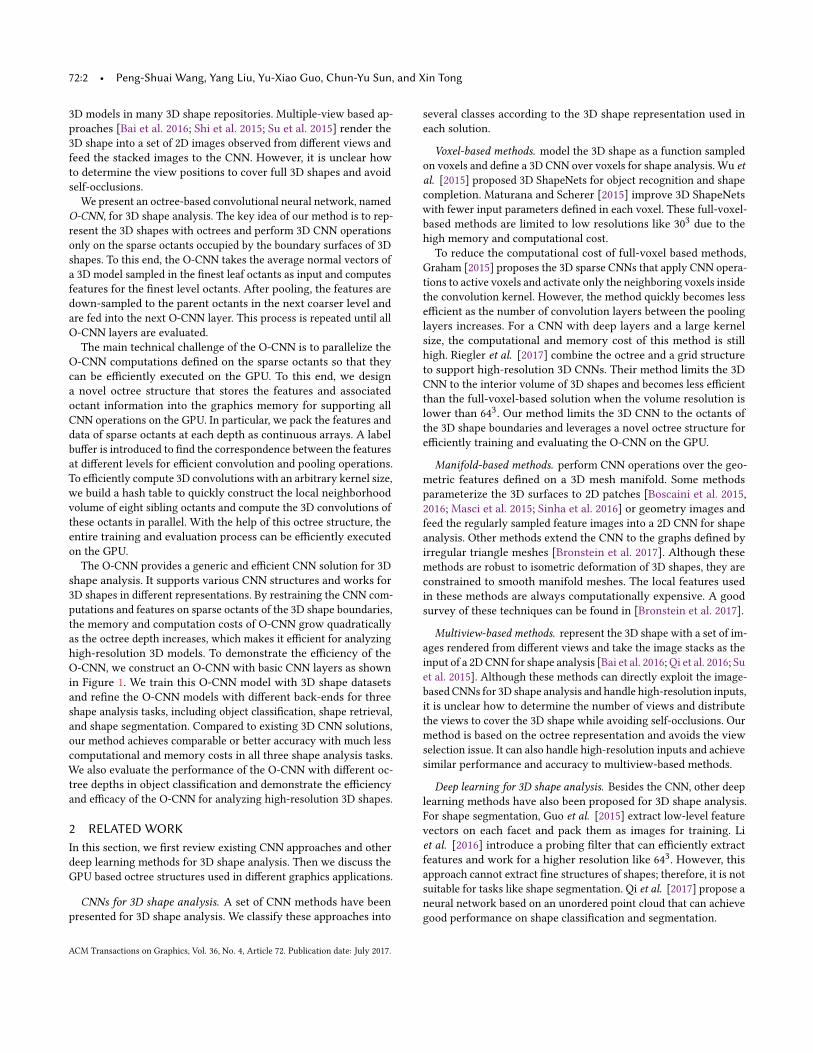
Fig. 2. A 2D quadtree illustration of our octree structure. (a) Given an input 2D shape marked in red, we construct a 2-depth quadtree. The squares that arenot occupied by the shape are empty nodes. The numbers inside quad nodes are their shuffled keys. (b) The shuffle key vectors Sl , l = 0 . . . 2, , each of whichstores the shuffled keys of the quad nodes at the l -th depth. (c) The label vectors Ll , l = 0 . . . 2, each of which stores the labels of the quad nodes at the l -thdepth. For empty nodes, their labels are set to zero. For non-empty nodes, the label p of a node indicates it is the p-th non-empty node at this depth. The labelbuffer is used to find the correspondence from the parent node to its child nodes. (d) The results of CNN convolutions over the input signal are stored in afeature map T2. When T2 is down-sampled by a CNN operation, such as pooling, the downsampled results are assigned to the first, the second and the thirdentries of T1. The label vector L1 at the first depth is used to find the correspondence between the nodes at two depths.
GPU-based octree structures. The octree structure [Meagher 1982]is widely used in computer graphics for various tasks including ren-dering, modeling and collision detection. Zhou et al. [2011] proposea GPU-based octree construction method and use the constructedoctree for reconstructing surfaces on the GPU. Different from theoctree structure that is optimized for surface reconstruction, theoctree structure designed in our method is optimized for CNN train-ing and evaluation. For this purpose, we discard the pointers fromparent octants to children octants and introduce a label array forfinding correspondence of octants at different depths for downsam-pling. Instead of computing the neighborhood of a single octant, weconstruct the neighborhoods for eight children nodes of a parentnode for fast convolution computation.
3 3D CNNS ON OCTREE BASED 3D SHAPESGiven an oriented 3D model (e.g. an oriented triangle mesh or apoint cloud with oriented normals), our method first constructs theoctree of the input 3D model and packs the information needed forCNN operations in the octree (Section 3.1). With the help of thisoctree structure, all the CNN operations can be efficiently executedon the GPU (Section 3.2).
3.1 Octree for 3D CNNsOctree construction. To construct an octree for an input 3D model,
we first uniformly scale the 3D shape into an axis-aligned unit 3Dbounding cube and then recursively subdivide the bounding cubeof the 3D shape in breadth-first order. In each step, we traverseall non-empty octants occupied by the 3D shape boundary at thecurrent depth l and subdivide each of them to eight child octants atthe next depth l + 1. We repeat this process until the pre-definedoctree depth d is reached. Figure 2(a) illustrates a 2-depth quadtreeconstructed for a 2D shape (marked in red).After the octree is constructed, we collect a set of properties re-
quired for CNN operations at each octant and store their values inthe octree. Specifically, we compute a shuffle key [Wilhelms and
Van Gelder 1992] and a label for each octant in the octree. Mean-while, our method extracts the input signal of the CNN from the3D shape stored in the finest leaf nodes and records the resultingCNN features at each octant. As shown in Figure 2, we organize thedata stored in the octree in a depth order. At each depth, we sort theoctants according to the ascending order of their shuffle keys andpack their property values into a set of 1D property vectors. All theproperty vectors share the same index, and the length of the vectorsis the number of octants at the current depth. In the following, wedescribe the definition and implementation details of each propertydefined in our octree structure.
Shuffle key. The shuffle key of an octant O at depth l encodesits position in 3D space with an unique 3 l-bit string key(O) :=x1y1z1x2y2z2 . . . xlylzl [Wilhelms and Van Gelder 1992], whereeach three-bit group xi ,yi , zi ∈ {0, 1} defines its relative posi-tion in the 3D cube of its parent octant. The integer coordinates(x ,y, z) of an octant O are determined by x = (x1x2 . . . xl ),y =(y1y2 . . .yl ), z = (z1z2 . . . zl ). We sort all the octants by their shuf-fle keys according to the ascending order and store the sorted shufflekeys of all octants at the l-th depth in a shuffle key vector Sl , whichis used later for constructing the neighborhood of an octant for 3Dconvolution. In our implementation, each shuffle key is stored in a32 bit integer. Figure 2(a) illustrates the shuffle keys of all quadtreenodes and Figure 2(b) demonstrates the corresponding shuffle keyarray at each depth.
Label. In CNN computations, the pooling operation is frequentlyused to downsample the features computed at the l-th depth octantsto their parent octants at the (l − 1)-th depth. As a result, we needto quickly find the parent-child relationship of the octants at theadjacent depths. To this end, we assign a label p for a non-emptyoctant at the l-th depth, which indicates that it is thep-th non-emptyoctant in the sorted octant list of the l-th depth. For empty octants,we simply set its label as zero. The labels of all octants at the l-thdepth are stored in a label vector Ll . Figure 2(c) illustrates the labelvector for each depth of a quadtree. For the non-empty quad node
ACM Transactions on Graphics, Vol. 36, No. 4, Article 72. Publication date: July 2017.
72:4 • Peng-Shuai Wang, Yang Liu, Yu-Xiao Guo, Chun-Yu Sun, and Xin Tong
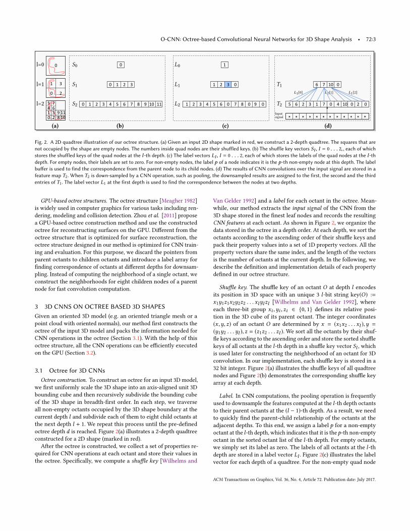
Fig. 3. Left: the original 3D shape. Middle: the voxelized 3D shape. Right:the octree representation with normals sampled at the finest leaf octants.
marked in blue, its label is 3 (L1[2] = 3) because it is the third non-empty node at the first depth, while the node with the shuffle key 0is the first one and the node with the shuffle key 1 is the second one.
Given a non-empty node with index j at the l-th depth, we com-pute the index k of its first child octant at the (l + 1)-th depth byk = 8 × (Ll [j] − 1). This is based on two observations. First, onlythe non-empty octants at the l-th depth are subdivided. Second,since we sort the octants according to the ascending order of theirshuffle keys, the eight children of an octant are sequentially stored.Moreover, the child octants and their non-empty parents follow thesame order in their own property vectors. As shown in Figure 2(c),the last four nodes at the second depth are created by the thirdnon-empty node at the first depth (marked in blue).
Input signal. We use the averaged normal vectors computed atthe finest leaf octants as the input signal of the CNN. For emptyleaf octants, we simply assign a zero vector as the input signal. Fornon-empty leaf octants, we sample the 3D shape surface embeddedin the leaf octant with a set of points and average the normals of allsampled points as the input signal at this leaf octant. We store theinput signals of all leaf octants into an input signal vector. The sizeof the vector is the number of the finest leaf octants in the octree.Compared to the binary indicator function used in many voxel-
based CNN methods [Maturana and Scherer 2015; Wu et al. 2015],the normal signal is very sparse, i.e. only non-zero on the surface,and the averaged normals sampled in the finest leaf octants betterrepresent the orientation of the local 3D shapes and provide morefaithful 3D shape information to the CNN. Figure 3 compares avoxelized 3D model and an octree representation of the same 3Dshape rendered by oriented disks sampled at leaf octants, where thesize of the leaf octant is the same as the voxel size. As shown inthe figure, the octree representation (on the right) is more faithfulto the ground truth 3D shape (on the left) than the voxel basedrepresentation (in the middle).
CNN features. For each 3D convolution kernel defined at the l-thdepth, we record the convolution results on all the octants at thel-th depth in a feature map vector Tl .
Mini-batch of 3D models. For 3D objects in a mini-batch used inthe CNN training, their octrees are not the same. To support efficientCNN training on the GPU, we merge these octrees into one super-octree. For each octree depth l , we concatenate the property vectors(Sl , Ll and Tl ) of all 3D objects to S∗l , L
∗l and T
∗l of the super-octree.
After that, we update the shuffle keys in S∗l by using the highest 8bits of each shuffle key to store the object index. We also updatethe label vector L∗l in the super-octree to represent the index ofeach non-empty octant in the whole super-octree. After that, thesuper-octree can be directly used in the CNN training.
3.2 CNN operations on the OctreeThe most common operations in a CNN are convolution, pooling,and the inverse deconvolution and unpooling. With the help of ouroctree data structure, all these CNN operations can be efficientlyimplemented on the GPU.
3D Convolution. For applying the convolution operator to an oc-tant, one needs to pick its neighboring octants at the same octreedepth. To compute the convolution efficiently, we write the convo-lution operator Φc in the unrolled form:
Φc(O) =∑n
∑i
∑j
∑k
W(n)i jk ·T (n)(Oi jk ).
Here Oi jk represents a neighboring octant of O and T (·) representsthe feature vector associated with Oi jk . And T (n)(·) represents then-th channel of the feature vector, andW (n)
i jk are the weights of theconvolution operation. If Oi jk does not exist in the octree, T (Oi jk )
is set to the zero vector. In this form, the convolution operation canbe converted to a matrix product [Chellapilla et al. 2006; Jia et al.2014] and computed efficiently on the GPU.
The convolution operator with kernel size K requires the accessof K3 − 1 neighboring octants of an octant. A possible solution is topre-compute and store neighboring information. However, a CNNis normally trained on a batch of shapes. When K is very large,this will cause a significant amount of I/O processing and a largememory footprint. We build a hash table:H : key(O) 7→ index(O)to facilitate the search, where index(O) records the position of O inS . Because the amortized time complexity of a hash table is constant,this choice can be regarded as a balance of computation cost andmemory cost for the CNN. Given the shuffled key stored in the vectorSl , the integer coordinates (x ,y, z) of the octant can be restored, thenthe coordinates of the neighboring octants can be computed easilyin constant time, as can their corresponding shuffled keys. Giventhe shuffled keys of neighboring octants, the hash table is efficientlysearched in parallel to get their indices, according to which theneighboring data information is gathered and then the convolutionoperation can be applied.If the stride of convolution is 1, the above operation is applied
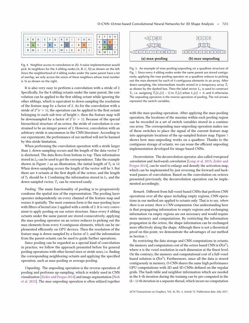
to all existing octants at the current octree depth. Naïvely, for eachoctant the hash table will be searched K3 − 1 times. However, theneighborhood of eight sibling octants under the same parent have alot of overlap, and there are only (K+1)3 individual octants includingthe eight octants. The neighborhood search can be further sped upby just searching the (K + 1)3 − 8 neighboring octants for each ofthe eight sibling octants. Concretely, if the kernel size is 3, then thisoptimization can accelerate the neighboring search operation bymore than 2 times. Figure 4 illustrates this efficient neighborhoodsearch on a 2D quadtree.
ACM Transactions on Graphics, Vol. 36, No. 4, Article 72. Publication date: July 2017.
O-CNN: Octree-based Convolutional Neural Networks for 3D Shape Analysis • 72:5
M
A
B
C
D
E F G H
N
P
K
O
L
J
I
M
A
B
C
D
N
P
O
L M
A
B
C
D
KL
J
I
A
B
C
D
E F G
P
O A
B
C
D
F G H
J
I
Fig. 4. Neighbor access in convolution in 2D. A naïve implementation wouldpick 36 neighbors for the 4 sibling nodes (A, B, C, D) as shown on the left.Since the neighborhood of 4 sibling nodes under the same parent have a lotof overlap, we only access the union of these neighbors whose total numberis 16 as shown on the right.
It is also very easy to perform a convolution with a stride of 2.Specifically, for the 8 sibling octants under the same parent, the con-volution can be applied to the first sibling octant while ignoring theother siblings, which is equivalent to down-sampling the resolutionof the feature map by a factor of 2. As for the convolution with astride of 2r (r > 1), the operation can be applied to the first octantbelonging to each sub-tree of height r , then the feature map willbe downsampled by a factor of 2r (r > 1). Because of the specialhierarchical structure of an octree, the stride of convolution is con-strained to be an integer power of 2. However, convolution with anarbitrary stride is uncommon in the CNN literature. According toour experiments, the performance of our method will not be harmedby this stride limitation.
When performing the convolution operation with a stride largerthan 1, down-sampling occurs and the length of the data vector Tis shortened. The data flows from bottom to top. Then informationstored in Ll can be used to get the correspondence. Take the exampleshown in Figure 2 as an illustration, the initial length of T2 is 12.When down-sampling occurs the length of the vector will be 3. Butthere are 4 octants at the first depth of the octree, and the lengthof T1 should be 4. Combining the information stored in L1 and thedown-sampled vector, T1 can be renewed easily.
Pooling. The main functionality of pooling is to progressivelycondense the spatial size of the representation. The pooling layeroperates independently on every channel of the feature map andresizes it spatially. The most common form is the max-pooling layerwith filters of kernel size 2 applied with a stride of 2. It is very conve-nient to apply pooling on our octree structure. Since every 8 siblingoctants under the same parent are stored consecutively, applyingthe max-pooling operator on an octree reduces to picking out themax elements from every 8 contiguous elements, which can be im-plemented efficiently on GPU devices. Then the resolution of thefeature map is down-sampled by a factor of 2, and the informationfrom the parent octants can be used to guide further operations.Since pooling can be regarded as a special kind of convolution
in practice, we follow the approach presented before for generalpooling operations with other kernel sizes or stride sizes, i.e. findingthe corresponding neighboring octants and applying the specifiedoperation, such as max-pooling or average-pooling.
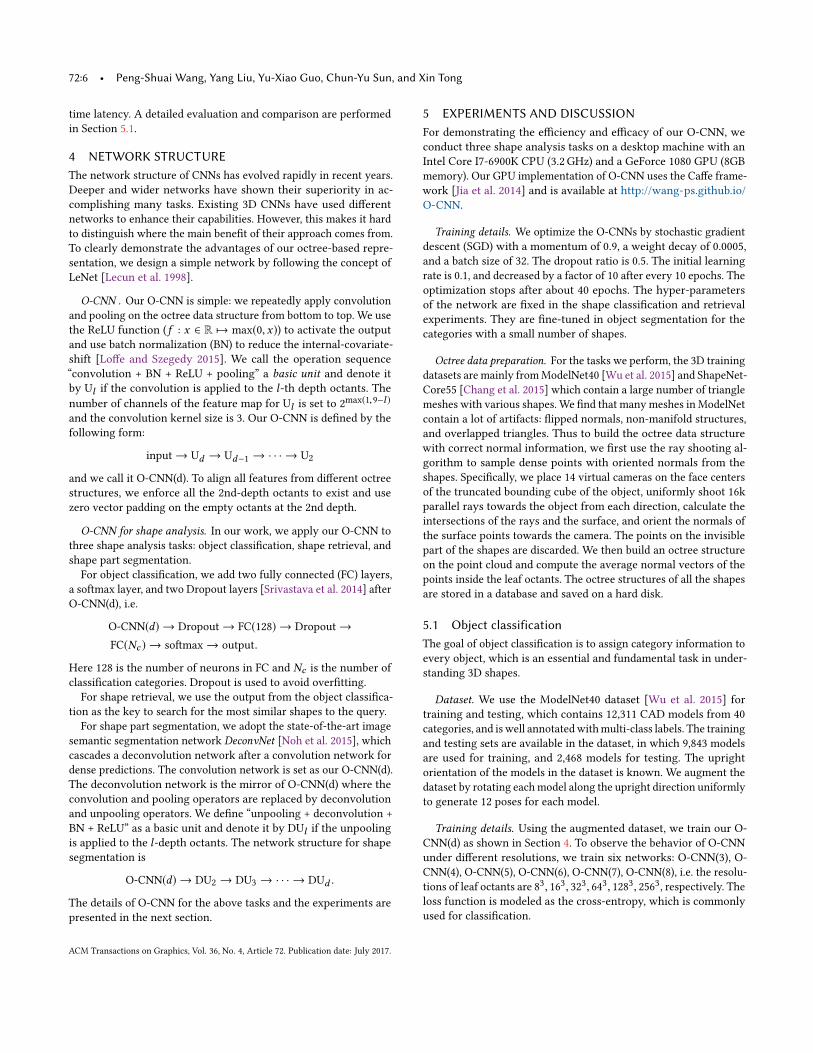
Unpooling. The unpooling operation is the reverse operation ofpooling and performs up-sampling, which is widely used in CNNvisualization [Zeiler and Fergus 2014] and image segmentation [Nohet al. 2015]. The max-unpooling operation is often utilized together
7 106
104 071 0 2 06 2 35
7 10 06
2 38
30 020 0 0 08 0 00
2 3 08
(a) max-pooling (b) max-unpooling
T1
T̂1
T2
Fig. 5. An example of max-pooling/unpooling on a quadtree structure ofFig. 2. Since every 4 sibling nodes under the same parent are stored contigu-ously, applying the max-pooling operator on a quadtree reduces to pickingout the max element for each of 4 contiguous elements in an array. Afterdown-sampling, the intermediate results stored in a temporary array T̂1as shown by the dashed box. Then the label vector L1 is used to constructT1, i.e. assigning T̂1[L1[i] − 1] to T1[i] when L1[i] > 0, and 0 otherwise.The unpooling operation is the reverse operation of pooling. The red arrowsrepresent the switch variables.
with the max-pooling operation. After applying the max-poolingoperation, the locations of the maxima within each pooling regioncan be recorded in a set of switch variables stored in a continu-ous array. The corresponding max-unpooling operation makes useof these switches to place the signal of the current feature mapinto appropriate locations of the up-sampled feature map. Figure 5shows how max-unpooling works on a quadtree. Thanks to thecontiguous storage of octants, we can reuse the efficient unpoolingimplementation developed for image-based CNNs.
Deconvolution. The deconvolution operator, also called transposedconvolution and backwards convolution [Long et al. 2015; Zeiler andFergus 2014], can be used to enlarge and densify the activation map,which can be implemented by just reversing the forward and back-ward passes of convolution. Based on the convolution on octreespresented previously, the deconvolution operation can be imple-mented accordingly.
Remark. Different from full-voxel-based CNNs that perform CNNoperations over all the space including empty regions, CNN opera-tions in our method are applied to octants only. That is to say, wherethere is an octant, there is CNN computation. Our understanding hereis that propagating information to empty regions and exchanginginformation via empty regions are not necessary and would requiremore memory and computations. By restricting the informationpropagation in the octree, the shape information can be exchangedmore effectively along the shape. Although there is not a theoreticalproof on this point, we demonstrate the advantages of our methodin Section 5.
By restricting the data storage and CNN computations in octants,the memory and computation cost of the octree based CNN is O(n2),where n is the voxel resolution in each dimension at the finest level.On the contrary, the memory and computational cost of a full-voxelbased solution is O(n3). Furthermore, since all the data is storedcontiguously in memory, O-CNN shares the same high performanceGPU computations with 2D and 3D CNNs defined on the regulargrids. The hash table and neighbor information which are neededin the k-th iteration during the training can be pre-computed in the(k−1)-th iteration in a separate thread, which incurs no computation
ACM Transactions on Graphics, Vol. 36, No. 4, Article 72. Publication date: July 2017.
72:6 • Peng-Shuai Wang, Yang Liu, Yu-Xiao Guo, Chun-Yu Sun, and Xin Tong
time latency. A detailed evaluation and comparison are performedin Section 5.1.
4 NETWORK STRUCTUREThe network structure of CNNs has evolved rapidly in recent years.Deeper and wider networks have shown their superiority in ac-complishing many tasks. Existing 3D CNNs have used differentnetworks to enhance their capabilities. However, this makes it hardto distinguish where the main benefit of their approach comes from.To clearly demonstrate the advantages of our octree-based repre-sentation, we design a simple network by following the concept ofLeNet [Lecun et al. 1998].
O-CNN . Our O-CNN is simple: we repeatedly apply convolutionand pooling on the octree data structure from bottom to top. We usethe ReLU function (f : x ∈ R 7→ max(0,x)) to activate the outputand use batch normalization (BN) to reduce the internal-covariate-shift [Loffe and Szegedy 2015]. We call the operation sequence“convolution + BN + ReLU + pooling” a basic unit and denote itby Ul if the convolution is applied to the l-th depth octants. Thenumber of channels of the feature map for Ul is set to 2max(1,9−l )
and the convolution kernel size is 3. Our O-CNN is defined by thefollowing form:
input → Ud → Ud−1 → · · · → U2
and we call it O-CNN(d). To align all features from different octreestructures, we enforce all the 2nd-depth octants to exist and usezero vector padding on the empty octants at the 2nd depth.
O-CNN for shape analysis. In our work, we apply our O-CNN tothree shape analysis tasks: object classification, shape retrieval, andshape part segmentation.
For object classification, we add two fully connected (FC) layers,a softmax layer, and two Dropout layers [Srivastava et al. 2014] afterO-CNN(d), i.e.
Here 128 is the number of neurons in FC and Nc is the number ofclassification categories. Dropout is used to avoid overfitting.For shape retrieval, we use the output from the object classifica-
tion as the key to search for the most similar shapes to the query.For shape part segmentation, we adopt the state-of-the-art image
semantic segmentation network DeconvNet [Noh et al. 2015], whichcascades a deconvolution network after a convolution network fordense predictions. The convolution network is set as our O-CNN(d).The deconvolution network is the mirror of O-CNN(d) where theconvolution and pooling operators are replaced by deconvolutionand unpooling operators. We define “unpooling + deconvolution +BN + ReLU” as a basic unit and denote it by DUl if the unpoolingis applied to the l-depth octants. The network structure for shapesegmentation is
O-CNN(d) → DU2 → DU3 → · · · → DUd .
The details of O-CNN for the above tasks and the experiments arepresented in the next section.
5 EXPERIMENTS AND DISCUSSIONFor demonstrating the efficiency and efficacy of our O-CNN, weconduct three shape analysis tasks on a desktop machine with anIntel Core I7-6900K CPU (3.2 GHz) and a GeForce 1080 GPU (8GBmemory). Our GPU implementation of O-CNN uses the Caffe frame-work [Jia et al. 2014] and is available at http://wang-ps.github.io/O-CNN.
Training details. We optimize the O-CNNs by stochastic gradientdescent (SGD) with a momentum of 0.9, a weight decay of 0.0005,and a batch size of 32. The dropout ratio is 0.5. The initial learningrate is 0.1, and decreased by a factor of 10 after every 10 epochs. Theoptimization stops after about 40 epochs. The hyper-parametersof the network are fixed in the shape classification and retrievalexperiments. They are fine-tuned in object segmentation for thecategories with a small number of shapes.
Octree data preparation. For the tasks we perform, the 3D trainingdatasets are mainly fromModelNet40 [Wu et al. 2015] and ShapeNet-Core55 [Chang et al. 2015] which contain a large number of trianglemeshes with various shapes. We find that many meshes in ModelNetcontain a lot of artifacts: flipped normals, non-manifold structures,and overlapped triangles. Thus to build the octree data structurewith correct normal information, we first use the ray shooting al-gorithm to sample dense points with oriented normals from theshapes. Specifically, we place 14 virtual cameras on the face centersof the truncated bounding cube of the object, uniformly shoot 16kparallel rays towards the object from each direction, calculate theintersections of the rays and the surface, and orient the normals ofthe surface points towards the camera. The points on the invisiblepart of the shapes are discarded. We then build an octree structureon the point cloud and compute the average normal vectors of thepoints inside the leaf octants. The octree structures of all the shapesare stored in a database and saved on a hard disk.
5.1 Object classificationThe goal of object classification is to assign category information toevery object, which is an essential and fundamental task in under-standing 3D shapes.
Dataset. We use the ModelNet40 dataset [Wu et al. 2015] fortraining and testing, which contains 12,311 CAD models from 40categories, and is well annotatedwithmulti-class labels. The trainingand testing sets are available in the dataset, in which 9,843 modelsare used for training, and 2,468 models for testing. The uprightorientation of the models in the dataset is known. We augment thedataset by rotating eachmodel along the upright direction uniformlyto generate 12 poses for each model.
Training details. Using the augmented dataset, we train our O-CNN(d) as shown in Section 4. To observe the behavior of O-CNNunder different resolutions, we train six networks: O-CNN(3), O-CNN(4), O-CNN(5), O-CNN(6), O-CNN(7), O-CNN(8), i.e. the resolu-tions of leaf octants are 83, 163, 323, 643, 1283, 2563, respectively. Theloss function is modeled as the cross-entropy, which is commonlyused for classification.
ACM Transactions on Graphics, Vol. 36, No. 4, Article 72. Publication date: July 2017.
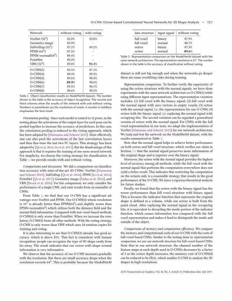
Table 1. Object classification results on ModelNet40 dataset. The numbershown in the table is the accuracy of object recognition. The second andthird columns show the results of the network with and without voting.Numbers in parentheses are the resolutions of voxels. A number in boldfaceemphasizes the best result.
Orientation pooling. Since each model is rotated to 12 poses, in thetesting phase the activations of the output layer for each pose can bepooled together to increase the accuracy of predictions. In this case,the orientation pooling is reduced to the voting approach, whichhas been adopted by [Maturana and Scherer 2015]. More effectively,one can also pool the activations of the last convolution layersand then fine-tune the last two FC layers. This strategy has beenadopted by [Qi et al. 2016; Su et al. 2015]. But the disadvantage of thisapproach is that it requires the training of one more neural network.For simplicity, we choose the voting strategy for classification. InTable 1, we provide results with and without voting.
Comparisons and discussion. We did a comparison on classifica-tion accuracy with state-of-the-art 3D CNNs: VoxNet [Maturanaand Scherer 2015], SubVolSup [Qi et al. 2016], FPNN [Li et al. 2016],PointNet [Qi et al. 2017], Geometry image [Sinha et al. 2016], andVRN [Brock et al. 2016]. For fair comparison, we only consider theperformance of a single CNN, and omit results from an ensemble ofCNNs.From Table 1, we find that our O-CNN has a significant ad-
vantage over VoxNet and FPNN. Our O-CNN(4) whose resolutionis 163 is already better than FPNN(643) and slightly worse thanFPNN+normal(643) which utilizes both the distance field and thenormal field information. Compared with non voxel-based methods,O-CNN(4) is only worse than PointNet. When we increase the reso-lution, O-CNN(5) beats all other methods. With the voting strategy,O-CNN is only worse than VRN which uses 24 rotation copies fortraining and voting.It is also interesting to see that O-CNN(3) already has good ac-
curacy, which is above 85%. This fact is consistent with humanrecognition: people can recognize the type of 3D shape easily fromfar away. The result indicates that our octree with shape normalinformation is very informative.
We observe that the accuracy of our O-CNN increases graduallywith the resolution. But there are small accuracy drops when theresolution exceeds 643. This is probably because the ModelNet40
data structure input signal without voting
full voxel binary 87.9%full voxel normal 88.7%octree binary 87.3%octree normal 89.6%
Table 2. Representation comparison on the ModelNet40 dataset with thesame network architecture. The representation resolution is 323. The numbershown in the table is the accuracy of classification without voting.
dataset is still not big enough and when the networks go deeperthere are some overfitting risks during training.
Representation comparison. To further verify the superiority ofusing the octree structure with the normal signals, we have doneexperiments with the same network architecture as O-CNN(5) whileusing different input representations. The representation variationincludes: (1) full voxel with the binary signal; (2) full voxel withthe normal signal with zero vectors in empty voxels; (3) octreewith the normal signal, i.e. the representation for our O-CNN; (4)octree with the binary signal, i.e. replacing the normal signal withoccupying bits. The second variation can be regarded a generalizedversion of octree with the normal signal. For CNNs with the fullvoxel representation in our tests, we adapt the implementation ofVoxNet [Maturana and Scherer 2015] for our network architecture.We train and test the network on the ModelNet40 dataset, with theresults summarized in Table 2.
Note that the normal signal helps to achieve better performanceon both octree and full voxel structure, which verifies our claim inSection 3.1 that the normal signal preserves more information ofthe original shape and is superior over the binary signal.
Moreover, the octree with the normal signal provides the highestlevel of accuracy among all methods, while the full voxel with thenormal signal that performs the computation everywhere does notyield a better result. This indicates that restricting the computationon the octants only is a reasonable strategy that results in the goodperformance of the O-CNN. We leave a rigorous theoretical analysisfor future studies.Finally, we found that the octree with the binary signal has the
worse performance than full voxel structure with binary signal.This is because the indicator function that represents the originalshape is defined in a volume, while our octree is built from thepoint cloud. After replacing the normal signal as the occupyingbits, it is equivalent to discarding the inside portion of the indicatorfunction, which causes information loss compared with the fullvoxel representation and makes it hard to distinguish the inside andoutside of the object.
Comparisons of memory and computation efficiency. We comparethe memory and computational costs of our O-CNNwith the costs offull-voxel-based CNNs. Similar to the testing done in representationcomparison, we use our network structure for full-voxel-based CNNs.Note that in our network structure, the channel number of thefeature maps at each depth used in O-CNNs decreases by a factorof 2 as the octree depth increases, the memory cost of O-CNN(d)can be reduced to be O(n), which enables O-CNN to analyze the 3Dshapes in high resolutions.
ACM Transactions on Graphics, Vol. 36, No. 4, Article 72. Publication date: July 2017.
72:8 • Peng-Shuai Wang, Yang Liu, Yu-Xiao Guo, Chun-Yu Sun, and Xin Tong
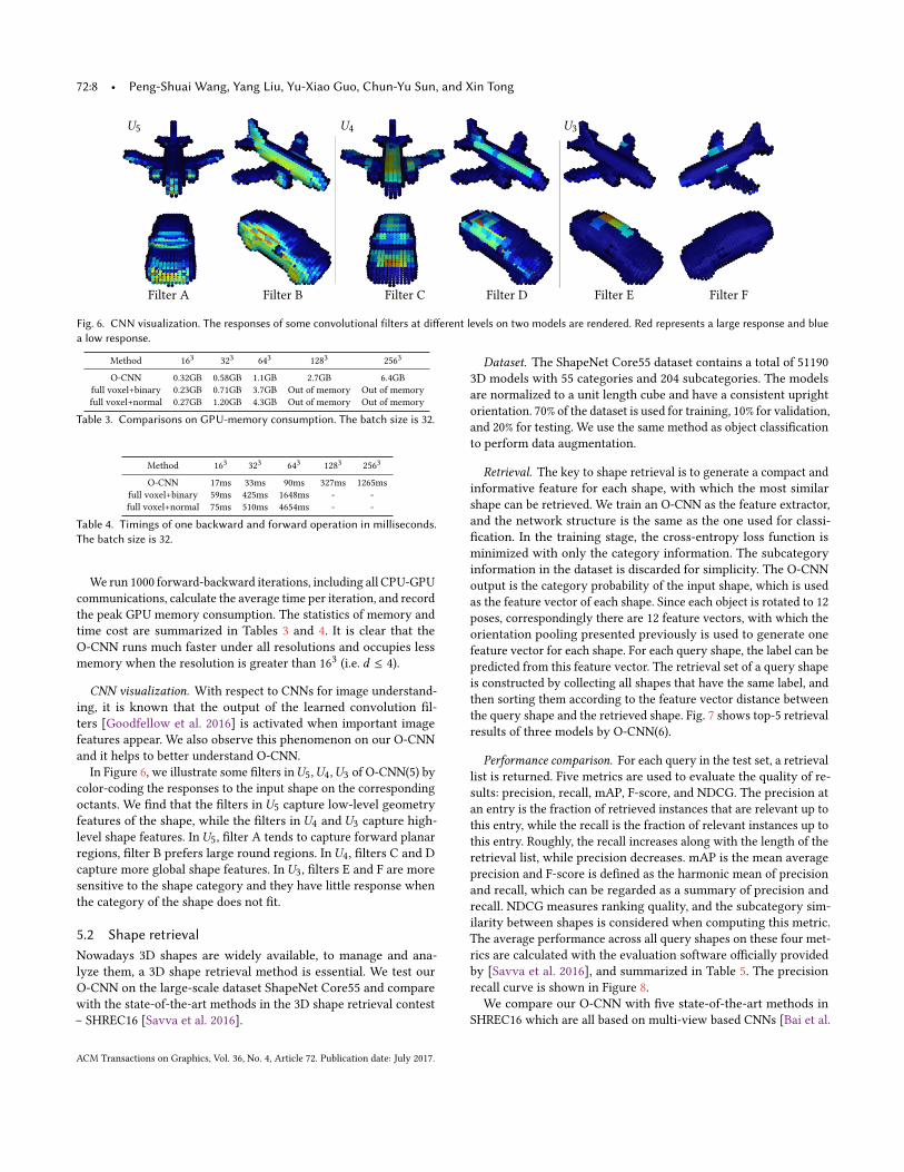
Filter A Filter B Filter C Filter D Filter E Filter F
U5 U4 U3
Fig. 6. CNN visualization. The responses of some convolutional filters at different levels on two models are rendered. Red represents a large response and bluea low response.
Method 163 323 643 1283 2563
O-CNN 0.32GB 0.58GB 1.1GB 2.7GB 6.4GBfull voxel+binary 0.23GB 0.71GB 3.7GB Out of memory Out of memoryfull voxel+normal 0.27GB 1.20GB 4.3GB Out of memory Out of memory
Table 3. Comparisons on GPU-memory consumption. The batch size is 32.
Table 4. Timings of one backward and forward operation in milliseconds.The batch size is 32.
We run 1000 forward-backward iterations, including all CPU-GPUcommunications, calculate the average time per iteration, and recordthe peak GPU memory consumption. The statistics of memory andtime cost are summarized in Tables 3 and 4. It is clear that theO-CNN runs much faster under all resolutions and occupies lessmemory when the resolution is greater than 163 (i.e. d ≤ 4).
CNN visualization. With respect to CNNs for image understand-ing, it is known that the output of the learned convolution fil-ters [Goodfellow et al. 2016] is activated when important imagefeatures appear. We also observe this phenomenon on our O-CNNand it helps to better understand O-CNN.
In Figure 6, we illustrate some filters inU5,U4,U3 of O-CNN(5) bycolor-coding the responses to the input shape on the correspondingoctants. We find that the filters in U5 capture low-level geometryfeatures of the shape, while the filters in U4 and U3 capture high-level shape features. InU5, filter A tends to capture forward planarregions, filter B prefers large round regions. InU4, filters C and Dcapture more global shape features. InU3, filters E and F are moresensitive to the shape category and they have little response whenthe category of the shape does not fit.
5.2 Shape retrievalNowadays 3D shapes are widely available, to manage and ana-lyze them, a 3D shape retrieval method is essential. We test ourO-CNN on the large-scale dataset ShapeNet Core55 and comparewith the state-of-the-art methods in the 3D shape retrieval contest– SHREC16 [Savva et al. 2016].
Dataset. The ShapeNet Core55 dataset contains a total of 511903D models with 55 categories and 204 subcategories. The modelsare normalized to a unit length cube and have a consistent uprightorientation. 70% of the dataset is used for training, 10% for validation,and 20% for testing. We use the same method as object classificationto perform data augmentation.
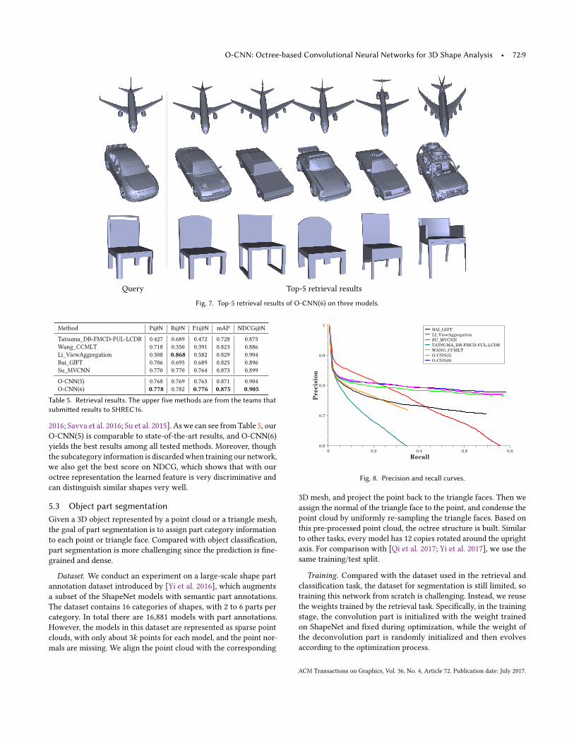
Retrieval. The key to shape retrieval is to generate a compact andinformative feature for each shape, with which the most similarshape can be retrieved. We train an O-CNN as the feature extractor,and the network structure is the same as the one used for classi-fication. In the training stage, the cross-entropy loss function isminimized with only the category information. The subcategoryinformation in the dataset is discarded for simplicity. The O-CNNoutput is the category probability of the input shape, which is usedas the feature vector of each shape. Since each object is rotated to 12poses, correspondingly there are 12 feature vectors, with which theorientation pooling presented previously is used to generate onefeature vector for each shape. For each query shape, the label can bepredicted from this feature vector. The retrieval set of a query shapeis constructed by collecting all shapes that have the same label, andthen sorting them according to the feature vector distance betweenthe query shape and the retrieved shape. Fig. 7 shows top-5 retrievalresults of three models by O-CNN(6).
Performance comparison. For each query in the test set, a retrievallist is returned. Five metrics are used to evaluate the quality of re-sults: precision, recall, mAP, F-score, and NDCG. The precision atan entry is the fraction of retrieved instances that are relevant up tothis entry, while the recall is the fraction of relevant instances up tothis entry. Roughly, the recall increases along with the length of theretrieval list, while precision decreases. mAP is the mean averageprecision and F-score is defined as the harmonic mean of precisionand recall, which can be regarded as a summary of precision andrecall. NDCG measures ranking quality, and the subcategory sim-ilarity between shapes is considered when computing this metric.The average performance across all query shapes on these four met-rics are calculated with the evaluation software officially providedby [Savva et al. 2016], and summarized in Table 5. The precisionrecall curve is shown in Figure 8.We compare our O-CNN with five state-of-the-art methods in
SHREC16 which are all based on multi-view based CNNs [Bai et al.
ACM Transactions on Graphics, Vol. 36, No. 4, Article 72. Publication date: July 2017.
O-CNN: Octree-based Convolutional Neural Networks for 3D Shape Analysis • 72:9
Query Top-5 retrieval results
Fig. 7. Top-5 retrieval results of O-CNN(6) on three models.
Table 5. Retrieval results. The upper five methods are from the teams thatsubmitted results to SHREC16.
2016; Savva et al. 2016; Su et al. 2015]. Aswe can see fromTable 5, ourO-CNN(5) is comparable to state-of-the-art results, and O-CNN(6)yields the best results among all tested methods. Moreover, thoughthe subcategory information is discardedwhen training our network,we also get the best score on NDCG, which shows that with ouroctree representation the learned feature is very discriminative andcan distinguish similar shapes very well.
5.3 Object part segmentationGiven a 3D object represented by a point cloud or a triangle mesh,the goal of part segmentation is to assign part category informationto each point or triangle face. Compared with object classification,part segmentation is more challenging since the prediction is fine-grained and dense.
Dataset. We conduct an experiment on a large-scale shape partannotation dataset introduced by [Yi et al. 2016], which augmentsa subset of the ShapeNet models with semantic part annotations.The dataset contains 16 categories of shapes, with 2 to 6 parts percategory. In total there are 16,881 models with part annotations.However, the models in this dataset are represented as sparse pointclouds, with only about 3k points for each model, and the point nor-mals are missing. We align the point cloud with the corresponding
3D mesh, and project the point back to the triangle faces. Then weassign the normal of the triangle face to the point, and condense thepoint cloud by uniformly re-sampling the triangle faces. Based onthis pre-processed point cloud, the octree structure is built. Similarto other tasks, every model has 12 copies rotated around the uprightaxis. For comparison with [Qi et al. 2017; Yi et al. 2017], we use thesame training/test split.
Training. Compared with the dataset used in the retrieval andclassification task, the dataset for segmentation is still limited, sotraining this network from scratch is challenging. Instead, we reusethe weights trained by the retrieval task. Specifically, in the trainingstage, the convolution part is initialized with the weight trainedon ShapeNet and fixed during optimization, while the weight ofthe deconvolution part is randomly initialized and then evolvesaccording to the optimization process.
ACM Transactions on Graphics, Vol. 36, No. 4, Article 72. Publication date: July 2017.
72:10 • Peng-Shuai Wang, Yang Liu, Yu-Xiao Guo, Chun-Yu Sun, and Xin Tong
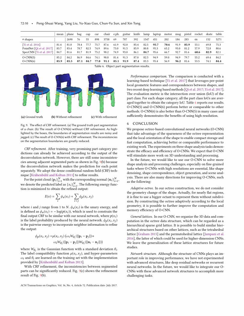
mean plane bag cap car chair e.ph. guitar knife lamp laptop motor mug pistol rocket skate table
(a) Ground truth (b)Without refinement (c)With refinement
Fig. 9. The effect of CRF refinement. (a) The ground truth part segmentationof a chair. (b) The result of O-CNN(6) without CRF refinement. As high-lighted by the boxes, the boundaries of segmentation results are noisy andjagged. (c) The result of O-CNN(6) with CRF refinement. The inconsistencieson the segmentation boundaries are greatly reduced.
CRF refinement. After training, very promising part category pre-dictions can already be achieved according to the output of thedeconvolution network. However, there are still some inconsisten-cies among adjacent segmented parts as shown in Fig. 9(b) becausethe deconvolution network makes the prediction for each pointseparately. We adopt the dense conditional random field (CRF) tech-nique [Krähenbühl and Koltun 2011] to refine results.
For the point cloud {pi }Ni=1 with the corresponding normal {ni }Ni=1,we denote the predicted label as {xi }Ni=1. The following energy func-tion is minimized to obtain the refined output:
E(x) =∑iϕu (xi ) +
∑i<j
ϕp (xi ,x j )
where i and j range from 1 to N . ϕu (xi ) is the unary energy, andis defined as ϕu (xi ) = − log(p(xi )), which is used to constrain thefinal output CRF to be similar with our neural network, where p(xi )is the label probability produced by the neural network. ϕp (xi ,x j )is the pairwise energy to incorporate neighbor information to refinethe output:
ϕp (xi ,x j ) =µ(xi ,x j )(ω1Wθ1 (∥pi − pj ∥)+
ω2Wθ2 (∥pi − pj ∥)Wθ3 (∥ni − nj ∥))
whereWθi is the Gaussian function with a standard deviation θi .The label compatibility function µ(xi ,x j ), and hyper-parametersωi and θi are learned on the training set with the implementationprovided by [Krähenbühl and Koltun 2013].With CRF refinement, the inconsistencies between segmented
parts can be significantly reduced. Fig. 9(c) shows the refinementresult of Fig. 9(b).
Performance comparison. The comparison is conducted with alearning-based technique [Yi et al. 2017] that leverages per-pointlocal geometric features and correspondences between shapes, andtwo recent deep learning basedmethods [Qi et al. 2017; Yi et al. 2017].The evaluation metric is the intersection over union (IoU) of thepart class. For each shape category, all the part class IoUs are aver-aged together to obtain the category IoU. Table 6 reports our results.O-CNN(5) and O-CNN(6) perform better or comparable to othermethods. O-CNN(6) is also better than O-CNN(5) in many cases andsufficiently demonstrates the benefits of using high resolution.
6 CONCLUSIONWe propose octree-based convolutional neural networks (O-CNN)that take advantage of the sparseness of the octree representationand the local orientation of the shape to enable compact storage andfast computation, achieving better or comparable performance toexistingwork. The experiments on three shape analysis tasks demon-strate the efficacy and efficiency of O-CNNs. We expect that O-CNNwill stimulate more work on 3D understanding and processing.
In the future, we would like to use our O-CNN to solve moreshape analysis and processing challenges, especially on fine-grainedtasks where O-CNNs with high resolutions are essential, like shapedenoising, shape correspondence, object generation, and scene anal-ysis. There are also many directions for improving O-CNNs, suchas the following:
Adaptive octree. In our octree construction, we do not considerthe geometry change of the shape. Actually, for nearly flat regions,it is fine to use a bigger octant to represent them without subdivi-sion. By constructing the octree adaptively according to the localgeometry, it is possible to further improve the computation andmemory efficiency of O-CNN.
General lattices. In our O-CNN, we organize the 3D data and com-putation in the octree data structure, which can be regarded as ahierarchical sparse grid lattice. It is possible to build similar hier-archical structures based on other lattices, such as the tetrahedrallattice [Graham 2015] and the permutohedral lattice [Jampani et al.2016], the latter of which could be used for higher-dimension CNNs.We leave the generalization of these lattice structures for futurestudies.
Network structure. Although the structure of CNNs plays an im-portant role in improving performance, we have not experimentedwith advanced structures, like deep residual networks or recurrentneural networks. In the future, we would like to integrate our O-CNNs with these advanced network structures to accomplish morechallenging tasks.
ACM Transactions on Graphics, Vol. 36, No. 4, Article 72. Publication date: July 2017.
O-CNN: Octree-based Convolutional Neural Networks for 3D Shape Analysis • 72:11
ACKNOWLEDGMENTSWe wish to thank the authors of [Chang et al. 2015; Wu et al. 2015]for sharing their 3D model datasets with the public, the authorsof [Qi et al. 2017; Yi et al. 2016] for providing their evaluationdetails, Stephen Lin for proofreading the paper, and the anonymousreviewers for their constructive feedback.
REFERENCESSong Bai, Xiang Bai, Zhichao Zhou, Zhaoxiang Zhang, and Longin Jan Latecki. 2016.
GIFT: A real-time and scalable 3D shape search engine. In Computer Vision andPattern Recognition (CVPR).
D. Boscaini, J. Masci, S. Melzi, M. M. Bronstein, U. Castellani, and P. Vandergheynst.2015. Learning class-specific descriptors for deformable shapes using localizedspectral convolutional networks. Comput. Graph. Forum 34, 5 (2015), 13–23.
Davide Boscaini, Jonathan Masci, Emanuele Rodolà, and Michael M. Bronstein. 2016.Learning shape correspondence with anisotropic convolutional neural networks. InNeural Information Processing Systems (NIPS).
Andrew Brock, Theodore Lim, J.M. Ritchie, and Nick Weston. 2016. Generative anddiscriminative voxel modeling with convolutional neural networks. In 3D deeplearning workshop (NIPS).
M. M. Bronstein, J. Bruna, Y. LeCun, A. Szlam, and P. Vandergheynst. 2017. Geometricdeep learning: going beyond Euclidean data. IEEE Sig. Proc. Magazine (2017).
Angel X. Chang, Thomas Funkhouser, Leonidas Guibas, Pat Hanrahan, Qixing Huang,Zimo Li, Silvio Savarese, Manolis Savva, Shuran Song, Hao Su, Jianxiong Xiao,Li Yi, and Fisher Yu. 2015. ShapeNet: an information-rich 3D model repository.arXiv:1512.03012 [cs.GR]. (2015).
Kumar Chellapilla, Sidd Puri, and Patrice Simard. 2006. High performance convolutionalneural networks for document processing. In International Conference on Frontiersin Handwriting Recognition (ICFHR).
Ian Goodfellow, Yoshua Bengio, and Aaron Courville. 2016. Deep Learning. MIT Press.Ben Graham. 2015. Sparse 3D convolutional neural networks. In British Machine Vision
Conference (BMVC).Kan Guo, Dongqing Zou, and Xiaowu Chen. 2015. 3D mesh labeling via deep convolu-
tional neural networks. ACM Trans. Graph. 35, 1 (2015), 3:1–3:12.Varun Jampani, Martin Kiefel, and Peter V. Gehler. 2016. Learning sparse high dimen-
sional filters: image filtering, dense CRFs and bilateral neural networks. In ComputerVision and Pattern Recognition (CVPR).
Yangqing Jia, Evan Shelhamer, Jeff Donahue, Sergey Karayev, Jonathan Long, RossGirshick, Sergio Guadarrama, and Trevor Darrell. 2014. Caffe: convolutional archi-tecture for fast feature embedding. In ACM Multimedia (ACMMM). 675–678.
Philipp Krähenbühl and Vladlen Koltun. 2011. Efficient inference in fully connectedCRFs with gaussian edge potentials. InNeural Information Processing Systems (NIPS).
Philipp Krähenbühl and Vladlen Koltun. 2013. Parameter learning and convergentinference for dense random fields. In International Conference on Machine Learning(ICML). 513–521.
Y. Lecun, L. Bottou, Y. Bengio, and P. Haffner. 1998. Gradient-based learning applied todocument recognition. Proc. IEEE 86, 11 (1998), 2278–2324.
Yangyan Li, Soeren Pirk, Hao Su, Charles R. Qi, and Leonidas J. Guibas. 2016. FPNN:field probing neural networks for 3D data. In Neural Information Processing Systems(NIPS).
Sergey Loffe and Christian Szegedy. 2015. Batch Normalization: accelerating deepnetwork training by reducing internal covariate shift. In International Conference onMachine Learning (ICML). 448–456.
Jonathan Long, Evan Shelhamer, and Trevor Darrell. 2015. Fully convolutional modelsfor semantic segmentation. In Computer Vision and Pattern Recognition (CVPR).
JonathanMasci, Davide Boscaini, Michael M. Bronstein, and Pierre Vandergheynst. 2015.Geodesic convolutional neural networks on Riemannian manifolds. In InternationalConference on Computer Vision (ICCV).
D. Maturana and S. Scherer. 2015. VoxNet: a 3D convolutional neural network forreal-time object recognition. In International Conference on Intelligent Robots andSystems (IROS).
Donald Meagher. 1982. Geometric modeling using octree encoding. Computer Graphicsand Image Processing 19 (1982), 129–147.
Hyeonwoo Noh, Seunghoon Hong, and Bohyung Han. 2015. Learning deconvolutionnetwork for semantic segmentation. In International Conference on Computer Vision(ICCV). 1520–1528.
Charles R. Qi, Hao Su, Kaichun Mo, and Leonidas J. Guibas. 2017. PointNet: Deeplearning on point sets for 3D classification and segmentation. In Computer Visionand Pattern Recognition (CVPR).
Charles Ruizhongtai Qi, Hao Su, Matthias Nießner, Angela Dai, Mengyuan Yan, andLeonidas J. Guibas. 2016. Volumetric and multi-view CNNs for object classificationon 3D data. In Computer Vision and Pattern Recognition (CVPR).
Gernot Riegler, Ali Osman Ulusoy, and Andreas Geiger. 2017. OctNet: Learning deep3D representations at high resolutions. In Computer Vision and Pattern Recognition(CVPR).
M. Savva, F. Yu, Hao Su, M. Aono, B. Chen, D. Cohen-Or, W. Deng, Hang Su, S. Bai, X.Bai, N. Fish, J. Han, E. Kalogerakis, E. G. Learned-Miller, Y. Li, M. Liao, S. Maji, A.Tatsuma, Y. Wang, N. Zhang, and Z. Zhou 4. 2016. SHREC’16 Track – Large-scale3D shape retrieval from ShapeNet Core55. In Eurographics Workshop on 3D ObjectRetrieval.
B. Shi, S. Bai, Z. Zhou, and X. Bai. 2015. DeepPano: deep panoramic representation for3-D shape recognition. IEEE Signal Processing Letters 22, 12 (2015), 2339–2343.
Ayan Sinha, Jing Bai, and Karthik Ramani. 2016. Deep learning 3D shape surfaces usinggeometry images. In European Conference on Computer Vision (ECCV). 223–240.
Nitish Srivastava, Geoffrey E Hinton, Alex Krizhevsky, Ilya Sutskever, and RuslanSalakhutdinov. 2014. Dropout: a simple way to prevent neural networks fromoverfitting. Journal of Machine Learning Research 15, 1 (2014), 1929–1958.
H. Su, S. Maji, E. Kalogerakis, and E. Learned-Miller. 2015. Multi-view convolutionalneural networks for 3D shape recognition. In International Conference on ComputerVision (ICCV).
Jane Wilhelms and Allen Van Gelder. 1992. Octrees for faster isosurface generation.ACM Trans. Graph. 11, 3 (1992), 201–227.
Z. Wu, S. Song, A. Khosla, F. Yu, L. Zhang, X. Tang, and J. Xiao. 2015. 3D ShapeNets: Adeep representation for volumetric shape modeling. In Computer Vision and PatternRecognition (CVPR).
Li Yi, Vladimir G. Kim, Duygu Ceylan, I-Chao Shen, Mengyan Yan, Hao Su, Cewu Lu,Qixing Huang, Alla Sheffer, and Leonidas Guibas. 2016. A scalable active frameworkfor region annotation in 3D shape collections. ACM Trans. Graph. (SIGGRAPH ASIA)35, 6 (2016), 210:1–210:12.
Li Yi, Hao Su, Xingwen Guo, and Leonidas Guibas. 2017. SyncSpecCNN: synchronizedspectral CNN for 3D shape segmentation. In Computer Vision and Pattern Recognition(CVPR).
Matthew D. Zeiler and Rob Fergus. 2014. Visualizing and understanding convolutionalnetworks. In European Conference on Computer Vision (ECCV).
Kun Zhou, Minmin Gong, Xin Huang, and Baining Guo. 2011. Data-parallel octrees forsurface reconstruction. IEEE. T. Vis. Comput. Gr. 17, 5 (2011), 669–681.
ACM Transactions on Graphics, Vol. 36, No. 4, Article 72. Publication date: July 2017.