O n th e p rop erties of sim ilarity su b grid -scale …rstoll/LES/Handouts/Liu_etal_JFM94.pdfK...

J . Fluid Mech. (1994), uol. 215, pp . 83-1 19 Copyright 0 1994 Cambridge University Press

83

On the properties of similarity subgrid-scale models as deduced from measurements in a turbulent jet

By SHEWEN LIU, CHARLES MENEVEAU A N D JOSEPH KATZ

Department of Mechanical Engineering, The Johns Hopkins University, Baltimore, MD 21218, USA

(Received 19 November 1993 and in revised form 7 March 1994)

The properties of turbulence subgrid-scale stresses are studied using experimental data in the far field of a round jet, at a Reynolds number of R, z 310. Measurements are performed using two-dimensional particle displacement velocimetry. Three elements of the subgrid-scale stress tensor are calculated using planar filtering of the data. Using a priori testing, eddy-viscosity closures are shown to display very little correlation with the real stresses, in accord with earlier findings based on direct numerical simulations at lower Reynolds numbers. Detailed analysis of subgrid energy fluxes and of the velocity field decomposed into logarithmic bands leads to a new similarity subgrid- scale model. It is based on the ‘resolved stress’ tensor L,,, which is obtained by filtering products of resolved velocities at a scale equal to twice the grid scale. The correlation coefficient of this model with the real stress is shown to be substantially higher than that of the eddy-viscosity closures. It is shown that mixed models display similar levels of correlation. During the a priori test, care is taken to only employ resolved data in a fashion that is consistent with the information that would be available during large- eddy simulation. The influence of the filter shape on the correlation is documented in detail, and the model is compared to the original similarity model of Bardina et al. (1980). A relationship between L,, and a nonlinear subgrid-scale model is established. In order to control the amount of kinetic energy backscatter, which could potentially lead to numerical instability, an ad hoc weighting function that depends on the alignment between Lii and the strain-rate tensor, is introduced. A ‘dynamic’ version of the model is shown, based on the data, to allow a self-consistent determination of the coefficient. In addition, all tensor elements of the model are shown to display the correct scaling with normal distance near a solid boundary.

1. Introduction An important problem for the large-eddy simulation (LES) of turbulent flows is the

parametrization of the subgrid scales as a function of the resolved flow variables. This problem has been receiving considerable attention in recent years owing to the increasing possibilities of engineering applications of LES (see e.g. Akselvoll & Moin 1993 and other contributions appearing in that volume), and owing to recent developments in modelling (German0 et al. 1991; Lilly 1992; Piomelli 1993 among others).

The basic concepts and initial experiments with LES are described in Smagorinsky (1963), Lilly (1967) and Deardorff (1970). Further developments and applications can be found in Schumann (1975), Ferziger (1977), Clark, Ferziger & Reynolds (1979), Bardina, Ferziger & Reynolds (1980), Piomelli, Moin & Ferziger (1988), Yoshizawa

84 S . Liu, C. Meneveau and J. Katz

(1989), Schmidt & Schumann (1989), Mktais & Lesieur (1992), and Horiuti (1993). For analytical treatments of subgrid-scale (SGS) modelling, see e.g. Leonard (1974), Kraichnan (1976), Leslie & Quarini (1979), Chollet & Lesieur (1981), Chasnov (1981). Rogallo & Moin (1984) and Reynolds (1990) give reviews of the field.

Let us consider an incompressible turbulent flow obeying the Navier-Stokes equations. It follows that Gi(x, t ) the convolution (denoted by a tilde) of the velocity field with some spatial filter of characteristic width d (or some anisotropic filter with widths di in each direction, i = 1,2,3), obeys the filtered Navier-Stokes equations

az? . 2 = 0, axi

The SGS stress tensor rii is defined as

where, on purpose, we have not subtracted the trace. In order to successfully solve (2) on a computational mesh with a grid size of the order of A , one needs to parametrize T J X , t ) in terms of the resolved velocity field G,(x, t). We shall denote such a model by the tensor qJlZ].

One method of investigating the correctness of an SGS model is to perform the simulation for a particular flow and then compare the results with experimental data (commonly referred to as a posteriori model testing, as coined in Piomelli et al. 1988). Another approach consists of using fully resolved velocity fields to compare the local instantaneous subgrid stress with the prediction of a subgrid-scale model. This approach, frequently called a priori testing (Piomelli et al. 1988), was pioneered by Clarke et al. (1979) and McMillan & Ferziger (1979) through the analysis of fields obtained from direct numerical simulations (DNS). With this approach, it has been repeatedly observed that the eddy-viscosity closures in general, and the Smagorinsky model

9-13") = - 2(c, 4)2 151 SZl (4)

in particular, display very little correlation with the real stress T , ~ . On a local and instantaneous basis, these two tensors are almost never the same. Nevertheless, this need not be a problem per se for the LES prediction of the correct flow statistics, and the relative success of LES in this regard points to considerable robustness of the LES equations. Meneveau (1994) derived a set of necessary conditions on the modelled stress that make correct LES statistics possible, and showed, in grid turbulence, that eddy-viscosity closures do follow these conditions surprisingly well.

On the other hand, a model which could be shown to also display a high correlation between rtJ and Ti during a priori tests would be more desirable. Among other things, the predictability of individual flow realizations could be enhanced with instan- taneously more realistic models. Such a feature is of relevance to, for example, active control of turbulent flow. Along these lines, it can be argued that the most well-known model to have resulted from a priori analysis of DNS data is the similarity model of Bardina et a/. (1980). Using the observation that the filtered value of the fluctuating velocity u: = u, - z?, can be written as

( 5 ) -, * z u, = u, - u,

The properties of similarity subgrid-scale models 85

it was postulated that qj, the SGS Reynolds stress (= q), could be approximated as

(6) After a similar argument is made for the cross-stresses, and after addition of the Leonard stress, the Bardina similarity model reads

This model (and several of its variants) has been repeatedly shown to exhibit considerable correlation with the real stress during a priori tests (Bardina et al. 1980; Piomelli et al. 1988; Horiuti 1989, etc.). However, when implemented in LES calculations, the addition of eddy-viscosity terms was always found to be necessary in order for sufficient energy dissipation to take place.

A fundamental drawback of a priori analysis based on DNS data is the restriction to low Reynolds numbers. Thus both of the above conclusions (low correlation coefficients for eddy-viscosity closures and high correlations for the Bardina model) are based on data that are representative of high-Reynolds-number flows only under relatively strong assumptions. To overcome this difficulty, one can consider experimental data, where substantially higher Reynolds numbers and/or more complex flows can be considered. Experimental data are not without their problems, however, as only partial information about the flow is accessible, depending on the measurement technique.

The present work is an experimental a priori study of SGS modelling. The choice of what type of flow to study is dictated by the need to consider as high a Reynolds number as possible. The far field of a jet provides reasonably high Reynolds numbers (we will find R, - 3 10) within a moderately sized facility. This is unlike grid-generated turbulence, where relatively low fluctuating velocities typically lead to lower microscale Reynolds numbers. The next important step in the proposed methodology is to obtain as complete information about the flow field as possible. The technique of particle displacement velocimetry (PDV) allows us, at present, to measure the projection of the velocity vectors onto two-dimensional sections of the flow. The experimental set-up and the instrumentation are described in $2. In $3, the data's kinetic energy spectrum is documented, and we verify that we are adequately resolving the inertial-range scales of interest. Section 4 describes a study of the Smagorinsky model and of the rate of kinetic energy dissipation accomplished by the SGS stress. We then study the energy flux to different ranges of small scales, which motivates us to perform a decomposition of the velocity field into distinct bands.

In $45 and 6 a systematic study of flow features at different lengthscales is used to propose a new similarity SGS model. The correlation coefficient between this similarity model and the real stress is measured, and the influence of different filters is documented. Particular emphasis is placed on performing the analysis using only data that are consistent with that available during an LES (an approach which we shall call a consistent a priori test). The tests are made more complete by comparatively applying them to Gaussian fields with random phases, displaying a white-noise or a -: energy spectrum.

After having established these basic results from the experimental data, in the next sections (7-9) we discuss some of the properties of the model and propose some possible modifications. There, the experimental data are used to support and illustrate the discussion rather than to arrive at the results. First we establish connections to nonlinear models based on the resolved velocity-gradient tensor ($7). Second, in $8, we introduce a means of controlling the amount of backscatter, and amend the similarity model derived before. This ad hoc modification yields a dissipative similarity model.

Bij = ( Ci - Gi) ( Cj - Cj) .

yw $9 = r n . - C , 2 9 u".. (7)

86 S. Liu, C. Meneveau and J. Katz

Application of the dynamic procedure of German0 et al. (1991) and the near-wall scaling of the SGS stress are discussed in $9. A summary of the results and the basic conclusions are given in $ 10.

2. Experimental set-up 2.1. Facility

As noted before, our objective is to generate turbulent flow with R, as high as possible, but within a moderately sized facility. Of the possibilities considered, the far field of a turbulent jet seems to be the simplest and most flexible option. A schematic description of the test facility is presented in figure 1 (a). It consists of a water jet of diameter D = 6.3 mm, which is injected into a 71 x 71 cm wide and 183 cm long chamber that has windows on all sides. Turning vanes, honeycomb and screens, as well as a smooth cosine shaped nozzle are used for control of turbulence and uniformity of the jet. A large honeycomb at the bottom of the chamber is used for reducing the effect of the exit pipe. The flow is driven by a f hp centrifugal pump, that is attached to the rest of the facility with 1 m long flexible hoses to reduce the impact of vibrations. The available power of the pump enables injection speeds of up to 18 m s-' at the nozzle. The experiments are performed at 15 m s-l (Re, = 9.5 x lo'). All the measurements are performed in the centreplane of the facility. The square, 7 x 7 cm, sample area is centred 193 diameters downstream of the nozzle. Its size ( L = 7 cm) is chosen to approximately match the integral scale of turbulence at this downstream location. Employing the usual estimates for a round jet (Tennekes & Lumley 1972), the flow integral scale at x , / D = 193 is 1 M 7 cm.

2.2. Instrumentation Velocity measurements are performed using particle displacement velocimetry. A schematic description of the optical set-up is presented in figure 1 (b). The light source is a 30 W copper vapour laser (out of which about 20 W are green - 51 1.5 nm, and 10 W are yellow - 578 nm). A dichroic filter is used to filter out the yellow beam, which enables better focusing into a narrow sheet. The beam diameter is reduced to about 1 mm and then expanded into a thin sheet with a cylindrical lens. To obtain acceptable levels of resolution, the images are recorded by a Hasseblad film camera, which has an image size of 56 x 56 mm on the film. It is equipped with a 120 mm lens and extension tubes, which enables the recording of data at a magnification factor of 0.65. Thus, the image covers an area of 8.6 x 8.6 cm, out of which 7 x 7 cm are used during the analysis. Photographs are recorded on TMAX ASA 3200 film. Coordination between the camera and the laser is achieved using a control system (Ganapathy & Katz 1993) hosted by a personal computer. Typically, triple-exposure images are recorded. The duration of each laser pulse is 40ns, and the delay between pulses is 0.675 ms. Spherical fluorescent particles, 20 pm in diameter, are used as velocity tracers (Dong, Chu & Katz 1992). These particles are manufactured in our laboratory and have a specific gravity ranging between 0.95 and 1.1. At this size, and owing to the velocities involved, the relative velocity between the particles and the fluid is insignificant. The entire facility is flooded with these particles.

The negatives are scanned using a Nikon LS 3500, 35 mm slide scanner. Owing to its large size, each negative must be scanned in six separate portions. These portions are then matched, by comparing the location of several particles chosen as reference. The error introduced through this procedure is negligible. Overall, each negative is converted to a 5000 x 5000 pixels array, which is then filtered and enhanced. The


(b) 1 mm Laser sheet

Tank:

view

I M C Copper vapour laser

FIGURE 1. Schematic of the experimental set-up. The facility is shown in (a): 1, tank; 2, nozzle ( D = 0.635 cm); 3, honeycomb; 4, filter; 5, flexible hose; 6, pump; 7, speed control; 8, honeycomb & screen. All dimensions are in cm. The optical instrumentation is shown in (b) : M, mirror; SL, spherical lens; CL, cylindrical lens; F, filter.

autocorrelation method, described in detail by Dong et al. (1992) is used for computing the velocity. Each vector is determined from a 64 x 64 pixels array, which corresponds to a 1.1 x 1.1 mm window in the actual flow field. The velocity is evaluated every 32 pixels (the smallest grid spacing, denoted by d), which means that 50 YO of neighbouring windows overlap. Sub-pixel accuracy (about 0.2 pixels) is achieved by interpolating between the discretely computed values of the auto-correlation function. Problems occur occasionally (in less than 0.3 YO of the windows) when the particle density is low, or when a particularly bright particle is present. To correct for these cases, the analysis procedure includes detailed comparisons between neighbouring vectors. Whenever their difference exceeds a pre-determined threshold, the correlation peaks are recalculated using either enlarged or slightly shifted windows. Only images where every vector can be determined, corrected or corroborated in this fashion, are used in the present study. No interpolation is employed to make up for incomplete data.

Based on calibration experiments performed by Dong et al. (1992), the error in our method is about 1 YO of the velocity, provided each interrogation window contains at least 8 particle pairs. This requirement dictates the required particle density in the test facility, of at least 7 mm-3. The corresponding volume fraction, < 0.003 YO, is still below any level that affects the flow structure and turbulence characteristics.

88 S. Liu, C. Meneveau and J . Katz

6

4

2

0

0 2 4 x1 (cm>

6

FIGURE 2. Instantaneous velocity vectors projected onto an axial plane in the far field of a turbulent round jet. There are 128 x 128 vectors. The mean velocity of the image (shown on the top right) is from right to left, and has been subtracted from each vector. The velocity scale is indicated on the top left.

Computations are performed on an IBM RS/6000 workstation. On this computer it typically takes about 30 minutes to calculate 2000 vectors from an 8 bit image, including data evaluation, comparison to neighbouring vectors etc. Thus, a single vector map containing 128 x 128 vectors takes about 4 hours CPU time to analyse. In the present paper we have opted to present results obtained from six images.

3. Flow characterization In this section, the basic features of the flow are described. Figure 2 is a typical

velocity map after the mean velocity has been subtracted. The mean velocity, computed over the entire image, is in the -x, direction. Turbulent motion is visible over a wide range of lengthscales. This feature is illustrated by considering the portion of the flow enclosed in the square, which is shown in figure 3 in an enlarged format. Although the jet continues to develop from the right to the left portion of the imaged region, in the present study we neglect the spatial inhomogeneity of the flow statistics within the

The properties of similarity subgrid-scale models

+ 0.5 m SKI

89

2.5 3.0 3.5 4.0

XI (cm) FIGURE 3 . Enlarged portion of figure 2, showing details of the turbulent flow field.

image. This approximation is warranted since the changes in mean quantities are small compared to the turbulence quantities (e.g. according to usual estimates the mean and root-mean-square velocities at the centreline will change only by about 5 YO). Therefore we accumulate statistics over the entire image (excepting some regions close to the edges, as explained later). Furthermore, in order to improve statistical convergence, six images will be employed for all averages presented in this paper, unless stated otherwise.

The mean streamwise velocity in the imaged region is Urn,,, = - 0.5 m s-l, while the velocity root-mean-square (r.m.s.) values in the streamwise and transverse directions are u; = u; = 0.09 m s-l. The dissipation rate per unit mass, estimated as e M u;3/1, is e M 0.01 1 m2 sc3. An estimate for the average value of the Kolmogorov scale in the region of interest is 7 = ( v ' / ~ ) ' / ~ M 0.1 mm. The Taylor microscale is estimated by h M u ; ( 1 5 v / ~ ) ~ / ~ M 3.4 mm. Therefore, the microscale Reynolds number is R, z 310, which is considerably higher than that of DNS data sets that have been previously employed to study SGS models.

The spectral properties of the flow are now described. We consider the radial two- dimensional spectrum, defined by a sum over an annulus with radius k in wavenumber mace :

is the two-dimensional Fourier transform of the velocity field in the plane x, = [x,],. Furthermore,

is a (Welch) windowing function which is needed because the data are not periodic. The

90 2;. Liu. C. Meneveau and J . Katz

- w

1 0 3 1

FIGURE 4. (a) Radial two-dimensional energy spectrum in Kolmogorov units, of the vector field shown in figure 2 . Circles and squares are for the u1 and u2 components, respectively. Lines show the Kolmogorov spectrum (without a dissipation range), for C, = 1.6 (dotted line) and C, = 2 (solid line). (b) Same as (a), but averaged over all six images.

spectrum that results from the velocity field of figure 2 is shown in figure 4(a), in Komolgorov units. For comparison, the solid and dotted lines show the inertial-range behaviour of the Kolmogorov spectrum, E&) = PC, k 5 I 3 , for two different values of the Kolmogorov constant (C, = 2.0 and C, = 1.6). The coefficient /3 = 0.535 accounts for the fact that we are dealing with a two- and not a three-dimensional radial spectrum (see Appendix A). Several observations can readily be made. (i) A significant portion of the spectrum (over a decade) is consistent with a --g power-law decay. (ii) The implied value of the Kolmogorov constant (C, = 2.0) is within the range of accepted values, although on the high side. However, since this constant depends strongly on the estimate of e, which itself is very approximate, not much significance can be ascribed to the implied value of C,. (iii) Finally, the dissipation range is not resolved in these data, which is not surprising if we recall that our spatial resolution (given by the width of the sampling windows) is, by design, approximately 107. In order to eliminate some of the scatter in the spectrum, it can recomputed by averaging over all six images. The result is shown in figure 4(b), confirming that the above conclusions are valid for the ensemble as well. We now comment on the noise which is visible at high wavenumbers. An estimate of the expected level of the noise floor can be obtained by noticing that an experimental uncertainty of 1 % of the mean velocity translates in this case into an uncertainty of about 5 % of the r.m.s. velocity. Thus one can expect a noise floor at 0 . 0 P FZ 2.5 decades below the peak of the energy spectrum, consistent with the results in figure 4. This noise floor is not a serious limitation for the purposes of the present study, since we are interested in filtering the data at lengthscales pertaining to the inertial range and do not have any direct interest in the dissipative range.

4. Basic statistics of SGS stresses In this section we give some basic definitions related to the filtering. Also, the method

of calculating the subgrid stress is described, and we document some of its fundamental properties.

4.1. Definitions The filtered velocity field is formally defined as

J - c c J - r n


where l$(xl, x,) is a spatial low-pass filter with characteristic width A . We notice that the filtering is a two-dimensional one, instead of the three-dimensional filtering that is possible when analysing DNS data. We shall comment on the limitations and interpretation of this two-dimensional filtering in $4.2. The discrete filtering is performed using the fast Fourier transform on the measurement grid. The filters that will be employed are

top hat:

Gaussian : l$(xl, x,) = K, exp [ - 6(x; + xi)/A2] ;

cut-off: sin (nxl/A) sin (nx2/A)

nxl/A nx,/A * Fd(Xl,X,) = K3

The coefficient Kl is a normalization factor which ensures that the integral of the filter equals unity (in the discrete sense). With regard to end effects that need to be taken into account for the filtering, we adopt the following procedures. For the top-hat filter, we only analyse the data in an interior region of size L - A (recalling that L = 7 cm), so that no errors are generated at the boundaries. The other two filters (Gaussian and cut- off) have long tails. We adopt the following dual strategy. (i) The data are extended by assuming them to be symmetric with respect to the edges of the domain (u,(-xl,x2) = ui(xl, x,) and ui(L+ x,, x,) = ui(L-xl, x,), and similarly in the x, direction). In this manner, discontinuity of the data is avoided. (ii) Furthermore, statistics are accumulated only over an interior subset of size L-A, for which the edge effects are small. For the Gaussian filter, the truncated portion of the filter corresponds to a tail starting at x/A = 0.5. This tail contains only 4% of the total area under the filter function. For the cut-off filter (which we shall not use very frequently) we recognize that the errors involved are more significant because of its slow l /x decay.

A typical filtered velocity-vector field is shown in figure 5 , using the top-hat filter with a filter size of A = 86 - 489. As can be seen, the small-scale motion has been smoothed out.

Similarly, the SGS stress elements T~~ are computed according to a m

u~(x;, x;) u~(x;, x;) &(X, - x;, X, -xi) dxi dx; s_, J-, ~ij(x1, XJ =

- u"&, x,) qx , , x,) ( i , j = 1,2). (14)

= aqax,, (15)

sij = ;(A"ij + A",,), 3, = (Ll2 -A",,). (16)

The resolved velocity-gradient tensor xij is defined as w

while the resolved rate-of-strain elements and measured vorticity component are w

We will frequently use the fields zii and 7ij 'sampled' on a coarse mesh with a spacing of A . The nodes of this mesh are located at ([xx,],+jl A , [x,], +j, A ) , where (jl = 0,1,2, . . . ; j 2 = 0,1,2, . . . .), and where the point ([xl],, [x,],) is a reference point. Occasionally we shall consider averages over all possible reference points.

4.2. Interpretation of Jiltering In the context of the a priori analysis to follow in this paper, the measured values of Ci and T~~ will be employed quite frequently. It is therefore pertinent to give, at this point in the development, a precise interpretation of these variables.

92 S. Liu, C. Meneveau and J . Katz - 0.5 m SK'

4

2

0

FIGURE 5. Vector map of the filtered velocity lii. A top-hat filter was applied to the image shown in figure 2, with a width A = 86 - 48q, where S is the original grid size (0.55 mm) and q is the Kolmogorov scale. To avoid crowding, the figure shows every second vector only. The mean velocity and the fundamental velocity unit is shown on the top.

We start by assuming that a three-dimensional LES is being performed, using (for instance) a finite-volume formulation with rectangular cells. We denote the discrete LES velocity by u ~ ( j l , j 2 , j 3 ) , and assume that it represents the average velocity in the cell with centre located at ([x,], +j, A, , [x,], +j2 A, , [x,], +j, 4,). As a thought experiment, we now assume that at some instant in time the entire LES velocity field u:(j,,j,,j,) is set equal to the real field, Z2f(jl,jz,j3) which actually exists at location ([x,], +j, A,, [x,], +j, A,, [x,],, +j, A,) . The tilde denotes filtering with 4, a three- dimensional top-hat filter with widths Ai in each direction. We now argue that in order for the LES field to continue with a realistic time evolution (i.e. for u* to approximate Z2 at later times), its SGS model for the stress, q j [ u * ] (jl,j2,j3), should be equal (or as 'close' as possible) to the real stress tensor at these points, ~ ~ ~ ( j , , j , , j J .

Before proceeding with the main line of the argument, we make a connection with our present data by letting [x,], be the location of the data plane (with j , = 0). For simplicity, we now eliminate the reference to the x, direction. Furthermore, we assume that the grid resolution of the LES in the x, direction is very good (i.e. A , - 7 < A ) . In consequence, for the analysis of the real data we choose 4 to be a top-hat filter which is thin in the x3 direction, as is effectively the case in the experiment.

Based on the data, we can evaluate the tensor ri j ( j l , j2) as in (14). Since we are assuming that u: = uli at the grid points ( j l , j 2 ) , we can also compute

&k*l ( j l J Z ) = 4 j [ E I ( j l J 2 ) ,

if a particular form of qj as a function of the resolved velocity field is postulated (SGS model). A simple measure of the level of agreement between rij and qj is the correlation coefficient between the two fields. The reasoning which we shall adopt will


FIGURE 6. Schematic diagram showing the original grid (spacing = 8) and the coarse LES grid level (spacing = A). Consistent a priori testing requires that when comparing a model expression for the stress at point (jl,j,) with ro at that same point, the model is only allowed to employ information that is available on the coarse grid (solid circles). Only after the local comparison is made, can the reference location ([x,],, [x,],) for the coarse mesh be shifted by multiples of 6 to enlarge the statistical sample. The following expression is an example of box filtering at a scale 26:

ax110 + j l 4 [X,l, +j, 4 = @lJJ = afi,(j,J,, ++@,(jl,j2+ 1)+qj1,j ,- l )+ i t ( j l+ LjJ+qj,- I>j,)l +&{Gt(jl + lJ, + 1) + E t ( j l + 1, j,- 1)+ Gz(jl- 1 , j , + 1) +Et(jl - l,j,- 1)).

be that the higher this correlation is, the larger will be the fraction of the flow field in which a realistic evolution of u* can take place.

It must be stressed that the condition qj M Tii

is by no means a sufficient condition for a satisfactory model, since even small errors in the model could build up and produce unrealistic results after some time. On the other hand, if a model qi is vastly different from 7ii, then there can be little hope of capturing even the correct short-time evolution of the flow realization under scrutiny. In this sense the equality of the real and LES stress fields is a necessary, but not a sufficient condition for accurate LES prediction of a flow realization. We point out that similar arguments were made in Meneveau (1994) while dealing with statistical quantities (moments, probability densities, spectra, etc.) instead of instantaneous realizations.

Finally, we remark that the tensors 9& and rii could differ by a divergence-free tensor field and still have the same impact on the filtered momentum equation. For this reason we shall also compare the divergence of the tensors during the analysis.

4.3, Consistent a priori test Very importantly, for the a priori test to be meaningful, the model stress must be evaluated based solely on the velocity field iii sampled on the coarse grid (of mesh size A ) . The situation is illustrated in the schematic figure 6 which shows both the original fine mesh (of spacing 8) and the coarse grid. The variable iii is only defined on the

4 F L M 2 1 5


coarse one (solid circles). Care must be taken not to make inadvertent use of real velocity information at smaller scales which would not be available during an actual LES. As will be seen, this could artificially raise the level of agreement between a model and the real stress. For instance, if the model qj involves the strain-rate tensor $?, the latter is computed from the data using centred finite differences on the coarse 4-grid (and not on the finer measurement grid with spacing 8).

For purposes yet to be explained, we will use a second filter of characteristic size 24, denoted by an overbar. As stated above, to maintain consistency we require that this filtering operation only use the fields as sampled on the 4-mesh. Therefore, it is defined as follows:

t7([X,lo +jl 4, [Xzl, +j, 4) k k

= c z P,,.iii([xllo+(j,+m)4,[X,lo+(jz+n)d) for j l 7 j 2 even. (17) m=-k n=-k

This field is itself defined only on a mesh of size 24. P,, , represents the discrete weights of the filter of size 24. In order to obtain a filtering at scale 24 which resembles a top- hat filter and which is centred around the node ( j l , j 2 ) , one can choose the following

&. These weights mimic a uniform average over the shaded area of size 24 shown in figure 6. The fact that this second filtering is not precisely a top-hat filter does not pose any serious difficulties, since the relevant feature of the analysis is that one must be able to perform the filtering solely in terms of the resolved data.

weights: P 0 , o = :9 P 0 , l = P 1 , o = P o , - 1 = P - l , O =; and P I , , = P-1,-1 = A - 1 = P-1,l =

For the Gaussian filter, the P,,, decay at a prescribed rate,

and the sum is extended over all available points. The coefficient K normalizes the discrete filter. For the cut-oK filter, we use

sin ($Em) sin (fnn) P m , n = K $nm fnn ‘

Analogous definitions are employed to define a filter of size 44, which will be denoted by a hat. It is defined on a mesh of size 44 and is computed only based on the values of the overbar field on the mesh of size 24.

4.4. Correlation between SGS stress and stain rate Here we wish to examine the degree to which eddy-viscosity closures represent the local and instantaneous stress. As outlined in $4.2, this can be quantified by measuring the correlation coefficient between the real and the modelled stress. The correlation coefficient between two variables a and b is defined in the usual way,

In order to evaluate the Smagorinsky model

we need to compute the local filtered rate-of-strain magnitude 131 = (2gp, ~ p , ) l i z . From the data we have gll, gZ2, g3:! = - (sll + sZ2) and glZ. An approximation must be made for the gI3 and 9 2 3 elements (which cannot be measured from our data). We assume that gZ3 = sI3 = g12. While we do not expect the errors associated with this


a

0.4

0

0.4 E 3

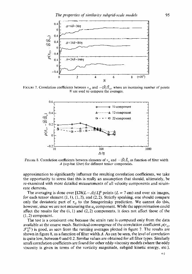
FIGURE 7. Correlation coefficients between T~~ and -If1 flz, where an increasing number of points N are used to compute the averages.

0.6 I I I

i C> 0.4 '3

- A. . . . . . . . . . . .A

D - - - !I

1 1-component 1 12-component

22-component

FIGURE 8. Correlation coefficients between elements of T~~ and - I$[ ftj as function of filter width A (top-hat filter) for different tensor components.

approximation to significantly influence the resulting correlation coefficients, we take the opportunity to stress that this is really an assumption that should, ultimately, be re-examined with more detailed measurements of all velocity components and strain- rate elements.

The averaging is done over [128(L-A)/Ll2 points ( L = 7 cm) and over six images, for each tensor element (1, l), (1,2), and (2,2). Strictly speaking, one should compare only the deviatoric part of 7ij to the Smagorinsky prediction. We cannot do this, however, since we are not measuring the us component. While the approximation could affect the results for the (1,l) and (2,2) components, it does not affect those of the (1,2) component.

The test is a consistent one because the strain rate is computed only from the data available at the coarse mesh. Statistical convergence of the correlation coefficient p(7ii, S$)) is good, as seen from the running averages plotted in figure 7. The results are shown in figure 8, as a function of filter width A . As can be seen, the level of correlation is quite low, between 0 and 0.2. Similar values are obtained for all filter types. Similarly small correlation coefficients are found for other eddy-viscosity models (where the eddy viscosity is given in terms of the vorticity magnitude, subgrid kinetic energy, etc.),

4-2

96 S. Liu. C. Meneveau and J . Katz

0.2 7~ I

> -0.2 - 1 1 -component

A- - - .. . t. ..-.A 12-component h W

Q

-0.4 [ D - - - 43 22-component

1 100 1000

-0.6 L . . . . . . . I 10

A 177 FIGURE 9. Correlation coefficients between elements of 7ij and the resolved vorticity component

G3, as function of filter width A (top-hat filter).

essentially because there is no alignment between the tensors T~~ and $6j in the first place. These results are entirely consistent with numerous previous findings based on DNS data, only that now they are confirmed for turbulence at considerably higher Reynolds number.

For completeness, we also present correlation coefficients between T~~ and the resolved vorticity component in the x3 direction. The results are shown in figure 9. As can be seen, the correlation is also low, not exceeding 0.2 in magnitude except at the largest scale. However, one should not conclude that vorticity is unimportant, since in $7, we shall find other more detailed relationships between stresses and the entire velocity gradient tensor, which includes the vorticity.

The results of this section serve as motivation to search for improved SGS modelling, that hopefully should display better agreement with the real stress. A starting point for this search is to observe the rate at which the real stresses dissipate resolved kinetic energy and how this energy flux is distributed amongst the small scales. The next two sub-sections focus on these questions.

4.5. Energy flux to subgrid scales The energy flux to unresolved scales is defined as follows: -

Lyd) = - T i j s,,, (22)

and one expects its (ensemble) average to be of the same order of magnitude as the dissipation rate t: in this near-equilibrium flow. To ascertain if this is the case for the present data, we compute the average of IZ(4) over the six images (i.e. a combination of spatial and ensemble averaging), for a range of filter sizes A . Since not all tensor elements entering the contraction on the right-hand side of (22) are being measured, some approximations must be made. In particular, we assume that ( T ~ ~ $ ~ ~ ) = ( T ~ ~ gZ3) = (-rI2 g12) and that ( T ~ ~ g33) = (;(T,, + T ~ ~ ) g3;,,). After using the incompressi- bility condition to evaluate &3 one obtains

While this expression would be exact for isotropic turbulence, we have found that isotropy conditions are not met among the terms that we can measure. However, since we shall focus on trends and not on exact numerical values of the energy flux, we proceed with our present approximations.


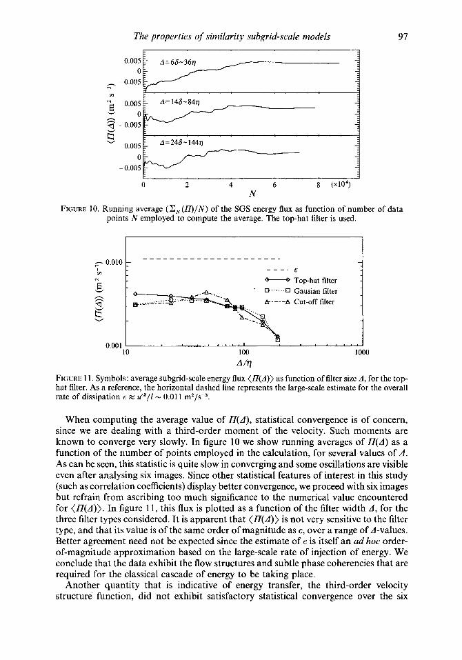
FIGURE 10. Running average (C, (ZZ)/N) of the SGS energy flux as function of number of data points N employed to compute the average. The top-hat filter is used.

- - - - _ _ _ _ _ _ - - - - - - - - - - - E

b--f, Top-hat filter Gausian filter Cut-off filter

n 0.010 “i

v)

N d

0.001 1 10 100

A 177 FIGURE 1 1 . Symbols: average subgrid-scale energy flux (ZZ(A)) as function of filter size A , for the top- hat filter. As a reference, the horizontal dashed line represents the large-scale estimate for the overall rate of dissipation E zz d 3 / l - 0.01 1 m2/s-3.

When computing the average value of n(A), statistical convergence is of concern, since we are dealing with a third-order moment of the velocity. Such moments are known to converge very slowly. In figure 10 we show running averages of n(A) as a function of the number of points employed in the calculation, for several values of A . As can be seen, this statistic is quite slow in converging and some oscillations are visible even after analysing six images. Since other statistical features of interest in this study (such as correlation coefficients) display better convergence, we proceed with six images but refrain from ascribing too much significance to the numerical value encountered for (n(A)). In figure 11, this flux is plotted as a function of the filter width A , for the three filter types considered. It is apparent that (n(A)) is not very sensitive to the filter type, and that its value is of the same order of magnitude as E , over a range of A-values. Better agreement need not be expected since the estimate of c is itself an ad hoc order- of-magnitude approximation based on the large-scale rate of injection of energy. We conclude that the data exhibit the flow structures and subtle phase coherencies that are required for the classical cascade of energy to be taking place.

Another quantity that is indicative of energy transfer, the third-order velocity structure function, did not exhibit satisfactory statistical convergence over the six

98 S . Liu, C. Meneveau and J . Katz

6

6

FIGURE 12. Contogr plots of spatial distribution of energy flux, for the top-hat fi1ter.i~) The ('not- so-local') flux T,, Sp,, going from scales above 24 to all scales smaller than A . (b) L,, S,,, the ' local' flux of energy that goes from scales larger than 2 4 to scales between A and 24. Darkest grey corresponds to a value of 0.0411 m2 ss3, and the contours are spaced by constant increments of -0.006 m2 s - ~ . White regions denote negative values.

images. More data will have to be analysed in order to obtain that variable reliably. On the other hand, the velocity-derivative skewness cannot be evaluated from these data since the dissipation range is not resolved.

4.6. Energyjux at a larger scale As a next step, we wish to study the flux of energy that goes to all scales smaller than 24. We use a definition slightly different from that of Z7(A), namely a consistent definition as far as LES on a grid with mesh size A is concerned. We define this flux as

(24)

(25) where 17*(2A) = - Tpq gp4, -

T . = u y - z . z . . 23 2 3 a ?

Here the overbar variables are computed based only on the tilde variables at the discrete A-mesh points, as discussed in $4.2.

Next, we recall the Germano identity (Germano 1992) and recognize that Z7*(2A) consists of two contributions,

L7*(2d) = - (Lpq zpq + Tpq gpq,. The resolved stress L, is defined as

- L. . = u".u".-z.z.

23 2 3 a 3'

1.0 1

h

0.8 1 - :: s It 2

0.6 - W

Q

1 0.4

99

and it will later be found to have substantial significance. The first term L,, Zpq can be interpreted as the energy flux from large scales to scales of sizes in bet_ween d and 26 (we shall refer to it as the ‘local’ contribution). The second term T,,$~, corresponds to the energy flux to scales smaller than d (referred to as ‘not-so-local’ contribution, because the scale disparity is larger than a factor of two).

In order to evaluate the two flux contributions from the data, we employ the approximations of (23), but without the averaging. It must be recognized that the present approximation is less justified than that of (23), since it is now invoked for the instantaneous values. We must postulate that the overall trends that are observed are not hfluenced too strongly by this approximation. Figure 12 shows contour plots of Lp,3p, and of T,,$?,. for the top-hat filter and for d = 86 - 4811. At each point, the sum of both quantities yields Z7*(2d). According to the discussion in $4.2, these variables are defined on a coarser grid ([xl], + 2j1 A , [x,], + 2jz A ] . Nevertheless, a smooth field can be obtained (for plotting purposes) by sliding the reference point ([x,],,, [x,],) inside the initial coarse box, centred at ( j , = O , j , = 0).

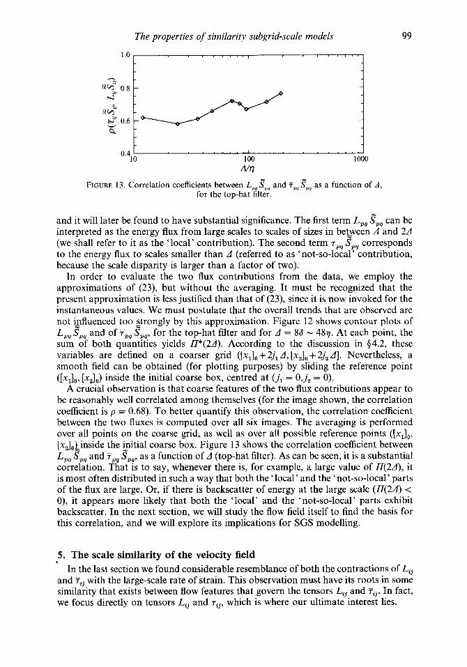
A crucial observation is that coarse features of the two flux contributions appear to be reasonably well correlated among themselves (for the image shown, the correlation coefficient is p = 0.68). To better quantify this observation, the correlation coefficient between the two fluxes is computed over all six images. The averaging is performed over all points on the coarse grid, as well as over all possible reference points ([xJ0, [x,],Linside the Lnitial coarse box. Figure 13 shows the correlation coefficient between L,, S,, and T,, sppq, as a function of d (top-hat filter). As can be seen, it is a substantial correlation. That is to say, whenever there is, for example, a large value of Z7(24), it is most often distributed in such a way that both the ‘local’ and the ‘not-so-local’ parts of the flux are large. Or, if there is backscatter of energy at the large scale (Z7(2d) < 0), it appears more likely that both the ‘local’ and the ‘not-so-local’ parts exhibit backscatter. In the next section, we will study the flow field itself to find the basis for this correlation, and we will explore its implications for SGS modelling.

5. The scale similarity of the velocity field In the last section we found considerable resemblance of both the contractions of Lii

and Tij with the large-scale rate of strain. This observation must have its roots in some similarity that exists between flow features that govern the tensors Lii and Tii. In fact, we focus directly on tensors Lii and 7ii, which is where our ultimate interest lies.

4


5.0

4.5

4.0

3.5 3.5 4.0 4.5 5.0 3.5 4.0 4.5 5.0 3.5 4.0 4.5 5.0

XI (cm) XI (cm) X I (cm) FIGURE 14. Velocity maps in consecutive bands, of characteristic scale L/2" (where L = size of entire image). From ( a H c ) : n = 3,4,5. The bands are defined as the difference between two low-pass- filtered versions of the velocity field. Larger-scale fields are sampled on coarser grids that properly emulate the information available during LES. Bilinear interpolation is used to generate smooth fields, for graphical purposes. To avoid crowding, only a subset of an image is shown. Some similar features in vortical regions can be recognized in consecutive bands.

5.1. The velocity jield decomposed into bands It is useful to separate the data into different scales of motion ('bands'). This decomposition facilitates the identification of flow features that dominate events close to the cut-off A of interest. We now decompose the fluctuating velocity field ui(x) into contributions from separate bands, according to

where the velocity field in each band is given by

u!"'(x) = tl,(x) - @<(X). (29)

The tilde represents top-hat filtering at a scale A = 2-"L while the overbar also represents low-pass filtering, but at a larger scale 2-("-l)L. However, in order to assure that no trivial overlap of information between bands is generated, we must again be careful how these data are sampled. For the tilde operation we use sampling on a grid of size A . Then some known (e.g. bilinear) interpolation scheme is employed to generate a 'smooth' field in between those points, for graphical illustration purposes. The overbar operation only uses information that is available on the A-grid and is itself sampled on a grid of spacing 24 = 2-("-')L. Again, a smooth field is generated by (bilinear) interpolation. The: band-velocity ul")(x) is the difference between the two smooth fields, each of which has been constructed only with discrete information available at the previous step.

5.2. The scale coherence ofpow structures From our data set, we consider three bands ranging from n = 3 to n = 5 (while N = 7). Figure 14 shows samples of the vector fields a:"). For clarity, only small subsets of the entire vector fields are shown. If we focus attention on the highlighted regions, we notice some similarity between (sections of) vortex-like flow structures that exist in consecutive bands, at about the same locations. Some streaming regions also display similarity. We have made similar observations based on the other images. Of course, the similarity does not extend to the entire flow field, as the smaller-scale bands contain


more structures with no counterparts at the large scales. For instance, the lower-right corners in the vector maps for n = 3 and n = 4 (figure 15) exhibit distinctly different flow features.

Two physical interpretations for this partial scale coherence can be ventured. The first involves the concept of the energy cascade, in the following sense : small eddies (in band n + 1) have some history in common with the larger eddies (in band n). They have both been influenced by the even bigger eddies (from band n- l), during some time interval. Although by classical arguments one expects that the strongest influence on band n + 1 comes from band n, some influence from band (n - 1) is still felt by band n+ 1 ('not-so-local' interactions). Thus the 'effective forcing' of bands n and n + 1 due to band n - 1 has some degree of similarity. Therefore, it is plausible that their response (the resulting velocity field) may also show some common features. A second interpretation can be given in terms of coherent structures: clearly, a physically meaningful flow structure needs information from several bands (unless one defines the bands using a filter which is exactly parallel (in function space) to the structure itself). If a given structure is decomposed into bands, the correlation may arise because one is really looking at the same single structure. Both interpretations may in fact be related, or complementary. For now, we use the observations for modelling purposes.

5.3. Relation between SGS stress and velocity bands Now that we have qualitatively shown some resemblance between the velocities in successive bands, a connection must be found between them and the SGS stress 7ii.

Using the usual scaling arguments one can argue that the SGS stress is dominated by the largest unresolved scales. In other words, if we select d = 2FL, then 7ii should be dominated by uin+l). This argument is not complete, however, owing to the known large-scale contribution to the SGS stress which appears through the Leonard stress and the cross-stress (Leonard 1974). Therefore, to approximate the SGS stress one should at least keep the last resolved band (n) and the first unresolved one (n+ 1) as follows:

_I _I

A h A

7:;) = ~u,"+u,"+~)(u;+u;+~j-~(u:+u,"+~)"(u;+u;+').' (30)

The tilde represents, as before, filtering at scale d of the entire expression contained below the bracket. Figure 15 shows contour plots of the band-approximated stress element 7i;)(x) and the real stress ~ ~ ~ ( x ) , for A = Y 3 L (n = 3). The latter variable has been constructed in a similar way : by sampling on a grid of mesh size d coincident with the grid used to generate 7g)(x), and using bilinear interpolation. As can be seen, the representation in terms of two bands surrounding the cut-off scale is quite satisfactory. The correlation coefficient between each element 7i;) and 7ii is typically close to 0.83.

As a parenthetical disgression, we remark that (30) can be written as

where

is akin to a SGS Reynolds stress which involves only the small scales, rs_ -- - _ - g;) = (u;" u; - u;+1 uj") + (u; ,;+1 - u; Uj"+l)

cz_ d- is a cross-stress, while

,y!?) = U n un - Un ut v 1 3 2 3

resembles a Leonard stress involving solely the resolved scales. Each of these expressions is Galilean invariant, as opposed to the definitions usually employed, for

102 S. Liu. C. Meneveau and J. Katz

FIGURE 15. (a) Contour plot of the real SGS stress element 712, computed with a top-hat filter of width d = 2-3L. Contours range from -0.0048 m2 s - ~ (dark) to 0.00288 m2 ss2, at intervals of 0.00096 m2 s-~. (b) Contour plot of 7g), the SGS stress estimated from the velocity field in the two bands surrounding the scale A . Contours range from -0.002 m2 s - ~ (dark) to 0.002 m2 ss2, at intervals of 0.0005 me s-'.

which the cross-stresses do not have this property. In this regard these expressions mirror the elegant decomposition proposed some time ago by German0 (1986).

6. The stress-similarity model The basic observation of similarity between the vector fields uin+') and uln) (and

between uin) and uln-l)) means that there is some similarity between 7;;) and 7;y-1). We have already shown that 7:;) is a good approximation for the real SGS stress rij . A further approximation that simplifies the formulation is to rewrite 717-l) in terms of the band velocities, and use (29). One obtains

(32)

where the hat signifies further filtering of the overbar data at a scale 44 = 2-(n-2)L. Since __ zi is almost constant over distances of 24, we can approximate products involving tii as Ci zij M Gi Gj. It leads to a cancellation of Ci and yields T~Y-') M Lii. Finally, these considerations imply that there must be some similarity between rij and Lij. If no better information is available, it would appear that a 'best guess' for the SGS stress is to set it to be proportional to L,. Finally, the proposed stress-similarity model reads

_ _ _ ~ Ti;-'' = (Ci - zi i ) (Ci - zit) - (iii - tii) (Cj - Gj),

Ki = C L L,. (33)


The stress Lii can be entirely computed from the resolved velocity at the LES grid points; cL is a dimensionless model coefficient yet to be specified (see 99).

A comparison among 712, L,, and the Smagorinsky prediction 9it) = - 2(c, A ) , Is”] g,, is presented by the colour contour maps in figure 16. As explained before, we have computed 712 at points x, while computing L,, and gii by only employing the (discrete) data iii(xl +md , x, + nd). However, a smooth contour plot is produced by varying x along the original fine mesh. The vector maps represent the velocity fields on which these tensors depend most strongly, namely the fields in bands n = 4 and n = 3, respectively. The filter size is d = 86 - 487 and a top-hat filter has been used. It is evident that the agreement between 7,, and the stress-similarity model is significantly better than between 7,, and the Smagorinsky model. One important distinction between L,, and 7,, is that the fluctuations of L,, occur over bigger lengthscales than those of 7,,. This discrepancy is due to the fact that the former is dominated by the unresolved scales of motion (shown by the vectors in figure 16a), while those of L, are dominated by the resolved velocity field zdn) (shown by the vectors in figures 16b and 16c). The similarity between the vector fields zdn+l) and u(”) described before can be also observed here.

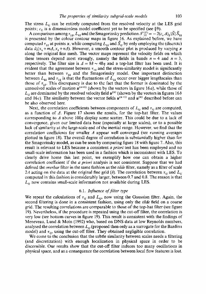
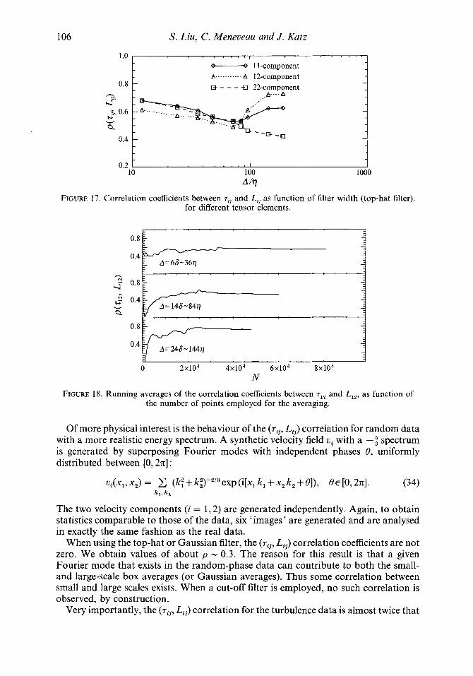
Next, the correlation coefficients between components of L, and 7ii are computed, as a function of A . Figure 17 shows the results, for the top-hat filter. The values corresponding to d above 1007 display some scatter. This could be due to a lack of convergence, given our limited data base (especially at large scales), or to a possible lack of similarity at the large-scale end of the inertial range. However, we find that the correlation coefficients for smaller d appear well converged (see running averages plotted in figure 18). The overall degree of correlation is substantially higher than for the Smagorinsky model, as can be seen by comparing figure 18 with figure 7. Also, this result is relevant to LES because a consistent a priori test has been employed and no small-scale information has been used in a fashion which is inconsistent with LES. To clearly drive home this last point, we exemplify how one can obtain a higher correlation coefficient if the a priori analysis is not consistent. Suppose that we had defined the overbar filter in the same fashion as the tilde filter, namely as a filter of scale 24 acting on the data at the original fine grid (6). The correlation between 7ii and Lii computed in this fashion is considerably larger, between 0.7 and 0.8. The reason is that Lii now contains small-scale information not available during LES.

6.1. Influence of filter type We repeat the calculations of 7ij and L,,, now using the Gaussian filter. Again, the second filtering is done in a consistent fashion, using only the tilde field on a coarse grid. The resulting correlations are comparable to those of the top-hat filter (see figure 19). Nevertheless, if the procedure is repeated using the cut-off filter, the correlation is very low (see bottom curves in figure 19). This result is consistent with the findings of Meneveau, Lund & Moin (1992) who, based on DNS data at low Reynolds numbers, analysed the correlation between Lij (proposed then only as a surrogate for the Bardina model) and rii, using the cut-off filter. They obtained negligible correlation.

We come to the conclusion that the subtle similarity between scales needs a filtering (and discretization) with enough localization in physical space in order to be discernible. Our results show that the cut-off filter induces too many oscillations in physical space, and as a consequence the correlation between local flow features is lost.


FIGURE 16. For caption see facing page.

The properties of similarity subgrid-scale models

6.2. Comparison with the Bardina model As outlined in the introduction, the first similarity model was proposed by Bardina et al. (1980). It involves a second filtering at the grid-level scale A , as opposed to the scale 24 used to calculate L,. We have repeated the consistent a priori test for the Bardina model. Usually, the Bardina model is used in conjunction with the Gaussian filter, which puts some weighting on all points of the 4-grid. However, we notice that the weights of even the closest points are very small compared to the central point (their ratio is exp (6) - 400!). The consequence is that the fluctuations of S$?) are very weak. We have measured the r.m.s. level of rij and that of Sf) from the data, at A = 146. We find the former to be cr7 - 1.4 x m2 s-'. This disparity in intensity means that the model has little influence on the simulation, unless it is multiplied by a very large model coefficient. On the other hand, the low- intensity fluctuations of s::) do display some similarity with those of rii. The corresponding correlation coefficients are only marginally lower k ( ~ ~ ~ , s:,")) m 0 .54 .55 ) than those of Lij. We may point out that in the past (Bardina et al. 1980, etc.), this model was reported to have much higher correlation (p - 0.8). We have repeated the a priori test in the traditional fashion, i.e. with a second filtering based on the fine- grained data (where Gi is employed at all grid points of the 8-mesh when computing the second filtering). Then the result is p - 0.85, which is quite comparable to the earlier results based on DNS a priori testing. However, we argue that such a high correlation is an artifact of using information that is unavailable during LES.

In spite of this 'critique' of the initial formulation of the similarity model, it is highly encouraging to find that the correlation of the revised model is still substantially higher than that of the Smagorinsky model. The basic physical ideas that underlie the approach originally proposed by Bardina et al. (1980) appear hereby corroborated from the consistent a priori test applied to the experimental data.

6.3. Analysis of synthetic fields Another question which, for completeness, we would like to address is the following: What correlations are obtained when analysing random, non-turbulent fields? With such a question we mean to verify that the correlations observed between rij and Lij are a result of physical processes and not some artifact which may be valid for any type of signals. For this purpose, we generated velocity fields consisting of random numbers (white noise). Each velocity component is generated independently, and a total of six 'images' consisting of 128 x 128 random vectors are considered. One would not expect to find correlations between rij and L, for this type of data. In fact, one obtains values that are almost zero (see figure 20 where a running average is presented, for A = 146 and a top-hat filter). The slight deviation from zero is because statistical convergence is not complete.

105

m2 s-', while the second is crB - 6 x

FIGURE 16. (a) Contour plot of the real SGS stress element T,, computed with a top-hat filter. The filter size is in the inertial range ( A = 86 - 489; 6 = measurement grid size, 9 = Kolmogorov scale). Contour levels range from dark blue ( T ~ , = -4.8 x mz s-,), in increments of 0.64 x m2 s-,. The vectors represent the largest of the 'unresolved' velocity field u("+l). A vector length of 1 cm (in units of the figure) corresponds to a velocity of 0.22 m s-'. (b) Contour plot of L,,, the stress computed based on the resolved velocity field. For a discussion on the consistent sampling procedure used, see text. Contour levels range from dark blue (L12 = -3.2 x m2 s - ~ . The vectors represent the-scaliest scales of the resolved velocity field, u(') (same units as in (a)). (c) Contour plot of F& = - IS1 S,,, the prediction of the Smagorinsky model (without the model constants). Contour levels range from dark blue (Ss, = - 1025 s - ~ ) to red (SS, = 3 5 5 s?), in increments of 110 s-'. As above, the vectors represent u(") which contributes mostly to S,.

m2 s-,) to red ( T ~ ~ = 2.9 x

m2 s - ~ ) to red (Liz = 2.7 x m2 s - ~ ) , in increments of 0.5 x

106

1 .o I - 1 1-component A.- - - - -....- A 12-component D - - - +I 22-component

&...A

- 0.8 - % 4 - :S 0.6 . _____ c. U

Q

0.4 - -

0.2 I

S. Liu, C. Meneveau and J. Katz

0.8

1 0.4

0.8

0.4

0'4 ""I(--- A=24S- 144q Fl 0 2x104 4x104 6x104 8x104

N

FIGURE 18. Running averages of the correlation coefficients between T~~ and L,,, as function of the number of points employed for the averaging.

Of more physical interest is the behaviour of the (7ij, L!?) correlation for random data with a more realistic energy spectrum. A synthetic velocity field vi with a --: spectrum is generated by superposing Fourier modes with independent phases 0, uniformly distributed between [0,27c] :

(34) ui(xl, xz) = (k,2 + ki)-z/3 exp (i[xl k , + x2 k , + el), B E [0,27c]. k , , k ,

The two velocity components (i = 1,2) are generated independently. Again, to obtain statistics comparable to those of the data, six 'images' are generated and are analysed in exactly the same fashion as the real data.

When using the top-hat or Gaussian filter, the (7ij, Lij) correlation coefficients are not zero. We obtain values of about p - 0.3. The reason for this result is that a given Fourier mode that exists in the random-phase data can contribute to both the small- and large-scale box averages (or Gaussian averages). Thus some correlation between small and large scales exists. When a cut-off filter is employed, no such correlation is observed, by construction.

Very importantly, the (7ii, Lij) correlation for the turbulence data is almost twice that

1 .o 1

0.8 - +-+ I 1 A. .A A-A 12

D fl 22

Gausian filter: -

- n

n 4> +> 0.4 - Q Cut-off filter:

- v

107

-0.2 t I

10 100 1000 A h

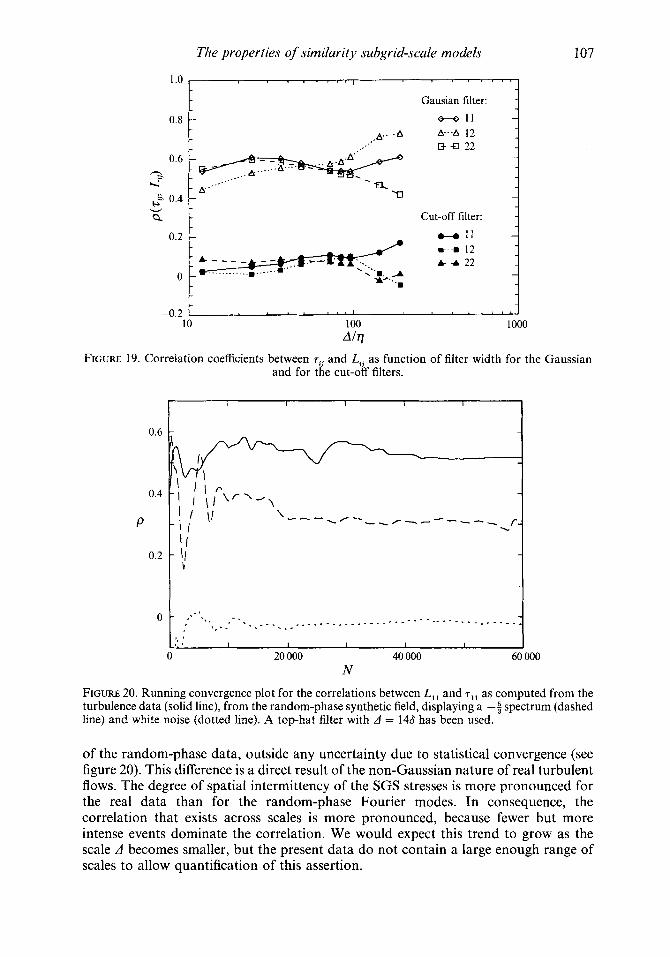
FIGURE 19. Correlation coefficients between T~~ and Ltj as function of filter width for the Gaussian and for the cut-off filters.

0.6

0.4

P

0.2

0

N

FIGURE 20. Running convergence plot for the correlations between L,, and T , ~ as computed from the turbulence data (solid line), from the random-phase synthetic field, displaying a -$ spectrum (dashed line) and white noise (dotted line). A top-hat filter with A = 148 has been used.

of the random-phase data, outside any uncertainty due to statistical convergence (see figure 20). This difference is a direct result of the non-Gaussian nature of real turbulent flows. The degree of spatial intermittency of the SGS stresses is more pronounced for the real data than for the random-phase Fourier modes. In consequence, the correlation that exists across scales is more pronounced, because fewer but more intense events dominate the correlation. We would expect this trend to grow as the scale d becomes smaller, but the present data do not contain a large enough range of scales to allow quantification of this assertion.


Thus, the scale coherence manifested in the (rii, L,) correlation has a 'kinematic' component (due to spectral characteristics) which is present even in random-phase data, and a 'dynamic' component (due to spatial intermittency) which a random-phase signal does not possess.

6.4. Comparison at the vector level In this section we compare the divergence of the real and modelled stresses. The divergence is approximated as follows :

As required by measurement limitations, we cannot include the third term representing the effect of the velocity fluctuations normal to the image. We have computed the correlation coefficients between the elements of V . 7 and V - L using the above approximations. The results are typically close to p - 0.4, i.e. 30 % lower than for the tensor elements themselves. A possible cause for the difference in correlation coefficients is the mismatch in characteristic lengthscales between the fields rij and Lii. The corresponding correlation coefficients for the divergence of the Smagorinsky model, however, are still much lower ('p < 0.2). A more systematic study of the SGS stress divergence is left as future task to be undertaken once more complete (three- dimensional) experimental data become available (see concluding remarks in § 10).

7. Relation between stresses and the velocity gradient tensor: the nonlinear model

For the purpose of establishing a relationship between Lij and nonlinear SGS models, let us approximate the velocity field Ci as a piecewise-linear vector field in the neighbourhood of each point on the A-mesh. Similar arguments have been employed before to estimate the Leonard and cross-stresses (Leonard 1974; Clark et al. 1979; Horiuti 1993). Let us denote some given point of the A-mesh by xo. The procedure will be to evaluate L, by a top-hat filtering applied to the assumed linear velocity field around xo.

By expanding iii in Taylor series around xo we can write

Ci(X) = Ci(X0) + 'Xik(X0) (Xk - x;) + . . . . (36)

Nevertheless, we argue that this approximation is, in fact, not very good. The reason is that the linearized field, once filtered by the top-hat filter, produces a mean value equal to iii(xo), which is different from the real 'local average' Zi:

This defect can easily be remedied by using, instead of Ci(xo), the real average velocity as reference velocity, yielding

With this more realistic approximation for Ci(x) in the neighbourhood of xo, one can now evaluate the expression for Lii. The result is the following:

Lij(X0) % ~AZ&(XO) A",,(XO). (39)


“ 0

6

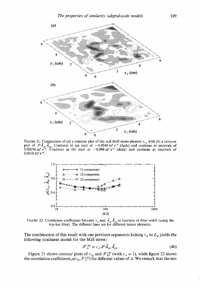
FIGURE 21. _Cornparison of (a) a contour plot of the real SGS stress element T~~ with (b) a contour plot of d2A,,A, , . Contours in (a) start at -0.0048 m2 s-’ (dark) and continue at intervals of 0.00096 m2 s-’. Contours in (b) start at -0.008 m2 s? (dark) and continue at intervals of 0.0018 m2 ss2.

1.0, I I (t----o 1 1-component A--.- - - ------A 12-component

..A

- ..... A c. W Q 0.6

t 0.4 I I I

10 100 1000

A177 FIGURE 22. Correlation coefficients between rij and itk ijF as function of filter width (using the

top-hat filter). The different lines are for different tensor elements.

The combination of this result with our previous arguments linking 7ii to L, yields the following nonlinear model for the SGS stress:

w -

F j f ) = cA A2A, Ajk. (40) Figure 21 shows contour plots of 712 and 9-g) (with cA = I), while figure 22 shows

the correlation coefficients p(7ii, Sij”)) for different values of A. We remark that the test


is a consistent one, because A”ij has been evaluated from the data at the A-grid level. As can be seen, the correlation is comparable to that observed in the L, formulation. However, we shall argue later that the model in terms of Lij is preferable to the velocity-gradient formulation. The reason will be clear when we consider the near-wall behaviour in 99.

Note that if the spectral cut-off filter is employed, the correlation between rij and S$‘) is much weaker @ - 0.2). This may explain the previously negative findings of Meneveau et al. (1992) and Lund & Novikov (1992). They tried, using cut-off filtering of low-Reynolds-number DNS data, to correlate the SGS stresses with a variety of combinations of the velocity gradients. For isotropic turbulence, no strong correlations were found, which is also consistent with the low correlation for the similarity model L,, using the cut-off filter. However, for shear flows there was considerable indication of nonlinear dependencies between rij and the resolved velocity gradients, even when using the cut-off filter. These trends remain to be explained. In addition, we point out that Horiuti (1993) has proposed a nonlinear model which contains, as one of its many terms, an expression equivalent to S!;).

Finally, it is pertinent to comment on the cause for the violation of material-frame indifference in (40). In general, such a violation is not unexpected for turbulent flows (Lumley 1970). For the present model, its origin lies in the fact that the real stress depends on the vorticity of the unresolved velocity field. This vorticity is then linked to the resolved vorticity through the similarity modelling. One expects the spectral closeness of the turbulence interactions to preclude the separation of scales that is required for the appearance of frame-invariant constitutive relations. This feature is explicitly taken into account in the similarity model.

8. Energy dissipation and backscatter control

are computed according to Figure 23 shows contour maps of the real and modelled local SGS energy flux. These

w w

LT, = - rij Sij and LT, = - L, S,. (41) The tensor contractions have been approximated in terms of the measured elements in the same fashion as (23). The fact that both fields exhibit some coarse resemblance is due to the considerable correlation that exists between rij and Lij. Significant portions of the flow where backscatter exists (I7 < 0) appear in both the ‘real’ and ‘modelled’ fields of energy flux. From these results it may appear that the modelling based on Lij can capture backscatter in a reasonable manner. However, as outlined in 9 1, experience from LES calculations with similarity models (see e.g. Bardina et al. 1980) shows that calculations become unstable because such models are not dissipative enough. The remedy has been to add a term of the eddy-viscosity type, yielding ‘mixed models’ (Bardina ef al. 1980; Horiuti 1993, etc.). We have tested the following version of the mixed model:

STix = - 2(c, A)2 Is”( gtj + cL L,,.

We have chosen the Smagorinsky coefficient in the usually employed range c, = 0.1 to 0.2. Since we found the level of fluctuations of L, to be of the same order of magnitude as those of rii, we set cL = 1. Interestingly, the correlation coefficients between rij and Fzix that are measured from our data sets are essentially the same as those of the stress-similarity model alone. The main reason is that the typical magnitudes of the Smagorinsky term are much smaller than those of L,,, and thus do not affect its correlation with the real stress (for a more detailed discussion, see Liu, Meneveau &


6

FIGURE 23, Contour plots of SGS energy flux. (a) The flux estimated_ from the real SGS stress, Z7, = - 71j Sij . (b) The SGS flux implied by the modelled stress nL = - L, St,. Darkest grey corresponds to a maximum value of 0.0288 m2 ss3, and the contours are spaced by constant increments of - 0.0036 m2 s@. White regions denote negative values.

Katz 1994a). However, since the Smagorinsky term is well correlated with the resolved strain rate, it systematically contributes to positive dissipation of energy. From this point of view, such a mixed model appears to be a very desirable option (see Zang, Street & Koseff 1993 and Akhavan, Ansari & Mangiavacci 1993 for recent numerical work using mixed models).

In $9 we shall discuss some difficulties that occur near solid walls when adding eddy- viscosity terms. Therefore, it is useful to suggest a possible alternative which consists in selectively weighting the similarity stress with the amount of energy dissipation that it is generating. The SGS dissipation depends on the alignment between the two tensors Lij and ITij, which can be quantified by the following dimensionless invariant :

One can show that ILS is bounded between - 1 and 1. We now postulate a similarity model in which there is some dependence on the strain-rate tensor, through the following formulation :

HereAZLS) is a dimensionless scalar function which depends on ZLs. If we choose

q y ) = CLAZLS) Lij. (44)

M L S ) = I L S , (45)

112 S. Liu, C. Meneveau and J. Katz

0.6 I

10 100

A h 1000

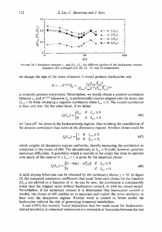
FIGURE 24. Correlation between T~~ and j(lLs) Ltl, for different choices of the backscatter control functionsfll) averaged over the 11-, 12- and 22-components.

we change the sign of the stress whenever it would generate backscatter and

is evidently positive everywhere. Nevertheless, we would obtain a positive correlation between 7ii and F--(fL) whenever L, is preferentially counter-aligned with the strain rate ( ILs > 0) while obtaining a negative correlation when ILs < 0. The overall correlation is thus very low. On the other hand, if we define

we ‘turn off’ the stress in the backscattering regions, thus avoiding the cancellation of the positive correlation that exists in the dissipative regions. Another choice could be

1 if ILs >, 0 0 if ILs < 0, (47)

which weights all dissipative regions uniformly, thereby increasing the correlation as compared to the choice of (46). The discontinuity at ILs = 0 could, however, generate numerical difficulties. A possibility which is smooth at the origin but close to uniform over much of the interval 0 < ILs < 1 is given by the empirical choice

A mild sloping behaviour can be obtained by the (arbitrary) choice y = 10. In figure 24, the measured correlation coefficients that result from each choice for the function f l ILs ) are plotted as a function of A . As can be seen, the correlation is considerably lower than the original value without backscatter control, or with the mixed model. Nevertheless, if for numerical reasons it is determined that backscatter control is needed, the choice of (48) enables us to maintain and exploit the stress similarity at least over the dissipative regions. Further work is needed to better model the backscatter without the risk of generating numerical instabilities.

Lund (1993) has recently found indications that the main cause for backscatter- related instability in numerical simulations is a mismatch of timescales between the real

0.8

0.6

C L 0.4

0.2

113

I

- . - - e 0 -. ------,-*----=--------- - -

0 . 3 0

- -

I

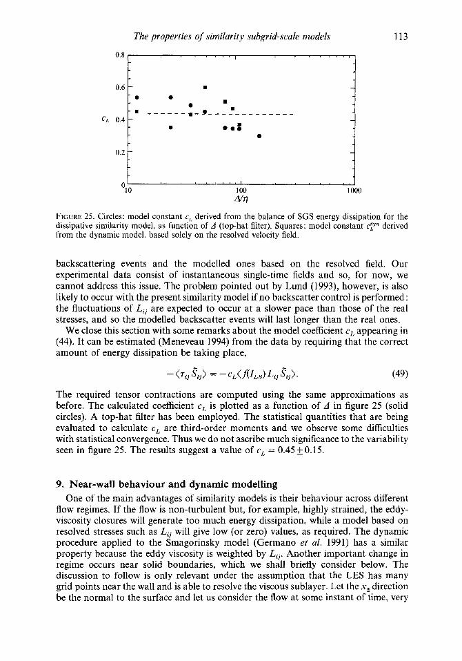
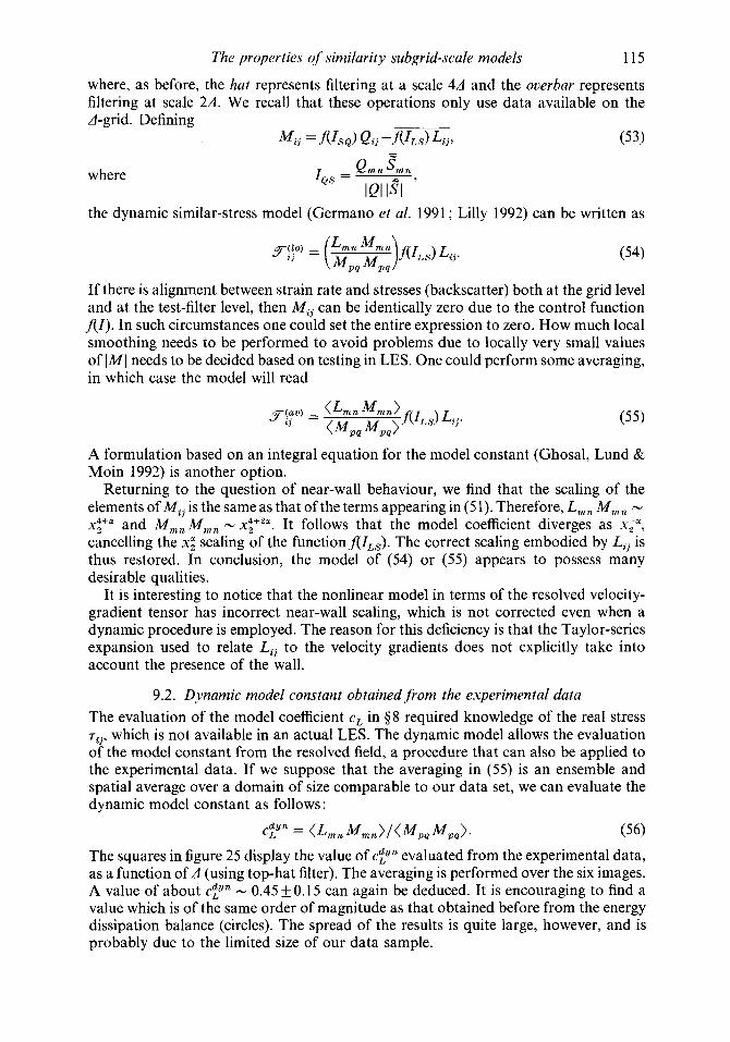
FIGURE 25. Circles: model constant c, derived from the balance of SGS energy dissipation for the dissipative similarity model, as function of A (top-hat filter). Squares: model constant c y derived from the dynamic model, based solely on the resolved velocity field.

backscattering events and the modelled ones based on the resolved field. Our experimental data consist of instantaneous single-time fields and so, for now, we cannot address this issue. The problem pointed out by Lund (1993), however, is also likely to occur with the present similarity model if no backscatter control is performed : the fluctuations of Lij are expected to occur at a slower pace than those of the real stresses, and so the modelled backscatter events will last longer than the real ones.

We close this section with some remarks about the model coefficient cL appearing in (44). It can be estimated (Meneveau 1994) from the data by requiring that the correct amount of energy dissipation be taking place,

The required tensor contractions are computed using the same approximations as before. The calculated coefficient cL is plotted as a function of d in figure 25 (solid circles). A top-hat filter has been employed. The statistical quantities that are being evaluated to calculate cL are third-order moments and we observe some difficulties with statistical convergence. Thus we do not ascribe much significance to the variability seen in figure 25. The results suggest a value of cL = 0.45f0.15.

9. Near-wall behaviour and dynamic modelling One of the main advantages of similarity models is their behaviour across different

flow regimes. If the flow is non-turbulent but, for example, highly strained, the eddy- viscosity closures will generate too much energy dissipation, while a model based on resolved stresses such as L, will give low (or zero) values, as required. The dynamic procedure applied to the Smagorinsky model (German0 et al. 1991) has a similar property because the eddy viscosity is weighted by Lij. Another important change in regime occurs near solid boundaries, which we shall briefly consider below. The discussion to follow is only relevant under the assumption that the LES has many grid points near the wall and is able to resolve the viscous sublayer. Let the x2 direction be the normal to the surface and let us consider the flow at some instant of time, very


near the wall. We perform a Taylor series expansion at the wall of the instantaneous velocity field in the x2 direction. We find u, - x,, u, - x i and u, - x,. The near-wall scaling of the real instantaneous SGS stress tensor is therefore as follows:

Tll - xi, 722 - xi, r33 - xi, T12 - xi, T13 - xi, rz3 - xi.

If one defines the stress by subtracting its isotropic part, the result is identical except for rZ2 which now would scale like the other two normal stresses, rZ2 - xi. For the Smagorinsky model with no wall functions or dynamic model, the scaling with respect to x, is quite different than that of the real stresses. It is as follows:

g C S ) 11 x2, y ( S ) 22 - x2, y ( S ) 33 - x,, y!:) - const., F(’) 13 - x2, 9:;) - const.

A very desirable feature of the dynamic model

is that it can correct the behaviour of the most relevant term, T~~ (German0 et al. 1991 ; Piomelli 1993). Using the fact that the scaling of each element of Lij and Mij is the same as that of rij and Sij, respectively, one obtains the near-wall scalings L,, M,, - xi and M,, M,, - const. It follows that the dynamic Smagorinsky model scales (instan- taneously) as

F C S ) 11 - x;, - x;, 5:;) - x;, Yg) - x;, Fit) - x;, Fit) - x; near the wall. Therefore, only the r12 and rZ3 elements display the right behaviour. If the wall is a plane and the mean flow direction is xl, then on average rI2 is the only non- zero element. Its average value is needed for the calculation of the skin friction. However, if one is interested in predicting, for instance, the spectrum of wall-pressure fluctuations, it is easy to show that the subgrid-scale contributions arise from second- order moments of the SGS stress. Therefore, correct instantaneous scaling of the other tensor elements should also be desirable. For dynamic control purposes, realistic descriptions of individual realizations is also of importance.

Next we consider the proposed stress-similarity model, without backscatter control. It is obvious that each term displays the correct near-wall behaviour. However, as soon as we multiply Lij by a backscatter control functionfll,,), this property is upset: the scaling of L,,g,, is L,,gp, - xi and that of L,, L,, is - x:. Thus ZLs - xz as one approaches the wall. Suppose thatf(Z,,) - IFs near the origin (in the case of (48) we have a = 2). Then the near-wall behaviour of the model is

(51) ,I y ( f U - X2+a, y ( f U x4+a, y ( f U - x-+a y ( f L ) - x;+a, y ( f L ) - x;+a, y ( f L ) - x3+a,

11 2 22 2 33

12 13 23 2

which is clearly unsatisfactory. This erroneous near-wall behaviour can be fixed, as shown in the next section.

9.1. A dynamic stress-similarity model In order to evaluate the coefficient cL which appears in the similar-stress model and also to attempt to eliminate the previously found problem near solid walls, we apply the dynamic procedure to the present model. For this purpose we define a stress analogous to Lii but at twice the scale


where, as before, the hat represents filtering at a scale 44 and the overbar represents filtering at scale 24. We recall that these operations only use data available on the A-grid.- Defining

where

the dynamic similar-stress model (German0 et al. 1991 ; Lilly 1992) can be written as

If there is alignment between strain rate and stresses (backscatter) both at the grid level and at the test-filter level, then Mij can be identically zero due to the control function AZ). In such circumstances one could set the entire expression to zero. How much local smoothing needs to be performed to avoid problems due to locally very small values of [MI needs to be decided based on testing in LES. One could perform some averaging, in which case the model will read

A formulation based on an integral equation for the model constant (Ghosal, Lund & Moin 1992) is another option.

Returning to the question of near-wall behaviour, we find that the scaling of the elements of Mi, is the same as that of the terms appearing in (51). Therefore, L,, M,, N

x : + ~ and MmnMm, - x:+'~ . It follows that the model coefficient diverges as xia, cancelling the x; scaling of the functionAILS). The correct scaling embodied by Li, is thus restored. In conclusion, the model of (54) or (55) appears to possess many desirable qualities.

It is interesting to notice that the nonlinear model in terms of the resolved velocity- gradient tensor has incorrect near-wall scaling, which is not corrected even when a dynamic procedure is employed. The reason for this deficiency is that the Taylor-series expansion used to relate L,, to the velocity gradients does not explicitly take into account the presence of the wall.

9.2. Dynamic model constant obtained from the experimental data The evaluation of the model coefficient cL in $ 8 required knowledge of the real stress ri,, which is not available in an actual LES. The dynamic model allows the evaluation of the model constant from the resolved field, a procedure that can also be applied to the experimental data. If we suppose that the averaging in (55) is an ensemble and spatial average over a domain of size comparable to our data set, we can evaluate the dynamic model constant as follows :

(56) The squares in figure 25 display the value of ciyn evaluated from the experimental data, as a function of 4 (using top-hat filter). The averaging is performed over the six images. A value of about c p n - 0.45 f 0.15 can again be deduced. It is encouraging to find a value which is of the same order of magnitude as that obtained before from the energy dissipation balance (circles). The spread of the results is quite large, however, and is probably due to the limited size of our data sample.

p u n L = (Lmn M m n ) / ( M p q M p G ) .

116 S . Liu, C. Meneveau and J. Katz

10. Summary and conclusions Particle displacement velocimetry has been employed to measure a set of

instantaneous velocity vector maps in the far field of a turbulent round jet. The energy spectrum of the data was shown to match the Kolmogorov spectrum quite well, with over a decade of inertial range. By suitably filtering the data at inertial-range scales d(7 4 d < I ) , a priori analysis of several models for the turbulence subgrid stresses was performed. Since only two out of three velocity components were measured, some assumptions had to be made when evaluating tensor contractions. Also, since the data were obtained in a planar section of the flow, the filtering was done in two rather than three dimensions. These are the limitations of the present approach as compared to the analysis of DNS data. However, we were able to study a flow with realistic boundary conditions at a much higher Reynolds number (Rh - 310).

As a first step, the SGS stress field was measured and its properties were documented. Next, the correlation coefficients with the strain rate (as in the Smagorinsky model) were shown to be very small (p - 0.15), implying that locally the eddy-viscosity closures perform very poorly. While this finding is in agreement with numerous previous results from a priori analysis of DNS data, we have now been able to confirm them in a much higher Reynolds-number flow. Next, the measured SGS flux of kinetic energy was shown to be of the same order of magnitude as the overall energy dissipation u ‘ ~ / I - c. By examining spatial features of the flux of energy at a larger scale and how it is divided into ‘local’ and ‘not-so-local’ contributions, it became apparent that the flow fields in consecutive scales of motion must have some similarity.

For the rest of the paper the focus was on documenting this similarity in various ways, and on exploiting it in formulating a new similarity model. Some similarity was observed between the velocity fields in consecutive bands representing the motion of different scales. Care was taken not to use overlapping information that could artificially increase this similarity. A natural choice for a model was shown to be a self-similar rescaling of the expression relating the stress to the velocity fields in two bands surrounding the cut-off scale. This procedure was shown to lead to a model which represents the SGS stress G. - 21( 21? by the stress computed from the resolved field, Lij = =-- Gi Gj. The experimental data were used to show that the correlation coefficient for this model was much higher (p - 0.6) than that of eddy-viscosity closures.

The influence of filter type was studied and it was found that the correlation between stresses (real and modelled) is very small if a cut-off filter is employed. It was argued that the spatially non-local nature of this filtering is responsible for destroying subtle relationships that exist between local flow structures. A brief comparison with the model of Bardina el al. (1980) was made, and advantages of the present approach were pointed out. Also, it was shown that the measured correlation for the new similarity model significantly exceeded the correlation coefficient for the same quantities evaluated from a Gaussian random field (with a -p spectrum). This dynamical effect was attributed to the spatial intermittency of turbulence, which tends to concentrate the fluctuations in subsets of the available space, i.e. in compact ‘structures’ for which the scale coherence is more pronounced than for the Gaussian fields. It was checked that no correlation exists if the same procedure is applied to white noise. A connection to nonlinear models was then made, by local linearization of the resolved velocity field, and an evaluation of Lij. The result involved the entire velocity-gradient tensor and correlations between the model and real stress elements that were comparable to the proposed similarity model were found. Since previous similarity SGS models have


exhibited practical difficulties, possibly due to errors that are incurred in the prediction of backscatter, a particular version of the mixed model was studied. It was found that the addition of an eddy-viscosity (Smagorinsky) expression had little effect on the correlation, because of the low magnitude of the eddy-viscosity term relative to the similarity term.

As an alternative to the mixed model, a modification to the stress-similarity model was proposed. It involves the use of an empirical weighting function AIL,) which depends on the alignment between stress and strain rate. Several options for the function f(ZLs) were outlined, all of which had, however, the effect of diminishing the overall correlation between the real and modelled stress, to varying degrees. Since the model contained an undetermined numerical coefficient cL, it turned out to be a good candidate to be subjected to the dynamic procedure of German0 et al. (1991). It was shown that this procedure allowed a dynamical determination of the coefficient. This dynamic model (as opposed to the dynamic Smagorinsky or mixed models) displayed proper near-wall behaviour for all tensor elements, if implemented in an LES with fully resolved viscous sublayer.

In conclusion, experimental data at high Reynolds number has been employed to formulate a stress-similarity model which displays markedly larger correlation with the real stress than eddy-viscosity closures do. Having established these features from the real physics as manifested in the experimental data, it remains to be seen how the model behaves in numerical simulations.

Many open questions serve as motivation for future work in this area. It would be desirable to find possible relations between the difference qj - T ~ ~ (the 'unexplained data') and the resolved flow variables. Such a study may lead to further increases in the correlation coefficients. For this purpose we plan to perform conditional averaging, for which more data sets need to be considered to guarantee statistical convergence (Liu, Meneveau & Katz 1994b). Projection pursuit regression (see Meneveau et al. 1992) may also be helpful for this purpose. More complete data sets, including the third component of the velocity and three-dimensional filtering can be obtained using new measurement techniques such as HPDV (holographic particle displacement velocimetry). It would be of considerable interest to verify the present results with more complete data, for which no assumptions (such as isotropy or two-dimensional filtering) would have to be made. Another feature which we would like to study in detail using three-dimensional velocity measurements is the stress divergence V - z. Finally, questions associated with local averaging when using the dynamic model could also be directly addressed from experimental data.

C . M. wishes to acknowledge fruitful discussions with 0. Knio and M. Karweit. The authors are grateful for the financial support from the Fluid Dynamics Division of the Office of Naval Research (Code 332FD, grant NOOO14-92-5-1109, monitored by Dr P. Purtell).

Appendix A. Radial Kolmogorov spectrum in two dimensions In isotropic turbulence, the two-dimensional spectrum obtained by Fourier

transforming a two-dimensional section of the velocity field at constant x3, can be written as


where k2 = kt+ki+ k:. If we consider i = j = 1 and integrate over an annulus of constant K = (k; + ki)1/2, we obtain

Replacing the power-law form E(k) = ck-" and evaluating the integrals Leads to

z 0.535378c~-~/~ for a = $. (A 3 )

Therefore, the correction prefactor needed to transform the three-dimensional power law to the radial two-dimensional form is /3 z 0.535.

R E F E R E N C E S

AKHAVAN, R., ANSARI, A. & MANGIAVACCI, N. 1993 Subgrid-scale modeling of energy transfer in turbulent shear flows. Bull. Am. Phys. SOC. 38, 2231.

AKSELVOLL, K. & MOIN, P. 1993 Application of the dynamic localization model to large-eddy simulation of turbulent flow over a backward facing step. In Engineering Applications of Large Eddy Simulations (ed. U. Piomelli & S. Ragab) ASME-FED, vol. 162, p. 1.

BARDINA, J. , FERZIGER, J. H. & REYNOLDS, W. C. 1980 Improved subgrid scale models for large eddy simulation. AIAA Paper 80-1357.

CHASNOV, J. R. 1991 Simulation of the Kolmogorov inertial subrange using an improved subgrid model. Phys. Fluids A 3, 188.

CHOLLET, J. & LESIEUR, M. 1981 The parameterization of small scales of three-dimensional isotropic turbulence utilizing spectral closures. J. Atmos. Sci. 38, 2747.

CLARK, R. A,, FERZIGER, J. H. & REYNOLDS, W. C. 1979 Evaluation of subgrid models using an accurately simulated turbulent flow. J. Fluid Mech. 91, 1.

DEARDORFF, J. W. 1970 A numerical study of three-dimensional turbulent channel flow at large reynolds numbers. J. Fluid Mech. 41, 453.

DONG, R., CHU, S. & KATZ, J. 1992 Quantitative visualization of the flow structure within the volute of a centrifugal pump, part a : Technique. Trans. A S M E I: J . Fluids Engng 114, 390.

FERZIGER, J. H. 1977 Large eddy numerical simulations of turbulent flows. AZAA J . 15, 1261. GANAPATHY, S. & KATZ, J . 1993 Lift and drag forces on bubbles entrained by a vortex ring within

non-uniform unsteady flows. In ' Cavitation and Muhiphase Flow Forum', Washington DC, June, 1993, p. 165. ASME.

GERMANO, M. 1986 A proposal for a redefinition of the turbulent stresses in the filtered Navier-Stokes equations. Phys. Fluids 29, 2323.

GERMANO, M. 1992 Turbulence: the filtering approach. J. Fluid Mech. 238, 325. GERMANO, M., PIOMELLI, U., MOIN, P. & CABOT, W. H. 1991 A dynamic subgrid-scale eddy viscosity

GHOSAL, S., LUND, T. S. & MOIN, P. 1992 A local dynamic model for large eddy simulation. In

HORIUTI, K. 1989 The role of the Bardina model in large eddy simulation of turbulent channel flow.

HORIUTI, K. 1993 A proper velocity scale for modeling subgrid-scale eddy viscosities in large eddy

KRAICHNAN, R. H. 1976 Eddy viscosity in two and three dimensions. J . Atmos. Sci. 33, 1521.

model. Phys. Fluids A 3, 1760.

Center for Turbulence Research, Annual Research Briefs, Stanford University, vol. 3.

Phys. Fluids A 1, 426.

simulation. Phys. Fluids A 5, 146.


LEONARD, A. 1974 Energy cascade in large-eddy simulations of turbulent fluid flows. Adv. Geophys. 18, 237.

LESLIE, D. C. & QUARINI, G. L. 1979 The application of turbulence theory to the formulation of subgrid modelling procedures. J. Fluid Mech. 91, 65.

LILLY, D. K. 1967 The representation of small-scale turbulence in numerical simulation experiments. In Proc. IBM Scientific Computing Symp. on Environmental Sciences, p. 195.

LILLY, D. K. 1992 A proposed modification of the germano subgrid scale closure method. Phys. Fluids A 4, 633.

LIU, S., MENEVEAU, C. & KATZ, J. 1994a Experimental study of similarity subgrid-scale models of turbulence in the far field of a jet. In Direct and Large Eddy Simulation I (ed. P. R. Voke, L. Kleiser and J. P. Chollet), pp. 3748. Kluwer.

LIU, S., MENEVEAU, C. & KATZ, J. 19943 Experimental studies of similarity subgrid-scale models of turbulence using conditional averaging. ASME-FED (to appear).

LUMLEY, J. L. 1970 Towards a turbulent constitutive relation. J . Fluid Mech. 41, 413. LUND, T. 1993 Numerical experiments with highly-variable eddy viscosity models. In Engineering

Applications of Large Eddy Simulations (ed. U. Piomelli & S. Ragab). ASME-FED, vol. 162,

LUND, T. & NOVIKOV, E. A. 1992 Parametrization of subgrid-scale stress by the velocity gradient tensor. In Center for Turbulence Research, Annual Research Briefs, Stanford University, vol. 27.

MCMILLAN, 0. J. & FERZIGER, J. H. 1979 Direct testing of subgrid-scale models. AIAA J . 17, 1340. MENEVEAU, C. 1994 Statistics of turbulence subgrid-scale stresses : Necessary conditions and

MENEVEAU, C., LUND, T. & MOIN, P. 1992 Search for subgrid scale parametrization by projection

METAIS, 0. & LESIEUR, M. 1992 Spectral large-eddy simulation of isotropic and stably stratified

PIOMELLI, U. 1993 High Reynolds number calculations using the dynamic subgrid-scale stress

PIOMELLI, U., MOIN, P. & FERZIGER, J. H. 1988 Model consistency in large eddy simulation of

REYNOLDS, W. C. 1990 The potential and limitations of direct and large eddy simulations. In

ROGALLO, R. & MOIN, P. 1984 Numerical simulation of turbulent flows. Ann. Rev. Fluid. Mech. 16,

SCHMIDT, H. & SCHUMANN, U. 1989 Coherent structure of the convective boundary layer derived

SCHUMANN, U. 1975 Subgrid scale model for finite difference simulations of turbulent flows in plane

SMAGORINSKY, J. 1963 General circulation experiments with the primitive equations, i. the basic

TENNEKES, H. & LUMLEY, J. L. 1972 A First Course in Turbulence. MIT Press. YOSHIZAWA, A. 1989 Subgrid-scale modeling with a variable length scale. Phys. Fluids A 1, 1293. ZANG, Y., STREET, R. L. & KOSEFF, J. 1993 A dynamic mixed subgrid-scale model and its application

p. 7.

experimental tests. Phys. Fluids 6, 815.

pursuit regression. In Proc. Summer Program 1992 Stanford University, vol. IV, p. 61.

turbulence. J. Fluid Mech. 239, 157.

model. Phys. Fluids A 5 , 1484.

turbulent channel flows. Phys. Fluids 31, 1884.

Whither Turbulence? or Turbulence at Crossroads (ed. J. L. Lumley), p. 313. Springer.

99.

from large-eddy simulations. J . Fluid Mech. 200, 5 11.

channels and annuli. J . Comput. Phys. 18, 376.

experiment. Mon. Weath. Rev. 91, 99.

to turbulent recirculating flows. Phys. Fluids A 5, 3186.

Date post:	07-Feb-2019
Category:	Documents
Upload:	doancong
View:	214 times
Download:	0 times

O n th e p rop erties of sim ilarity su b grid -scale …rstoll/LES/Handouts/Liu_etal_JFM94.pdfK...

Documents