oa.upm.esoa.upm.es/57986/1/JUAN_PARRAS_MORAL.pdf · Abstract This Ph.D. thesis deals with security...

UNIVERSIDAD POLITÉCNICA DE MADRID

ESCUELA TÉCNICA SUPERIOR DE INGENIEROS DETELECOMUNICACIÓN

ADVERSARIAL DETECTION GAMES IN

NETWORK SECURITY APPLICATIONS WITH

IMPERFECT AND INCOMPLETE INFORMATION

TESIS DOCTORAL

JUAN PARRAS MORAL

MÁSTER EN INGENIERÍA DE TELECOMUNICACIÓN

2020

DEPARTAMENTO DE SISTEMAS, SEÑALES YRADIOCOMUNICACIONES

ESCUELA TÉCNICA SUPERIOR DE INGENIEROS DE TELECOMUNICACIÓN

ADVERSARIAL DETECTION GAMES IN

NETWORK SECURITY APPLICATIONS WITH

IMPERFECT AND INCOMPLETE INFORMATION

Autor:

Juan Parras Moral

Máster en Ingeniería de Telecomunicación

Director:

Santiago Zazo Bello

Doctor en Ingeniería de Telecomunicación

Catedrático de Universidad del Dpto. de Señales, Sistemas y Radiocomunicaciones

Universidad Politécnica de Madrid

2020

TESIS DOCTORAL

ADVERSARIAL DETECTION GAMES IN NETWORKSECURITY APPLICATIONS WITH IMPERFECT AND

INCOMPLETE INFORMATION

AUTOR: Juan Parras Moral

DIRECTOR: Santiago Zazo Bello

Tribunal nombrado por el Magfco. y Excmo. Sr. Rector de la Universidad Politécnica de Madrid, el día Xde X de 2020.

PRESIDENTE:

SECRETARIO:

VOCAL:

VOCAL:

VOCAL:

SUPLENTE:

SUPLENTE:

Realizado el acto de defensa y lectura de la Tesis el día X de X de 2020.

En la E.T.S de Ingenieros de Telecomunicación.

Calificación:

EL PRESIDENTE:

EL SECRETARIO:

LOS VOCALES:

Abstract

This Ph.D. thesis deals with security problems in Wireless Sensor Networks. As the number of devicesinterconnected grows, the amount of threats and vulnerabilities also increases. Namely, in this thesis, we focuson two family of attacks: the backoff attack, which affects to the multiple access to a shared wireless channel,and the spectrum sensing data falsification attack, which arises in networks which try to make a decision aboutthe state of a spectrum channel cooperatively.

First, we use game theory tools to model the backoff attacks. We start by introducing two differentalgorithms that can be used to learn in discounted repeated games. Then, we motivate the importance of thebackoff attack by showing analytically its effects on the network resources, which are not shared evenly as theattacking sensors receive a larger part of the network throughput. Afterwards, we show that the backoff attackcan be modeled, under certain assumptions, using game theory tools, namely, static and repeated games, andprovide analytical solutions and also algorithms to learn these solutions.

A problem that arises for the defense mechanism is that it is possible that the agent is able to adapt to it. Wethen explore what happens if the agent knows the defense mechanism and acts in such a way that it is able toexploit the defense mechanism without being discovered. As we show, this is a significant threat to both attacksstudied in this work, as the agent is able to successfully exploit the defense mechanism: in order to alleviatethis attack, we propose a novel detection framework that is successful against such attack.

However, we can even develop attack strategies that do not need the agent to know the defense mechanism:by means of reinforcement learning tools, it is able even to exploit a possibly unknown mechanism simply byinteracting with it. Hence, these attack strategies are a significant threat against current defense mechanisms.We finally develop a defense mechanism against such intelligent attackers, based on inverse reinforcementlearning tools, which is able to successfully mitigate the attack effects.

Resumen

Esta tesis trata con problemas de seguridad en redes de sensores inalámbricas. Debido a que el número dedispositivos interconectados crece, la cantidad de amenazas y vulnerabilidades también lo hace. Concretamente,en esta tesis nos centramos en dos familias de ataques: los ataques de backoff, que afectan al acceso múltiple aun canal inalámbrico compartido, y el ataque de falsificación de datos de sensado de espectro, que surge enredes que tratan de tomar una decisión respecto al estado del canal de manera cooperativa.

En primer lugar, usamos herramientas de teoría de juegos para modelar el ataque de backoff. Comenzamosintroduciendo dos algoritmos diferentes que se pueden usar para aprender juegos repetidos con descuento.Luego, desarrollamos la importancia del ataque de backoff al mostrar de forma analítica sus efectos sobre losrecursos de la red, ya que provoca que estos no sean distribuidos de manera uniforme, debido a que los sensoresatacantes obtienen una porción mayor del ancho de banda de la red. Después, mostramos que el ataque debackoff puede ser modelado, bajo ciertas asunciones, usando herramientas de teoría de juegos; concretamente,juegos estáticos y repetidos, y proporcionamos soluciones analíticas y algoritmos que aprenden estas soluciones.

Un problema para el mecanismo de defensa es que es posible que el agente se pueda adaptar. Así quepasamos a explorar qué ocurre si el agente conoce el mecanismo de defensa y actúa de tal manera que escapaz de atacarlo sin ser descubierto. Como mostramos, esta es una amenaza significativa para ambos ataquesestudiados en este trabajo, ya que el agente es capaz de tener éxito burlando al sistema de defensa. Para mitigarlos efectos de este ataque, proponemos un modelo novedoso de detección que tiene éxito frente a estos ataques.

Sin embargo, podemos incluso desarrollar estrategias de ataque que no requieren que el agente conozcael mecanismo de defensa: usando herramientas de aprendizaje por refuerzo, el atacante es capaz de atacarun mecanismo de defensa posiblemente desconocido simplemente interactuando con él. De modo que estasestrategias son una amenaza significativa contra los sistemas de defensa actuales. Finalmente, desarrollamos unmecanismo de defensa contra estos ataques inteligentes, basado en aprendizaje por refuerzo inverso, que escapaz de mitigar con éxito los efectos del ataque.

Isaac Newton dijo que si llegamos lejos, es porque avanzamos a hombros de gigantes. Creo que esta frase esaplicable, no solamente al avance de la ciencia en general, sino al progreso de cada persona en particular, debidoa que vivimos en sociedad y nos influimos mutuamente. De modo que esta tesis no sólo es el producto de miesfuerzo, sino también el producto del esfuerzo de otras personas que han desempeñado un papel fundamentalen mi trayecto hasta el día de hoy.

Me acuerdo con especial cariño de muchos de mis profesores, desde parvulario hasta la misma Universidad,que han invertido horas de esfuerzo y dedicación en formarme como alumno. Por mencionar algunos, estáAndrés Galindo, quien vio mi curiosidad insaciable durante el colegio y me ayudó a satisfacerla a través de loslibros. En el instituto, recuerdo a profesores como Antonio Pulgar, Juan Sánchez o Don Pedro, cuyas clases deMatemáticas y Física definitivamente me enamoraron de ambas materias. Y ya en la Universidad, una menciónespecial se merece Pedro Vera, con quien me inicié en el camino de la investigación hace ocho años y aquí sigohasta el día de hoy.

Una vez empecé a trabajar en la UPM, cabe destacar el papel que han tenido mis compañeros de laboratoriodurante estos años: Javier, Sergio, los dos Jorges, Carlos, Dani, David, Ignacio y Belén, compañeros de trabajo,de fatigas y de alegrías. Asimismo, no puedo olvidarme de los compañeros de la Universidad de Lincoln,especialmente de Geri, Max y Riccardo. Y por supuesto, la persona que más horas, trabajo e ilusión le hapuesto a esta tesis: mi tutor Santiago Zazo, sin cuya confianza, dedicación y consejo, este trabajo no hubierallegado a existir.

Es evidente que hay muchas más personas que han tenido también un papel hasta llegar a este punto:compañeros de piso, de clase y de prácticas, como Jenni, Dani o Pedro; la gente de Torredelcampo y de Buempa,y también la gente de la Resi, con quienes tantos momentos juntos hemos vivido; y otros muchos que me dejopor el camino. A todos vosotros: simplemente gracias por vuestro trabajo y dedicación.

Finalmente, están aquellos que me han estado apoyando en todo momento: mi familia. A papá, mamá,Eli y Lidia: gracias por vuestro apoyo, las risas y los múltiples sacrificios que hacen, no sólo que esta tesishaya sido posible, sino que sea quien soy. Gracias también a Eunice: tú has sido un apoyo y acompañamientofundamental durante este trayecto. Y por supuesto, como decía Johann Sebastian Bach, Soli Deo Gloria.

Table of contents

List of figures xvii

List of tables xxv

Nomenclature xxix

1 Introduction 11.1 Motivation . . . . . . . . . . . . . . . . . . . . . . . . . . . . . . . . . . . . . . . . . . . . . 11.2 Thesis overview . . . . . . . . . . . . . . . . . . . . . . . . . . . . . . . . . . . . . . . . . . 2

1.2.1 Publications associated to the thesis . . . . . . . . . . . . . . . . . . . . . . . . . . . 4

2 Mathematical background 72.1 Introduction . . . . . . . . . . . . . . . . . . . . . . . . . . . . . . . . . . . . . . . . . . . . 72.2 Markov Decision Processes . . . . . . . . . . . . . . . . . . . . . . . . . . . . . . . . . . . . 8

2.2.1 Markov Decision Process . . . . . . . . . . . . . . . . . . . . . . . . . . . . . . . . 82.2.2 Solving a finite horizon MDP . . . . . . . . . . . . . . . . . . . . . . . . . . . . . . 102.2.3 Solving an infinite horizon MDP . . . . . . . . . . . . . . . . . . . . . . . . . . . . . 112.2.4 Model-free methods . . . . . . . . . . . . . . . . . . . . . . . . . . . . . . . . . . . 162.2.5 Inverse Reinforcement Learning . . . . . . . . . . . . . . . . . . . . . . . . . . . . . 22

2.3 Partially Observable MDP . . . . . . . . . . . . . . . . . . . . . . . . . . . . . . . . . . . . 302.4 Swarms . . . . . . . . . . . . . . . . . . . . . . . . . . . . . . . . . . . . . . . . . . . . . . 33

2.4.1 Dec-POMDP . . . . . . . . . . . . . . . . . . . . . . . . . . . . . . . . . . . . . . . 332.4.2 swarMDP . . . . . . . . . . . . . . . . . . . . . . . . . . . . . . . . . . . . . . . . . 342.4.3 Mean embeddings . . . . . . . . . . . . . . . . . . . . . . . . . . . . . . . . . . . . 35

2.5 Game Theory . . . . . . . . . . . . . . . . . . . . . . . . . . . . . . . . . . . . . . . . . . . 362.5.1 Static games . . . . . . . . . . . . . . . . . . . . . . . . . . . . . . . . . . . . . . . 362.5.2 Repeated games . . . . . . . . . . . . . . . . . . . . . . . . . . . . . . . . . . . . . 402.5.3 Stochastic Games . . . . . . . . . . . . . . . . . . . . . . . . . . . . . . . . . . . . . 432.5.4 Partially Observable Stochastic Games . . . . . . . . . . . . . . . . . . . . . . . . . 442.5.5 Imperfect and incomplete information games . . . . . . . . . . . . . . . . . . . . . . 45

2.6 Conclusions . . . . . . . . . . . . . . . . . . . . . . . . . . . . . . . . . . . . . . . . . . . . 45

3 Discounted repeated games algorithms 473.1 Introduction . . . . . . . . . . . . . . . . . . . . . . . . . . . . . . . . . . . . . . . . . . . . 47

3.1.1 Example games . . . . . . . . . . . . . . . . . . . . . . . . . . . . . . . . . . . . . . 48

xiv Table of contents

3.2 Discounted vs average payoffs . . . . . . . . . . . . . . . . . . . . . . . . . . . . . . . . . . 483.2.1 Time to achieve a certain payoff . . . . . . . . . . . . . . . . . . . . . . . . . . . . . 493.2.2 Variance . . . . . . . . . . . . . . . . . . . . . . . . . . . . . . . . . . . . . . . . . . 503.2.3 The impact of the discount factor . . . . . . . . . . . . . . . . . . . . . . . . . . . . 52

3.3 Learning with Security: the LEWIS algorithm . . . . . . . . . . . . . . . . . . . . . . . . . . 533.3.1 The LEWIS algorithm . . . . . . . . . . . . . . . . . . . . . . . . . . . . . . . . . . 533.3.2 Similar works . . . . . . . . . . . . . . . . . . . . . . . . . . . . . . . . . . . . . . . 563.3.3 Empirical results . . . . . . . . . . . . . . . . . . . . . . . . . . . . . . . . . . . . . 57

3.4 Negotiating an equilibrium: Communicate and Agree . . . . . . . . . . . . . . . . . . . . . . 603.4.1 The CA algorithm . . . . . . . . . . . . . . . . . . . . . . . . . . . . . . . . . . . . 623.4.2 Error bounds in CA algorithm . . . . . . . . . . . . . . . . . . . . . . . . . . . . . . 663.4.3 Empirical results . . . . . . . . . . . . . . . . . . . . . . . . . . . . . . . . . . . . . 69

3.5 Conclusions . . . . . . . . . . . . . . . . . . . . . . . . . . . . . . . . . . . . . . . . . . . . 75

4 Backoff attack under a Repeated Game approach 774.1 Introduction . . . . . . . . . . . . . . . . . . . . . . . . . . . . . . . . . . . . . . . . . . . . 774.2 CSMA/CA in IEEE 802.11 . . . . . . . . . . . . . . . . . . . . . . . . . . . . . . . . . . . . 794.3 Network Throughput under Backoff Modification . . . . . . . . . . . . . . . . . . . . . . . . 80

4.3.1 Theoretical Network Throughput . . . . . . . . . . . . . . . . . . . . . . . . . . . . 804.3.2 Simulation 1: Network Throughput and Fairness . . . . . . . . . . . . . . . . . . . . 824.3.3 Discussion . . . . . . . . . . . . . . . . . . . . . . . . . . . . . . . . . . . . . . . . 83

4.4 Solving the backoff attack using Static Games . . . . . . . . . . . . . . . . . . . . . . . . . . 844.4.1 Obtaining the payoff functions . . . . . . . . . . . . . . . . . . . . . . . . . . . . . . 854.4.2 Analysis for the two players case . . . . . . . . . . . . . . . . . . . . . . . . . . . . . 874.4.3 Solving for more than two players . . . . . . . . . . . . . . . . . . . . . . . . . . . . 894.4.4 Simulation 2: The static CSMA/CA game . . . . . . . . . . . . . . . . . . . . . . . . 89

4.5 Solving the backoff attack using Repeated Games . . . . . . . . . . . . . . . . . . . . . . . . 914.5.1 Analysis for the two-player case . . . . . . . . . . . . . . . . . . . . . . . . . . . . . 914.5.2 Solving for more than two players . . . . . . . . . . . . . . . . . . . . . . . . . . . . 944.5.3 Simulation 3: The repeated CSMA/CA game . . . . . . . . . . . . . . . . . . . . . . 94

4.6 Detecting deviations with unobservable mixed actions . . . . . . . . . . . . . . . . . . . . . . 984.6.1 Deterministic sequences . . . . . . . . . . . . . . . . . . . . . . . . . . . . . . . . . 984.6.2 PRNG based correlator . . . . . . . . . . . . . . . . . . . . . . . . . . . . . . . . . . 99

4.7 Conclusions . . . . . . . . . . . . . . . . . . . . . . . . . . . . . . . . . . . . . . . . . . . . 100

5 Intelligent attacks against known defense mechanisms 1035.1 Introduction . . . . . . . . . . . . . . . . . . . . . . . . . . . . . . . . . . . . . . . . . . . . 1035.2 Sequential tests . . . . . . . . . . . . . . . . . . . . . . . . . . . . . . . . . . . . . . . . . . 105

5.2.1 The detection problem . . . . . . . . . . . . . . . . . . . . . . . . . . . . . . . . . . 1055.2.2 The Counting Rule . . . . . . . . . . . . . . . . . . . . . . . . . . . . . . . . . . . . 1065.2.3 Sequential Probability Ratio Test . . . . . . . . . . . . . . . . . . . . . . . . . . . . . 1065.2.4 Fusion rules with reputations . . . . . . . . . . . . . . . . . . . . . . . . . . . . . . . 1085.2.5 Overview of attacks against SPRT . . . . . . . . . . . . . . . . . . . . . . . . . . . . 110

5.3 Optimal attacks against SPRT . . . . . . . . . . . . . . . . . . . . . . . . . . . . . . . . . . 110

Table of contents xv

5.3.1 Attacker model . . . . . . . . . . . . . . . . . . . . . . . . . . . . . . . . . . . . . . 1105.3.2 Optimal camouflage algorithms as a control problem . . . . . . . . . . . . . . . . . . 1115.3.3 Optimal control to attack a truncated SPRT . . . . . . . . . . . . . . . . . . . . . . . 1125.3.4 Optimal control to attack a non-truncated SPRT . . . . . . . . . . . . . . . . . . . . . 114

5.4 Improved SPRT defense mechanism against intelligent attacks . . . . . . . . . . . . . . . . . 1155.5 Improving defense mechanisms using prior information . . . . . . . . . . . . . . . . . . . . . 117

5.5.1 Bayes factor using beta priors . . . . . . . . . . . . . . . . . . . . . . . . . . . . . . 1185.5.2 Bayes factor update algorithm . . . . . . . . . . . . . . . . . . . . . . . . . . . . . . 1195.5.3 Bayes Factor vulnerability to intelligent attacks . . . . . . . . . . . . . . . . . . . . . 122

5.6 Empirical results . . . . . . . . . . . . . . . . . . . . . . . . . . . . . . . . . . . . . . . . . 1225.6.1 Simulation 1: Intelligent attacks against SPRT in the backoff attack . . . . . . . . . . 1235.6.2 Simulation 2: Bayes Factor test performance in the backoff attack . . . . . . . . . . . 1255.6.3 Simulation 3: Testing the performance of OCSVM-SPRT in the backoff attack . . . . 1265.6.4 Simulation 4: Using OCSVM-SPRT to enhance the defense in an SSDF attack . . . . 127

5.7 Conclusions . . . . . . . . . . . . . . . . . . . . . . . . . . . . . . . . . . . . . . . . . . . . 130

6 Intelligent attacks against unknown defense mechanisms 1336.1 Introduction . . . . . . . . . . . . . . . . . . . . . . . . . . . . . . . . . . . . . . . . . . . . 1336.2 Defense mechanisms . . . . . . . . . . . . . . . . . . . . . . . . . . . . . . . . . . . . . . . 136

6.2.1 Soft fusion SSDF Attack . . . . . . . . . . . . . . . . . . . . . . . . . . . . . . . . . 1366.2.2 Partially observable backoff attack . . . . . . . . . . . . . . . . . . . . . . . . . . . . 138

6.3 A low dimensional problem: Hard fusion CSS . . . . . . . . . . . . . . . . . . . . . . . . . . 1396.3.1 Modeling EWSZOT using an MDP . . . . . . . . . . . . . . . . . . . . . . . . . . . 1416.3.2 EWSZOT model complexity . . . . . . . . . . . . . . . . . . . . . . . . . . . . . . . 145

6.4 Two high dimensional problems: Soft fusion CSS and partial observation backoff attack . . . 1466.4.1 Deep Reinforcement Learning Attacker architecture . . . . . . . . . . . . . . . . . . 147

6.5 Empirical results . . . . . . . . . . . . . . . . . . . . . . . . . . . . . . . . . . . . . . . . . 1496.5.1 Simulation 1: Using the MDP model to evaluate attacks against EWSZOT . . . . . . . 1496.5.2 Simulation 2: RL tools to obtain attacks against EWSZOT . . . . . . . . . . . . . . . 1526.5.3 Simulation 3: DLA attack results against the soft fusion CSS . . . . . . . . . . . . . . 1576.5.4 Simulation 4: DLA attack results against the partial observation backoff attack . . . . 160

6.6 Conclusions . . . . . . . . . . . . . . . . . . . . . . . . . . . . . . . . . . . . . . . . . . . . 161

7 Intelligent defense mechanisms against intelligent attackers 1657.1 Introduction . . . . . . . . . . . . . . . . . . . . . . . . . . . . . . . . . . . . . . . . . . . . 1657.2 Intelligent defense mechanism description . . . . . . . . . . . . . . . . . . . . . . . . . . . . 166

7.2.1 Offline defense mechanism . . . . . . . . . . . . . . . . . . . . . . . . . . . . . . . . 1677.2.2 Online defense mechanism . . . . . . . . . . . . . . . . . . . . . . . . . . . . . . . . 1697.2.3 Assumptions of our defense mechanisms . . . . . . . . . . . . . . . . . . . . . . . . 170

7.3 Empirical results: the partially observable backoff attack . . . . . . . . . . . . . . . . . . . . 1717.3.1 Analysis of our proposed defense mechanisms . . . . . . . . . . . . . . . . . . . . . 175

7.4 Conclusions . . . . . . . . . . . . . . . . . . . . . . . . . . . . . . . . . . . . . . . . . . . . 175

xvi Table of contents

8 Conclusions and future research 1778.1 Conclusions . . . . . . . . . . . . . . . . . . . . . . . . . . . . . . . . . . . . . . . . . . . . 1778.2 Future research . . . . . . . . . . . . . . . . . . . . . . . . . . . . . . . . . . . . . . . . . . 178

References 181

List of figures

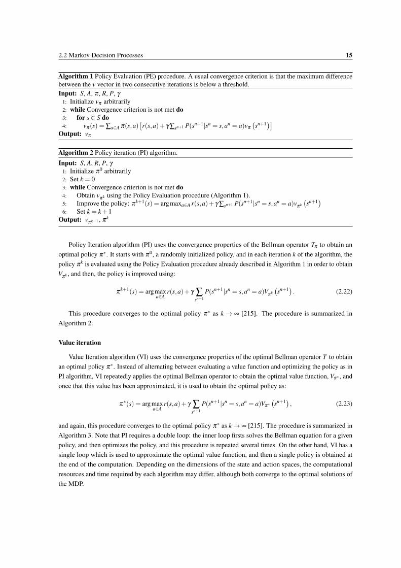
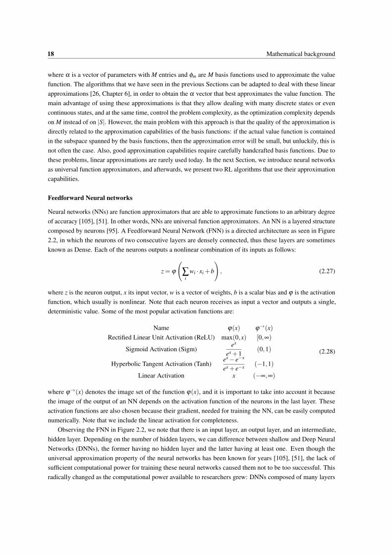
2.1 MDP basic interaction scheme. . . . . . . . . . . . . . . . . . . . . . . . . . . . . . . . . . . 92.2 Example of feedforward neural network. Each circle represents a neuron, which combines

non-linearly its inputs following (2.27). The inputs are x1 and x2, and the outputs are z1 and z2.There is a single hidden layer, which has three neurons. Note how each of the outputs z is anonlinear combination of the inputs x1 and x2. . . . . . . . . . . . . . . . . . . . . . . . . . . 19

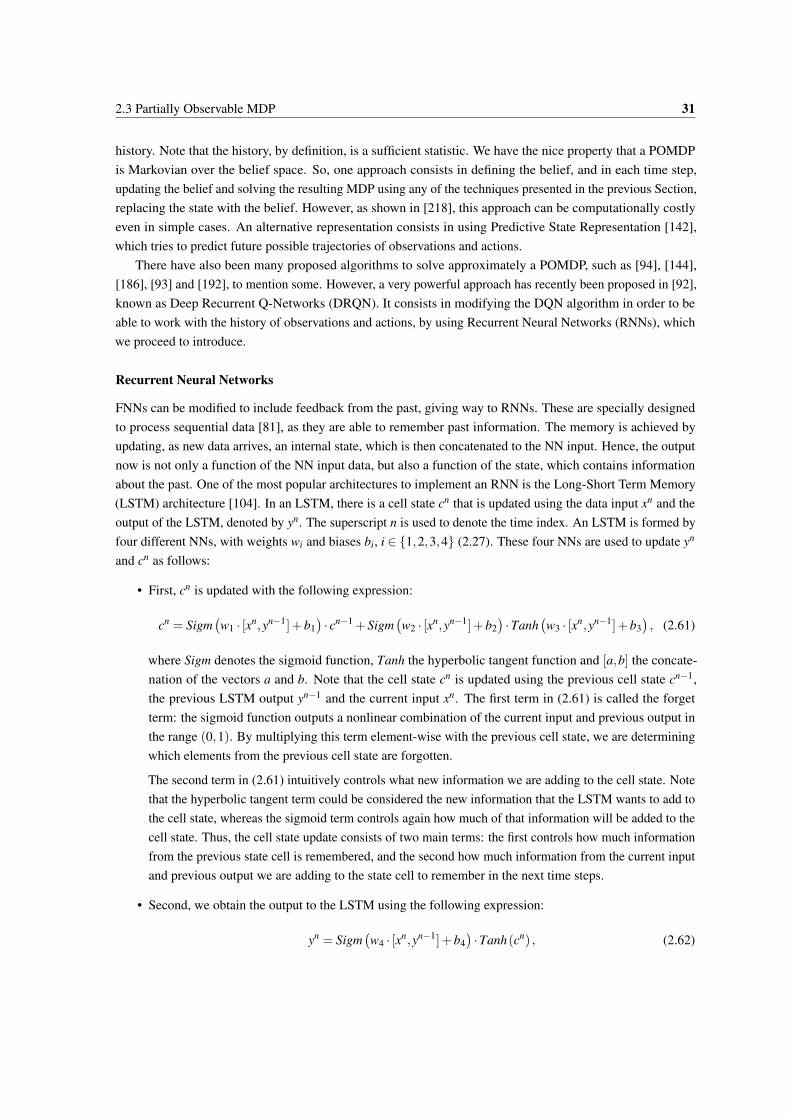
2.3 Illustration of the procedure of an LSTM for three time steps. The output yn is updated ineach time step using (2.62) and the cell state cn is updated using (2.61). The LSTM block iscomposed of four neural networks, which are the same for all time steps. Note that, in the firsttime step, it is necessary to provide an initial c0 and y0 in order to obtain c1 and y1. . . . . . . 32

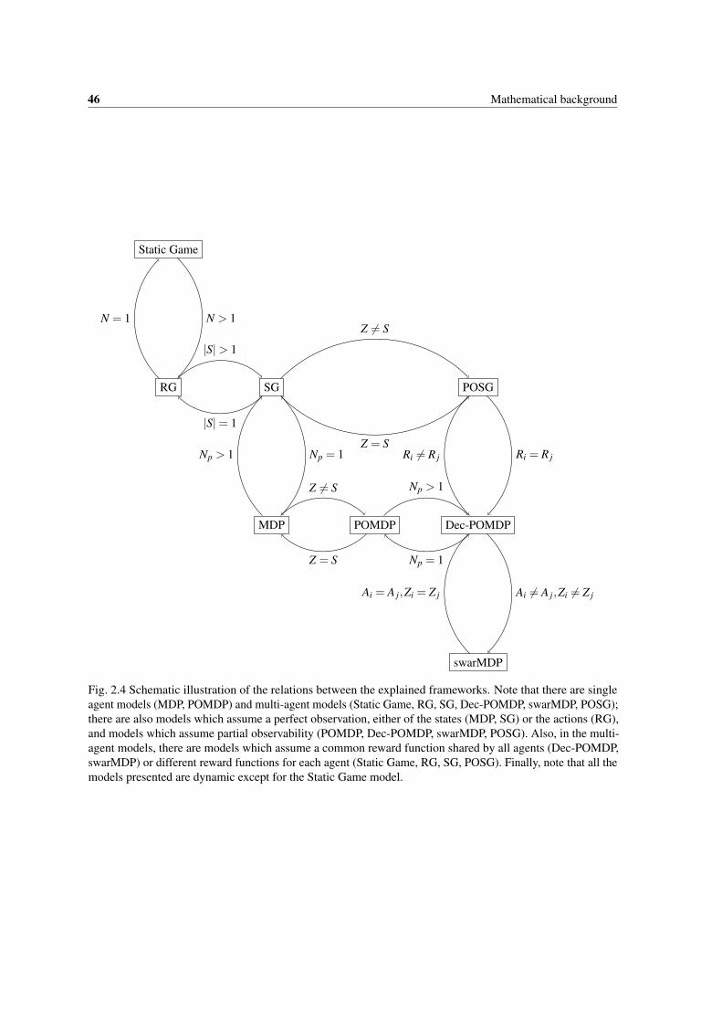
2.4 Schematic illustration of the relations between the explained frameworks. Note that there aresingle agent models (MDP, POMDP) and multi-agent models (Static Game, RG, SG, Dec-POMDP, swarMDP, POSG); there are also models which assume a perfect observation, eitherof the states (MDP, SG) or the actions (RG), and models which assume partial observability(POMDP, Dec-POMDP, swarMDP, POSG). Also, in the multi-agent models, there are modelswhich assume a common reward function shared by all agents (Dec-POMDP, swarMDP) ordifferent reward functions for each agent (Static Game, RG, SG, POSG). Finally, note that allthe models presented are dynamic except for the Static Game model. . . . . . . . . . . . . . . 46

3.1 Payoff matrices for the example games. Player 1 is the row player and player 2 is columnplayer. In each matrix, the payoff entries for each par of actions a = (a1,a2) are (r1(a),r2(a)). 48

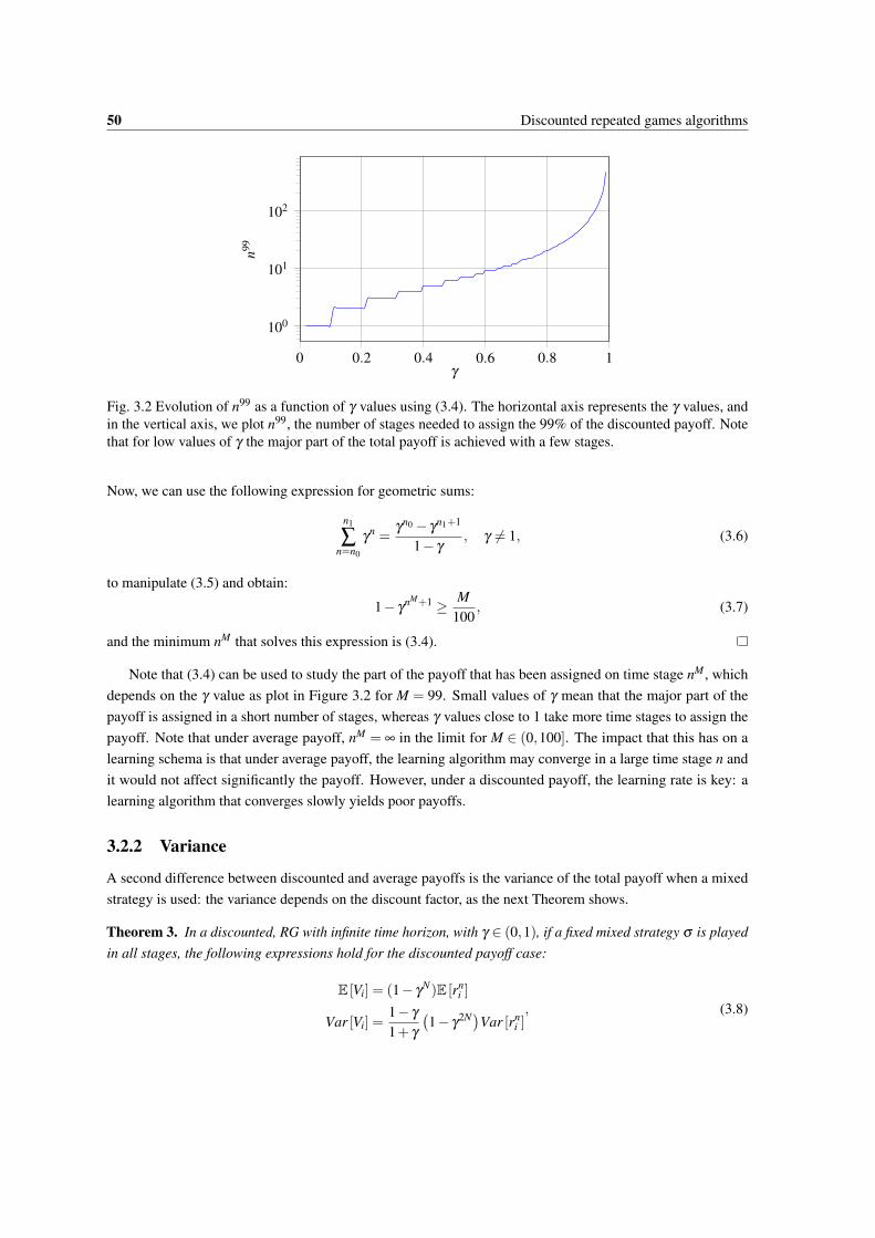
3.2 Evolution of n99 as a function of γ values using (3.4). The horizontal axis represents the γ

values, and in the vertical axis, we plot n99, the number of stages needed to assign the 99%of the discounted payoff. Note that for low values of γ the major part of the total payoff isachieved with a few stages. . . . . . . . . . . . . . . . . . . . . . . . . . . . . . . . . . . . . 50

3.3 Results of the standard deviation comparison simulation using MP. The horizontal axis repre-sents the γ values, and in the vertical axis, we plot the standard deviation of the payoff. Orangeline is for the theoretical average payoff case, using (3.9). Blue line is for the theoreticaldiscounted payoff case, using (3.8). Red lines are the empirical standard deviation obtainedunder simulation. Note how the standard deviation depends on γ under the discounted payoffcase. Also, note that the average payoff case gives in general lower deviations, except whenγ → 1. . . . . . . . . . . . . . . . . . . . . . . . . . . . . . . . . . . . . . . . . . . . . . . . 52

3.4 LEWIS block diagram. . . . . . . . . . . . . . . . . . . . . . . . . . . . . . . . . . . . . . . 53

xviii List of figures

3.5 Payoff results as a function of ε and γ in the PD game, using LEWIS. In the horizontal axis werepresent ε and in the vertical axis, the payoff of the players Vi. In this case, players learn tocooperate except when γ = 0 and both receive the same payoffs. Note how larger values of γ

and ε lead to larger payoffs. . . . . . . . . . . . . . . . . . . . . . . . . . . . . . . . . . . . . 583.6 Results of the simulation of LEWIS in self play, when both player 1 (P1) and player 2 (P2)

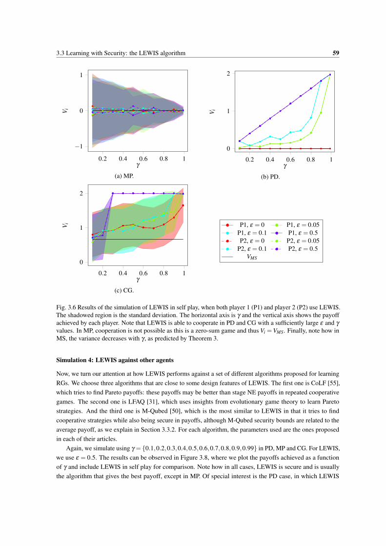
use LEWIS. The shadowed region is the standard deviation. The horizontal axis is γ and thevertical axis shows the payoff achieved by each player. Note that LEWIS is able to cooperate inPD and CG with a sufficiently large ε and γ values. In MP, cooperation is not possible as this isa zero-sum game and thus Vi =VMS. Finally, note how in MS, the variance decreases with γ , aspredicted by Theorem 3. . . . . . . . . . . . . . . . . . . . . . . . . . . . . . . . . . . . . . 59

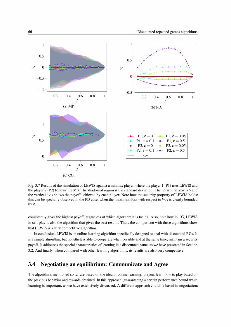
3.7 Results of the simulation of LEWIS against a minmax player, where the player 1 (P1) usesLEWIS and the player 2 (P2) follows the MS. The shadowed region is the standard deviation.The horizontal axis is γ and the vertical axis shows the payoff achieved by each player. Notehow the security property of LEWIS holds: this can be specially observed in the PD case, whenthe maximum loss with respect to VMS is clearly bounded by ε . . . . . . . . . . . . . . . . . . 60

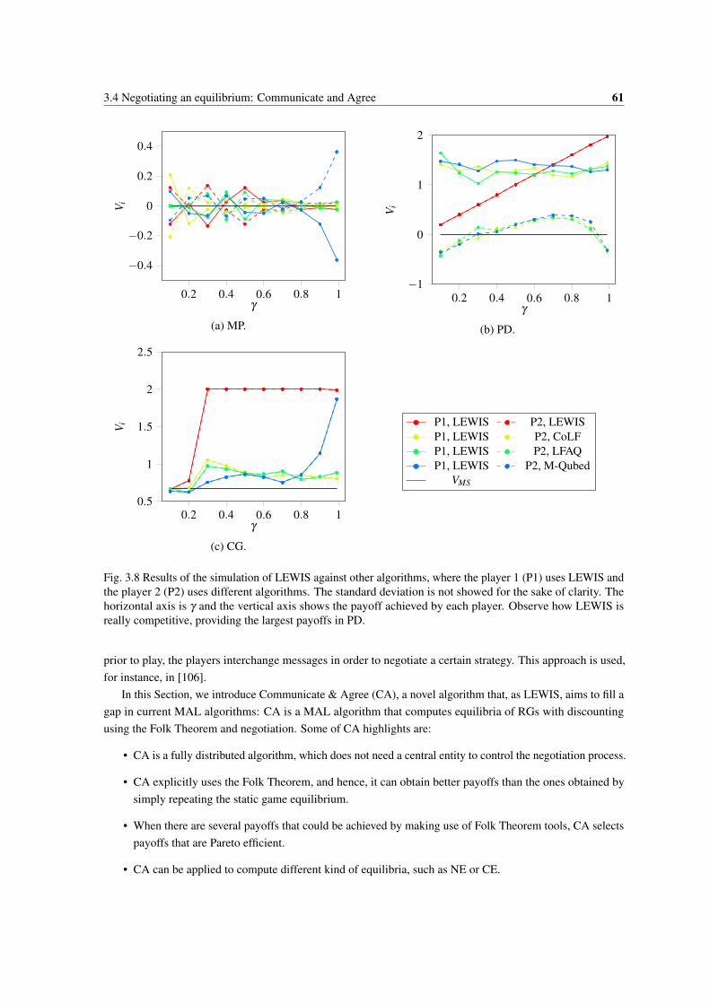
3.8 Results of the simulation of LEWIS against other algorithms, where the player 1 (P1) usesLEWIS and the player 2 (P2) uses different algorithms. The standard deviation is not showedfor the sake of clarity. The horizontal axis is γ and the vertical axis shows the payoff achievedby each player. Observe how LEWIS is really competitive, providing the largest payoffs in PD. 61

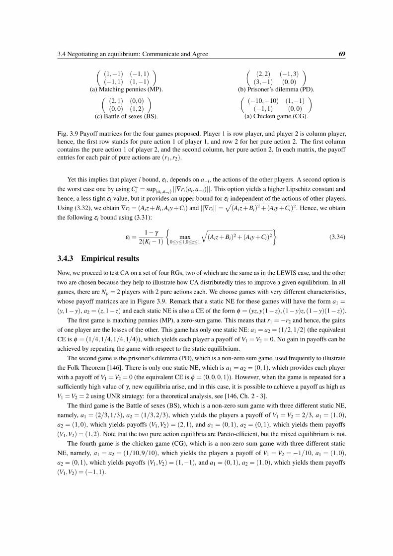
3.9 Payoff matrices for the four games proposed. Player 1 is row player, and player 2 is columnplayer, hence, the first row stands for pure action 1 of player 1, and row 2 for her pure action 2.The first column contains the pure action 1 of player 2, and the second column, her pure action2. In each matrix, the payoff entries for each pair of pure actions are (r1,r2). . . . . . . . . . . 69

3.10 Average values of ξ for each sampling method. Equispaced sampling is ’eq’, random uniformsampling is ’unif’ and ’RM’ stands for regret-matching results. We observe that, as we increasethe number of communications allowed Nc, the error ξ decreases. Recall that ξ measures howfar the CA results are from the theoretical Pareto frontier (see (3.36)). Thus, lower is better, asit implies that the players achieve a payoff closer to the Pareto frontier. Note that a greater Nc

allows getting closer to the Pareto frontier. The sampling methods order, from the worst to thebest performance, are equispaced, random uniform and SOO. Even though in SOO we use astricter limitation, as we limit in samples instead of communications, it outperforms the othersampling methods. . . . . . . . . . . . . . . . . . . . . . . . . . . . . . . . . . . . . . . . . 71

3.11 Payoff results: for each game, we represent the average payoff increment ∆Vi between CA andRM for different values of γ . Thus, higher is better, as it means that CA provides better payoffsthan RM. We use four sampling methods for CA: equispaced (eq), random uniform (rn), SOOwith λ = 0.5 (op1) and SOO with λ = 1 (op2), for NE and CE. When CA takes advantage ofthe Folk Theorem, it outperforms RM, as happens in PD. And when using the Folk Theoremprovides no advantage in payoffs, as in MP, BS and CG, CA is not worse than RM, as expected. 72

List of figures xix

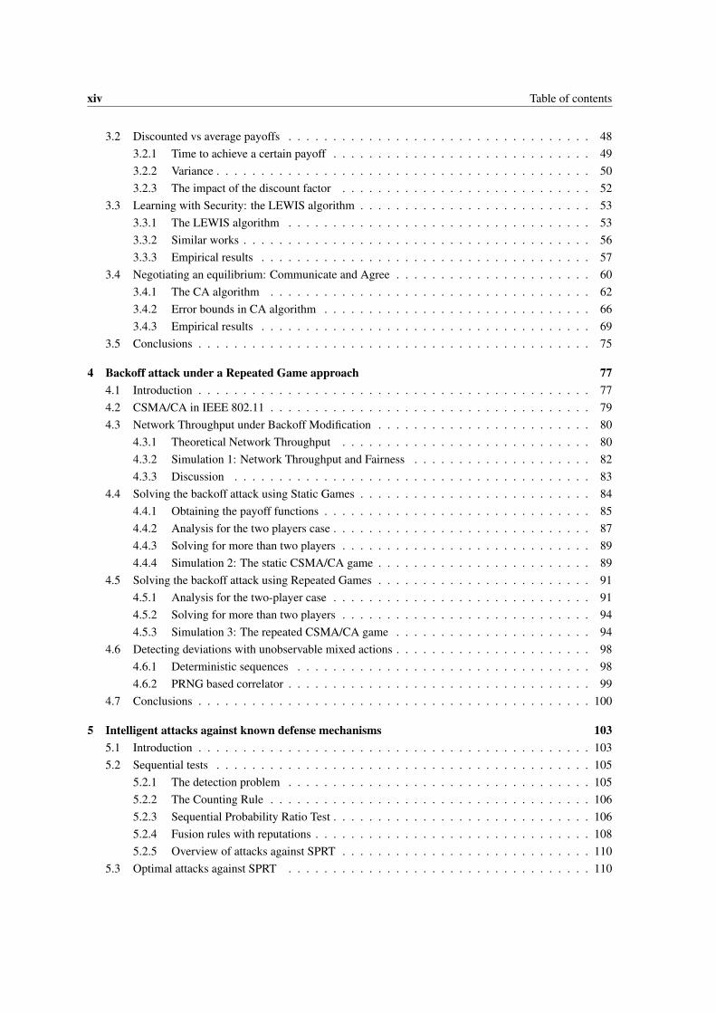
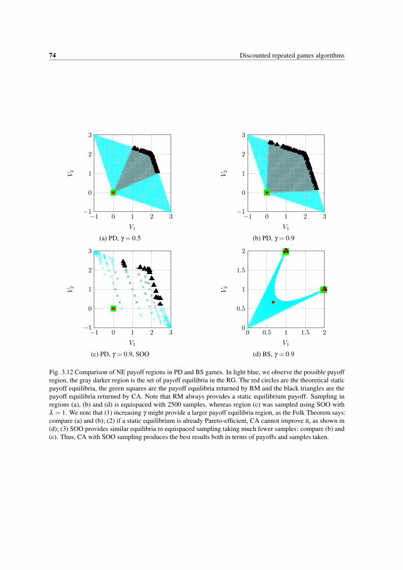
3.12 Comparison of NE payoff regions in PD and BS games. In light blue, we observe the possiblepayoff region, the gray darker region is the set of payoff equilibria in the RG. The red circlesare the theoretical static payoff equilibria, the green squares are the payoff equilibria returnedby RM and the black triangles are the payoff equilibria returned by CA. Note that RM alwaysprovides a static equilibrium payoff. Sampling in regions (a), (b) and (d) is equispaced with2500 samples, whereas region (c) was sampled using SOO with λ = 1. We note that (1)increasing γ might provide a larger payoff equilibria region, as the Folk Theorem says: compare(a) and (b); (2) if a static equilibrium is already Pareto-efficient, CA cannot improve it, asshown in (d); (3) SOO provides similar equilibria to equispaced sampling taking much fewersamples: compare (b) and (c). Thus, CA with SOO sampling produces the best results both interms of payoffs and samples taken. . . . . . . . . . . . . . . . . . . . . . . . . . . . . . . . 74

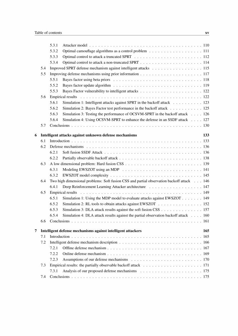
4.1 Network scheme for the case that there are n1 GSs and n2 ASs. GSs respect 802.11 binaryexponential backoff, whereas ASs can choose to use it or to use a uniform backoff. . . . . . . 79

4.2 Throughput S results for the simulation, using Bianchi’s model with short payload, Tp,l , (a-d),and long payload, Tp,l , (e-h). In cases (a) and (e), there are no ASs; in cases (b-d) and (f-h)there are ASs. S1 is the throughput of normal stations, S2 the throughput of malicious stations.Note how having ASs significantly decreases the throughput of GSs. . . . . . . . . . . . . . . 83

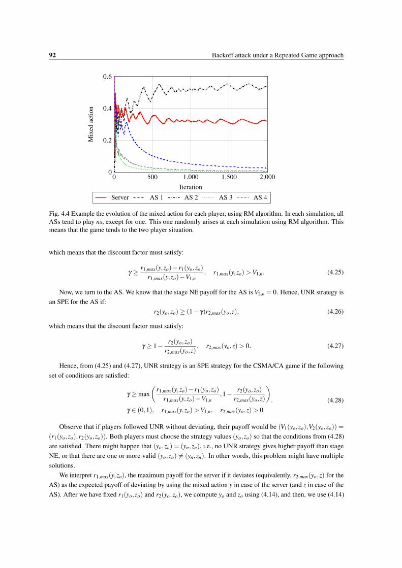
4.3 Histogram of actions obtained using RM algorithm, for I = 5 sensors and variable number ofASs. Each histogram is computed using 5 bins. Observe that the action of the server does notvary significantly, whereas the actions of the ASs do. Also, observe how as n2 increases, theASs histogram presents two peaks: the biggest close to 0 and a smaller peak at another mixedaction value. This hints that the game tends to the two player case when there are many ASs:all but one AS tend to behave as GSs. . . . . . . . . . . . . . . . . . . . . . . . . . . . . . . 91

4.4 Example the evolution of the mixed action for each player, using RM algorithm. In eachsimulation, all ASs tend to play ns, except for one. This one randomly arises at each simulationusing RM algorithm. This means that the game tends to the two player situation. . . . . . . . . 92

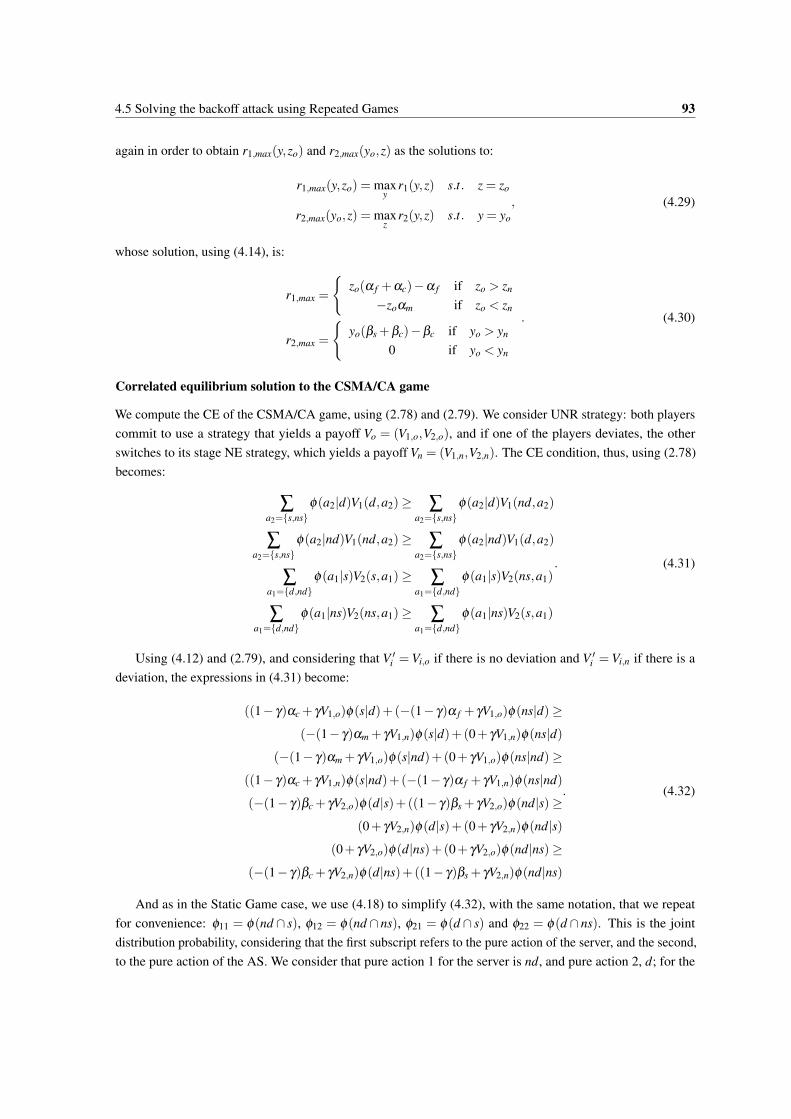
4.5 Payoff V obtained for the server and ASs, using CA. The error bars show the maximum andminimum values achieved. For ASs, we plot the mean values, computed among the n2 ASs inthe setup. We can observe that CA never performs worse than RM, and when there is a lownumber of ASs it provides a significant payoff gain to both server and ASs. . . . . . . . . . . 95

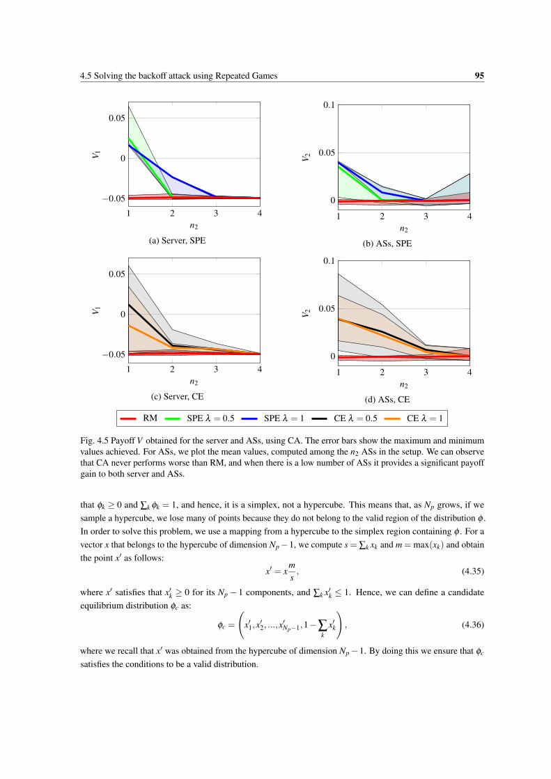
4.6 Payoff region when n2 = 1, using SPE and CE. The light region are all possible payoffs, the redsquare is the static NE that RM provides, the blue circles are the points that CA samples andthe circles with a black cross are those that are valid equilibria for the RG, i.e., there is a greaterpayoff for both players than their stage NE payoff. Observe that the SPE region is contained inthe CE region. . . . . . . . . . . . . . . . . . . . . . . . . . . . . . . . . . . . . . . . . . . . 96

xx List of figures

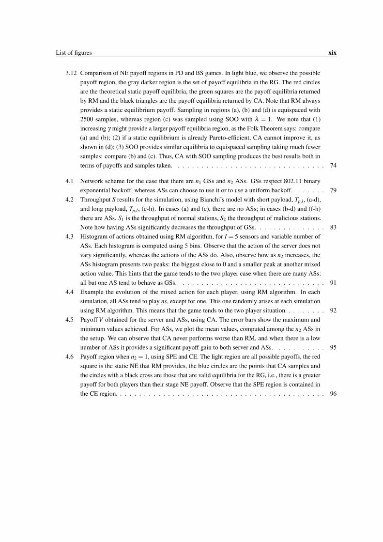
4.7 Payoff V obtained for the server and the ASs, using LEWIS for ε = {0,0.1}, compared to thesecurity payoff and the RM payoff. The shadow regions represent the maximum and minimumvalues obtained: note that in some cases LEWIS acts deterministically. The security conditionof LEWIS is satisfied in all cases: note that this condition depends on the minmax strategypayoff (MS) and the ε value. In case of the ASs, the security payoff, the RM payoff and theLEWIS payoff when ε = 0 are nearly the same: note that the ASs have some loss when ε = 0.1,although the security condition holds, as the loss is lower than ε . In case of the the Server, thesecurity payoff and the RM payoff are very close again, but the server is able to improve itspayoff by using LEWIS for all ε values tested. . . . . . . . . . . . . . . . . . . . . . . . . . . 97

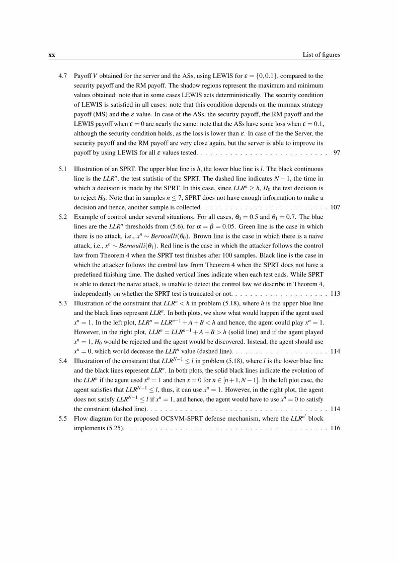
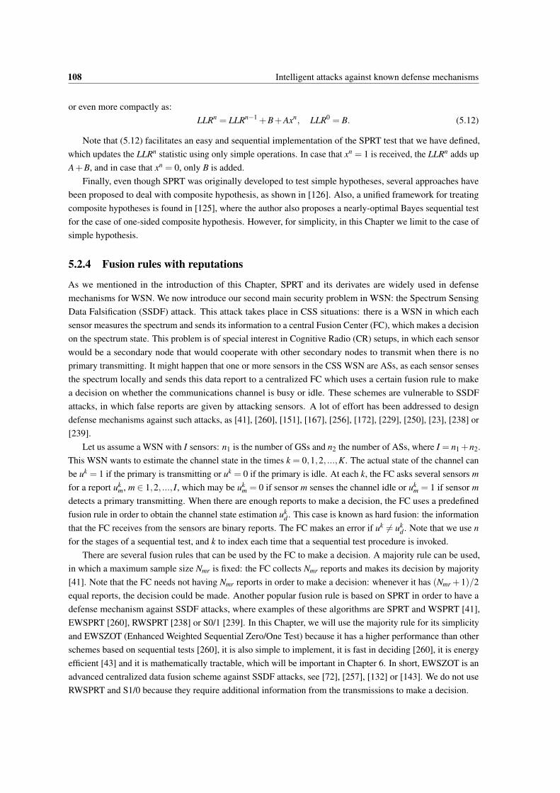
5.1 Illustration of an SPRT. The upper blue line is h, the lower blue line is l. The black continuousline is the LLRn, the test statistic of the SPRT. The dashed line indicates N− 1, the time inwhich a decision is made by the SPRT. In this case, since LLRn ≥ h, H0 the test decision isto reject H0. Note that in samples n≤ 7, SPRT does not have enough information to make adecision and hence, another sample is collected. . . . . . . . . . . . . . . . . . . . . . . . . . 107

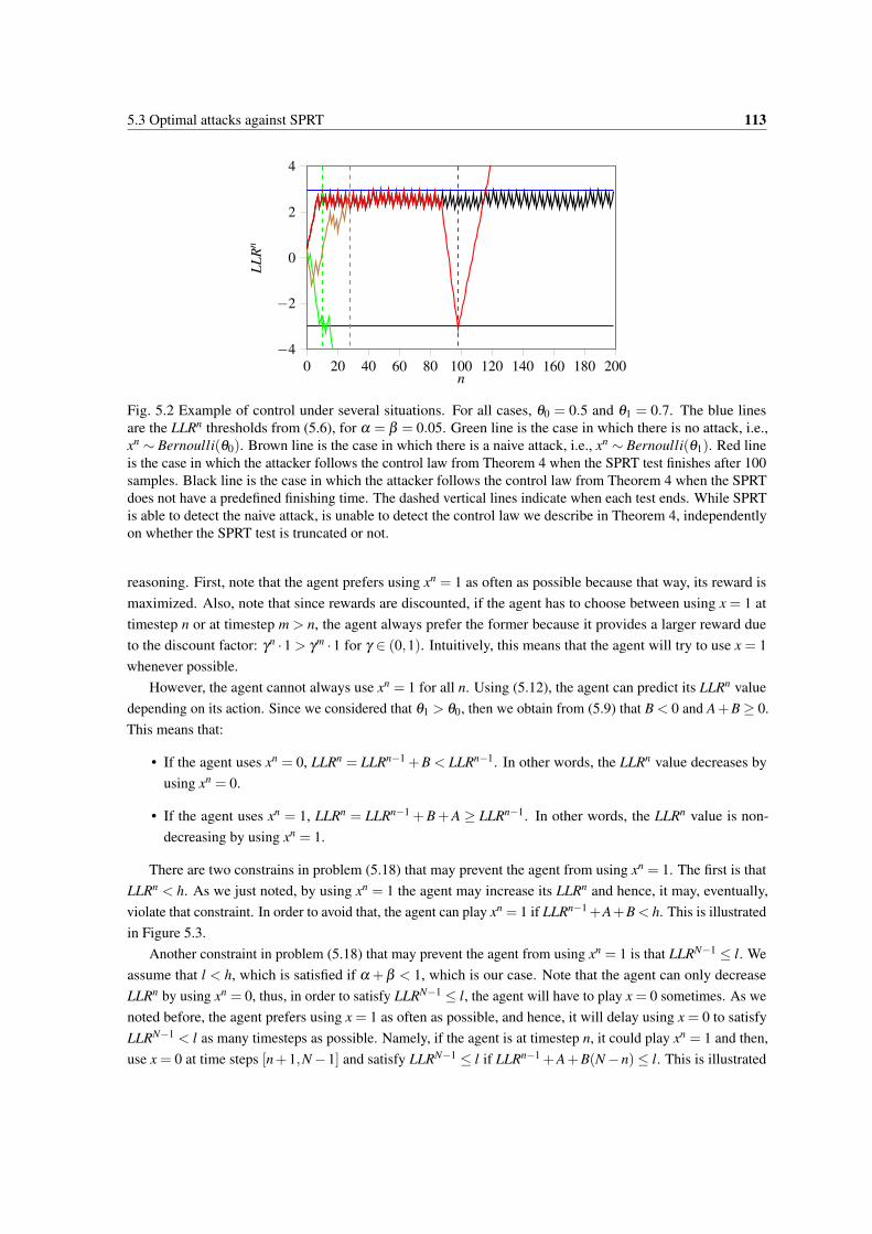
5.2 Example of control under several situations. For all cases, θ0 = 0.5 and θ1 = 0.7. The bluelines are the LLRn thresholds from (5.6), for α = β = 0.05. Green line is the case in whichthere is no attack, i.e., xn ∼ Bernoulli(θ0). Brown line is the case in which there is a naiveattack, i.e., xn ∼ Bernoulli(θ1). Red line is the case in which the attacker follows the controllaw from Theorem 4 when the SPRT test finishes after 100 samples. Black line is the case inwhich the attacker follows the control law from Theorem 4 when the SPRT does not have apredefined finishing time. The dashed vertical lines indicate when each test ends. While SPRTis able to detect the naive attack, is unable to detect the control law we describe in Theorem 4,independently on whether the SPRT test is truncated or not. . . . . . . . . . . . . . . . . . . . 113

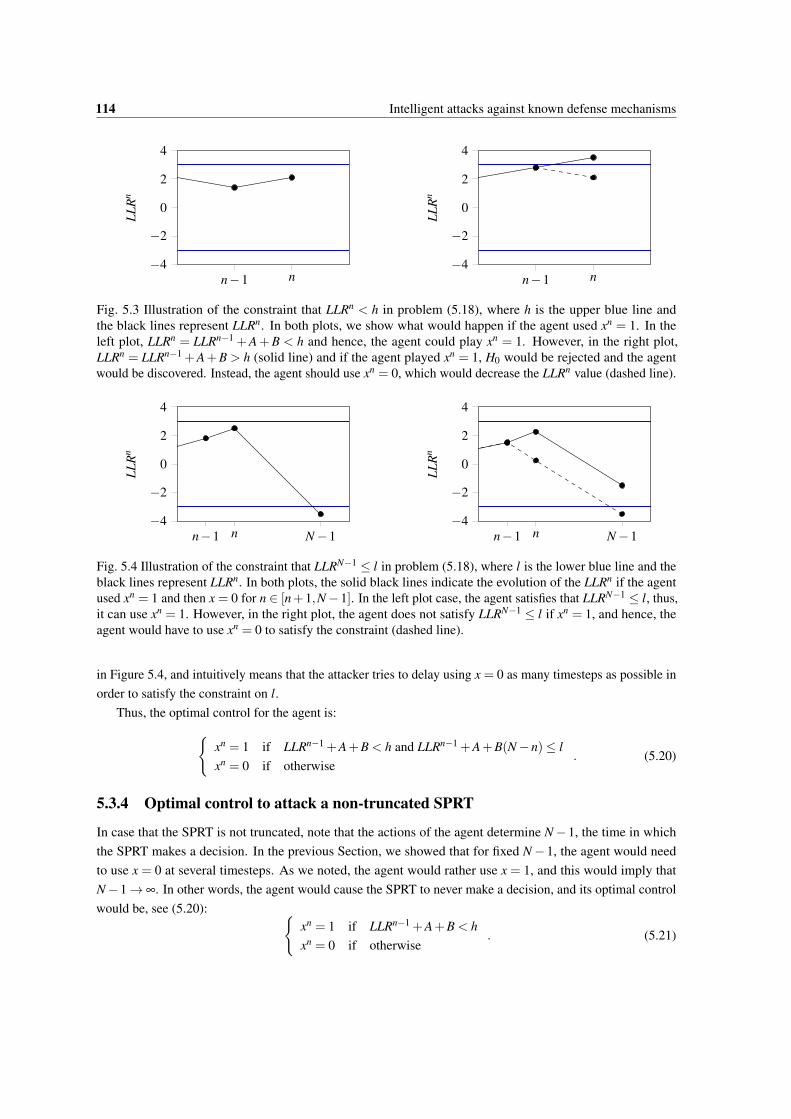
5.3 Illustration of the constraint that LLRn < h in problem (5.18), where h is the upper blue lineand the black lines represent LLRn. In both plots, we show what would happen if the agent usedxn = 1. In the left plot, LLRn = LLRn−1 +A+B < h and hence, the agent could play xn = 1.However, in the right plot, LLRn = LLRn−1 +A+B > h (solid line) and if the agent playedxn = 1, H0 would be rejected and the agent would be discovered. Instead, the agent should usexn = 0, which would decrease the LLRn value (dashed line). . . . . . . . . . . . . . . . . . . . 114

5.4 Illustration of the constraint that LLRN−1 ≤ l in problem (5.18), where l is the lower blue lineand the black lines represent LLRn. In both plots, the solid black lines indicate the evolution ofthe LLRn if the agent used xn = 1 and then x = 0 for n ∈ [n+1,N−1]. In the left plot case, theagent satisfies that LLRN−1 ≤ l, thus, it can use xn = 1. However, in the right plot, the agentdoes not satisfy LLRN−1 ≤ l if xn = 1, and hence, the agent would have to use xn = 0 to satisfythe constraint (dashed line). . . . . . . . . . . . . . . . . . . . . . . . . . . . . . . . . . . . . 114

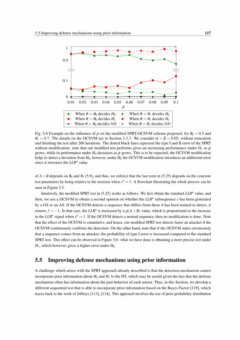
5.5 Flow diagram for the proposed OCSVM-SPRT defense mechanism, where the LLRn′ blockimplements (5.25). . . . . . . . . . . . . . . . . . . . . . . . . . . . . . . . . . . . . . . . . 116

List of figures xxi

5.6 Example on the influence of ρ on the modified SPRT-OCSVM scheme proposed, for θ0 = 0.5and θ1 = 0.7. The details on the OCSVM are in Section 3.3.3. We consider α = β = 0.05,without truncation and finishing the test after 200 iterations. The dotted black lines represent thetype I and II error of the SPRT without modification: note that our modified test performs givesan increasing performance under H1 as ρ grows, while its performance under H0 decreases asρ grows. This is to be expected: the OCSVM modification helps to detect a deviation from H0,however, under H0 the OCSVM modification introduces an additional error since it increasesthe LLRn value. . . . . . . . . . . . . . . . . . . . . . . . . . . . . . . . . . . . . . . . . . . 117

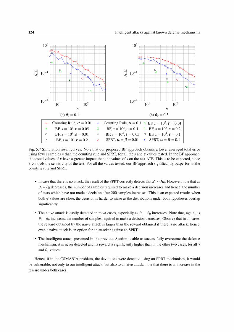
5.7 Simulation result curves. Note that our proposed BF approach obtains a lower averaged totalerror using fewer samples n than the counting rule and SPRT, for all the s and ε values tested.In the BF approach, the tested values of ε have a greater impact than the values of s on the testATE. This is to be expected, since ε controls the sensitivity of the test. For all the values tested,our BF approach significantly outperforms the counting rule and SPRT. . . . . . . . . . . . . 124

5.8 Proportion of H0 rejections for the different schemes proposed as a function of θ0. The dottedlines correspond to the α and 1− β values of the tests. Note that under H0, i.e., NA, ourproposed SPRT-OCSVM performs worse than SPRT, rejecting H0 more often; and under H1,SPRT-OCSVM works better than SPRT, as we advanced in Figure 5.6. However, note that theimprovement in detecting an AS following the control law from Theorem 4 is dramatic: whileSPRT is never able to detect it, SPRT-OCSVM always detects the AS. . . . . . . . . . . . . . 127

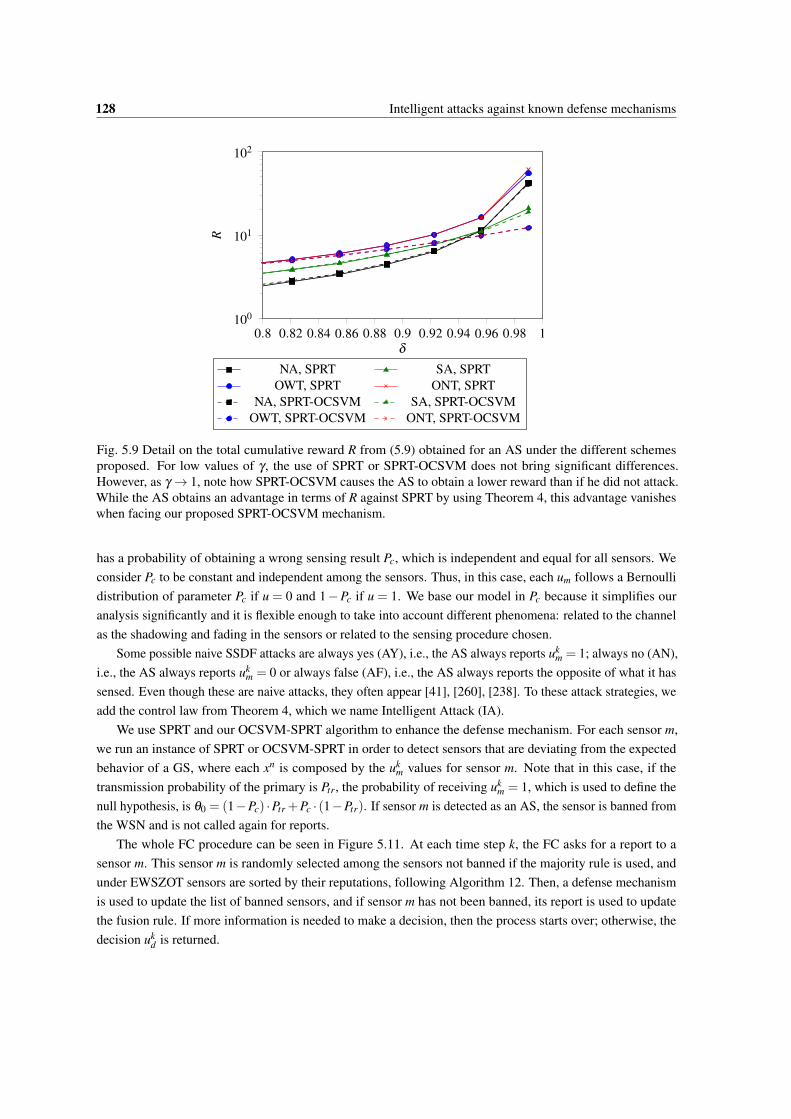
5.9 Detail on the total cumulative reward R from (5.9) obtained for an AS under the differentschemes proposed. For low values of γ , the use of SPRT or SPRT-OCSVM does not bringsignificant differences. However, as γ → 1, note how SPRT-OCSVM causes the AS to obtain alower reward than if he did not attack. While the AS obtains an advantage in terms of R againstSPRT by using Theorem 4, this advantage vanishes when facing our proposed SPRT-OCSVMmechanism. . . . . . . . . . . . . . . . . . . . . . . . . . . . . . . . . . . . . . . . . . . . . 128

5.10 Example of detection for θ0 = 0.5 and θ1 = 0.7. The blue lines are the LLRn thresholds from(5.6). In both cases, we compare a realization of the control law from Theorem 4 withouttruncation, using SPRT (black) and SPRT-OCSVM (red). The dashed vertical line indicate wheneach test ends. Observe that, as in Figure 5.2, the SPRT is unable to detect the attack. However,SPRT-OCSVM is able to do so: when it believes that there is an AS, it starts increasing slowlythe LLRn value using (5.25). Note that this means that eventually, the AS is detected. . . . . . 129

5.11 Flow diagram for each time step k of the SSDF problem. The sensor list contains the list ofsensors banned and not banned, and hence, it is used to determine to which sensors the FC asksfor a report and takes into account in the fusion procedure. . . . . . . . . . . . . . . . . . . . 129

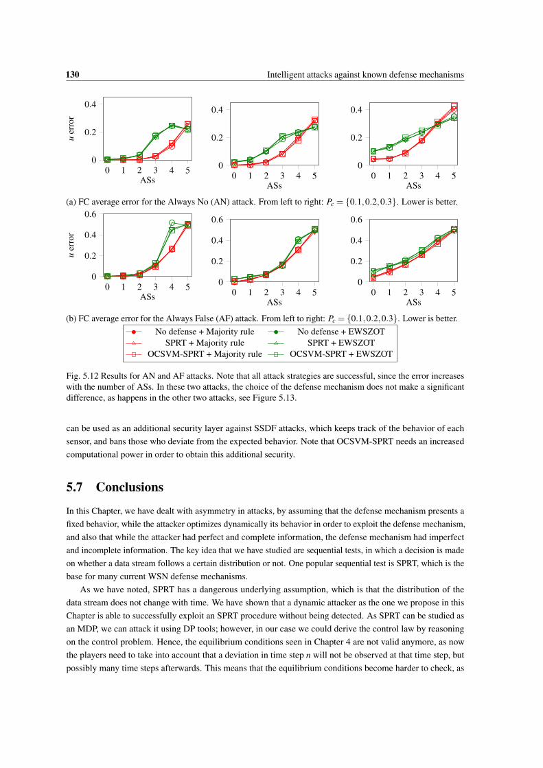
5.12 Results for AN and AF attacks. Note that all attack strategies are successful, since the errorincreases with the number of ASs. In these two attacks, the choice of the defense mechanismdoes not make a significant difference, as happens in the other two attacks, see Figure 5.13. . . 130

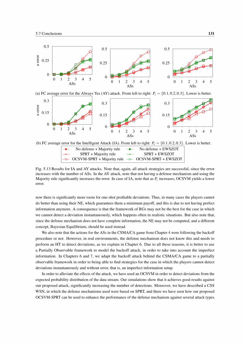
5.13 Results for IA and AY attacks. Note that, again, all attack strategies are successful, sincethe error increases with the number of ASs. In the AY attack, note that not having a defensemechanism and using the Majority rule significantly increases the error. In case of IA, note thatas Pc increases, OCSVM yields a lower error. . . . . . . . . . . . . . . . . . . . . . . . . . . 131

xxii List of figures

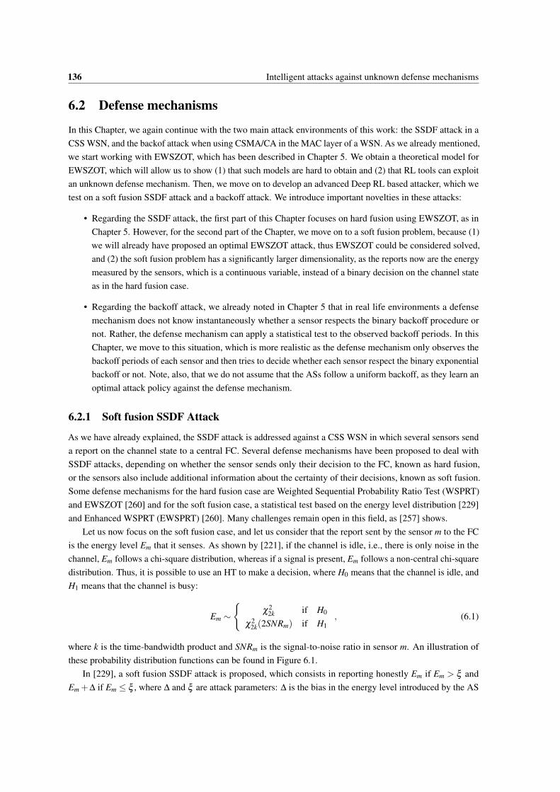
6.1 Illustration of the probability distribution function (pdfs) of the chi-squared distributions from(6.1). The thick pdf corresponds to the H0 case: the chi-squared χ2

2k distribution; and the thinnerpdfs correspond to the H1 case: the non-central chi-squared χ2

2k(2SNRm) distributions for SNRvalues {2,4,6,8,10}, from left to right in the plot. For all curves, k = 5 is the time-bandwidthparameter. Observe that, as the SNR increases, the pdf curves are more separated for H0 and H1.137

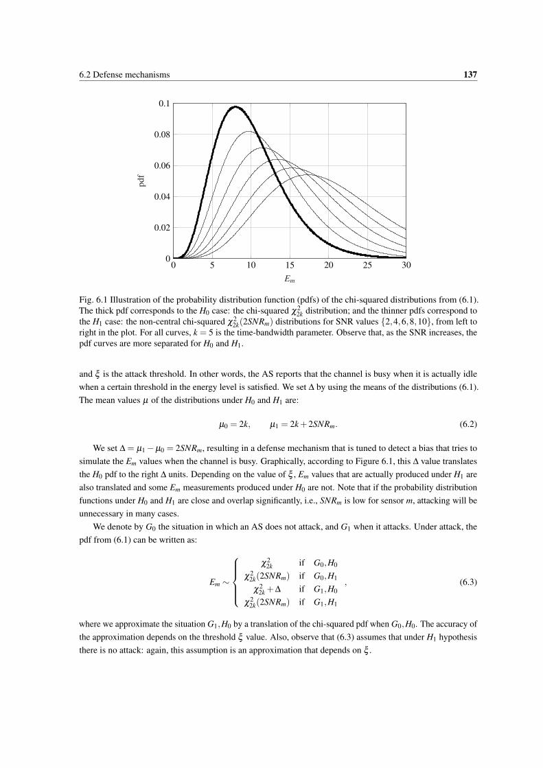
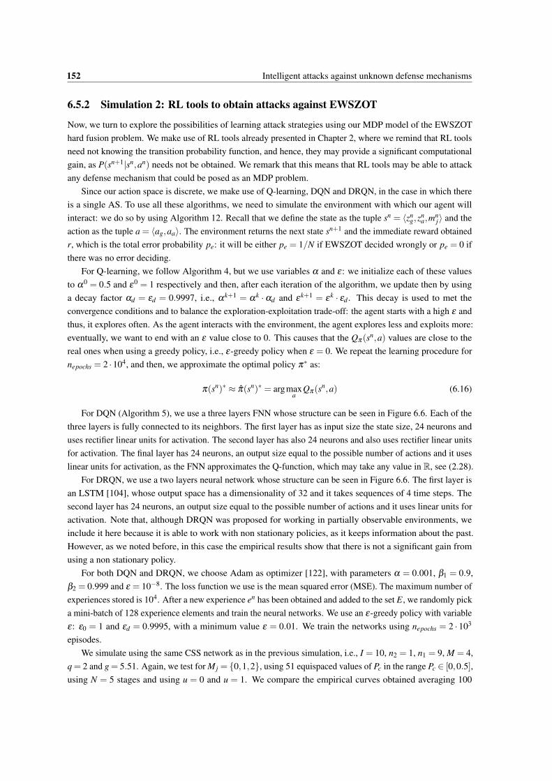
6.2 EWSZOT algorithm modeling illustration. Each HT receives as input a reputation vector and anumber of jammed sensors and produces a certain number k of updated reputation vectors andjammed sensors. These vectors are used as inputs to new tests in next stages. Each HT has asmany k outputs as leaves. Each HT procedure is found using Algorithm 15. . . . . . . . . . . 142

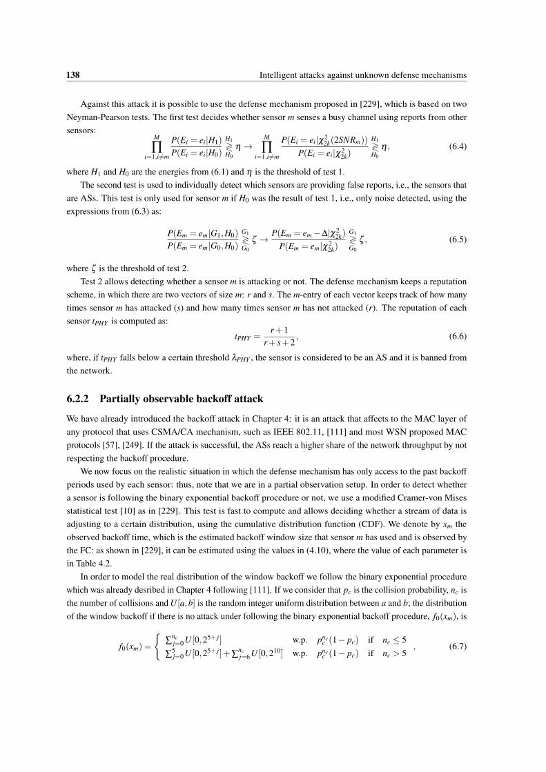
6.3 Illustration of EWSZOT HT tree. Each node contains the sequence of reports. For simplicity,we plot part of the tree when M = 3. Leaves are the thicker nodes. Observe that the leaves mayhappen when any of the final conditions from (5.14) is satisfied. . . . . . . . . . . . . . . . . 142

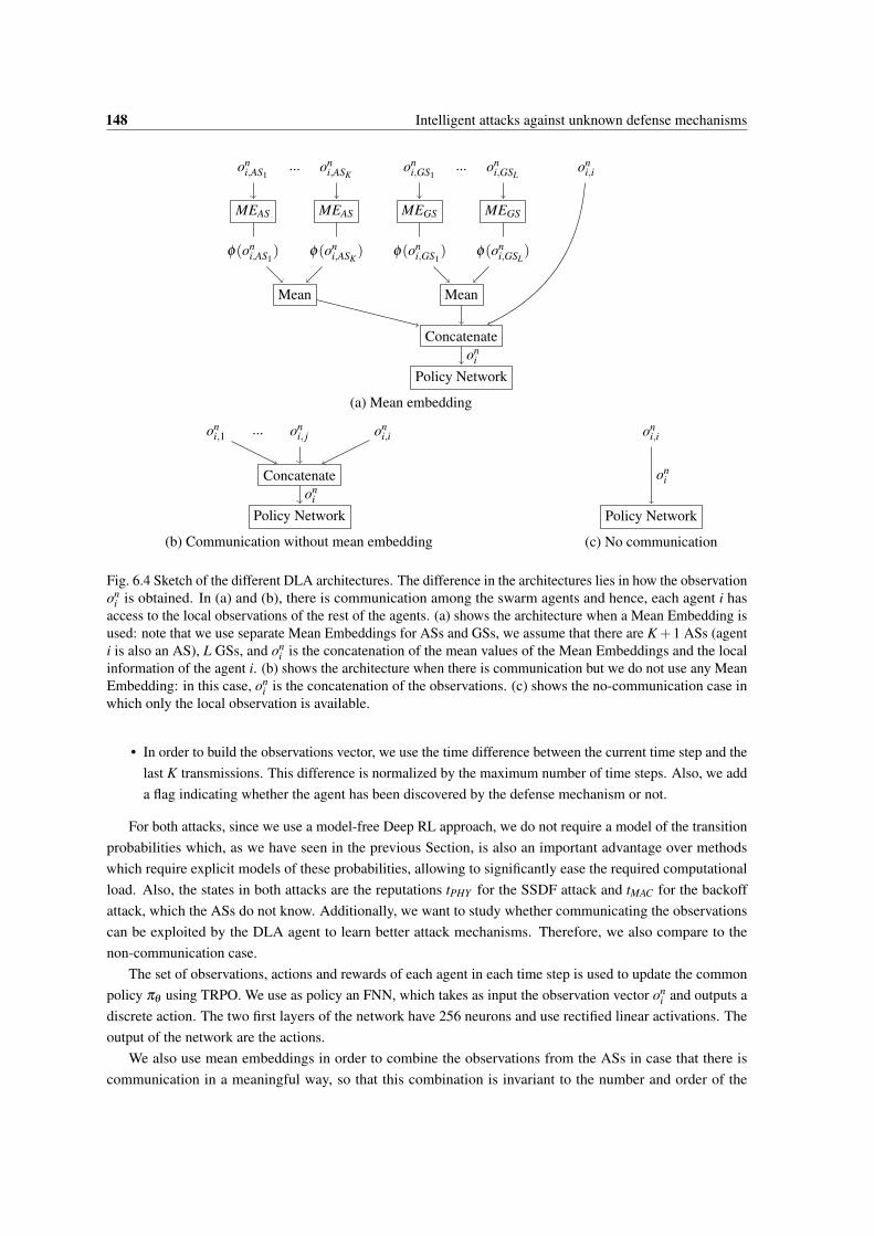
6.4 Sketch of the different DLA architectures. The difference in the architectures lies in how theobservation on

i is obtained. In (a) and (b), there is communication among the swarm agents andhence, each agent i has access to the local observations of the rest of the agents. (a) shows thearchitecture when a Mean Embedding is used: note that we use separate Mean Embeddingsfor ASs and GSs, we assume that there are K +1 ASs (agent i is also an AS), L GSs, and on

i

is the concatenation of the mean values of the Mean Embeddings and the local informationof the agent i. (b) shows the architecture when there is communication but we do not useany Mean Embedding: in this case, on

i is the concatenation of the observations. (c) shows theno-communication case in which only the local observation is available. . . . . . . . . . . . . 148

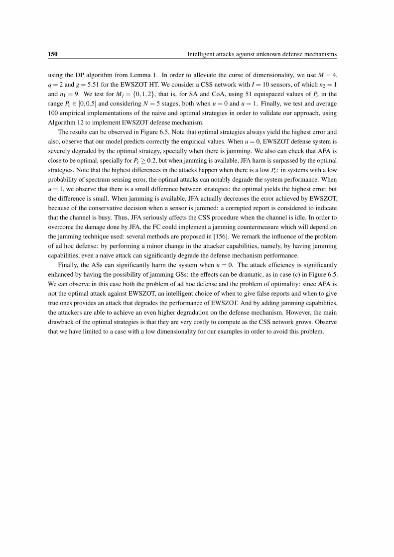
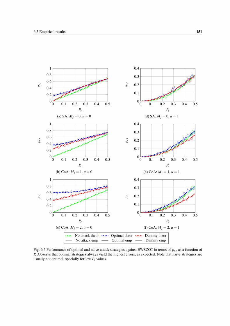
6.5 Performance of optimal and naive attack strategies against EWSZOT in terms of pe,t as afunction of Pc.Observe that optimal strategies always yield the highest errors, as expected. Notethat naive strategies are usually not optimal, specially for low Pc values. . . . . . . . . . . . . 151

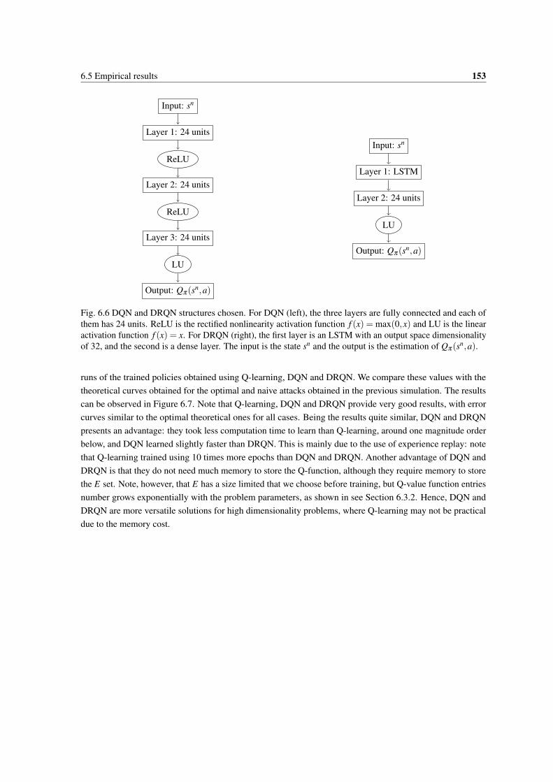
6.6 DQN and DRQN structures chosen. For DQN (left), the three layers are fully connectedand each of them has 24 units. ReLU is the rectified nonlinearity activation function f (x) =max(0,x) and LU is the linear activation function f (x) = x. For DRQN (right), the first layer isan LSTM with an output space dimensionality of 32, and the second is a dense layer. The inputis the state sn and the output is the estimation of Qπ(sn,a). . . . . . . . . . . . . . . . . . . . 153

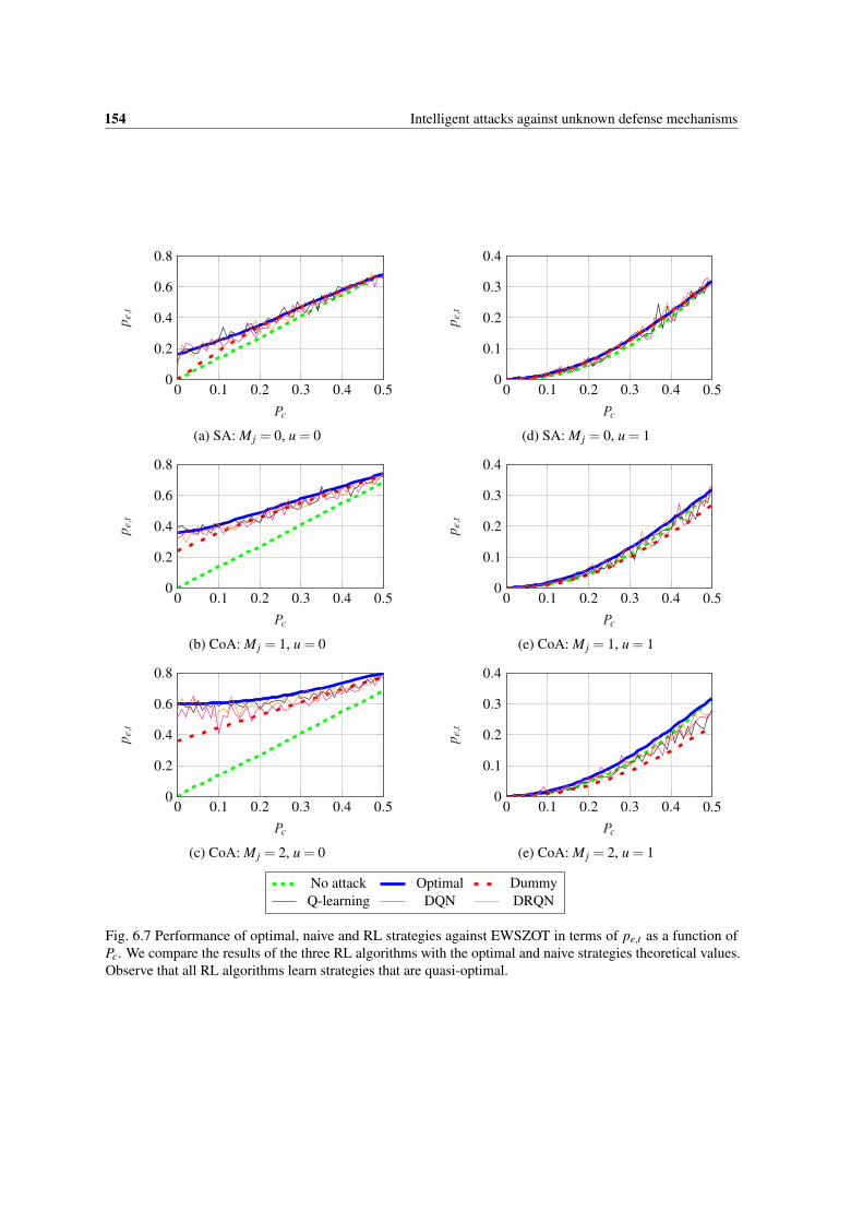
6.7 Performance of optimal, naive and RL strategies against EWSZOT in terms of pe,t as a functionof Pc. We compare the results of the three RL algorithms with the optimal and naive strategiestheoretical values. Observe that all RL algorithms learn strategies that are quasi-optimal. . . . 154

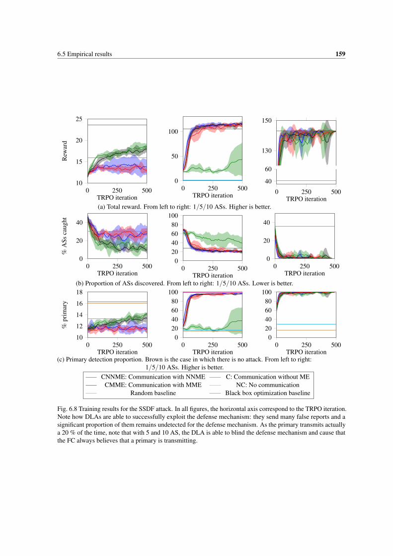
6.8 Training results for the SSDF attack. In all figures, the horizontal axis correspond to the TRPOiteration. Note how DLAs are able to successfully exploit the defense mechanism: they sendmany false reports and a significant proportion of them remains undetected for the defensemechanism. As the primary transmits actually a 20 % of the time, note that with 5 and 10 AS,the DLA is able to blind the defense mechanism and cause that the FC always believes that aprimary is transmitting. . . . . . . . . . . . . . . . . . . . . . . . . . . . . . . . . . . . . . . 159

List of figures xxiii

6.9 Examples of learned SSDF attack policies for the DLA, using CNNME and without communi-cation (NC) with 5 ASs. For comparison purposes we set λPHY = 0.5. We plot the normalizedenergy that each sensor reports, where blue are the energies reported by GSs, red are theenergies reported by discovered ASs and green are the energies reported by undiscovered ASs.In the CNNME case, the agents learn to transmit high levels of energy and not being discovered(a), whereas in NC case, there are times in which sensors are discovered due to their lack ofcooperation (c). In general, in NC, ASs report energies lower than in the CNME case (compare(a) to (b)): cooperation helps obtaining a more aggressive policy which, at the same time, allowsthe ASs to camouflage. . . . . . . . . . . . . . . . . . . . . . . . . . . . . . . . . . . . . . . 161

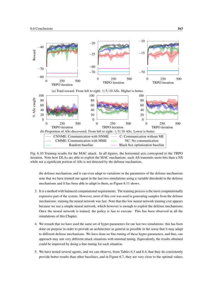
6.10 Training results for the MAC attack. In all figures, the horizontal axis correspond to the TRPOiteration. Note how DLAs are able to exploit the MAC mechanism: each AS transmits morebits than a NS while not a significant portion of ASs is not detected by the defense mechanism. 163

6.11 Examples of learned backoff attack policies for the DLA, using CNNME with 10 ASs. Thecolored lines are the tMAC values, and each dot indicates that the defense mechanism has beeninvoked. Blue is for GSs, green for ASs not discovered and red for discovered ASs. The blackline is λMAC. Note how the ASs are able to adapt to the different values of λMAC. . . . . . . . . 164

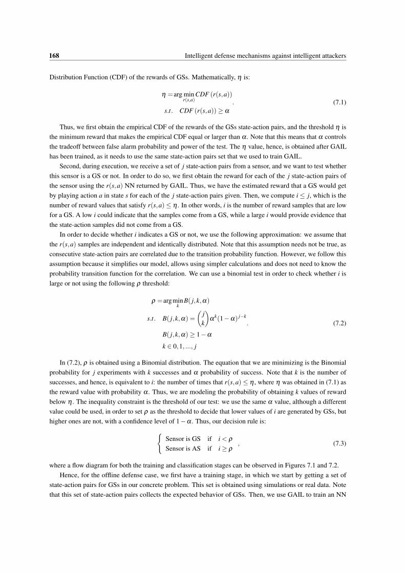
7.1 Flow diagram for the training stage of the proposed defense mechanism, both for online andoffline cases. . . . . . . . . . . . . . . . . . . . . . . . . . . . . . . . . . . . . . . . . . . . . 169

7.2 Flow diagram for the classification stage of our proposed defense mechanism, for both onlineand offline cases. . . . . . . . . . . . . . . . . . . . . . . . . . . . . . . . . . . . . . . . . . 169

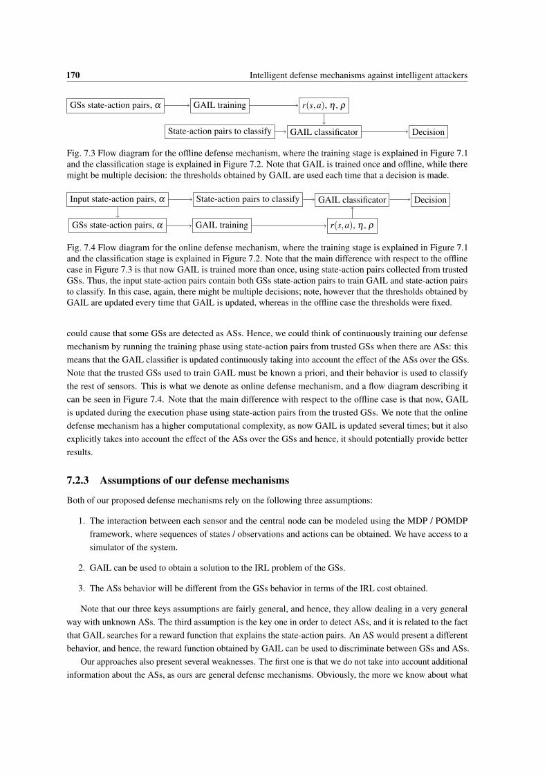
7.3 Flow diagram for the offline defense mechanism, where the training stage is explained in Figure7.1 and the classification stage is explained in Figure 7.2. Note that GAIL is trained once andoffline, while there might be multiple decision: the thresholds obtained by GAIL are used eachtime that a decision is made. . . . . . . . . . . . . . . . . . . . . . . . . . . . . . . . . . . . 170

7.4 Flow diagram for the online defense mechanism, where the training stage is explained in Figure7.1 and the classification stage is explained in Figure 7.2. Note that the main difference withrespect to the offline case in Figure 7.3 is that now GAIL is trained more than once, usingstate-action pairs collected from trusted GSs. Thus, the input state-action pairs contain bothGSs state-action pairs to train GAIL and state-action pairs to classify. In this case, again, theremight be multiple decisions; note, however that the thresholds obtained by GAIL are updatedevery time that GAIL is updated, whereas in the offline case the thresholds were fixed. . . . . 170

7.5 Results evolution during training for the proposed backoff attack setup. In all figures, thehorizontal axis correspond to the TRPO iteration. Note how both defense mechanisms improvein all measures the baseline, except for the increase in false alarm, i.e., the probability ofbanning GSs. . . . . . . . . . . . . . . . . . . . . . . . . . . . . . . . . . . . . . . . . . . . 174

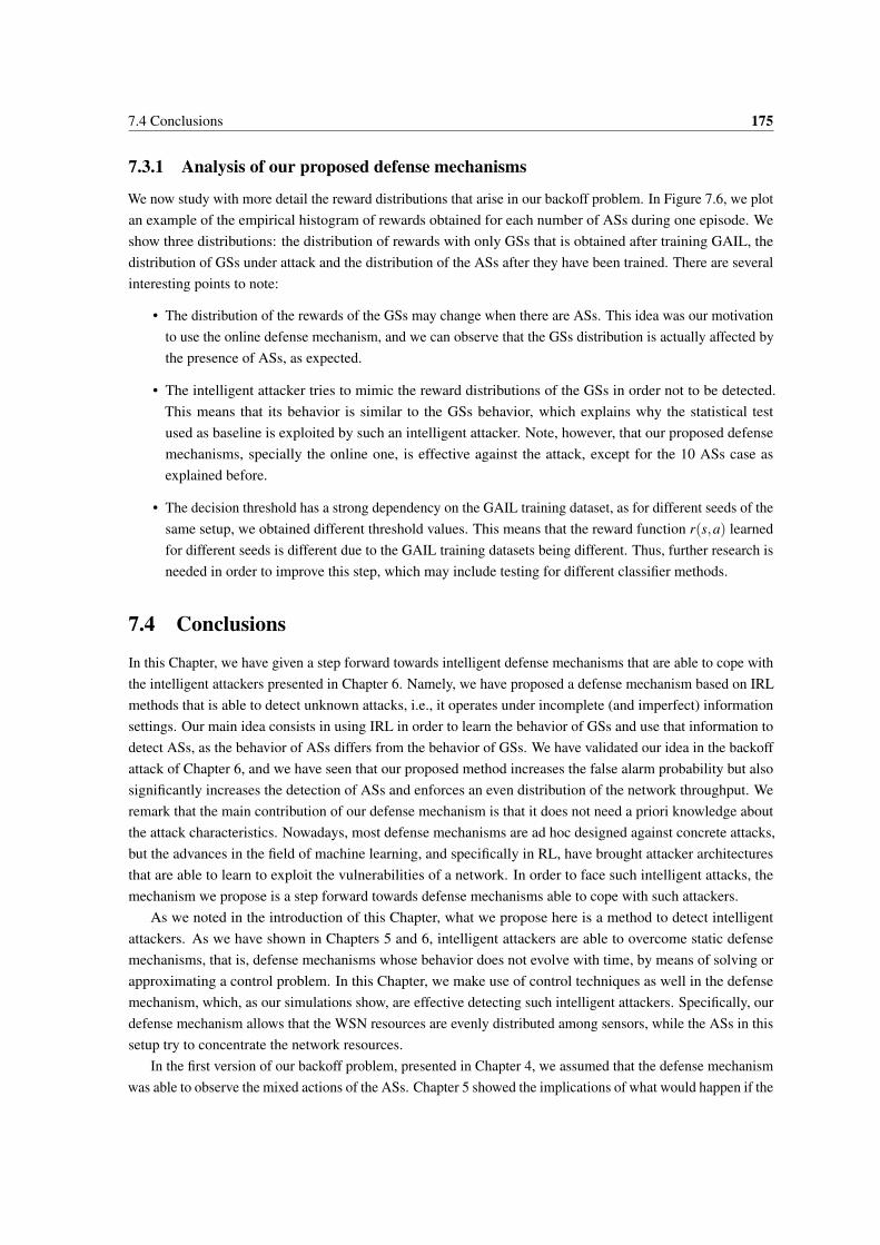
7.6 Histogram of rewards compared for GSs and ASs, for one seed. From left to right: 1/5/10ASs. Top are for offline defense, bottom for online. Peaks have been cut off for clarity. Blueis the reward histogram when only GSs are present, that is, for training, orange is for GSsunder attack and green is for ASs during attack. The red line is the decision threshold obtainedduring training. Note how sometimes, the ASs are able to behave in such a way that theymimic the reward shape of the GSs, but other times they do not. Also, note how the GSsdistribution changes if there is an attack: this explains why the online defense mechanismperforms significantly better. . . . . . . . . . . . . . . . . . . . . . . . . . . . . . . . . . . . 176

List of tables

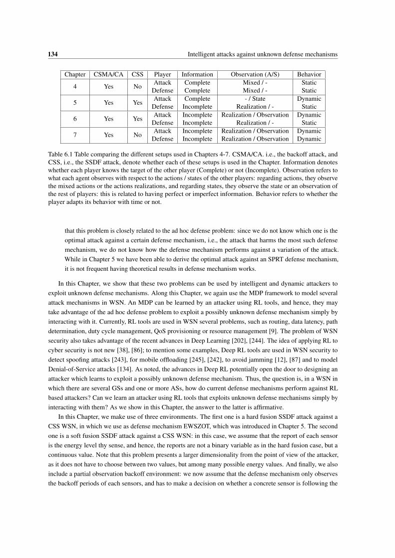
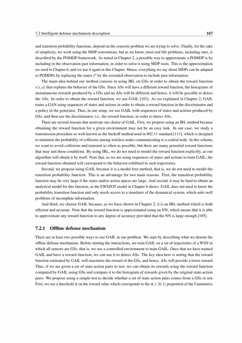
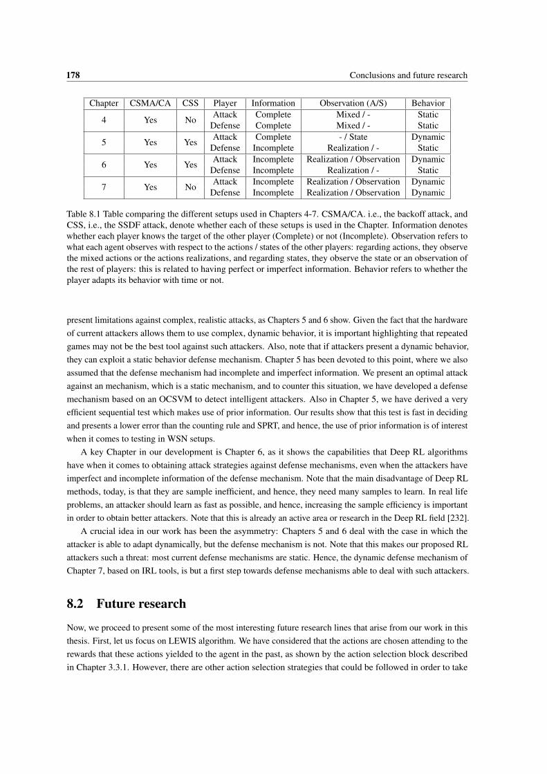
1.1 Table comparing the different setups used in Chapters 4-7. CSMA/CA. i.e., the backoff attack,and CSS, i.e., the SSDF attack, denote whether each of these setups is used in the Chapter.Information denotes whether each player knows the target of the other player (Complete) ornot (Incomplete). Observation refers to what each agent observes with respect to the actions/ states of the other players: regarding actions, they observe the mixed actions or the actionsrealizations, and regarding states, they observe the state or an observation of the rest of players:this is related to having perfect or imperfect information. Behavior refers to whether the playeradapts its behavior with time or not. . . . . . . . . . . . . . . . . . . . . . . . . . . . . . . . 4

3.1 Comparison of theoretical εi values for the Nash equilibrium concept, when using equispacedsampling, according to (3.31), where Ki = 50. In all cases, ε1 = ε2, that is, both players had thesame bound. . . . . . . . . . . . . . . . . . . . . . . . . . . . . . . . . . . . . . . . . . . . . 73


4.2 Values used for simulation 1. . . . . . . . . . . . . . . . . . . . . . . . . . . . . . . . . . . . 844.3 Payoffs values for the game posed, when n2 = 1. The payoff vectors are of the form r = (r1,r2),

where r1 is the payoff of the server and r2 is the payoff of the AS. . . . . . . . . . . . . . . . 864.4 Payoffs values for the game when n1 = 4 and n2 = 1. The first entry of the payoff vector is the

server payoff, the second is the AS payoff. . . . . . . . . . . . . . . . . . . . . . . . . . . . . 904.5 Empirical payoffs obtained using RM for each value of n2. Observe that payoffs do not

significantly vary as the number of players increase. This is consistent with Figure 4.4: thegame tends to the two player situation, even if there are more players. . . . . . . . . . . . . . 90

xxvi List of tables


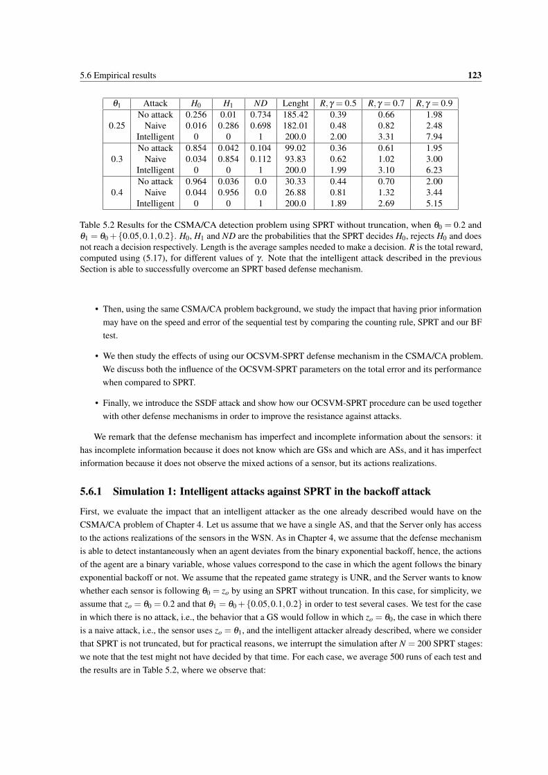
5.2 Results for the CSMA/CA detection problem using SPRT without truncation, when θ0 = 0.2and θ1 = θ0 +{0.05,0.1,0.2}. H0, H1 and ND are the probabilities that the SPRT decides H0,rejects H0 and does not reach a decision respectively. Length is the average samples needed tomake a decision. R is the total reward, computed using (5.17), for different values of γ . Notethat the intelligent attack described in the previous Section is able to successfully overcome anSPRT based defense mechanism. . . . . . . . . . . . . . . . . . . . . . . . . . . . . . . . . 123

5.3 Test results for θ0 = 0.5 and ρ = 0.05, for all the tests simulated. Each table entry is thepercentage of times that H0 was decided / H0 was rejected / no decision was taken. Observehow when facing the control law from Theorem 4, SPRT is totally unable to detect the AS.However, the exact opposite happens with our proposed SPRT-OCSVM mechanism: it alwaysdetects such an AS. . . . . . . . . . . . . . . . . . . . . . . . . . . . . . . . . . . . . . . . . 126


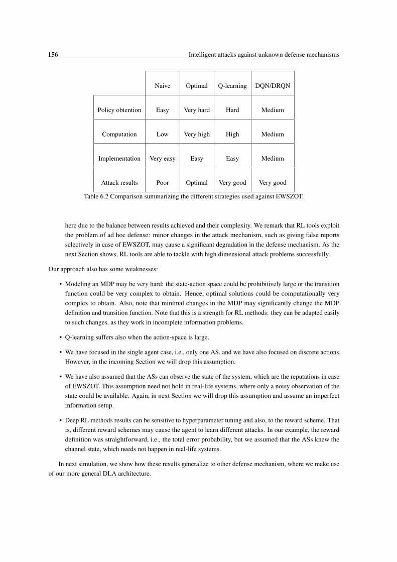
6.2 Comparison summarizing the different strategies used against EWSZOT. . . . . . . . . . . . . 1566.3 Final rewards obtained for each combination of attack, number of ASs and setup. The values

were obtained averaging 50 episodes for the best 5 seeds of each case. We show the mean finalreward, ± one standard deviation. Bold entries are the largest mean reward using DLA, wherea Welch test is used to detect whether means are significantly different for a significance levelα = 0.01. Higher is better. . . . . . . . . . . . . . . . . . . . . . . . . . . . . . . . . . . . . 161

6.4 Mean final rewards obtained for the two baselines. The values were obtained averaging 50episodes. In bold, we show when a baseline provides an equal or better reward value than thebest DLA. Higher is better. . . . . . . . . . . . . . . . . . . . . . . . . . . . . . . . . . . . . 162

List of tables xxvii


7.2 Final results obtained for each number of ASs. The values were obtained averaging 100episodes for each of the best 5 seeds after training. We show the mean final value, ± onestandard deviation. Bold entries are the values with best mean, where a Welch test is used todetect whether means are significantly different for a significance level 0.01 with respect to thebaseline. In case or total reward of the attacker, proportion of GSs banned and proportion ofbits transmitted by ASs, lower is better. In case of proportion of ASs banned and proportion ofbits transmitted by GSs, higher is better. . . . . . . . . . . . . . . . . . . . . . . . . . . . . . 173


Nomenclature

Acronyms / Abbreviations

AS Attacking Sensor

BF Bayes Factor

CA Communicate & Agree

CDF Cumulative Distribution Function

CE Correlated Equilibrium

CR Cognitive Radio

CSMA/CA Carrier Sense Multiple Access with Collision Avoidance

CSS Cooperative Spectrum Sensing

DLA Deep RL Attacker

DNN Deep Neural Network

DP Dynamic Programming

DQN Deep Q-Networks

DRQN Deep Recurrent Q-Networks

EWSZOT Enhanced Weighted Sequential Zero/One Test

FC Fusion Center

FIM Fisher Information Matrix

FNN Feedforward Neural Network

GAIL Generative Adversarial Imitation Learning

GAN Generative Adversarial Network

GS Good Sensor

GT Game Theory

xxx Nomenclature

HT Hypothesis Test

IRL Inverse Reinforcement Learning

LEWIS LEarn WIth Security

LSTM Long-Short Term Memory

MAC Medium Access Control

MAL Multi-Agent Learning

MDP Markov Decision Process

MEP Maximum Entropy Principle

MME Mean-based Mean Embedding

MSE Mean Squared Error

NE Nash Equilibrium

NNME Neural Network Mean Embedding

NN Neural Network

OCSVM One Class SVM

PE Policy Evaluation

PG Policy Gradient

PI Policy Iteration

POMDP Partially Observable Markov Decision Process

POSG Partially Observable Stochastic Game

PRNG Pseudo-Random Number Generator

RG Repeated Game

RL Reinforcement Learning

RM Regret Matching

RNN Recurrent Neural Network

SG Stochastic Game

SOO Stochastic Optimistic Optimization

SPE Subgame Perfect Equilibrium

SPRT Sequential Probability Ratio Test

SSDF Spectrum Sensing Data Falsification

Nomenclature xxxi

SVM Supporting Vector Machine

TRPO Trust Region Policy Optimization

UNR Unforgiving Nash Reversion

VI Value Iteration

WSN Wireless Sensor Network

Chapter 1

Introduction

1.1 Motivation

Our world has assisted in the last years to a spectacular development and evolution of the telecommunicationand networking technologies. We are assisting to an unprecedented increase of the services offered throughthese networks, as well as to a massive growth in the number of devices connected. This development affects toall the society, as not only businesses are obtaining new services, but also the individuals. One concept that isfrequently used to refer to this tendency in the growth of interconnected devices is the term Internet of Things,which denotes the idea of connecting as many devices as possible to the Internet network. The irruption of newapplication and devices causes that the number of interconnected devices does not stop growing.

Thus, it is not a surprise that a lot of research effort is spent in different aspects related to the Internet ofThings [133], such as network protocols [166], [254], [248], efficient implementation architectures [29], [165]or concrete applications, such as industry related ones [22] or smart cities [11]. These works show that a keyconcept related to the Internet of Things are Wireless Sensor Networks (WSNs), which are wireless networks oflow capabilities devices, known as sensors, which are designed for a specific task. The authors of [191] proposefive main types of WSNs, namely, terrestrial, underground, underwater, mobile and multimedia, and mentionthat these WSNs find applications in many different areas, such as health, smart cities, smart grid, intelligenttransportation systems, farming, remote monitoring, security and surveillance of a certain area, animal trackingor disaster management. WSNs are continuously growing, and their applications, as well as their deployment,is expected to keep on growing in the future.

However, this massive growth and evolution in WSNs has also meant that new vulnerabilities and attacksagainst WSN mechanisms arise. Note that WSNs can be the target of many attacks due to the limited capabilitiesof the sensors [72], [257]. Hence, it is not a surprise that security is one of the most active areas of researchin the field of WSN, as many recent works show: [253], [208], [244], [5], [72], [132], [199], [220]. Securityrelated topics become of utmost importance given the fact that both the number of devices interconnected andthe set of WSN applications are not expected to stop growing. However, in spite of the great effort spent in thisresearch, most of the security solutions included in communication protocols and standards used in WSN arestill at a proof-of-concept level according to [220].

A powerful mathematical framework that can be used to model and address many security issues that arisein WSN is Game Theory, which is the branch of mathematics which specializes in studying the conflict amongdifferent agents. This theory can be considered mature, with many reference works such as [76], [19], [146]

2 Introduction

or [150]. We note that the idea of applying game theory tools to security problems is not new, as there aremany works on this topic, such as [8], [193], [148], [135], [68] and [145], to mention some. However, in manycases, game theory based approaches have a limited impact, because realistic, complex models easily becomecomputationally intractable.

We also note that a field that has experienced a significant growth in the last few years is the field ofDeep Learning. As the availability of big amounts of data and the evolution of the computational poweravailable to researchers has grown, the number of advances and applications in the field has experienced asignificant increase [81]. The problem of WSN security also takes advantage of these recent advances in DeepLearning [202], [244]. A family of algorithms of special interest to us is the one known as ReinforcementLearning, which is inspired by biology and tries to make an agent interacting with a dynamical system learnthe optimal sequence of actions, that is, the sequence of actions that provides it the highest reward. A keymilestone in the field was the work in [154], in which the researchers were able to train a computer to playa set of Atari games achieving better performance than a human; after this seminal work, many others havecome that have significantly expanded the field. We note that Reinforcement Learning tools have been used insecurity settings, such as routing, data latency, path determination, duty cycle management, QoS provisioningor resource management [9].

The present thesis lies at the intersection of the three mentioned fields, as we address security problems thatarise in WSN using Game Theory and Deep Learning tools. Namely, we model security situations in whichthe attacker and/or the defense mechanism make decisions sequentially, and these decisions have an impacton whether the attack is successful or not. We start modeling our security attack problems in WSN usinggame theory tools, which provide analytical solutions in controlled environments. However, as we increase thecomplexity of the security setup, we note that game theory tools are too expensive computationally, and hence,we turn to Deep Reinforcement Learning tools in order to obtain tractable solutions to our security problems.

1.2 Thesis overview

Let us now proceed to provide an overview of the main topics studied in the thesis. In this Chapter 1, weprovide a brief motivation and introduction to the topics that will be covered in the rest of the thesis. Chapter2 is devoted to present the mathematical framework in which our thesis is based. The main topics presentedare related to the control theory and game theory fields. Control theory tries to obtain the sequence of actionsthat an agent has to follow in order to optimize a certain outcome when the agent interacts with a dynamicalsystem. This framework is a generalization of optimization theory, as the role of time is key in order to obtainoptimal control sequences. There are many possible control cases, depending on whether the agent has a perfectobservation of the state of the dynamical system or only a partial observation, and depending on whether theagent knows how the system evolves with time or not. Game theory generalizes control theory when there areseveral agents that interact among them: in this case, note that the actions of each agent affect the rest of theagents, and hence, each agent solves a control problem coupled to the rest of agents. These frameworks arepresented and discussed in depth in Chapter 2.

Chapter 3 is devoted to study a concrete setup, known as repeated games, which are of interest as a firstapproach to WSN security, as they allow taking into account the effect of time. We note here that, whenoptimizing a sequence of actions, we may consider that the outcomes obtained by the agent need to bediscounted, that is, present outcomes matter more than future ones. This makes sense in WSN setups becauseof their volatility, but surprisingly it is a case which has not been thoroughly addressed in current literature.

1.2 Thesis overview 3

Hence, in Chapter 3 we start by studying two important effects that discounting introduces in these situations,and then present two algorithms specifically designed to obtain solutions in such environments.

In Chapters 4-7, we apply the tools developed in Chapter 2 and 3 to two concrete WSN attack situations.The first one, known as backoff attack, arises in a CSMA/CA multiple access situation in which several sensorstry to communicate with a central node without colliding. A widely used mechanism that can be used in thissituation is the backoff mechanism, by which the sensors defer their transmission a certain time so that thecollision probability is minimized. However, an attacker may ignore the backoff mechanism in order to getan advantage over the rest of sensors: this situation is known as backoff attack and is the central problemthat we address in this thesis. There are several possible variations of the backoff problem, but in this workwe address three, depending on two assumptions. The first assumption is that the defense mechanism is ableto instantaneously detect when an agent deviates from a previously negotiated strategy, and the second isthat the defense mechanism is able to instantaneously detect any deviation from the backoff procedure. Bothassumptions are considered in Chapter 4; in Chapter 5 we show what happens when the first assumption isdropped, and finally, Chapters 6 and 7 deal with the case in which none of these assumptions hold. Note thatwe refer indistinctly to this case as backoff or CSMA/CA attack.

A second WSN security problem that we include consists in using a WSN in order to detect whether aspectral channel is free or it is being used to transmit. This situation is known as Cooperative Spectrum Sensing(CSS). Here, an attacker may send false channel reports in order to mislead the decision about the channel state:this attack is known as Spectrum Sensing Data Falsification (SSDF) attack. It is possible that each sensor sendsas a report a binary variable which indicates whether it senses the channel free or not: this case is known ashard fusion and is studied in Chapter 5 and 6. It is also possible that each sensor sends the energy level theymeasure: in this case, the dimensionality of the problem grows as the report now is a continuous variable. Thiscase is known as soft fusion, and is addressed in Chapter 6. We refer to these problems indistinctly as CSS orSSDF attacks.

In Chapter 4, we study the backoff attack using the two assumptions explained before. We first presentanalytical results on the impact that a backoff attack has on the network distribution of resources, and weconclude that it causes that some sensors have access to more resources than others. In order to overcomethis situation, we use Game Theory tools to model this scenario. We start by modeling the CSMA/CA gameusing static game theory, and then use dynamic game theory tools, namely, repeated games. We provideanalytical solutions for the two player cases, i.e., for the case in which we have a single attacker and the defensemechanism, and also provide algorithms to solve the games when there are more than two players, where weuse the two algorithms developed in Chapter 3.

An important assumption in the backoff attack of the Chapter 4 is that the defense mechanism is able toinstantaneously detect when an attacker deviates from a previously negotiated strategy, which in game theorylanguage is known as mixed action observability. This assumption needs not hold in real environments, so wedrop it in Chapter 5. We model this new situation using detection theory tools, both including and excludingprior information, and we assume that the agent is able to perfectly observe the state of the defense mechanismand has complete information about this defense mechanism, i.e., it knows which defense mechanism is beingused. This has very important consequences, as we are able to derive an optimal attack strategy against thedefense mechanism. To counter this attack strategy, we develop a novel detection tool that successfully detectsthe attack. The advances of this Chapter introduce significant changes in the CSMA/CA setup used in theChapter 4, which we assess empirically. We also show that the attack strategy developed in this Chapter can beused to exploit a hard fusion defense mechanism in a CSS setup.

4 Introduction

Chapter CSMA/CA CSS Player Information Observation (A/S) Behavior

4 Yes No Attack Complete Mixed / - StaticDefense Complete Mixed / - Static

5 Yes Yes Attack Complete - / State DynamicDefense Incomplete Realization / - Static

6 Yes Yes Attack Incomplete Realization / Observation DynamicDefense Incomplete Realization / - Static

7 Yes No Attack Incomplete Realization / Observation DynamicDefense Incomplete Realization / Observation Dynamic

Table 1.1 Table comparing the different setups used in Chapters 4-7. CSMA/CA. i.e., the backoff attack, andCSS, i.e., the SSDF attack, denote whether each of these setups is used in the Chapter. Information denoteswhether each player knows the target of the other player (Complete) or not (Incomplete). Observation refers towhat each agent observes with respect to the actions / states of the other players: regarding actions, they observethe mixed actions or the actions realizations, and regarding states, they observe the state or an observation ofthe rest of players: this is related to having perfect or imperfect information. Behavior refers to whether theplayer adapts its behavior with time or not.

However, the attacker in Chapter 5 had complete information of the defense mechanism, which may nothold in real environments. Hence, in Chapter 6 we drop that assumption: now the agent does not have completeinformation about the defense mechanism. Moreover, the agent does not perfectly observe the state of thedefense mechanism, but it has a partial observation of it. In this situation, we develop an attack strategy that isable to successfully exploit an unknown defense mechanism simply by interacting with it. We test our ideas inthree different setups: a hard and a soft fusion CSS environments, and also in a backoff attack, in which wedrop the second assumption, that is, that the defense mechanism is not able to instantaneously detect whichsensors are not following the prescribed backoff mechanism. Actually, our proposed attacker is a real threatagainst current WSN defense mechanisms: we show that it is able to coordinate several attackers with a partialobservation of an unknown defense mechanism and successfully exploit it.

It is important noting that Chapters 5 and 6 allowed the attacker to have a dynamic behavior, whilethe defense mechanism was considered static, that is, it did not change its behavior with time. Thus, theywere asymmetric situations between the attackers and the defense mechanism, in which they have differentcapabilities and also they do not have complete information about the other players. In Chapter 7, we breakthat asymmetry as we introduce an intelligent defense mechanism that is able to face the intelligent attackerpresented in Chapter 6, whose performance is successfully tested on the same backoff attack setup of theChapter 6.

Chapter 8, finally, draws some conclusions of the thesis and also discuss several future research lines thatcould arise from this work.

In Table 1.1, we include a summary on the different setups that we study in Chapters 4-7, in order tofacilitate the ideas of the reader. This table is repeated along the text for the sake of clarity, so that the reader isoriented regarding the concrete setup under study in each of the Chapters of the thesis.

1.2.1 Publications associated to the thesis

Most of this thesis has already been published in 5 international journals and one international conference,and we note that the rest of the thesis is currently under review for publication. We now include a list thatsummarizes these publications, ordered by Chapter:

1.2 Thesis overview 5

• In Chapter 3, we present two algorithms specifically designed for learning repeated games using adiscounted scheme. The CA algorithm, which negotiates equilibria in these situations in a fully distributedway, has been published as: Parras, J., and Zazo, S, A distributed algorithm to obtain repeated gamesequilibria with discounting, Applied Mathematics and Computation, [180], whose journal metrics for2018 are: IF: 3.092, Rank Q1 (94.685 in Mathematics: applied). The other algorithm, LEWIS, which isdesigned for learning such games in an online fashion, is currently under review as: Parras, J., & Zazo,S, Learning to play discounted repeated games with worst case bounded payoff, Journal of MachineLearning Research, whose journal metrics for 2018 are: IF: 4.091, Rank Q1 (80.224 in Computer science:artificial intelligence).

• In Chapter 4, we deeply study the backoff attack effects and model it using static and repeated gametheory tools. The effects of the attack, as well as the static game solutions, have been published as: Parras,J., & Zazo, S., Wireless Networks under a Backoff Attack: A Game Theoretical Perspective, Sensors,[175], whose journal metrics for 2018 are: IF: 3.031, Rank Q1 (76.23 in Instruments and Instrumentation).Also, the repeated game solutions presented in this Chapter have been published as: Parras, J., & Zazo,S., Repeated game analysis of a CSMA/CA network under a backoff attack, Sensors, [177], whose journalmetrics for 2018 are: IF: 3.031, Rank Q1 (76.23 in Instruments and Instrumentation).

• In Chapter 5, we present an optimal attack against a sequential test and a novel defense mechanism thatcan successfully detect such attack: these results are published as: Parras, J., & Zazo, S., Using one classSVM to counter intelligent attacks against an SPRT defense mechanism, Ad-hoc networks, [179], whosejournal metrics for 2018 are: IF: 3.490, Rank Q1 (77.097 in Computer science: information systems).We also include an efficient sequential test that can incorporate prior information, and which is shown tobe fast and accurate; it is published as: Parras, J., & Zazo, S., Sequential Bayes factor testing: a newframework for decision fusion, in the 20th International workshop on Signal processing advances inwireless communications (SPAWC), [178].

• In Chapter 6, we present a thorough mathematical study of a hard fusion CSS problem and compareseveral methods to obtain attack strategies against it; this work was published as: Parras, J., & Zazo,S., Learning attack mechanisms in Wireless Sensor Networks using Markov Decision Processes, ExpertSystems with Applications, [176], whose journal metrics for 2018 are: IF: 4.292, Rank Q1 (82.33 inComputer science: artificial intelligence, 81.70 in Engineering, electrical and electronic). The rest of theChapter 6, which includes studying the case in which there are several agents with partial observation inthe soft fusion CSS problem and the backoff attack, is currently under review as: Parras, J., Hüttenrauch,M., Zazo, S., & Neumann, G., Deep reinforcement learning for attacking wireless sensor networks, ACMTransactions on Intelligent Systems and Technology, whose journal metrics for 2018 are: IF: 2.861,Rank Q2 (63.534 in Computer science: artificial intelligence, 66.774 in Computer science: informationsystems).

• Finally, Chapter 7 is also currently under review for publication as: Parras, J., & Zazo, S., InverseReinforcement Learning: a new framework to mitigate an intelligent backoff attack, IEEE Transactionson control of Network Systems, whose journal metrics for 2018 are: IF: 4.802, Rank Q1 (81.45 inAutomation and Control systems, 92.58 in Computer Science: Information Systems).

Chapter 2

Mathematical background

2.1 Introduction

This thesis deals with security problems that arise in WSNs when sensors make decisions. The existingcommunication protocols clearly define which actions a sensor has to choose so that the network functionsproperly. However, from a security point of view, we cannot assume that all sensors will follow these procedures,as there might be sensors which intentionally deviate from the prescribed actions in order to take advantage ofthe network. We denote such intentional deviations from the actions prescribed by the communication protocolsas attacks, and the sensors that deviate are Attacking Sensors (ASs), in contrast to the Good Sensors (GSs)which are those that follow the prescribed actions. Hence, in a WSN there might be GSs and ASs, and we seekto study the impact that the actions chosen by the ASs have on the whole network.

By the own nature of WSN protocols, we need to take into account the time. The actions are taken in stages,and current actions affect the future performance of the network. Moreover, we focus only in discrete time, asmost problems in WSN can be studied under this model. As we will see, the history of actions, which is the setof past actions, plays a central role in every defense mechanism, and thus, the main objective of the ASs isnot optimizing actions in isolation, but obtaining a sequence of actions that is optimal under some criterion, asmaximizing a certain reward. As we will see, this has a deep impact on the mathematical framework needed tostudy the interactions between ASs and the network: ASs are studied using the framework of control, which isa generalization of the optimization framework which takes into account the effect of time. While optimizationoutcomes a vector of optimal values for the optimization variables, control outcomes a policy, a law that defineswhich is the optimal action for each time step. The entities that take actions in the control procedure are knownas agents: in our case, agents are either the ASs or the defense mechanism of the WSN.

Thus, we consider that WSN are dynamical systems. In each time step, a dynamical system is defined bya state which contains the information needed to optimize the actions. When an agent takes an action, thedynamical system transients to a different state with a certain probability. We present the case in which theagent has access to the state in Section 2.2. However, there are cases in which the agent only has access to anoisy or partial observation of the state: this case is presented in Section 2.3.

Control theory is used to optimize the sequence of actions of a single agent. However, this needs not bethe case in our WSN environment, as there might be more than a single AS. Note that having several ASsincreases the possible attack policies, as ASs may act coordinately in order to take an advantage of the WSN. A

8 Mathematical background

mathematical model proposed for this situation, in which we have several agents with a common objective, isthe Swarm model, which we present in Section 2.4.

Of course, it may happen that the network has a defense mechanism that tries to detect and apply coun-termeasures to the actions taken by the ASs. In this case, note that we have two kinds of agents: the ASs andthe defense mechanism, each of them having a different set of actions and different objectives. Furthermore,the outcome that each agent obtains depends not only on its own actions, but also on the actions of the restof agents. Thus, this situation gives rise to coupled control problems between the agents, and it is studied bymaking use of game theory tools, which we present in Section 2.5.

2.2 Markov Decision Processes

In order to model our dynamical system, we choose to employ the Markov Decision Process (MDP) framework,as it is a flexible, well-studied and widely used model to describe such systems [25], [26], [218]. In this Section,we introduce this model and several ways to solve it, when the transition function between states is both knownand unknown. We also introduce the inverse problem, in which we try to obtain the reward function that anagent is optimizing when we are given the policy of the agent.

2.2.1 Markov Decision Process

A Markov Decision Process (MDP) is defined as follows [25], [218]:

Definition 1 (Markov Decision Process). An MDP is a 5-tuple ⟨S,A,P,R,γ⟩ where:

• S is the state set, containing all the possible states s ∈ S of the dynamical system.

• A is the action set, containing all the possible action vectors a ∈ A that the agent can use to interact withthe dynamical system.

• P : S× S×A→ [0,1] is the transition probability function in case that the states are discrete andP : S×S×A→ [0,+∞) in case that the states are continuous, where P(sn+1|sn,an) denotes the probabilityof transitioning to state sn given that the agent is in state sn and takes action an. Note that unless explicitlyindicated, we assume discrete states. The superscript indicates the time step, where n indicates thecurrent time step and n+1 the next time step, n ∈ {0,1,2,3, ...,N−1}. We consider that P is stationary,that is, it does not depend on n.

• R : S×A→ R is the reward function, where r(sn,an) denotes the reward that the agent receives when itis in state sn and takes action an. In case that n = N, where N is the terminal time step, sN is a terminalstate of the system, there are no more actions to be taken, and r(sN) is the terminal state reward. Weassume that R is bounded and stationary.

• γ ∈ (0,1) is a discount factor, used to obtain the total reward for the agent.

In general, MDPs can be of finite or infinite horizon, depending on whether the final time N is finite ofinfinite.

In a general dynamical system, the probability of transitioning from one state to another depends on theprevious history, that is, the whole set of past states and actions. Note that the history set for time index n is:

H n ≡n

∏j=0

A j×S j, (2.1)

2.2 Markov Decision Processes 9

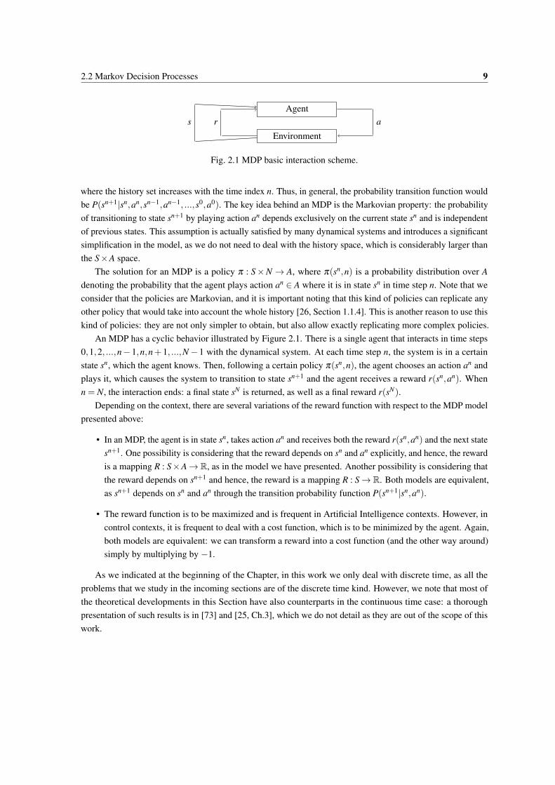
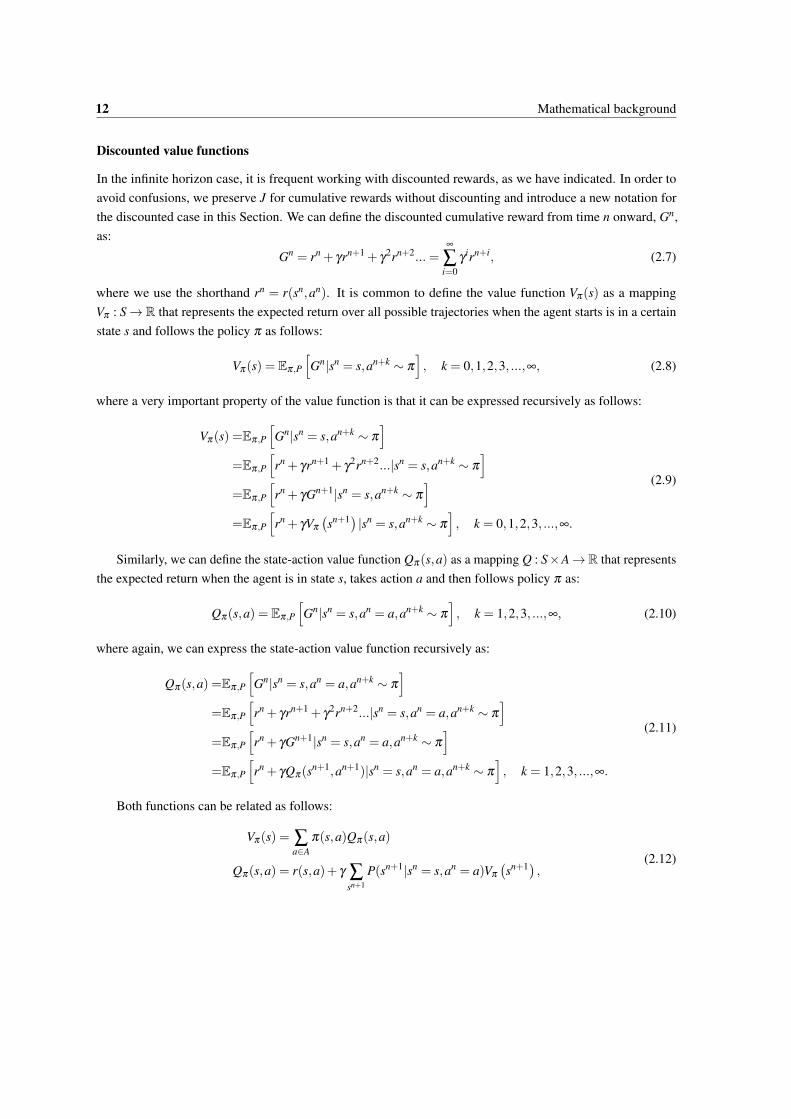
Agent

Environment

ars

Fig. 2.1 MDP basic interaction scheme.

where the history set increases with the time index n. Thus, in general, the probability transition function wouldbe P(sn+1|sn,an,sn−1,an−1, ...,s0,a0). The key idea behind an MDP is the Markovian property: the probabilityof transitioning to state sn+1 by playing action an depends exclusively on the current state sn and is independentof previous states. This assumption is actually satisfied by many dynamical systems and introduces a significantsimplification in the model, as we do not need to deal with the history space, which is considerably larger thanthe S×A space.

The solution for an MDP is a policy π : S×N → A, where π(sn,n) is a probability distribution over Adenoting the probability that the agent plays action an ∈ A where it is in state sn in time step n. Note that weconsider that the policies are Markovian, and it is important noting that this kind of policies can replicate anyother policy that would take into account the whole history [26, Section 1.1.4]. This is another reason to use thiskind of policies: they are not only simpler to obtain, but also allow exactly replicating more complex policies.

An MDP has a cyclic behavior illustrated by Figure 2.1. There is a single agent that interacts in time steps0,1,2, ...,n−1,n,n+1, ...,N−1 with the dynamical system. At each time step n, the system is in a certainstate sn, which the agent knows. Then, following a certain policy π(sn,n), the agent chooses an action an andplays it, which causes the system to transition to state sn+1 and the agent receives a reward r(sn,an). Whenn = N, the interaction ends: a final state sN is returned, as well as a final reward r(sN).

Depending on the context, there are several variations of the reward function with respect to the MDP modelpresented above:

• In an MDP, the agent is in state sn, takes action an and receives both the reward r(sn,an) and the next statesn+1. One possibility is considering that the reward depends on sn and an explicitly, and hence, the rewardis a mapping R : S×A→ R, as in the model we have presented. Another possibility is considering thatthe reward depends on sn+1 and hence, the reward is a mapping R : S→ R. Both models are equivalent,as sn+1 depends on sn and an through the transition probability function P(sn+1|sn,an).

• The reward function is to be maximized and is frequent in Artificial Intelligence contexts. However, incontrol contexts, it is frequent to deal with a cost function, which is to be minimized by the agent. Again,both models are equivalent: we can transform a reward into a cost function (and the other way around)simply by multiplying by −1.

As we indicated at the beginning of the Chapter, in this work we only deal with discrete time, as all theproblems that we study in the incoming sections are of the discrete time kind. However, we note that most ofthe theoretical developments in this Section have also counterparts in the continuous time case: a thoroughpresentation of such results is in [73] and [25, Ch.3], which we do not detail as they are out of the scope of thiswork.


2.2.2 Solving a finite horizon MDP

Let us focus in the case in which N is finite, which is known as finite horizon case. Given an initial state s0 anda given policy π(sn,n), it is possible to define the expected reward of the policy π starting at state s0, Jπ(s0), as:

Jπ(s0) = Eπ,P

[r(sN)+

N−1

∑n=0

r (sn,π(sn,n))

], (2.2)

where E denotes the mathematical expectation, which in this case is taken over the random variables sn+1 ∼P(sn+1|xn,π(sn,n)) and π(sn,n), which we recall, is a probability distribution over the action set. Hence, notethat the expected reward is strongly affected by the policy chosen, and indeed, the optimal policy π∗(sn,n) isthe one that maximizes the total reward:

Jπ∗(s0) = J∗(s0) = maxπ∈Π

Jπ(s0), (2.3)

where Π is the set of admissible policies, that is, valid distributions over actions a ∈ A, and J∗(s0) is the optimalexpected reward, which we remark, depends on the initial state s0.

A standard tool to obtain the optimal policy for an MDP is the technique known as Dynamic Programming(DP), which is owed to Bellman and that states the following [25, Proposition 1.3.1]:

Lemma 1. For every initial state s0, the optimal expected reward J∗(s0) equals the J0(s0) obtained using thefollowing backwards recursion from time step N−1 to time step 0:

JN(sN) = r(sN)

Jn(sn) = maxπ∈Π

Eπ

[r (sn,an)+ ∑

sn+1∈S

P(sn+1|sn,an)Jn+1

].

(2.4)

The optimal policy π(sn,n) can be obtained as:

JN(sN) = r(sN)

π∗(sn,n) = argmax

π∈ΠEπ

[r (sn,an)+ ∑

sn+1∈S

P(sn+1|sn,an)Jn+1

].

(2.5)

As shown by the previous Lemma, DP algorithm proceeds backwards by relying on the fact that, whenoptimizing for time step n, we have previously optimized for time steps n+1 to N. Thus, we cannot improveJn+1 as it has already been optimized in the previous iteration, and hence, we have to find the optimal action forthe current time step n. This is known as the Principle of Optimality, and according to Bertsekas, “the principleof optimality suggests that an optimal policy can be constructed in piecemeal fashion, first constructing anoptimal policy for the “tail subproblem" involving the last two stages, and continuing in this manner until anoptimal policy for the entire problem is constructed" [25, p. 19]. Note that the DP algorithm shown in Lemma 1suffers from the so called “curse of dimensionality": the algorithm scales badly with large states and actionspaces, and long horizons, as the memory and computation complexity depends on these parameters. Hence, itis no surprise that in practice, infinite horizon iterative methods, which scale better, are generally used.

The results in this Section have been established considering that the probability transition function wasstochastic. However, it is possible that P(sn+1|sn,an) is deterministic, i.e., the probability transition functionassigns all the probability to a single state sn+1 for each (sn,an) pair. In this case, the optimal policy π∗(sn,n)


may be replaced for a sequence of actions of length N: a0,a1, ...,aN−1, as the state trajectory is perfectlypredictable given s0 [25, Chapter 3]. This case is sometimes known as Open-Loop: for each initial state,the agent needs to compute an optimal action sequence and apply it, without the need to observe the statesn, n > 0, as this state is perfectly predictable. A widely used tool for such problems is the MinimumPrinciple, derived by Pontryagin [73]. In contrast with the Open-Loop situation, we do not assume in thiswork that the transition function is deterministic. Thus, the agent does need to observe the state sn in order toachieve optimality: this solution implies the use of a certain policy π(sn,n) which depends on sn. This solution,frequently known as Closed-Loop or feedback solution, can be computed using the Dynamic Programmingalgorithm just explained and will be used in the rest of this work. Note that using a Closed-Loop solution doesnot provide a loss of generality, as in the case of having a deterministic transition function, the policy obtainedby DP is optimal.

2.2.3 Solving an infinite horizon MDP

In an infinite horizon problem, we have that N = ∞, that is, that the number of time steps are infinite. In thesecases, the expected reward is defined as:

limN→∞

Eπ,P

[N−1

∑n=0

γnr (sn,π(sn,an))

], (2.6)

where we note these important differences between (2.2) and (2.6):

• In the infinite horizon problem there is no final reward associated with a final state, as there is no such afinal state due to having an infinite horizon.

• In the infinite horizon problem, there is a discount factor γ ∈ (0,1), which is used to weight how importantare future rewards. As γ < 1, future rewards matter less than the current reward from the optimizationperspective. Note that we need γ < 1 and R bounded in order to guarantee that the expected reward (2.6)exists, as it is the sum of infinite terms geometrically weighted by γn. In the finite horizon problem, notethat γ = 1, which means that all rewards matter the same from the optimization perspective. It is alsopossible to work with an average reward concept in the infinite horizon setting, but we only use it inChapter 3, where we introduce it. A detailed introduction to the average reward case is given in [26].

• The policy in the infinite horizon problem now is stationary: note that it does not depend on time.Intuitively, this is due to the fact that, each time that we are in a certain state s, there is still infinitetime steps to come, and hence, from the optimization perspective, the actual value of the time step isindifferent to the agent. Note that this is not the case in the finite horizon case, as being closer to the finaltime step N may have an influence on the optimal policy.

We here introduce some notation regarding the policy. π(a|s) is the vector of dimension A which containsthe probability distribution over the action space given the state s; that is, each entry of the vector contains theprobability of choosing each action in the state s. π(s,a) is a scalar which contains the probability of choosingaction a in state s: note that π(a|s) is formed by stacking the π(s,a) values for all possible actions in the states. And finally, we reserve π(s) to the mapping used when the policy is deterministic, where π(s) returns theaction a prescribed by the deterministic policy π for the state s.


Discounted value functions

In the infinite horizon case, it is frequent working with discounted rewards, as we have indicated. In order toavoid confusions, we preserve J for cumulative rewards without discounting and introduce a new notation forthe discounted case in this Section. We can define the discounted cumulative reward from time n onward, Gn,as:

Gn = rn + γrn+1 + γ2rn+2...=

∞

∑i=0

γirn+i, (2.7)

where we use the shorthand rn = r(sn,an). It is common to define the value function Vπ(s) as a mappingVπ : S→ R that represents the expected return over all possible trajectories when the agent starts is in a certainstate s and follows the policy π as follows:

Vπ(s) = Eπ,P

[Gn|sn = s,an+k ∼ π

], k = 0,1,2,3, ...,∞, (2.8)

where a very important property of the value function is that it can be expressed recursively as follows:

Vπ(s) =Eπ,P

[Gn|sn = s,an+k ∼ π

]=Eπ,P

[rn + γrn+1 + γ

2rn+2...|sn = s,an+k ∼ π

]=Eπ,P

[rn + γGn+1|sn = s,an+k ∼ π

]=Eπ,P

[rn + γVπ

(sn+1) |sn = s,an+k ∼ π

], k = 0,1,2,3, ...,∞.

(2.9)

Similarly, we can define the state-action value function Qπ(s,a) as a mapping Q : S×A→R that representsthe expected return when the agent is in state s, takes action a and then follows policy π as:

Qπ(s,a) = Eπ,P

[Gn|sn = s,an = a,an+k ∼ π

], k = 1,2,3, ...,∞, (2.10)

where again, we can express the state-action value function recursively as:

Qπ(s,a) =Eπ,P

[Gn|sn = s,an = a,an+k ∼ π

]=Eπ,P

[rn + γrn+1 + γ

2rn+2...|sn = s,an = a,an+k ∼ π

]=Eπ,P

[rn + γGn+1|sn = s,an = a,an+k ∼ π

]=Eπ,P

[rn + γQπ(sn+1,an+1)|sn = s,an = a,an+k ∼ π

], k = 1,2,3, ...,∞.

(2.11)

Both functions can be related as follows:

Vπ(s) = ∑a∈A

π(s,a)Qπ(s,a)

Qπ(s,a) = r(s,a)+ γ ∑sn+1

P(sn+1|sn = s,an = a)Vπ

(sn+1) , (2.12)


and this formulation is very interesting because it is possible to combine both expressions to obtain the followinglinear equation:

Vπ(s) = ∑a∈A

π(s,a)

[r(s,a)+ γ ∑

sn+1


(sn+1) ,] (2.13)

which can be expressed in matrix form as:

vπ = rπ + γPπ vπ , (2.14)

where each element is defined as follows, where |S| denotes the cardinality of the state set:

• vπ is a vector of dimension |S|, formed by stacking the value function values as follows:

vπ = (Vπ(s))s∈S . (2.15)

• rπ is a vector of dimension |S|, formed by stacking the reward values induced by the policy π as follows:

rπ =

(∑a∈A

π(s,a)r(s,a)

)s∈S

. (2.16)

• Pπ is a matrix of dimension |S|× |S|, formed by stacking the transition probabilities induced by the policyπ as follows:

Pπ =

(∑a∈A

π(s,a)P(sn+1|sn = s,an = a)

)s,sn+1∈S

. (2.17)

Note that Pπ is stochastic, as all its rows are probability vectors, i.e., the row elements sum 1 and all thematrix entries are greater than or equal to 0.

The Bellman operators

The matrix form of the value function expression (2.14) is of special interest in order to obtain a DynamicProgramming algorithm for the infinite horizon case. Note that we cannot apply the results obtained in Lemma1, as N→ ∞ and we do not have well-defined terminal states in the infinite horizon case. First, let us define thenext two mappings:

Tπ (Vπ(s)) = ∑a∈A

π(s,a)

[r(s,a)+ γ ∑

sn+1


(sn+1)]

T (Vπ∗(s)) = maxa∈A

[r(s,a)+ γ ∑

sn+1

P(sn+1|sn = s,an = a)Vπ∗(sn+1)] , (2.18)

where Tπ is the Bellman operator for the policy π and T is the optimal Bellman operator. Note that in theoptimal Bellman operator, we are evaluating for the optimal policy, i.e., the one that provides the optimal value.A very important result is collected by the next Lemma:

Lemma 2. Both Bellman operators introduced in (2.18) are contraction mappings with respect to the infinitynorm, for 0 < γ < 1.


Proof. A mapping F : X → X is a contraction mapping is the following conditions is fulfilled:

||F(x1)−F(x2)|| ≤ c||x1− x2||, 0 < c < 1, ∀x1,x2 ∈ X , (2.19)

where || || is a metric defined on the space X . Also, the infinity norm, or max-norm, is defined as ||v||∞ =

max |v| for a vector v.The proof for both Bellman operators introduced in (2.18) is similar, so we only include the Bellman

operator case. First, as the probability transition matrix Pπ is stochastic, the following is always satisfied:

||Pπ vπ ||∞ ≤ ||vπ ||∞. (2.20)

Thus, using the operator definition (2.18) and the matrix form given by (2.14), we have that:

||Tπ(v1)−Tπ(v2)||∞ = ||(rπ + γPπ v1)− (rπ + γPπ v2)||∞= ||γPπ(v1− v2)||∞≤ ||γPπ ||v1− v2||∞||∞≤ γ||v1− v2||∞.

(2.21)

The importance of the fact that Bellman operators are contraction mappings is that they converge to aunique fixed point using the Banach Fixed Point Theorem. The main results of applying this Theorem to theBellman operators are in the following Theorem [26].

Theorem 1. The following results hold for the Bellman operator Tπ for a policy π:

• There exists a unique solution vπ for the fixed point equation Tπ(v) = v.

• For any v0 ∈ R|S|, the sequence generated by vk+1 = Tπ

(vk)

converges to vπ as k→ ∞.

And the following results hold for the optimal Bellman operator T :

• There exists a unique solution vπ∗ for the fixed point equation T (v) = v.

• For any v0 ∈ R|S|, the sequence generated by vk+1 = T(vk)

converges to vπ∗ as k→ ∞.

Thus, this suggest that it is possible to obtain the optimal value function, and hence, the optimal policy, byrecursively applying the Bellman operators. Furthermore, it is possible to define equivalent Bellman operatorsfor the Q function with analogous properties, which we have not included for the sake of clarity. We now turnour attention to Value Iteration (VI) and Policy Iteration (PI), two DP algorithms for the infinite horizon case,which are derived from the convergence properties of the Bellman operators shown in Theorem 1.

Policy Iteration

One of the first implications of the convergence properties of the Bellman operators in Theorem 1 is that wecan recursively use the Bellman operator Tπ in order to evaluate the value function induced by a certain policyπ . This procedure is known as Policy Evaluation (PE) and consists in randomly initializing vπ and repeatedlyapplying the Bellman operator, until a convergence criterion is met, such as the maximum difference betweenvalue functions in two consecutive iterations is below a threshold. The procedure is summarized in Algorithm 1.


Algorithm 1 Policy Evaluation (PE) procedure. A usual convergence criterion is that the maximum differencebetween the v vector in two consecutive iterations is below a threshold.Input: S, A, π , R, P, γ

1: Initialize vπ arbitrarily2: while Convergence criterion is not met do3: for s ∈ S do4: vπ(s) = ∑a∈A π(s,a)

[r(s,a)+ γ ∑sn+1 P(sn+1|sn = s,an = a)vπ

(sn+1

)]Output: vπ

Algorithm 2 Policy iteration (PI) algorithm.

Input: S, A, R, P, γ

1: Initialize π0 arbitrarily2: Set k = 03: while Convergence criterion is not met do4: Obtain v

πk using the Policy Evaluation procedure (Algorithm 1).5: Improve the policy: πk+1(s) = argmaxa∈A r(s,a)+ γ ∑sn+1 P(sn+1|sn = s,an = a)v

πk(sn+1

)6: Set k = k+1

Output: vπk−1 , πk

Policy Iteration algorithm (PI) uses the convergence properties of the Bellman operator Tπ to obtain anoptimal policy π∗. It starts with π0, a randomly initialized policy, and in each iteration k of the algorithm, thepolicy πk is evaluated using the Policy Evaluation procedure already described in Algorithm 1 in order to obtainV

πk , and then, the policy is improved using:

πk+1(s) = argmax

a∈Ar(s,a)+ γ ∑

sn+1

P(sn+1|sn = s,an = a)Vπk(sn+1) . (2.22)

This procedure converges to the optimal policy π∗ as k→ ∞ [215]. The procedure is summarized inAlgorithm 2.

Value iteration

Value Iteration algorithm (VI) uses the convergence properties of the optimal Bellman operator T to obtainan optimal policy π∗. Instead of alternating between evaluating a value function and optimizing the policy as inPI algorithm, VI repeatedly applies the optimal Bellman operator to obtain the optimal value function, Vπ∗ , andonce that this value has been approximated, it is used to obtain the optimal policy as:

π∗(s) = argmax

a∈Ar(s,a)+ γ ∑

sn+1

P(sn+1|sn = s,an = a)Vπ∗(sn+1) , (2.23)

and again, this procedure converges to the optimal policy π∗ as k→ ∞ [215]. The procedure is summarized inAlgorithm 3. Note that PI requires a double loop: the inner loop firsts solves the Bellman equation for a givenpolicy, and then optimizes the policy, and this procedure is repeated several times. On the other hand, VI has asingle loop which is used to approximate the optimal value function, and then a single policy is obtained atthe end of the computation. Depending on the dimensions of the state and action spaces, the computationalresources and time required by each algorithm may differ, although both converge to the optimal solutions ofthe MDP.


Algorithm 3 Value iteration (VI) algorithm.

Input: S, A, R, P, γ

1: Initialize v0 arbitrarily2: Set k = 03: while Convergence criterion is not met do4: for s ∈ S do5: vk+1(s) = maxa∈A

[r(s,a)+ γ ∑sn+1 P(sn+1|sn = s,an = a)vk

(sn+1

)]6: Set k = k+17: Obtain the optimal policy: π(s) = argmaxa∈A r(s,a)+ γ ∑sn+1 P(sn+1|sn = s,an = a)vk

(sn+1

)Output: vk, π

As noted by Bertsekas [25, Chapter 7], the infinite horizon problem never holds in practice. Yet it is areasonable approximation for problems with many time steps. Also, note that we can model a finite horizonproblem under the infinite horizon perspective by simply adding an absorbing state to the state space of aninfinite horizon MDP: an absorbing state is a state such that the probability to transition to itself is 1, whichmeans that the agent cannot leave that state, regardless of its actions. Also, the policies in the infinite horizoncase are stationary, and hence, simpler than in the finite horizon case, and PI and VI iterative methods scalebetter than the method shown in Lemma 1 for large state and action spaces. All these reasons make infinitehorizon MDPs very popular in current applications, and also justify that we use infinite horizon models in therest of this work.

2.2.4 Model-free methods

So far, we have assumed that the transition probability function P was known and available to the agent for theoptimization procedure. However, this needs not be the case in real life problems, as the function P may beunknown or hard to obtain. In such cases, an MDP can still be approximately solved using the set of techniquesknown as Reinforcement Learning (RL). RL methods are biologically inspired and their basic intuition is that itis possible to learn how to act optimally in a dynamical system as the one shown in Figure 2.1 by interactingwith the system using trial and error. That is, the agent interacts with the dynamical system and stores sets oftuples containing information about each interaction, that is,

(sn,an,rn,sn+1

). This information is then used by

the agent to optimize a policy π that maximizes the expected discounted reward. A complete introduction tothe field is given in [215].

Q-learning

We now introduce Q-learning, a well-known RL algorithm [215]. The main idea of Q-learning is to storeestimates of the Q function (2.10) and update them as the agent interacts with the system. For simplicity, wenow assume that |S| and |A| are discrete, and hence, the Q values can be stored in a table of dimension S×A.Q-learning algorithm starts by initializing the Q function to any value, for instance, Q(sn,an) = 0, ∀sn ∈S, ∀an ∈ A. Then, the agent starts to repeatedly interact with the dynamical system: it observes its currentstate sn and takes action an following an ε-greedy policy:

πε−greedy(sn) =

{a∗ = argmaxan∈A Q(sn,an) with probability 1− ε

Random(an ∈ A\a∗) with probability ε, (2.24)


Algorithm 4 Q-learning algorithm. A typical convergence criterion is the maximum number of iterations.

Input: S, A, α , ε

1: Initialize Qπ(sn,an) = 0, ∀an ∈ A, ∀sn ∈ S2: while Convergence criterion is not met do3: Initialize n = 04: Set initial state s0

5: while State sn is not final do6: Obtain action an using ε-greedy policy (2.24)7: Take action an and obtain sn+1 and rn

8: Update Qπ(sn,an) using (2.25)9: Set n = n+1

10: for sn ∈ S do11: π(sn) = argmaxa∈A Qπ(sn,a)Output: π

where the idea in (2.24) is that the agent chooses to take the action a∗ that maximizes Q(sn,an) with probability1− ε and with probability ε , it takes a random action except a∗. Observe that the values of ε will regulatethe exploration-exploitation trade-off: high values of ε will cause that the agent explores the rewards thatdifferent actions give it, whereas low values of ε will cause the agent to exploit the action that gives it thehighest payoff. Note that a high exploration is desirable in order not to get stuck in poor maximum, whilea high exploitation provides larger rewards to the agent. In practice, it is common starting with a high ε toexplore often, and diminish its value as the training progresses. Even though other policies than ε-greedy arevalid for the Q-learning algorithm, we use it for its simplicity. Note that 0≤ ε ≤ 1.

When the agent takes action an, the environment transitions to a new state sn+1 and it returns an immediatereward rn to the agent. This allows updating the Q-function value for state sn and action an as follows:

Qπ(sn,an) = Qπ(sn,an)+α

(rn + γ max

aQπ(sn+1,a)−Qπ(sn,an)

), (2.25)

where α ∈ [0,1] is a parameter that controls the learning rate: low values of α means a low Q update, but highvalues of α introduce a high variance on Q values. Q-learning algorithm is summarized in Algorithm 4. Notethat there are similarities between Q-learning (Algorithm 4) and Value Iteration (Algorithm 3) due to the factthat Q-learning is a model-free implementation of VI, which relies on similar ideas: we try to approximate theoptimal value function, and then, we obtain an approximate optimal policy. Q-learning converges in the limit tothe optimal Q-function under some mild convergence conditions [215], [234].

Linear approximations

The previous Q-learning algorithm was derived under the assumption that the action and state spaces werediscrete, which allowed the Q-values to be stored in a table. However, as the number of states and/or actionsgrows, the memory required to store the table might be too expensive. Also, note that having a discrete statespace may be too restrictive in real life dynamical systems. A solution to these problems is to use functionapproximations for the value functions. A possible approach is using linear approximations, in which the valuefunction is approximated linearly using M basis functions φ as:

Qπ(s,a) =M

∑m=1

αmφm(s,a), (2.26)


where α is a vector of parameters with M entries and φm are M basis functions used to approximate the valuefunction. The algorithms that we have seen in the previous Sections can be adapted to deal with these linearapproximations [26, Chapter 6], in order to obtain the α vector that best approximates the value function. Themain advantage of using these approximations is that they allow dealing with many discrete states or evencontinuous states, and at the same time, control the problem complexity, as the optimization complexity dependson M instead of on |S|. However, the main problem with this approach is that the quality of the approximation isdirectly related to the approximation capabilities of the basis functions: if the actual value function is containedin the subspace spanned by the basis functions, then the approximation error will be small, but unluckily, this isnot often the case. Also, good approximation capabilities require carefully handcrafted basis functions. Due tothese problems, linear approximations are rarely used today. In the next Section, we introduce neural networksas universal function approximators, and afterwards, we present two RL algorithms that use their approximationcapabilities.

Feedforward Neural networks

Neural networks (NNs) are function approximators that are able to approximate functions to an arbitrary degreeof accuracy [105], [51]. In other words, NNs are universal function approximators. An NN is a layered structurecomposed by neurons [95]. A Feedforward Neural Network (FNN) is a directed architecture as seen in Figure2.2, in which the neurons of two consecutive layers are densely connected, thus these layers are sometimesknown as Dense. Each of the neurons outputs a nonlinear combination of its inputs as follows:

z = ϕ

(∑

iwi · xi +b

), (2.27)

where z is the neuron output, x its input vector, w is a vector of weights, b is a scalar bias and ϕ is the activationfunction, which usually is nonlinear. Note that each neuron receives as input a vector and outputs a single,deterministic value. Some of the most popular activation functions are:

Name ϕ(x) ϕ→(x)Rectified Linear Unit Activation (ReLU) max(0,x) [0,∞)

Sigmoid Activation (Sigm)ex

ex +1(0,1)

Hyperbolic Tangent Activation (Tanh)ex− e−x

ex + e−x (−1,1)

Linear Activation x (−∞,∞)

(2.28)

where ϕ→(x) denotes the image set of the function ϕ(x), and it is important to take into account it becausethe image of the output of an NN depends on the activation function of the neurons in the last layer. Theseactivation functions are also chosen because their gradient, needed for training the NN, can be easily computednumerically. Note that we include the linear activation for completeness.

Observing the FNN in Figure 2.2, we note that there is an input layer, an output layer, and an intermediate,hidden layer. Depending on the number of hidden layers, we can difference between shallow and Deep NeuralNetworks (DNNs), the former having no hidden layer and the latter having at least one. Even though theuniversal approximation property of the neural networks has been known for years [105], [51], the lack ofsufficient computational power for training these neural networks caused them not to be too successful. Thisradically changed as the computational power available to researchers grew: DNNs composed of many layers


x1

x2

z1

z2

Fig. 2.2 Example of feedforward neural network. Each circle represents a neuron, which combines non-linearlyits inputs following (2.27). The inputs are x1 and x2, and the outputs are z1 and z2. There is a single hiddenlayer, which has three neurons. Note how each of the outputs z is a nonlinear combination of the inputs x1 andx2.

can today be trained and many applications for DNNs began to appear [129]. Today, DNNs are used successfullyfor many complex tasks, such as object classification in images [258], human-like performance in Atari games[154] or indoor localization [230], to mention a few. The increasingly high computational power available evenmakes it feasible to use DNN in WSN deployments [181].

Training an NN means obtaining the set of weights and biases that approximates a certain function. This isusually done from data: we provide the NN with a dataset of inputs and outputs, and the weights and biasesare iteratively updated in order to minimize a loss between the NN output and the desired output given by thedataset. This update is usually done by means of the backpropagation algorithm [96], which is an application ofthe chain rule to obtain the gradients of the outputs with respect to the parameters of the neurons, i.e., weightsand biases, and then apply a first order optimization method, such as Adam [122], in order to update the weightsand biases of the NN.

Deep Q-Networks

As we have seen before, a main drawback of the Q-learning algorithm presented comes when the space setis large. In order to deal with this, and also with continuous state spaces, we have already presented linearapproximations, which however present questionable results, as the basis functions need to be handcrafted. Arecent approach takes advantage of the advances in Deep Learning and uses NNs in order to approximate thevalue function. The first algorithm that followed this approach was an adaptation of Q-learning, known as DeepQ-Networks (DQN) [153], [154].

DQN approach is based on Q-learning, thus it is similar to Algorithm 4, but under DQN, the Q-function isreplaced by a DNN, whose input is the current state sn and its output is the approximated Q-value function forevery action an ∈ A, Qπ(sn,an). Another characteristic of DQN is that it makes use of the past experience toenhance the learning process: at each time step, the experience of the agent en = (sn,an,rn,sn+1) is stored in adata set E. The set E is updated as new actions are taken by the agents and the data contained in E is used toupdate the NN multiple times. Experience replay allows a greater data efficiency and also, it allows avoidingthe correlation between consecutive samples, as the convergence of the gradient methods used to update the


Algorithm 5 Deep Q-Networks algorithm. A typical convergence criterion is the maximum number ofiterations.Input: S, A, ε

1: Initialize the Q-function Qπ(s,a) DNN, with weights θ

2: Initialize the target network, which is equal to the Q-function Qπ(s,a) DNN, with weights θtg = θ

3: Initialize replay memory E = {}4: while Convergence criterion is not met do5: Initialize n = 06: Set initial state s0

7: while State sn is not final do8: Obtain action an using ε-greedy policy (2.24)9: Take action an and obtain sn+1 and rn

10: Store en = (sn,an,rn,sn+1) in E11: for A batch of e ∈ E randomly sampled do12: Obtain B using (2.29)13: Update θ using B14: Set n = n+115: Update θtg = θ

16: for sn ∈ S do17: π(sn) = argmaxa∈A Qπ(sn,a;θ)Output: π

neural networks improves with uncorrelated samples [153]. Another feature of DQN consists on using targetnetworks: at each training epoch, the Q-learning DNN is cloned and the copy is called target network. Thetarget network is used to estimate the future Q values to update the NN during that epoch. Because targetnetworks are updated only once per epoch, that gives better convergence results and helps to avoid oscillations[154]. We denote the parameters of the Q function DNN as θ , and the target network parameter as θtg.

Every time that the Q-function DNN has to be trained, we randomly sample a set of experiences from thereplay memory E, and for each e, we build the following B value:

B(e) =

{rn for terminal sn+1

rn + γ maxa∈A Qπ(sn,a;θtg) for non-terminal sn+1 , (2.29)

where Qπ(sn,a;θtg) is the approximated Q-function value for the state sn given by the target network. Thus, foreach en vector, we train Qπ(sn,an;θ) to minimize the difference with respect to B(en). Note that this meansthat the Q-function DNN is trying to approximate the actual Q-function. Also, observe that we compute (2.29)using the target network, and use the resulting B values to update the θ weights.

An implementation of DQN can be observed in Algorithm 5. Again, we note that this Algorithm is similarto Q-learning (Algorithm 4), as DQN is a Q-learning based implementation using DNNs. The main advantagesof using DNNs is that they allow using continuous states and that they significantly reduce the memory requiredto store the Q-function, as it is now stored as a DNN. However, note that DQN is only valid for discrete actionspaces. Now, we turn our attention to a different way of using DNNs under an RL paradigm, in order to be ableto deal with continuous actions.

Trust Region Policy Optimization

DQN uses a DNN to approximate the Q value function. However, it is also possible to use a DNN to approximatethe policy function instead, and then compute the gradient of the total expected reward with respect to the


parameters of the DNN policy. This approach is denoted as policy gradient (PG), which englobes severalpopular Deep RL methods, such as Deep Deterministic Policy Gradient (DDPG) [136], Trust Region PolicyOptimization (TRPO) [197] or Proximal Policy Optimization (PPO) [198]. The objective of PG methods is tosolve the following problem:

maxω

Eπω ,P

[∞

∑n=0

γnrn

], (2.30)

where ω denotes the parameters of a DNN which is used to model the policy πω . According to the PolicyGradient Theorem [216], [206], the gradient of (2.30) has the following form:

∇ω

{Eπω ,P

[∞

∑n=0

γnrn

]}= Eπω ,P

[∞

∑n=0

γn∇ω logπω(an|sn)Aπω

(sn,an)

], (2.31)

where Aπω(sn,an) is the advantage function, used to estimate how good is action an when used in state sn.

Different algorithms obtain Aπω(sn,an) in different ways, for instance, we could use Aπω

(sn,an) = Qπ(sn,an) orAπω

(sn,an) = Qπ(sn,an)−Vπ(sn). In general, the advantage function is implemented using DNNs that estimatethe value function, similarly to the procedure used by DQN.

Even though it is possible to use first order methods, following in every step the gradient direction (2.31) inorder to approximate the maximum of (2.30), these methods usually have poor convergence properties as theydo not take into account the curvature of the policy surface parameters. In order to alleviate this, TRPO uses asecond order optimization method that does take into account information about the curvature. First, TRPOoptimizes iteratively L, a lower bound of the maximization objective (2.30):

L = Eπω ,P

[∞

∑n=0

γn πω(an|sn)

πold(an|sn)Aπω

(sn,an)

], (2.32)

where πold refers to the value of the DNN policy in the previous iteration. This gives rise to the followingoptimization problem:

maxω

Lπold (πω)

s.t. Eπold ,P [DKL (πω ||πold)]≤ δ

, (2.33)

where DKL (πω ||πold) is the Kullback-Leibler divergence between πω and πold , and δ is a threshold. In [197]there is a proof that (2.33) is a lower bound to (2.30), and hence, we can solve the latter by optimizing theformer. Intuitively, in (2.33) we optimize the policy that maximizes the expected reward, where the maximumdifference between the new policy with respect to the old one is limited by δ . This limitation is used to avoidlarge variations in the new policy, which may lead to poor policies: the new policy is bounded to lie within aregion bounded by δ .

In order to solve (2.33), the authors in [197] propose using Natural Policy Gradient, a second orderoptimization method that takes into account second order information about the KL-divergence, as it estimatesthe Fisher Information Matrix (FIM) of the policies for the optimization. However, inverting the FIM is costlywhen there are many parameters, and this is the usual case with DNNs. In order to overcome this, [197] uses aConjugate Gradient approach to efficiently solve the FIM inversion. This allows obtaining a gradient updatethat takes into account the policy space curvature. Finally, the policy parameters are updated using a line searchprocedure that ensures that the KL-divergence condition in (2.33) is satisfied.


Algorithm 6 Trust Region Policy Optimization algorithm. A typical convergence criterion is the maximumnumber of iterations.Input: δ

1: Initialize the policy network πω , with weights ω

2: Initialize the advantage function Aπω(sn,an)

3: Initialize k = 04: while Convergence criterion is not met do5: Use πk

ω to obtain a set of trajectories Ek

6: Estimate Aπk

ω(sn,an) using Ek

7: Estimate the policy gradient using (2.31)8: Estimate the KL-divergence and the FIM9: Use Conjugate Gradient to estimate the next gradient step ∆, which includes the policy gradient estimation

and the KL-divergence10: Perform line search to ensure that ∆ satisfies the restriction in (2.33), otherwise, shrink ∆

11: Update ωk+1 = ωk +∆

12: Set k = k+1Output: πk

The whole procedure of TRPO can be observed schematically in Algorithm 6. As TRPO is computationallyintensive, PPO was designed as a modification to TRPO that uses a surrogate function to alleviate the computa-tional load [198]. In spite of this problem, TRPO has shown to be a very powerful Deep RL algorithm, whichperforms very well in different sets of tasks, as [64] shows. Also, it is able to deal with continuous and discreteaction spaces [197], which provides a significant flexibility when it comes to real world dynamical systems.These two reasons motivate us to include TRPO in our research, as we will use it to work with continuousactions.

Finally, we note that the field of Deep RL is active with much research. There are many others algorithmsproposed, such as Asynchronous Advantage Actor Critic (A3C) / Advantage Actor Critic (A2C) [152], DuelingDeep Q-Networks (DDQN) [233], Actor Critic using Kronecker-Factored Trust Region (ACKTR) [240] orActor Critic with Experience Replay (ACER) [232], and the list expands day by day. We introduce here onlytwo of the most important algorithms, that we will use afterwards in our problems.

2.2.5 Inverse Reinforcement Learning

Inverse reinforcement Learning (IRL), also known as Inverse Optimal Control, is the complementary situationto RL. In RL, there is an agent trying to obtain a policy that maximizes a certain total cumulative reward, whilein IRL, an agent is given an optimal policy function or a set of samples from an optimal policy and tries to findthe reward function that explains the given policy. Thus, IRL tries to infer the reward that best explains thebehavior of an agent, usually called expert. In the seminal paper [164], the authors state two main reasons whyIRL is important: first, in RL settings is often assumed that the reward function is known, which needs not betrue in real life problems. Another application is apprenticeship learning: constructing an agent able to behavesuccessfully in a certain environment by learning from an expert [1]. Hence, IRL can be used to model anotheragent, which is the aspect that is of interest to us. We now turn to present several IRL algorithms, from less tomore complex.


Linear programming Inverse Reinforcement Learning

The simplest algorithm to solve an IRL problem is based on assuming that S and A are small, discrete spaces,and that we have access to the expert policy function π∗, which is deterministic: this means that all the transitionprobability is assigned to a single state. First, let us remind the matrix form of Bellman equation (2.14), whichcan be rearranged as follows:

vπ = rπ + γPπ vπ = (I− γPπ)−1 rπ . (2.34)

By considering that ≽ denotes a vector inequality, i.e., an inequality satisfied by all vector entries, it can beshown that a policy π∗ is optimal if and only if [164]:

(Pπ∗ −Pπ)(I− γPπ∗)−1 rπ∗ ≽ 0, ∀π = π

∗, (2.35)

which can be intuitively understood as follows. The first term indicates how much the transition probabilitieschange by using π∗ with respect to any other policy π ′. The second term is the value function for policy π∗.The product indicates which is the best action for each state: a policy is optimal if it chooses the best action foreach state, which is what the inequality checks. In other words, (2.35) finds for a policy π∗ which chooses thebest action for each state. If the inequality in (2.35) is strict, then the optimal policy is unique.

In (2.35), what we are trying to obtain is the vector of rewards rπ∗ , as we are given π∗. Note that (2.35) isan ill-posed problem, as there are infinitely many rπ∗ vectors that satisfy (2.35), including rπ∗ = 0. Hence, weneed to restrict the possible space of rπ∗ . In [164], the authors propose the following three ideas:

• Heavily penalize every deviation from the policy π∗. This can be done by maximizing the minimaldifference between each action in the optimal policy and the next best action for each state. By definingPπ∗(s) as the row of the matrix Pπ∗ corresponding to state s, where Pπ(s) represents the action prescribedby policy π in state s, the previous condition becomes:

max ∑s∈S

minπ

[(Pπ∗(s)−Pπ(s))(I− γPπ∗)

−1 rπ∗ .]

(2.36)

• Impose an additional sparsity restriction on rπ , by minimizing a norm-1 regularizer of the reward vector.The regularizer is controlled by a parameter λ ≥ 0. Note that this means that the reward obtained willhave as few nonzero entries as possible, which means that the reward obtained will be as simple aspossible.

• Limit the maximum value of the reward to a certain value rmax.

Putting these ideas together, we obtain the following Linear program:

max ∑s∈S

minπ

[(Pπ∗(s)−Pπ(s))(I− γPπ∗)

−1 rπ∗]−λ ||rπ∗ ||1

s.t. (Pπ∗ −Pπ)(I− γPπ∗)−1 rπ∗ ≽ 0, ∀π = π

∗

rmax ≽ |rπ∗ |

. (2.37)

It is possible to extend these ideas to less restricted setups. First, let us assume that we want to work with astate space S which is discrete with many states or even continuous. Similarly to (2.26), we can use a linear


approximation of the reward over a set of features mappings φ(s,a) as follows:

r(s,a) =M

∑m=1

αmφm(s,a), (2.38)

where the reward function is approximated by a linear combination of M fixed feature mappings φ : S×A→ R,and α is the weight vector of the linear approximation. Hence, we exchange finding a reward functionR : S×A→ R, which would involve using calculus of variations, for finding a set of scalar weights αm usingoptimization tools. Since the expectations are linear, the value function (2.8) becomes, using (2.38) and thevector form of the value function (2.14):

vπ(sn) =E

[M

∑m=1

αmφm(sn,π(sn))+ γ

M

∑m=1

αmφm(sn+1,π(sn+1))+ ...|π]

=M

∑m=1

E[αmφm(sn,π(sn))+ γαmφm(sn+1,π(sn+1))+ ...|π

]=

M

∑m=1

αmvm,π(sn)

, (2.39)

where vm,π is the value function for the mth basis feature. In this case, the optimality condition can be related tothe value function: a policy is optimal if the value function induced by that policy is larger or equal than thevalue function induced by any other policy:

Eπ∗,P [vπ∗(sn)]≥ Eπ,P [vπ(sn)] , ∀sn ∈ S. (2.40)

However, the optimality condition in (2.40) is impossible to check exhaustively on a large or infinite statespace. Also, as we are approximating using a basis function, it may also happen that the optimal rπ∗ cannotbe represented in the subspace spanned by the chosen basis functions. In order to address the former, [164]proposes checking (2.40) in a finite subset S0 ⊆ S. The latter is addressed by using a penalization function p(x):

p(x) =

{x if x≥ 02x if x < 0

. (2.41)

The idea behind using the penalization function (2.41) is that we try to minimize the number of statesfor which (2.40) is not satisfied, and this allows dealing with rewards outside of the subspace spanned by thechosen basis functions. Hence, the linear program that needs to be solved for this case is:

maxαm

∑sn∈S0

minπ

[p(Eπ∗,P[vπ∗(sn)]−Eπ,P[vπ(sn)])] , (2.42)

where we recall that vπ are functions of αm, as shown in (2.38) and (2.39).Finally, it is possible to define also a linear program for the case in which we do not have the expert policy

function π∗, but rather, we have a set of samples trajectories following the expert policy, ζπ∗ , which is formedby successive states and actions obtained by interacting with the MDP following the expert policy. We assumethat we also have access to a simulator of the MDP, so that we can generate trajectories ζπ for an arbitrarypolicy π . We also assume that we know the initial state of the system, s0. In this case, we can update (2.42)iteratively in order to obtain a reward function as Algorithm 7 shows [164], in which we alternate betweenoptimizing a linear program to obtain a reward function from the samples; and in the second step, we use an RLprocedure to obtain a policy that optimizes the reward function obtained previously. The linear program of the


Algorithm 7 Linear IRL using sample trajectories. A typical convergence criterion is the maximum number ofiterations.

Input: An MDP simulator, s0, φm basis functions1: Generate a random policy π0

2: Initialize k = 03: while Convergence criterion is not met do4: Simulate the MDP from s0 using the policy πk, in order to obtain a set of trajectories ζ

πk

5: Estimate vπk using (2.39) and ζ

πk

6: Obtain αkm as the solution to (2.43)

7: Use an RL procedure to obtain an updated πk+1 such that maximizes the expected return over the rewardfunction (2.38) with parameters αk

m8: Set k = k+1

Output: αkm

first step is:

maxαk

m

k

∑i=0

p(Eπ∗,P[vπ∗(sn)]−E

πk,P[vπk(sn)]), (2.43)

where we note that (2.43) corresponds to a particularization of (2.42) for the case that we have only trajectoriesfrom the policies. Note that the value functions are estimated using (2.39), as indicated before. Also, note thatwe store the trajectories that correspond a previous policy, as the optimal policy should be better than any ofthem. The penalization function was defined in (2.41), and again, it is used to penalize the violations of theoptimality conditions, which may happen due to the optimal reward vector not being contained in the subspacespanned by the basis functions used. We also note that the second step is key in the time budget needed for thisapproach, as in each iteration, a whole RL procedure needs to be done.

Thus, it is possible to use linear programming to solve the IRL problem for small and large or continuousstate spaces, and even if we do not have access to the expert policy function, but rather to trajectories obtainedwith it. However, all these methods assumed that the expert policy was optimal in all circumstances, whichneeds not be the case in real life problems, as the expert may occasionally act suboptimally. In order toaccommodate this possibility, we need to introduce the Maximum Entropy Principle (MEP), which has beenkey in recent IRL developments.

Maximum entropy principle

The Maximum Entropy Principle (MEP) is owed to Jaynes [112]. It is frequently used when we need tofit certain data to a distribution with the largest entropy. Intuitively, this means making the less possibleassumptions about the distribution. Formally, let us assume that we have a discrete variable xi, which may takeI possible values, i = 1,2, ..., I, and we do not know the probabilities of each xi, pi = P(xi). Jaynes was tryingto address the problem in which he wanted to obtain the expectation of a function f (x), which was also known:

Ex [ f (x)] =I

∑i=1

pi f (xi), (2.44)

and, as pi is a distribution, we also know that pi belong to a simplex, i.e., pi ≥ 0 and ∑i pi = 1. Clearly, this is aproblem in which we lack information if I > 2, as we only know (2.44) and that ∑i pi = 1 for I variables.

In order to address this situation, Jaynes used the concept of entropy from information theory, because itprovides a unique and unambiguous criterion to work with the amount of uncertainty that a discrete distribution


has. For Jaynes, entropy and uncertainty become synonyms, and the entropy takes the following form:

H(pi) =−I

∑i=1

pi ln(pi) . (2.45)

The key idea proposed by Jaynes is that, when trying to determine a discrete, unknown distribution pi, wemust maximize the entropy, i.e., maximize the uncertainty provided by our distribution. This means that we aretrying to find a probability distribution that minimizes the bias while agreeing with the given data, because ahigh entropy means having more uncertainty about the distribution. Thus, we have the following optimizationproblem:

maxpi

−I

∑i=1

pi ln(pi)

s.t.I

∑i=1

pi = 1

I

∑i=1

pi f (xi) = Ex [ f (x)]

, (2.46)

where pi > 0 is forced by having a logarithm in the function to be maximized. This problem can be solvedusing Lagrange multipliers, where the Lagrangian is:

L (pi,λ ,µ) =−I

∑i=1

pi ln(pi)−λ

[I

∑i=1

pi−1

]−µ

[I

∑i=1

pi f (xi)−Ex [ f (x)]

]. (2.47)

We can then obtain the gradient of (2.47) with respect to pi and solve to find a stationary point:

∇piL (pi,λ ,µ) =− ln(pi)−1−λ −µ f (xi) = 0→ pi = e−1−λ−µ f (xi). (2.48)

By computing the gradient with respect to λ , we obtain the first constrain:

∇λ L (pi,λ ,µ) =I

∑i=1

pi−1 = 0→I

∑i=1

pi = 1, (2.49)

and combining (2.48) with (2.49), we obtain:

I

∑i=1

e−1−λ−µ f (xi) = e−1−λI

∑i=1

e−µ f (xi) = 1→ pi =e−µ f (xi)

∑Ii=1 e−µ f (xi)

, (2.50)

which is the Boltzmann distribution with parameter µ . Hence, the maximum entropy distribution for the case inwhich we only know the mean of f (xi) is the Boltzmann distribution in (2.50).

Today, the MEP is used in settings in which the information provided is different from the expected value ofa function f (x). We note that the Boltzmann distribution is the maximum entropy distribution for the problem(2.46), but for different problems, where other information is available, different maximum entropy distributionsarise, as can be seen in [139].


Maximum entropy inverse reinforcement learning

The MEP already described allows us dealing with situations in which the expert policy cannot be guaranteedto be optimal in all situations. The incoming sections come from a control theory perspective, and in this field,it is frequent to deal with costs instead of with rewards. We remind that these two models are equivalent: areward function R : S×A→ R has always an equivalent cost function C : S×A→ R, where r(s,a) =−c(s,a).Thus, note that the agent seeks to maximize the reward function, or alternatively, minimize a cost function, butboth problems are equivalent. Let us start by assuming that the cost is a linear combination of M features:

c(s,a) =M

∑m=1

αmφm(s,a), (2.51)

where we approximate in the same way as in (2.38).The key idea now is to have a set of trajectories ζ , and define the empirical expected feature count φ as an

empirical average over the features φm when we have K trajectories ζ of length L as follows [262]:

φ =1

LK

K

∑k=1

L

∑l=1

M

∑m=1

αmφm

(sl ,al |(sl ,al) ∈ ζk

), (2.52)

where we note that the empirical feature count φ gives us information about how the features are distributed inour dataset. Thus, any candidate distribution P(ζ ) needs to match this expected empirical feature count, whichmeans that:

K

∑k=1

P(ζk)1L

L

∑l=1

M

∑m=1

αmφm

(sl ,al |(sl ,al) ∈ ζk

)= φ . (2.53)

As we have no more information about our distribution P(ζ ), except the fact that ∑i Pi(ζ ) = 1, we can usethe MEP to derive a candidate distribution for P(ζ ). Note that this is the same problem that we have posed in(2.46) and solved in (2.50): thus, the candidate distribution is a Boltzmann distribution of the form [262]:

Pα(ζk) =e−

1L ∑

Ll=1 ∑

Mm=1 αmφm(sl ,al |(sl ,al)∈ζk)

Z(α), Z(α) =

K

∑k=1

e−1L ∑

Ll=1 ∑

Mm=1 αmφm(sl ,al |(sl ,al)∈ζk), (2.54)

where Z(α) is the partition function. Observe that evaluating the partition function may be very hard, evenunfeasible, as it has to be done over the whole space of possible trajectories. However, this model is a first steptowards dealing with suboptimal expert trajectories in IRL. Intuitively, the Boltzmann distribution means thatthe probability associated with suboptimal trajectories decreases exponentially as their cost increases.

An important remark has to do with the dynamical nature of the problem. Note that the entropy that we aretrying to maximize is the conditional entropy, which is defined as follows for a sequence of states and actionsbetween time steps 0 and N:

H(a0:N |s0:N) = E

[− ln

(N

∏n=0

P(an|s0:N ,a0:n−1)

)], (2.55)

where there is a significant problem with the conditional entropy: it requires to condition on the entire trajectoryof states, from 0 to N. In [262], (2.54) can be applied because the transition probability is deterministic andknown, and hence, it is possible to obtain the complete state trajectory, as it is an open loop problem. However,in general, the MDP transitions are stochastic and thus, the conditional entropy is not a feasible approach. In


order to overcome the requirement of knowing the whole state sequence to compute the conditional entropy,causal entropy has been used instead [124], which is defined as follows:

H(a0:N ||s0:N) = E

[− ln

(N

∏n=0

P(an|s0:n,a0:n−1)

)], (2.56)

where the subtle but important difference between (2.55) and (2.56) is that in causal entropy, the conditioningis done exclusively on state values already known. In [261], it is shown that the maximum causal entropydistribution for the restrictions in (2.46) remains a Boltzmann distribution. The causal maximum entropyprinciple can also be extended to infinite horizon settings, where the discount factor γ would appear in thecausal entropy formula [30], [259].

Maximum causal entropy inverse reinforcement learning with nonlinear cost

Even though linear approximations are a good starting point when we want to deal with large or infinitestate spaces, as we noted in the RL discussion, they do not tend to achieve good results in practice, as theyrequire carefully handcrafted features basis functions to provide good approximations. We may ask whethernon-linear approximations could be used, such as approximations based on NNs. And indeed, it is possible togeneralize the maximum causal entropy framework to work with non-linear cost functions. Let us assume thatwe parameterize the cost function using a non-linear approximation whose parameter vector is θ . In this case,the probability distribution for the sample trajectories ζ follows again a Boltzmann distribution [71]:

Pθ (ζk) =1Z

exp(−cθ (ζk)), (2.57)

where Z is the partition function and cθ is the non-linear cost function parameterized by θ . An important costto be paid by using non-linear approximations is that the optimization problem that we have to solve now arenot linear programs anymore, although it is possible to use an iterative procedure which resembles the methodpresented for the case of using a linear approximation from sample trajectories.

Let us assume that we have a policy function, which is parameterized by a parameter vector ω . Note that thepolicy may be approximated using linear or non-linear approximations. The IRL problem involves obtaininga reward function that best explains the behavior of an expert. Thus, the expert policy π∗ should maximizethe total cumulative reward, or equivalently, minimize the total cumulative cost. This process could be doneiteratively with two main steps:

• In a first step, we update ω , so that the policy πω both maximizes the causal entropy of a set of experttrajectories, and also, minimizes the cost cθ . Thus, note that we use πω to define a policy which is similarto the expert.

• In a second step, we update θ so that the difference between the cost induced by the policy expert π∗

and the cost induced by the policy πω is maximized. In other words, we try to find a cost function thatseparates as much as possible the behaviors of π∗ and πω . We remind that a similar idea to this wasbehind (2.37): heavily penalizing the differences between the expert policy and a similar policy.

Thus, we alternatively optimize on θ and ω in order to solve our optimization problem in two steps. Notethat, when we update one parameter vector, the other remains fixed. Mathematically, this problem can be


expressed as follows [71]:

maxθ

[(min

ω−H(πω)+Eπω

[cθ (s,a)])−Eπ∗ [cθ (s,a)]

], (2.58)

where Eπ [cθ (s,a)] denotes the expected cost under policy π and, hence, it is the value function using costsinstead of rewards, and H(π) is the causal entropy of policy π .

Generative Adversarial Imitation Learning

The method just described to solve (2.58) presents an important drawback, namely, that the minimization stepis done by using an RL algorithm. The RL procedure is computationally expensive when having large stateand action spaces. In order to address this problem, [101] proposes an efficient way to solve (2.58), named asGenerative Adversarial Imitation Learning (GAIL). GAIL is an efficient IRL approach based on approximatingboth the policy and the cost function using DNNs. It assumes that the IRL problem (2.58) has a solution andproposes using a Generative Adversarial Network (GAN) [82] to efficiently solve the IRL problem.

A GAN is a generative model which trains two NNs in an adversarial fashion. The first NN is calledgenerator: it takes as input a random noise and produces an output which tries to match a certain distribution ofwhich we have only samples. The second NN is called discriminator: it takes as input a sample which mayhave been generated by the generator or may belong to the actual data distribution, and tries to distinguish theorigin of the sample. Both NNs are trained in an adversarial fashion, that is, the generator tries to improve itsgenerative properties until it is able to fool the discriminator.

In GAIL, the generator approximates a policy πω with weights ω . Thus, it takes as input a state s and outputsthe probability of using any action a ∈ A. The discriminator, on the other hand, is another NN parameterized byθ , Dθ : S×A→ [0,1]: it takes as input a (s,a) pair and outputs the probability that the input was generated bythe expert policy or πω . Note that the cost function depends on the discriminator as follows:

cθ = log(Dθ (s,a)). (2.59)

By training the GAN, GAIL obtains a saddle point (πω ,Dθ ) of the following expression:

Eπω[log(Dθ (s,a))]+Eπ∗ [log(1−Dθ (s,a))]−λH(πω), (2.60)

where λ ≥ 0. Note that (2.60) is equivalent to (2.58) with minor changes that allows an efficient implementationbased on GANs. First, a step of TRPO is used to minimize (2.60) with respect to ω: this step improves thepolicy πω towards being similar to the expert policy. The motivation behind using TRPO is that is preventsthe policy from changing too much between iterations because it restricts the maximum Kullback-Leiblerdivergence in the policies between iterations. And secondly, GAIL uses an Adam [122] step with respect to θ

in order to maximize (2.60) with respect to D, where we remark that the cost function is (2.59). Note that again,a method based on two steps is used, but now we need not solving the RL problem multiple times. Rather,using a GAN architecture allows solving the RL algorithm only once, by alternatively taking TRPO and Adamsteps, although from a convergence perspective it is recommendable training the generator several steps beforeupdating the discriminator.

GAIL presents several advantages. First, it uses NNs to approximate both the cost and policy function,which allows these functions to be very expressive. We have already indicated that a problem that ariseswhen using linear approximations is that the true reward function needs not be part of the subspace generated


by the basis functions. GAIL addresses this problem by making use of NNs, which are universal functionapproximators [105]. This means that GAIL could imitate arbitrarily complex behaviors from the expert.Second, GAIL can be used in large, even continuous, state and action spaces, as TRPO is able to deal withthem. Third, it needs not solving an RL problem multiple times in order to perform the optimization. Due tothese properties, we use GAIL in our problems when we need an IRL algorithm.

2.3 Partially Observable Markov Decision Processes

The previous discussion has assumed that the agent has access to the state in each iteration. However, in reallife problems, it is frequent that the agent only has access to a partial or noisy observation of the state. In orderto deal with this situation, the MDP framework needs to be extended to what is known as Partially ObservableMarkov Decision Process (POMDP), defined as follows [218]:

Definition 2 (Partially Observable Markov Decision Process). A POMDP is an 8-tuple ⟨S,A,O,P,R,Z,b0,γ⟩where:

• S is the state set, defined as in the MDP case.

• A is the action set, defined as in the MDP case.

• O is the observation set, containing all possible observations o ∈ O that the agent observes.

• P is the transition probability function defined as in the MDP case.

• R : S×A→ R is the reward function defined as in the MDP case.

• Z : S×O×A→ [0,1] is the observation model if O is discrete and Z : S×O×A→ [0,∞) if O iscontinuous, where Z(on+1|sn,an) is the probability of observing on+1 given that the agent is in state sn

and plays action an.

• b0 is the initial belief, an initial distribution over S that denotes the belief of the agent concerning theinitial state of the dynamical system.

• γ is a discount factor as in the MDP case.

Note that the main difference between MDPs and POMDPs is that in an MDP, the agent observes the stateof the system, but in a POMDP, the agent does not observe the state directly, but an observation related to thestate. Thus, the agent is uncertain regarding the current state of the system. This causes the POMDP frameworkto be more complex than the MDP framework, because both the transition and reward function depend onthe state, which the agent does not directly observe. Hence, the agent needs to estimate the current state ofthe system based on its previous observations and actions, and has to deal with the uncertainty derived of notknowing exactly the current state. Note that, in general, this implies that the optimal policy now depends on thewhole history of actions and observations: π(an|on,an−1,on−1, ...,a0,o0), instead of on the state only as in theMDP case. It also means that the complexity of solving POMDPs increases significantly when compared tosolving MDPs: for some special cases, it is shown to have exponential complexity [40]. The contrast regardingthe MDP case is notorious, as solving an MDP using DP is known to have a polynomial complexity [174].

A popular approach to solve a POMDP relies on the definition of a sufficient statistic known as belief[218]. This statistic is updated in each time step, and collects all the important information needed about the

2.3 Partially Observable MDP 31

history. Note that the history, by definition, is a sufficient statistic. We have the nice property that a POMDPis Markovian over the belief space. So, one approach consists in defining the belief, and in each time step,updating the belief and solving the resulting MDP using any of the techniques presented in the previous Section,replacing the state with the belief. However, as shown in [218], this approach can be computationally costlyeven in simple cases. An alternative representation consists in using Predictive State Representation [142],which tries to predict future possible trajectories of observations and actions.

There have also been many proposed algorithms to solve approximately a POMDP, such as [94], [144],[186], [93] and [192], to mention some. However, a very powerful approach has recently been proposed in [92],known as Deep Recurrent Q-Networks (DRQN). It consists in modifying the DQN algorithm in order to beable to work with the history of observations and actions, by using Recurrent Neural Networks (RNNs), whichwe proceed to introduce.

Recurrent Neural Networks

FNNs can be modified to include feedback from the past, giving way to RNNs. These are specially designedto process sequential data [81], as they are able to remember past information. The memory is achieved byupdating, as new data arrives, an internal state, which is then concatenated to the NN input. Hence, the outputnow is not only a function of the NN input data, but also a function of the state, which contains informationabout the past. One of the most popular architectures to implement an RNN is the Long-Short Term Memory(LSTM) architecture [104]. In an LSTM, there is a cell state cn that is updated using the data input xn and theoutput of the LSTM, denoted by yn. The superscript n is used to denote the time index. An LSTM is formed byfour different NNs, with weights wi and biases bi, i ∈ {1,2,3,4} (2.27). These four NNs are used to update yn

and cn as follows:

• First, cn is updated with the following expression:

cn = Sigm(w1 · [xn,yn−1]+b1

)· cn−1 +Sigm

(w2 · [xn,yn−1]+b2

)·Tanh

(w3 · [xn,yn−1]+b3

), (2.61)

where Sigm denotes the sigmoid function, Tanh the hyperbolic tangent function and [a,b] the concate-nation of the vectors a and b. Note that the cell state cn is updated using the previous cell state cn−1,the previous LSTM output yn−1 and the current input xn. The first term in (2.61) is called the forgetterm: the sigmoid function outputs a nonlinear combination of the current input and previous output inthe range (0,1). By multiplying this term element-wise with the previous cell state, we are determiningwhich elements from the previous cell state are forgotten.

The second term in (2.61) intuitively controls what new information we are adding to the cell state. Notethat the hyperbolic tangent term could be considered the new information that the LSTM wants to add tothe cell state, whereas the sigmoid term controls again how much of that information will be added to thecell state. Thus, the cell state update consists of two main terms: the first controls how much informationfrom the previous state cell is remembered, and the second how much information from the current inputand previous output we are adding to the state cell to remember in the next time steps.

• Second, we obtain the output to the LSTM using the following expression:

yn = Sigm(w4 · [xn,yn−1]+b4

)·Tanh(cn) , (2.62)


x1

y1

c1

x2

y2

c2

x3

y3

LSTM LSTM LSTM

c0

y0

Fig. 2.3 Illustration of the procedure of an LSTM for three time steps. The output yn is updated in each timestep using (2.62) and the cell state cn is updated using (2.61). The LSTM block is composed of four neuralnetworks, which are the same for all time steps. Note that, in the first time step, it is necessary to provide aninitial c0 and y0 in order to obtain c1 and y1.

where the input depends on the current input and cell state, and the previous output. Note that the cellstate is updated using (2.61) prior to obtaining the LSTM output using (2.62). In addition, note that(2.62) shows that the output is a filtered version of the current cell state.

It is important to note that, in each time step, the weights and biases of the four NNs that compose theLSTM architecture are the same. The training of RNNs is different from FNNs, as now the time needs to betaken into account as well, and a modified algorithm known as backpropagation through time is used [235].This algorithm computes the gradient for the weights and biases, not only taking into account the current timestep, but also the previous ones, unrolling the LSTM similarly as shown in Figure 2.3. Thus, sequences of inputdata are used for training an LSTM.

If FNNs were able to approximate any function, RNNs are able to approximate any Turing machine [205],which makes them suitable for modeling dynamical systems. The main problem with RNNs is that thesenetworks are hard to train, hence, there has been a significant effort addressed to alleviate this problem [214].Nowadays, the main architecture used to implement an RNN is the LSTM already presented, although otherstructures, such as Gated Recurrent Unit (GRU), have been proposed recently [42], however, their advantagesover LSTM are not clear [85].

Deep Recurrent Q-Networks

After DQN came out, there were several algorithms that proposed changes in the original DQN algorithm inorder to adapt it to other environments. A very interesting one is based on Deep Recurrent Q-Networks [92]. Itconsists on using DQN algorithm with a recurrent NN, namely an LSTM, to approximate the Q function. Themain intuition behind this approach is that RNNs allow taking into account the past information, and hence,they take into account the whole history. To put it differently, the RNN internal state is used to store the pastinformation, and hence, it is similar to the belief concept. As shown by [92], DRQN can successfully solvePOMDPs with many states and actions, and due to being based on DQN, it works with continuous state spacesand discrete actions. This work then was applied in many Deep RL algorithm using RNNs in order to betteraddress the partial observation that arises in many problems.

2.4 Swarms 33

However, as we noted before, the main problem with using RNNs is that they can be significantly hard totrain. Thus, today there are two main ways to approximate a POMDP by using Deep RL tools, both of whichare used in this work and in current literature:

1. Using Recurrent Neural Networks (RNNs), which are able to store past information as we have explained.This solution provides a better approximation at the cost of having a significantly larger computationalcost and a more difficult training process.

2. Using a finite vector of past observations as input to an MDP Deep RL method. In other words, we useas state a truncated history vector, where we include past information so that the Deep RL method maytake it into account. As [92] shows, this solution is an approximation for solving POMDPs, but it canprovide very good results [154].

2.4 Swarms

Until this point, we have assumed that we have a single agent interacting with a dynamical system, which mayhave either a perfect knowledge of the state or a partial observation. Now, in this section, we turn our attentionto the case in which we have more than one agent, but all of them share the same reward function. This is afirst step that allows solving the situation in which there are several agents cooperating among them to reach acommon goal, while we reserve the more general case in which we have several agents with different intereststo the next Section.

Of special interest is the concept of swarm, which is a group of agents which cooperate among them toobtain a common goal in a decentralized fashion. Swarms are inspired by nature, in which small insects areable to cooperate among them to obtain a desired objective that they could not have obtained otherwise. Forinstance, several ants cooperate to carry a burden that a single ant could not take. Hence, a swarm is a multiagent system, where each agent is simple but by means of cooperation, the system can achieve complex goals.This problem, as we will see, can be modeled under the distributed control perspective: there is a single rewardfunction to be optimized and the action vector has as components the individual actions of several agents.

2.4.1 Dec-POMDP

A first model that allows dealing with many agents and a single reward is the Decentralized Partially ObservableMarkov Decision Process (Dec-POMDP), a multi-agent model defined as follows [24], [236, Ch. 15], [173]:

Definition 3 (Decentralized POMDP). A Dec-POMDP is a 9-tuple ⟨Np,S,A,O,P,R,Z,b0,γ⟩ where:

• Np is the index set of the agents, where the subscript i = 1,2, ...,Np indexes each of the Np agents.


• A is the action set. Each agent i has its own action set Ai and A , A1×A2× ...×ANp is the productof the action spaces of each player. The joint action a = (a1,a2, ...,aNp) ∈ A is a vector formed by theactions of all agents.

• O is the observation set. Each agent i has its own observation set Oi and O , O1×O2× ...×ONp isthe product of the observation spaces of each player. The joint observation o = (o1,o2, ...,oNp) ∈ O is avector formed by the observations of all agents.


• P is the transition probability function defined as in the MDP case. Note that P depends on a, the jointaction vector.

• R is the reward function defined as in the MDP case. Note that R depends on the joint action vector a.

• Z is the observation model, defined as in the POMDP case. Note that Z uses the joint action andobservation vectors a and o respectively.

• b0 is the initial belief as in the POMDP case.


Observe that we use subindexes for agents and superindexes for time. Note that a Dec-POMDP generalizesthe POMDP framework to a multi agent setting with a common goal, because there is a single reward functioncommon to all agents. Hence, it is a convenient model for swarms. However, this is a model very hard to solve:in the best case, they are NEXP-hard, while MDPs are P-hard and POMDPs PSPACE-hard [24]. This meansthat MDPs can be solved in polinomial time, POMDPSs using a Turing machine with polynomial amountof memory and Dec-POMDPs could be solved by a Turing machine in exponential time. However, in theworst case, POMDPs are NEXP-complete, which are the hardest problems in the NEXP class. Hence, havingseveral agents comes at the cost of a significant increase in the problem complexity and tractability. Thereare several algorithms proposed for solving Dec-POMDPs, some of them based in value functions like [173]and a more recent and efficient algorithm was proposed in [61]. Even though the algorithm in [61] surpassesits predecessors, it works in very limited time horizons. Hence, the main drawback of Dec-POMDPs liesin the complexity associated to solving them. We note that, as Dec-POMDP is a model that generalizes thePOMDP model, there exists also a Dec-MDP model [24], which generalizes MDP. Dec-MDP model is similarto Dec-POMDP model except that the agents observe the state directly. As we do not use them in our problems,we do not introduce them.

2.4.2 swarMDP

In order to alleviate the complexity in the Dec-POMDP model, a particularization of this framework for swarmshas been proposed in [211]. The model proposed is known as swarMDP:

Definition 4 (swarMDP). A swarMDP is defined in two steps. First, we define a prototype A= ⟨S,A,O,π⟩,where A is an instance of each agent of the swarm and where:

• S is the set of local states.

• A is the set of local actions.

• O is the set of local observations.

• π is the local policy.

A swarMDP is a 7-tuple ⟨Np,A,P,R,Z,γ⟩ where:

• Np is the index set of the agents as in the Dec-POMDP case.

• A is the agent prototype defined before.

2.4 Swarms 35

• P is the transition probability function defined as in the MDP case. Note that P depends on a =

(a1,a2, ...,aNp), the joint action vector, as in the Dec-POMDP case.

• R is the reward function defined as in the MDP case. Note that R depends on a = (a1,a2, ...,aNp), thejoint action vector, as in the Dec-POMDP case.

• Z is the observation model, defined as in the POMDP case. Note that Z uses a = (a1,a2, ...,aNp), thejoint action vector, and o = (o1,o2, ...,oNp), the joint observation vector, as in the Dec-POMDP case.


Note that the main difference between the swarMDP and the Dec-POMDP model lies in the fact that theswarMDP explicitly makes all agents equal: they share the same set of local states, actions, observations andpolicies. Whereas under the Dec-POMDP model each agent could have a different action and/or observationset, under the swarMDP model all agents share the same local states, actions, observations and policy. Due tothis characteristic, which is called the homogeneity property, the agents are interchangeable. Also, note that asingle agent swarMDP reduces to a POMDP.

2.4.3 Mean embeddings

The homogeneity property simplifies the problem of learning under the swarMDP model, as the order of theagents does not matter to the learning process because they are interchangeable. Note that all agents sharethe same policy due to the homogeneity property, which means that each agent would act similarly as theothers if they observed the same observation on. Thus, we can use single agent Deep RL algorithms and acentralized training/decentralized execution method to find a policy that maximizes the cumulative reward[110]. For instance, we could use TRPO and train a single policy πω for all agents, which takes as input thelocal observation of each agent i ∈ Np, on

i and outputs a local action ani for time step n. During training, the

local observations of each agent are sent to the central learning algorithm for training. During execution, eachagent uses a copy of the learned policy with their own local observation. Note that, as agents do not observe thestate because we are in a partial observation environment, we either need to use a recurrent NN for the policyπω or include in the observation enough information about the past, as explained in the POMDP Section.

We finally note that the observation vector of agent i may include not only information about agent i, butalso information about other agents if the agents are able to communicate. Let us denote by on

i,i the informationavailable to agent i about itself in time n, and on

i, j the information available to agent i about agent j, j = i.A naive way of encoding this information is to build the total observation vector of agent i, on

i by simplyconcatenating on

i,i and all the vectors oni, j. However, this concatenation causes a large input space, as well as

ignoring the permutation invariance inherent to a homogeneous swarm. A better option consists in using meanembeddings [209], [110]. There are several possible mean embeddings that can be used:

• Neural Networks Mean Embedding (NNME): In this approach, each oni, j is used as input to an NN,

which outputs φ(oni, j), where φ denotes the transformation done by the NN. The total observation vector

of agent i, oni , is built by concatenating on

i,i to the mean of all φ(oni, j). That is, we obtain the features

using the NN first, and use the averaged value of such features as input to the policy. A very interestingcharacteristic of this approach is that it allows training the mean embedding NN together with the policy,and hence, this NN will be trained to extract the information that the policy needs, thus being able toadapt to a concrete problem setup.


• Mean-based Mean Embeddings (MME): Under this approach, we average oni, j and concatenate it to on

i,i.This vector is the input to the policy network. Note that this case is a simpler approach, in which we donot perform any feature extraction process and which does not adapt to a concrete setting. Its successwill strongly depend on how informative the average values of the observation vectors are for the policy.

Note that mean embeddings are thus insensitive to the number of agents to which each agent i can communicateand is also insensitive to their order. We remark that this tool allows us to solve swarMDP problems by makinguse of the single agent methods presented in previous Sections.

2.5 Game theory

In this section, we turn our attention to the case in which there are several agents, each of them with possiblydifferent reward functions. That is, each agent may have different interests, and the actions that each of themchooses affect the rewards of the rest of the players. The branch of mathematics that studies this problem isGame Theory (GT). Currently, GT is a mature field with many important works covering different aspects ofthe theory, such as [76], [19], [146] or [150]. Closely related to this field is the field of Multi-Agent Learning(MAL), which seeks to find optimal policies for agents that are interacting with others. Even though it ispossible to pose the MAL problem from the GT perspective [204], we note that MAL can be studied usingother tools than game theory ones [213].

In this Section, we start by presenting the simple case in which the agents interact a single time, known asstatic game. We then move on to study the case in which the agents interact repeatedly over time, introducingthree models that take into account the time, with different complexities: repeated games, stochastic gamesand partially observable stochastic games. And finally, we introduce the concepts of imperfect and incompleteinformation, which will be of capital interest in the incoming Chapters.

2.5.1 Static games

We start studying the case in which the agents interact a single time. We introduce minor notations changesregarding the previous Sections: an agent may be called also a player, and the reward function may be calledalso outcome or payoff. Keeping that in mind, a static game is defined as follows:

Definition 5 (Static game). A static game is a 3-tuple ⟨Np,A,r⟩, where:

• Np denotes the number of players, where the subscript i = 1,2, ...,Np indexes each of the Np players.

• A is the action set. Each player i has its own action set Ai and A , A1×A2× ...×ANp is the productof the action spaces of each player. The joint action a = (a1,a2, ...,aNp) ∈ A is a vector formed by theactions of all players.

• r is a continuous function that gives the game payoffs as:

r : A→ RNp (2.63)

where ri(ai,a−i) denotes the payoff or reward obtained by player i when she plays action ai and the restof the players play a−i, where the index −i is a shorthand for all players except i.

In this Section, we consider discrete sets of actions. Hence, the payoff functions will be also discrete.If an action set is discrete, each of its components is denoted as pure action. Mixed actions are distribution

2.5 Game Theory 37

probabilities for each player that map each pure action of the player with the probability that the player playsthat action.

Observe that the payoff functions denote the nature of the game. It can be purely competitive: the gains ofsome players are the losses of the others and thus, ∑i ri = 0, which is the case known as zero-sum game. Itcan be purely cooperative if all players share the same payoff function. It can finally range between these twoextreme cases: these games are known as general-sum or nonzero sum games.

Nash equilibrium concept

We note here that static games can be seen as a generalization of the optimization field, in which we haveseveral agents trying to maximize their reward. However, now it is possible that, as the interest of agents maybe in conflict, they are not able to attain their maximum reward, and a different solution concept is needed forgames: the concept of equilibrium. There are several equilibrium notions, and in this work, we introduce twoof them: the Nash Equilibrium (NE), and the Correlated Equilibrium (CE).

A Nash equilibrium (NE) [161] of an Np-player game is an action vector such that no player can gain bydeviating unilaterally. Mathematically, for a static game, an action vector a is a Nash εi-equilibrium of thegame G, where εi ≥ 0,∀i ∈ Np if:

ri(ai,a−i)≥ ri(a′i,a−i)− εi, ∀i,∀a′i = ai, (2.64)

where ai denotes the possibly mixed action of player i and A−i the action of all players but player i. Whenεi = 0,∀i, we have an NE. A nonzero sum game is guaranteed to have at least one NE in mixed actions [19],which assumes that each player has access to a randomizing device which outputs which action the playershould play with a given probability. This probability is the mixed NE. In general, nonzero sum games maybecome hard to solve and might have more than one NE [19, Ch. 3]. A general review on these games and thedifferent algorithms proposed for finding equilibria can be found in [149].

We now restrict our NE analysis to the two player case, and the literature shows that this is still an area ofresearch. In [226] there are some methods used to compute two player NE, and in [16], the authors present twodifferent methods to derive all the NE in a two player game. From here on, we focus on the concrete case thatNp = 2 and both players can choose between two possible actions. Hence, the payoff function for each playermight be represented using a 2×2 matrix, and that is the reason these games are sometimes known as bimatrixgames. If we denote the payoff matrix for player 1 as R1 and R2 for player 2, we have:

R1 =

(r1,11 r1,12

r1,21 r1,22

)R2 =

(r2,11 r2,12

r2,21 r2,22

), (2.65)

where ra,bc denotes the reward that player a receives when player 1 plays her action b and player 2 plays heraction c. Hence, note that we consider that the row player is the player 1, while the player 2 is the columnplayer. As the payoffs contained in these matrices are rewards, each player tries to maximize her own payoff.As mentioned in (2.64), if we only take into account pure actions, the payoffs (r1, j∗k∗ ,r2, j∗k∗) in pure actionsNE must satisfy the following conditions:

r1, j∗k∗ ≥ r1, jk∗

r2, j∗k∗ ≥ r2, j∗k, (2.66)


where j and k index the actions of player 1 and 2 respectively. The existence of a pure action NE depends onthe reward matrices, and note that such NE needs not exist. However, we know that there exist at least a mixedactions NE. Let us define y as the probability that player 1 chooses her action 1, and 1− y the probability thatshe chooses action 2; and for player 2, we define in an equivalent form z and 1− z. It is possible to refer to y asthe mixed action of player 1, and z as the mixed action of player 2. Using this, the conditions in (2.66) can beexpressed as follows:

(y∗v)T R1z∗v ≥ yT

v R1z∗v

(y∗v)T R2z∗v ≥ (y∗v)

T R2zv, (2.67)

where yv = (y,1− y), zv = (z,1− z) and yTv denotes the transposed of vector yv. In both (2.66) and (2.67) it

is assumed that both players are maximizers: otherwise, the inequality should be reversed. The system ofinequalities in (2.67) can be solved as shown in [19, pp. 85-87] and, by using the expressions in (2.65), it yieldsthe following values for an NE:

y∗ =r2,22− r2,21

r2,11 + r2,22− r2,21− r2,12

z∗ =r1,22− r1,12

r1,11 + r1,22− r1,21− r1,12

, (2.68)

where these expressions yield a valid solution if y∗ ∈ [0,1] and z∗ ∈ [0,1]. These expressions are the samewhether the players are minimizing or maximizing. It is interesting noting that each player optimizes onlytaking into account the other player’s payoff matrix.

A final consideration on (2.68) arises when the denominator becomes null, that is, either r2,11 + r2,22−r2,21− r2,12 = 0 or r1,11 + r1,22− r1,21− r1,12 = 0. Substituting these conditions in (2.67) shows that the NEwill be in pure actions, as y,z ∈ {0,1}, which means that all the probability is assigned to one of the actionsthat a player can choose.

Correlated equilibrium concept

The CE concept, owed to Aumann [13], generalizes the NE concept. The CE is based on the possibilitythat players might communicate and coordinate themselves. It assumes that there is a correlating device thatproduces a signal sent to all players. They use this signal in order to coordinate and obtaining a higher rewardthan if they did not coordinate. Each signal of the correlating device corresponds to a pure action for eachplayer. The CE is defined so that no player has any advantage if she deviates from the prescription of thecorrelating device. More formally, a CE for Np players is defined as a distribution probability φ(a) over theset of joint pure actions of the players A = A1×A2× ...×ANp , where a = (a1,a2, ...,aNp) is a vector of pureactions such that a ∈ A. The equilibrium condition that must be satisfied for every player i ∈ Np is [13] [76]:

∑a∈A

φ(a)ri(ai,a−i)≥ ∑a∈A

φ(a)ri(a′i,a−i)− εi, ∀a′i ∈ Ai, ai = a′i, (2.69)

where the distribution φ is the εi-CE of the game. For εi = 0,∀i, we have a CE. The signal that coordinates theplayers follows the distribution φ(a) and the equilibrium is reached if no player has an advantage by deviating.

2.5 Game Theory 39

An equivalent way of expressing (2.69) is found in [76] and is the following, for εi = 0:

∑a−i∈A−i

φ(a−i|ai)ri(ai,a−i)≥ ∑a−i∈A−i

φ(a−i|ai)ri(a′i,a−i), ∀a′i ∈ Ai, ai = a′i, (2.70)

where A−i is the set of joint pure actions of all players except player i. This way of expressing a CE highlightsthat it is not profitable for player i to deviate, if every other player follows the action prescribed by the correlatingdevice.

CE are a generalization of NE: every NE will have an equivalent CE, but not all CE have an equivalent NE.However, CE are significantly less expensive to compute than NE, as it is shown in [79] and [80]. In general,CE yield a region of valid equilibrium payoffs, as a function of the distribution φ(a). Hence, the problem ofselecting an equilibrium point arises, as in the NE case. This problem is known as bargaining in literature andthere are different mechanisms proposed for equilibrium selection, as the Nash bargaining solution [160], theKalai-Smodorinsky solution [118] or the egalitarian solution [117].

Regret Matching

The Regret Matching (RM) algorithm, proposed by Hart and Mas-Colell [90] [91], is an algorithm which isused to learn the CE of a game by playing it several times. The players adapt their strategy in such a way thatguarantees that the joint distribution of play converges to the set of CE of the underlying game if each playerplays a regret matching strategy [91].

The rule that governs how a player plays according to an RM strategy is: “switch next period to a differentaction with a probability that is proportional to the regret for that action, where regret is defined as the incrementin the payoff had such a change always been made in the past" [91]. Hence, the main idea is to keep and updatea regret measure for each player, which is a vector with as many components as the number of pure actionsof the player. The game is played repeatedly over time, and each player updates his regret depending on theoutcome they obtain each time they play. This algorithm requires that player i knows the actions of all players,as well as her payoff function, but note that player i needs not knowing the payoff functions of the rest of theplayers. The regret that each player has after playing is the difference between the payoff they would haveobtained if they had played differently and what they actually obtained. In each iteration, the regret Wi(a′i) isobtained as:

Wi(a′i) = ri(a′i,a−i)− ri(ai,a−i), ∀a′i ∈ Ai, (2.71)

where ai is the pure action played by player i, a′i is used to denote all pure actions available to player i and Ai isthe set of pure actions for player i. Obviously, the regret of playing action ai is 0. If the regret of an action ispositive, RM will assign positive probability to that action to be played, because the player would have gainedin the past if she had used this action. On the other hand, if the regret of an action is negative, the player willassign probability 0 to that action, as the player would not have improved her payoff by using that action in thepast and hence, she will not use it. At the beginning of the game, the regrets are initialized to 0, and they areupdated with each repetition of the static game following:

W n+1i (a′i) =W n

i (a′i)+Wi(a′i), ∀a′i ∈ Ai, (2.72)

where W ni (a

′i) is the regret at the beginning of the previous iteration n and Wi(a′i) is obtained using (2.71).

At the beginning of each time step n, each player chooses a pure action randomly following a distribution


pi(a j), where pi(a j) is the probability that player i uses pure action a j. The probability pi(a j) is obtained atthe beginning of each time step as follows:

• If all regrets are less or equal than zero, then choose a pure action randomly following the uniformdistribution pi(a j):

pi(a j) =1|Ai|

(2.73)

where |Ai| stands for the number of pure actions available to player i.

• If there are regrets strictly higher than zero, then choose a pure action randomly following this distributionpi(ai):

pi(a j) =

{W n

i (a j)W if W n

i (a j)> 00 if W n

i (a j)≤ 0(2.74)

whereW = ∑

a j∈Ai|W ni (a j)>0

W ni (a j) (2.75)

that is, W is the sum of all positive regrets in time step n. Observe that W is computed in each timestep, as the vector W n

i is updated in each time step. This definition of W guarantees that the distributionin (2.74) adds up to 1 and has nonnegative components, which are the two requisites to have an actualdistribution.

2.5.2 Repeated games

The simplest way of taking time into account in game theory consists in playing a static game several timessequentially. This is the simplest dynamic game, known as Repeated Game (RG) [76], [146]. Formally, an RGis built using a static game, which is played repeatedly over N periods. This static game is called stage game.In an RG, the stage game is played on the periods n ∈ {0,1,2, ...,N−1}. We consider only RGs of infinitehorizon, that is, N = ∞. We define an RG as:

Definition 6 (Repeated game). An RG is a 6-tuple ⟨Np,A,r,σ ,H t ,γ⟩ where:

• Np,A and r are defined as in the static game.

• H n denotes the set of histories. A history hn ∈H n is a list of n-action profiles played in periods{0,1, ...,n−1}.

• A strategy for player i is a mapping from the set of all possible histories into the set of actions: σi : H →Ai.

• The average discounted payoff to player i, is given by:

Vi(σ) = (1− γ)∞

∑n=0

γnrn

i (σi,σ−i), (2.76)

where γ ∈ (0,1) is the discount factor. In case of having mixed actions, the average discounted payoff iscomputed taking expectations.

We focus on RGs of perfect monitoring [146]: the history hn is known to all players. In case of mixedactions, this means that the output of the randomizing device of each player is also observed by other players

2.5 Game Theory 41

[4]. Note that payoff is normalized with the term 1− γ , which allows comparing payoffs in the RG with theones in the stage game. Also, observe that static games are concrete cases of RGs, namely, when N = 1. Weconsider only games with equal discount factor for all players.

Finally, similarly to previous Sections, it is possible to work with an average payoff instead of a discountedone, although that case is out of the scope of this work. Discounted payoff schemes are generally more realisticthan average payoff ones: the discount factor might reflect the balance between present and future rewards andalso, might be used as a measure on the uncertainty in the length of the game, whereas average payoff schemeassumes that the game duration is known, which in certain environments might not be a realistic assumption[123]. The difference between both payoff schemes acutes when the discount factor is low, i.e., γ is not close to1. In Chapter 3, we discuss some differences among these two ways to obtain the total payoff and their impactin our problems.

Subgame perfect equilibrium

An NE is a set of actions such that is the best response to the strategies of other players, as we saw in staticgames. That concept can be extended to RGs as follows [146]:

Definition 7 (Nash equilibrium). A strategy profile σ is an NE of an RG if ∀i and ∀σ ′i , Vi(σi,σ−i)≥Vi(σ′i ,σ−i)

,

where the main difference with the static case is that the NE is now defined in terms of the averageddiscounted payoff (2.76). Note that, as the game is repeated, there are many possible strategies, that is, manydifferent action paths that may be taken by the players. Hence, we are now interested in sequences of actionsthat provide an equilibrium to all players. Regarding previous sections, strategy is the same concept as policy,although strategy is preferred in the GT field.

In RGs, the NE concept is strengthened by imposing additionally the sequential rationality requirement:the behavior followed by the players must be optimal in all circumstances [146]. Hence, the NE concept isrefined and gives place to the Subgame Perfect Equilibrium (SPE) concept: a strategy profile σ is an SPEit is an NE for every possible subgame of the RG. The task of checking whether a concrete strategy profileσ is an SPE might become intractable: there are infinity possible deviations to analyze. In order to simplifythis task, the one-shot deviation principle is used, where a one-shot deviation for player i from strategy σi is astrategy σi = σi such that there is a unique history hn ∈H such that for all hτ = hn, σi(hτ) = σi(hτ). That is,the strategy σi agrees with the original strategy everywhere except at one point where the deviation occurs. Yetthis deviation can have significant impact on the outcome. A one-shoot profitable deviation is defined as:

Definition 8 (One-shot profitable deviation). A one-shot deviation σi from strategy σi is profitable if, at thehistory hn for which σi(hn) = σi(hn) and for a fixed σ−i,

Vi(σi|hn ,σ−i|hn)>Vi(σi|hn ,σ−i|hn), ∀σ−i,

where the main interest of the concept of profitable deviation is the following Lemma, whose proof is in[146]:

Lemma 3 (The one-shot deviation principle). A strategy profile σ is subgame perfect if and only if there are noprofitable one shot deviations.


In order to simplify even more the analysis of RGs, it can be noted that the histories can be grouped intoequivalence classes: each history belonging to a concrete equivalence class induces an identical continuationstrategy. This allows describing a strategy using an automaton (W ,w0, f ,τ), where:

• W is a set of states, where each state represents an equivalence class.

• w0 ∈W is the initial state.

• f : W → A is an output or decision function that maps states to action profiles. It happens that f (hn) =

σ(hn).

• τ : W ×A→W is a transition function that identifies the next state of the automaton as a function of thepresent state and the realized action profile. It happens that τ(hn,a) = hn+1. A state is accessible fromanother state if the transition function links both with some action.

Note that this automaton is a Markov Process, as the transition depends only on the current state. Theadvantage of using an automaton is that often, the set of states W is finite, whereas the set of histories is not.The set W is a partition on H , grouping together the histories that lead to identical continuation strategies.Using the automaton definition shown before, we can recursively define the averaged discounted payoff forplayer i in a game that starts in state w using Bellman’s equation as:

Vi(w) = (1− γ)ri(a)+ γVi(τ(w,a)), (2.77)

where we assume pure action strategies: in case of using mixed strategies, we would take mathematicalexpectations in equation (2.77). The Bellman formulation allows solving the RG as if they were static games,as the next Lemma, whose proof is in [146], shows:

Lemma 4. Suppose that a strategy profile σ is described by an automaton (W ,w0, f ,τ). The strategy profileσ is a subgame perfect equilibrium if and only if for all w ∈W accessible from w0, f (w) is a Nash equilibriumof the normal form game described by the payoff functions gw : A→ RNp where

gw,i(a) = (1− γ)ri(a)+ γVi(τ(w,a)).

In other words, we can test a strategy σ by obtaining the equivalent normal form game, i.e., static game,which uses payoffs gw and checking for existence of NE. Note that we assume that the strategy profile isdescribed by the automaton: hence, we use Markovian strategies over the states w. Unluckily, Lemma 4 onlyprovides us with a way to check whether a strategy is an SPE, but it does not define a way to find such strategies.Note that one possible candidate strategy would be always playing a static NE of the stage game. Lemma 4shows that the players would obtain their stage Nash payoff, independently of the value of γ . Hence, we havethe same payoff that we had in the static case, or in other words, the stage NE is also an SPE in the RG. Wenote here that, by a slight abuse of notation, we use indistinctly NE and SPE to refer to the SPE in RGs in therest of the work.

However, this payoff could be improved, as a family of results known as Folk theorems asserts [146, Ch. 3],[76, Ch. 5]. Folk Theorem is the informal name that was given to a set of results which were widely knownamong game theory researchers prior to their formal publication. Roughly speaking, the Folk theorems statethat in an RG, for a γ value sufficiently close to 1, there might be other payoffs than the stage NE that could beequilibria of the game and that could yield a higher payoff to all players. The discount factor gives a measureon how “patient" a player will be, meaning how much weight a player puts on future payoffs when compared to

2.5 Game Theory 43

the actual payoff. Intuitively, the Folk theorems state that a player patient enough will be able to obtain betterpayoffs. An RG may have infinitely many strategies that are an SPE of the RG, that will yield payoffs equal orbetter than the stage NE payoff to every player.

There are many well-known strategies that are used to take advantage of the Folk theorems, such as Nashreversion, tit-for-tat, grim trigger or forgiving strategies [146], [103]. Lemma 4 is used to test the conditionsunder which these strategies are SPE of the game: note that we need to define a strategy first, and then we testwhich payoffs are provided by that strategy. Many of the proposed RG strategies make use of a strategy that allplayers should follow and a punishment strategy which arises if any of the players deviates. Hence, the abilityto obtain better payoffs by taking into account future play is closely related to being able to detect deviationsinstantaneously, and hence, are valid only for the case in which all players observe perfectly the actions of theother players, known as perfect monitoring or perfect information. In this work, we use as strategy unforgivingNash reversion (UNR): both players start playing an agreed strategy (yo,zo) that provides them a payoff higherthan their stage Nash payoff. If a deviation is observed, all players switch to play strategy (yn,zn), their stageNE strategy. This phase lasts forever, that is: if a player deviates, all players switch to play their stage NEstrategy indefinitely.

Correlated equilibrium

The set of CE in the static case could be obtained using (2.69) or (2.70). In case of having an RG, we can usethe same idea that lies behind Lemma 4 in order to obtain the set of CE, as shown in [158]. We define a staticgame which is equivalent to the RG using Bellman’s equation, as in (2.77). This allows us to solve a staticgame which takes into account also future play if a certain strategy is followed, and also considers the effects ofpossible deviations using the one-shot deviation principle. This is justified in [146, p. 31], where the automatonrepresentation and their derived properties are shown to hold in the CE case with minor modifications, the maindifference being that now we use the CE condition. Hence, we seek for equilibrium distributions φ that satisfythe CE condition (2.70), which for RGs of perfect monitoring becomes:

∑a−i∈A−i

φ(a−i|ai)Vi(ai,a−i)≥ ∑a−i∈A−i

φ(a−i|ai)Vi(a′i,a−i), ∀a′i ∈ Ai, ai = a′i, (2.78)

where we use Bellman’s equation to define the payoff of the players as follows:

Vi(ai,a−i) = (1− γ)ri(ai,a−i)+ γV ′i (ai,a−i), (2.79)

where (ai,a−i) is the vector containing the actions of the players, Vi(ai,a−i) is the payoff that player i expectsto obtain if she plays action ai and all other players play a−i. Finally, we note that, in case of using CE, the setof equilibria is a convex set and there exist algorithms that can be used to approximate this set, as QPACE [58].

2.5.3 Stochastic Games

The main difference between RGs and the single agent models that we have presented is that RGs have no state,or more concretely, they have a single state. Note that this means that the rewards that each player receivesdepend only on the action vector, and thus, the same action vector yields always the same rewards. In the MDPcase, for instance, the reward depends on the action and the state, and hence, the same action in different statesmay yields different rewards. Thus, RGs are a useful tool for the case in which the same interaction is repeatedover and over, but in many real world situations, the dynamical system has more than a single state.


Before continuing, a further clarification is needed. Note that RGs strategies need not be Markovian, asthey depend on the whole previous history; but as we have shown, we can use Markovian strategies over theclasses of equivalence w. The class of equivalence is not the same as the state s in the single agent models wehave presented. Observe that s is the state of the dynamical system, while w is related to the strategy / policy inan RG. Also, in an RG there are infinitely many possible W spaces, as they depend on the concrete strategychosen, while in a dynamical system, S does not depend on the policy.

It is possible to obtain a generalization of RGs which, at the same time, is a generalization of MDPs: theStochastic Game (SG) [200], [70], defined as:

Definition 9 (Stochastic Game). An SG is a 6-tuple ⟨Np,S,A,P,Ri,γ⟩ where:

• Np is the index set of the agents, where the subscript i = 1,2, ...,Np indexes each of the Np agents, as inthe Dec-POMDP case.


• A is the action set. Each agent i has its own action set Ai and A , A1×A2× ...×ANp is the productof the action spaces of each player. The joint action a = (a1,a2, ...,aNp) ∈ A is a vector formed by theactions of all agents, as in the Dec-POMDP case.

• P is the transition probability function defined as in the MDP case. Note that P depends on a, the jointaction vector.

• Ri : S×A→ R is the reward function for each player i ∈ Np, where each ri(sn,an) is defined as in theMDP case. Note that each Ri depends on the joint action vector a.


Note that an RG is an SG with a single state [6], an MDP is an SG with a single agent, and a static game isan SG with a single state and time step. The procedures proposed for solving SGs are similar to the ones in thesingle agent case, but now the players have to reach an equilibrium: each agent has to solve a control problemcoupled with the control problems of the rest of the players. A lot of work is devoted to finding efficient methodsto solve SGs [70], and there exist many algorithms to find equilibria for these games, such as Minimax-Q [140],WoLF [33], CE-Q [84], OPVar-Q [6] and Pepper [49]. A problem which arises with stochastic games is thedimensionality: a large number of states significantly hardens the problem of learning. To avoid this, severalalgorithms based on approximations have been used, such as FAL-SG [65] or AlphaGo Zero [207]. The recentadvances in deep learning have also brought several new algorithms to the MAL problem [127]. Unluckily,SGs are in general complex to solve: even for concrete cases, a polynomial bound is not achievable [89].

2.5.4 Partially Observable Stochastic Games

The final model that we introduce generalizes the SG model to the case in which the agents are unable toobserve the state. This framework is known as Partially Observable Stochastic Game (POSG) and is defined asfollows [88]:

Definition 10 (Partially Observable SG). A POSG is a 9-tuple ⟨Np,S,A,O,P,Ri,Z,b0,γ⟩ where:

• Np, S, A, O, P, Z, b0 and γ are defined as in the Dec-POMDP case.

• Ri is the reward function for player i ∈ Np, as in the SG case.

2.6 Conclusions 45

Thus, a POSG is the generalization of a Dec-POMDP where the agents do not share a common interest,and a generalization of an SG when the agents have partial observability. Again, this model is very hard tosolve, and actually, it has been solved only for very concrete cases, such as the Dec-POMDP [88], or usingapproximations as Libratus does [35].

2.5.5 Imperfect and incomplete information games

In a POSG we have partial observability, that is, the state is not observed directly, but a partial observation of it.In GT, it is also possible that the actions are not observed directly, but only partially. In general, the situation inwhich the actions and / or the state is not directly observed is denoted as imperfect information or imperfectmonitoring [146]. In this work, we make interchangeable use of the terms imperfect information and partialobservability, as the latter is more frequent in control theory, whereas the former is more used in GT contexts.

We also note that there are incomplete information games, which are such that one player does not knowthe payoff function of the rest. Hence, the player does not know the type of game that she is facing: it couldrange from extreme cooperation to extreme competition. In these games, it is frequent using the concept ofBayesian Equilibrium, which is an extension of the NE concept that assigns a certain probability to each playerof belonging to a certain type of player, which is denoted as belief, and these beliefs are updated as the playersact. These games are even more complex to solve than POSG, as they require conditioning on the beliefs of theplayers.

Thus, we note here the rationale of the title of this thesis. All of the problems we study deal with adversarialsituations between one or more attackers and a defense mechanism in a WSN. In the best case, all players haveperfect and complete information, i.e., they all know the type of the other players and observe their actions andthe state if there is any. But in real environments, these assumptions need not hold, so in general, our securityproblems will be of imperfect and incomplete information, and they will be games because there is a conflictamong the attackers and the defense mechanism. The complexity of solving such a game analytically preventsus from exploring that path, rather, we use control tools in order to obtain solutions which are computationallytractable, as Chapters 4-7 show.

2.6 Conclusions

In this Chapter, we have lain the mathematical foundations for this work, by introducing several frameworksthat allow dealing with sequential decision-making, under a wide variety of conditions: for a single and multipleagents, with and without observing the state, and with and without conflict among agents. In Figure 2.4, it ispossible to observe a schematic relation between the models explained, that summarizes the content of thisChapter. In the incoming Chapters, we apply the models explained in this Chapter to concrete problems incommunication networks.


Static Game

RG SG

MDP POMDP Dec-POMDP

POSG

swarMDP

N > 1N = 1

|S|> 1

|S|= 1

Np > 1 Np = 1Z = S

Z = S

Z = S

Z = S

Np > 1

Np = 1

Ri = R j Ri = R j

Ai = A j,Zi = Z jAi = A j,Zi = Z j

Fig. 2.4 Schematic illustration of the relations between the explained frameworks. Note that there are singleagent models (MDP, POMDP) and multi-agent models (Static Game, RG, SG, Dec-POMDP, swarMDP, POSG);there are also models which assume a perfect observation, either of the states (MDP, SG) or the actions (RG),and models which assume partial observability (POMDP, Dec-POMDP, swarMDP, POSG). Also, in the multi-agent models, there are models which assume a common reward function shared by all agents (Dec-POMDP,swarMDP) or different reward functions for each agent (Static Game, RG, SG, POSG). Finally, note that all themodels presented are dynamic except for the Static Game model.

Chapter 3

Discounted repeated games algorithms

3.1 Introduction

As we have indicated in Chapter 2, a frequently used mathematical framework to study the MAL problemis GT [204], the branch of mathematics oriented to study the potential conflicts that arise between differentplayers that interact with possibly different objectives. However, as Chapter 2 hinted, this approach does notcome free of problems. A first problem with GT is that the classic solution concept, the NE, is computationallyhard to obtain [54]. This problem could be alleviated by using other solution concepts, such as the CE [79]. Asecond problem is that in real environments a player may not know the objectives of the other players, that is,the payoff functions of the other players: this situation is known as incomplete information [76]. Thus, theydo not know which kind of players they face and the game can range from extreme competition to extremecooperation. These two problems motivate trying to approach the problem from the learning perspective: eachplayer would follow a certain procedure in order to maximize its cumulative reward.

There are many algorithms proposed for this problem, and the number is continuously increasing becausethis is a field of active research, as shown in [97]. In this Chapter we focus only on RGs. As we have explained,the total payoff that players receive can be obtained by averaging the rewards received in each stage, which isknown as average payoff, or by using a discount factor to sum them, which is known as discounted payoff andit is the case that we have thoroughly described. In current literature, however, the former is more popular thanthe latter and hence, there is a significant gap in current MAL algorithms: the discounted payoff case has notbeen thoroughly addressed yet.

Discounted payoff schemes are generally more realistic than average payoff ones: the discount factor mightreflect the balance between present and future rewards and also, might be used as a measure on the uncertaintyin the length of the game, as the game may end at any stage with probability 1− γ [103]. Also, the averagepayoff scheme assumes that the game duration is known, which in certain environments, such as wirelessnetworks, might not be a realistic assumption [123]. The difference between both payoff schemes acutes whenthe discount factor is low, i.e., is not close to 1. For instance, in communication networks, in which RGs arewidely applied [103], there may appear very low discount factors, as in [128], [246] or [171]. In Section 3.2 weanalytically show two important differences that arise when using discounted payoffs with respect to averagedpayoff that affect the learning process, namely, the time to achieve a certain payoff and the variance in payoffs,both of which depend on the discount factor γ .

48 Discounted repeated games algorithms

((1,−1) (−1,1)(−1,1) (1,−1)

)(a) Matching pennies (MP).

((2,2) (−1,3)(3,−1) (0,0)

)(b) Prisoner’s dilemma (PD).

((1,1) (0,0)(0,0) (2,2)

)(c) Cooperative game (CG).

Fig. 3.1 Payoff matrices for the example games. Player 1 is the row player and player 2 is column player. Ineach matrix, the payoff entries for each par of actions a = (a1,a2) are (r1(a),r2(a)).

Then, we give two steps towards filling the gap in the algorithms available for discounted payoff. First, inSection 3.3, we introduce an algorithm that we call LEWIS (LEarn WIth Security). It is an algorithm specificallydesigned for online learning in RGs under a discounted payoff scheme with security, which means that thelearning algorithm provides a lower bound on the player payoff. LEWIS takes into account the peculiaritiesof learning with discounted payoffs presented in Section 3.2 by using a conservative security condition thatprovides a low bound on the expected payoff. LEWIS is designed to work in incomplete information settingssince it only needs to know its own reward. LEWIS may also cooperate if the game allows this, otherwise, itcompetes; and the trade-off between security and high payoffs can be adjusted.

Then, in Section 3.4, we introduce another algorithm that we call CA (Communicate and Agree), which isdesigned for negotiating equilibria in RGs of incomplete information. It is a fully distributed algorithm in whicheach agent finds candidate equilibrium points which are shared with the rest of agents: the final equilibrium is aPareto-efficient one chosen among all the points which are valid equilibria for all players. It allows workingusing the NE and CE conditions, as well as using different strategies, even though for simplicity, we work onlywith UNR strategy. Note that while LEWIS is an online learning algorithm, in which it learns as it plays, CAnegotiates an equilibrium prior to starting to play. Hence, both algorithms follow different approaches, and bothare shown to provide good empirical results.

3.1.1 Example games

Now, we introduce some RGs that we use in this Chapter to illustrate our discussion. Each game has Np = 2players and each player has 2 possible actions. The payoff matrices of the chosen games are in Figure 3.1. Thefirst game is matching pennies (MP), a zero-sum game. This means that r1 =−r2 and hence, the gains of oneplayer are the losses of the other. The second game is the prisoner’s dilemma (PD), which is a classic non-zerosum game: choosing the first action provides the highest reward for both players, but if the other plays hersecond action, the reward received is the worst possible. Finally, the third game is a cooperative game (CG), inwhich both players have the same reward function. Note that these games are chosen on purpose in order tocover a broad set of situations that may arise in RGs.

3.2 Discounted vs average payoffs

First, we recall the discounted payoff expression for RGs (2.76):

Vi(σ) = (1− γ)∞

∑n=0

γnrn

i (σi,σ−i). (3.1)

In this section, we briefly introduce the most common payoff metric used in the current learning algorithms,which is the average payoff, and study two effects that have an impact on learning schemes. The average payoff

3.2 Discounted vs average payoffs 49

scheme is defined as follows:

Ui(σ) = limN→∞

1N

∞

∑n=0

rni (σi,σ−i), (3.2)

where we use Ui for the average payoff and Vi for the discounted payoff (3.1). In the incoming Sections 3.2.1and 3.2.2, for the sake of mathematical tractability, we consider that the players use a fixed mixed strategyσ . That is, σi is a fixed probability distributions over Ai that does not change with time. Thus, the sequenceof actions a0

i ,a1i , ...,a

ni is composed by independent and identically distributed actions for each stage. Note

also that the actions are independent among players, for each player samples their action sequence using theirown σi. And finally, observe that the sequence of rewards r0

i ,r1i , ...,r

ni has also independent and identically

distributed components.

3.2.1 Time to achieve a certain payoff

The main difference between the average payoff Ui and the discounted payoff Vi, for the same rewards sequencer0

i ,r1i ,r

2i ..., is that the discounted payoff is a weighted mean, with weights (1− γ),(1− γ)γ,(1− γ)γ2, .... Since

the weights are decreasing, the first difference between average and discounted payoff is that the discountedpayoff scheme emphasizes the first several elements of the payoff sequence. Moreover, this effect depends on γ .Note that since we consider that player i uses a fixed strategy σi, then E[rt

i ], the expected reward for player i, isconstant. Let us start by defining the metric nM:

Definition 11. We define nM,M ∈ [0,100] as the stage n of the RG in which the M% of the expected discountedpayoff of player i has already been assigned in the discounted payoff case if player i uses a fixed strategy σi:

nM =

{minn

∣∣∣∣∣E[(1− γ)

n

∑k=0

γkrk

i

]≥ M

100E [Vi]

}. (3.3)

This definition of nM allows us to obtain the following result:

Theorem 2. In a discounted RG with infinite time horizon, with γ ∈ (0,1), if a fixed strategy σi is played in allstages, we can obtain nM as:

nM =

⌈log(1− M

100

)log(γ)

−1

⌉, (3.4)

where ⌈x⌉ denotes that x is rounded up to the next integer

Proof. The problem we have to solve, using (3.3) and the definition of Vi (3.1), is to obtain the minimum nM

that satisfies:

E

[(1− γ)

nM

∑k=0

γkrk

i

]≥ M

100E

[(1− γ)

∞

∑k=0

γkrk

i

],

which becomes:

(1− γ)nM

∑k=0

γkE[rk

i

]≥ M

100(1− γ)

∞

∑k=0

γkE[rk

i

],

and since σi is fixed, E[rk

i]

is constant and hence:

(1− γ)nM

∑k=0

γk ≥ M

100(1− γ)

∞

∑k=0

γk. (3.5)


0 0.2 0.4 0.6 0.8 1

100

101

102

γ

n99

Fig. 3.2 Evolution of n99 as a function of γ values using (3.4). The horizontal axis represents the γ values, andin the vertical axis, we plot n99, the number of stages needed to assign the 99% of the discounted payoff. Notethat for low values of γ the major part of the total payoff is achieved with a few stages.

Now, we can use the following expression for geometric sums:

n1

∑n=n0

γn =

γn0 − γn1+1

1− γ, γ = 1, (3.6)

to manipulate (3.5) and obtain:

1− γnM+1 ≥ M

100, (3.7)

and the minimum nM that solves this expression is (3.4).

Note that (3.4) can be used to study the part of the payoff that has been assigned on time stage nM , whichdepends on the γ value as plot in Figure 3.2 for M = 99. Small values of γ mean that the major part of thepayoff is assigned in a short number of stages, whereas γ values close to 1 take more time stages to assign thepayoff. Note that under average payoff, nM = ∞ in the limit for M ∈ (0,100]. The impact that this has on alearning schema is that under average payoff, the learning algorithm may converge in a large time stage n andit would not affect significantly the payoff. However, under a discounted payoff, the learning rate is key: alearning algorithm that converges slowly yields poor payoffs.

3.2.2 Variance

A second difference between discounted and average payoffs is the variance of the total payoff when a mixedstrategy is used: the variance depends on the discount factor, as the next Theorem shows.

Theorem 3. In a discounted, RG with infinite time horizon, with γ ∈ (0,1), if a fixed mixed strategy σ is playedin all stages, the following expressions hold for the discounted payoff case:

E [Vi] = (1− γN)E [rn

i ]

Var [Vi] =1− γ

1+ γ

(1− γ

2N)Var [rni ], (3.8)

3.2 Discounted vs average payoffs 51

and for the average payoff case:

E [Ui] = E [rni ]

Var [Ui] =1N

Var [rni ], (3.9)

where E [rni ] is the expected reward of player i and Var [rn

i ] the variance of the reward of player i.

Proof. Since each player follows a mixed fixed strategy, the reward rni of player i follows a distribution

probability which depends on the product of probabilities for each player for each action vector a, sinceeach player chooses her mixed action independently of the rest following her strategy. Thus, if we defineXn,i = (1− γ)γnrn

i as the random variable that models the reward that player i receives in stage n, we obtain:

E [Xn,i] = E [(1− γ)γnrni ] = (1− γ)γnE [rn

i ]

Var [Xn,i] =Var [(1− γ)γnrni ] = (1− γ)2

γ2nVar [rn

i ]. (3.10)

The expected discounted reward that a player obtains after N stages is:

E [Vi] = E

[N−1

∑n=0

Xn,i

]=

N−1

∑n=0

(1− γ)γnE [rni ] , (3.11)

and thus, using (3.6), (3.10) and (3.11), and taking into account that the variance of the sum of independentrandom variables is the sum of the variances and that E [rn

i ] is constant, we obtain the following result for thediscounted payoff (3.1)

En [Vi] = E

[N−1

∑n=0

(1− γ)γnrni

]= (1− γ

N)E [rni ]

Var [Vi] =Var

[N−1

∑n=0

(1− γ)γnrni

]=

N−1

∑n=0

Var [(1− γ)γnrni ] =

1− γ

1+ γ

(1− γ

2N)Var [rni ]

. (3.12)

And solving for the average payoff case (3.2), we obtain:

E [Ui] = E

[1N

N−1

∑n=0

rni

]= E [rn

i ]

Var [Ui] =Var

[1N

N−1

∑n=0

rni

]=

1N2

N−1

∑n=0

Var [rni ] =

1N

Var [rni ]

. (3.13)

Observe how in the average payoff case (3.9), the mean value of the total payoff coincides with the meanvalue of the reward, and the variance of the total payoff tends to zero with sufficiently large time stages.However, in the discounted payoff case (3.8), note that the mean value and variance of the total payoff dependon the γ value. Also, observe that for sufficiently large values of N, i.e., such that γN → 0, the mean value of thetotal payoff coincides with the mean value of the reward, but the variance still depends on the γ value and onlytends to 0 if γ→ 1. In other words, the discount factor does also have an impact on the mean and variance of thetotal payoff. It is possible to understand this effect intuitively by realizing that the discount factor gives a higherweight to the firsts rn

i values to obtain Vi: with a discount factor, say, γ = 0.1, r0i has a weight (1− γ)γn = 0.9,


0 0.2 0.4 0.6 0.8 10

0.2

0.4

0.6

0.8

1

γ

Std

Fig. 3.3 Results of the standard deviation comparison simulation using MP. The horizontal axis represents the γ

values, and in the vertical axis, we plot the standard deviation of the payoff. Orange line is for the theoreticalaverage payoff case, using (3.9). Blue line is for the theoretical discounted payoff case, using (3.8). Red linesare the empirical standard deviation obtained under simulation. Note how the standard deviation depends on γ

under the discounted payoff case. Also, note that the average payoff case gives in general lower deviations,except when γ → 1.

r1i has a weight 0.09 and r2

i has a weight 0.009; that is, the first three rni values concentrate the 0.999% of the

total Vi. With such a small amount of samples dominating the average payoff, it is easy to understand why lowγ values cause large variances in Vi.

We further illustrate this effect using as example the MP game. Recall that in this game there is a singlemixed NE in which each player plays each of her actions with probability 0.5. Thus, E[rn

i ] = 0 and Var[rni ] = 1.

We simulated 100 different sequences with length N = 500, for 101 equispaced values of γ ∈ [0,1] and obtainedthe standard deviation for each γ value. Also, we obtained the theoretical standard deviation value using (3.8).For comparison purposes, we added the theoretical standard deviation under the average payoff scheme using(3.9). The results can be observed in Figure 3.3, where we can observe that the standard deviation in thediscount payoff scheme depends on the γ value and is larger than the standard deviation under the averagepayoff scheme except when γ ≈ 1.

3.2.3 The impact of the discount factor

Using discounted payoff introduces several differences with respect to the average payoff case. We havehighlighted two of them which have a strong impact on the learning mechanisms. The first one indicates thatthe M% total payoff under the discounted schema is determined by the first nM actions. Note that this meansthat the first actions are key in a learning procedure that is interested in obtaining good payoffs. If a learningmechanism is very good at finding equilibrium strategies but it takes a long time to find such a strategy, thenthis algorithm is not adequate for the discounted payoff case: we need algorithms that are really fast in learning.For instance, in [65] the authors develop a fast learning algorithm for average payoff stochastic games.

Secondly, we have shown that using a discounted payoff also impacts the variance of the total payoffobtained. In most cases, this variance will be larger than the one obtained using an average payoff scheme.Thus, a learning algorithm might be fast and however, it may provide a high variance on the total payoff.

Since current algorithms deal with the case of average payoffs, these concerns related to the discounted casehave not yet been thoroughly addressed. In the next Sections, we introduce two novel algorithms that are able

3.3 Learning with Security: the LEWIS algorithm 53

Select ⟨ani ,ri,w,ri,e⟩ V n

i,p(ani )

Is V ni,p(a

ni )≥Vi,s?

Vi,s

Play selected ani

Play ani ∼ σi,MS

Yes

No

Fig. 3.4 LEWIS block diagram.

to successfully deal with discounted payoff situations, being an important step towards algorithms specificallydesigned for the discounted payoff case.

3.3 Learning with Security: the LEWIS algorithm

Now, we turn our attention to describe our first algorithm for learning in discounted RGs, which is calledLEWIS, as an acronym of LEarning WIth Security. It is an online algorithm that learns by interacting. It hasa security strategy, and the algorithm tries to obtain a payoff higher than the payoff induced by the securitystrategy when possible. Some LEWIS highlights are:

• LEWIS implicitly uses the Folk Theorem, and hence, it can obtain better payoffs than the ones obtainedby simply repeating the static game equilibrium.

• LEWIS is designed for secure online learning in discounted setups, that takes into account the effectspresented in Section 3.2.

• LEWIS can solve games of incomplete information, as each player needs not knowing the payofffunctions of the others. Actually, each player needs only knowing its own reward function and keeping atrack of her past actions.

3.3.1 The LEWIS algorithm

The basic idea behind LEWIS is that it will play a certain action ani if and only if (1) the expected payoff by

using ani is larger than a security payoff and (2) the worst case payoff of using an

i does not fall below a certainthreshold. A block diagram of LEWIS can be found in Figure 3.4, which we proceed now to explain.

Action selection block

The first key component of LEWIS is the action selection block, which returns a triple ⟨ani ,ri,w,ri,e⟩ as a

recommended action ani , the worst reward that could be obtained by playing action an

i , ri,w, and the expectedreward of playing action an

i , ri,e. The action selection block we propose is based on the past rewards received byagent i. For each discrete action ai ∈ Ai, we keep a measure of the reward that player i has obtained by playingthis action in the past, rn

i (ai). The index n is used because the estimation is updated in each stage n as follows:

rni (ai) =

{(1−α)rn−1

i (ai)+αrni if ai = an

i

rn−1i (ai) if ai = an

i, (3.14)

where α ∈ [0,1] is a parameter that controls how much weight we give to the current reward. Note that (3.14)obtains an exponential weighted average of the received payoffs, where the exponential decay is controlled by α .


Larger α values provide a faster update, but also larger variance. We follow [212] by initializing the estimationoptimistically to facilitate exploration as r−1

i (ai) = maxa−i ri(ai,a−i), that is, the estimation is initialized to themaximum reward value for each action.

In each stage n, this block recommends using the action which provides a larger reward estimation, that is,an

i = argmaxai rn−1i (ai) and ri,e = rn−1

i (ani ). The worst case reward is the minimum reward that player i would

obtain by playing ani , that is, ri,w = mina−i ri(an

i ,a−i). LEWIS may decide to use ani or not, and then a reward rn

i

would be received, which allows updating rni (ai,n) using (3.14) and the actual action chosen by LEWIS. Hence,

note that LEWIS is not only valid for incomplete observation settings, but also for imperfect observation ones,as each player only needs to observe her own actions.

Security condition

A main feature of LEWIS is the security property: LEWIS guarantees a minimum payoff for the player, bycomparing with a security payoff. Since each player knows only her own payoff, it is not possible for her tocompute the NE of the game and use this as security payoff. We choose to use the minmax strategy (MS):the player finds a strategy such that is maximizes the worst reward that she could obtain. In other words, thisstrategy considers that the other players are extreme competitors that will try to minimize her payoffs, so shechooses her strategy accordingly:

σi,MS = argmaxσi

minσ−i

Vi(σi,σ−i), (3.15)

where we define Vi,MS as the minmax strategy payoff for player i, that is, the payoff that player i would receiveif all players used their minmax strategy. Note that the minmax strategy is the NE in case that the game waszero-sum, which is the worst situation for a player, as this is the maximum competition situation. Note thatfor two players, two action games, the MS can be obtained using a linear program which depends only on thepayoffs of one player, as described in [14, Ch. 20]. Thus, by definition, the minmax payoff maximizes theworst reward that the player could obtain and hence, the MS can be used as a security strategy to guarantee apayoff Vi,MS at worst, regardless of what other players do. This choice is used in other algorithms that providesecurity, such as M-Qubed, which we will introduce shortly.

Note that by following the MS, player i would consider that the game is zero-sum. Consider, for instance,the PD game in Figure 3.1: if one player always uses her minmax strategy, i.e., the second action, the otherplayer would also use her minmax strategy and both players would receive a payoff VMS = 0, regardless of γ .However, if γ is sufficiently large, both players may use their first action instead to achieve a larger payoff. Theproblem is that if a player uses her first action, she risks to having a reward of −1 and hence, having a lowerpayoff than VMS.

In other words, there needs to be a compromise between the security payoff and the ability to cooperatewith other players. We model this compromise by using a parameter ε ≥ 0 to define Vi,s, the security payoff forplayer i as:

Vi,s = E [Vi,MS− ε] = E

[(1− γ)

∞

∑n=0

γnri,MS

]− ε = E [ri,MS]− ε, (3.16)

where we substitute E [ri,MS], the expected minmax reward, in (3.1), and use (3.6).Note that in (3.16), if ε = 0, player i would have to always use σi,MS in order to guarantee herself a security

payoff Vi,s = E [Vi,MS]. However, if ε is a positive value, player i could be willing to use actions that do notfollow σi,MS if the worst case payoff provided by these actions is larger than the security payoff, which now is


Algorithm 8 LEWIS algorithm for player i

Input: γ , ri, ε

1: Obtain the minmax values: ri,MS and σi,MS2: for n = 0,1,2, ... do3: Obtain ⟨an

i ,ri,w,ri,e⟩4: Obtain V n

i,p(ani ) using (3.17)

5: if V ni,p(a

ni ) is secure using Definition 12 then

6: Play ani

7: else8: Play an

i ∼ σi,MS9: Observe the actions and rewards

10: Update action selection block using (3.14)

smaller than the MS payoff by ε . Note that our use of ε is similar to the concept of ε NE, although they aredifferent because we have no guarantee that LEWIS learns such equilibrium.

In each stage n, LEWIS first obtains a recommended action ani and then it has to decide whether to play this

recommended action or not. In order to make that decision, LEWIS obtains the worst predicted payoff for ani ,

V ni,p(a

ni ), as follows:

V ni,p(a

ni ) =E

[(1− γ)

(n−1

∑k=0

γkrk

i + γnri,w +

∞

∑k=n+1

γkri,MS

)]

=(1− γ)n−1

∑k=0

γkrk

i +(1− γ)γnri,w + γn+1E [ri,MS]

, (3.17)

where V ni,p(a

ni ) is the expected payoff that player i would obtain if she plays an

i and obtains the worst possiblereward for this action, ri,w, and in the rest of the game, player i follows its minmax strategy. By using (3.16)and (3.17), we have the following Definition that states whether an action an

i is secure or not:

Definition 12. In a discounted RG with infinite time horizon, with γ ∈ (0,1), and Vi,s and V ni,p(a

ni ) defined as in

(3.16) and (3.17) respectively, an action ani is secure if:

V ni,p(a

ni )≥Vi,s. (3.18)

This condition simply denotes that the estimated payoff needs to be greater or equal than the security payoff.If that condition is not satisfied, then, the action an

i is not considered secure and LEWIS would play an actionan

i ∼ σi,MS, that is, an action following its minmax strategy. Note that LEWIS is implicitly built upon theFolk Theorem: there may exist payoff better than the minmax ones for the player, and hence, LEWIS is animplementation that tries to find such payoffs online.

Algorithm overview

An overview of the whole LEWIS procedure is in Algorithm 8. As input, each player i needs only her ownpayoff function ri, the discount factor γ and the ε value that will be used to set the security payoff. In each stagen, player i obtains an

i and checks whether this action is secure or not using Definition 12. If ani is secure, then

the player plays, it, otherwise, she plays the minmax action. After that, the action selection block is updated.A final word is required regarding convergence. We give no guarantee that LEWIS converges to an

equilibrium, and this would be largely dependent on the kind of game and the action blocks used, as we note


that it is possible to include action selection blocks different from the one we have proposed. Note that LEWISdoes not learn a strategy σ , but rather, it decides at each stage whether to play a recommended action or theminmax action. This choice is done purely in terms of payoff. Note that, as [159] shows, in RGs there might bemany possible strategies that lead to different action sequences that provide similar payoffs. This fact is used byLEWIS, by choosing only actions that provide the player with a certain payoff larger than the security payoff.As we describe in an incoming Section, our simulations show that LEWIS does achieve good payoffs both inself play and against other learning algorithms.

3.3.2 Similar works

There are many algorithms proposed for learning RGs. A recent survey on MAL collects more than twentyalgorithms [97], and it is a topic subject to an intense research from different perspectives as recent worksshow. To mention some, it has been studied from a physics point of view [217], [182], from a social and naturalsciences perspective [183] and it has also been studied under a computer science perspective [97]. This amountof research has produced many algorithms to learn the stage game equilibrium, i.e., without using the FolkTheorem, such as Regret Matching [90] [91], ReDVaLeR [18] or AWESOME [48]. There are also algorithmsthat explicitly use the Folk Theorem without discounting, as [141] or [56]. M-Qubed [50] makes an implicituse of the Folk Theorem by setting a bound on the maximum losses that the players are willing to take.

However, as [97] shows, there are several gaps to be filled in the field of learning RGs. There are algorithmsthat do not take into account that there are other players learning that will affect their own learning procedure,such as Fictitious Play [34] or JAL [47]. However, the major gap we find in current RG learning algorithmsis related to not taking into account the discount factor in the learning process. Even though many learningalgorithms based in Q-learning use a discount factor in the Q-function update, they end up using the averagereward as total payoff. The main difference between using average and discounted payoff is that under theaverage paradigm, all rewards equally contribute to the total payoff, i.e., all the rewards have the same weighton the total payoff; whereas under a discounted payoff, the firsts rewards have a larger weight on the totalpayoff, as shown by Theorem 2. We have argued that using discounted payoffs may be more realistic in somesettings. Most of the learning algorithms we know are not designed to deal with discounted payoffs, such asGIGA-WoLF [32], CoLF [55], WPL [3], FAQL [116], LFAQ [31], R-Max# [100], RUQL [2], ReDVaLeR[18], Manipulator algorithm [188], AWESOME [48], M-Qubed [50], RSRS [52], CMLeS [39], MDP-CL [98],DriftER [99] or PI-POMDP [241].

As shown in [50], two important concerns arise when a player is learning an RG and the player can onlyobserve her payoffs and the actions of the other players. The first concern is security, which is included bydesign in LEWIS. Some algorithms take into account this concern, as GIGA-WoLF [32], ReDVaLeR [18],M-Qubed [50] and RSRS [52]. However, the security in these algorithms is related to the average payoffconcept. If we use discounted payoff, the security requirement becomes more exigent, since losing at the firststages of the game might not be compensated afterwards. The second concern is the ability to coordinate andcooperate when the players share common interests. These two concerns are opposite and to the best of ourknowledge, only M-Qubed and LEWIS address both of them.

The most similar algorithm to LEWIS is M-Qubed [50]. M-Qubed compares between a Q-learningestimation of the value of taking a concrete action and the minmax strategy, and mixes them depending onhow the total accumulated payoff compares to the minmax payoff. This allows obtaining a tradeoff betweensecurity and cooperation, as LEWIS does. However, the security condition in M-Qubed is related to the averagepayoff: a parameter Ltol is defined that accounts for the maximum loss in the average payoff tolerated. It is not


straightforward transforming this to a discounted payoff setup, although some manipulation on the maximumlosses tolerated could be explored. In contrast, LEWIS security condition, as shown in Definition 12, is definedspecifically for discounted payoffs. Also, LEWIS is a much simpler algorithm, with fewer parameters to adjustand it also performs better than M-Qubed in our testbench, as we will shortly present.

LEWIS also presents similarities to other algorithms. For instance, LEWIS may choose among severalstrategies, as in Manipulator algorithm [188], if there were several strategy blocks. LEWIS is designed for RGswith discounting and incomplete information as [184], however, this work applies only to large discount factorvalues. An important concern of LEWIS is learning fast, as in [65], which applies to stochastic games and doesnot study the effects of the discount factor.

Note also that there are important differences to other algorithms as well. We do not need to observe themixed actions as in ReDVaLeR [18]. We adapt to the learning of the rest of the players, contrary to FictitiousPlay [34] or JAL [47]. We do not need a priori knowledge about game attributes, as in RUQL [2]; the only apriori information we use is the reward scheme of the player. Yet the main difference to all existing algorithms,as we have discussed, is the fact that LEWIS is specifically designed to deal with discounted payoff setups.

3.3.3 Empirical results

Now, we validate LEWIS by using several simulations with the following objectives:

• We first want to study the influence of ε in the payoffs.

• Then, we study the behavior of LEWIS in self play, in order to observe whether it achieves cooperationwhen possible.

• We test the security of LEWIS afterwards by testing it on the worst case situation.

• We finally compare LEWIS to other algorithms for RGs, in order to study its performance against otherplayers.

In all these simulations, we use N = 500 stages per game, and average each of them for 100 different gamerealizations. The maximum γ we use is γ = 0.99, and by using Theorem 2, we know that n99 = 458 for γ = 0.99and hence, by running each game for 500 stages we make sure that more than 99% of the total payoff is alreadyallocated in all of our simulations. In all these simulations, we set α = 0.5 for the LEWIS strategy block. Weuse as testbench the three games shown in Figure 3.1. These are two players, two action games, for which theMS can be obtained using a linear program, as described in [14, Ch. 20].

Simulation 1: The effect of ε

First, we explore the effect of ε in LEWIS. We simulate in the PD game for γ = {0.5,0.6,0.7,0.8,0.9,0.99}and 50 values of ε ∈ [0,0.5]. Both players use LEWIS and the results are plot in Figure 3.5, where we observehow larger values of γ and ε lead to larger payoffs. The former is due to the Folk Theorem and the latter isdue to the fact that ε controls the tradeoff between security and cooperation: a larger ε facilitates cooperationwhen possible, at the cost of having a lower security payoff. Note that large γ and ε values allow satisfyingthe security conditions in Definition 12 easier. In this case, since the game allows cooperation, a large ε isdesirable, however, as we will see, a large ε also means a lower payoff in the worst case.

Note that Figure 3.5 does not have a monotonic increase with γ . This is due to V ni,p not being monotonic

with γ , as taking the derivatives with respect to γ in (3.17) shows, depending on the stage n and the values of


0 0.1 0.2 0.3 0.4 0.5

0

0.5

1

1.5

2

ε

V i

γ = 0.5 γ = 0.6 γ = 0.7γ = 0.8 γ = 0.9 γ = 0.99

Fig. 3.5 Payoff results as a function of ε and γ in the PD game, using LEWIS. In the horizontal axis we representε and in the vertical axis, the payoff of the players Vi. In this case, players learn to cooperate except when γ = 0and both receive the same payoffs. Note how larger values of γ and ε lead to larger payoffs.

ri,w and ri,MS. Thus, it may happen that better payoffs are achieved with lower γ values for the same ε ; howevernote that Figure 3.5 shows that this appears rarely. Thus, in general, larger γ and ε values lead to larger payoffs.

Simulation 2: LEWIS in self play

Now, we turn our attention at how LEWIS performs in self play, that is, when all players are using LEWIS.In this case, we simulate for PD, MP and CG, using γ = {0.1,0.2,0.3,0.4,0.5,0.6,0.7,0.8,0.9,0.99} andε = {0,0.05,0.1,0.5}. The results can be observed in Figure 3.6, where we plot the payoffs achieved as afunction of γ . In MP, which is a zero-sum game, we know that there is no possible gain with respect to VMS,which is the result that LEWIS achieves in mean. Note that there is a variance that decreases with γ , as predictedby Theorem 3. In PD, when ε = 0 the players do not learn to cooperate, as expected, but for positive valuesof ε , note how the players start cooperating, achieving larger payoffs as γ and ε increase, which is the resultexpected as we showed in the previous simulation. CG achieves similar results to PD: players learn to cooperatewith large values of ε and γ . Thus, in self play, LEWIS is able to cooperate (CG, PD) and compete (MP)successfully.

Simulation 3: LEWIS against a minmax player

Now, we turn our attention at how LEWIS performs in the worst case, that is, against a player that is continuouslyminmaxing. Again, we simulate for PD, MP and CG, using γ = {0.1,0.2,0.3,0.4,0.5,0.6,0.7,0.8,0.9,0.99}and ε = {0,0.05,0.1,0.5}. The results can be observed in Figure 3.7, where we plot the payoffs achieved asa function of γ . Note how in MP and CG, LEWIS is able to achieve a payoff close to VMS in all cases, andalso, since these games have mixed MS strategies, observe how the variance decreases with γ , as predictedby Theorem 3. The PD plot is really interesting, because we can clearly observe how the security property ofLEWIS holds: the maximum loss with respect to VMS is clearly bounded by ε . Thus, LEWIS satisfies theirdesign restrictions: it is a secure algorithm, in which it provides a minimum security payoff, and it also allowscooperating when possible; and the tradeoff between both properties is controlled by the ε parameter.


0.2 0.4 0.6 0.8 1

−1

0

1

γ

V i

(a) MP.

0.2 0.4 0.6 0.8 1

0

1

2

γ

V i

(b) PD.

0.2 0.4 0.6 0.8 1

0

1

2

γ

V i

(c) CG.

P1, ε = 0 P1, ε = 0.05P1, ε = 0.1 P1, ε = 0.5P2, ε = 0 P2, ε = 0.05

P2, ε = 0.1 P2, ε = 0.5VMS

Fig. 3.6 Results of the simulation of LEWIS in self play, when both player 1 (P1) and player 2 (P2) use LEWIS.The shadowed region is the standard deviation. The horizontal axis is γ and the vertical axis shows the payoffachieved by each player. Note that LEWIS is able to cooperate in PD and CG with a sufficiently large ε and γ

values. In MP, cooperation is not possible as this is a zero-sum game and thus Vi =VMS. Finally, note how inMS, the variance decreases with γ , as predicted by Theorem 3.

Simulation 4: LEWIS against other agents

Now, we turn our attention at how LEWIS performs against a set of different algorithms proposed for learningRGs. We choose three algorithms that are close to some design features of LEWIS. The first one is CoLF [55],which tries to find Pareto payoffs: these payoffs may be better than stage NE payoffs in repeated cooperativegames. The second one is LFAQ [31], which uses insights from evolutionary game theory to learn Paretostrategies. And the third one is M-Qubed [50], which is the most similar to LEWIS in that it tries to findcooperative strategies while also being secure in payoffs, although M-Qubed security bounds are related to theaverage payoff, as we explain in Section 3.3.2. For each algorithm, the parameters used are the ones proposedin each of their articles.

Again, we simulate using γ = {0.1,0.2,0.3,0.4,0.5,0.6,0.7,0.8,0.9,0.99} in PD, MP and CG. For LEWIS,we use ε = 0.5. The results can be observed in Figure 3.8, where we plot the payoffs achieved as a functionof γ and include LEWIS in self play for comparison. Note how in all cases, LEWIS is secure and is usuallythe algorithm that gives the best payoff, except in MP. Of special interest is the PD case, in which LEWIS


0.2 0.4 0.6 0.8 1

−1

−0.5

0

0.5

1

γ

V i

(a) MP.

0.2 0.4 0.6 0.8 1−0.5

0

0.5

1

γ

V i

(b) PD.

0.2 0.4 0.6 0.8 1

0

0.5

1

γ

V i

(c) CG.

P1, ε = 0 P1, ε = 0.05P1, ε = 0.1 P1, ε = 0.5P2, ε = 0 P2, ε = 0.05

P2, ε = 0.1 P2, ε = 0.5VMS

Fig. 3.7 Results of the simulation of LEWIS against a minmax player, where the player 1 (P1) uses LEWIS andthe player 2 (P2) follows the MS. The shadowed region is the standard deviation. The horizontal axis is γ andthe vertical axis shows the payoff achieved by each player. Note how the security property of LEWIS holds:this can be specially observed in the PD case, when the maximum loss with respect to VMS is clearly boundedby ε .

consistently gives the highest payoff, regardless of which algorithm it is facing. Also, note how in CG, LEWISin self play is also the algorithm that gives the best results. Thus, the comparison with these algorithms showthat LEWIS is a very competitive algorithm.

In conclusion, LEWIS is an online learning algorithm specifically designed to deal with discounted RGs. Itis a simple algorithm, but nonetheless able to cooperate when possible and at the same time, maintain a securitypayoff. It addresses the special characteristics of learning in a discounted game, as we have presented in Section3.2. And finally, when compared with other learning algorithms, its results are also very competitive.

3.4 Negotiating an equilibrium: Communicate and Agree

The algorithms mentioned so far are based on the idea of online learning: players learn how to play based onthe previous behavior and rewards obtained. In this approach, guaranteeing a certain performance bound whilelearning is important, as we have extensively discussed. A different approach could be based in negotiation:

3.4 Negotiating an equilibrium: Communicate and Agree 61

0.2 0.4 0.6 0.8 1

−0.4

−0.2

0

0.2

0.4

γ

V i

(a) MP.

0.2 0.4 0.6 0.8 1−1

0

1

2

γ

V i

(b) PD.

0.2 0.4 0.6 0.8 10.5

1

1.5

2

2.5

γ

V i

(c) CG.

P1, LEWIS P2, LEWISP1, LEWIS P2, CoLFP1, LEWIS P2, LFAQP1, LEWIS P2, M-Qubed

VMS

Fig. 3.8 Results of the simulation of LEWIS against other algorithms, where the player 1 (P1) uses LEWIS andthe player 2 (P2) uses different algorithms. The standard deviation is not showed for the sake of clarity. Thehorizontal axis is γ and the vertical axis shows the payoff achieved by each player. Observe how LEWIS isreally competitive, providing the largest payoffs in PD.

prior to play, the players interchange messages in order to negotiate a certain strategy. This approach is used,for instance, in [106].

In this Section, we introduce Communicate & Agree (CA), a novel algorithm that, as LEWIS, aims to fill agap in current MAL algorithms: CA is a MAL algorithm that computes equilibria of RGs with discountingusing the Folk Theorem and negotiation. Some of CA highlights are:

• CA is a fully distributed algorithm, which does not need a central entity to control the negotiation process.

• CA explicitly uses the Folk Theorem, and hence, it can obtain better payoffs than the ones obtained bysimply repeating the static game equilibrium.

• When there are several payoffs that could be achieved by making use of Folk Theorem tools, CA selectspayoffs that are Pareto efficient.

• CA can be applied to compute different kind of equilibria, such as NE or CE.


• CA can solve games of incomplete information, as each player needs not knowing the payoff functions ofthe others. Yet we assume that all players can observe the actions of the other players, that is, we assumeperfect information [146].

3.4.1 The CA algorithm

CA requires the following inputs for each player:

• The discount factor γ .

• The payoff function for player i, ri. Each player does not need to know payoff function of the otherplayers, which in turn means that the player does not know what kind of opponents she is facing, i.e., it isa game of incomplete information. CA is able to work in a wide variety of environments: from extremecompetition to extreme cooperation games, without needing a priori knowledge of the kind of game.Each player also needs to know na, the dimension of the action vectors a ∈ A. This parameter is requiredto sample the action space A.

• The punishment action for player i, ai,p and its punishment payoff, ri,p. This is the payoff that CA will tryto improve by using RG tools. We use a stage equilibrium which can be obtained, for instance, using RMalgorithm [90]. Other options are possible, such as the minmax strategy (3.15). Note that this requirementappears in other MAL algorithms, such as [48].

• The number of players of the game, Np.

• Nc, the maximum number of communications allowed. This parameter allows controlling the negotiationtime.

For simplicity, we assume that all players use the same equilibrium concept, either NE or CE, and that theyall use the UNR strategy. CA is based in negotiation, and hence, it assumes that players communicate amongthem, as in [106]. We use this communication so that players interchange strategies that they are willing tofollow: player i proposes a strategy that leads her to an equilibrium, and if this strategy is also an equilibrium tothe other players, then it constitutes an equilibrium of the RG.

CA proceeds in two steps. The first step is called action space sampling. All players sample the set ofactions A and interchange messages in order to obtain As, the set of sampled actions which are valid equilibriafor all players. In order to do this, each player samples actions profiles and tests them to check which yieldan equilibrium for her, i.e., using Lemma 4 with the NE condition (2.64) or (2.79) in the CE case. When aplayer finds an equilibrium strategy a, it communicates it to other players, and they test whether a is also anequilibrium for them or not. If it is an equilibrium for all players, all players do As = As∪a. This is repeated acertain number of times, controlled by Nc.

The second step is called Pareto pruning: the players must choose one strategy from As. In order to do so,they coordinate to randomly choose a strategy ac ∈ As. Then, all players discard all strategies a ∈ As so thatVi(a)<Vi(ac), i.e., they discard all strategies that are Pareto dominated by strategy ac. Hence, As is prunedby eliminating all Pareto-dominated strategies. This procedure is repeated until As is a single strategy. Byconstruction, this strategy is guaranteed to be Pareto-efficient, because if it were Pareto-dominated, it wouldhave been pruned.

A schematic description of CA can be found in Algorithm 9, where |As| denotes the number of elements inthe set As. Each of the two main steps is detailed in the following sections, as well as in Algorithms 10 and 11.


Algorithm 9 CA algorithm for each player i

Input: γ , ri, ai,p, ri,p, Np, Nc, na1: As← sample−actions(γ,ri,ai,p,ri,p,Np,Nc,na)2: if As = /0 then3: As = ai,p4: else5: while |As|> 1 do6: As← pareto− prune(As,ri)

Output: As

Action space sampling

Action space sampling is the first component of CA algorithm. Roughly speaking, we try to obtain the subsetof actions that leads all players to an equilibrium. Note that other approaches try to find the achievable set ofpayoffs, as [58]. More formally, in case of NE:

As :{

a ∈ A,ri(a)≥ (1− γ)maxa′i

ri(a′i,a−i)+ γri,p,a′i = ai,o

}, (3.19)

which are the conditions from Lemma 4 with the NE condition (2.64) particularized to UNR strategy. Using(2.79) we reach the condition for CE; in this case, the sampling applies to φ distributions instead of actions a:

As :{

φ ∈Φ,so that (2.79) is satisfied}. (3.20)

In general, As is not easy to obtain. We propose using an independent sampling scheme to approximate As:each player uses a possibly different sampling method to obtain Ai, a sampled version of A, where the subscripti emphasizes that each player might obtain a different Ai set. Then, player i checks which action profiles a ∈ Ai

are valid equilibria for her. Then, player i shares her equilibrium points with the rest of the players. If this pointis a valid equilibrium for all players, then they all add a to As, that is, As = As∪a. Note that for NE, we sampleactions a, and for CE, φ distributions.

Observe that each player can use a different sampling scheme. We propose three different sampling methods.The first is equispaced sampling on the action space A or the φ space. The second is random sampling: eachplayer randomly obtains a sampled space Ai following a certain distribution. Those two methods are brute-forceones. The third method we propose is using an intelligent sampling method, based on optimization. Each playersamples A trying to maximize her payoff. We define the following reward function for each player i:

fi(a) = λ zi(a)+(1−λ )z−i(a), (3.21)

where zi(a) is a function that measures how good action a is to player i, z−i(a) does the same for the rest of theplayers and λ ∈ [0,1] is a parameter that allows modeling how much fi(a) takes into account player i rewardand the rest of the players. We use:

zi(a) =

||ri(a)− ri,p|| ifri(a)≥ ri,p and

a is an equilibrium−||ri(a)− ri,p|| if otherwise

z−i(a) = ∑j =i

z j(a)

, (3.22)


where ||x|| is the Euclidean norm of vector x. Our definition of zi(a) is positive only if the payoff that action aprovides to player i is higher than the punishment payoff: the highest this payoff is, the highest zi(a) will be.Also observe that z−i(a) provides an average on the payoff gain of the rest of the players; other metrics, such asthe minimum payoff gain, could be used as well. Observe that in (3.22), each player computes zi(a) and thenshares it to the rest of the players. If this is not desired or possible, we set λ = 1, and thus, fi(a) = zi(a): eachplayer does not take into account the rest of the players.

The intelligent sampling proposed is based on each player maximizing (3.21). Intuitively, we sample Aso that we maximize (3.21): this sampling is intelligent because it finds actions a or φ distributions with highprobabilities to be equilibria to all players. As optimization algorithm, we will use Simultaneous OptimisticOptimization (SOO) [157]. SOO is a non-convex optimization algorithm that allows maximizing a deterministicfunction when the function is smooth around one of its global maxima, using a limited number of evaluations.

SOO is a very adequate algorithm for this sampling method. First, because our objective function (3.21) isdeterministic and possibly unknown: each player only knows her own payoff, and hence, the term zi(a); but shedoes not know the payoff of the other players. This means that, unless λ = 1, each player does not know aterm of the objective function (3.21). Second, because it allows finding an approximation to a maximum with afinite number of evaluations: this means that SOO will try to find a maximizer as good as possible with a fixednumber of samples. And third, because SOO does not require the objective function (3.21) to be convex, butonly to be locally smooth around a local maximum, which (3.21) and (3.22) satisfy.

We limit the maximum number of communications that each player can initiate to Nc, i.e., each player canask up to Nc times whether an action is a valid equilibrium or not to other players. This assumes that the cost ofevaluating whether a point is an equilibrium or not is negligible when compared to the cost of communicating.If that were not the case, we can limit the maximum number of points sampled. We set this limit in order tocontrol the execution time.

Observe that our sampling methods also allow to exploit the heterogeneity of the players: some playersmight have a higher computational capacity than the rest. The computationally more powerful players mightsample using more complicated schemes than the other players, which benefits them and also may benefit theother players. Also, observe that the aim of the players is to distributedly obtain As. They are only allowed toask other players whether an action vector is a valid equilibrium for them. In this way, each player needs notknowing what is the payoff function of other players, and hence, CA works in incomplete information games.

Finally, it might happen that no equilibrium point is found, i.e., As = /0. This might occur for two reasons:either the sampling is not fine enough or there is no possibility to obtain a better payoff than the punishmentpayoff. The former case could be solved by performing a denser sampling, which increases the computationalcost. The latter is the case in which the static equilibrium used as punishment cannot be improved, such as inzero-sum games or in cases where γ values are not high enough to satisfy the Folk Theorem. When As = /0,each player makes A = ai,p. Hence, CA guarantees to return a strategy that provides all players with a payoffequal or higher to the punishment payoff.

The action space sampling procedure is summarized in Algorithm 10. Note that players may simultaneouslyquestion others about a point a and at the same time, be asked about other point. Due to this, we have put thetasks of asking, answering and updating As as separate threads.

Pareto pruning

The second component of CA algorithm is Pareto pruning. This mechanism selects one of the valid equilibriafound in the action space sampling stage. Hence, the problem is distributedly choosing a strategy from As for


Algorithm 10 Action space sampling for player i

Input: γ , ri, ai,p, ri,p, Np, Nc, na1: {Questioning thread}2: Initialize As = /03: for Nc iterations do4: a = obtain− sample(na) {Use the sampling scheme desired}5: if a is an equilibrium ((3.19) or (3.20)) and ri(a)≥ ri,p then6: Ask other players if a is a valid equilibrium7: if All player answer ’YES’ then8: As = As∪a9: Tell all players that a is a valid equilibrium

10: {Answering thread}11: for all a that player is asked about do12: if a is an equilibrium ((3.19) or (3.20)) and ri(a)≥ ri,p then13: Answer ’YES’14: else15: Answer ’NO’16: {Updating thread}17: for all a that other players tell as valid equilibria do18: As = As∪aOutput: As

all players. CA algorithm assumes that all players seek to optimize their own payoff functions selfishly. Hence,choosing an equilibrium a ∈ As is not straightforward: each player may prefer different equilibria and no playershould dominate others when choosing.

We solve this by using a jointly controlled lottery [15]. A jointly controlled lottery is a procedure thatallows obtaining a random outcome distributedly. In [146], the following join controlled lottery is proposed fortwo players: each player simultaneously chooses a random number that follows a uniform distribution in [0,1],that is, wi ∼U [0,1]. Then, we obtain w as:

w =

{w1 +w2 i f w1 +w2 < 1

w1 +w2−1 i f w1 +w2 ≥ 1, (3.23)

and w will follow a uniform distribution in [0,1]. If one player chooses wi deterministically, w would stillfollow a uniform random distribution if the other takes wi randomly. Thus, player i ensures a random w bysimply using a random wi. Now, let us assume that As has a certain indexing equal for all players. If we have Lactions in As, where each action has an index l ∈ {1,2, ...,L}, players select the action with index l:

l = ⌊1+(L−1)w⌋, (3.24)

where ⌊x⌋ denotes the integer part of x. The action index l follows a uniform distribution in the interval [1,L]and hence, a random action al will be selected. It is important to remark that al has been randomly selectedamong all valid actions in As to avoid a player dominating this choice. This procedure can be extended to morethan two players.

After choosing al , each player prunes the actions a ∈ As such that ri(a) < ri(al). That is, each playereliminates the actions that are Pareto-dominated by al . When a player erases an action a, it communicatesto other players, so that all players can update As by erasing a as well. After each pruning procedure, it may


Algorithm 11 Pareto pruning

Input: As,ri1: while |As|> 1 do2: Run jointly-controlled lottery (e.g., use (3.23))3: Obtain random action al ∈ As (e.g., use (3.24))4: for all a ∈ As, a = ac do5: if ri(a)< ri(al) then6: As = As \a7: Inform other players that a is not a valid equilibrium8: {Listening thread}9: for all Actions a that other players communicate as non valid equilibrium do

10: As = As \aOutput: As

happen that |As|= 1 (i.e., As = {al}), which means that al is an action that Pareto-dominates the rest of actionsa ∈ As and hence, it is Pareto-efficient and returned as the UNR strategy. Otherwise, |As|> 1 means that thereis another action that Pareto-dominates al . In that case, the process starts again: a new jointly controlled lotteryis performed, a new action al is chosen and the set As is pruned again, until |As|= 1.

A description of the Pareto-pruning procedure is in Algorithm 11. Note that in each pruning, players maysimultaneously inform and be informed: due to this, we have separated the questioning and the listening tasksas separate threads. Also, all players must wait each other to have fully pruned As before checking whether|As|> 1 and prune again or not.

Observe that CA scalability depends on two aspects: the ability of each player to sample the actions spaceand check if a point is a valid equilibrium (computational cost, which increases with the number of playersand actions) and also, on the efficiency of the communications among players, which depend on the networktopology and protocols used. If we assume that the former cost is negligible compared to the communicationscost, we can model the scalability of CA by observing that it is an example of the atomic-commitment problem[237]. The atomic-commitment problem appears in a distributed system, in which different subsystems have toapply an operation if and only if all subsystems apply it successfully; otherwise, the operation is reversed. Inour case, the operation is checking whether a joint-action vector a is an equilibrium for player i and adding itto As if and only if a is an equilibrium for all players. In [237], it is shown that in absence of communicationfailures, there is an efficient, polynomial time algorithm that minimizes this cost. Thus, the total cost of CAdepends on Nc for the action space sampling and it is polynomial for the Pareto pruning, assuming that thecomputational cost is negligible when compared to the communication cost among players.

3.4.2 Error bounds in CA algorithm

Now, we proceed to study the error that CA algorithm induces. As we show, this error comes from the samplingprocedure, and it affects only the NE case. We provide a theoretical bound for that error, as well as particularizedexpressions for the two players, two actions case.

General theoretical bounds

In this Section, we study the error introduced by CA algorithm. We start with the NE error, whose equilibriumcondition is (3.19). Observe that the error comes from the sampling method: if we were able to sample allpoints in A, that is, A = A, there would be no error. Let us assume that each player samples with a method


that guarantees that the maximal distance between two actions for player i in Ai is ∆ai. Thus, for two sampledactions a, a′ ∈ Ai, with ak = a′k if and only if k = i, i.e., the two actions vectors differ only in the action ofplayer i:

max ||a1− a2|| ≤ ∆ai. (3.25)

Now, observe (3.19). CA algorithm checks this equilibrium condition after sampling, which means that theequilibrium condition that each player computes, for two actions a, a′ ∈ Ai, with ak = a′k if and only if k = i is:

(1− γ)ri(a′)+ γri(ap)− ri(a)≤ 0, ∀a′. (3.26)

We can simplify by observing that the equilibrium condition for player i assumes that the actions of theother players are fixed, hence, it is a condition that only affects the actions of player i, ai:

(1− γ)ri(a′i)+ γri(ap,i)− ri(ai)≤ 0,∀a′i. (3.27)

However, due to sampling, there might be an action ai, which has not been sampled, such that ri(ai) >

maxa′iri(a′i). We define ∆ri = ri(a)− ri(a′), as the difference in payoffs. This would mean that the equilibrium

that CA algorithm computes would not be anymore an NE, but a Nash εi-equilibrium, when ∆ri > 0. Hence,(3.27) would become:

(1− γ)[ri(a′i)+∆ri

]+ γri(ap,i)− ri(ai)≤ εi,∀a′i. (3.28)

Using (3.27) and (3.28), we obtain the following bound for εi:

εi = (1− γ)∆ri. (3.29)

In order to bound ∆ri, we will assume that ri functions are Lipschitz-continuous in the action set A, that is:

||ri(a1)− ri(a2)|| ≤Ci||a1−a2||,∀a1,a2 ∈ A, (3.30)

where Ci is the Lipschitz constant for the function ri. The lowest Ci that satisfies (3.30) is called the bestLipschitz constant, and will be denoted by C∗i .

Let us assume that in (3.30), a1 = ai is a sampled action and a2 = ai is an action which was not sampled. Inthe worst case, according to (3.25), ||ai−ai||= ∆ai and hence, using (3.30), ||ri(ai)− ri(ai)|| ≤C∗i ∆ai. Sincethe function ri is a function returning real numbers, ||ri(ai)− ri(ai)||= |ri(ai)− ri(ai)|= ∆ri if ri(a)> ri(a′).Hence, ∆ri ≤C∗i ∆ai. Thus, we can bound the error as:

εi = (1− γ)C∗i ∆ai. (3.31)

Observe that ∆ri measures the error induced by the possible actions ai which are not sampled and whichcause that the sampled action ai is not an equilibrium, but an εi-equilibrium. Hence, the case when ri(a)< ri(a′)is not of interest to us, because the action not sampled returns a lower payoff than the sampled and hence, (3.27)holds for εi = 0.

The result in (3.31) means that there are three factors that contribute to the error in the equilibrium obtained.The first one is the discount factor: as γ tends to 1, the error decreases. It also depends on Ci, which is an upperbound on the variation of the function as can be observed in (3.30). Since Ci is an upper bound, the tightest εi

will be achieved with the lowest Ci possible, which is C∗i . Finally, the last component is the maximal distance


between a sampled and a not sampled action. As the number of actions sampled tends to infinity, this term willtend to 0 and hence, εi→ 0, which means that CA algorithm finds an NE asymptotically.

In the case of CE, CA does not introduce any error. Note that for any value of φ , if (3.20) holds, it will be aCE, with no error. In CE, we sample distributions φ instead of actions, thus, when a sampled φ distributionsatisfies the equilibrium condition (3.20), it will be an exact CE.

Finally, we note that we do not provide any guarantees on whether CA will be able to find an RG equilibrium.This depends on the discount factor, the kind of game, i.e., zero-sum or general sum, and the sampling methodused. But we do assure that when CA finds a NE, it will be an εi-equilibrium for each player bounded by (3.31)and when CA finds a CE, it will contain no error.

Theoretical bounds on a 2 player, 2 action game, equispaced sampling

In this section, we particularize (3.31) for the case in which there are Np = 2 players and each player has 2 pureactions. We denote the pure actions payoffs that player i receives as ri, jk, where i denotes the player, j denotesthe pure action of player 1 and k denotes the pure action of player 2. Note that i, j,k = {1,2}. We denote themixed action of player 1 as (y,1− y), where y is the probability that player 1 assigns to her pure action 1 and1− y the probability assigned to her pure action 2. The mixed action of player 2 is defined equivalently by(z,1− z). Thus, the mixed action space of the game A is the unit square A = A1×A2 = A = [0,1]× [0,1], whereone axis are the y values and the other, the z values.

We sample A using equispaced sampling, with Ki samples in each dimension. Hence, for each player, thesampled mixed actions are {0, 1

Ki−1 ,2

Ki−1 , ...,1}. The maximum distance between a sampled action and a notsampled one will take place when the not sampled action lies in the middle of two sampled actions, hence,∆ai =

12(Ki−1) . The payoff function ri has the following form:

ri(y,z) =yzri,11 + y(1− z)ri,12 +(1− y)zri,21 +(1− y)(1− z)ri,22

=Aiyz+Biy+Ciz+Di, (3.32)

where

Ai =ri,11− ri,12− ri,21 + ri,22

Bi =ri,12− ri,22

Ci =ri,21− ri,22

Di =ri,22

. (3.33)

Since the payoff functions ri(y,z) are polynomials, they are continuous, derivable and with boundedderivatives in A, which is a convex subset of R2. A continuous function f (x) with bounded derivativesis Lipschitz-continuous with C∗ = supx ||∇ f (x)|| (see [109, Lemma 2.18]). Now, there are two possibleapproaches. Remark that player i is interested in computing εi, a bound on the error she is committing whenshe evaluates an NE. Since she knows the actions of other players, player i can fix the actions of other playersin ri, so that ri becomes a one variable function that only depends on ai. In that case:

C∗i = maxai

dri(ai,a−i)

dai

∣∣∣∣∣a−i


((1,−1) (−1,1)(−1,1) (1,−1)

)(a) Matching pennies (MP).

((2,2) (−1,3)(3,−1) (0,0)

)(b) Prisoner’s dilemma (PD).(

(2,1) (0,0)(0,0) (1,2)

)(c) Battle of sexes (BS).

((−10,−10) (1,−1)(−1,1) (0,0)

)(a) Chicken game (CG).

Fig. 3.9 Payoff matrices for the four games proposed. Player 1 is row player, and player 2 is column player,hence, the first row stands for pure action 1 of player 1, and row 2 for her pure action 2. The first columncontains the pure action 1 of player 2, and the second column, her pure action 2. In each matrix, the payoffentries for each pair of pure actions are (r1,r2).

Yet this implies that player i bound, εi, depends on a−i, the actions of the other players. A second option isthe worst case one by using C∗i = sup(ai,a−i)

||∇ri(ai,a−i)||. This option yields a higher Lipschitz constant andhence, a less tight εi value, but it provides an upper bound for εi independent of the actions of other players.Using (3.32), we obtain ∇ri = (Aiz+Bi,Aiy+Ci) and ||∇ri||=

√(Aiz+Bi)2 +(Aiy+Ci)2. Hence, we obtain

the following εi bound using (3.31):

εi =1− γ

2(Ki−1)

{max

0≤y≤1,0≤z≤1

√(Aiz+Bi)2 +(Aiy+Ci)2

}(3.34)

3.4.3 Empirical results

Now, we proceed to test CA on a set of four RGs, two of which are the same as in the LEWIS case, and the othertwo are chosen because they help to illustrate how CA distributedly tries to improve a given equilibrium. In allgames, there are Np = 2 players with 2 pure actions each. We choose games with very different characteristics,whose payoff matrices are in Figure 3.9. Remark that a static NE for these games will have the form a1 =

(y,1− y), a2 = (z,1− z) and each static NE is also a CE of the form φ = (yz,y(1− z),(1− y)z,(1− y)(1− z)).The first game is matching pennies (MP), a zero-sum game. This means that r1 =−r2 and hence, the gains

of one player are the losses of the other. This game has only one static NE: a1 = a2 = (1/2,1/2) (the equivalentCE is φ = (1/4,1/4,1/4,1/4)), which yields each player a payoff of V1 =V2 = 0. No gain in payoffs can beachieved by repeating the game with respect to the static equilibrium.

The second game is the prisoner’s dilemma (PD), which is a non-zero sum game, used frequently to illustratethe Folk Theorem [146]. There is only one static NE, which is a1 = a2 = (0,1), which provides each playerwith a payoff of V1 =V2 = 0 (the equivalent CE is φ = (0,0,0,1)). However, when the game is repeated for asufficiently high value of γ , new equilibria arise, and in this case, it is possible to achieve a payoff as high asV1 =V2 = 2 using UNR strategy: for a theoretical analysis, see [146, Ch. 2 - 3].

The third game is the Battle of sexes (BS), which is a non-zero sum game with three different static NE,namely, a1 = (2/3,1/3), a2 = (1/3,2/3), which yields the players a payoff of V1 = V2 = 2/3, a1 = (1,0),a2 = (1,0), which yields payoffs (V1,V2) = (2,1), and a1 = (0,1), a2 = (0,1), which yields them payoffs(V1,V2) = (1,2). Note that the two pure action equilibria are Pareto-efficient, but the mixed equilibrium is not.

The fourth game is the chicken game (CG), which is a non-zero sum game with three different staticNE, namely, a1 = a2 = (1/10,9/10), which yields the players a payoff of V1 = V2 = −1/10, a1 = (1,0),a2 = (0,1), which yields payoffs (V1,V2) = (1,−1), and a1 = (0,1), a2 = (1,0), which yields them payoffs(V1,V2) = (−1,1).


Simulation 5: The influence of the sampling method

First, we study the differences among the sampling methods proposed. We use the PD game with γ = 0.9. Theanalytical solutions to PD game can be found in [146]. For the γ value we are using, the Pareto-efficient regionis:

Vp =

{V2 =

−V1+83 if V1 ∈ [0,2]

V2 =−3V1 +8 if V1 ∈ [2,8/3]. (3.35)

We define ξ as the distance between a payoff and the Pareto frontier:

ξ = min ||V (a)−Vp||, (3.36)

where V (a) is the RG payoff vector to all players by playing action vector a and Vp is the Pareto region (3.35).We use ξ to compare the performance of the three sampling methods we proposed: equispaced, random andSOO. In order to show empirically the advantages of using SOO, we will limit in equispaced and randomsampling the number of communications to Nc, and in SOO, we only sample Nc times (see section 3.4.1). Wetest for Nc ∈ [5,200].

First, we obtain a stage equilibrium using RM algorithm, which provides a static equilibrium for all players.We use 103 iterations for RM. The equilibrium that RM returns is used as punishment strategy for CA algorithm.Then, we run CA using all the sampling schemes proposed. In case of NE, the mixed action space is a squareA = [0,1]× [0,1]. For equispaced sampling, we used Ki = 50 samples in each dimension. In the case of CE, weequispacedly sample a simplex of dimension 3: note that ∑

4k=1 φk = 1. We use approximately the same number

of points that for the NE case, 2500, i.e., we test approximately 2500 φ distributions. Then, we also test usingrandom sampling, following a uniform distribution. In the case of NE, each player randomly generates a pairof actions following a uniform distribution between 0 and 1, that is, (y,z) ∼ (U [0,1],U [0,1]). We limit themaximum number of actions tested to 104 for each player: if no equilibrium is found, the sampling procedureis exited. For the CE concept, each player samples uniformly in a simplex and again, we limit to 104 themaximum number of samples if no equilibrium is found. Finally, we test SOO sampling method. We use (3.21)and (3.22), with Nc = 10 and λ = {0.5,1}, for both NE and CE. Finally, in order to test in NE whether thereare profitable deviations or not (see Definition 8), we sample a′i ∈ [0,1] equispacedly using 50 samples. This isused to check the NE deviation condition every time that is needed.

For each value of Nc or Ns in SOO case, we run 100 times CA, and the resulting payoff errors are computedusing (3.36) and (3.35). The results can be observed in Figure 3.10, where we observe that CA approachesthe Pareto frontier as the number of communications increases. We also observe that SOO sampling methodoutperforms the others, even though it has a stricter limitation: number of samples instead of number ofcommunications. Thus, SOO intelligent sampling presents a clear advantage over the other methods proposed.

Simulation 6: CA Performance

We also simulated the performance of CA in the four games described above. We use three possible valuesfor the discount factor: γ = {0.1,0.5,0.9}. For each γ value and each game, we run 100 different repetitions:in each repetition we use the same 9 algorithms that we used in the previous simulation: regret matching and8 different instances of CA, 4 for NE and other 4 for CE. We use the same parameters as in the previoussimulation, except that we fix Nc = 100 for equispaced and random sampling, and Ns = Nc for SOO sampling.

We run the simulations and obtain the region of payoffs for each algorithm and the payoff that, in average,is obtained in each setup. The results can be observed in Figure 3.11, where we plot the payoff increase in


0 20 40 60 80 100 120 140 160 180 20010−2

10−1

100

Nc

ξ

RM NE eq NE unifNE SOO λ = 0.5 NE SOO λ = 1 CE eq

CE unif CE SOO λ = 0.5 CE SOO λ = 1

Fig. 3.10 Average values of ξ for each sampling method. Equispaced sampling is ’eq’, random uniformsampling is ’unif’ and ’RM’ stands for regret-matching results. We observe that, as we increase the number ofcommunications allowed Nc, the error ξ decreases. Recall that ξ measures how far the CA results are fromthe theoretical Pareto frontier (see (3.36)). Thus, lower is better, as it implies that the players achieve a payoffcloser to the Pareto frontier. Note that a greater Nc allows getting closer to the Pareto frontier. The samplingmethods order, from the worst to the best performance, are equispaced, random uniform and SOO. Even thoughin SOO we use a stricter limitation, as we limit in samples instead of communications, it outperforms the othersampling methods.

the four games described that CA yields for the static equilibrium that RM provides. For MP, BS and CG, itis possible to observe that there is no significant increment in payoffs between CA and RM, as we expected.MP is a zero-sum game and hence, the Folk Theorem does not apply. In BS and CG, RM returns a static,Pareto-efficient payoff: since the payoff is already efficient, CA does not find a better one. The case of PD isthe most important and interesting one, because it is a game in which both players can benefit of repeating thegame. It is possible to observe that CA does not improve the theoretical payoff for γ = 0.1, because with thatdiscount factor, the only equilibrium of the RG is the static one. Yet as γ increases, new equilibria arise and thegains of using CA appear, as the Folk Theorem conditions are satisfied.

As an example, in Figure 3.12 we include some of the payoff regions returned by CA algorithm. We observethat in case of PD game, as γ increases, a whole region of new payoffs appears: these payoffs can be achievedby repeating the game following the UNR strategy proposed. Although this needs not be the case in all games:in the case of BS game, the static equilibrium used as punishment is already Pareto-efficient and hence, CAcannot improve it. We also show how SOO provides similar results in terms of Pareto-efficient payoffs, withsignificantly fewer samples and equilibria evaluations.

In Table 3.1, it is possible to observe the different εi values obtained, using (3.31), for equispaced samplingand NE. The εi values are low, except in the game of the chicken, due to the higher values of the derivatives inthis payoff matrix.


NE

eq

NE

rn

NE

op1

NE

op2

CE

eq

CE

rn

CE

op1

CE

op2−1

−0.5

0

0.5

1·10−3

(a) MP

NE

eq

NE

rn

NE

op1

NE

op2

CE

eq

CE

rn

CE

op1

CE

op20

0.5

1

1.5

2

(b) PD

NE

eq

NE

rn

NE

op1

NE

op2

CE

eq

CE

rn

CE

op1

CE

op20

0.2

0.4

0.6

0.8

1·10−2

(c) BS

NE

eq

NE

rn

NE

op1

NE

op2

CE

eq

CE

rn

CE

op1

CE

op20

1

2

3

·10−3

(d) CG

P1 δ = 0.1 P1 δ = 0.5 P1 δ = 0.9P2 δ = 0.1 P2 δ = 0.5 P2 δ = 0.9

Fig. 3.11 Payoff results: for each game, we represent the average payoff increment ∆Vi between CA and RMfor different values of γ . Thus, higher is better, as it means that CA provides better payoffs than RM. We usefour sampling methods for CA: equispaced (eq), random uniform (rn), SOO with λ = 0.5 (op1) and SOO withλ = 1 (op2), for NE and CE. When CA takes advantage of the Folk Theorem, it outperforms RM, as happensin PD. And when using the Folk Theorem provides no advantage in payoffs, as in MP, BS and CG, CA is notworse than RM, as expected.

Recall that in all simulations, we used as CA input the RM equilibrium, in order to be used as punishmentequilibrium and explore the possibility of obtaining a better payoff in the RG by using UNR strategy. In ourgame testbench, that was the case only of PD, and in that case, CA algorithm outperforms clearly RM, becauseit exploits the new equilibria that appear when repeating the game, as the Folk Theorem states. However, thisincrement does not come at no cost. Observe that for games where the best possible equilibrium is the staticone, CA algorithm does not improve RM. Hence, CA does not make sense if we know for sure that we canobtain no gain by repeating the game. Yet if we know or hope that new equilibria may arise by repeating thegame, CA may find equilibria which yield better payoff for all players, such as in PD. Recall that CA needs noa priori information on the kind of game being played and hence, it works on incomplete information games.

Also, in the case of PD, observe that there are differences between different implementations of CA. Ingeneral, NE yields higher payoff than CE, because the region of NE, a square in the plane, is smaller than theCE region, a simplex with 3 dimensions. Some aspects that may help in practice are:


Game γ = 0.1 γ = 0.5 γ = 0.9MP 0.0509 0.0283 0.0057PD 0.0569 0.0316 0.0063BS 0.0509 0.0283 0.0057CG 0.2558 0.1421 0.0284

Table 3.1 Comparison of theoretical εi values for the Nash equilibrium concept, when using equispacedsampling, according to (3.31), where Ki = 50. In all cases, ε1 = ε2, that is, both players had the same bound.

• First, think whether CE makes sense in our game setup. This means that either we have access to acorrelating device or to a jointly-controlled lottery [15]. CE has two advantages over NE: first, theregion of CE always contains NE, so there might be games in which there are CE that yield a betterpayoff than NE. And secondly, CA algorithm guarantees that any CE found will be exact, whereas NEhave a bounded error, according to (3.31), see Table 3.1. However, since the CE region has a higherdimensionality than the NE region, the sampling schemes may perform poorly.

• The computational capacity for sampling purposes. Using SOO and limiting the number of samplesallows performing fewer sampling operations, see Figure 3.12. However, it implies implementing SOOalgorithm [157].

• A final aspect is related to the ability of detecting a deviation. UNR strategy needs to detect deviationsimmediately, i.e., it needs perfect information. In the case of NE, this means having access to the mixedactions of each player. In the case of CE, since a deviation is not following the recommendation φ , if wehave an entity that sends the φ recommendation to each player, this device can detect whether a playerdeviates or not instantaneously, i.e., it player i does not play the pure action recommended. Thus, CEeases detecting a deviation.

Finally, we note that CA could be modified to use other strategies or even equilibrium conditions, bychanging the equilibrium conditions (3.19) or (3.20).


−1 0 1 2 3−1

0

1

2

3

V1

V2

(a) PD, γ = 0.5

−1 0 1 2 3−1

0

1

2

3

V1V2

(b) PD, γ = 0.9

−1 0 1 2 3−1

0

1

2

3

V1

V2

(c) PD, γ = 0.9, SOO

0 0.5 1 1.5 20

0.5

1

1.5

2

V1

V2

(d) BS, γ = 0.9

Fig. 3.12 Comparison of NE payoff regions in PD and BS games. In light blue, we observe the possible payoffregion, the gray darker region is the set of payoff equilibria in the RG. The red circles are the theoretical staticpayoff equilibria, the green squares are the payoff equilibria returned by RM and the black triangles are thepayoff equilibria returned by CA. Note that RM always provides a static equilibrium payoff. Sampling inregions (a), (b) and (d) is equispaced with 2500 samples, whereas region (c) was sampled using SOO withλ = 1. We note that (1) increasing γ might provide a larger payoff equilibria region, as the Folk Theorem says:compare (a) and (b); (2) if a static equilibrium is already Pareto-efficient, CA cannot improve it, as shown in(d); (3) SOO provides similar equilibria to equispaced sampling taking much fewer samples: compare (b) and(c). Thus, CA with SOO sampling produces the best results both in terms of payoffs and samples taken.

3.5 Conclusions 75

3.5 Conclusions

In this Chapter, we first have shown theoretically that using discounted payoff instead of average payoff hasan impact both in the speed of learning and in the variance of the total payoff achieved. The first is due tothe fact that most of the payoff is assigned in the first stages of the game (Theorem 2), and this means that analgorithm for RGs needs to be fast, for the first game stages are crucial in terms of payoffs. The second meansthat the variance in payoffs does not only depend on the stages of the game, but also on the discount factorvalue (Theorem 3). And nowadays, most learning schemes for RGs are designed for average payoff schemes,rather than discounted ones. As we use in our problems the discounted case, we have introduced two algorithmsthat are specifically designed to deal with the discounted payoff case.

Our first algorithm is LEWIS, which is derived for discounted RGs with incomplete information. LEWISallows a fast and secure learning in such games, and our simulations show that it is able to cooperate in selfplay, provide a minimum payoff in the worst case, improves the security payoff when possible and is alsocompetitive when facing other algorithms designed for RGs. As we showed, there are applications in whichlow discount factor arise, and hence, LEWIS would be a good algorithm for these problems.

Our second algorithm is CA, which is a negotiation-based algorithm that allows computing equilibria ofRGs of perfect information using the averaged discounted payoff criterion. CA is based on the idea that playerscan communicate each other the strategies they are willing to use. This allows, if possible, to reach an RGequilibrium. Our results show that CA is a powerful and flexible algorithm, with plenty of positive features: itis completely distributed, it is valid for Np players, it is valid for incomplete information games, it improveswhen possible an input static equilibrium, it chooses Pareto-efficient payoffs, it works both using NE or CEand it may be adapted to different strategies by modifying the equilibrium conditions (3.19) or (3.20), it canuse intelligent sampling methods and finally, CA takes advantage of heterogeneous computational capacityof each player in the sampling stage. In case of NE, it returns an εi-equilibrium for all players, where εi isbounded. In case of CE, it returns an exact equilibrium. And finally, we remark that CA takes advantage of thenew equilibria that may arise by repeating the game, according to the Folk Theorem, in order to improve thepayoff that all players can obtain in an RG.

These two algorithms are used in Chapter 4 in order to address the first security problem that we study:a backoff attack, that affects the CSMA/CA multiple access mechanism when some sensors use a differentbackoff rule to transmit. We show that this situation can be modeled using an RG, and we obtain solutions to itboth in the static case and the repeated one, for NE and CE, using the algorithms presented in this Chapter.

Chapter 4

Backoff attack under a Repeated Gameapproach

4.1 Introduction

In this Chapter, we present the first attack to WSNs that we study in depth using tools from the Chapters 2 and3: the backoff attack. We note that the remarkable advances and proliferation in wireless networks in the lastyears have brought a significant interest in the security and threats to WSNs: they can be the target of manyattacks due to the limited capabilities of the sensors, as some recent surveys show [72], [257]. One of theseattacks is the backoff attack, which affects to the Medium Access Control (MAC) layer when a CSMA/CA(carrier-sense medium access with collision avoidance) scheme is used to regulate the access to the medium.The backoff mechanism minimizes the risk of collision, i.e., that two or more sensors transmit simultaneously,by deferring transmissions during a certain random time period: the backoff window. In a backoff attack, asensor uses a lower backoff window than the rest of the sensors, thus obtaining a higher throughput at expenseof the other sensors [21].

Backoff attacks are a real threat to WSNs. Firstly, because network adapters are highly programmable [37],thus allowing sensors to modify their backoff parameters. And secondly, because many MAC layer protocolsproposed for WSNs make use of CSMA as medium access mechanism, for instance, SMAC [255], WiseMAC[67], TMAC [224] and DSMAC [137]. Actually, two surveys on MAC layer protocols, [57] and [249], showthat CSMA is the most common access mechanism in contention based MAC protocols.

There are works on backoff attacks, such as [229] and [219], which focus only on the defense mechanism.However, any attack is a conflict between the attackers and the defense mechanism. In order to better modelthis conflict, we make use of GT tools in this Chapter. This approach is already popular: [7] is a survey on GTapproaches to multiple access situations in wireless networks and [78] is another survey focused on CSMAmethods.

Two important works which study backoff attacks in wireless networks are [123] and [37]. Our approach inthis Chapter differs from these works in the following points:

• We assume that the defense mechanism lies in a central server, to which the sensors communicate;thus, we assume a star network topology, in which a central server receives the packets of the rest ofthe network. We model the conflict individually between each sensor, which can follow the backoffprocedure or attack, and the server. We consider that there are sensors that always follow the backoff

78 Backoff attack under a Repeated Game approach







procedure, which are Good Sensors (GSs), and other sensors that may attack, the Attacking Sensors(ASs). Note that the star topology appears, for instance, in hierarchical routing protocols [83]: in theseprotocols, the sensors are clustered in order to be energy efficient [252] and each cluster follows a startopology. Even though our approach could be adapted to other network topologies, we focus on thestar topology in this Chapter for simplicity. By differentiating between ASs and the server, we use aheterogeneous network model: the ASs are greedy and want the maximum individual throughput they canobtain, whereas the server tries to divide fairly the total throughput among the sensors that communicatewith it. This makes our model different from [123] and [37]: each sensor may have different interests,which is a more complex and realistic situation.

• We use Bianchi’s model to estimate the total network throughput and use this metric as game payoff: wetry to enforce a fair use of the network total throughput. By modeling the total throughput, we contributeto provide a deeper insight on how different parameters influence the fairness of the network. Namely,we show that fairness is related to the backoff parameters and the number of ASs.

• We solve our game both analytically and empirically. On one side, we provide a theoretical frameworkto the backoff attack problem based on GT and solve it analytically. On the other side, we use LEWISand CA, the two algorithms designed to learn the solution of a repeated game, as well as RM, to find thesolution to the game when there are more than two players. These algorithms are simple to implement,even in sensors with low computational capabilities. This makes our model both well theoreticallyfounded and also, practical to implement in real life situations.

We note that we refer to the sensors as stations if we study the network from the MAC protocol perspective oras players or agents if we are studying the network from the GT perspective. In this Chapter, we assume (1) thatthe attackers and the defense mechanism know the target of the others, and hence, the defense mechanism knowswhich sensors may attack, i.e., complete information; (2) that all agents are able to observe the mixed actions ofthe others, which means that they can detect instantaneously any deviation from a negotiated strategy and thedefense mechanism detects instantaneously deviations from the backoff procedure, i.e., perfect information;and (3) that all agents respect a predefined behavior rule and hence, can be considered static, as shown in Table

4.2 CSMA/CA in IEEE 802.11 79

GS1

...

GSn1

AS1

...

ASn2

Server Network

Fig. 4.1 Network scheme for the case that there are n1 GSs and n2 ASs. GSs respect 802.11 binary exponentialbackoff, whereas ASs can choose to use it or to use a uniform backoff.

4.1. Hence, we assume that we are in a perfect and complete information game. Note, however, that bothCA and LEWIS are able to deal with incomplete information situations as well, although in this Chapter weintroduce the simplest version of the backoff attack, leaving more complex situations for Chapters 5-7.

We start by describing the CSMA/CA mechanism as it is implemented by the IEEE 802.11 standard inSection 4.2. Then, Section 4.3 obtains the total network throughput under CSMA/CA mechanism when somesensors in the network do not follow the backoff procedure: as we will see, they have a deep impact with respectto the fair distribution of the network resources. In order to alleviate this situation, we model this as a game andsolve it using both Static Game tools in Section 4.4 and Repeated Game tools in Section 4.5, where we deeplyanalyze the two player case and also use algorithms from Chapters 2 and 3 to generalize to the Np players case.Then, in Section 4.6 we discuss two possible ways in which we can detect instantaneously deviations froma prescribed mixed action without having access to the randomizing device of each player. Finally, we drawsome conclusions in Section 4.7 and point towards some aspects of interest of this Chapter that are treated inthe next ones.

4.2 CSMA/CA in IEEE 802.11

We start by describing the CSMA/CA mechanism in the 802.11 standard. Note that we base on this implemen-tation because it is a well-known one. The IEEE 802.11 standard [111] defines the MAC and physical (PHY)layer specifications for a wireless local area network (WLAN). Each device connected using this standardis known as station. The access to the shared medium can be regulated using the Distributed CoordinationFunction (DCF), which uses CSMA/CA to access the medium. In this Chapter, we use the network topologyshown in Figure 4.1, where there are n1 GSs and n2 ASs connected to a server using a star topology.

The basic mechanism used by the DCF in IEEE 802.11 standard is CSMA/CA to control the medium accessand a positive acknowledgment frame (ACK): if no ACK is received, there is a retransmission. CSMA/CAoperates using two procedures: a carrier sense (CS) which determines whether the channel is busy, i.e., other


station is transmitting, or idle, i.e., no other station is transmitting; and a backoff procedure which determineswhen a station should start transmitting.

A station willing to transmit invokes the CS mechanism to determine whether the channel is idle or not. If itis busy, the station defers the transmission until the channel is idle without interruption for a fixed period of time.After, the station starts a counter, called backoff, for an additional deferral time before transmitting: the stationtransmits when its backoff counter reaches 0. This procedure minimizes collisions among multiple stationsthat have been deferring to the same event. The backoff follows a uniform random variable in the interval[0,CW −1], where CW stands for contention window. If a collision is detected while a station transmits, itsCW is duplicated, which is known as binary exponential backoff, and the backoff procedure starts over. Whenthe station has transmitted the packet, it waits for an ACK; if none is received in a certain time, the station startsthe transmission procedure again. This mechanism is known as Basic Access (BA), and is based on a two-wayhandshaking.

The standard also defines an alternative procedure, based on a four-way handshaking, called request-to-send/clear-to-send (RTS/CTS). In this case, the transmitter station sends an RTS frame to the receiver, usingthe BA mechanism described above. The RTS frame is used to reserve the medium: when the receiver stationreceives an RTS, proceeds to reserve the channel for some time, sending a CTS frame to indicate that thechannel reservation was successful. When the transmitter receives the CTS frame, starts transmitting its packet;when it finishes, if the transmission was successful, the receiving station sends a positive ACK. While thechannel is reserved, the rest of stations remain silent. The RTS/CTS procedure helps to ease the hidden nodeproblem [36], [190] and provides a higher throughput than the BA mechanism when the MAC payload is large[28].

4.3 Network Throughput under Backoff Modification

The previous Section described the backoff mechanism that all sensors are supposed to follow. However, ASsmay use a different backoff rule in order to obtain a benefit, namely, that they transmit more often. In thisSection, we proceed to thoroughly study this case for the concrete case that the ASs follow a uniform backoff,instead of the binary exponential mechanism just described. As we will see, the impact of the ASs misbehavioron the network distribution of the resources can be huge.

4.3.1 Theoretical Network Throughput

The 802.11 standard does not provide a way to estimate the network throughput. The best-known model toestimate the throughput in a network is Bianchi’s model [28], which provides expressions both for BA andRTS/CTS mechanisms. The main advantage of this model is that it provides analytical expressions to determinethe network throughput. It assumes saturation of the network, that is, that each sensor always has a packet totransmit. This assumption could be relaxed using more complex models [147].

The CSMA/CA mechanism described in Section 4.2 assumes that all sensors respect the backoff procedure.However, the stations can modify their backoff in such a way that they can obtain a higher throughput, atexpense of other stations [37], [123]. In order to analyze these effects, we use Bianchi’s model [28] to estimatethe total network throughput. The results are used in posterior Sections to study how to enforce networkthroughput fairness using GT tools. This model relies on the computation of the following system, where we

4.3 Network Throughput under Backoff Modification 81

assume that our WSN has I sensors willing to transmit: τi =2

1+Wi+piWi ∑mi−1j=0 (2pi) j

pi = 1−∏ j =i(1− τ j), (4.1)

where i ∈ {1,2, ..., I} indexes the sensor and pi is the collision probability for sensor i: the probability thatsensor i observes a collision while transmitting a packet, which Bianchi’s model assumes to be constant. Also, τi

is the probability that sensor i transmits a packet. The system (4.1) assumes a binary exponential backoff, wherethe contention window CW lies in the interval [W,CWmax], where CWmax = 2mW , where m is the maximumbackoff stage and W is the minimum size of the contention window.

Let us assume that we have a network with I sensors, split into two different classes. There are n1 GSscharacterized by using a binary exponential backoff as described by IEEE 802.11 standard, and thus, following(4.1). Also, there are n2 = I−n1 ASs using a uniformly distributed backoff in the range [0,W2− 1], whoseexpression [28] is:

τi =2

1+Wi. (4.2)

The probabilities τi and pi are the same for all the members of each class. Hence, (4.1) becomes:τ1 =

21+W1+p1W1 ∑

m1−1j=0 (2p1) j

τ2 =2

1+W2

p1 = 1− (1− τ1)n1−1(1− τ2)

n2

p2 = 1− (1− τ1)n1(1− τ2)

n2−1

, (4.3)

where the subscript i ∈ {1,2} denotes the class of a sensor: the index 1 refers to GSs, and the index 2 refers toASs. Now, we obtain the total throughput of the network [28] [147]. The probability that there is at least onesensor transmitting is denoted as Ptr:

Ptr = 1−I

∏i=1

(1− τi) = 1− (1− τ1)n1(1− τ2)

n2 , (4.4)

and hence, 1−Ptr is the probability that no sensor is transmitting. The probability that there is exactly onesensor of class i transmitting, Ps,i, is:{

Ps,1 = τ1(1− τ1)n1−1(1− τ2)

n2

Ps,2 = τ2(1− τ1)n1(1− τ2)

n2−1 , (4.5)

and the probability that there are two or more sensors transmitting simultaneously, i.e., the collision probability,denoted by Pc, is obtained as the total probability minus the probabilities of having exactly none or one sensortransmitting:

Pc = 1−∑i

Ps− (1−Ptr) = Ptr−n1Ps,1−n2Ps,2. (4.6)

Now, we obtain the expected duration of a slot time, Tslot . We define Ts as the time to count down a backoffunit, i.e., the time that lies between two consecutive calls to the CS method when the channel was sensed idle.Tt is the time duration of a successful transmission and Tc is the time duration of a collision. We assume thatthe sensors of both classes share the same duration of a successful transmission and the same duration of a


collision. Thus, Tslot is:Tslot = (1−Ptr)Ts +(n1Ps,1 +n2Ps,2)Tt +PcTc. (4.7)

We consider Tp the payload information time duration in a successful transmission, and we assume that allsensors share the same Tp. We define Si, the throughput ratio for sensor i, as the fraction of time used by sensori to successfully transmit payload bits. Si is obtained as:

Si =Ps,iTp

Tslot=

Ps,iTp

(1−Ptr)Ts +(n1Ps,1 +n2Ps,2)Tt +PcTc. (4.8)

In (4.8), we could use units of time for the magnitudes Tp, Ts, Tt and Tc, or measure its length in bits, aslong as the units are the same for the four parameters. Finally, the total network throughput, defined as thefraction of the time spent by all the sensors transmitting successfully payload bits, is:

S =I

∑i=1

Si = n1S1 +n2S2. (4.9)

The parameters Ts, Tt and Tc are obtained from the 802.11 standard. Ts is the empty slot time. In case ofusing BA mechanism, we have [28]:{

T bac = H +Tp +DIFS+δ

T bat = H +Tp +SIFS+δ +ACK +DIFS+δ

, (4.10)

where H is the total header transmission time, obtained by adding PHY and MAC layers headers; DIFS andSIFS are interframe spacing defined in the standard, ACK is the transmission time of an ACK and δ is thepropagation delay. We also consider that all payloads have the same size, whose transmission time is Tp. Incase of using RTS/CTS mechanism, we have [28]:{

T rtsc = RT S+DIFS+δ

T rtst = RT S+SIFS+δ +CT S+SIFS+δ +T ba

t. (4.11)

Comparing (4.10) and (4.11), we see that BA mechanism uses less time for a successful transmission,whereas the time spent in a collision depends on the payload size. Intuitively, in case of large payloads and a highcollision probability, RTS/CTS could achieve a higher throughput, since less time is spent on retransmissionsand that might compensate the longer time spent on transmitting. Indeed, this result is observed in [28].

4.3.2 Simulation 1: Network Throughput and Fairness

Now, we will make use of the expressions derived in the previous Section to analyze the impact of having n2

ASs that follow a uniform backoff, and hence, do not respect the binary backoff procedure. The values usedfor each time duration are the same as in [28], extracted from 802.11 standard, and can be seen in Table 4.2.Observe that we consider two different payload lengths, a short one, Tp,s, and a long one, Tp,l . We consider thatGSs follow the IEEE 802.11 standard binary backoff mechanism with W1 =CWmin,1 = 32, CWmax,1 = 1024 andhence, m1 = 5. ASs will follow a uniformly distributed backoff in the interval [0,W2−1].

With these values, we obtain the throughput for each sensor using (4.8) and (4.9) for these cases:

• Using the large payload: Tp = Tp,l . We test four cases: first, we consider that n2 = 0, that is, all stationsfollow the binary exponential backoff, and we vary the number of stations for I ∈ [1,20]. Then, we fix the

4.3 Network Throughput under Backoff Modification 83

5 10 15 200

0.1

0.2

0.3

I

(a) n2 = 0

0 10 20 300

0.1

0.2

0.3

W2

(b) I = 5,n2 = 1

0 10 20 300

0.1

0.2

0.3

W2

(c) I = 5,n2 = 2

0 10 20 300

0.1

0.2

0.3

W2

(d) I = 5,n2 = 4

5 10 15 200

0.2

0.4

0.6

0.8

1

I

(e) n2 = 0

0 10 20 300

0.2

0.4

0.6

0.8

1

W2

(f) I = 5,n2 = 1

0 10 20 300

0.2

0.4

0.6

0.8

1

W2

(g) I = 5,n2 = 2

0 10 20 300

0.2

0.4

0.6

0.8

1

W2

(h) I = 5,n2 = 4

BA total throughput BA S1 throughput BA S2 throughputRTS/CTS total throughput RTS/CTS S1 throughput RTS/CTS S2 throughput

Fig. 4.2 Throughput S results for the simulation, using Bianchi’s model with short payload, Tp,l , (a-d), andlong payload, Tp,l , (e-h). In cases (a) and (e), there are no ASs; in cases (b-d) and (f-h) there are ASs. S1 isthe throughput of normal stations, S2 the throughput of malicious stations. Note how having ASs significantlydecreases the throughput of GSs.

number of stations to I = 5 and simulate for n2 ∈ {1,2,4}, that is, for respectively 1, 2 and 4 maliciousstations. We show the results for different values of W2, namely, for W2 ∈ [1,W1]. The obtained resultsare in Figure 4.2.

• Using the short payload, Tp = Tp,s. We test the same four cases than we did for the large payload case.The obtained results are in Figure 4.2.

4.3.3 Discussion

The results presented in Figure 4.2 show that:

• The throughput of GSs decreases significantly for low values of W2. This is independent of the numberof ASs, the mechanism used, i.e., BA or RTS/CTS, and the payload size. This happens because ASs uselower backoffs and hence, they have higher chances to win the contention procedure against GSs. Thiscauses that the throughput is not fairly distributed among sensors. As W2 increases, the ASs behave moresimilarly to the GSs and the difference in throughput becomes smaller.

• If there is only one AS, this sensor consumes the major part of the network throughput for low W2,because it usually wins the contention procedures. This is independent of the mechanism used, i.e., BA


Parameter Value Parameter ValueTp,s 256 bits Tp,l 8184 bits

MAC header 272 bits PHY header 128 bitsACK 112 bits + PHY header RTS 160 bits + PHY headerCTS 272 bits + PHY header Bit rate 1 Mbps

δ 1 µs Ts 50 µsSIFS 28 µs DIFS 128 µs

Table 4.2 Values used for simulation 1.

or RTS/CTS, and the payload size. However, when there are more than one AS, the total throughputbecomes 0 for W2 = 1, because there are several stations trying to access the network that will alwayscollide. As the W2 value increases, we observe that the throughput for the ASs also increases, presentinga maximum value which depends on the total number of sensors in the network and the W2 parameter.Also, as n2 increases, the throughput that an AS obtains decreases: it is better for an AS to be the onlyAS in the network.

• RTS/CTS mechanism provides higher throughput when using larger payloads: in Figure 4.2 (e-h),RTS/CTS curves are always above BA curves. The opposite happens when using short payloads.

Hence, if in a WSN using CSMA/CA there is one or more sensors which can modify the binary exponentialbackoff procedure used by 802.11, the throughput that each sensor gets can be seriously affected. This happensusing both BA or RTS/CTS mechanisms. The results obtained in this Section show that network fairness isseriously affected by a backoff attack; the next Sections propose a solution to this situation using GT tools.

4.4 Solving the backoff attack using Static Games

We use the network scheme in Figure 4.1 to model the CSMA/CA problem that arises when some sensorsmodify their backoff procedure. There are n1 GSs, which always follow the binary exponential backoff, and n2

ASs, which can choose between using the binary exponential backoff or the uniform backoff. We denote by Ithe number of stations, with I = n1 +n2. All I sensors are connected to a server which forwards their packets toa network. The sensors communicate with the server: we only consider the uplink in the problem. Observe thatthis problem arises in a situation in which a star topology is used.

The players of the game are the server on one side, and the ASs on the other. Thus, there are Np = n2 +1players in the game. Each AS tries to maximize the throughput available to it, whereas the server tries toenforce that all stations in the network obtain a fair throughput. By fair, we mean that no sensor is getting ahigher throughput at expense of others. Under the saturation condition imposed before, this means that all ASsreceive the same proportion of the total throughput.

The ASs have two different actions: either they behave selfishly (s) by using the uniform backoff, or theydo not behave selfishly (ns) by using the binary exponential backoff. The server will also have two actions:it can use a test to detect if the network throughput is being fairly distributed (d) or not to test the network(nd). If the server detects and catches an AS behaving selfishly, it will drop its packet, as punishment. Thismeans that the AS has to send again the packet, and the throughput advantage it had obtained by modifyingits backoff vanishes. We must also take into account that this detection procedure cannot be free of chargefor the server: there must be a cost associated to the detection procedure in terms of computational resources.

4.4 Solving the backoff attack using Static Games 85

Two of the possible schemes that could be used to detect this selfish behavior are [219], which is based inKolmogorov-Smirnov (K-S) statistics, and [229], which is based on a modified Cramer-von Mises (C-M) test[10]. To simplify the modeling, we assume that the server is able to perfectly detect when a sensor behavesselfishly: in Chapters 5 and 6 we will show the deep implications that this assumption has.

4.4.1 Obtaining the payoff functions

In order to model the backoff attack using GT tools, we first need to obtain the payoff functions for each player.We obtain them first for the two player case, and then generalize our results for an arbitrary number of players.

Two Player Case

Now, we center in the case when n2 = 1, that is, there are only two players in the game: the server and one AS.We proceed to describe the payoffs for each player. We denote by Sns

1 the throughput that the AS can obtainby playing ns. In that case, the n1 normal stations will obtain each a throughput Sns

n1= Sns

1 = Sns, that is, allstations obtain the same amount of throughput, i.e., cases (a) and (e) in Figure 4.2. If the AS plays s, it obtainsa throughput S1

c if the server plays nd. This causes the normal stations to have a lower throughput, Ssn1< Ss

1, asobserved in Figure 4.2.

We define −kd (with kd > 0) as the cost of detecting malicious behavior for the server. We model the costfunction for AS and server as a linear function of the throughput, with ks and k j as a constant for the server andthe AS respectively. The payoff functions that the agents try to maximize are defined as follows:

• If they play (nd,s), where the first action corresponds to the server, the second to the AS, the ASis modifying its backoff and hence, the throughput in the network. The server does not detect thismodification, and hence, does not punish the AS. Thus, the AS obtains a throughput increment, whichprovides it a gain of k1(Ss

1−Sns). The server has a cost proportional the throughput loss that the normalstations suffer: ksn1(Ss

n1−Sns).

• If they play (d,s), the AS modifies its backoff, but it is caught by the server because it tests the networkand hence, the server drops the packet of the AS. This causes the AS a loss of k1(0−Sns) =−k1Sns. Theserver has a gain proportional to the throughput that the normal stations would have lost minus the costof the detection: ksn1(Sns−Ss

n1)− kd .

• If they play (d,ns), the AS does not modify its backoff and hence, does not affect the throughput. Hence,it has no gain nor lose. But the server tests the network, and hence, it incurs in the cost of detection,expressed as −kd .

• If they play (nd,ns), the AS again has no gain nor lose. The server does not test, and hence, it incurs inno cost since the AS is behaving properly: it also has no gain nor loss.

All of these payoffs do not vary along the game, provided that there is no modification of the gameconditions, e.g., the number of players. Since Np = 2, we can pose the game as a bimatrix, non-zero sum, staticgame, whose game payoffs as a function of the player actions are in Table 4.3.

In order to simplify, we will replace the payoff values in Table 4.3 for the following constants, where R1 isthe payoff matrix for the server and R2 for the AS:

R1 =

(−αm 0αc −α f

)R2 =

(βs 0−βc 0

). (4.12)


s ns

nd(

ksn1(Ssn1−Sns),k1(Ss

1−Sns)) (

0,0)

d(

ksn1(Sns−Ssn1)− kd ,−k1Sns

) (− kd ,0

)Table 4.3 Payoffs values for the game posed, when n2 = 1. The payoff vectors are of the form r = (r1,r2),where r1 is the payoff of the server and r2 is the payoff of the AS.

Observe that all parameters in (4.12) are strictly positive, that is, αc,αm,α f ,βs,βc ∈ (0,+∞). This arisesbecause:

• k1, kc, kd , n1 and all the throughput values Ssn1

, Ss1 and Sns are strictly positive parameters.

• The throughput of the AS must be higher if it behaves selfishly than if it does not. If that were notthe case, this would mean that the AS achieves higher throughput by following the exponential binarybackoff, and from Figure 4.2, we see that this is not the case if there is only one AS (n2 = 1). This meansthat Ss

1 > Sns.

• The throughput of the GSs must decrease when the AS behaves selfishly with respect to their throughputwhen the AS follows the binary exponential backoff. As we observe in Figure 4.2, that is indeed the caseif there are malicious stations, i.e., n2 ≥ 1. This means that Sns > Ss

n1.

• It must happen that ksn1(Sns−Ssn1)> kd : observe that the previous point showed that the left-hand side

is positive. This simply means that the cost of detecting is lower than the gain of detecting a deviationfrom the AS. If that did not happen, it would be counter intuitive: the server incurs in a loss when itsuccessfully detects a deviation from the AS.

Observe that our model includes the case in which there is no selfishness in the AS as a particular case. Ifthe server knows that the AS will always play ns, i.e., like a GS, then the server will always play nd and hence,both players receive a payoff of 0.

Extension to more than two players

The payoff functions derived in the previous Section for the case that there are only two players can be extendedto the general case when there are more than two players. In this case, again, there is one server which canchoose between two pure actions (d, nd) and there are n2 > 1 ASs, each AS being able to choose betweentwo pure actions (s, ns). In the general case, the payoff function of each player is a multidimensional array ofdimensions na1×na2× ...×naNp , where nai denotes the number of pure actions available to player i ∈ {1,Np}.Observe that when Np = 2, the payoff function of each player is a matrix.

We define a vector of pure actions as ap = (ap,1,ap,2, ...,ap,Np). Observe that the payoff multidimensionalarray contains a payoff value for each possible vector ap. In order to obtain the payoff function of each player,for each ap, we define ns

2 as the number of ASs that play pure action s and nns2 = n2−ns

2 as the number of ASsthat play pure action ns. The payoff each player receives is coupled with the actions of the rest of the players:in general, it is a function fi(ap), where i denotes a concrete player. There is a payoff function for each ap.

The payoff function for the server depends on ap as follows. If the server plays d, the payoff function of theserver is ksn1(Sns−Ss

n1)− kd . Remark that Sns is obtained considering that there are n = n1 +n2 stations. Also,

there are different possible values of ns2, thus Ss

n1depends on the number of ASs playing s. Finally, observe that


if all ASs played ns, ns2 = 0 and hence, Sns = Ss

n1; thus, the payoff of the server in this case is −kd . If the server

plays nd, the payoff value for each ap is ksn1(Ssn1−Sns) . It is the same as when the server played d, but now

there is no cost kd and the sign is reversed.The payoff for AS j, j ∈ {1, ...,n2} if it plays ns is 0. If AS j plays s and the server plays d, the payoff for

AS j is −k jSns. If AS j plays s and the server plays nd, the payoff for AS j is k j(Ssj−Sns). Observe that Ss

j

depends on ns2.

We follow this procedure for each ap value in order to obtain the payoff values. Observe that if n2 = 1, allthe expressions in this Section reduce to the ones given in the previous Section.

4.4.2 Analysis for the two players case

In this Section, we solve analytically the backoff attack or CSMA/CA game that we have just described for thetwo player case using the Static Game concepts that we advanced in Chapter 2.5.1.

Nash Equilibrium Solution

The CSMA/CA game can be solved using the mixed NE concept. Using (2.68), the game presents the followingNE, where the payoff matrices used are (4.12):

y∗ =βc

βc +βsz∗ =

α f

α f +αm +αc. (4.13)

This means that the server plays d with probability 1− y∗ and nd with probability y∗. The AS plays s withprobability z∗ and ns with probability 1− z∗. We define the expected payoff that each player obtains if theyplay mixed strategies with probability (y,1− y) for the server and (z,1− z) for the AS as:

r1(y,z) =(y,1− y)R1(z,1− z)T =−zy(αm +αc +α f )+ z(αc +α f )+α f (y−1)

r2(y,z) =(y,1− y)R2(z,1− z)T = zy(βs +βc)− zβc, (4.14)

which means that the payoff that each player receives by playing their mixed NE strategy, using (4.13) and(4.14), is:

r1 =−α f αm

αm +αc +α fr2 = 0. (4.15)

The values in (4.15) show that the equilibrium payoff for the AS is 0, and the equilibrium payoff forthe server depends on the values that the α parameters take. This means that the AS can guarantee itself athroughput as good as if it behaved normally. The server has always a loss, derived from the cost of detecting,which is kd , collected by the parameter α f .

Correlated Equilibrium Solution

The CSMA/CA game can be solved using the CE concept, where we note that there are several possible waysin which a correlator might be implemented in a WSN, that we present later in this Chapter. The equilibrium


condition for the CE case, (2.70), becomes in our setting:

∑a2={s,ns}

φ(a2|d)r1(d,a2)≥ ∑a2={s,ns}

φ(a2|d)r1(nd,a2)

∑a2={s,ns}

φ(a2|nd)r1(nd,a2)≥ ∑a2={s,ns}

φ(a2|nd)r1(d,a2)

∑a1={d,nd}

φ(a1|s)r2(s,a1)≥ ∑a1={d,nd}

φ(a1|s)r2(ns,a1)

∑a1={d,nd}

φ(a1|ns)r2(ns,a1)≥ ∑a1={d,nd}

φ(a1|ns)r2(s,a1)

. (4.16)

Replacing the payoffs from (4.12), (4.16) becomes:

αcφ(s|d)−α f φ(ns|d)≥−αmφ(s|d)+0φ(ns|d)−αmφ(s|nd)+0φ(ns|nd)≥ αcφ(s|nd)−α f φ(ns|nd)

−βcφ(d|s)+βsφ(nd|s)≥ 0φ(d|s)+0φ(nd|s)0φ(d|ns)+0φ(nd|ns)≥−βcφ(d|ns)+βsφ(nd|ns)

. (4.17)

We know that the following is satisfied:

φ(a|b) = φ(a∩b)φ(b)

φ(a∩b) = φ(b∩a), (4.18)

and hence, we can simplify (4.17) using (4.18). We use the following shorthand notation: φ11 = φ(nd ∩ s),φ12 = φ(nd ∩ns), φ21 = φ(d ∩ s) and φ22 = φ(d ∩ns). Observe that this is the joint distribution probability,considering that the first subscript refers to the pure action of the server, and the second, to the pure action ofthe AS. We also consider that pure action 1 for the server is nd, and pure action 2, d; for the AS, s is its pureaction 1 and ns its pure action 2. Using all these ideas, (4.17) becomes:

−αmφ11 +0φ12 ≥ αcφ11−α f φ12

αcφ21−α f φ22 ≥−αmφ21 +0φ22

βsφ11−βcφ21 ≥ 0φ11 +0φ21

0φ12 +0φ22 ≥ βsφ12−βcφ22

, (4.19)

where we assumed that φ(nd)> 0, φ(d)> 0, φ(s)> 0 and φ(ns)> 0. By taking into account that all α andβ parameters are greater than 0, that is, α,β ∈ (0,+∞); and also constraining φ to be a valid distribution, we


obtain the following simplified CE conditions from (4.19):

φ11φ22 = φ12φ21

βs

βc=

φ22

φ12

αc +αm

α f=

φ22

φ21

φ11 +φ12 +φ21 +φ22 = 1

φi j ≥ 0, i = {1,2}, j = {1,2}α,β ∈ (0,+∞)

. (4.20)

The system in (4.20) has only one solution:

φ11 =α f

αc +αm +αc

βc

βc +βsφ12 =

αc +αm

αc +αm +αc

βc

βc +βs

φ21 =α f

αc +αm +αc

βs

βc +βsφ22 =

αc +αm

αc +αm +αc

βs

βc +βs

. (4.21)

Thus, there is only one CE which corresponds to the mixed NE we have already found in (4.13): observethat φ11 = y∗z∗, φ12 = y∗(1− z∗), φ21 = (1− y∗)z∗ and φ22 = (1− y∗)(1− z∗). This happens with all gamesfollowing the payoff matrices from (4.12). The payoff for each player if they follow the CE is:

r1 =−αmφ11 +αcφ21−α f φ22 r2 = βsφ11−βcφ21, (4.22)

where the payoffs obtained using CE by replacing (4.21) in (4.22) are the same that were obtained using mixedNE for our setting, in (4.15). This is obvious, as both are the same equilibrium.

4.4.3 Solving for more than two players

We propose using RM (see Chapter 2.5.1) to solve the CSMA/CA game for more than two players, as thetheoretical analysis would be involved. We know that RM converges to the set of correlated equilibria [90],which in our game, for the two player case, is only one point (4.21). This CE is also the only NE of the game(4.13). Hence, in the CSMA/CA game with two players, RM converges to the NE, but in the general case, itconverges to a CE of the game.

4.4.4 Simulation 2: The static CSMA/CA game

Now, we simulate the static CSMA/CA game in order to observe and compare the theoretical developmentsderived in previous sections. We define a network using the model in Figure 4.1, where we set the number ofstations to I = 5, we use BA mechanism and Tp,l in order to estimate the network throughput using Bianchi’smodel. The parameters of GSs, denoted by subscript 1 will be W1 = 32, CWmax,1 = 1024, and hence, m1 = 5,as in the IEEE 802.11 standard. The ASs, denoted with subscript 2, uses the uniform random mechanismmodification described in Section 4.3, with a window length W2 = 8. The rest of IEEE 802.11 parameters are inTable 4.2, taken from [28]. We solve equations (4.3) to (4.10), and obtain the throughput values for differentnumber of ASs: n2 ∈ {1,2,3,4}.


s ns

nd(−0.3668,0.3608)

) (0,0)

d(

0.2668,−0.1617) (

−0.1,0)

Table 4.4 Payoffs values for the game when n1 = 4 and n2 = 1. The first entry of the payoff vector is the serverpayoff, the second is the AS payoff.

n2 Server r ASs r1 −0.0493 −0.00152 −0.0504 (−0.0011,−0.0012)3 −0.0502 (−0.0011,−0.0011,−0.0013)4 −0.0499 (−0.0008,−0.0008,−0.0004,−0.0003)

Table 4.5 Empirical payoffs obtained using RM for each value of n2. Observe that payoffs do not significantlyvary as the number of players increase. This is consistent with Figure 4.4: the game tends to the two playersituation, even if there are more players.

We also need to define the parameters that are used to model the payoff functions. We use ks = kc = 1,kd = 0.1. The payoff functions are obtained using Table 4.3 for the case of two players and the proceduredescribed in Section 4.4.1 for the case Np > 2. For two players, Sns = 0.1617, Ss

n = 0.0700, Ssc = 0.5225, and

the payoff matrix obtained is in Table 4.4.We can use (4.13) and Table 4.4 to obtain the theoretical solutions for the two player game. The mixed

equilibrium actions are y∗ = 0.3095 and z∗ = 0.1364, which yield a payoff of −0.05 for the server and 0 forthe AS. Recall that the CE, obtained using (4.21), yields the same equilibrium.

Then, we simulate using RM algorithm for n2 ∈ {1,2,3,4}. We set the number of iterations T = 2000,and run the learning process 50 times. The empirical payoffs obtained are in Table 4.5, and in Figure 4.3,the histogram of the mixed actions obtained is represented for all the n2 cases tested. We can compare to thetheoretical results expected in the two player case, by computing the difference between the actions and payoffobtained using RM and the theoretical values using (4.13) and (4.15). The mean difference in mixed actionsis −0.0224±0.0183 (mean ± standard deviation) for the server and 0.0056±0.0087 for the AS. The meandifference in payoffs is also small: 0.0007±0.0024 for the server and −0.0015±0.0013 for the AS. Thus, RMprovides a very good approximation to the analytical game values.

It is of special interest noting that, for n2 ≥ 2, each of the ASs distribution presents two peaks, clearer asn2 grows; one of them is nearly 0. We observe that in each game realization all ASs but one tend to behaveas normal stations, i.e., they tend to play ns, as can be observed also in Figure 4.4 for n2 = 4: AS 1 plays amixed action around z = 0.5 and the rest of ASs tend to play z = 0, that is, they tend to always play ns. Thismeans that the game tends to the two player case, even if there are more than two players. This might be due tohaving payoffs such that they do not encourage having more than one player behaving selfishly at once. Aswe saw in Figure 4.2, as the number of ASs increased, the advantages of playing s for the ASs decreased: thedifference between the normal behavior throughput and the throughput obtained when using a different backoffdiminished. Since the payoff of the ASs is proportional to this difference, it is not enough gain for them to playns: the loss when they play s and the server plays d does not compensate the gains when they play s and theserver plays nd; hence, it is better for them playing ns.

4.5 Solving the backoff attack using Repeated Games 91

0 0.1 0.2 0.30

20

40

Mixed action

(a) n2 = 1

0 0.1 0.2 0.30

20

40

Mixed action

(b) n2 = 2

0 0.1 0.2 0.30

20

40

Mixed action

(c) n2 = 3

0 0.2 0.4 0.60

20

40

Mixed action

(d) n2 = 4

Server AS 1 AS 2 AS 3 AS 4

Fig. 4.3 Histogram of actions obtained using RM algorithm, for I = 5 sensors and variable number of ASs.Each histogram is computed using 5 bins. Observe that the action of the server does not vary significantly,whereas the actions of the ASs do. Also, observe how as n2 increases, the ASs histogram presents two peaks:the biggest close to 0 and a smaller peak at another mixed action value. This hints that the game tends to thetwo player case when there are many ASs: all but one AS tend to behave as GSs.

4.5 Solving the backoff attack using Repeated Games

In the previous Section, we have posed and solved the CSMA/CA game using Static Game tools. We note thatthis game is a nonzero sum game, and hence, it may benefit from the Folk Theorem: by repeating the game,players might have better payoffs. Note that repeating the game is natural in the WSN situation described, aseach sensor does not transmit only once. Hence, we now study the CSMA/CA game using the tools presentedin Chapter 2.5.2

4.5.1 Analysis for the two-player case

In this Section, we solve analytically the CSMA/CA game treating it as an RG, for the two player case.

SPE solution to the CSMA/CA game

We solve the CSMA/CA game using the ideas from Section 2.5.2. We start demonstrating the validity of theUNR strategy with the server, using Proposition 4 and the expected payoff values from (4.14). UNR strategy isan SPE for the server if:

(1− γ)r1(yo,zo)+ γV1(yo,zo)≥ (1− γ)r1,max(y,zo)+ γV1,n, (4.23)

where r1,max(y,zo) is the maximum payoff that the server can obtain from a unilateral deviation, V1(yo,zo) isthe payoff that the server expects to obtain by playing yo when the AS plays zo and V1,n is the payoff that theserver expects to obtain if it deviates, which is the stage NE payoff. Observe that V1(yo,zo) is the payoff if bothplayers follow the UNR strategy without deviation, that is, V1(yo,zo) = r1(yo,zo). Hence, (4.23) becomes:

r1(yo,zo)≥ (1− γ)r1,max(y,zo)+ γV1,n, (4.24)


0 500 1,000 1,500 2,0000

0.2

0.4

0.6

Iteration

Mix

edac

tion

Server AS 1 AS 2 AS 3 AS 4

Fig. 4.4 Example the evolution of the mixed action for each player, using RM algorithm. In each simulation, allASs tend to play ns, except for one. This one randomly arises at each simulation using RM algorithm. Thismeans that the game tends to the two player situation.

which means that the discount factor must satisfy:

γ ≥ r1,max(y,zo)− r1(yo,zo)

r1,max(y,zo)−V1,n, r1,max(y,zo)>V1,n. (4.25)

Now, we turn to the AS. We know that the stage NE payoff for the AS is V2,n = 0. Hence, UNR strategy isan SPE for the AS if:

r2(yo,zo)≥ (1− γ)r2,max(yo,z), (4.26)

which means that the discount factor must satisfy:

γ ≥ 1− r2(yo,zo)

r2,max(yo,z), r2,max(yo,z)> 0. (4.27)

Hence, from (4.25) and (4.27), UNR strategy is an SPE strategy for the CSMA/CA game if the followingset of conditions are satisfied:

γ ≥max(

r1,max(y,zo)− r1(yo,zo)

r1,max(y,zo)−V1,n,1− r2(yo,zo)

r2,max(yo,z)

)γ ∈ (0,1), r1,max(y,zo)>V1,n, r2,max(yo,z)> 0

. (4.28)

Observe that if players followed UNR without deviating, their payoff would be (V1(yo,zo),V2(yo,zo)) =

(r1(yo,zo),r2(yo,zo)). Both players must choose the strategy values (yo,zo) so that the conditions from (4.28)are satisfied. There might happen that (yo,zo) = (yn,zn), i.e., no UNR strategy gives higher payoff than stageNE, or that there are one or more valid (yo,zo) = (yn,zn). In other words, this problem might have multiplesolutions.

We interpret r1,max(y,zo), the maximum payoff for the server if it deviates (equivalently, r2,max(yo,z) for theAS) as the expected payoff of deviating by using the mixed action y in case of the server (and z in case of theAS). After we have fixed r1(yo,zo) and r2(yo,zo), we compute yo and zo using (4.14), and then, we use (4.14)


again in order to obtain r1,max(y,zo) and r2,max(yo,z) as the solutions to:

r1,max(y,zo) = maxy

r1(y,z) s.t. z = zo

r2,max(yo,z) = maxz

r2(y,z) s.t. y = yo

, (4.29)

whose solution, using (4.14), is:

r1,max =

{zo(α f +αc)−α f if zo > zn

−zoαm if zo < zn

r2,max =

{yo(βs +βc)−βc if yo > yn

0 if yo < yn

. (4.30)

Correlated equilibrium solution to the CSMA/CA game

We compute the CE of the CSMA/CA game, using (2.78) and (2.79). We consider UNR strategy: both playerscommit to use a strategy that yields a payoff Vo = (V1,o,V2,o), and if one of the players deviates, the otherswitches to its stage NE strategy, which yields a payoff Vn = (V1,n,V2,n). The CE condition, thus, using (2.78)becomes:

∑a2={s,ns}

φ(a2|d)V1(d,a2)≥ ∑a2={s,ns}

φ(a2|d)V1(nd,a2)

∑a2={s,ns}

φ(a2|nd)V1(nd,a2)≥ ∑a2={s,ns}

φ(a2|nd)V1(d,a2)

∑a1={d,nd}

φ(a1|s)V2(s,a1)≥ ∑a1={d,nd}

φ(a1|s)V2(ns,a1)

∑a1={d,nd}

φ(a1|ns)V2(ns,a1)≥ ∑a1={d,nd}

φ(a1|ns)V2(s,a1)

. (4.31)

Using (4.12) and (2.79), and considering that V ′i = Vi,o if there is no deviation and V ′i = Vi,n if there is adeviation, the expressions in (4.31) become:

((1− γ)αc + γV1,o)φ(s|d)+(−(1− γ)α f + γV1,o)φ(ns|d)≥(−(1− γ)αm + γV1,n)φ(s|d)+(0+ γV1,n)φ(ns|d)

(−(1− γ)αm + γV1,o)φ(s|nd)+(0+ γV1,o)φ(ns|nd)≥((1− γ)αc + γV1,n)φ(s|nd)+(−(1− γ)α f + γV1,n)φ(ns|nd)

(−(1− γ)βc + γV2,o)φ(d|s)+((1− γ)βs + γV2,o)φ(nd|s)≥(0+ γV2,n)φ(d|s)+(0+ γV2,n)φ(nd|s)

(0+ γV2,o)φ(d|ns)+(0+ γV2,o)φ(nd|ns)≥(−(1− γ)βc + γV2,n)φ(d|ns)+((1− γ)βs + γV2,n)φ(nd|ns)

. (4.32)

And as in the Static Game case, we use (4.18) to simplify (4.32), with the same notation, that we repeatfor convenience: φ11 = φ(nd ∩ s), φ12 = φ(nd ∩ ns), φ21 = φ(d ∩ s) and φ22 = φ(d ∩ ns). This is the jointdistribution probability, considering that the first subscript refers to the pure action of the server, and the second,to the pure action of the AS. We consider that pure action 1 for the server is nd, and pure action 2, d; for the


AS, s is pure action 1 and ns pure action 2. Using all these concepts, (4.32) becomes:

(1− γ){(αc +αm)φ11−α f φ12

}+ γ(V1,n−V1,o)(φ11 +φ12)≤ 0

(1− γ){(−αc−αm)φ21 +α f φ22

}+ γ(V1,n−V1,o)(φ21 +φ22)≤ 0

(1− γ){−βsφ11 +βcφ21

}+ γ(V2,n−V2,o)(φ11 +φ21)≤ 0

(1− γ){

βsφ12−βcφ22}+ γ(V2,n−V2,o)(φ12 +φ22)≤ 0

, (4.33)

where we again assumed that φ(nd) > 0, φ(d) > 0, φ(s) > 0 and φ(ns) > 0. The constraints on the jointprobability distribution φ , i.e., that all its components are non negative and add up to 1; and the payoff thateach player would obtain by following UNR strategy, obtained doing the mathematical expectation on φ of thepayoffs in (4.12), are:

φ11 +φ12 +φ21 +φ22 = 1

0≤φi j ≤ 1, i ∈ {1,2}, j ∈ {1,2}V1,o =−αmφ11 +αcφ21−α f φ22

V2,o = βsφ11−βcφ21

. (4.34)

The expressions in (4.33) and (4.34) define the region of CE and the payoffs that players would obtain inthe RG case.

4.5.2 Solving for more than two players

The analytical derivations from the previous Sections may become intractable when the game is composed bymany players. For these cases, we propose using the two algorithms developed in Chapter 3, CA and LEWIS,to learn solutions of the CSMA/CA game. Note that the philosophies of these two algorithms are very different,as CA is based on negotiating an equilibrium, while LEWIS relies on online learning.

A very important consideration is that RM algorithm does not learn an RG equilibrium using the toolsprovided by the Folk theorems. RM can be used for learning equilibria in RGs, since static NE and CE areequilibria of the RGs. But stage equilibria payoffs need not be the best payoffs that players might achieve:the main reason to use the Folk theorems tools is that they allow providing all players with a payoff strictlyhigher than the ones they obtain by following a static strategy. Hence, note that CA does take into account theFolk theorem, and LEWIS tries also to improve a security payoff, whereas RM does not make use of the FolkTheorem and hence, it only obtains stage game equilibria.

4.5.3 Simulation 3: The repeated CSMA/CA game

In order to compare the stage and the RG payoffs of the CSMA/CA game, we run a set of simulations comparingthe solutions that RM algorithm provides with the solutions given by CA (Section 3.4.1) and LEWIS (Section3.3.1). We fix the discount factor value to γ = 0.99 for all cases.

For CA, we allow Nc = 100 communications per player. As sampling procedure, we use SOO optimizationapproach, as we know that it provides the best results. As SOO samples in a hypercube, this is appropriatefor the SPE case: we have two actions per player, hence, the mixed actions vector for Np players lies in thehypercube of dimension Np, whose components lie in the range [0,1], i.e., the mixed actions vector a is so thata ∈ [0,1]Np . However, the CE solution is a distribution φ that has, in our case, 2Np components. It must satisfy


1 2 3 4

−0.05

0

0.05

n2

V 1

(a) Server, SPE

1 2 3 4

0

0.05

0.1

n2

V 2

(b) ASs, SPE

1 2 3 4

−0.05

0

0.05

n2

V 1

(c) Server, CE

1 2 3 4

0

0.05

0.1

n2

V 2

(d) ASs, CE

RM SPE λ = 0.5 SPE λ = 1 CE λ = 0.5 CE λ = 1

Fig. 4.5 Payoff V obtained for the server and ASs, using CA. The error bars show the maximum and minimumvalues achieved. For ASs, we plot the mean values, computed among the n2 ASs in the setup. We can observethat CA never performs worse than RM, and when there is a low number of ASs it provides a significant payoffgain to both server and ASs.

that φk ≥ 0 and ∑k φk = 1, and hence, it is a simplex, not a hypercube. This means that, as Np grows, if wesample a hypercube, we lose many of points because they do not belong to the valid region of the distribution φ .In order to solve this problem, we use a mapping from a hypercube to the simplex region containing φ . For avector x that belongs to the hypercube of dimension Np−1, we compute s = ∑k xk and m = max(xk) and obtainthe point x′ as follows:

x′ = xms, (4.35)

where x′ satisfies that x′k ≥ 0 for its Np− 1 components, and ∑k x′k ≤ 1. Hence, we can define a candidateequilibrium distribution φc as:

φc =

(x′1,x

′2, ...,x

′Np−1,1−∑

kx′k

), (4.36)

where we recall that x′ was obtained from the hypercube of dimension Np−1. By doing this we ensure that φc

satisfies the conditions to be a valid distribution.


−0.4 −0.2 0 0.2 0.4−0.2

0

0.2

0.4

V1,o

V2,o

(a) SPE

−0.4 −0.2 0 0.2 0.4−0.2

0

0.2

0.4

V1,o

V2,o

(b) CE

Fig. 4.6 Payoff region when n2 = 1, using SPE and CE. The light region are all possible payoffs, the red squareis the static NE that RM provides, the blue circles are the points that CA samples and the circles with a blackcross are those that are valid equilibria for the RG, i.e., there is a greater payoff for both players than their stageNE payoff. Observe that the SPE region is contained in the CE region.

Sampling using SOO has a λ ∈ [0,1] parameter, which models how much a player takes into account howgood an equilibrium point is for the other players. We simulate using λ = 1, i.e., the player ignores the rest ofthe players, and λ = 0.5, i.e., the player takes into account the information of all players. Also, for the SPE, wemust define a grid of actions to test for deviations; in our case, we provide a uniformly distributed grid in therange [0,1] with 30 samples.

We test CA for both CE and SPE concepts, using λ = {0.5,1} and for n = 5 stations in the network. Weconsider that n2 = {1,2,3,4}. For each of these cases, we first obtain a static equilibrium using RM algorithmwith T = 2000 iterations, and the results of RM are given as input to CA algorithm. After CA algorithm hasbeen run, we obtain a possibly higher payoff. We repeat 50 times the whole procedure for each n2 value, andthe results are in Figure 4.5. Observe that (1) as expected by design, CA never provides a lower payoff thanRM, (2) the payoff increases are bigger and with higher variability when n2 is lower, that is, when there arefewer ASs, (3) CE and SPE provide similar results, with an advantage for CE in the case of the ASs and (4) thepayoff gains are smaller for the ASs than for the server.

We also include a representation of the payoff regions in Figure 4.6 for both SPE and CE, for the case inwhich n2 = 1, using the expressions derived in Section 4.5.1. Observe that the region of valid payoffs (i.e.,those which yield a greater payoff than the static NE) is not too large. This explains why, in Figure 4.5, theincrements in payoffs that CA returned were small: they cannot be too large due to the characteristics of thepayoff region.

We also simulate the CSMA/CA game when LEWIS is used. We test for ε = {0,0.1}, where we remindthat ε is the parameter that controls the risk in LEWIS, and simulate 50 different runs of LEWIS, with N = 500time steps each, in the same setup used in CA. Each player uses LEWIS, and the results can be seen in Figure4.7, and comparing to the static results from Table 4.5 and the CA results in Figure 4.5, we can observe that theASs do not improve their payoff when compared to the static case. The server does present a payoff increment,


1 2 3 4

−6

−4

−2

0

·10−2

n2

V i

Server LEWIS ε = 0 Server LEWIS ε = 0.1 Server RM Server MSASs LEWIS ε = 0 ASs LEWIS ε = 0.1 ASs RM ASs MS

Fig. 4.7 Payoff V obtained for the server and the ASs, using LEWIS for ε = {0,0.1}, compared to the securitypayoff and the RM payoff. The shadow regions represent the maximum and minimum values obtained: notethat in some cases LEWIS acts deterministically. The security condition of LEWIS is satisfied in all cases:note that this condition depends on the minmax strategy payoff (MS) and the ε value. In case of the ASs, thesecurity payoff, the RM payoff and the LEWIS payoff when ε = 0 are nearly the same: note that the ASs havesome loss when ε = 0.1, although the security condition holds, as the loss is lower than ε . In case of the theServer, the security payoff and the RM payoff are very close again, but the server is able to improve its payoffby using LEWIS for all ε values tested.

although it is not as large as using CA. Hence, CA negotiating approach is able to outperform LEWIS onlinelearning procedure. Note that this is to be expected, as CA has an initial stage of negotiation in which eachagent tries to cooperate in order to improve its payoff. However, LEWIS tries to learn with security, and theprime interest of LEWIS is to balance not risking too much in terms of payoff with trying to improve its payoffwhen this improvement does not jeopardize its payoff. Hence, the conservative behavior of LEWIS is to beexpected, which means that it provides worse payoffs when compared to CA. Also, we note that the resourcesrequired by CA are larger, as it requires first negotiating, whereas LEWIS is a fully online learning algorithm.

Discussion

The results of the previous simulations have an impact on practical implementations of the defense mechanismproposed. The first question is whether to implement a static or RG solution. We have shown, in Figure 4.5and 4.7, that the repeated solution might provide higher payoffs to all players. This increment, as shown inFigure 4.6, could be very significant depending on the payoff region of the game. But this payoff gain comesat the cost of more computational resources in case of CA due to the communication phase and the samplingprocedure. Note that LEWIS has a similar complexity to RM, as both are online learning algorithms. We alsomust take into account that CA requires a stage NE as input, so it can be thought of as an additional cost afterhaving a stage NE. LEWIS needs as input a security payoff, which in our case was the minmax payoff, whichcan be efficiently computed using a linear program. In short, there is a trade-off between computational timeand payoff gain. If we are more interested in having a low computational load, as may be the case in a sensornetwork with low computational resources or strict constraints in battery life, then RM or LEWIS are moresensible options.


If we decide to use a repeated solution based in CA algorithm, then two more questions arise. The first isrelated to the concrete parameters of the algorithm to use: λ , Nc and the sampling procedure. These parametershave an effect on the equilibrium that CA returns as shown in Chapter 3.4.3; and hence, we have to find a set ofparameters that performs adequately in our concrete setup, as a function of the computational resources, thenetwork topology and the payoff gain desired.

When using CA, we observe that CE is preferable to SPE for different reasons. First, Figure 4.5 showsthat CE performs similarly in terms of payoff gain. Second, Figure 4.6 shows that SPE region is containedinto the CE region, so any NE will have a corresponding CE, but the reverse needs not be true. Third, as wenoted before, CE is more efficient to compute. However, CE is based on a correlating device, which obtainsrealizations of the equilibrium distribution φ and sends the action to play to each player. For instance, in thecontext of IEEE 802.11, this task could be performed by the HCF (Hybrid Coordination Function), a centralizednetwork coordinator whose task in this case would be obtaining realizations of the distribution φ and sendingeach player its corresponding action. This means that the CE solution reminds of a centralized scheduler suchthat no sensor gains by deviating from its recommendations. This scheduler can be implemented distributedlyas well, as the next Section shows.

Finally, we have derived equilibrium conditions for CA which are valid only in a perfect informationenvironment. This means that players are able to detect deviations instantaneously. In the case of CE, this isstraightforward: the correlating device, at each stage, sends each player the pure action that she should play: ifany player deviates, the correlating device would know at the end of that stage. The case of SPE is much harder:players play mixed strategies yo and zo, which mean that the other players can detect a deviation instantaneouslyif they have access to the correlating device of the rest of the players. This might not be practical in terms ofimplementation, and it is another reason to see CE as superior to SPE in practical terms. However, as the nextSection shows, there are several ways in which we could detect instantaneously a deviation from a mixed actionwithout having access to the randomizing device of the players.

4.6 Detecting deviations with unobservable mixed actions

It is important to note that the RG implementation provided in this Chapter is, in principle, unable to deal withimperfect information situations in which the mixed actions are unobservable, that is, the other agents onlyobserve the action realizations, which is frequent in real life situations. The equilibrium conditions depend onthe ability to detect deviations instantaneously: even though this is not a problem in case of CE, it is a problemin case of NE if we do not have access to the randomizing device of the players. Now, we present two possiblesolutions to the problem of RGs with unobservable mixed actions. The first one consists in using deterministicsequences. The second one uses a pseudo-random number generator in order to create a distributed correlatorthat allows detecting any instantaneous deviation. Even though there are other possible solutions to this problem,as shown in Sections 3.7 and 3.8 in [146], we present these two because of their simplicity.

4.6.1 Deterministic sequences

A possible solution consists is using deterministic sequences of actions that behave as the mixed actions would.This solution was proposed in [75]. The idea behind this is that all players know what the other player is goingto do in each time step, and hence, detecting a deviation is straightforward. One option is simply to generate asufficiently large vector of actions, that is shared to all players. This allows all players knowing in advancewhich is going to be their payoffs. This solution can require a very large amount of memory to store the actions

4.6 Detecting deviations with unobservable mixed actions 99

vector, thus, a different approach would use periodical sequences in order to require less memory. For instance,in [75], the authors derive an algorithm that obtains a periodical vector of actions which allows achievingrational mixed actions.

Thus, this solution requires that the players obtain a deterministic sequence of actions that allows themto detect any deviation instantaneously. This is a very simple and straightforward solution, with two maindrawbacks. The first one consists in deciding who is going to obtain the sequences and how: all players mustagree on this procedure. The second problem is that this solution requires sharing and storing in memory apotentially very large action vector, since a sequence can be arbitrarily long, even if the sequence is periodicalbecause the periods can be very long. Thus, this simple solution turns out to require a potentially large amountof memory and communications capacity.

4.6.2 PRNG based correlator

Another solution consists in using a correlator device. One approach could be using a public randomizationdevice, or equivalently, that all players allowed access to their randomization devices in order that all playerscould observe a deviation. This was suggested in [74]. This solution, however, might be hard to implement,requiring either access to the randomizing device of each player or creating a trusted, centralized device thatgenerates the mixed action for each player.

We overcome these problems by using a Pseudo-Random Number Generator (PRNG). A PRNG is analgorithm that allows obtaining a sequence of numbers that has similar properties to a sequence of randomnumbers. But the sequence can be completely determined by an initial value, called seed. If the seed is known,the whole sequence can be obtained. We focus on Linear Congruential Generators (LCG), due to their simplicity.An LCG generates the sequence of numbers xn using the following recursive formula [108]:

xn+1 = (bxn + c) mod m, (4.37)

where b, c and m are the parameters of the LCG, and mod denotes the module operation. The value x0 isthe seed, which can take any value. If we want x ∈ [0,1), we must divide each value xn by m: by doing so,the values x/m approximately follow a uniform distribution in the interval [0,1). As it is shown in [108], thesequence generated using (4.37) is periodical, with at most period m; and the sequence has period m for allseed values if and only if:

1. m and c are relatively prime.

2. b−1 is divisible by all prime factors of m.

3. b−1 is divisible by 4 if m is divisible for 4.

The expression in (4.37) is easy and fast to compute, and this is one of the main advantages of LCG, togetherwith their low memory consumption. However, LCG also presents some known problems [66], [130], thatmake them not suitable for applications where high randomness quality is required. However, that is not ourcase, so an LCG will suffice for our purposes.

We make use of the Inverse Transform method, which allows transforming a uniform random variableU ∼Uni f [0,1] in a random variable following another distribution. For instance, we can obtain a Bernoullirandom variable X of parameter θ from U as follows: x = 0 if U ≤ 1−θ and x = 1 if U > 1−θ . This procedurecan be generalized to multinomial random variables. Observe that the mixed actions of a game are the outcomes


of a binomial distribution when a player has two actions, and a multinomial in case that there she has three ormore actions.

In terms of practical implementation, we assume that all players know the equilibrium mixed action a, i.e.,the mixed actions of all players, and they also know the LCG parameters to use, i.e., m, b, c and x0. The firstthing each player does is using the Inverse Transform method to obtain the actions that each player should playdepending on the value of the variable U . Then, each time that an action is played, each player generates apseudorandom number x/m using the LCG generator. Observe that this number is the same for all players andalso, observe that this number follows a uniform distribution. By using the Inverse Transform method, eachplayer knows which action she has to play and also, by observing the past action realizations of the rest of theplayers, each player can detect any deviation instantaneously.

This procedure is easy to implement, computationally fast and does not require a high amount of memory.Also, note that it could be easily extended for Correlated equilibria, in which the actions follow a multinomialdistribution: thus, it allows implementing a distributed correlating device. Note that all players need to usethe same LCG parameters, which could be fixed beforehand. However, an important drawback comes fromfinite precision effects: if two players operate using different precisions, eventually, they will obtain differentpseudorandom numbers x/m and this may lead to error. This problem could be alleviated by using, for instance,a periodical reset to the seed or sharing the x value periodically.

4.7 Conclusions

In this Chapter, we study a CSMA/CA based WSN under a backoff attack: some sensors deviate from thedefined contention mechanism and this causes the network throughput not to be fairly distributed. This impactis studied using Bianchi’s model and posed as a game of perfect and complete information. We first solve thisgame using static solution concepts, and then we use RG tools in order to take into account the fact that there ismore than one transmission in the network. We first provide an analytical solution to the RG in the two playercase, using both CE and SPE equilibrium concepts, and then we also use several algorithms that can be used tolearn strategies in the case in which there are two or more players. By using simulations, we are able to checkthat using RG tools allows the players to have better payoffs, as the Folk Theorem advances.

Our approach shows that there is a trade-off between modeling complexity and computational complexity.By making use of payoff matrices, we alleviate this trade-off: the game theoretic solutions we provide areagnostic regarding where these payoffs come from. That is, we could use Bianchi’s model as we do to relaterewards with the throughput, or we could relate rewards to other network parameters, as delay or any othermeasure of the quality of service, and yet our game model method would be valid: we should only replace thepayoff matrix and solve the game, with these new matrices. Hence, we believe that we introduce a frameworksimple enough to accommodate different situations, but also complex enough as to model the conflict and theactions of the different stations involved by using game theory tools.

Our approach in this Chapter has relied on a perfect and complete information game, although we have alsodiscussed two possible ways to extend our results to an imperfect information setting in which players do notobserve the mixed actions, but the actions realizations instead. The framework we introduce in this Chaptercan be further deepened in different ways. We could increase the complexity of the defense mechanism byintroducing states: it may make use of different states in order to enhance its detection capabilities, for instance,keeping a track of the sensors which have not respected the contention procedure. This would mean introducingstates in our dynamical system, and hence, making use of the MDP tools explained in Chapter 2. We do this inChapters 5-7.

4.7 Conclusions 101

Also, note that we have assumed that the game was of complete information: the defense mechanism knewwhich agents were ASs. However, this needs not be the case in a security problem in a real environment: it isnormal that the defense mechanism does not know which sensors are ASs and which are GSs. Hence, we wouldhave an incomplete information situation, in which the defense mechanism tries to detect which sensors areASs, and we deal with this setup in Chapters 5-7. Moreover, note that the defense mechanism needs not be ableto instantaneously detect the deviations from the backoff procedure: this would be an imperfect informationproblem, and the consequences of this partial observability are explored in Chapters 6 and 7.

Hence, in this Chapter we study a simplified backoff attack under the assumptions of a perfect and completeinformation game. In Chapter 5, we assume that the defense mechanism has imperfect and incompleteinformation, while the attacker still has complete and perfect information. As we will see, this has a strongimpact on the success possibilities of the attacker.

Chapter 5

Intelligent attacks against known defensemechanisms

5.1 Introduction

In Chapter 4, we considered complete information games in which each player had knowledge about how theactions of the rest of the players affected her. However, in real life environments this assumption needs nothold, as either the attacker or the defense mechanism may have more information than the other part, and hence,it may happen that one player has complete information and the other does not. In this Chapter we turn toasymmetric situations, as we now assume that the attacker has more capabilities than the defense mechanism,and hence, this will allow it to exploit the defense mechanism. Specifically, we assume that (1) the attacker hascomplete information of the defense mechanism, while the defense mechanism has incomplete information ofthe attacker, (2) the attacker has perfect information of the defense mechanism, while the defense mechanismhas imperfect information of the attacker, and (3) the defense mechanism follows static procedures, i.e., that donot change with time, while the attacker may change and adapt with time. More formally, we use the MDPframework to model the defense mechanism and the attacker uses Control tools from Chapter 2 that allows it toexploit the defense mechanism.

Note that assumption (1) is not unrealistic, as an attacker may know the defense mechanism used in a certainsetup. Assumption (3) is also realistic, as most defense mechanisms follow fixed rules that are not updated withtime. However, assumption (2) may be unrealistic in some situations, as the attacker may have only a partialobservation of the defense mechanism. In the concrete problems of this Chapter, assumption (2) holds; butwe note here that Chapter 6 includes the case in which the attacker has incomplete and imperfect informationabout the defense mechanism, and hence, assumptions (1) and (2) do not hold. In other words, in this Chapterthe attacker knows the defense mechanism, is able to observe its state and is dynamic in behavior, while thedefense mechanism does not know whether a sensor is an AS or a GS, observes the action realizations of thesensor and is static in behavior, as shown in Table 5.1.

In order to address the situation in which the defense mechanism has an imperfect and incomplete infor-mation from the attacker, we focus on defense mechanisms based on Hypothesis Tests (HTs) in this Chapter.The defense mechanism has access to a stream of data following a certain distribution, and it must decidewhether the behavior exhibited by the data stream corresponds to an expected behavior or to a behavior underattack. This is a problem that has been widely studied in the signal theory field [121]. One of many possible

104 Intelligent attacks against known defense mechanisms







taxonomies to classify HTs is based on the sample size: whether the needed number of samples to make adecision is fixed in advance or not. The former case is the most usual: the well-known Neyman-Pearson HTbelongs to this kind [163], [121], among many others, such as Rao or Wald tests [44]. The latter case is knownas sequential hypothesis test, and traces back to the work of Wald on the Sequential Probability Ratio Test(SPRT) [227], [228]. In an SPRT, a sample from the signal of interest is collected at each time step n and usedto update a statistic. The updated statistic may be used either to make a decision if there is enough informationor to collect another sample. Note that SPRT is very attractive in many scenarios, as in WSN [41], [201], inwhich the ability to make a decision requiring fewer communications among sensors means a lower battery andbandwidth consumption. SPRT also allows making a decision as soon as possible and adapts easily to workingwith online data.

Thus, it is not a surprise that many WSN mechanisms make use of SPRT when an HT is needed. It hasbeen used for Cooperative Spectrum Sensing (CSS), in which several sensors send to a central entity theirlocal spectrum sensing report and SPRT mechanisms are used to implement the information fusion [201],[41], [238]. In [102], [53] and [223], SPRT is used for detecting sensors that have been compromised andreplicated. In [131] and [77], SPRT is used to detect a selective forwarding attack, in which a compromisedsensor drops packets. SPRT can also be used for Distributed Denial of Service (DDoS) attack detection [62]and spam detection [27]. Thus, SPRT finds many applications currently in WSN, specially when trying todetect a malicious behavior, and this justifies choosing it for our problem. We introduce SPRT in Section 5.2.

However, the formulation of SPRT introduced in Section 5.2 raises an important challenge, as it assumesthat the underlying distribution of the signal under test does not change with time. Since SPRT is widely usedto detect malicious behavior, this means that the malicious behavior is assumed to be static. As we will see, thisis a dangerous assumption that can be used to exploit such systems, as Section 5.3 shows, where we derive anoptimal attack against SPRT. To address this attack, we develop a novel defense mechanism in Section 5.4. Asecond challenge that arises is that SPRT does not make use of prior information about the sensors that could beavailable. In order to address this problem, we make use of a Bayesian framework in Section 5.5 that allows usderiving a very efficient sequential test which permits including prior information into the test, which however,is also shown to be vulnerable to the attack strategy derived before.

5.2 Sequential tests 105

Later, Section 5.6 presents several simulations in which the ideas presented in the previous Sections aboutattack and defense mechanisms are applied to the backoff attack presented in Chapter 4, and also to a novelattack that we introduce in Section 5.2 against a CSS WSN. The use of the CSS problem allows us showinghow the research from this work may generalize to several problems in WSN, as it does not only apply to asingle problem. Finally, the conclusions of this Chapter, presented in Section 5.7, indicate that asymmetricattack situations as the ones described in this Chapter may suppose an important challenge to current defensemechanisms.

5.2 Sequential tests

In this Section, we describe an SPRT based detection mechanism which does not only apply to our problem,but it is also very similar to the ones present in current literature, such as [27], [102], [41], [223], [131], [62] or[53]. Even though concrete details differ between these works, the main lines of the detection mechanisms aresimilar to the mechanism that we introduce in this Section. Also, note that though we only provide results forthis model, we strongly believe that they could be extended to different signal characterizations, such as the onein [201].

We focus on Bernoulli distributions, which have indeed many applications in the signal processing field. Forinstance, it appears in radar applications [203], pattern identification [69] and fusion in sensor networks [169],[170], [45], [189]. For the concrete case of Bernoulli distributions, the Neyman Pearson test [121] reduces tothe Counting Rule for equal confidences. Other tests which are also used are the Rao and Wald tests [44]. Notethat all these works use fixed sample tests, while we are focusing on sequential tests.

We start by introducing our Bernoulli HT, and after presenting the common counting rule, we explain theSPRT mechanism. Then, we introduce the SSDF attack, which is our second main study case in this work.Note that we introduce the SSDF attack here because several defense mechanisms proposed against SSDF arebased on modified versions of SPRT. We finally point out a potential vulnerability of SPRT, which as we showin incoming Sections, can be used to exploit SPRT based tests.

5.2.1 The detection problem

We assume a discrete time signal xn, where n = 0,1,2, ... is again the time index. The detection problemconsists in collecting enough information in order to decide between two hypotheses H0 and H1:{

H0 : xn ∼ Q0, n = 0,1,2, ...H1 : xn ∼ Q1, n = 0,1,2, ...

, (5.1)

where Q0 and Q1 are statistical distributions that characterize the behavior of the signal xn under normaland malicious behavior respectively. In our case, we assume that each xn follows a Bernoulli distribution ofparameters θ0 under H0 and θ1 under H1, and hence:{

H0 : xn ∼ B(θ0), n = 0,1,2, ...H1 : xn ∼ B(θ1), n = 0,1,2, ...

. (5.2)

The concrete malicious behavior varies depending on the setting, for instance:

• In the CSMA/CA problem we presented in Chapter 4, note that a modification of the frequency withwhich the AS does not follow the backoff procedure provides a better payoff to it, at the expense of the


network fair distribution of resources, as seen in Section 4.5.1. Note that θ0 = zo, while θ1 represents adeviation from the prescribed mixed action.

• In [53], the authors describe an attack in which sensors could have been compromised. A compromisedsensor would send a piece of information x which can be accurate (x = 0) or inaccurate (x = 1). Theytry to detect as soon as possible inaccurate sensors, and note that ASs try to provide as much inaccurateinformation to the network as possible.

• In [223], the authors also try to make a difference between legitimate and illegitimate sensors in a network.In order to do so, they define a binary variable x that combines information of distance and signal power.Under this setting, an attacker tries not to be discovered while trying to compromise other sensors, whichmeans that they will often cause x = 1.

• In [131], the authors try to detect a selective forwarding attack, in which x = 0 denotes a successfulforwarding and x = 1 a packet drop. Note that an attacker tries to drop as many packets as possible.

• In [27], the authors propose a spammer detection algorithm, in which x denotes whether the emails sentby a user are spam (x = 1) or not (x = 0). A user which surpasses a certain threshold is blocked, hence, aspammer will try to send as much spam as possible while also trying not to be detected.

In all these cases, the condition θ0 < θ1 is satisfied, which means that the malicious agent tries to use x = 1as often as possible. Thus, xn ∈ {0,1}, and P(xn = 1) = θ and P(xn = 0) = 1−θ , and:{

H0 : θ = θ0

H1 : θ = θ1. (5.3)

In an HT, there are two different errors: the type I error or false alarm probability is the probability that H0

is rejected, provided that H0 is actually true. The type II error is the probability of accepting H0, provided thatH1 is actually true. We denote by α the type I error probability and β the type II error probability. The valuesof α and β determine the stopping rule that is used in the test. There is always a tradeoff between having alow false alarm probability and a high power test, which is defined as 1−β and is the probability of correctlyrejecting the null hypothesis.

5.2.2 The Counting Rule

The counting rule is a decision rule used in many WSN works due to being simple but nonetheless able tooutperform more complex mechanisms [45], because it is the universally most powerful test [44] for the fixedlength hypothesis test (5.3). It uses sn = ∑

ni=0 xi as test statistic for a predetermined value of n, and decides

H1 if sn ≥ δ , where P(sn ≥ δ |H0)≤ α allows fixing the decision threshold δ as a function of the significancelevel or type I error probability, α , fixed a priori. The power of the test depends on α and n: a larger n brings ahigher power to the test, at the cost of a longer delay to the decision and a larger number of communicationsrequired. Hence, note that there is a tradeoff between precision and resources consumption.

5.2.3 Sequential Probability Ratio Test

The SPRT for our signal model presents the following test statistic for the sample n:

LRn =θ sn

1 (1−θ1)n+1−sn

θ sn0 (1−θ0)n+1−sn , (5.4)


0 2 4 6 8 10−4

−2

0

2

4

n

LLR

n

Fig. 5.1 Illustration of an SPRT. The upper blue line is h, the lower blue line is l. The black continuous line isthe LLRn, the test statistic of the SPRT. The dashed line indicates N−1, the time in which a decision is made bythe SPRT. In this case, since LLRn ≥ h, H0 the test decision is to reject H0. Note that in samples n≤ 7, SPRTdoes not have enough information to make a decision and hence, another sample is collected.

where sn = ∑ni=0 xi, sn ∈ [0,n+1] and n ∈ {0,1, ...}. It is usual working with the log-likelihood ratio: the SPRT

from (5.4) becomes:

LLRn = sn log(

θ1

θ0

)+(n+1− sn) log

(1−θ1

1−θ0

), (5.5)

and the decision rules of test (5.5) can be approximated [228] as:Reject H0 if LLRn ≥ hAccept H0 if LLRn ≤ lTake another sample if otherwise

, (5.6)

where h and l are defined as:

h = log(

1−β

α

), l = log

(β

1−α

). (5.7)

Note that (5.6) means that the SPRT procedure gathers new samples until a certain threshold in the statisticLLRn is surpassed. An illustration is found in Figure 5.1: note that LLRn produces a random walk and it isfinished when it surpasses a certain threshold. Also, note that we can rewrite (5.5) as:

LLRn = sn log(

θ1(1−θ0))

θ0(1−θ1)

)+(n+1) log

(1−θ1

1−θ0

), (5.8)

and then define:

A = log(

θ1(1−θ0))

θ0(1−θ1)

), B = log

(1−θ1

1−θ0

), (5.9)

and these ideas allow us to rewrite (5.8) as:

LLRn = Asn +B(n+1). (5.10)

Also, a sequential formulation for (5.5) can be obtained by noting that:

LLRn =

{LLRn−1 +A+B if xn = 1LLRn−1 +B if xn = 0

, (5.11)


or even more compactly as:LLRn = LLRn−1 +B+Axn, LLR0 = B. (5.12)

Note that (5.12) facilitates an easy and sequential implementation of the SPRT test that we have defined,which updates the LLRn statistic using only simple operations. In case that xn = 1 is received, the LLRn adds upA+B, and in case that xn = 0, only B is added.

Finally, even though SPRT was originally developed to test simple hypotheses, several approaches havebeen proposed to deal with composite hypothesis, as shown in [126]. Also, a unified framework for treatingcomposite hypotheses is found in [125], where the author also proposes a nearly-optimal Bayes sequential testfor the case of one-sided composite hypothesis. However, for simplicity, in this Chapter we limit to the case ofsimple hypothesis.

5.2.4 Fusion rules with reputations

As we mentioned in the introduction of this Chapter, SPRT and its derivates are widely used in defensemechanisms for WSN. We now introduce our second main security problem in WSN: the Spectrum SensingData Falsification (SSDF) attack. This attack takes place in CSS situations: there is a WSN in which eachsensor measures the spectrum and sends its information to a central Fusion Center (FC), which makes a decisionon the spectrum state. This problem is of special interest in Cognitive Radio (CR) setups, in which each sensorwould be a secondary node that would cooperate with other secondary nodes to transmit when there is noprimary transmitting. It might happen that one or more sensors in the CSS WSN are ASs, as each sensor sensesthe spectrum locally and sends this data report to a centralized FC which uses a certain fusion rule to makea decision on whether the communications channel is busy or idle. These schemes are vulnerable to SSDFattacks, in which false reports are given by attacking sensors. A lot of effort has been addressed to designdefense mechanisms against such attacks, as [41], [260], [151], [167], [256], [172], [229], [250], [23], [238] or[239].

Let us assume a WSN with I sensors: n1 is the number of GSs and n2 the number of ASs, where I = n1 +n2.This WSN wants to estimate the channel state in the times k = 0,1,2, ...,K. The actual state of the channel canbe uk = 1 if the primary is transmitting or uk = 0 if the primary is idle. At each k, the FC asks several sensors mfor a report uk

m, m ∈ 1,2, ..., I, which may be ukm = 0 if sensor m senses the channel idle or uk

m = 1 if sensor mdetects a primary transmitting. When there are enough reports to make a decision, the FC uses a predefinedfusion rule in order to obtain the channel state estimation uk

d . This case is known as hard fusion: the informationthat the FC receives from the sensors are binary reports. The FC makes an error if uk = uk

d . Note that we use nfor the stages of a sequential test, and k to index each time that a sequential test procedure is invoked.

There are several fusion rules that can be used by the FC to make a decision. A majority rule can be used,in which a maximum sample size Nmr is fixed: the FC collects Nmr reports and makes its decision by majority[41]. Note that the FC needs not having Nmr reports in order to make a decision: whenever it has (Nmr +1)/2equal reports, the decision could be made. Another popular fusion rule is based on SPRT in order to have adefense mechanism against SSDF attacks, where examples of these algorithms are SPRT and WSPRT [41],EWSPRT [260], RWSPRT [238] or S0/1 [239]. In this Chapter, we will use the majority rule for its simplicityand EWSZOT (Enhanced Weighted Sequential Zero/One Test) because it has a higher performance than otherschemes based on sequential tests [260], it is also simple to implement, it is fast in deciding [260], it is energyefficient [43] and it is mathematically tractable, which will be important in Chapter 6. In short, EWSZOT is anadvanced centralized data fusion scheme against SSDF attacks, see [72], [257], [132] or [143]. We do not useRWSPRT and S1/0 because they require additional information from the transmissions to make a decision.


EWSZOT description

EWSZOT data fusion scheme is a hard fusion scheme based on reputations. At each stage k of EWSZOT,an HT is run: each stage k consists in the FC asking reports to certain sensors and taking a decision basedon these reports, where these reports are indexed by n. At each stage k, the reputation of the sensor m, zk

m, isupdated based on whether the report of sensor m was consistent or not with the decision taken by the FC, uk

d .Mathematically:

zkm =

{zk−1

m +1 if ukm = uk

d

zk−1m −1 if uk

m = ukd

. (5.13)

In the initial stage, all reputations are initialized to 0. The decision rule used by EWSZOT HT is:uk

d = 1 if W k ≥ quk

d = 0 if W k ≤−quk

d = 1 if −q <W k < q and n = NAsk for another report if −q <W k < q and n < N

, (5.14)

where q and N are predefined thresholds. Observe that the first three conditions from (5.14) are the finalconditions of the test: they finish the HT and lead to a decision. Also, W k is the HT statistic, following:

W k = ∑m=1

(−1)ukm+1wk

m, (5.15)

where wkm are weights related to the reputation of each sensor m that will be defined later. Note that EWSZOT

HT is similar to a sequential test. The decision rule at stage k consists in asking sensor m to give a report: ifits report is uk

m = 0, then Wk is decreased wkm units, and if its report is uk

m = 1, then Wk is increased wkm units.

Note that the aggregated stream of data from the m sensors is the equivalent stream of data to xn in SPRT. Thisprocess is repeated until:

1. W k surpasses a threshold q. In this case, the decision is immediately taken using the first two lines of(5.14).

2. N sensors have been called and W k has not surpassed the threshold q. This means that the test resultis uncertain and we follow a conservative decision rule: to decide that the channel is occupied, whichbenefits Primary Users (PUs) in a CR environment, which is the original environment in which EWSZOTwas proposed. This test truncation is added in [260] in order to avoid lockouts, and is frequent insequential tests implementations.

Finally, the reputation of each sensor has an impact on the HT through the weights wkm, defined as:

wkm =

{0 if zk

m <−gzkm+g

avg(zkm)+g if zk

m ≥−g, (5.16)

where avg(zkm) is the average reputation of all sensors and g is a small positive value. The purpose of the weights

scheme (5.16) is that sensors with better reputation have a higher influence on the HT. The use of g allows GSsto have a slightly negative reputation, caused by their sensing error. Note that reputations also determine theorder in which sensors are asked to give their reports. EWSZOT calls up to N sensors in descending order ofreputations. Thus, we ensure using the sensors with best reputations to take the decision. The whole procedureis summarized in Algorithm 12, where an implementation of EWSZOT is presented.


Algorithm 12 EWSZOT algorithm implementation.

Input: N, q, g1: Initialize r−1

m = 0,∀m2: for Stages k = 0,1,2, ... do3: Obtain weights using (5.16)4: Select the N sensors with highest reputations5: Set W k = 06: for Sensors selected do7: Ask report from sensor8: Update W k using (5.15)9: if W k ≥ q or W k ≤−q or N sensors have been called then

10: Take decision ukd using (5.14)

11: Exit loop12: Update reputations using (5.13)

5.2.5 Overview of attacks against SPRT

Although SPRT is widely used in defense mechanisms, it has a very dangerous underlying assumption becauseit considers that the statistical behavior of the signal xn does not change with n. If the attacker is able to changexn dynamically, it would be possible to exploit an SPRT based defense mechanism. However, in many worksthis limitation of SPRT is not taken into account. For instance, in [102], [41], [223], [131] or [62], SPRT isused in environments in which the attackers may use a dynamic attack strategy and hence, compromise thedefense mechanism. To the best of our knowledge, the only study on such dynamic attacks is a work of ours[176] which we present in Chapter 6, where we exploit a CSS WSN which makes use of EWSZOT as defensemechanism.

In current literature, there are several tools designed for dealing with changes in the statistical behavior of asignal, such as quickest detection tools [187] or, for discrete time signals, repeated hypothesis tests [20]. In thisChapter, we follow an innovative framework where we make use of a well-known tool in the field of noveltydetection as the One Class Supporting Vector Machine (OCSVM) [247]. This method allows detecting signalswhose features differ from the ones with which the OCSVM was trained [195]. In a misbehavior setting asours, standard SVM needs to have access both to examples of normal and malicious behavior, as in [107], andhence, it becomes specialized in detecting a single attack type. However, the main advantage of OCSVM is thatthey need only have access to normal behavior examples in order to be trained, which in our security settingmeans that they could potentially detect any type of misbehavior.

5.3 Optimal attacks against SPRT

In this Section, we pose and solve a control problem in order to obtain the optimal policy that an attacker shouldfollow to exploit the Bernoulli SPRT already presented. We have chosen the Bernoulli distribution because itappears in the CSMA/CA problem described in Chapter 4 and also in many WSN defense mechanisms, such as[27], [102], [41], [223], [131] or [62], as mentioned before.

5.3.1 Attacker model

In this Section, for simplicity, we assume that there is a single AS in our WSN that can modify the signal xn,either directly or indirectly. Note that, in our CSMA/CA setup, the signal xn corresponds to the AS actions,

5.3 Optimal attacks against SPRT 111

hence, we treat x as the stream of actions of the AS. We have assumed that a malicious behavior means that theAS uses xn = 1 as often as possible. Thus, we assume that the agent receives an instantaneous reward of +1each time that xn = 1, where we use a simple reward of +1, but our results hold for any positive reward. Notethat in the CSMA/CA problem, the AS receives a positive reward when it ignores the backoff procedures, andhence, it tries to use xn = 1 as often as possible without being detected. Note that this reward scheme causesthat the agent tries to increase the mean value of the signal x and thus, θ1 > θ0, as in the tests already presented.

The agent tries to maximize its total discounted reward R, defined as:

R(xn) =∞

∑n=0

γnxn, (5.17)

where γ ∈ (0,1) is again the discount factor that gives more weight to the rewards obtained in closer time stepsthan in the future. As we discussed in Chapter 2, the use of γ fits volatile environments such as WSN, as an ASdoes not know how long it will be able to attack and thus, it cannot be infinitely patient. Also, γ allows that thetotal reward remains finite, as the minimum value for R using (5.17) is R = 0 for xn = 0,∀n, and the maximumvalue is R = (1− γ)−1, for xn = 1,∀n, where we used (3.6).

5.3.2 Optimal camouflage algorithms as a control problem

Now, we proceed to show the optimal control that the AS should use in order to maximize its reward whenfacing an SPRT detection mechanism. We denote by N the number of timesteps required by the SPRT to make adecision, and as mentioned before, in practical implementations, N is usually bounded to avoid system lockouts,although this truncation is suboptimal [225]. That is, in a truncated SPRT, there is a maximum number ofsamples that the test will gather before making a decision. A predefined decision is fixed beforehand in casethat sample N− 1 is reached without having made a decision and l < LLRN−1 < h. We consider that if thetruncated SPRT test reaches sample N−1 without making a decision, H0 is rejected. The problem that theagent must solve is the following one, where we use (3.6) and consider N−1 as the time in which the SPRTmakes a decision:

maxxn

∞

∑n=0

γnxn =

N−1

∑n=0

γnxn +

γN

1− γ

s.t. xn ∈ {0,1}, sn =n

∑i=0

xi

LLRn < h, ∀ n≤ N−1

LLRN−1 ≤ l < h

. (5.18)

Note that in (5.18):

• The function that the agent needs to maximize is split in two terms. The first term refers to the timestepsin which the SPRT detection mechanism is active, in which the agent needs to find an optimal controllaw for xn such that it is not discovered. The second term includes the timesteps after a decision is made:at these timesteps the SPRT mechanism is not active, and hence, the agent can always use xn = 1.

• The constraint LLRn < h allows the agent not to be discovered by the SPRT mechanism. It forces SPRTto never reject H0.


• The constraint LLRN−1 simply indicates that, at timestep N− 1, in which a decision is made, H0 isaccepted, which implies that the AS has not been discovered yet.

• An assumption that we make is that l < LLR0 < h, that is, that the LLR initial value does not allow SPRTto make a decision. This condition is usually satisfied by normal SPRT parameters and in our case, using(5.9) and (5.10) turns out to be:

β

1−α<

1−θ1

1−θ0<

1−β

α. (5.19)

Note that this means also that l < h in the last constraint.

It is important noting that the problem formulated in (5.18) can be modeled using the MDP frameworkshown in Chapter 2, where we would have that the states are sn = LLRn, the actions would be an = xn, thereward function is r(sn,an) = an and the transition function is deterministic and can be obtained using (5.11).Thus, we could also apply Dynamic Programming methods to obtain the optimal policy. In other words, oursituation can be modeled using MDP tools: the target of the agent is finding a policy such that it can attack andcamouflage while the SPRT mechanism is running. When the SPRT mechanism is not running, i.e., n ≥ N,the agent can attack without needing to camouflage: under the MDP notation, when the final state LLRN−1 isreached, the agent always uses the attack action. Note that in truncated SPRT, N is fixed, while in SPRT, N isnot fixed and hence, the actions of the agent will determine the final time N, which means that N is anothervalue to optimize. Finally, we observe that the asymmetry in this problem comes from the fact that the agentcan change its behavior dynamically, as a function of the state, as it is solving a control problem; whereas thedefense mechanism is fixed and follows a static behavior. An important result is that SPRT can be successfullyexploited by a dynamic attacker, as the next Theorem shows:

Theorem 4. Consider the discrete time control problem described in (5.18), in which the controller chooses xn

and may choose N−1. In this problem, the optimal control for n ∈ [0,N−1] depends on whether N−1 is fixedor not:

• If N−1 is fixed:{xn = 1 if LLRn−1 +A+B < h and LLRn−1 +A+B(N−n)≤ lxn = 0 if otherwise

.

• If N−1 is not fixed: {xn = 1 if LLRn−1 +A+B < hxn = 0 if otherwise

.

Let us visualize the result of the control law obtained in Theorem 4. Note that the basic idea is that theagent is able to get close to the SPRT threshold without surpassing it. We provide an illustration in Figure 5.2,in which we can observe how the control law proposed is able to effectively attack the SPRT mechanism whilenot being detected. The next two Sections provide the justification to the control law in Theorem 4.

5.3.3 Optimal control to attack a truncated SPRT

Let us start by assuming that there is a truncated SPRT, which means that N−1 is fixed, as this is the mostcommon option in practice. A first option to derive the optimal control would be using DP tools, namely,Lemma 1. However, it is possible to obtain a simple formulation for the optimal policy by following the next

5.3 Optimal attacks against SPRT 113

0 20 40 60 80 100 120 140 160 180 200−4

−2

0

2

4

n

LLR

n

Fig. 5.2 Example of control under several situations. For all cases, θ0 = 0.5 and θ1 = 0.7. The blue linesare the LLRn thresholds from (5.6), for α = β = 0.05. Green line is the case in which there is no attack, i.e.,xn ∼ Bernoulli(θ0). Brown line is the case in which there is a naive attack, i.e., xn ∼ Bernoulli(θ1). Red lineis the case in which the attacker follows the control law from Theorem 4 when the SPRT test finishes after 100samples. Black line is the case in which the attacker follows the control law from Theorem 4 when the SPRTdoes not have a predefined finishing time. The dashed vertical lines indicate when each test ends. While SPRTis able to detect the naive attack, is unable to detect the control law we describe in Theorem 4, independentlyon whether the SPRT test is truncated or not.

reasoning. First, note that the agent prefers using xn = 1 as often as possible because that way, its reward ismaximized. Also, note that since rewards are discounted, if the agent has to choose between using x = 1 attimestep n or at timestep m > n, the agent always prefer the former because it provides a larger reward dueto the discount factor: γn ·1 > γm ·1 for γ ∈ (0,1). Intuitively, this means that the agent will try to use x = 1whenever possible.

However, the agent cannot always use xn = 1 for all n. Using (5.12), the agent can predict its LLRn valuedepending on its action. Since we considered that θ1 > θ0, then we obtain from (5.9) that B < 0 and A+B≥ 0.This means that:

• If the agent uses xn = 0, LLRn = LLRn−1 +B < LLRn−1. In other words, the LLRn value decreases byusing xn = 0.

• If the agent uses xn = 1, LLRn = LLRn−1 +B+A ≥ LLRn−1. In other words, the LLRn value is non-decreasing by using xn = 1.

There are two constrains in problem (5.18) that may prevent the agent from using xn = 1. The first is thatLLRn < h. As we just noted, by using xn = 1 the agent may increase its LLRn and hence, it may, eventually,violate that constraint. In order to avoid that, the agent can play xn = 1 if LLRn−1+A+B < h. This is illustratedin Figure 5.3.

Another constraint in problem (5.18) that may prevent the agent from using xn = 1 is that LLRN−1 ≤ l. Weassume that l < h, which is satisfied if α +β < 1, which is our case. Note that the agent can only decreaseLLRn by using xn = 0, thus, in order to satisfy LLRN−1 ≤ l, the agent will have to play x = 0 sometimes. As wenoted before, the agent prefers using x = 1 as often as possible, and hence, it will delay using x = 0 to satisfyLLRN−1 < l as many timesteps as possible. Namely, if the agent is at timestep n, it could play xn = 1 and then,use x = 0 at time steps [n+1,N−1] and satisfy LLRN−1 ≤ l if LLRn−1 +A+B(N−n)≤ l. This is illustrated


n−1 n−4

−2

0

2

4

LLR

n

n−1 n−4

−2

0

2

4

LLR

n

Fig. 5.3 Illustration of the constraint that LLRn < h in problem (5.18), where h is the upper blue line andthe black lines represent LLRn. In both plots, we show what would happen if the agent used xn = 1. In theleft plot, LLRn = LLRn−1 +A+B < h and hence, the agent could play xn = 1. However, in the right plot,LLRn = LLRn−1 +A+B > h (solid line) and if the agent played xn = 1, H0 would be rejected and the agentwould be discovered. Instead, the agent should use xn = 0, which would decrease the LLRn value (dashed line).

n−1 n N−1−4

−2

0

2

4

LLR

n

n−1 n N−1−4

−2

0

2

4

LLR

n

Fig. 5.4 Illustration of the constraint that LLRN−1 ≤ l in problem (5.18), where l is the lower blue line and theblack lines represent LLRn. In both plots, the solid black lines indicate the evolution of the LLRn if the agentused xn = 1 and then x = 0 for n ∈ [n+1,N−1]. In the left plot case, the agent satisfies that LLRN−1 ≤ l, thus,it can use xn = 1. However, in the right plot, the agent does not satisfy LLRN−1 ≤ l if xn = 1, and hence, theagent would have to use xn = 0 to satisfy the constraint (dashed line).

in Figure 5.4, and intuitively means that the attacker tries to delay using x = 0 as many timesteps as possible inorder to satisfy the constraint on l.

Thus, the optimal control for the agent is:{xn = 1 if LLRn−1 +A+B < h and LLRn−1 +A+B(N−n)≤ lxn = 0 if otherwise

. (5.20)

5.3.4 Optimal control to attack a non-truncated SPRT

In case that the SPRT is not truncated, note that the actions of the agent determine N−1, the time in whichthe SPRT makes a decision. In the previous Section, we showed that for fixed N−1, the agent would needto use x = 0 at several timesteps. As we noted, the agent would rather use x = 1, and this would imply thatN−1→ ∞. In other words, the agent would cause the SPRT to never make a decision, and its optimal controlwould be, see (5.20): {

xn = 1 if LLRn−1 +A+B < hxn = 0 if otherwise

. (5.21)

5.4 Improved SPRT defense mechanism against intelligent attacks 115

5.4 Improved SPRT defense mechanism against intelligent attacks

Now, we present OCSVM-SPRT: a modification on the SPRT mechanism that makes use of an OCSVM thatis able to deal with the novel optimal attacker we propose in the previous Section. Since an OCSVM is used,OCSVM-SPRT may potentially deal with any attacker whose spectral features do not match the ones of GSs.

Parallel SPRT

As we have already observed, SPRT is not a good option when the attacker may change its behavior, as it isvulnerable to attacks. A solution proposed to face this problem is given in [20], where several simultaneousSPRT tests are run in parallel, in order to detect changes in the signal x. This would imply that, for each newsample xn that arrives to the defense mechanism, a new SPRT test is initiated, and up to n SPRT tests areupdated. Note that this is a computationally demanding mechanism, since many SPRT tests must be run inparallel.

Also, note that an approach like this would not detect an AS following the control law from Theorem 4.As we showed in Figure 5.2, the attacker is as close as possible to the detection threshold without surpassingit. A second SPRT test would simply be a downshift in the LLRn curve, pushing it down and hence, makingimpossible that the second SPRT test detects the attacker. This reasoning extends to subsequent SPRT tests,which are unable to detect the attacker. Note, however, that if the agent is unaware that there are several SPRTtests running, it could be detected after the last SPRT sample. But that can be easily overcome: an AS couldexploit such mechanism simply initiating a control law for each sample n and choosing the most restrictiveone. Hence, a parallel SPRT is not only computationally expensive, but also is unable to detect adequately theattacker we have developed. Note that we assume that the AS knows the defense mechanism parameters: wedelay the case in which this does not hold to Chapter 6.

One-class SVM

We propose using a well-known tool in the field of sequence classification in order to modify the SPRT defensemechanism: a One-Class Supporting Vector Machine (OCSVM) [247]. As described in [195], a OCSVM is analgorithm that maps an input vector z according to whether z belongs to a set Z or not as follows:

f (z) =

{+1 if z ∈ Z−1 if z ∈ Z

. (5.22)

The algorithm takes a set of z ∈ Z points, and then obtains f by solving the following optimization problem:

minw,ξ ,ρ

12∥w∥2 +

1ν l ∑

iξi−ρ

s.t.(w ·Φ(zi))≥ ρ−ξi, ξi ≥ 0, (5.23)

where Φ(z) is the feature map obtained by using a certain kernel, i indexes the training inputs zi, l is the totalnumber of training inputs, ξ are the slack variables and ν ∈ (0,1) is a parameter that corresponds to the fractionof outliers in the input data set Z [231]. Thus, note that an OCSVM only needs a training data set of valid data,in order to provide a decision function that later can be used for anomaly detection.


xn LLRn′ Build v

Obtain z(v)Obtain f (z(v))

Decision?Reject orAccept H0

n+1YES

NO

Fig. 5.5 Flow diagram for the proposed OCSVM-SPRT defense mechanism, where the LLRn′ block implements(5.25).

SPRT - OCSVM defense mechanism

We make use of the capabilities of the OCSVM to propose a modified SPRT defense mechanism. First, we needto define which are the features z that we want to use. Note that these features need to characterize a statisticalsignal, and a possible way of characterizing such signals is by using the power spectrum [63]. We use as featurethe power spectrum of the LLRn signal, which is a random walk. We denote by v a subsequence of LLRn, andin order to avoid errors caused by the mean value of the signal we subtract the mean of v: note that the LLRn

signal does not have a constant mean. Mathematically, we propose using the following feature vector z:

z(v) =∣∣∣∣FT

(AC(

v− ∑Mm=1 vm

M

))∣∣∣∣ , (5.24)

where FT denotes the Fourier Transform, AC is the estimator of the aucotorrelation function, and v is a vectorformed by the M most recent values of LLRn. We use the full autocorrelation, hence, z has a length 2M−1.Note that z is the estimated Power Spectrum of v with the mean subtracted. As we said, this choice of z issensible given the fact that LLRn is a random signal, and as we show in Section 5.6.3, the results providedby this characterization are quite good against the attack described in the previous Section. We note that theOCSVM training can be done offline by generating sequences of xn ∼ Bernoulli(θ0), then obtaining the LLRn

vector v by using (5.5) and then obtaining z by using (5.24). That way, we train the OCSVM to detect anysequence not generated by following a Bernoulli of parameter θ0. This means that the OCSVM will be able todetect, not only the attack we propose, but potentially any attack with a different spectral characterization fromthe signal that the OCSVM has been trained with.

Now, we need to decide how to include the additional information that the OCSVM provides. We proposeusing a modified SPRT with the following statistic LLRn′ :

LLRn′ = LLRn−1′ +B+Axn +ρ(A+B) |min( f (z(v)) ,0)| , LLR0′ = B (5.25)

where LLRn−1′ is the previous value of the test statistic, B+Axn is the standard LLRn update for the SPRT asshown in (5.12), ρ is a small positive parameter that control how much we make use of the information givenby the OCSVM, and f is the OCSVM as defined in (5.22) using (5.24). Note that we include an additionalterm which depends on A+B, the increase on the LLRn value when xn = 1 (5.12). We do so because the value

5.5 Improving defense mechanisms using prior information 117

0.9

1

0.01 0.02 0.03 0.04 0.05 0.06 0.07 0.08 0.09 0.10

0.1

ρ

When θ = θ0 decides H0 When θ = θ1 decides H0When θ = θ0 decides H1 When θ = θ1 decides H1When θ = θ0 decides ND When θ = θ1 decides ND

Fig. 5.6 Example on the influence of ρ on the modified SPRT-OCSVM scheme proposed, for θ0 = 0.5 andθ1 = 0.7. The details on the OCSVM are in Section 3.3.3. We consider α = β = 0.05, without truncationand finishing the test after 200 iterations. The dotted black lines represent the type I and II error of the SPRTwithout modification: note that our modified test performs gives an increasing performance under H1 as ρ

grows, while its performance under H0 decreases as ρ grows. This is to be expected: the OCSVM modificationhelps to detect a deviation from H0, however, under H0 the OCSVM modification introduces an additional errorsince it increases the LLRn value.

of A+B depends on θ0 and θ1 (5.9), and thus, we enforce that the last term in (5.25) depends on the concretetest parameters by being relative to the increase when xn = 1. A flowchart illustrating the whole process can beseen in Figure 5.5.

Intuitively, the modified SPRT test in (5.25) works as follows. We first obtain the standard LLRn value, andthen, we use a OCSVM to obtain a second opinion on whether the LLRn subsequence v has been generatedby a GS or an AS. If the OCSVM detects a sequence that differs from these it has been trained to detect, itreturns f =−1. In that case, the LLRn is increased by a ρ(A+B) value, which is proportional to the increasein the LLRn signal when xn = 1. If the OCSVM detects a normal sequence, then no modification is done. Notethat the effect of the OCSVM is cumulative, and hence, our modified SPRT test detects faster an attacker if theOCSVM continuously confirms the detection. On the other hand, note that if the OCSVM states erroneouslythat a sequence comes from an attacker, the probability of type I error is increased compared to the standardSPRT test. This effect can be observed in Figure 5.6: what we have done is obtaining a more precise test underH1, which however, gives a higher error under H0.

5.5 Improving defense mechanisms using prior information

A challenge which arises with the SPRT approach already described is that the detection mechanism cannotincorporate prior information about H0 and H1 to the HT, which may be useful given the fact that the defensemechanism often has information about the past behavior of each sensor. Thus, in this Section, we develop adifferent sequential test that is able to incorporate prior information based on the Bayes Factor [119], whichtraces back to the work of Jeffreys [113], [114]. This approach involves the use of prior probability distribution


functions which must be integrated and thus, may cause this approach to be computationally very expensive ifthere are no closed form expressions of these integrals, which unfortunately happens often.

As we have noted, many WSN works today still use fixed length tests, such as [45], [189] or [155]. However,a variable length test may bring some advantages over a fixed length one in issues of capital concern for wirelesssensor network such as battery consumption or bandwidth use. In [46], a framework for change detection insensor networks which uses a non-parametric model is proposed, however, they do not make use of any priorinformation that may be available. And in [196] there is a study on Bayes Factor sequential probability ratiotest, which however is computationally costly and hence, is not adequate for WSN.

The major problem with a Bayesian approach in WSNs is the computational cost. In order to avoidthis problem, we use Beta prior distributions, which allow us not only to obtain closed form expressions ofthe probability distributions involved, but also, allows us to develop an updating rule very efficient both interms of time and computational resources. Thus, our algorithm can be used as an alternative to the simpleCounting Rule and SPRT, which (1) may make use of prior information because it is a Bayesian approach, (2)is implemented sequentially, hence, offering all the advantages of sequential tests for WSNs, and (3) has a veryhigh computational efficiency.

5.5.1 Bayes factor using beta priors

Under a Bayesian scheme, we assume to know a prior probability distribution for each hypothesis, p(H0) andp(H1) = 1− p(H0). Using Bayes theorem, it is possible to obtain p(Hk|xn) as:

p(Hk|xn) =p(xn|Hk)p(Hk)

∑k p(xn|Hk)p(Hk), k = {0,1}, (5.26)

and this expression can be manipulated to obtain:

p(H1|xn)

p(H0|xn)=

p(xn|H1)

p(xn|H0)

p(H1)

p(H0)= B10

p(H1)

p(H0). (5.27)

In (5.27), we observe that the posterior odds are the prior odds times a B10 term , which is the Bayes factor(BF). Intuitively, the BF carries information about how likely is the data xn to have been generated under modelsH0 or H1. When the BF surpasses a certain threshold, a decision is made, similarly to the SPRT model alreadypresented, where there are several thresholds proposed for the value of the BF in order to take a decision [119].

The densities p(xn|Hk) need to be computed in order to obtain the BF. By assuming that each hypothesis ismodeled using a distribution p(θ |Hk) with an unknown parameter θ , the densities p(xn|Hk) can be obtained byintegration as:

p(xn|Hk) =∫

p(xn|θ ,Hk)p(θ |Hk)dθ , k = {0,1}. (5.28)

By taking into account that in our problem xn follows a Bernoulli distribution, (5.28) becomes:

p(xn|Hk) =∫ 1

0θ

sn(1−θ)n−sn

p(θ |Hk)dθ , k = {0,1}. (5.29)

A major problem to use the BF is that (5.29) can be hard to obtain, see for instance [119], where severalnumerical methods are reviewed. In the best case, (5.29) can be analytically evaluated and hence, there is noneed of numerical methods. This also brings a significant improvement both in computational efficiency andprecision. In order to choose a prior p(θ |Hk) analytically evaluable, the family of conjugate distributions is


of special interest because the conjugacy property holds: the posterior distribution is in the same family ofdistributions as the prior [60]. These reasons motivate us to choose Beta distributions as priors, which belong tothe exponential family. As we will see, this choice will allow us to design a simple and efficient sequentialupdate algorithm to obtain (5.29). The beta distribution has two parameters λ1 > 0 and λ2 > 0, which we fix apriori. The pdf of the Beta distribution is:

Beta(θ |λ1,λ2) =θ λ1−1(1−θ)λ2−1

B(λ1,λ2), (5.30)

where the normalization factor B(λ1,λ2) is the Beta function, also known as Euler integral of first kind:

B(λ1,λ2) =∫ 1

0θ

λ1−1(1−θ)λ2−1dθ =Γ(λ1)Γ(λ2)

Γ(λ1 +λ2), (5.31)

where Γ(a) is the gamma function of a.We use as prior a weighted sum of L Beta distributions, because they allow us to model complicated priors,

such as multimodal distributions. The prior parameters are chosen to adapt to the prior information. We defineλ k as the matrix of parameters of the prior distribution of θ under hypothesis Hk, with L rows containing thebeta distribution parameters (λ l,k

1 ,λ l,k2 ). Using (5.30), our prior becomes:

p(θ |λ ) =L

∑l=1

wlBeta(θ |λ l,k1 ,λ l,k

2 ) =L

∑l=1

wlθ

λl,k1 −1(1−θ)λ

l,k2 −1

B(λ l,k1 ,λ l,k

2 ), (5.32)

where ∑Ll=1 wl = 1 and each wl ≥ 0, so that (5.32) defines a distribution. We now can compute the posterior

probabilities p(xn|Hk) using (5.29) and (5.32) as follows:

p(xn|Hk) =∫ 1

0θ

sn(1−θ)n−sn

L

∑l=1

wlθ

λl,k1 −1(1−θ)λ

l,k2 −1

B(λ l,k1 ,λ l,k

2 )dθ

=L

∑l=1

wl

∫ 10 θ

sn+λl,k1 −1(1−θ)n−sn+λ

l,k2 −1dθ

B(λ l,k1 ,λ l,k

2 )=

L

∑l=1

wlB(sn +λ

l,k1 ,n− sn +λ

l,k2 )

B(λ l,k1 ,λ l,k

2 )

. (5.33)

5.5.2 Bayes factor update algorithm

The expression obtained for p(xn|Hk) in (5.33) allows obtaining an efficient sequential algorithm to update theprior in a sequential test, as new samples xn arrive. First, we express (5.33) in terms of the Gamma functionusing (5.31) as follows:

p(xn|Hk) =L

∑l=1

wlSnl,k, (5.34)

where

Snl,k =

Γ(sn +λl,k1 )

Γ(λ l,k1 )

Γ(n− sn +λl,k2 )

Γ(λ l,k2 )

Γ(λ l,k1 +λ

l,k2 )

Γ(n+λl,k1 +λ

l,k2 )

. (5.35)

The values for Snl,k in (5.35) can be obtained recursively with the help of Lemma 5.

Lemma 5. The following identity holds for a ∈ {0,1,2,3...} and k > 0:

Γ(k+a)Γ(k)

=

{∏

k+a−1i=k i if a≥ 1

1 if a = 0


Proof. For a = 0, the proof is straightforward:

Γ(k+a)Γ(k)

∣∣∣∣a=0

=Γ(k)Γ(k)

= 1.

For a≥ 1, we will use the following property of the gamma function which holds for any real number z > 0:

Γ(z+1) = zΓ(z) (5.36)

Proceeding by induction, for a = 1 and k > 0:

Γ(k+1)Γ(k)

=kΓ(k)Γ(k)

= k,

where we used (5.36). For a = 2, we have that:

Γ(k+2)Γ(k)

=(k+1)Γ(k+1)

Γ(k)= (k+1)k,

where again we used (5.36). Now, we assume that for a > 1, the following holds:

Γ(k+a)Γ(k)

=k+a−1

∏i=k

i,

and proceed to obtain the value for a+1:

Γ(k+a+1)Γ(k)

=(k+a)Γ(k+a)

Γ(k)= (k+a)

k+a−1

∏i=k

i =k+a

∏i=k

i,

which finishes the proof.

Lemma 5 allows obtaining the values for Snl,k in (5.35) sequentially, as new data xn arrives. Observe that

(5.35) can be expressed as:Sn

l,k = Sn1,l,kSn

2,l,k(Sn

3,l,k)−1

, (5.37)

where:

Sn1,l,k =

Γ(λ l,k1 + sn)

Γ(λ l,k1 )

Sn2,l,k =

Γ(λ l,k2 +n− sn)

Γ(λ l,k2 )

Sn3,l,k =

Γ(λ l,k1 +λ

l,k2 +n)

Γ(λ l,k1 +λ

l,k2 )

. (5.38)

In these expressions, sn, n− sn and n are natural numbers and hence, we can apply Lemma 5 to recursivelyupdate Sn

l,k as new data xn arrives. Observe that all λ parameters are greater than zero, because the Betadistribution parameters must be positive. Thus, all conditions from Lemma 5 are satisfied.

The updating procedure depends on each new xn. If xn = 1, then sn and n increase one unit with respect totheir previous values, whereas n− sn remains the same. Hence, we must update Sn

1,l,k and Sn3,l,k only. If xn = 0,

then n− sn and n increase one unit with respect to their previous values, whereas sn remains the same. Hence,we must update Sn

2,l,k and Sn3,l,k only. Thus, when a sample xn arrives, we always update Sn

3,l,k and depending


Algorithm 13 Sequential Bayes test

Input: λ k,wl ,Bt,0,Bt,11: Initialize stop = False, n = 0, s−1 = 02: Initialize S−1

1,l,k = S−12,l,k = S−1

3,l,k = 13: while stop is False do4: Obtain a new sample xn

5: Update sn = ∑ni=1 xi = sn−1 + xn

6: for k = 0,1 do7: for l = 1,2, ...,L do8: Sn

3,l,k = (λ l,k1 +λ

l,k2 +n−1)Sn−1

3,l,k9: if xn = 1 then

10: Sn1,l,k = (λ l,k

1 + sn−1)Sn−11,l,k

11: Sn2,l,k = Sn−1

2,l,k12: if xn = 0 then13: Sn

2,l,k = (λ l,k2 +n− sn−1)Sn−1

2,l,k

14: Sn1,l,k = Sn−1

1,l,k15: Obtain p(xn|Hk) using (5.34) for k = {0,1}16: Obtain Bn

10 =p(xn|H1)p(xn|H0)

17: if Bn10 > B1,t then

18: Decide H1 and set stop = True19: else if Bn

10 < B0,t then20: Decide H0 and set stop = True21: else22: Set n = n+1Output: Decision taken, n

on whether xn = 1 or xn = 0 we update Sn1,l,k or Sn

2,l,k. Note that these updatings are straightforward according

to Lemma 5. If sn = 0, then Sn1,l,k = 1. And if sn ≥ 1, then Sn

1,l,k = (λ l,k1 + sn−1)Sn−1

1,l,k. A similar reasoningapplies to Sn

2,l,k and Sn3,l,k.

With all this, we propose an Algorithm that makes use of the procedure described above to sequentiallyupdate the marginal distributions p(xn|Hk) in order to obtain a sequential test, based on the Bayes factor B10.We provide as inputs to the algorithm the λ k prior values and the wl weights for each l value, as well as thethreshold values Bt,0 and Bt,1 that we wish to establish as stopping rules. When a new sample xn arrives, thealgorithm updates the two marginal distributions p(xn|H0) and p(xn|H1), obtains the Bayes factor at sample nBn

10 and compares it to the two thresholds. If B10 > B1,t , the test stops and H1 is accepted. If B10 < B0,t , thetest stops and H0 is accepted. Otherwise, a new sample is obtained. The whole procedure is summarized inAlgorithm 13. Observe that this algorithm is very efficient, because:

• We do not need to evaluate any gamma function.

• Only sums, products and divisions are involved in each algorithm iteration.

• The updating is based in a constant number of operations as each new sample xn arrives, thus, ouralgorithm has a linear number of operations with L and constant with n.

All these reasons make Algorithm 13 very suitable for an environment with limited resources, as a WSN.


5.5.3 Bayes Factor vulnerability to intelligent attacks

However, the BF test we just presented can also be vulnerable to the intelligent attack from Theorem 4. From(5.27), we have that:

log(B10) = log(

p(xn|H1)

p(xn|H0)

)= log(p(xn|H1))− log(p(xn|H0)) , (5.39)

and, from (5.34) and (5.37), we know that

p(xn|Hk) =L

∑l=1

wlSnl,k =

L

∑l=1

wlSn

1,l,kSn2,l,k

Sn3,l,k

. (5.40)

If xn = 0, using Algorithm 13, we can formulate (5.40) as:

p(xn|Hk) =L

∑l=1

wlλ

l,k2 +n− sn−1

λl,k1 +λ

l,k2 +n−1

Sn−11,l,kSn−1

2,l,k

Sn−13,l,k

, (5.41)

and equivalently for xn = 1:

p(xn|Hk) =L

∑l=1

wlλ

l,k1 + sn−1

λl,k1 +λ

l,k2 +n−1

Sn−11,l,kSn−1

2,l,k

Sn−13,l,k

. (5.42)

If we particularize for L = 1, we obtain that:

p(xn|Hk) =

λ

1,k2 +n− sn−1

λ1,k1 +λ

1,k2 +n−1

p(xn−1|Hk) if xn = 0

λ1,k1 + sn−1

λ1,k1 +λ

1,k2 +n−1

p(xn−1|Hk) if xn = 1, (5.43)

which, by taking logarithms, becomes:

log(p(xn|Hk)) =

log(

λ1,k2 +n− sn−1

)− log

(λ

1,k1 +λ

1,k2 +n−1

)+ log

(p(xn−1|Hk)

)if xn = 0

log(

λ1,k1 + sn−1

)− log

(λ

1,k1 +λ

1,k2 +n−1

)+ log

(p(xn−1|Hk)

)if xn = 1

,

(5.44)and hence, (5.39) can be rearranged using (5.44) in a similar way to (5.11). Thus, it would be possible to adaptTheorem 4 also to exploit our BF sequential test. Note that in case that L > 1, the sums in (5.41) and (5.42)make that the results of Theorem 4 do not apply directly, as the presence of more complex prior functionssignificantly complicates finding the optimal control law. In this case, a possible approach would be using theDP approach shown in Lemma 1 in order to obtain the optimal attack control policy for the AS.

5.6 Empirical results

In this Section, we provide empirical results on the theoretical developments of this Chapter:

• First, we focus on the CSMA/CA problem presented in Chapter 4 and evaluate the impact that anintelligent attacker following Theorem 4 may have on the defense mechanism.

5.6 Empirical results 123

θ1 Attack H0 H1 ND Lenght R,γ = 0.5 R,γ = 0.7 R,γ = 0.9

0.25No attack 0.256 0.01 0.734 185.42 0.39 0.66 1.98

Naive 0.016 0.286 0.698 182.01 0.48 0.82 2.48Intelligent 0 0 1 200.0 2.00 3.31 7.94

0.3No attack 0.854 0.042 0.104 99.02 0.36 0.61 1.95


0.4No attack 0.964 0.036 0.0 30.33 0.44 0.70 2.00


Table 5.2 Results for the CSMA/CA detection problem using SPRT without truncation, when θ0 = 0.2 andθ1 = θ0 +{0.05,0.1,0.2}. H0, H1 and ND are the probabilities that the SPRT decides H0, rejects H0 and doesnot reach a decision respectively. Length is the average samples needed to make a decision. R is the total reward,computed using (5.17), for different values of γ . Note that the intelligent attack described in the previousSection is able to successfully overcome an SPRT based defense mechanism.

• Then, using the same CSMA/CA problem background, we study the impact that having prior informationmay have on the speed and error of the sequential test by comparing the counting rule, SPRT and our BFtest.

• We then study the effects of using our OCSVM-SPRT defense mechanism in the CSMA/CA problem.We discuss both the influence of the OCSVM-SPRT parameters on the total error and its performancewhen compared to SPRT.

• Finally, we introduce the SSDF attack and show how our OCSVM-SPRT procedure can be used togetherwith other defense mechanisms in order to improve the resistance against attacks.

We remark that the defense mechanism has imperfect and incomplete information about the sensors: ithas incomplete information because it does not know which are GSs and which are ASs, and it has imperfectinformation because it does not observe the mixed actions of a sensor, but its actions realizations.

5.6.1 Simulation 1: Intelligent attacks against SPRT in the backoff attack

First, we evaluate the impact that an intelligent attacker as the one already described would have on theCSMA/CA problem of Chapter 4. Let us assume that we have a single AS, and that the Server only has accessto the actions realizations of the sensors in the WSN. As in Chapter 4, we assume that the defense mechanismis able to detect instantaneously when an agent deviates from the binary exponential backoff, hence, the actionsof the agent are a binary variable, whose values correspond to the case in which the agent follows the binaryexponential backoff or not. We assume that the repeated game strategy is UNR, and the Server wants to knowwhether each sensor is following θ0 = zo by using an SPRT without truncation. In this case, for simplicity, weassume that zo = θ0 = 0.2 and that θ1 = θ0 +{0.05,0.1,0.2} in order to test several cases. We test for the casein which there is no attack, i.e., the behavior that a GS would follow in which zo = θ0, the case in which thereis a naive attack, i.e., the sensor uses zo = θ1, and the intelligent attacker already described, where we considerthat SPRT is not truncated, but for practical reasons, we interrupt the simulation after N = 200 SPRT stages:we note that the test might not have decided by that time. For each case, we average 500 runs of each test andthe results are in Table 5.2, where we observe that:


101 10210−2

10−1

100

n

AT

E

(a) θ0 = 0.1

101 10210−2

10−1

100

n

AT

E

(b) θ0 = 0.3

Counting Rule, α = 0.01 Counting Rule, α = 0.1 BF, s = 103,ε = 0.01BF, s = 103,ε = 0.05 BF, s = 103,ε = 0.1 BF, s = 103,ε = 0.2BF, s = 104,ε = 0.01 BF, s = 104,ε = 0.05 BF, s = 104,ε = 0.1BF, s = 104,ε = 0.2 SPRT, α = β = 0.01 SPRT, α = β = 0.1

Fig. 5.7 Simulation result curves. Note that our proposed BF approach obtains a lower averaged total errorusing fewer samples n than the counting rule and SPRT, for all the s and ε values tested. In the BF approach,the tested values of ε have a greater impact than the values of s on the test ATE. This is to be expected, sinceε controls the sensitivity of the test. For all the values tested, our BF approach significantly outperforms thecounting rule and SPRT.

• In case that there is no attack, the result of the SPRT correctly detects that xn ∼H0. However, note that asθ1−θ0 decreases, the number of samples required to make a decision increases and hence, the numberof tests which have not made a decision after 200 samples increases. This is an expected result: whenboth θ values are close, the decision is harder to make as the distributions under both hypotheses overlapsignificantly.

• The naive attack is easily detected in most cases, especially as θ1−θ0 increases. Note that, again, asθ1−θ0 increases, the number of samples required to make a decision decreases. Observe that in all cases,the reward obtained by the naive attack is larger than the reward obtained if there is no attack: hence,even a naive attack is an option for an attacker against an SPRT.

• The intelligent attack presented in the previous Section is able to successfully overcome the defensemechanism: it is never detected and its reward is significantly higher than in the other two cases, for all γ

and θ1 values.

Hence, if in the CSMA/CA problem, the deviations were detected using an SPRT mechanism, it wouldbe vulnerable, not only to our intelligent attack, but also to a naive attack: note that there is an increase in thereward under both cases.


5.6.2 Simulation 2: Bayes Factor test performance in the backoff attack

Now, let us assume that the server is testing the stream of actions of a GS, that is, we consider that now thereis no attack, in order to compare the BF test we propose with the Counting Rule, which, as we indicated, iscommonly used and hard to beat due to being the universally most powerful test [44]; and also to the SPRTprocedure already described. Our main objective is to compare the performance of these three tests when thereis no attack. Since the counting rule and SPRT performances are not directly comparable to BF, we use anAveraged Total Error (ATE) metric to compare them:

AT E =∑Dece

∑Dec, (5.45)

where Dece are the erroneous decisions and Dec the decisions made by an HT. For this simulation, we employa set of 21 Bernoulli parameters θtest linearly spaced in the interval [0,0.5]. Then, we fix θ0 and we perform100 hypothesis tests for each θtest , using both the counting rule and our BF method. After each of thesehypothesis tests, we obtain the ATE by adding the number of erroneous decisions taken and dividing bythe 2100 simulations performed. Note that this means that ATE (5.45) gives us an averaged measure of thedecision error over the θtest values. We simulate for zo = θ0 ∈ {0.1,0.3}. For the counting rule, we useα ∈ {0.01,0.1} and employ 20 logarithmically spaced values for n in the interval [5,500]. For SPRT, we useα = β ∈ {0.01,0.1} and define θ1 = θ0 +0.1, which as seen in Table 5.2, provides a good balance betweensamples taken and test accuracy. Also, for SPRT, we truncate the test after 500 samples, and returns H1 if nodecision has been achieved at the end of the test.

For the BF approach, we use as decision thresholds B0,t = 3−1 and B1,t = 3, following [119]. We also needto choose the prior parameters. For the simulations, we use L = 1 Beta prior distribution for simplicity, and wedefine the Beta parameters as a function of two values: the strength of the prior, defined as s = λ k

1 +λ k2 , which

denote the confidence we have in the prior, and ε = θ1−θ0, which controls the sensitivity of the BF test. Sincethe mean of the beta distribution is:

µ =λ1

λ1 +λ2,

we set µ = θ0 and obtain the Beta distribution parameters for the set ⟨s,θ0,ε⟩ as:λ

1,01 = s ·θ0

λ1,02 = s · (1−θ0)

λ1,11 = s · (θ0 + ε)

λ1,12 = s · (1−θ0− ε)

. (5.46)

In our simulations, we use (5.46) to define the prior distributions with ε = {0.01,0.05,0.1,0.2} ands = {103,104}, that is, we test for two different confidence values in the prior and for different sensitivitiesfor the BF test. The results are in Figure 5.7, where we can observe that our proposed BF approach performssignificantly better than the counting rule in both ATE and the number of samples required to take a decision,and is also better than SPRT. This means that using a sequential BF hypothesis test provides a lower averageerror of decision taking a smaller number of samples, and both are crucial in a WSN.

We also observe that the total error using BF and SPRT is distributed around θtest = θ0, while the countingrule strongly concentrates its error on θtest > θ0 in order to satisfy the restriction P(H1|H0)≤ α . That is, thecounting rule provides a bound in the type I error, i.e., α , but the type II error depends on n and increases as ndecreases: lower sample sizes yield a higher type II error. Finally, we note that the BF test performance could


SPRT SPRT-OCSVMNA 97/3/0 93,2/6.8/0SA 3.6/96.4/0 2/98/0

OWT 100/0/0 0/100/0ONT 0/0/100 0/100/0

Table 5.3 Test results for θ0 = 0.5 and ρ = 0.05, for all the tests simulated. Each table entry is the percentageof times that H0 was decided / H0 was rejected / no decision was taken. Observe how when facing the controllaw from Theorem 4, SPRT is totally unable to detect the AS. However, the exact opposite happens with ourproposed SPRT-OCSVM mechanism: it always detects such an AS.

be improved by having a more detailed knowledge about the prior distributions. Observe that we used a simpleprior for these simulations, but in real life environments, in which a certain knowledge of the prior may bepresent [168] [138], our proposed BF algorithm may perform even better. However, as we have noted, SPRTand BF test are vulnerable to intelligent attacks, and hence, their performance might be seriously compromised.

5.6.3 Simulation 3: Testing the performance of OCSVM-SPRT in the backoff attack

Now, we go back to the case in which there might be ASs, and study the influence of the parameters ofOCSVM-SPRT on the Server detection capabilities. For this simulation, we fix α = β = 0.05 for the SPRT;note that these values satisfy the condition (5.19). We then test for 10 values of zo = θ0 equispaced in the rangeθ0 ∈ [0.1,0.7], and for each θ0 value, we define θ1 = θ0 + 0.2, that is, we use as θ1 another 10 equispacedvalues in the range θ1 ∈ [0.3,0.9]. For each θ0 value, we train an OCVSVM using 500 different z vectorsgenerated from a Bernoulli distribution with θ = θ0, using ν = 0.1 and a Gaussian Kernel; each z vector has alength M = 5 and hence each z has a length of 9 samples. We then obtain the validation error using another 500z vectors. We train 5 different OCSVM for each test and θ0 value, using the OCSVM that provides the lowervalue for the sum of the training and validation error.

For each pair of θ0 and θ1 value, we average the results for 500 runs of each test, where all the tests arefinished for practical reasons after 200 stages, where we note that the test might not have decided by thattime. We test for four different situations on the CSMA/CA problem, all of them considering that there is asingle sensor under test: (1) a situation of No Attack (NA), in which the sensor is a GS and hence, we havethat xn ∼ Bernoulli(θ0); (2) a naive, Simple Attack (SA) situation, in which there is a naive AS wuch thatxn ∼ Bernoulli(θ1); (3) an intelligent attack situation in which the AS uses the control law from Theorem 4with N = 100, i.e., the test is truncated, which we denote as Optimal With Truncation (OWT); (4) an attacksituation in which the AS uses the same control law, without truncation, which we denote as Optimal NoTruncation (ONT). Each of these different situations are faced to an SPRT defense mechanism that uses (5.12)and also, to our modified SPRT-OCSVM scheme, using ρ = 0.05, because, as Figure 5.6 shows, it provides agood tradeoff in the error under both H0 and H1.

The results can be observed in Table 5.3 and Figures 5.8, 5.9 and 5.10. First, in Table 5.3 we show thetest results for θ0 = 0.5, and we note how the control law proposed in Theorem 4 allows that the AS is neverdetected under an SPRT defense mechanism. Note that the AS is able to either make that the SPRT test nevermakes a decision if no truncation is done, or is able to be detected always as a GS if the SPRT is truncated.However, our proposed modification, SPRT-OCSVM, allows detecting such an AS with high accuracy. As weadvanced, SPRT-OCSVM is able to perform better under attack by means of decreasing the test performance


0.9

1

0.1 0.2 0.3 0.4 0.5 0.6 0.70

0.1

θ0

NA, SPRT SA, SPRTOWT, SPRT ONT, SPRT

NA, SPRT-OCSVM SA, SPRT-OCSVMOWT, SPRT-OCSVM ONT, SPRT-OCSVM

Fig. 5.8 Proportion of H0 rejections for the different schemes proposed as a function of θ0. The dotted linescorrespond to the α and 1−β values of the tests. Note that under H0, i.e., NA, our proposed SPRT-OCSVMperforms worse than SPRT, rejecting H0 more often; and under H1, SPRT-OCSVM works better than SPRT, aswe advanced in Figure 5.6. However, note that the improvement in detecting an AS following the control lawfrom Theorem 4 is dramatic: while SPRT is never able to detect it, SPRT-OCSVM always detects the AS.

under H0, i.e., when there is no attack. These results apply to all the tested values of θ0, as can be observed inFigure 5.8, where the proportion of times that each test rejects H0 is represented as a function of θ0.

In terms of the total cumulative reward in (5.17), we can observe in Figure 5.9 that an AS using the controllaw from Theorem 4 is able to obtain a better reward by following that control law if the defense mechanism isan SPRT. However, that control law is not successful against our modified SRPT-OCSVM: note that as γ → 1the AS receives no benefit in attacking, and it would receive a higher reward by behaving as a GS. Note thatthis dependency on the value of γ comes from the fact that lower values of γ cause that the total reward stronglydepends on the rewards at the first time steps. Since any detection method takes some time to make a decision,this problem cannot be easily solved. However, as γ approaches 1, the AS puts a larger emphasis on futurerewards and in this case, the ability to camouflage becomes crucial if the AS wants to obtain a large reward.

Finally, in Figure 5.10 we can observe an example of the difference that our proposed approach has whencompared to the standard SPRT. Note that if the OCSVM detects a signal that does not follow the expectedspectral pattern, the modified LLRn′ from (5.25) starts growing with respect to the SPRT LLRn. Eventually, thismeans that the AS is detected. Also, observe that the OCSVM brings a very small increase, which is controlledby the ρ parameter. As we noted, a larger ρ brings a higher detection under attack, because it increases theLLRn′ faster, but that also means that the error increases under H0.

5.6.4 Simulation 4: Using OCSVM-SPRT to enhance the defense in an SSDF attack

Now, we turn our attention from the CSMA/CA problem to the SSDF attack presented in the introduction ofthis Chapter. We consider that we have a CSS WSN with I sensors, which send binary reports uk

m to the FCin order to make a decision about the channel state uk

d . Each report from the sensors to the FC is denoted bythe binary variable um, where u = 1 means that the channel is busy, u = 0 means that the channel is idle andm ∈ {1,2, ..., I} indexes the sensors. We do not consider the details of the sensing mechanism used by thesensors: see [257] for some possible schemes. Note that each uk

m may differ from the actual uk due to errorsin the sensing method or due to the presence of ASs. We model the first case by assuming that each sensor


0.8 0.82 0.84 0.86 0.88 0.9 0.92 0.94 0.96 0.98 1100

101

102

δ

R

NA, SPRT SA, SPRTOWT, SPRT ONT, SPRT

NA, SPRT-OCSVM SA, SPRT-OCSVMOWT, SPRT-OCSVM ONT, SPRT-OCSVM

Fig. 5.9 Detail on the total cumulative reward R from (5.9) obtained for an AS under the different schemesproposed. For low values of γ , the use of SPRT or SPRT-OCSVM does not bring significant differences.However, as γ → 1, note how SPRT-OCSVM causes the AS to obtain a lower reward than if he did not attack.While the AS obtains an advantage in terms of R against SPRT by using Theorem 4, this advantage vanisheswhen facing our proposed SPRT-OCSVM mechanism.

has a probability of obtaining a wrong sensing result Pc, which is independent and equal for all sensors. Weconsider Pc to be constant and independent among the sensors. Thus, in this case, each um follows a Bernoullidistribution of parameter Pc if u = 0 and 1−Pc if u = 1. We base our model in Pc because it simplifies ouranalysis significantly and it is flexible enough to take into account different phenomena: related to the channelas the shadowing and fading in the sensors or related to the sensing procedure chosen.

Some possible naive SSDF attacks are always yes (AY), i.e., the AS always reports ukm = 1; always no (AN),

i.e., the AS always reports ukm = 0 or always false (AF), i.e., the AS always reports the opposite of what it has

sensed. Even though these are naive attacks, they often appear [41], [260], [238]. To these attack strategies, weadd the control law from Theorem 4, which we name Intelligent Attack (IA).

We use SPRT and our OCSVM-SPRT algorithm to enhance the defense mechanism. For each sensor m,we run an instance of SPRT or OCSVM-SPRT in order to detect sensors that are deviating from the expectedbehavior of a GS, where each xn is composed by the uk

m values for sensor m. Note that in this case, if thetransmission probability of the primary is Ptr, the probability of receiving uk

m = 1, which is used to define thenull hypothesis, is θ0 = (1−Pc) ·Ptr +Pc · (1−Ptr). If sensor m is detected as an AS, the sensor is banned fromthe WSN and is not called again for reports.

The whole FC procedure can be seen in Figure 5.11. At each time step k, the FC asks for a report to asensor m. This sensor m is randomly selected among the sensors not banned if the majority rule is used, andunder EWSZOT sensors are sorted by their reputations, following Algorithm 12. Then, a defense mechanismis used to update the list of banned sensors, and if sensor m has not been banned, its report is used to updatethe fusion rule. If more information is needed to make a decision, then the process starts over; otherwise, thedecision uk

d is returned.


0 2 4 6 8 10 12 14 16 18 20−4

−2

0

2

4

Fig. 5.10 Example of detection for θ0 = 0.5 and θ1 = 0.7. The blue lines are the LLRn thresholds from (5.6).In both cases, we compare a realization of the control law from Theorem 4 without truncation, using SPRT(black) and SPRT-OCSVM (red). The dashed vertical line indicate when each test ends. Observe that, as inFigure 5.2, the SPRT is unable to detect the attack. However, SPRT-OCSVM is able to do so: when it believesthat there is an AS, it starts increasing slowly the LLRn value using (5.25). Note that this means that eventually,the AS is detected.

Sensor list

Report Defense Fusion

und? un

dNO YES

Fig. 5.11 Flow diagram for each time step k of the SSDF problem. The sensor list contains the list of sensorsbanned and not banned, and hence, it is used to determine to which sensors the FC asks for a report and takesinto account in the fusion procedure.

We run this attack in a WSN with I = 10 sensors with Ptr = 0.5. We test for three possible defensemechanisms: no defense mechanism, an SPRT and an OCSVM-SPRT mechanism. The two latter cases useθ0 = (1−Pc) ·Ptr +Pc ·(1−Ptr), θ1 = θ0+0.1 and α = β = 0.01. We use the OCSVM defined in Section 3.3.3with ρ = 0.05. Regarding the fusion rule parameters, we set Nmr = 20 for the majority rule, and for EWSZOT,we use g = 5.51 as in [260] and q = 2. We truncate all tests after N = 20 reports, as this is the normal case inpractical implementations to avoid lockouts.

We define a grid on the number of attackers and the sensing error combining {0,1,2,3,4,5} ASs andPc = {0.1,0.2,0.3}. As attack strategies, we use AY, AN, AF and IA, and as defense mechanism, we use nodefense mechanism, SPRT and OCSV-SPRT. For each combination of these parameters, the results are averagedover 50 realizations of each test, with K = 50. The results can be observed in Figures 5.12 and 5.13. All attacksare successful and increase their harm with the number of ASs: this is specially remarkable for the IA case,since the control law that the ASs follow was not derived against the fusion rules used, i.e., the fusion rule usedby EWSZOT (5.15) differs from the SPRT mechanism (5.4). Note that using our proposed OCSVM-SPRTdefense mechanism does not cause any negative impact in the decision error, and it does help against the IA asit provides the best results and helps to decrease the error for all the fusion rules tested. Hence, OCSVM-SPRT


0 1 2 3 4 50

0.2

0.4

ASs

uer

ror

0 1 2 3 4 50

0.2

0.4

ASs0 1 2 3 4 5

0

0.2

0.4

ASs

(a) FC average error for the Always No (AN) attack. From left to right: Pc = {0.1,0.2,0.3}. Lower is better.

0 1 2 3 4 50

0.2

0.4

0.6

ASs

uer

ror

0 1 2 3 4 50

0.2

0.4

0.6

ASs0 1 2 3 4 5

0

0.2

0.4

0.6

ASs

(b) FC average error for the Always False (AF) attack. From left to right: Pc = {0.1,0.2,0.3}. Lower is better.No defense + Majority rule No defense + EWSZOT

SPRT + Majority rule SPRT + EWSZOTOCSVM-SPRT + Majority rule OCSVM-SPRT + EWSZOT

Fig. 5.12 Results for AN and AF attacks. Note that all attack strategies are successful, since the error increaseswith the number of ASs. In these two attacks, the choice of the defense mechanism does not make a significantdifference, as happens in the other two attacks, see Figure 5.13.

can be used as an additional security layer against SSDF attacks, which keeps track of the behavior of eachsensor, and bans those who deviate from the expected behavior. Note that OCSVM-SPRT needs an increasedcomputational power in order to obtain this additional security.

5.7 Conclusions

In this Chapter, we have dealt with asymmetry in attacks, by assuming that the defense mechanism presents afixed behavior, while the attacker optimizes dynamically its behavior in order to exploit the defense mechanism,and also that while the attacker had perfect and complete information, the defense mechanism had imperfectand incomplete information. The key idea that we have studied are sequential tests, in which a decision is madeon whether a data stream follows a certain distribution or not. One popular sequential test is SPRT, which is thebase for many current WSN defense mechanisms.

As we have noted, SPRT has a dangerous underlying assumption, which is that the distribution of thedata stream does not change with time. We have shown that a dynamic attacker as the one we propose in thisChapter is able to successfully exploit an SPRT procedure without being detected. As SPRT can be studied asan MDP, we can attack it using DP tools; however, in our case we could derive the control law by reasoningon the control problem. Hence, the equilibrium conditions seen in Chapter 4 are not valid anymore, as nowthe players need to take into account that a deviation in time step n will not be observed at that time step, butpossibly many time steps afterwards. This means that the equilibrium conditions become harder to check, as

5.7 Conclusions 131

0 1 2 3 4 50

0.25

0.5

ASs

uer

ror

0 1 2 3 4 50

0.25

0.5

ASs0 1 2 3 4 5

0

0.25

0.5

ASs

(a) FC average error for the Always Yes (AY) attack. From left to right: Pc = {0.1,0.2,0.3}. Lower is better.

0 1 2 3 4 50

0.15

0.3

ASs

uer

ror

0 1 2 3 4 50

0.15

0.3

ASs0 1 2 3 4 5

0

0.15

0.3

ASs

(b) FC average error for the Intelligent Attack (IA). From left to right: Pc = {0.1,0.2,0.3}. Lower is better.No defense + Majority rule No defense + EWSZOT

SPRT + Majority rule SPRT + EWSZOTOCSVM-SPRT + Majority rule OCSVM-SPRT + EWSZOT

Fig. 5.13 Results for IA and AY attacks. Note that, again, all attack strategies are successful, since the errorincreases with the number of ASs. In the AY attack, note that not having a defense mechanism and using theMajority rule significantly increases the error. In case of IA, note that as Pc increases, OCSVM yields a lowererror.

now there is significantly more room for one-shot profitable deviations. Thus, in many cases the players cannotdo better than using their NE, which guarantees them a minimum payoff, and this is due to not having perfectinformation anymore. A consequence is that the framework of RGs may not be the best for the case in whichwe cannot detect a deviation instantaneously, which happens often in realistic situations. But also note that,since the defense mechanism does not have complete information, the NE may not be computed, and a differentconcept, Bayesian Equilibrium, should be used instead.

We also note that the actions for the ASs in the CSMA/CA game from Chapter 4 were following the backoffprocedure or not. However, in real environments, the defense mechanism does not know this and needs toperform an HT to detect deviations, as we explain in Chapter 6. Due to all these reasons, it is better to usea Partially Observable framework to model the backoff attack, in order to take into account the imperfectinformation. In Chapters 6 and 7, we adapt the backoff attack behind the CSMA/CA game to a partiallyobservable framework in order to being able to find strategies for the case in which the players cannot detectdeviations instantaneously and without error, that is, an imperfect information setup.

In order to alleviate the effects of the attack, we have used an OCSVM in order to detect deviations from theexpected probability distribution of the data stream. Our simulations show that it achieves good results againstour proposed attack, significantly increasing the number of detections. Moreover, we have described a CSSWSN, in which the defense mechanisms used were based on SPRT, and there we have seen how our proposedOCSVM-SPRT can be used to enhance the performance of the defense mechanism against several attack types.


However, we may think that changes in the attack strategy may allow an intelligent attacker to use a control lawdifferent from the one in Theorem 4 in order to overcome as well the OCSVM-SPRT test. In Chapter 6, weuse RL tools that allow an intelligent agent to learn to attack a possibly unknown defense mechanism, i.e., weassume that the attacker now has incomplete information.

Also, we have noted that SPRT is unable to incorporate prior information. In order to address this, we havedeveloped a sequential test based on Bayesian tools which allows incorporating prior information to enhancethe test. We get closed form expressions of the probability distributions, which allows us to obtain a sequentialtest implementation of special interest in WSN. Our algorithm is very efficient, and in terms of performance, itprovides a lower average error and requires fewer samples to decide than the counting rule and SPRT. Thus, it isspecially suitable for WSN and applications where having a low number of samples is key, and also where thereis prior information available for the test: it could be applied, for instance, to sensor fusion problems [178].However, this test, as we show, is also vulnerable to attackers which can adapt their behavior dynamically.

Hence, in this Chapter we show that an attacker that is able to dynamically adapt its behavior can significantlyharm a static and known defense mechanism using the MDP tools introduced in Chapter 2. There are twoimportant questions that arise: the first is what happens if the attackers do not have an explicit or detailedknowledge of the defense mechanism, i.e., they have incomplete information. As we show in Chapter 6, inthis case the attackers can use RL tools successfully, provided that they can interact with the system. Hence,Chapters 5 and 6 show that static defense mechanisms, which do not adapt to attackers can be very vulnerableto intelligent attackers. As we note in Chapter 6, this situation is dramatic because many current defensemechanisms are ad hoc designed against specific attacks, but a slight change in the attack may successfullyexploit the defense mechanism. Hence, the second important question that arises is what kind of defensemechanisms can be used against such intelligent attackers. In Chapter 7, we propose one intelligent defensemechanism which is based on IRL tools which is able to deal with such intelligent attackers.

Chapter 6

Intelligent attacks against unknowndefense mechanisms

6.1 Introduction

In Chapter 5, we have seen how a dynamic attacker is able to successfully exploit a defense mechanism whichis static if the attacker has perfect and complete information. As shown, this has a strong impact regardingWSN security in both the CSS and CSMA/CA problems that we are addressing in this work. However, thesetwo assumptions can be challenged in real life environments, as an attacker may only have a partial observationof the defense mechanism state and not know exactly what the defense mechanism is doing. Hence, in thisChapter we move to situations in which the attacker has imperfect and incomplete observation of the defensemechanism, but we still assume that the defense mechanism is static and the attacker dynamic: this is a logicalcontinuation to Chapter 5 as Table 6.1 shows.

As we have already indicated, a lot of effort is devoted nowadays to WSN research [251], [191], [162],where security is one of the key challenges addressed. On one side, the communication protocols and standardsused in WSN include security solutions, but most of them are still at a proof-of-concept level according to[220]. On the other side, the existing defense mechanisms are addressed to concrete attacks in concrete setups,such as CSS [72], the 802.15.4 MAC protocol [210] or mechanisms combining different layers [229], to citesome of them. Two related issues that arise with current defense mechanisms are the problem of ad hoc defenseand the problem of optimality:

• As it was advanced in Chapter 5, the problem of ad hoc defense arises because defense mechanisms aredesigned against concrete attacks [72], [210], [229], and hence, changes in the attack may severely affectthe performance of the defense mechanism. Indeed, this is the usual procedure followed in many works:a defense mechanism is shown to be vulnerable to a concrete type of attack and an improved defensemechanism is proposed, as in [260], [151], [167], [256], [172], [229], [250] and [23]. This means that apossibly minor attack variation may severely affect the performance of a certain defense mechanism.

• The problem of optimality arises because attack and defense mechanisms are usually complex to modelanalytically. This means that the efficiency of most defense mechanisms is only evaluated empiricallyand hence, we do not know if a concrete defense (or attack) mechanism is optimal against a concreteattack (or defense) mechanism, nor we know how far from optimal performance is that mechanism. Note

134 Intelligent attacks against unknown defense mechanisms







that this problem is closely related to the ad hoc defense problem: since we do not know which one is theoptimal attack against a certain defense mechanism, i.e., the attack that harms the most such defensemechanism, we do not know how the defense mechanism performs against a variation of the attack.While in Chapter 5 we have been able to derive the optimal attack against an SPRT defense mechanism,it is not frequent having theoretical results in defense mechanism works.

In this Chapter, we show that these two problems can be used by intelligent and dynamic attackers toexploit unknown defense mechanisms. Along this Chapter, we again use the MDP framework to model severalattack mechanisms in WSN. An MDP can be learned by an attacker using RL tools, and hence, they maytake advantage of the ad hoc defense problem to exploit a possibly unknown defense mechanism simply byinteracting with it. Currently, RL tools are used in WSN several problems, such as routing, data latency, pathdetermination, duty cycle management, QoS provisioning or resource management [9]. The problem of WSNsecurity also takes advantage of the recent advances in Deep Learning [202], [244]. The idea of applying RL tocyber security is not new [38], [86]; to mention some examples, Deep RL tools are used in WSN security todetect spoofing attacks [243], for mobile offloading [245], [242], to avoid jamming [12], [87] and to modelDenial-of-Service attacks [134]. As noted, the advances in Deep RL potentially open the door to designing anattacker which learns to exploit a possibly unknown defense mechanism. Thus, the question is, in a WSN inwhich there are several GSs and one or more ASs, how do current defense mechanisms perform against RLbased attackers? Can we learn an attacker using RL tools that exploits unknown defense mechanisms simply byinteracting with them? As we show in this Chapter, the answer to the latter is affirmative.

In this Chapter, we make use of three environments. The first one is a hard fusion SSDF attack against aCSS WSN, in which we use as defense mechanism EWSZOT, which was introduced in Chapter 5. The secondone is a soft fusion SSDF attack against a CSS WSN: in this case, we assume that the report of each sensoris the energy level thy sense, and hence, the reports are not a binary variable as in the hard fusion case, but acontinuous value. Note that this problem presents a larger dimensionality from the point of view of the attacker,as it does not have to choose between two values, but among many possible energy values. And finally, we alsoinclude a partial observation backoff environment: we now assume that the defense mechanism only observesthe backoff periods of each sensors, and has to make a decision on whether a concrete sensor is following the

6.1 Introduction 135

binary exponential backoff procedure or it is deviating. We use two statistical tests as defense mechanismsagainst the soft fusion SSDF attack and the partial observation backoff attack, which are described in Section6.2.

Then, Section 6.3 is devoted to thoroughly modeling the hard fusion SSDF attack using MDP tools. Notethat an MDP model of the backoff attack is presented in [28], hence, we focus on the SSDF attack case, whichis not solved yet. Also, note that we choose to model the hard fusion case because the reports, which are relatedto the actions of the agents, are discrete, which fits the MDP framework presented in Chapter 2. The MDPmodel obtained can be used to evaluate the theoretical performance of a given attack policy or to obtain theoptimal attack strategy. However, the main problem that this approach faces is that the probability transitionfunction may not be possible to obtain analytically if the problem has a large dimensionality, even if we havecomplete information.

In order to address this situation, in Section 6.4 we focus on the soft fusion SSDF attack and the partiallyobservable backoff attacks, which present a higher dimensionality than the hard fusion SSDF attack solved inSection 6.3. Section 6.4 expands the previous one in several points. First, we do not assume that the state isobservable for the ASs: they will only have partial information of the defense mechanism, which is a morerealistic setting. Second, we now study two different defense mechanisms: the soft fusion SSDF attack, inwhich the action space is continuous, and the partially observable backoff attack, in which the action space isdiscrete, and we propose a Deep RL Attacker (DLA) which is able to work with both types of action spaces,thus, giving it more flexibility. Third, we focus on the case in which there are more than one AS, enabling theASs to communicate their observations to other ASs in order to better exploit the defense mechanism. Since allthe ASs have a common goal, which is to exploit the defense mechanism of the WSN, the ASs are a swarm andhence, we use the swarMDP model [211] presented in Chapter 2.

Then, Section 6.5 presents several simulations which show the potential of the work of this Chapter. First,we validate our MDP model of the hard fusion SSDF attack and obtain optimal strategies. Note that we are ableto obtain analytical results with respect to the performance of the attack in this environment because it is a lowdimensional problem, that is tractable using DP tools: it is frequent that research on WSN defense mechanismonly provides an empirical validation of the approach. One exception is [250], where the effects of the covertadaptive data injection attack is evaluated on a distributed consensus-based CSS network. The efficiency andefficacy of their proposed defense mechanism is assessed both analytically and using simulations. However, wefocus on a centralized data fusion scheme. Another exception is found in [115], where the performance of acentralized CSS scheme under an SSDF attack is evaluated. However, they do not make use of a CSS defensemechanism, which significantly simplifies their analysis: our approach allows taking into account defensemechanisms. We also use RL tools to learn the attack strategies and show that they provide quasi-optimalresults in the hard fusion problem. And finally, we also test our DLA architecture on the two high-dimensionalproblems, the soft fusion SSDF attack and the partially observable backoff attack.

Hence, with respect to Chapter 5, we keep on studying intelligent attacks under a control perspective, butin this Chapter we drop the assumption that the attacker knows the defense mechanism parameters: rather, itlearns by interacting with it. We also drop the assumption that the attacker observes the state, and now it hasaccess to a partial observation: we move from an attacker with perfect and complete information to anotherwith imperfect and incomplete information. This Chapter shows that the attack strategy that we propose, basedon RL tools, is a significant threat against current WSN defense mechanisms.


6.2 Defense mechanisms

In this Chapter, we again continue with the two main attack environments of this work: the SSDF attack in aCSS WSN, and the backof attack when using CSMA/CA in the MAC layer of a WSN. As we already mentioned,we start working with EWSZOT, which has been described in Chapter 5. We obtain a theoretical model forEWSZOT, which will allow us to show (1) that such models are hard to obtain and (2) that RL tools can exploitan unknown defense mechanism. Then, we move on to develop an advanced Deep RL based attacker, which wetest on a soft fusion SSDF attack and a backoff attack. We introduce important novelties in these attacks:

• Regarding the SSDF attack, the first part of this Chapter focuses on hard fusion using EWSZOT, as inChapter 5. However, for the second part of the Chapter, we move on to a soft fusion problem, because (1)we will already have proposed an optimal EWSZOT attack, thus EWSZOT could be considered solved,and (2) the soft fusion problem has a significantly larger dimensionality, as the reports now are the energymeasured by the sensors, which is a continuous variable, instead of a binary decision on the channel stateas in the hard fusion case.

• Regarding the backoff attack, we already noted in Chapter 5 that in real life environments a defensemechanism does not know instantaneously whether a sensor respects the binary backoff procedure ornot. Rather, the defense mechanism can apply a statistical test to the observed backoff periods. In thisChapter, we move to this situation, which is more realistic as the defense mechanism only observes thebackoff periods of each sensor and then tries to decide whether each sensor respect the binary exponentialbackoff or not. Note, also, that we do not assume that the ASs follow a uniform backoff, as they learn anoptimal attack policy against the defense mechanism.

6.2.1 Soft fusion SSDF Attack

As we have already explained, the SSDF attack is addressed against a CSS WSN in which several sensors senda report on the channel state to a central FC. Several defense mechanisms have been proposed to deal withSSDF attacks, depending on whether the sensor sends only their decision to the FC, known as hard fusion,or the sensors also include additional information about the certainty of their decisions, known as soft fusion.Some defense mechanisms for the hard fusion case are Weighted Sequential Probability Ratio Test (WSPRT)and EWSZOT [260] and for the soft fusion case, a statistical test based on the energy level distribution [229]and Enhanced WSPRT (EWSPRT) [260]. Many challenges remain open in this field, as [257] shows.

Let us now focus on the soft fusion case, and let us consider that the report sent by the sensor m to the FCis the energy level Em that it senses. As shown by [221], if the channel is idle, i.e., there is only noise in thechannel, Em follows a chi-square distribution, whereas if a signal is present, Em follows a non-central chi-squaredistribution. Thus, it is possible to use an HT to make a decision, where H0 means that the channel is idle, andH1 means that the channel is busy:

Em ∼{

χ22k if H0

χ22k(2SNRm) if H1

, (6.1)

where k is the time-bandwidth product and SNRm is the signal-to-noise ratio in sensor m. An illustration ofthese probability distribution functions can be found in Figure 6.1.

In [229], a soft fusion SSDF attack is proposed, which consists in reporting honestly Em if Em > ξ andEm +∆ if Em ≤ ξ , where ∆ and ξ are attack parameters: ∆ is the bias in the energy level introduced by the AS

6.2 Defense mechanisms 137

0 5 10 15 20 25 300

0.02

0.04

0.06

0.08

0.1

Em

pdf

Fig. 6.1 Illustration of the probability distribution function (pdfs) of the chi-squared distributions from (6.1).The thick pdf corresponds to the H0 case: the chi-squared χ2

2k distribution; and the thinner pdfs correspond tothe H1 case: the non-central chi-squared χ2

2k(2SNRm) distributions for SNR values {2,4,6,8,10}, from left toright in the plot. For all curves, k = 5 is the time-bandwidth parameter. Observe that, as the SNR increases, thepdf curves are more separated for H0 and H1.

and ξ is the attack threshold. In other words, the AS reports that the channel is busy when it is actually idlewhen a certain threshold in the energy level is satisfied. We set ∆ by using the means of the distributions (6.1).The mean values µ of the distributions under H0 and H1 are:

µ0 = 2k, µ1 = 2k+2SNRm. (6.2)

We set ∆ = µ1−µ0 = 2SNRm, resulting in a defense mechanism that is tuned to detect a bias that tries tosimulate the Em values when the channel is busy. Graphically, according to Figure 6.1, this ∆ value translatesthe H0 pdf to the right ∆ units. Depending on the value of ξ , Em values that are actually produced under H1 arealso translated and some Em measurements produced under H0 are not. Note that if the probability distributionfunctions under H0 and H1 are close and overlap significantly, i.e., SNRm is low for sensor m, attacking will beunnecessary in many cases.

We denote by G0 the situation in which an AS does not attack, and G1 when it attacks. Under attack, thepdf from (6.1) can be written as:

Em ∼

χ2

2k if G0,H0

χ22k(2SNRm) if G0,H1

χ22k +∆ if G1,H0

χ22k(2SNRm) if G1,H1

, (6.3)

where we approximate the situation G1,H0 by a translation of the chi-squared pdf when G0,H0. The accuracy ofthe approximation depends on the threshold ξ value. Also, observe that (6.3) assumes that under H1 hypothesisthere is no attack: again, this assumption is an approximation that depends on ξ .


Against this attack it is possible to use the defense mechanism proposed in [229], which is based on twoNeyman-Pearson tests. The first test decides whether sensor m senses a busy channel using reports from othersensors:

M

∏i=1,i=m

P(Ei = ei|H1)

P(Ei = ei|H0)

H1≷H0

η →M

∏i=1,i =m

P(Ei = ei|χ22k(2SNRm))

P(Ei = ei|χ22k)

H1≷H0

η , (6.4)

where H1 and H0 are the energies from (6.1) and η is the threshold of test 1.The second test is used to individually detect which sensors are providing false reports, i.e., the sensors that

are ASs. This test is only used for sensor m if H0 was the result of test 1, i.e., only noise detected, using theexpressions from (6.3) as:

P(Em = em|G1,H0)

P(Em = em|G0,H0)

G1≷G0

ζ → P(Em = em−∆|χ22k)

P(Em = em|χ22k)

G1≷G0

ζ , (6.5)

where ζ is the threshold of test 2.Test 2 allows detecting whether a sensor m is attacking or not. The defense mechanism keeps a reputation

scheme, in which there are two vectors of size m: r and s. The m-entry of each vector keeps track of how manytimes sensor m has attacked (s) and how many times sensor m has not attacked (r). The reputation of eachsensor tPHY is computed as:

tPHY =r+1

r+ s+2, (6.6)

where, if tPHY falls below a certain threshold λPHY , the sensor is considered to be an AS and it is banned fromthe network.

6.2.2 Partially observable backoff attack

We have already introduced the backoff attack in Chapter 4: it is an attack that affects to the MAC layer ofany protocol that uses CSMA/CA mechanism, such as IEEE 802.11, [111] and most WSN proposed MACprotocols [57], [249]. If the attack is successful, the ASs reach a higher share of the network throughput by notrespecting the backoff procedure.

We now focus on the realistic situation in which the defense mechanism has only access to the past backoffperiods used by each sensor: thus, note that we are in a partial observation setup. In order to detect whethera sensor is following the binary exponential backoff procedure or not, we use a modified Cramer-von Misesstatistical test [10] as in [229]. This test is fast to compute and allows deciding whether a stream of data isadjusting to a certain distribution, using the cumulative distribution function (CDF). We denote by xm theobserved backoff time, which is the estimated backoff window size that sensor m has used and is observed bythe FC: as shown in [229], it can be estimated using the values in (4.10), where the value of each parameter isin Table 4.2.

In order to model the real distribution of the window backoff we follow the binary exponential procedurewhich was already desribed in Chapter 4 following [111]. If we consider that pc is the collision probability, nc isthe number of collisions and U [a,b] is the random integer uniform distribution between a and b; the distributionof the window backoff if there is no attack under following the binary exponential backoff procedure, f0(xm), is

f0(xm) =

{∑

ncj=0 U [0,25+ j] w.p. pnc

c (1− pc) if nc ≤ 5

∑5j=0 U [0,25+ j]+∑

ncj=6 U [0,210] w.p. pnc

c (1− pc) if nc > 5, (6.7)

6.3 A low dimensional problem: Hard fusion CSS 139

where w.p. stands for with probability. The collision probability pc can be estimated by the FC by counting thenumber of successful transmissions and the number of collisions, and computing the proportion of collisions.Using (6.7) and the estimated pc, we can obtain F0(xm), the cumulative distribution of f0(xm).

As in [229], we need K observations x1,x2, ...,xK from sensor m, which are used to obtain F1, the empiricalCDF of the window size from sensor m. The test also requires L samples y1,y2, ...,yL generated from the realdistribution when there is no attack, f0(xm). The test statistic θ is obtained as

θ1 =K

∑j=1

sgn(F0(xm)−F1(xm))[F0(xm)−F1(xm)]2,

θ2 =L

∑j=1

sgn(F0(ym)−F1(ym))[F0(ym)−F1(ym)]2,

θ =KL

(K +L)2 (θ1 +θ2) ,

(6.8)

where sgn(x) is the sign function. The value of θ gives a measurement of differences between the two CDFs.The magnitude of θ depends on the difference between the cumulative distributions, i.e., if F0 and F1 differsignificantly, |θ | will be large. Also, observe that the sign information is crucial to determine whether F1 isabove or below F0, a positive θ indicates that F0 is mostly above F1, which means that the backoff windowvalues for sensor m are larger than expected, and hence, sensor i is not doing a backoff attack. The oppositehappens when θ sign is negative, it indicates that F0 is mostly under F1, which means that the observed valuesof backoff window for the sensor m are smaller than expected and hence, a backoff attack is being detected.Hence, the reputation in the MAC layer of sensor m is determined as follows

tMAC = e−D2, D = min{θ ,0}. (6.9)

In (6.9), tMAC will be 1, i.e., sensor m is completely trusted, when θ is positive, which is the case in whichthere is no attack. As θ becomes negative, tMAC decreases, indicating that sensor m is less trusted because itmight be performing a backoff attack. If tMAC falls below a certain threshold λMAC, the sensor m is consideredto be an AS and it is banned from the network.

6.3 A low dimensional problem: Hard fusion CSS

In this Section, we proceed to illustrate the advantages of the MDP framework. For this reason, we thoroughlystudy an SSDF attack in a hard fusion CSS WSN. We consider again that we have a WSN with I sensors: n1 isthe number of GSs and n2 the number of ASs, where I = n1 +n2. The WSN, again, uses EWSZOT as defensemechanism. EWSZOT is a hard fusion mechanism, thus each report from the sensors to the FC is denoted bythe binary variable um, where u = 1 means that the channel is busy, u = 0 means that the channel is idle andm ∈ {1,2, ..., I} indexes the sensors. Again, each sensor can make a wrong sensing decision with probability Pc,where we consider Pc to be constant and independent among the sensors. Thus, each um follows a Bernoullidistribution of parameter Pc if u = 0 and 1−Pc if u = 1. The optimality criterion we use is the total probabilityof error pe,t in the FC, that is, the probability that the FC decides that the channel is busy when it is idle andvice-versa. Thus, the ASs will try to maximize pe,t . Since EWSZOT is a defense scheme based on reputations,the ASs need to attack and also keep a sufficiently high reputation. In other words, maximizing pe,t will requirethe ASs to camouflage.


In order to facilitate the mathematical tractability of this Section, we assume that the attacker has perfectinformation, i.e., that it can perfectly observe the state of the defense mechanism. Also, note that the modelingof the defense mechanism is done assuming complete information, and the reason of doing this is to show thatRL tools, which are designed for an incomplete information setting, are able to obtain very good attack policies,quasi-optimal compared to the case of having complete information. Thus, this Section presents an attackerable to deal with situations of incomplete information.

Attacks against EWSZOT

We introduce the three attack strategies that we explore:

• Naive strategies. These strategies consists in always doing a predefined action. Even though they arebasic attacks, they are widely used. In [260], it is shown that EWSZOT is successful against the threenaive attacks introduced in Chapter 5: report the channel always busy, always idle or always give a falsereport. To the best of our knowledge, these are the current attack strategies against EWSZOT. Note thatthe problem of optimality arises here: no study about the optimality of these attacks is found in [260].

• Optimal strategies. These strategies are the result of modeling the defense mechanism and optimizing.In our framework, it means that the strategy is obtained by optimizing an MDP. They are theoreticallyoptimal, but also may be complex to obtain. Note that these strategies may exploit the problem of adhoc defense: as we will see, minor changes in the attack may lead to a dramatic performance drop inEWSZOT defense mechanism.

• RL strategies. These strategies are obtained using RL tools, and present an interesting trade-off: they arenot as complex to obtain as optimal strategies and provide quasi-optimal results. An significant point ofthis work is that we compare these strategies to the theoretically optimal ones.

We further illustrate the problem of ad hoc defense by noting that EWSZOT does not take into account thepossibility of an attack addressed to the communication mechanism between the sensors and the FC. We definetwo different attack situations: a standard SSDF attack (SA), consisting in sending false reports to the FC. Notethat SA is the always false attack proposed in [260], which will serve as baseline to compare our results with.

The second attack situation we consider is a novel, Combined Attack (CoA), consisting on a SSDF attackand also, a jamming attack addressed to the communications link. When the FC asks for reports to the sensors,these reports may not arrive on time or arrive corrupted, due to channel problems, such as shadowing or fading.But the ASs could also jam the communication link to cause the same effect on the reports sent by GSs. Asurvey on different jamming techniques can be found in [156]. For instance, if a narrowband communicationscheme is used, an AS can transmit noise in order to cause a high interference that makes the communicationbetween the sensor and the FC impossible. Or if a CSMA/CA access scheme is used, an AS can jam thecommunication between a sensor and the FC by simply sending bursts of noise in the backoff periods [194]. Inorder to keep our scheme as simple and broad as possible, we consider that the group of ASs can jam up to M j

GSs. When the FC does not obtain a report from sensor m, considers that um = 1, to be consistent with the testtruncation used in EWSZOT HT. Observe that in our current framework, we consider for simplicity that allcorrupted reports come from jamming, but jamming causes actually only part of them.


6.3.1 Modeling EWSZOT using an MDP

We now describe in detail how the EWSZOT mechanism already presented can be described using the MDPframework presented in Chapter 2. We note that, in order to preserve the MDP notation introduced in Chapter2, we introduce a change in the notation of EWSZOT with respect to Chapter 5: now, n indexes the EWSZOTstages, whereas in Chapter 5, we used k for that purpose. Thus, note that the truncation value EWSZOT is nowM, while N is reserved for the maximum number of times that EWSZOT is called. Note that this change innotation is caused because, while in Chapter 5 we focused on attacking a single sequential test procedure, inthis Chapter we focus on attacking the whole EWSZOT procedure.

States definition

We use as state the tuple formed by the reputation vectors of good and attacking sensors, zg and za respectively;and the number of sensors already jammed in case of CoA, m j. Thus, in stage n, the state is the tuplesn = ⟨zn

g,zna,m

nj⟩. The initial state s0 will be always a vector in which all reputations are set to 0 because that is

the initialization value of EWSZOT and m0j = 0 because there is no sensor jammed yet.

Actions definition

The definition of the action space A is subtle. The possible actions of the ASs in case of CoA depend on thestate due to the jamming. If we are in state sn that the ASs have already jammed mn

j sensors, where mnj ≤M j,

and thus they can only jam up to M j−mnj sensors more. Thus, observe that the action set depends on the state.

Note also that if several sensors have the same reputation, the ASs do not know in advance which sensor will becalled by the FC. In order to overcome these problems, we define two vector of actions, ag and aa. The first is avector of length M which contains the actions for the case that GSs are called. Each entry of this vector canhave two values: 1 if there is jamming and 0 if there is no jamming. Observe that ∑ag ≤M j−mn

j , that is, thereis a limit on the maximum number of GSs that could be jammed. We limit the length of this vector to M sincethis is the maximum number of sensors called by the FC: in the extreme case that all sensors called are good,only actions from this vector are used.

The second vector, aa, is a vector of length min{M,n2}, which contains the actions for the case that ASsare called. Each entry of this vector can have two values: 1 if the sensor gives a false report, i.e., attack, or0 if the sensor gives a true report. Note that the limit in length responds to the case in which n2 < M, that is,there are less ASs than sensors that can be called in each stage. The action space A is formed by all possiblecombination of action vectors a = ⟨agaa⟩ ∈ A. The dimensionality of A is upper bounded by 22M = 4M , whichis the maximum number of actions available to the ASs.

In case of SA, there is no possibility of jamming. Thus a = aa, and hence, the dimensionality of A is upperbounded by 2M . Note that in SA, the set of actions does not depend on the state.

Transition probabilities definition

Given a state s and an action a, now we turn to obtain P(sn+1|sn = s,an = a), that is, the probability oftransitioning from state sn to state sn+1 due to action an. This requires to model the HT from the EWSZOTmechanism, which we illustrate in Figure 6.2. We model the HT in stage n using a tree. Each node of thetree represents the possible sequence seq of reports that the FC receives from the sensors. Hence, each parentnode will have four children nodes, because it can receive as report um = 0 from a GS (0g) or from an AS (0a),um = 1 from a GS (1g) or from an AS (1a). The maximum length of the sequence seq, and hence, the maximum


zn,mnj HT n ...

zn+11 ,mn+1

1, j

zn+1k ,mn+1

k, j

HT n+11

...

HT n+1k

...

Fig. 6.2 EWSZOT algorithm modeling illustration. Each HT receives as input a reputation vector and a numberof jammed sensors and produces a certain number k of updated reputation vectors and jammed sensors. Thesevectors are used as inputs to new tests in next stages. Each HT has as many k outputs as leaves. Each HTprocedure is found using Algorithm 15.

/0 0g

1g

0a

1a

1g1g

1g0g

1g0a

1g1a

1g0g1g

1g0g0g

1g0g0a

1g0g1a

...

...

...

...

Fig. 6.3 Illustration of EWSZOT HT tree. Each node contains the sequence of reports. For simplicity, we plotpart of the tree when M = 3. Leaves are the thicker nodes. Observe that the leaves may happen when any of thefinal conditions from (5.14) is satisfied.

depth of the tree, will be M. Also, observe that a sequence seq that satisfies any of the final conditions from(5.14) becomes a leaf: it will have no children nodes. An illustration is shown in Figure 6.3.

Each node of the tree will store the following data: the sequence of reports received seq, the probabilityof the sequence ps, the updated number of sensors jammed mn+1

j , where mn+1j ≤M j, and the W n value. We

require as inputs zng, the reputations of the GSs; zn

a, the reputations of the ASs; the number of sensors alreadyjammed mn

j ; p1,g (p1,a), the probability that a GS (AS) reports um = 1 (observe that these values depend on Pc),the maximum number of sensors that can be jammed M j; and the parameters g, M and q. Note that the firstthree parameters are the state: sn = ⟨zn

g,zna,m

nj⟩.

We then obtain all the nodes and the data in each node as follows. First, we order the sensors by reputationsusing zn

a and zng and obtain pg(z): the proportion of GSs among all sensors with reputation value z. Then, we

proceed to build the tree. We initialize the root node with seq = /0, ps = 1, mn+1j = mn

j and W n = 0. Then, wecall sensors in descending order of reputations z. We build four children nodes for each parent, each childrenwith a sequence which is the concatenation of the sequence of the parent node and each of the reports that canbe obtained, i.e., 1g, 1a, 0g or 0a.

The updating procedure of ps is detailed in Algorithm 14. We first need to obtain na and ng, the number ofgood and attacking sensors already called. This is done by simply looking at the seq vector, which stores thesequence of reports. Then, if the report we have obtained comes from a GS, we update ps using p1,g and pg(z),and then check the action for the ng+1 GS: if it indicates jamming, we change the report value to rep = 1g

and update the number of sensors jammed, mn+1j . We first update ps in order to obtain the total probability

of the sequence seq; if there is jamming, the report is changed to 1 for the update of the HT statistic W n. Ifthe report came from an AS, and the action for the na+1 attacking sensor indicates to attack, we update ps

using p1,m and pg(z). If the report came from an AS but the na+1 action from aa indicates not to attack, then


Algorithm 14 ps updating procedure

Input: seq, a = ⟨ag,aa⟩, mn+1j , report, W n, p1,m, p1,g

1: Obtain na, number of ASs already called, from seq2: Obtain ng, number of GSs already called, from seq3: if report comes from a GS then4: if report = 1g then5: Update ps = ps p1,g pg(z)6: else if report = 0g then7: Update ps = ps(1− p1,g)pg(z)8: if The action indicates jamming: ag(ng) = 1 then9: Set report = 1g

10: Update mn+1j = mn+1

j +111: else if report comes from an AS then12: if The action indicates attack: aa(na) = 1 then13: if report = 1a then14: Update ps = ps p1,m(1− pg(z))15: else if report = 0a then16: Update ps = ps(1− p1,m)(1− pg(z))17: else if The action indicates no attack: aa(na) = 0 then18: if report = 1a then19: Update ps = ps p1,g(1− pg(z))20: else if report = 0a then21: Update ps = ps(1− p1,g)(1− pg(z))22: Update seq = {seq,report}23: Update W n =W n +(−1)report+1wn

i (equation (5.15))Output: ps, mn+1

j , seq, W n

we update this sensor using the error probabilities of a GS (p1,g instead of p1,a). Finally, we update the HTstatistic W n using (5.15). After a report from sensor i has been received and ps and W n have been updatedusing Algorithm 14, we check whether the node satisfies any of the final conditions from (5.14). If it does, thenthe node becomes a leaf, otherwise, we set this node as father and repeat the procedure.

Finally, we obtain the information from the leaves. First, we obtain the probability that the test ends withresult un

d simply by adding the ps of the leaves that satisfy each of the decision conditions from (5.14). Thisleads us to obtain pt,1, which is the probability that the test ends because W n ≥ q; pt,0, which is the probabilitythat the test ends because W n ≤−q; pt,nd , which is the probability that the test ends because m = M; and mn+1

j ,the updated number of sensors jammed. Second, we update the reputations using (5.13). Observe that there willbe as many updated reputation vectors as leaves. Also observe that the probability of each of these reputationsvectors is precisely ps of the leaf. The whole procedure is summarized in Algorithm 15. Note that Algorithm15 models each iteration of the outer for loop from Algorithm 12.

Each parent node can have up to four children nodes, one per each possible report that can be received.Some nodes may have no children, i.e., the leaves, or less than four, e.g., all the ASs have already been calledand hence pg(r) = 1. In the worst case computationally, which is that all parents have four children, there willbe up to 4M possible sn+1 states in case of SA. In case of CoA, we must take into account that there are M j +1possible values of mn+1

j , and hence, in the worst case, there will be up to 4M(M j +1) possible sn+1 states. Wedenote this value by k: k ≤ 4M(M j +1) for CoA and k ≤ 4M for SA.


Algorithm 15 EWSZOT HT modelling in stage n for the MDP.

Input: sn = ⟨zng,z

na,m

nj⟩, a = ⟨ag,aa⟩, p1,g, p1,a, M, M j, q, g

1: Obtain weights w using (5.16)2: Select the M sensors with highest reputations3: Initialize tree root: ps = 1, W n = 0, mn+1

j = mnj , seq = /0

4: for Each node which is not a leaf do5: for Each four possible reports rep: 0g, 1g, 0a, 1a do6: Create children node7: Obtain pg(z) for the reputation of the current sensor8: Update seq, ps, mn+1

j and W n using Algorithm 149: if W n ≥ q or W n ≤−q or length of seq is M then

10: Make decision und using (5.14)

11: Make this node a leaf12: Initialize pt,0 = pt,1 = pt,nd = 013: for Each leaf do14: Update pt,0, pt,1 or pt,nd15: Update zn+1

g and zn+1a using (5.13)

Output: sn+1 = ⟨zn+1g ,zn+1

a ,mn+1j ⟩, pt,0, pt,1, pt,nd , ps

Using Algorithm 15 to model the HT allows obtaining the exact values of P(sn+1|sn,an): for each possiblecombination of action an and state sn, we can obtain the probability ps of transitioning to state sn+1. Note thatthe Markovian property is satisfied: each HT test output depends only on its input.

Reward definition

We can also obtain the expected reward r(sn,an) at the same time as we obtain P(sn+1|sn,an) using the outputof Algorithm 15 as:

r(sn,an) =

{1N ∑sn+1∈Sn+1 ps(pt,1 + pt,nd) if un = 0

1N ∑sn+1∈Sn+1 ps pt,0 if un = 1

, (6.10)

where the reward is the expected error probability conditioned to being in state sn and taking action an. For ourproblem, we consider that the total reward is:

r = pe,t = ∑n∈N

r(sn,an). (6.11)

Note that EWSZOT is a truncated test as Algorithm 12 shows: in real life, sequential HTs are truncated toavoid lockouts. This means that our problem is of finite horizon, i.e., N < ∞, and hence, in (6.11), we considerthat γ = 1. As our problem is of finite horizon, there are two important consequences. The first one is that theoptimal policy will be non-stationary, as mentioned in Chapter 2. This means that the optimal policy in statesn may differ from the optimal policy in the same state in a different n. However, the states in our setup arerelated to the reputations and in our simulations, we observed that states appearing more than once in the samesimulation was rare. Thus, we could make use of stationary policies. This is related to the second consequence:RL is used to learn stationary policies, thus, we can use RL algorithms without further modifications. Also, aswe already mentioned in Chapter 2, many problems are approximated using infinite horizon even though theyare of finite horizon.

Finally, it is important noting that we can obtain optimal attack strategies against EWSZOT using the DPalgorithm from Lemma 1, in order to obtain the maximum error probability that the ASs can achieve and the


optimal policy that they must follow in order to achieve that optimal attack. Hence, modeling the problem as anMDP brings the significant advantage of being able to obtain optimal attacks.

6.3.2 EWSZOT model complexity

Obtaining an MDP model for our defense mechanism allows an attacker to derive an optimal attack by usingtools presented in Chapter 2. However, it is possible that such optimal strategies are computationally expensivedue to the model complexity, hence, we now proceed to evaluate the complexity of the MDP model alreadyproposed. Let us assume that we want to evaluate a policy, that is, obtaining Vπ(s0). For each HT, thereare k ≤ 4M(M j + 1) possible transitions to other states. An HT is performed for each state sn as long asn ∈ [0,N−1], and we always start from the same s0. Thus, as we can observe in Figure 6.2, to evaluate a policywe must obtain a tree containing all possible states that can be transitioned from s0 by following policy π . Thedepth of this tree is N +1 and the maximum number of states that the tree can have is bounded, in case of CoA,by:

N

∑n=0

kn =N

∑n=0

(4M(M j +1)

)n. (6.12)

And in case of SA, the upper bound is:

N

∑n=0

kn =N

∑n=0

4nM. (6.13)

Thus, the state space, though finite, can be very large. It is possible to speed up the computation by:

• After HT in stage n, we drop out all states sn+1 such that ps = 0. That is, we delete all states with zeroprobability.

• After HT in stage n, we do state aggregation: we merge together all states sn+1 that are the same and addup their probabilities ps.

• After each stage n, we truncate the set of states sn+1 by preserving only the T states sn+1 which havethe highest probability ps. This truncation can reduce significantly the computational cost by fixing amaximum number of states in each stage, but introduces an error in the results. Larger values of T yielda lower error and a higher computational cost.

The procedure to evaluate a concrete policy, with these three improvements, is summed up in Algorithm16. Observe that we need to know the actual u in order to obtain the decision error values. The total decisionerror pe,t is pe,t = pt,1 + pt,nd when u = 0 and pe,t = pt,0 when u = 1. Also, observe that Algorithm 16 modelstheoretically the EWSZOT algorithm described by Algorithm 12. And finally, observe that this algorithmallows obtaining the performance of EWSZOT when there is no attack by simply setting M j = 0 and alwaysusing actions without attack as policy.

To obtain the optimal policy, we need to take into account that the number of actions available in each stateis bounded by 4M in case of CoA. This means that we would have, for each state sn, 4M possible actions thatwould cause to transition to a maximum of k≤ 4M(M j +1) possible sn+1 states. In this case, the dimensionalityof the state-action space is bounded, for CoA, by:

N

∑n=0

(4Mk

)n=

N

∑n=0

24nM(M j +1)n. (6.14)


Algorithm 16 EWSZOT algorithm modelling

Input: M, M j, q, g, I, n1, n2, Pc, u, N, T , π

1: Initialize z0g = 1 and z0

a = 1 for all sensors and m0j = 0

2: Initialize s0 = ⟨r0g,r

0a,m

0j⟩

3: Initialize pt,0 = pt,1 = pt,nd = 04: Obtain p1,g and p1,a using Pc5: for Iterations n = 0 : N−1 do6: Initialize Sn+1 = /07: for Each tuple sn do8: Simulate HT: use Algorithm 15) to update the set of Sn+1 when policy π is used.9: Erase all sn+1 such that ps = 0

10: Merge all equal sn+1 (state aggregation)11: if Dim(Sn+1)> T then12: Keep only the T tuples sn+1 ∈ Sn+1 with highest ps13: Normalize the probabilities ps of the tuples sn+1 ∈ Sn+1

14: Update pt,0, pt,1, pt,ndOutput: pt,0, pt,1, pt,nd

And for SA, where the number of actions is bounded by 2Mm , the state-action space is bounded by:

N

∑n=0

(2Mk

)n=

N

∑n=0

(2M4M)n

=N

∑n=0

23nM. (6.15)

Observe that the dimensionality is a major problem when it comes to evaluating or searching for an optimalpolicy: as we noted in Chapter 2, this is known as the curse of dimensionality. That will be a major limitationregarding computations.

6.4 Two high dimensional problems: Soft fusion CSS and partial ob-servation backoff attack

In the previous Section, we described how an intelligent attacker may model a low dimensionality problem usingthe MDP framework. As our simulations will show, this allows the agent obtaining optimal attack strategiesagainst the defense mechanisms. But also, our simulations will show that RL procedures are successful againstEWSZOT defense mechanism when the agents do not have complete information. However, our approach inthe previous Section was limited to 1 AS, with perfect observability of the state, i.e., perfect information, anda reward function hat required knowing the actual channel state. Now, we drop all of these assumptions: wework using very simple rewards that do not require a very specific knowledge, we use partial observations,i.e., imperfect information, and more than 1 AS that can even communicate among them. We make use of RLprocedures, as these are able to attack a defense mechanism when the attacker has incomplete information. Wealso change our problem setting: we leave the hard fusion EWSZOT environment and move to the soft fusionSSDF attack described in Section 6.2.1 because, after modeling EWSZOT using an MDP, the EWSZOT defensemechanism is solved from the point of view of the attacker. We also use the partial observation backoff situationdescribed in Section 6.2.2. Note that both are problems with a higher dimensionality than the EWSZOT setup,and hence, will show better the capabilities of the attacker proposed in this Section. Note that in these cases,we can no longer use the MDP framework as with EWSZOT, since now we have partial observations. Instead,

6.4 Two high dimensional problems: Soft fusion CSS and partial observation backoff attack 147

we make use of the POMDP framework and the swarMDP model introduced in Chapter 2: the former allowsdealing with partial observations and the latter with having several ASs with a common objective, which isto successfully attack a defense mechanism. We also deal with continuous and discrete actions: thus, in thisSection, we use TRPO as Deep RL algorithm. Hence, note that we introduce in this Section an attacker able todeal with imperfect and incomplete information settings.

An important difference with the previous Section is that now the problem is not solved analytically. Notethat modeling the EWSZOT mechanism required a significant work in order to obtain the probability transitionfunctions, it yielded a problem whose dimensionality grew fast and it also required complete information of thedefense mechanism. Hence, that means that now we do not have optimal strategies to compare with. However,the DLA architecture we propose is able to exploit both defense mechanisms presented in Section 6.2, andpotentially, any other defense mechanism that could be described using the POMDP / swarMDP frameworks,as our simulations will show.

6.4.1 Deep Reinforcement Learning Attacker architecture

We start our discussion of the DLA architecture by relating the attack description from Section 6.2 with theswarm model presented in Chapter 2. Let us assume that we have a swarm of n2 ASs trying to attack a WSNwith n1 GSs, hence, there are again I = n1 +n2 sensors. At each time step n, the ith AS has an observation on

i

and it uses πθ (oni ) to select its action an

i . After action is executed, the ith AS receives the common reward rn

and the next observation, on+1i . Under this scheme, we have for the SSDF attack:

• A continuous set of actions in the range [0,1]. The action indicates the normalized energy that the sensorreports to the FC. Note that the action is continuous: this both means that the problem dimensionality issignificantly larger than in the hard fusion case, and also, that we can no longer use DQN/DRQN: rather,we use TRPO, as it is able to deal with continuous actions.

• The reward to each AS is +1 if the FC decides that there is a primary transmitting, whereas the reward toeach AS is 0 if the FC decides that there is no primary transmitting. We use a maximum number of timesteps for each episode and if all ASs are discovered we terminate the episode. The DLA must thereforelearn to maximize the number of time steps without being discovered in order to maximize its reward.

• In order to build the observations vector, each agent stores its last 5 actions and a flag indicating whetherthe agent has been discovered by the defense mechanism or not. We assume that agent i can also accessthe observations of other sensors j = i, i.e., ASs can communicate their observations. We choose 5actions as a tradeoff between keeping the observation dimensionality not excessively large and havingenough information to exploit the system, as our simulations will show.

And for the backoff attack, we have:

• Two discrete actions which indicate whether the sensor starts transmitting or not in the current time step.

• The reward is −1 in case that a GS starts transmitting, and 0 otherwise. Our choice of the rewards isdifferent as the attacks have different targets: in case of the SSDF attack, we want to detect the primaryas often as possible. However, in the backoff attack, we want that GSs transmit as little as possible. Weset a fixed simulation time, which is completed regardless of whether the AS are discovered. Thus, theDLA needs to learn not to be discovered and, at the same time, preventing that the GSs transmit.


oni,AS1

MEAS

φ(oni,AS1

)

... oni,ASK

MEAS

φ(oni,ASK

)

oni,GS1

MEGS

φ(oni,GS1

)

... oni,GSL

MEGS

φ(oni,GSL

)

oni,i

Mean Mean

Concatenate

Policy Networkon

i

(a) Mean embedding

oni,1 ... on

i, j oni,i

Concatenate

Policy Networkon

i

(b) Communication without mean embedding

oni,i

Policy Network

oni

(c) No communication

Fig. 6.4 Sketch of the different DLA architectures. The difference in the architectures lies in how the observationon

i is obtained. In (a) and (b), there is communication among the swarm agents and hence, each agent i hasaccess to the local observations of the rest of the agents. (a) shows the architecture when a Mean Embedding isused: note that we use separate Mean Embeddings for ASs and GSs, we assume that there are K+1 ASs (agenti is also an AS), L GSs, and on

i is the concatenation of the mean values of the Mean Embeddings and the localinformation of the agent i. (b) shows the architecture when there is communication but we do not use any MeanEmbedding: in this case, on

i is the concatenation of the observations. (c) shows the no-communication case inwhich only the local observation is available.

• In order to build the observations vector, we use the time difference between the current time step and thelast K transmissions. This difference is normalized by the maximum number of time steps. Also, we adda flag indicating whether the agent has been discovered by the defense mechanism or not.

For both attacks, since we use a model-free Deep RL approach, we do not require a model of the transitionprobabilities which, as we have seen in the previous Section, is also an important advantage over methodswhich require explicit models of these probabilities, allowing to significantly ease the required computationalload. Also, the states in both attacks are the reputations tPHY for the SSDF attack and tMAC for the backoffattack, which the ASs do not know. Additionally, we want to study whether communicating the observationscan be exploited by the DLA agent to learn better attack mechanisms. Therefore, we also compare to thenon-communication case.

The set of observations, actions and rewards of each agent in each time step is used to update the commonpolicy πθ using TRPO. We use as policy an FNN, which takes as input the observation vector on

i and outputs adiscrete action. The two first layers of the network have 256 neurons and use rectified linear activations. Theoutput of the network are the actions.

We also use mean embeddings in order to combine the observations from the ASs in case that there iscommunication in a meaningful way, so that this combination is invariant to the number and order of the


agents. Also, note that there are two different kind of sensors: ASs and GSs. In order to combine the sensorobservations meaningfully, we concatenate one mean embedding for the observations of the ASs and anotherwith the observations of the GSs: this makes sense as we can assume that ASs know the type of the rest ofsensors. Hence, the architectures that we use can be observed in Figure 6.4.

6.5 Empirical results

In this Section, we provide empirical results on the theoretical developments of this Chapter:

• First, we focus on the EWSZOT hard fusion problem and validate our MDP model empirically: thissimulation assumes perfect and complete information.

• Then, using our MDP model, we use RL tools in order to obtain attack strategies against EWSZOTand compare them with the optimal ones. As we show, RL tools provide quasi-optimal results. In thissimulation, RL agents assume perfect information of the state, but incomplete information of the defensemechanism.

• We then study the soft fusion case, in which our proposed DLA is able to learn in an incomplete andimperfect information setting.

• Finally, we test the attack policy learned by our DLA in the partial observation backoff attack andcomment the results on this setup, which is also an incomplete and imperfect information setting.

6.5.1 Simulation 1: Using the MDP model to evaluate attacks against EWSZOT

The MDP model described in Section 6.3 can be used to evaluate the performance of a concrete policy, hence,it allows evaluating the performance of a certain attack. We evaluate the naive strategies using the proceduredescribed in Algorithm 16 to obtain their theoretical performance. Recall that naive strategies consist in alwaysusing a predefined action, which we use as baseline. In our problem, we propose the two following naivestrategies:

• Always false attack (AFA): it is an SA in which the ASs always give false reports to the FC. It is a currentattack against EWSZOT as shown in [260], together with always reporting the channel busy or idle. Notethat these two attacks can also be assessed using our approach.

• Jam and false attack (JFA): it is a Combined Attack (CoA) that consists in attacking as long as it ispossible: the ASs always give false reports to the FC and jam the communications for the first M j GSscalled by the FC. We remark that this is a novel attack, which exploits the problem of ad hoc defense.

We can also take a step further and obtain the optimal solutions using the MDP model obtained. We usethe DP algorithm from Lemma 1 to obtain the maximum error probability that the ASs can achieve and theoptimal policy that they must follow in order to achieve that optimal attack. We initialize V N(sN) = 0 for allstates sN . By doing that, V 0(s0) = pe,t , that is, the value function in the initial state s0 is the expected total errorprobability. The main drawback of DP algorithm for our problem lies in the dimensionality of it, as shown inSection 6.3.2. We use small values in our simulations in order to alleviate the computational cost.

Hence, we obtain the theoretical error curves under AFA and JFA using Algorithm 16 with a truncationvalue T = 103. We use these values as baseline to compare with. Then, we obtain the optimal attack strategies


using the DP algorithm from Lemma 1. In order to alleviate the curse of dimensionality, we use M = 4,q = 2 and g = 5.51 for the EWSZOT HT. We consider a CSS network with I = 10 sensors, of which n2 = 1and n1 = 9. We test for M j = {0,1,2}, that is, for SA and CoA, using 51 equispaced values of Pc in therange Pc ∈ [0,0.5] and considering N = 5 stages, both when u = 0 and u = 1. Finally, we test and average100 empirical implementations of the naive and optimal strategies in order to validate our approach, usingAlgorithm 12 to implement EWSZOT defense mechanism.

The results can be observed in Figure 6.5. Note that optimal strategies always yield the highest error andalso, observe that our model predicts correctly the empirical values. When u = 0, EWSZOT defense system isseverely degraded by the optimal strategy, specially when there is jamming. We also can check that AFA isclose to be optimal, specially for Pc ≥ 0.2, but when jamming is available, JFA harm is surpassed by the optimalstrategies. Note that the highest differences in the attacks happen when there is a low Pc: in systems with a lowprobability of spectrum sensing error, the optimal attacks can notably degrade the system performance. Whenu = 1, we observe that there is a small difference between strategies: the optimal yields the highest error, butthe difference is small. When jamming is available, JFA actually decreases the error achieved by EWSZOT,because of the conservative decision when a sensor is jammed: a corrupted report is considered to indicatethat the channel is busy. Thus, JFA seriously affects the CSS procedure when the channel is idle. In order toovercome the damage done by JFA, the FC could implement a jamming countermeasure which will depend onthe jamming technique used: several methods are proposed in [156]. We remark the influence of the problemof ad hoc defense: by performing a minor change in the attacker capabilities, namely, by having jammingcapabilities, even a naive attack can significantly degrade the defense mechanism performance.

Finally, the ASs can significantly harm the system when u = 0. The attack efficiency is significantlyenhanced by having the possibility of jamming GSs: the effects can be dramatic, as in case (c) in Figure 6.5.We can observe in this case both the problem of ad hoc defense and the problem of optimality: since AFA isnot the optimal attack against EWSZOT, an intelligent choice of when to give false reports and when to givetrue ones provides an attack that degrades the performance of EWSZOT. And by adding jamming capabilities,the attackers are able to achieve an even higher degradation on the defense mechanism. However, the maindrawback of the optimal strategies is that they are very costly to compute as the CSS network grows. Observethat we have limited to a case with a low dimensionality for our examples in order to avoid this problem.


0 0.1 0.2 0.3 0.4 0.50

0.2

0.4

0.6

0.8

1

Pc

p e,t

(a) SA: M j = 0, u = 0

0 0.1 0.2 0.3 0.4 0.50

0.1

0.2

0.3

0.4

Pc

p e,t

(d) SA: M j = 0, u = 1

0 0.1 0.2 0.3 0.4 0.50

0.2

0.4

0.6

0.8

1

Pc

p e,t

(b) CoA: M j = 1, u = 0

0 0.1 0.2 0.3 0.4 0.50

0.1

0.2

0.3

0.4

Pc

p e,t

(e) CoA: M j = 1, u = 1

0 0.1 0.2 0.3 0.4 0.50

0.2

0.4

0.6

0.8

1

Pc

p e,t

(c) CoA: M j = 2, u = 0

0 0.1 0.2 0.3 0.4 0.50

0.1

0.2

0.3

0.4

Pc

p e,t

(f) CoA: M j = 2, u = 1

No attack theor Optimal theor Dummy theorNo attack emp Optimal emp Dummy emp

Fig. 6.5 Performance of optimal and naive attack strategies against EWSZOT in terms of pe,t as a function ofPc.Observe that optimal strategies always yield the highest errors, as expected. Note that naive strategies areusually not optimal, specially for low Pc values.


6.5.2 Simulation 2: RL tools to obtain attacks against EWSZOT

Now, we turn to explore the possibilities of learning attack strategies using our MDP model of the EWSZOThard fusion problem. We make use of RL tools already presented in Chapter 2, where we remind that RL toolsneed not knowing the transition probability function, and hence, they may provide a significant computationalgain, as P(sn+1|sn,an) needs not be obtained. We remark that this means that RL tools may be able to attackany defense mechanism that could be posed as an MDP problem.

Since our action space is discrete, we make use of Q-learning, DQN and DRQN, in the case in which thereis a single AS. To use all these algorithms, we need to simulate the environment with which our agent willinteract: we do so by using Algorithm 12. Recall that we define the state as the tuple sn = ⟨zn

g,zna,m

nj⟩ and the

action as the tuple a = ⟨ag,aa⟩. The environment returns the next state sn+1 and the immediate reward obtainedr, which is the total error probability pe: it will be either pe = 1/N if EWSZOT decided wrongly or pe = 0 ifthere was no error deciding.

For Q-learning, we follow Algorithm 4, but we use variables α and ε: we initialize each of these valuesto α0 = 0.5 and ε0 = 1 respectively and then, after each iteration of the algorithm, we update then by usinga decay factor αd = εd = 0.9997, i.e., αk+1 = αk ·αd and εk+1 = εk · εd . This decay is used to met theconvergence conditions and to balance the exploration-exploitation trade-off: the agent starts with a high ε andthus, it explores often. As the agent interacts with the environment, the agent explores less and exploits more:eventually, we want to end with an ε value close to 0. This causes that the Qπ(sn,a) values are close to thereal ones when using a greedy policy, i.e., ε-greedy policy when ε = 0. We repeat the learning procedure fornepochs = 2 ·104, and then, we approximate the optimal policy π∗ as:

π(sn)∗ ≈ π(sn)∗ = argmaxa

Qπ(sn,a) (6.16)

For DQN (Algorithm 5), we use a three layers FNN whose structure can be seen in Figure 6.6. Each of thethree layers is fully connected to its neighbors. The first layer has as input size the state size, 24 neurons anduses rectifier linear units for activation. The second layer has also 24 neurons and also uses rectifier linear unitsfor activation. The final layer has 24 neurons, an output size equal to the possible number of actions and it useslinear units for activation, as the FNN approximates the Q-function, which may take any value in R, see (2.28).

For DRQN, we use a two layers neural network whose structure can be seen in Figure 6.6. The first layer isan LSTM [104], whose output space has a dimensionality of 32 and it takes sequences of 4 time steps. Thesecond layer has 24 neurons, an output size equal to the possible number of actions and it uses linear units foractivation. Note that, although DRQN was proposed for working in partially observable environments, weinclude it here because it is able to work with non stationary policies, as it keeps information about the past.However, as we noted before, in this case the empirical results show that there is not a significant gain fromusing a non stationary policy.

For both DQN and DRQN, we choose Adam as optimizer [122], with parameters α = 0.001, β1 = 0.9,β2 = 0.999 and ε = 10−8. The loss function we use is the mean squared error (MSE). The maximum number ofexperiences stored is 104. After a new experience en has been obtained and added to the set E, we randomly picka mini-batch of 128 experience elements and train the neural networks. We use an ε-greedy policy with variableε: ε0 = 1 and εd = 0.9995, with a minimum value ε = 0.01. We train the networks using nepochs = 2 · 103

episodes.We simulate using the same CSS network as in the previous simulation, i.e., I = 10, n2 = 1, n1 = 9, M = 4,

q = 2 and g = 5.51. Again, we test for M j = {0,1,2}, using 51 equispaced values of Pc in the range Pc ∈ [0,0.5],using N = 5 stages and using u = 0 and u = 1. We compare the empirical curves obtained averaging 100


Input: sn

Layer 1: 24 units

ReLU

Layer 2: 24 units

ReLU

Layer 3: 24 units

LU

Output: Qπ(sn,a)

Input: sn

Layer 1: LSTM

Layer 2: 24 units

LU

Output: Qπ(sn,a)

Fig. 6.6 DQN and DRQN structures chosen. For DQN (left), the three layers are fully connected and each ofthem has 24 units. ReLU is the rectified nonlinearity activation function f (x) = max(0,x) and LU is the linearactivation function f (x) = x. For DRQN (right), the first layer is an LSTM with an output space dimensionalityof 32, and the second is a dense layer. The input is the state sn and the output is the estimation of Qπ(sn,a).

runs of the trained policies obtained using Q-learning, DQN and DRQN. We compare these values with thetheoretical curves obtained for the optimal and naive attacks obtained in the previous simulation. The resultscan be observed in Figure 6.7. Note that Q-learning, DQN and DRQN provide very good results, with errorcurves similar to the optimal theoretical ones for all cases. Being the results quite similar, DQN and DRQNpresents an advantage: they took less computation time to learn than Q-learning, around one magnitude orderbelow, and DQN learned slightly faster than DRQN. This is mainly due to the use of experience replay: notethat Q-learning trained using 10 times more epochs than DQN and DRQN. Another advantage of DQN andDRQN is that they do not need much memory to store the Q-function, although they require memory to storethe E set. Note, however, that E has a size limited that we choose before training, but Q-value function entriesnumber grows exponentially with the problem parameters, as shown in see Section 6.3.2. Hence, DQN andDRQN are more versatile solutions for high dimensionality problems, where Q-learning may not be practicaldue to the memory cost.


0 0.1 0.2 0.3 0.4 0.50

0.2

0.4

0.6

0.8

Pc

p e,t

(a) SA: M j = 0, u = 0

0 0.1 0.2 0.3 0.4 0.50

0.1

0.2

0.3

0.4

Pc

p e,t

(d) SA: M j = 0, u = 1

0 0.1 0.2 0.3 0.4 0.50

0.2

0.4

0.6

0.8

Pc

p e,t

(b) CoA: M j = 1, u = 0

0 0.1 0.2 0.3 0.4 0.50

0.1

0.2

0.3

0.4

Pc

p e,t

(e) CoA: M j = 1, u = 1

0 0.1 0.2 0.3 0.4 0.50

0.2

0.4

0.6

0.8

Pc

p e,t

(c) CoA: M j = 2, u = 0

0 0.1 0.2 0.3 0.4 0.50

0.1

0.2

0.3

0.4

Pc

p e,t

(e) CoA: M j = 2, u = 1

No attack Optimal DummyQ-learning DQN DRQN

Fig. 6.7 Performance of optimal, naive and RL strategies against EWSZOT in terms of pe,t as a function ofPc. We compare the results of the three RL algorithms with the optimal and naive strategies theoretical values.Observe that all RL algorithms learn strategies that are quasi-optimal.


Discussion on attack strategies against EWSZOT

We compare the strategies used using the following points, that are summarized in Table 6.2:

• In terms of complexity to obtain the policy, naive strategies are simple since they are fixed beforehand.The optimal approach on the other hand is hard: we must know both the state space and the transitions,and that is costly. Q-learning requires knowing all possible states: these might be hard to compute.Finally, DQN and DRQN do not require knowing neither the states nor the transition probability function,and thus, the difficulty in this case is lower than using Q-learning; yet tuning the hyperparameters toobtain an adequate training might be tricky for this approach.

• In terms of computational resources, naive strategies have very small requirements both in computationand memory capacities. Optimal strategies need a large amount of both. Q-learning is not as com-putationally expensive but still needs a huge amount of memory. DQN and DRQN do not require asmuch computational capacity as the optimal strategies, and their memory requirements are lower andindeed, could be controlled by adjusting the size of E, although note that this would influence the trainingprocess.

• In terms of policy implementation, naive strategies are very easy to implement due to being fixed. Theoptimal and Q-learning strategies can be implemented as a search over a table that returns the prescribedaction for a given state. DQN and DRQN require implementing a neural network, which causes it to be abit harder.

• In terms of attack results, i.e., the total error probability, naive strategies give the worst results. The bestpossible result, by definition, correspond to the optimal strategies. And Q-learning, DQN and DRQNprovide quasi-optimal solutions, similar to the optimal ones.

By comparing all strategies, we see that naive and optimal strategies do pose a strong trade-off between attackresults and complexity. But this trade-off can be alleviated by using RL strategies, specially DQN and DRQN.Using neural networks, specially DQN, provides a good compromise between complexity and attack results:the algorithm is not too hard to implement, it is not excessively expensive computationally and finally, its resultsare quasi-optimal.

Note that our results show that current WSN defense mechanisms can be vulnerable to an intelligent attacker,specially to one based on Deep RL tools. As we just showed, such an attacker can obtain good attack results, i.e.,it can degrade the defense mechanism performance, even if it does not know the concrete defense mechanismused. The computational cost for that attacker may be under the computational capacities of current hardware.Thus, we need to obtain defense mechanisms that are able to tackle with these intelligent attackers: this will bethe topic of the next Chapter.

Hence, we have shown that an AS making use of our MDP approach could successfully exploit a defensemechanism in WSN. The main strengths of using our approach are:

• It is possible to obtain the theoretical results of different attack policies if the MDP is modeled, and evenobtaining the optimal attack policies. Note that this means that different attacks can be compared interms of their effects in a straightforward way. It also addresses the optimality problem: we can obtainthe optimal attack and hence, have a bound on the defense mechanism performance.

• The use of RL tools allows us to obtain quasi-optimal attack results if the MDP cannot be modeled dueto being unknown or if it is highly complex. We have shown that Deep RL tools are of special interest


Naive Optimal Q-learning DQN/DRQN

Policy obtention Easy Very hard Hard Medium

Computation Low Very high High Medium

Implementation Very easy Easy Easy Medium

Attack results Poor Optimal Very good Very good

Table 6.2 Comparison summarizing the different strategies used against EWSZOT.

here due to the balance between results achieved and their complexity. We remark that RL tools exploitthe problem of ad hoc defense: minor changes in the attack mechanism, such as giving false reportsselectively in case of EWSZOT, may cause a significant degradation in the defense mechanism. As thenext Section shows, RL tools are able to tackle with high dimensional attack problems successfully.

Our approach also has some weaknesses:

• Modeling an MDP may be very hard: the state-action space could be prohibitively large or the transitionfunction could be very complex to obtain. Hence, optimal solutions could be computationally verycomplex to obtain. Also, note that minimal changes in the MDP may significantly change the MDPdefinition and transition function. Note that this is a strength for RL methods: they can be adapted easilyto such changes, as they work in incomplete information problems.

• Q-learning suffers also when the action-space is large.

• We have focused in the single agent case, i.e., only one AS, and we have also focused on discrete actions.However, in the incoming Section we will drop this assumption.

• We have also assumed that the ASs can observe the state of the system, which are the reputations in caseof EWSZOT. This assumption need not hold in real-life systems, where only a noisy observation of thestate could be available. Again, in next Section we will drop this assumption and assume an imperfectinformation setup.

• Deep RL methods results can be sensitive to hyperparameter tuning and also, to the reward scheme. Thatis, different reward schemes may cause the agent to learn different attacks. In our example, the rewarddefinition was straightforward, i.e., the total error probability, but we assumed that the ASs knew thechannel state, which needs not happen in real-life systems.

In next simulation, we show how these results generalize to other defense mechanism, where we make useof our more general DLA architecture.


6.5.3 Simulation 3: DLA attack results against the soft fusion CSS

Now, we change our experimental environment to attack the high dimensional, soft fusion CSS defensemechanism explained in Section 6.2.1 using our DLA architecture. We set a maximum number of 250 timesteps for the SSDF attack. The WSN contains 10 GSs and additionally, {1,5,10} ASs. We test four differentsetups: with communication and Neural Networks Mean Embedding (CNNME), with communication andMean-based Mean Embedding (CMME), with communication but without using mean embeddings (C) andwithout any communication among ASs (NC). Note that in the C case, the input size of the policy networkis equal to the dimension of on

i and thus increases with the number of ASs. Also, note that for CNNME,CMME and CNME, the reward that each agent maximizes is the sum of the rewards of all ASs. For each attack,the training procedure is the same. We train the policy network using 500 TRPO iterations; in each of theseiterations, a batch with 2500 experience time steps is used. For each combination of number of ASs, DLAsetup and attack type, we repeat the training using 10 different seeds and the results are obtained by averagingthe best 5 seeds to avoid outliers.

Note that we do not know the optimal solution to the underlying POMDP that models the attack, which isan important difference regarding the EWSZOT case. In order to be able to evaluate the quality of the DLAagent, we compare the results obtained with two baselines policies:

• Random policy: this policy samples the actions uniformly from the action space. Such a policy has alow computational burden, but it provides no guarantee at all in terms of performance. Note that this is aparticularly simple naive strategy.

• Black box optimization: this is another naive strategy, in which we take a parameter β ∈ [0,1] thatrepresents the normalized energy that the AS reports to the FC. We take ten equispaced β values inthe interval [0,1], and run 5 simulations of the environment with each of them. The β parameter thatprovides the best result is used. Note that this approach does not require knowledge of the state of thesystem, and hence, it requires the same information as our DLA. It is simpler than the DLA approach but,as shown by our experiments, it can not keep up with the complex NN policies learned by our agent.

We use finite horizon episodes: i.e., in each episode the FC asks the sensors up to 250 times to send theenergy level they measure. We consider that the duty cycle is 0.2, i.e., the probability that the channel isactually occupied by a primary transmitter is 0.2. If an AS is detected, the episode ends for this AS, since theFC does not ask it to send more reports. We implement the defense mechanism explained in Section 6.2.1,with η = 1, ζ = 1.6 [229] and λPHY taking uniformly generated random values in the interval [0.2,0.8] foreach episode. Hence, the ASs need to attack in such a way that they can exploit several λPHY values. If thereputation of a sensor tPHY falls below λPHY , the sensor is detected as an AS and the episode ends. If the ASattacks indiscriminately, the episode will end early and its reward will be low. In each time step, the defensemechanism is invoked and the sensor reputation is updated.

At the beginning of each episode, we pick the sensor distances to the FC, dm, from a uniform randomdistribution in the range [800,1000] meters. We consider that the transmitter power is Ptx = 23 dBm and usethe following path loss expression:

Pm = Ptx− (35+3 ·10log10(dm)) , (6.17)

where Pm is the received power in the sensor m, in dBm. This expression allows to obtain SNRm = 10Pm−NP

10 ,where we consider the noise power to be NP =−110 dBm. We consider the time-bandwidth product k = 5.


Finally, we generate the Em values sampling from the distributions in (6.1), depending on whether the primaryis transmitting.

The results can be observed in Figure 6.8 and Tables 6.3 and 6.4. In Figure 6.8, we observe that ASs dolearn to successfully exploit the defense mechanism. In the first TRPO iterations, the performance of the DLAis similar to the random policy, but as the number of iterations increases, it surpasses the performance of therandom policy. Also, the random policy gives large reward variations depending on the number of ASs. Note,however, that for a single AS, the black box optimization approach provides a better reward. This is due to theASs taking its decision without information about the actual energy level, thus, the attack is highly ineffective.However, the attack does overcome the defense mechanism when there are several ASs, as shown in Table 6.3:all proposed DLAs perform well. With 5 ASs cooperation is crucial while with 10 ASs, the attack is so easythat no cooperation is needed.


0 250 50010

15

20

25

TRPO iteration

Rew

ard

0 250 5000

50

100

TRPO iteration

130

150

0 250 500

40

60

TRPO iteration(a) Total reward. From left to right: 1/5/10 ASs. Higher is better.

0 250 5000

20

40

TRPO iteration

%A

Ssca

ught

0 250 5000

20406080

100

TRPO iteration0 250 500

0

20

40

TRPO iteration

(b) Proportion of ASs discovered. From left to right: 1/5/10 ASs. Lower is better.

0 250 50010

12

14

16

18

TRPO iteration

%pr

imar

y

0 250 5000

20406080

100


020406080

100

TRPO iteration(c) Primary detection proportion. Brown is the case in which there is no attack. From left to right:

1/5/10 ASs. Higher is better.CNNME: Communication with NNME C: Communication without ME

CMME: Communication with MME NC: No communicationRandom baseline Black box optimization baseline

Fig. 6.8 Training results for the SSDF attack. In all figures, the horizontal axis correspond to the TRPO iteration.Note how DLAs are able to successfully exploit the defense mechanism: they send many false reports and asignificant proportion of them remains undetected for the defense mechanism. As the primary transmits actuallya 20 % of the time, note that with 5 and 10 AS, the DLA is able to blind the defense mechanism and cause thatthe FC always believes that a primary is transmitting.


In order to study how cooperation is crucial with 5 ASs, we represent the policies for the CNNME and NCcases in Figure 6.9, where we can observe that, with communication, the ASs learn to jointly report high energylevels, which causes that the defense mechanism detects a primary transmitting. Without communication,however, if some ASs deviate and report low energy levels, the defense mechanism detects the ASs. Thus, for 5ASs, communication is crucial in order to overcome the defense mechanism.

6.5.4 Simulation 4: DLA attack results against the partial observation backoff attack

We now proceed to attack the partial osbervation backoff defense mechanism explained in Section 6.2.2using our DLA architecture. We simulate the backoff attack for 5 ·105 µs in a WSN containing 10 GSs andadditionally, {1,5,10} ASs. We use the same four setups used in the soft fusion attack, that is, CNNME,CMME, C and NC. Again, for CNNME, CMME and CNME, the reward that each agent maximizes is the sumof the rewards of all ASs. We use the same training procedure as in the soft fusion case: we train the policynetwork using 500 TRPO iterations, using batches with 2500 experience time steps, we repeat each trainingcase using 10 different seeds and the results are obtained by averaging the best 5 seeds to avoid outliers.

Again, we compare to two baselines. The random policy is one of the baselines again, but the black boxoptimization baseline changes: now, the parameter β ∈ [0,1] is the parameter of a Bernoulli random variablethat says whether the AS transmits or not in the current time step. Again, we take ten equispaced β values inthe interval [0,1], and run 5 simulations of the environment with each of them, choosing the β parameter withhighest reward.

In each time step, an AS decides whether to start transmitting or stay idle. Hence, time steps are relatedto backoff steps, not to physical time, i.e., if an agent starts transmitting in time step n, time step n+1 willtake place when that agent finishes transmitting. Note that we do not penalize collisions. The defense systemexplained in Section 6.2.2 is used, with K = 5 and L = 1000. If the reputation of a sensor tMAC falls belowλMAC, the episode ends for this sensor. Again, λMAC takes uniformly generated random values in the interval[0.2,0.8], which means that if the AS attacks indiscriminately, the episode ends early with a low reward: recallthat a final reward is given to each AS that corresponds to the remaining reward of the episode, i.e., if the AS iscaught, it does not have the opportunity any more to hinder the GSs to transmit, yielding a lower reward. Weuse the network parameters from Table 4.2 to simulate the backoff attack. The defense mechanism is run onceevery 5 time steps, in order to ease the computational load.

The results can be observed in Figures 6.10 and 6.11, and Tables 6.3 and 6.4. We observe that:

• In all setups, the DLA is able to find a successful attack to the backoff defense mechanism. Note that theuse of mean embeddings proves to be specially consistent, giving the best attack policies in all cases.This result is due to the compromise they provide between having multiple observations - in this attack,coordination among ASs is crucial to be successful - and keeping the observation space from growingunbounded. Note that mean embeddings allow fusing information from many sensors while keeping theobservation space dimension independent of the number of ASs.

• Having more ASs means that the GSs transmit less often. Also, from our simulations, we observed thatthe total amount of bits transmitted significantly decreased with the number of ASs. For instance, for theCNNME case, with 1 AS the average bits transmitted are 246 kbits, for 5 ASs is 136 kbits and for 10ASs, 65 kbits. The more AS present in the network, the higher the reduction in the network total bitrate.

• Finally, in Figure 6.11, we observe that the DLA is able to adapt to different values of λMAC. It is ableto sacrifice some ASs, which are discovered, in order to prevent the rest of AS of being discovered and

6.6 Conclusions 161

0 125 2500

0.5

1

Timestep

Em

(a) CNME.

0 125 2500

0.5

1

Timestep

(b) NC.

0 10 20 300

0.5

1

Timestep

(c) NC.

Fig. 6.9 Examples of learned SSDF attack policies for the DLA, using CNNME and without communication(NC) with 5 ASs. For comparison purposes we set λPHY = 0.5. We plot the normalized energy that each sensorreports, where blue are the energies reported by GSs, red are the energies reported by discovered ASs and greenare the energies reported by undiscovered ASs. In the CNNME case, the agents learn to transmit high levels ofenergy and not being discovered (a), whereas in NC case, there are times in which sensors are discovered dueto their lack of cooperation (c). In general, in NC, ASs report energies lower than in the CNME case (compare(a) to (b)): cooperation helps obtaining a more aggressive policy which, at the same time, allows the ASs tocamouflage.

CNNME CMME C NC

SSDF attack1 AS 14.46±8.15 18.51±5.98 13.22±8.19 19.34±5.685 ASs 115.79±54.08 113.06±55.0 122.22±48.49 47.09±46.5110 ASs 142.88±0.0 142.86±0.1 142.88±0.0 142.88±0.0

Backoff attack1 AS −38.77±3.75 −38.8±6.01 −40.55±4.67 −38.95±4.985 ASs −20.81±5.5 −20.46±5.18 −24.26±5.13 −20.96±4.1310 ASs −10.91±4.09 −11.15±4.7 −13.97±4.36 −13.61±3.62

Table 6.3 Final rewards obtained for each combination of attack, number of ASs and setup. The values wereobtained averaging 50 episodes for the best 5 seeds of each case. We show the mean final reward, ± onestandard deviation. Bold entries are the largest mean reward using DLA, where a Welch test is used to detectwhether means are significantly different for a significance level α = 0.01. Higher is better.

hence, successfully overcoming the defense mechanism. Note that this result explains why in Figure 6.10there are always some ASs discovered: some ASs need to be discovered in order to detect where is thethreshold λMAC and hence, deciding how the rest of ASs should attack. This cooperation is exploited incommunications schemes, and hence, it is expected that communication with mean embeddings DLAsconsistently give the best result in this setup (see Table 6.3).

6.6 Conclusions

In this Chapter, we have modeled several defense mechanisms using MDP tools and then, we have used DP andRL tools in order to obtain successful attack strategies against such defense mechanisms. We have consideredthree different attacks, two of them against a CSS procedure and the third against the backoff mechanism.We have seen that the MDP framework allows even obtaining analytical results, however, they come at thecost of obtaining the probability transition function, which in general may not be easy or even possible if thedefense mechanism is unknown. Also, we have noted that, even if we have the probability transition function,


Random Black box optimization

SSDF attack1 AS 15.91 23.615 ASs 1.23 104.85

10 ASs 41.12 142.87

Backoff attack1 AS −75.42 −75.305 ASs −68.79 −63.22

10 ASs −66.83 −67.67

Table 6.4 Mean final rewards obtained for the two baselines. The values were obtained averaging 50 episodes.In bold, we show when a baseline provides an equal or better reward value than the best DLA. Higher is better.

it is possible that the curse of dimensionality appears and hence, obtaining the optimal policy may becomecomputationally intractable.

In order to overcome these problems, we have made use of Deep RL tools, as they can approximatesuccessfully the optimal policy for an MDP without needing to know the probability transition function, i.e.,in incomplete information settings. Moreover, they are successful even in high dimensionality problems withimperfect information. Hence, in this Chapter, we show that a Deep RL based attacker is a threat against currentWSN defense mechanisms, as they are able to exploit them simply by interacting with them: we propose aDLA architecture that is able to coordinate several ASs in order to exploit a defense mechanism with partialobservability. The main problems that may arise using our approach are the following:

1. The reward scheme has a strong influence on the attack that is learned. There is a tradeoff betweeninstantaneous and final rewards that conditions the learning, and also the reward scheme must reflect thedesired attack outcome. Thus, modifying the reward scheme will cause that the agents learn a differentattack strategy.

2. It is difficult to evaluate how efficient the learned attacks are when the problem dimension grows. In thehard fusion SSDF attack, we were able to compare to the analytical solutions, but in the soft fusion SSDFattack and the partially observable backoff attack we could only compare with a random and a black boxoptimization policies, where we note that the results obtained by our agent surpassed these baselinesin most cases. However, in general, we do not know the optimal attack strategy and hence, we can notmeasure how far our attack strategy lies from the optimal, even though the results from the hard fusionSSDF attack suggest that they might not be too far from the optimal in many cases.

And using a Deep RL attacker presents several strong advantages:

1. It works with imperfect information: we do not need to know the state of the system, as we may rely onlyon partial observations and still obtain good results, specially when the ASs are able to communicatetheir observations. Observe that in Table 6.3, the results using communication consistently rank amongthe best. However, even when this communication is not considered, i.e., the NC setup in the last twosimulations, the results are still good. Note that even though the underlying model of the attack is aPOMDP, our agent learns to attack having only a limited amount of past observations.

2. It works with incomplete information: since a Deep RL attacker does not need to know a priori whichdefense mechanism it is facing, it is a very flexible approach. Thus, it could be the base for a universalattacker, successful in exploiting many defense mechanisms. Moreover, we do not provide any a prioriinformation about the defense mechanism: the AS does not know which are the concrete parameters of

6.6 Conclusions 163

−40

Rew

ard

0 250 500−80

−70

TRPO iteration

−25

−20

0 250 500

−70

−60

TRPO iteration

−15

−10

0 250 500

−70

TRPO iteration

(a) Total reward. From left to right: 1/5/10 ASs. Higher is better.

0 250 5000

20406080

100

TRPO iteration

%A

Ssca

ught

0 250 5000

20406080

100


020406080

100

TRPO iteration(b) Proportion of ASs discovered. From left to right: 1/5/10 ASs. Lower is better.

CNNME: Communication with NNME C: Communication without MECMME: Communication with MME NC: No communication

Random baseline Black box optimization baseline

Fig. 6.10 Training results for the MAC attack. In all figures, the horizontal axis correspond to the TRPOiteration. Note how DLAs are able to exploit the MAC mechanism: each AS transmits more bits than a NSwhile not a significant portion of ASs is not detected by the defense mechanism.

the defense mechanism, and it can even adapt to variations in the parameters of the defense mechanism:note that we have trained our agent in the last two simulations using a variable threshold in the defensemechanisms and it has been able to adapt to them, as Figure 6.11 shows.

3. It is a method with balanced computational requirements. The training process is the most computationallyexpensive part of the system. However, most of this cost was used in generating samples from the defensemechanisms: training the neural network was fast. Note that this low neural network training cost appearsbecause we use a simple neural network, which however is enough to exploit the defense mechanisms.Once the neural network is trained, the policy is fast to execute. This has been observed in all thesimulations of this Chapter.

4. We remark that we have used the same set of hyper-parameters for our last two simulations: this has beendone on purpose in order to provide an architecture as general as possible in the sense that it may adaptto different defense mechanisms. We have done no fine-tuning of these hyper-parameters, and thus, ourapproach may suit very different attack situations with minimal tuning. Equivalently, the results obtainedcould be improved by doing a fine-tuning for each situation.

5. We have tested several agents, and we can observe, from Tables 6.3 and 6.4, that they do consistentlyprovide better results than other baselines, and in Figure 6.7, they are very close to the optimal values.


0 2 4·105

0.2

0.4

0.6

0.8

1

µs

t MAC

0 2 4·105

0.2

0.4

0.6

0.8

1

µs

t MAC

Fig. 6.11 Examples of learned backoff attack policies for the DLA, using CNNME with 10 ASs. The coloredlines are the tMAC values, and each dot indicates that the defense mechanism has been invoked. Blue is for GSs,green for ASs not discovered and red for discovered ASs. The black line is λMAC. Note how the ASs are able toadapt to the different values of λMAC.

Specifically, when having more than one AS, we recommend using communication and mean embeddings:this approach consistently gives the best results.

Thus, the attacking approach that we propose in this Chapter presents strong challenges to current WSNdefense mechanisms. First, because of the growing computational capabilities of current hardware, therecould be soon, if not already, sensors with enough computational resources to implement such an attacker[181]. Second, because our approach is adaptive and flexible, not requiring an a priori modeling of the defensemechanism nor knowledge of their parameters, it can learn to exploit a wide range of defense mechanisms, andalso note that our attacker only uses partial observations. In other words, is an attacker suitable for imperfectand incomplete information situations. Thus, it is of capital importance researching on defense mechanismsagainst such attack mechanisms, in order to minimize the threat they pose. A promising defense mechanismcould be one in which the defense mechanism also learns how to defend, which means entering the field ofMulti Agent Competitive Learning [97], which until today poses strong challenges. A different one consists inusing IRL tools in order to model the behavior expected from a GS in order to detect ASs: this is the idea thatwe develop in Chapter 7.

Chapter 7

Intelligent defense mechanisms againstintelligent attackers

7.1 Introduction

In order to successfully address the intelligent attackers presented in Chapters 5 and 6, we could think of usingGame Theory tools in order to model the ASs and the defense mechanism as players with different targets: wenow assume that the defense mechanism is also dynamic, while in Chapters 5 and 6 it was considered static.Note that we should not use the RGs framework as we did in Chapter 4, as the attackers make use of states orobservations. Hence, we could think of modeling our defense mechanism using the SG or the POSG framework.Note that in an SG, each player solves a control problem coupled to the actions of the rest of players, and in aPOSG, each player solves a POMDP coupled to the actions of the rest of players. Note, however, that SGsrequire perfect and complete information, while POSGs require complete information only, but the problemsintroduced in Chapter 6 were games of imperfect and incomplete information. For instance, in the partialobservability backoff attack of Chapter 6, we have imperfect information because the ASs does not observethe reputation that the defense mechanism assigns to it, and the defense mechanism does not directly observeswhether a sensor follows or not the binary backoff procedure. And we have incomplete information becausethe ASs do not have a priori knowledge of the defense mechanism, and the defense mechanism does not knowwhich sensor is an AS and which sensor is a GS. A comparison of the situation described by this Chapter withrespect to Chapters 4-6 can be seen in Table 7.1.

In incomplete information games, the concept of Bayesian Equilibrium is used to provide a solution to thegame. This is an extension of the NE concept that conditions on the belief of each player about the type ofthe rest of the players. In other words, each player tries to obtain an equilibrium taking into account what shebelieves, is the type of the rest of the players. This concept applies to static and dynamic games [76], althoughthe dynamic case has complexities derived from the fact that, as the dynamic game advances, the beliefs of theplayers change. Thus, having incomplete information is an additional difficulty to solve a POSG: as we saw inChapter 2, in general, POSG cannot be solved efficiently in a way to be used in defense mechanisms.

However, it is possible to proceed differently. In this Chapter, we focus only on the partial observabilitybackoff attack described in Chapter 6 because our simulations showed that it was an attack more complex todetect than the soft fusion SSDF one. With respect to the other versions of the backoff attack shown in Chapters4 and 5, note that we are interested in the detection problem as in Chapter 5: we want to detect which sensor is

166 Intelligent defense mechanisms against intelligent attackers







an AS and which is a GS. However, as the attacker is intelligent, it can learn to exploit our defense mechanism,even if it is unknown, as we have shown in Chapters 5 and 6. We assume an intelligent attacker based on RLtools, and hence, it has a reward that its behavior optimizes. Our main idea for a defense mechanism againstsuch attackers is based on IRL: we try to discriminate between ASs and GSs by finding the reward function thatthe behavior of a sensor is optimizing, and in case that it significantly differs from the expected reward of a GS,the sensor is considered an AS. This simple idea turns out to be an efficient detector.

7.2 Intelligent defense mechanism description

Again, we consider that we have a WSN with one or more ASs, while the rest of sensors are GSs. All sensors tryto communicate with a central node using a CSMA/CA procedure: the ASs try to obtain as much transmissionresources as possible. The central node has a defense mechanism which tries to enforce that the networkresources are evenly distributed, and this defense mechanism can observe what each sensor does but does notknow a priori whether each sensor is an AS or GS.

As we have already mentioned, there are many proposed defense mechanisms to detect ASs and ban themfrom the sensor network. The literature on this field is extensive, with many papers ranging from general works,as [220], [72] or [199], to works specialized in concrete attacks, such as byzantine attacks [257], jammingsituations [156] or backoff attacks [229]. However, this solution, as we have noted, results in ad hoc defensemechanisms that need to have a priori knowledge about the attack. In order to effectively deal with ourintelligent attacker, we need to make as few assumptions as possible: in our case, we assume that the attacker isusing control theory tools in order to exploit the defense mechanism. We propose using IRL tools to optimizesuch a defense mechanism. We first present our approach and then discuss the assumptions on which ourapproach relies.

As noted, we first assume that the interaction between each sensor and the central node can be modeledusing the MDP framework introduced in Chapter 2. This means that, in each timestep n, each sensor observesthe state sn, selects an action an and receives a reward rn; then the system transitions to a different state sn+1 andthe process is repeated. Note that the concrete definitions of the state and action spaces, as well as the reward

7.2 Intelligent defense mechanism description 167

and transition probability functions, depend on the concrete problem we are trying to solve. Finally, for the sakeof simplicity, we work using the MDP conventions, but as we know, most real life problems, including ours, isdescribed by the POMDP framework. As noted in Chapter 2, a possible way to approximate a POMDP is byincluding in the observation past information, in order to solve it using MDP tools. This is the approximationwe used in Chapter 6, and we use it again in this Chapter. Hence, everything we say about MDPs can be adaptedto POMDPs by replacing the states sn by the extended observation to include past information.

The main idea behind our method consists in using IRL on GSs in order to obtain the reward functionr(s,a) that explains the behavior of the GSs. Since ASs will have a different reward function, the histograms ofinstantaneous rewards produced by a GSs and an ASs will be different and hence, it will be possible to detectthe ASs. In order to obtain the reward function, we use GAIL [101]. As we explained in Chapter 2, GAILtrains a GAN using sequences of states and actions in order to obtain a reward function in the discriminator anda policy in the generator. Thus, in our setup, we use GAIL with sequences of states and actions produced byGSs, and then use the discriminator, i.e., the reward function, in order to detect ASs.

There are several reasons that motivate our choice of GAIL. First, we propose using an IRL method becauseobtaining the reward function for a given environment may not be an easy task. In our case, we study atransmission procedure so well-known as the backoff method used in 802.11 standard [111], which is designedto minimize the probability of collisions among wireless nodes communicating to a central node. In this scheme,we want to avoid collisions and transmit as often as possible, but there are many potential reward functionsthat may suit these conditions. By using IRL, we do not need to model the reward function explicitly, as ouralgorithm will obtain it by itself. Note that, as we are using sequences of states and actions to train GAIL, thereward function obtained will correspond to the behavior exhibited in such trajectories.

Second, we propose using GAIL because it is a model-free method, that is, we do not need to model thetransition probability function. This is an advantage for two main reasons. First, the transition probabilityfunction may be very large if the states and/or action spaces are large. And second, it may be hard to obtain ananalytical model for this function, as the EWSZOT model in Chapter 6 shows. GAIL does not need to know theprobability transition function and only needs access to a simulator of the dynamical system, which suits wellproblems of incomplete information.

And third, we choose GAIL because, as we have shown in Chapter 2, it is an IRL method which is bothefficient and accurate. Note that the reward function is approximated using an NN, which means that it is ableto approximate any reward function to any degree of accuracy provided that the NN is large enough [105].

7.2.1 Offline defense mechanism

There are at least two possible ways to use GAIL in our problem. We start by describing what we denote theoffline defense mechanism. Before starting the interactions, we train GAIL on a set of trajectories of a WSN inwhich all sensors are GSs, that is, we use a controlled environment to train GAIL. Once that we have trainedGAIL and have a reward function, we can use it to detect ASs. The key idea here is noting that the rewardfunction estimated by GAIL will maximize the reward of the GSs, and hence, ASs will provide a lower reward.Thus, if we are given a set of state-action pairs to test, we can obtain its rewards using the reward functioncomputed by GAIL using GSs and compare it to the histogram of rewards given by the original state-actionpairs. We propose using a simple test to decide whether a set of state-action pairs comes from a GSs or not.First, we use a threshold η on the reward value which corresponds to the α ∈ [0,1] proportion of the Cumulative


Distribution Function (CDF) of the rewards of GSs. Mathematically, η is:

η =arg minr(s,a)

CDF (r(s,a))

s.t. CDF (r(s,a))≥ α

. (7.1)

Thus, we first obtain the empirical CDF of the rewards of the GSs state-action pairs, and the threshold η isthe minimum reward that makes the empirical CDF equal or larger than α . Note that this means that α controlsthe tradeoff between false alarm probability and power of the test. The η value, hence, is obtained after GAILhas been trained, as it needs to use the same state-action pairs set that we used to train GAIL.

Second, during execution, we receive a set of j state-action pairs from a sensor, and we want to test whetherthis sensor is a GS or not. In order to do so, we first obtain the reward for each of the j state-action pairs ofthe sensor using the r(s,a) NN returned by GAIL. Thus, we have the estimated reward that a GS would getby playing action a in state s for each of the j state-action pairs given. Then, we compute i≤ j, which is thenumber of reward values that satisfy r(s,a)≤ η . In other words, i is the number of reward samples that are lowfor a GS. A low i could indicate that the samples come from a GS, while a large i would provide evidence thatthe state-action samples did not come from a GS.

In order to decide whether i indicates a GS or not, we use the following approximation: we assume thatthe r(s,a) samples are independent and identically distributed. Note that this assumption needs not be true, asconsecutive state-action pairs are correlated due to the transition probability function. However, we follow thisassumption because it simplifies our model, allows using simpler calculations and does not need to know theprobability transition function for the correlation. We can use a binomial test in order to check whether i islarge or not using the following ρ threshold:

ρ =argmink

B( j,k,α)

s.t. B( j,k,α) =

(jk

)α

k(1−α) j−k

B( j,k,α)≥ 1−α

k ∈ 0,1, ..., j

. (7.2)

In (7.2), ρ is obtained using a Binomial distribution. The equation that we are minimizing is the Binomialprobability for j experiments with k successes and α probability of success. Note that k is the number ofsuccesses, and hence, is equivalent to i: the number of times that r(s,a)≤ η , where η was obtained in (7.1) asthe reward value with probability α . Thus, we are modeling the probability of obtaining k values of rewardbelow η . The inequality constraint is the threshold of our test: we use the same α value, although a differentvalue could be used, in order to set ρ as the threshold to decide that lower values of i are generated by GSs, buthigher ones are not, with a confidence level of 1−α . Thus, our decision rule is:{

Sensor is GS if i < ρ

Sensor is AS if i≥ ρ, (7.3)

where a flow diagram for both the training and classification stages can be observed in Figures 7.1 and 7.2.Hence, for the offline defense case, we first have a training stage, in which we start by getting a set of

state-action pairs for GSs in our concrete problem. This set is obtained using simulations or real data. Notethat this set of state-action pairs collects the expected behavior of GSs. Then, we use GAIL to train an NN

7.2 Intelligent defense mechanism description 169

Input: GSs state-action pairs Input: α

Obtain r(s,a) using GAIL

Obtain η using (7.1)

Obtain ρ using (7.2)

Output: r(s,a), η , ρ

Fig. 7.1 Flow diagram for the training stage of the proposed defense mechanism, both for online and offlinecases.

Input: j State-action pairs to classify, r(s,a), η , ρ

Compute the rewards using r(s,a)

Compute i using the rewards and η

Output: Decision using (7.3), i and ρ

Fig. 7.2 Flow diagram for the classification stage of our proposed defense mechanism, for both online andoffline cases.

as the reward function r(s,a) of the GSs. This NN, together with the state-action pairs of GSs used to trainGAIL, is also used to obtain the threshold η on the rewards by using (7.1) and also the threshold ρ (7.2). Aflow diagram for this stage can be observed in Figure 7.1. Then, there is a second stage, in which the rewardfunction and the threshold η are used to classify sequences of state-action pairs as follows. First, the rewardfunction for each state-action pair is obtained using r(s,a). Then i, the number of rewards such that r(s,a)≤ η ,is obtained, and a decision is made using (7.3), as shown in Figure 7.2. Note that we train GAIL only once, butthe classification stage may be run more than once, as shown in Figure 7.3.

Note that the decision method we propose, based on η and ρ , could be replaced by other decision methods,such as measuring the Kullback-Leibler divergence between the distribution of rewards using trajectories fromGSs and the rewards using trajectories from a sensor with unknown type. Here, we only focus on using η andρ because it is a simple and computationally fast method which, nonetheless, provides good results, as we willsee in short.

7.2.2 Online defense mechanism

The offline defense mechanism already described presents a problem derived from the fact that the behavior ofGSs could be influenced by the actions of the ASs. As GAIL is trained offline, using samples from a network inwhich there are only GSs, the same GSs in presence of ASs may present a different behavior as a consequenceof the actions of the ASs: note that the behavior of GSs and ASs is coupled, as they affect each other. This


GSs state-action pairs, α GAIL training r(s,a), η , ρ

GAIL classificatorState-action pairs to classify Decision

Fig. 7.3 Flow diagram for the offline defense mechanism, where the training stage is explained in Figure 7.1and the classification stage is explained in Figure 7.2. Note that GAIL is trained once and offline, while theremight be multiple decision: the thresholds obtained by GAIL are used each time that a decision is made.

Input state-action pairs, α

GSs state-action pairs, α GAIL training r(s,a), η , ρ

GAIL classificatorState-action pairs to classify Decision

Fig. 7.4 Flow diagram for the online defense mechanism, where the training stage is explained in Figure 7.1and the classification stage is explained in Figure 7.2. Note that the main difference with respect to the offlinecase in Figure 7.3 is that now GAIL is trained more than once, using state-action pairs collected from trustedGSs. Thus, the input state-action pairs contain both GSs state-action pairs to train GAIL and state-action pairsto classify. In this case, again, there might be multiple decisions; note, however that the thresholds obtained byGAIL are updated every time that GAIL is updated, whereas in the offline case the thresholds were fixed.

could cause that some GSs are detected as ASs. Hence, we could think of continuously training our defensemechanism by running the training phase using state-action pairs from trusted GSs when there are ASs: thismeans that the GAIL classifier is updated continuously taking into account the effect of the ASs over the GSs.Note that the trusted GSs used to train GAIL must be known a priori, and their behavior is used to classifythe rest of sensors. This is what we denote as online defense mechanism, and a flow diagram describing itcan be seen in Figure 7.4. Note that the main difference with respect to the offline case is that now, GAILis updated during the execution phase using state-action pairs from the trusted GSs. We note that the onlinedefense mechanism has a higher computational complexity, as now GAIL is updated several times; but it alsoexplicitly takes into account the effect of the ASs over the GSs and hence, it should potentially provide betterresults.

7.2.3 Assumptions of our defense mechanisms

Both of our proposed defense mechanisms rely on the following three assumptions:

1. The interaction between each sensor and the central node can be modeled using the MDP / POMDPframework, where sequences of states / observations and actions can be obtained. We have access to asimulator of the system.

2. GAIL can be used to obtain a solution to the IRL problem of the GSs.

3. The ASs behavior will be different from the GSs behavior in terms of the IRL cost obtained.

Note that our three keys assumptions are fairly general, and hence, they allow dealing in a very generalway with unknown ASs. The third assumption is the key one in order to detect ASs, and it is related to the factthat GAIL searches for a reward function that explains the state-action pairs. An AS would present a differentbehavior, and hence, the reward function obtained by GAIL can be used to discriminate between GSs and ASs.

Our approaches also present several weaknesses. The first one is that we do not take into account additionalinformation about the ASs, as ours are general defense mechanisms. Obviously, the more we know about what

7.3 Empirical results: the partially observable backoff attack 171

the attackers can do, the more ad hoc defense mechanism can be used in order to address a concrete attack.However, as Chapter 6 shows, ad hoc defense mechanisms could be exploited by minor attack variations. Wetry to present general defense mechanisms against intelligent attackers, valid against a broad range of attackers.Note that our defense mechanisms could also be used together with other ad hoc defense mechanisms in orderto incorporate more information about the attacker. In our simulations, we will use our proposed defensemechanisms together with the backoff defense mechanism introduced in Chapter 6.

A second weakness is derived from the computational complexity associated to our methods. Even thoughGAIL is an efficient IRL method, nonetheless it has a significant resources consumption. Note that this is aproblem that affects specially to the online defense mechanism, as it needs to train GAIL several times. Hence,there is a trade-off between a defense mechanism general enough and the computational load required. A finalweakness is related to the online method. If the trusted GSs used to train GAIL are compromised, then GAILmay be exploited as well and our defense mechanism may fail.

However, our methods present several advantages. The first one is that they are very general methods,which require very little knowledge about the concrete setup. The second is that we train only using GSs, soour methods are able to detect, potentially, any AS that presents a different behavior from GSs. And finally,observe that we need not modeling the transition probability function, as GAIL only need access to a simulatorof the system we want to defend.

7.3 Empirical results: the partially observable backoff attack

In order to validate our approach, we use the backoff attack described in Chapter 6, as it was a complex attacksuccessfully learned by our DLA. Again, we consider a WSN in which a CSMA/CA access mechanism is usedin the MAC layer. GSs follow the binary exponential backoff mechanism, while an AS may not respect suchprocedure: as Chapter 4 shows, this causes that the network throughput is not fairly distributed among all thesensors of the network. In Chapter 6, we presented a defense mechanism used against such an attack basedon a statistical test [229], which however, is vulnerable against intelligent attackers that make use of a DeepReinforcement Learning algorithm.

We proceed to test our defense mechanism in this environment. We test in three different scenarios, for{1,5,10} ASs and 10 GSs, that is, in total we have {11,15,20} sensors in our WSN. Again, we use the defensemechanism for the backoff attack proposed in [229] and described in Section 6.2.2, with a threshold λ = 0.5,and we set the rest of parameters to the same values as in Chapter 6. The backoff mechanism implementationfollows the values of the 802.11 IEEE standard [111], where again, we simulate the backoff environment for5 ·105 µs.

Remember from Chapter 6 that the ASs are solving a POMDP. Each timestep is a backoff time unit, inwhich the AS can transmit or not. Hence, each AS has two possible actions, which are transmitting in thistime step or not. The local information of each sensor is the normalized time difference between the currenttime step and the last 5 transmissions, as well as whether these transmissions were successful or there werecollisions. We add also a flag indicating whether the sensor has been discovered by the defense mechanismor not. We assume that each sensor is able to obtain the local information of the other sensors, and hence,we consider that the observation vector for each ASs is formed by the concatenation of the mean of the localinformation of GSs, the mean of the local information of the ASs and the local information of the AS. Thus, theASs are intelligent and may communicate among them, following the attacker model proposed in Chapter 6,where we use the Mean-based Mean Embedding (CMME), as in Chapter 6, because it was shown to achievegood attack results. We train the ASs as shown in the Chapter 6 using 200 TRPO iterations. Finally, note that,


again, each AS has a reward of −1 if a GS transmits, and 0 otherwise. This causes that the ASs try to minimizethe transmission rates of GSs.

We incorporate our proposed defense mechanism as an additional security layer to this backoff attack. Theobservation of the security mechanism is composed by the transmission times of a sensor. This observation,together with the action of the sensor, is the input to the reward NN estimator that is trained using GAIL. Weuse an NN with two hidden layers with 256 neurons each and hyperbolic tangent activation function. Notethat the defense mechanism is also running a POMDP and approximating the observation by using only thelast 5 transmissions. These observations take the place of the state in our previous exposition of our securitymechanism, since as we indicated, this is a possible way to approximate a POMDP.

In the offline defense mechanism, for the training phase of GAIL, we use the trajectories from 100 episodesof 5 · 105 µs, where each trajectory contains between 200− 300 time steps each, that is, around 200− 300state-action pairs. In each of these episodes, we consider that there are {11,15,20} GSs, that is, sensors thatrespect the backoff mechanism. Then, we use GAIL to obtain an estimation of the reward function. We use10 GAIL iterations, and in each of them, we update 3 times the generator and once the discriminator. Weuse 10 iterations as there was no further improvement by increasing the training time. We use the open codeimplementation of GAIL found in [59], with the rest of parameters set as default. Then, by using α = 0.05, weobtained η and ρ using (7.1) and (7.2) respectively.

In the online defense mechanism, we use the same classifier as in the offline case, but the training phasediffers. We use the state-action pairs of 5 trusted GSs and train GAIL at the end of each TRPO iteration of theattackers. Hence, each time that the ASs update their policy, GAIL updates the reward estimator. Note that thenumber of state-action pairs used by the online defense mechanisms is variable, as it depends on the ASs policy.Each time that we train GAIL, we use 10 GAIL iterations, and in each of them, we update 3 times the generatorand once the discriminator.

We run our proposed defense mechanism together with the statistical test described in Chapter 6 for threecases: the baseline, in which only the statistical test is used, and the cases in which the statistical test iscombined with the online and offline defense mechanisms respectively. Our defense mechanism classifier isrun every time that there are 5 new state-actions pairs per sensor, and if a sensor is detected as an AS, is bannedfrom the network. Note that a sensor could be banned from the network by either defense mechanism. Finally,for each value of the ASs, we simulate using 10 different seeds, and we use a discount factor γ = 0.995.

The simulation results averaged on the best 5 seeds for the defense mechanism can be observed in Figure7.5 and Table 7.2, where we show the total reward, the proportion of sensors banned and the proportion ofbits transmitted by each sensor, for all the cases tested. We can observe that the online and the offline casesoutperform the baseline, specially the online defense mechanism: the differences are remarked in terms ofproportion of agents discovered and proportion of bits transmitted. Note that, using our defense mechanisms,we are able to increase the detection of ASs, at the cost of increasing also the false positives on GSs. Thisincrease in the detection capabilities of ASs has an impact on how the resources are distributed among sensors:the proportion of bits transmitted by ASs and GSs become similar when our defense mechanisms are used,specially when using the online method. Note that the improvement is very significant when having 1 and 5ASs, while it is not in the 10 ASs case: as noted in Chapter 6, in the latter case, the proportion of ASs is highenough to overtake the WSN.

Note that the main drawback of our methods is the significant increase in the false positive probability: byusing our defense mechanisms, there is a significant increase in the number of GSs which are considered ASs.This effect is expected, as the detection threshold is related to the behavior of GSs, and thus, it will detect GSs

7.3 Empirical results: the partially observable backoff attack 173

1 AS 5 ASs 10 ASs

RewardBaseline −40.64±8.44 −19.59±3.73 −11.12±3.06Offline −41.34±6.60 −21.83±4.44 −12.05±3.84Online −81.19±2.86 −28.57±4.44 −14.00±4.42

ProportionASs banned

Baseline 0.19±0.39 0.60±0.26 0.59±0.29Offline 0.64±0.48 0.73±0.27 0.74±0.23Online 1.00±0.00 0.86±0.19 0.73±0.28

ProportionGSs banned


Proportionbits AS


Proportionbits GS


Table 7.2 Final results obtained for each number of ASs. The values were obtained averaging 100 episodes foreach of the best 5 seeds after training. We show the mean final value, ± one standard deviation. Bold entriesare the values with best mean, where a Welch test is used to detect whether means are significantly different fora significance level 0.01 with respect to the baseline. In case or total reward of the attacker, proportion of GSsbanned and proportion of bits transmitted by ASs, lower is better. In case of proportion of ASs banned andproportion of bits transmitted by GSs, higher is better.

erroneously. We observe that our proposed mechanism based on GAIL does produce an improvement in thedefense mechanism against an intelligent backoff attack, even though it is a generic defense mechanism.


0 100 200

−80

−60

−40

TRPO iteration

Rew

ard

0 100 200

−60

−40

−20


−60

−40

−20

TRPO iteration

Baseline Offline defense Online defense(a) ASs reward. From left to right: 1/5/10 ASs. For GSs, lower is better, for ASs, higher is better.

0 100 2000

0.5

1

TRPO iteration

Ban

ned

0 100 2000

0.5

1


0

0.5

1

TRPO iteration

ASs Baseline GSs Baseline ASs offline defenseGSs offline defense ASs online defense GSs online defense

(b) Proportion of ASs and GSs banned. From left to right: 1/5/10 ASs. For GSs, lower is better, and forASs, higher is better.

0 100 2000

0.1

0.2

TRPO iteration

Bits

tx

0 100 2000

0.1


0

0.1

TRPO iteration

ASs Baseline GSs Baseline ASs offline defenseGSs offline defense ASs online defense GSs online defense

Fig. 7.5 Results evolution during training for the proposed backoff attack setup. In all figures, the horizontal axiscorrespond to the TRPO iteration. Note how both defense mechanisms improve in all measures the baseline,except for the increase in false alarm, i.e., the probability of banning GSs.

7.4 Conclusions 175

7.3.1 Analysis of our proposed defense mechanisms

We now study with more detail the reward distributions that arise in our backoff problem. In Figure 7.6, we plotan example of the empirical histogram of rewards obtained for each number of ASs during one episode. Weshow three distributions: the distribution of rewards with only GSs that is obtained after training GAIL, thedistribution of GSs under attack and the distribution of the ASs after they have been trained. There are severalinteresting points to note:

• The distribution of the rewards of the GSs may change when there are ASs. This idea was our motivationto use the online defense mechanism, and we can observe that the GSs distribution is actually affected bythe presence of ASs, as expected.

• The intelligent attacker tries to mimic the reward distributions of the GSs in order not to be detected.This means that its behavior is similar to the GSs behavior, which explains why the statistical testused as baseline is exploited by such an intelligent attacker. Note, however, that our proposed defensemechanisms, specially the online one, is effective against the attack, except for the 10 ASs case asexplained before.

• The decision threshold has a strong dependency on the GAIL training dataset, as for different seeds of thesame setup, we obtained different threshold values. This means that the reward function r(s,a) learnedfor different seeds is different due to the GAIL training datasets being different. Thus, further research isneeded in order to improve this step, which may include testing for different classifier methods.

7.4 Conclusions

In this Chapter, we have given a step forward towards intelligent defense mechanisms that are able to cope withthe intelligent attackers presented in Chapter 6. Namely, we have proposed a defense mechanism based on IRLmethods that is able to detect unknown attacks, i.e., it operates under incomplete (and imperfect) informationsettings. Our main idea consists in using IRL in order to learn the behavior of GSs and use that information todetect ASs, as the behavior of ASs differs from the behavior of GSs. We have validated our idea in the backoffattack of Chapter 6, and we have seen that our proposed method increases the false alarm probability but alsosignificantly increases the detection of ASs and enforces an even distribution of the network throughput. Weremark that the main contribution of our defense mechanism is that it does not need a priori knowledge aboutthe attack characteristics. Nowadays, most defense mechanisms are ad hoc designed against concrete attacks,but the advances in the field of machine learning, and specifically in RL, have brought attacker architecturesthat are able to learn to exploit the vulnerabilities of a network. In order to face such intelligent attacks, themechanism we propose is a step forward towards defense mechanisms able to cope with such attackers.

As we noted in the introduction of this Chapter, what we propose here is a method to detect intelligentattackers. As we have shown in Chapters 5 and 6, intelligent attackers are able to overcome static defensemechanisms, that is, defense mechanisms whose behavior does not evolve with time, by means of solving orapproximating a control problem. In this Chapter, we make use of control techniques as well in the defensemechanism, which, as our simulations show, are effective detecting such intelligent attackers. Specifically, ourdefense mechanism allows that the WSN resources are evenly distributed among sensors, while the ASs in thissetup try to concentrate the network resources.

In the first version of our backoff problem, presented in Chapter 4, we assumed that the defense mechanismwas able to observe the mixed actions of the ASs. Chapter 5 showed the implications of what would happen if the


0 0.5 10

1

2

3

4

r(s,a)

Freq

uenc

y

0.5 1 1.50

0.5

1

1.5

2

r(s,a)0.5 1 1.5

0

1

2

3

4

r(s,a)

0.9 0.95 1 1.05 1.10

5

10

15

20

r(s,a)

Freq

uenc

y

0.5 10

1

2

3

4

r(s,a)0.5 1

0

1

2

3

4

r(s,a)

GSs, No attack GSs, Attack ASs, Attack

Fig. 7.6 Histogram of rewards compared for GSs and ASs, for one seed. From left to right: 1/5/10 ASs. Topare for offline defense, bottom for online. Peaks have been cut off for clarity. Blue is the reward histogramwhen only GSs are present, that is, for training, orange is for GSs under attack and green is for ASs duringattack. The red line is the decision threshold obtained during training. Note how sometimes, the ASs are able tobehave in such a way that they mimic the reward shape of the GSs, but other times they do not. Also, note howthe GSs distribution changes if there is an attack: this explains why the online defense mechanism performssignificantly better.

defense mechanism only observed the actions realizations, while Chapter 6 and this show some consequencesof observing only partially the actions of the ASs. Note that there has been an increase in the environmentcomplexity as we have included more realistic assumptions in our problems. Also, observe that in Chapter 4,the defense mechanism had an optimal action against the ASs actions, that is, we focused on obtaining the bestresponses against the ASs actions, but in this Chapter, we have focused on detecting the ASs and banning them.As mentioned in the introduction to this Chapter, if we want to obtain a more complex policy for the defensemechanism against intelligent ASs, we should use incomplete information dynamic game theory tools, which isleft for future research. As shown in [97], there is a significant amount of work towards achieving efficientalgorithms to learn complex games: this research direction, as this work emphasizes, is of utmost importance tothe WSN field.

Chapter 8

Conclusions and future research

8.1 Conclusions

Now, it is moment to look back to the work developed in this thesis in order to draw some conclusions in thisSection, and propose ways in which our research could be extended in the next Section. Our work has dealtwith security setups in WSNs in which the agents made decisions sequentially, and they may have imperfectand incomplete information. We have considered several variations of two main problems, the backoff and theSSDF attacks, and we have studied for different conditions of the attackers and the defense mechanism: themain points are contained in Table 8.1, which we repeat once more for the sake of completeness.

In Chapter 3, we have shown that current algorithms for learning repeated games do not satisfactorily addressthe discounted payoff case, in spite of being a problem of special interest in practical terms. We have noted thatthe discounted payoff presents at least two particularities that introduce significant differences with respect tothe average payoff, namely, that the payoff variance depends on the discount factor and the total payoff is notevenly assigned in all stages. The latter condition means that, in practical cases, we need learning algorithmsthat learn fast, otherwise, a bad strategy in the first stages may cause that the player obtains a poor total payoffregardless of its behavior in the subsequent stages. Another way to approach this problem is enforcing securityconditions, by which the player is conservative and avoids actions that provide her with a payoff lower than acertain threshold. Our LEWIS algorithm is based on this idea, it is designed to work in incomplete informationsettings and its empirical performance is good in self-play, against other learning algorithms and even againsta minmax player, according to the results of Chapter 3. We also propose an algorithm to negotiate repeatedgames equilibria, which we denote as CA. It is a fully distributed, incomplete information algorithm that isbased on several players sampling the action spaces, proposing candidate equilibrium points and distributedlyselecting a Pareto-efficient one. As we have shown, it may take advantage of the Folk Theorem and obtainsgood payoffs both for NE and CE concepts.

Chapter 4 thoroughly studies the consequences of the backoff attacks and proposes a CSMA/CA game,which we solve using static and dynamic game theory tools. Our simulations show that there is a gain interms of payoffs by using repeated games, as the Folk Theorem does help finding better equilibrium points,although this comes at the cost of a higher computational complexity. This Chapter is a first approach to oursecurity situations, in which we make several assumptions in order to facilitate the analysis, such as perfect andcomplete information for all players. When these assumptions fail, as often happens in realistic environments,we need to use more advanced tools. Hence, although repeated games can be solved in a reasonable time, they

178 Conclusions and future research







present limitations against complex, realistic attacks, as Chapters 5 and 6 show. Given the fact that the hardwareof current attackers allows them to use complex, dynamic behavior, it is important highlighting that repeatedgames may not be the best tool against such attackers. Also, note that if attackers present a dynamic behavior,they can exploit a static behavior defense mechanism. Chapter 5 has been devoted to this point, where we alsoassumed that the defense mechanism had incomplete and imperfect information. We present an optimal attackagainst an mechanism, which is a static mechanism, and to counter this situation, we have developed a defensemechanism based on an OCSVM to detect intelligent attackers. Also in Chapter 5, we have derived a veryefficient sequential test which makes use of prior information. Our results show that this test is fast in decidingand presents a lower error than the counting rule and SPRT, and hence, the use of prior information is of interestwhen it comes to testing in WSN setups.

A key Chapter in our development is Chapter 6, as it shows the capabilities that Deep RL algorithmshave when it comes to obtaining attack strategies against defense mechanisms, even when the attackers haveimperfect and incomplete information of the defense mechanism. Note that the main disadvantage of Deep RLmethods, today, is that they are sample inefficient, and hence, they need many samples to learn. In real lifeproblems, an attacker should learn as fast as possible, and hence, increasing the sample efficiency is importantin order to obtain better attackers. Note that this is already an active area or research in the Deep RL field [232].

A crucial idea in our work has been the asymmetry: Chapters 5 and 6 deal with the case in which theattacker is able to adapt dynamically, but the defense mechanism is not. Note that this makes our proposed RLattackers such a threat: most current defense mechanisms are static. Hence, the dynamic defense mechanism ofChapter 7, based on IRL tools, is but a first step towards defense mechanisms able to deal with such attackers.

8.2 Future research

Now, we proceed to present some of the most interesting future research lines that arise from our work in thisthesis. First, let us focus on LEWIS algorithm. We have considered that the actions are chosen attending to therewards that these actions yielded to the agent in the past, as shown by the action selection block describedin Chapter 3.3.1. However, there are other action selection strategies that could be followed in order to take

8.2 Future research 179

advantage of different situations, such as the ones explained in [185]. Another promising approach that hasappeared recently is described in [17]: it is based on using gradient methods in order to solve a differentialgame for Np players, and these ideas may be also an interesting alternative action selection block to explore. Asthe Folk Theorem shows, in discounted repeated games, there might be payoffs which are better for all players[146], and LEWIS allows obtaining them when they satisfy certain security conditions. Another research linepossible consists in investigating different security condition definitions and whether they facilitate reaching abetter payoff for all players or not. For instance, as we have noted, a similar work using a different securitycondition is [50]; hence, it may be interesting comparing this security condition to ours in a variety of setupsand check which advantages and disadvantages has each of them.

Our CA algorithm can also be extended in several ways. A first one would be improving the samplingmethod: as we point out in Chapter 3, the performance of CA strongly depends on the sampling method chosen.In this work, we have compared an equispaced sampling with a random sampling and an intelligent samplingmethod based on a non-convex optimization algorithm. Of all these methods, the non-convex optimizationalgorithm provided the best performance, hence, it might be reasonable to test other sampling schemes basedon different non-convex optimization methods such as [222] or [120]. Also, it would be interesting extending itto different strategies than UNR, such as grim trigger, tit-for-that or forgiving strategies [146], [103]: observethat the payoff regions depend on the chosen strategy and thus, some strategies may provide higher payoffsthan others. And finally, another point of interest would be extending CA to work in the case in which differentstrategies are used by each player: this increases the complexity of finding an equilibrium point, but also mayprovide each player with a strategy adapted to its computational capabilities, and thus, allow more complexstrategies which provide a better payoff on agents with large computational capabilities, and less complexstrategies on agents with restricted computational capabilities. Note that this would be an asymmetric situation,which has been a case of special interest on this thesis.

In Chapter 5, we have introduced a very efficient sequential test which made use of prior information bymeans of using Beta priors, as they can be updated in a very efficient way using properties of the Gammafunction. We note that this is a significant advance, as one of the problems related to Bayesian updates isthe complex update calculations when there are no closed form expressions [119]. A point of interest thatarises is deepening into the approximation capabilities of the Beta functions: note that we use them as basisto approximate possibly complex prior functions. Hence, an important question to pose is whether Betadistributions, when used as basis functions, are able to approximate any distribution in the range [0,1] or not,and to which degree of accuracy. Also, a related question to this one is how to efficiently obtain the weights andparameters of the linear approximation using Beta basis functions that best approximates a given distribution.And finally, we also observe that, in dynamic games, Bayesian equilibrium requires that, at each stage, a beliefover the types of the rest of the players is updated [76]. The algorithm that we have used to update the BayesFactor sequential test may be an interesting choice to update the beliefs in an incomplete information game,and hence, it may be the basis for an efficient algorithm to obtain Bayes equilibria.

We conclude with our intelligent defense mechanism from Chapter 7: there are several possible ways inwhich this mechanism could be extended. One of them would consist in using a different classifier, other thanthe Binomial test that we have used. There are several possible candidates, one of them being a threshold onthe Kullback-Leibler divergence, in a similar fashion to the concept of trust region used in TRPO [197], butwhile TRPO uses the KL divergence to avoid having policies too different, we would use it to discriminatebetween too different reward histograms. Another possible option would be using an OCSVM, introducedin Chapter 5, as they are able to detect samples different from the ones with which they were trained. Also,note that the parameters used in the classifier have an impact on the defense mechanism performance: this is

180 Conclusions and future research

another point that needs more assessment in order to achieve a good tradeoff between the detection capabilitiesof the system and its computational requirements. But maybe the most interesting line of research againstintelligent attackers as the one presented in Chapter 6 is the use of dynamic game theory tools. As we noted inChapter 2, in the general case, our game is of incomplete and imperfect information, and hence, intractablecomputationally, although there is work ongoing in that direction [97]. However, as Chapters 6 and 7 show, it ispossible that the recent advances in Deep RL may help in finding strategies good enough for all the playersinvolved in such games. Note that researching in this direction is highly promising, as it may allow usingthe game theory framework, which is specially suitable to security problems, and also may allow obtainingsolutions computationally tractable which are a good approximation for a certain security setup. What is clearfrom our work is that current Deep RL tools pose a significant threat to many WSN defense mechanism, thequestion is, will RL tools also be the solution to this threat?

References

[1] Abbeel, P. and Ng, A. Y. (2004). Apprenticeship learning via inverse reinforcement learning. In Proceedingsof the twenty-first international conference on Machine learning, page 1. ACM.

[2] Abdallah, S. and Kaisers, M. (2016). Addressing environment non-stationarity by repeating q-learningupdates. The Journal of Machine Learning Research, 17(1):1582–1612.

[3] Abdallah, S. and Lesser, V. (2008). A multiagent reinforcement learning algorithm with non-lineardynamics. Journal of Artificial Intelligence Research, 33:521–549.

[4] Abreu, D. (1988). On the theory of infinitely repeated games with discounting. Econometrica: Journal ofthe Econometric Society, pages 383–396.

[5] Agah, A. and Das, S. K. (2007). Preventing dos attacks in wireless sensor networks: A repeated gametheory approach. IJ Network Security, 5(2):145–153.

[6] Akchurina, N. (2010). Multi-agent reinforcement learning algorithms. PhD thesis, University of Paderborn.

[7] Akkarajitsakul, K., Hossain, E., Niyato, D., and Kim, D. I. (2011). Game theoretic approaches for multipleaccess in wireless networks: A survey. IEEE Communications Surveys & Tutorials, 13(3):372–395.

[8] Alpcan, T. and Basar, T. (2010). Network security: A decision and game-theoretic approach. CambridgeUniversity Press.

[9] Alsheikh, M. A., Lin, S., Niyato, D., and Tan, H.-P. (2014). Machine learning in wireless sensor networks:Algorithms, strategies, and applications. IEEE Communications Surveys & Tutorials, 16(4):1996–2018.

[10] Anderson, T. W. (1962). On the distribution of the two-sample cramer-von mises criterion. The Annals ofMathematical Statistics, pages 1148–1159.

[11] Arasteh, H., Hosseinnezhad, V., Loia, V., Tommasetti, A., Troisi, O., Shafie-Khah, M., and Siano, P.(2016). Iot-based smart cities: a survey. In 2016 IEEE 16th International Conference on Environment andElectrical Engineering (EEEIC), pages 1–6. IEEE.

[12] Aref, M. A., Jayaweera, S. K., and Machuzak, S. (2017). Multi-agent reinforcement learning basedcognitive anti-jamming. In Wireless Communications and Networking Conference (WCNC), 2017 IEEE,pages 1–6. IEEE.

[13] Aumann, R. J. (1974). Subjectivity and correlation in randomized strategies. Journal of mathematicalEconomics, 1(1):67–96.

[14] Aumann, R. J. and Hart, S. (1992). Handbook of game theory with economic applications, volume 2.Elsevier.

[15] Aumann, R. J., Maschler, M., and Stearns, R. E. (1995). Repeated games with incomplete information.MIT press.

[16] Avis, D., Rosenberg, G. D., Savani, R., and Von Stengel, B. (2010). Enumeration of nash equilibria fortwo-player games. Economic Theory, 42(1):9–37.

[17] Balduzzi, D., Racaniere, S., Martens, J., Foerster, J., Tuyls, K., and Graepel, T. (2018). The mechanics ofn-player differentiable games. arXiv preprint arXiv:1802.05642.

182 References

[18] Banerjee, B. and Peng, J. (2004). Performance bounded reinforcement learning in strategic interactions.In Proceedings of the 19th national conference on Artifical intelligence, pages 2–7.

[19] Basar, T. and Olsder, G. J. (1999). Dynamic noncooperative game theory, volume 23. SIAM.

[20] Basseville, M., Nikiforov, I. V., et al. (1993). Detection of abrupt changes: theory and application, volume104. Prentice Hall Englewood Cliffs.

[21] Bayraktaroglu, E., King, C., Liu, X., Noubir, G., Rajaraman, R., and Thapa, B. (2013). Performance ofieee 802.11 under jamming. Mobile Networks and Applications, 18(5):678–696.

[22] Begum, K. and Dixit, S. (2016). Industrial wsn using iot: A survey. In 2016 International Conference onElectrical, Electronics, and Optimization Techniques (ICEEOT), pages 499–504. IEEE.

[23] Benedetto, F., Tedeschi, A., Giunta, G., and Coronas, P. (2016). Performance improvements of reputation-based cooperative spectrum sensing. In Personal, Indoor, and Mobile Radio Communications (PIMRC),2016 IEEE 27th Annual International Symposium on, pages 1–6. IEEE.

[24] Bernstein, D. S., Givan, R., Immerman, N., and Zilberstein, S. (2002). The complexity of decentralizedcontrol of markov decision processes. Mathematics of operations research, 27(4):819–840.

[25] Bertsekas, D. P. (2005). Dynamic programming and optimal control, volume 1. Athena Scientific.

[26] Bertsekas, D. P. (2007). Dynamic programming and optimal control, volume 2. Athena Scientific.

[27] Bhadre, P. and Gothawal, D. (2014). Detection and blocking of spammers using spot detection algorithm.In Networks & Soft Computing (ICNSC), 2014 First International Conference on, pages 97–101. IEEE.

[28] Bianchi, G. (2000). Performance analysis of the IEEE 802.11 distributed coordination function. IEEEJournal on selected areas in communications, 18(3):535–547.

[29] Bizanis, N. and Kuipers, F. A. (2016). Sdn and virtualization solutions for the internet of things: A survey.IEEE Access, 4:5591–5606.

[30] Bloem, M. and Bambos, N. (2014). Infinite time horizon maximum causal entropy inverse reinforcementlearning. In 53rd IEEE Conference on Decision and Control, pages 4911–4916. IEEE.

[31] Bloembergen, D., Kaisers, M., and Tuyls, K. (2010). Lenient frequency adjusted q-learning. In Proc. of22nd Belgium-Netherlands Conf. on Artif. Intel.

[32] Bowling, M. (2005). Convergence and no-regret in multiagent learning. In Advances in neural informationprocessing systems, pages 209–216.

[33] Bowling, M. and Veloso, M. (2002). Multiagent learning using a variable learning rate. ArtificialIntelligence, 136(2):215–250.

[34] Brown, G. W. (1951). Iterative solution of games by fictitious play. Activity analysis of production andallocation, 13(1):374–376.

[35] Brown, N. and Sandholm, T. (2017). Superhuman ai for heads-up no-limit poker: Libratus beats topprofessionals. Science, page eaao1733.

[36] Buehrer, R. M. (2006). Synthesis Lectures on Communications, volume 1, chapter Code division multipleaccess (CDMA), pages 1–192. Morgan & Claypool Publishers.

[37] Cagalj, M., Ganeriwal, S., Aad, I., and Hubaux, J.-P. (2005). On selfish behavior in CSMA/CA networks.In Proceedings IEEE 24th Annual Joint Conference of the IEEE Computer and Communications Societies.,volume 4, pages 2513–2524. IEEE.

[38] Cannady, J. (2000). Next generation intrusion detection: Autonomous reinforcement learning of networkattacks. In Proceedings of the 23rd national information systems security conference, pages 1–12.

[39] Chakraborty, D. and Stone, P. (2014). Multiagent learning in the presence of memory-bounded agents.Autonomous agents and multi-agent systems, 28(2):182–213.

References 183

[40] Chatterjee, K., Chmelík, M., and Tracol, M. (2016). What is decidable about partially observable markovdecision processes with ω-regular objectives. Journal of Computer and System Sciences, 82(5):878–911.

[41] Chen, R., Park, J.-M., and Bian, K. (2008). Robust distributed spectrum sensing in cognitive radionetworks. In INFOCOM 2008. The 27th Conference on Computer Communications. IEEE, pages 1876–1884. IEEE.

[42] Cho, K., van Merriënboer, B., Bahdanau, D., and Bengio, Y. (2014). On the properties of neural machinetranslation: Encoder–decoder approaches. Syntax, Semantics and Structure in Statistical Translation, page103.

[43] Cichon, K., Kliks, A., and Bogucka, H. (2016). Energy-efficient cooperative spectrum sensing: A survey.IEEE Communications Surveys & Tutorials, 18(3):1861–1886.

[44] Ciuonzo, D., De Maio, A., and Rossi, P. S. (2015). A systematic framework for composite hypothesistesting of independent bernoulli trials. IEEE Signal Processing Letters, 22(9):1249–1253.

[45] Ciuonzo, D. and Rossi, P. S. (2014). Decision fusion with unknown sensor detection probability. IEEESignal Processing Letters, 21(2):208–212.

[46] Ciuonzo, D. and Rossi, P. S. (2018). Dechade: Detecting slight changes with hard decisions in wirelesssensor networks. International Journal of General Systems, 47(5):535–548.

[47] Claus, C. and Boutilier, C. (1998). The dynamics of reinforcement learning in cooperative multiagentsystems. AAAI/IAAI, 1998:746–752.

[48] Conitzer, V. and Sandholm, T. (2007). AWESOME: A general multiagent learning algorithm that convergesin self-play and learns a best response against stationary opponents. Machine Learning, 67(1-2):23–43.

[49] Crandall, J. W. (2012). Just add pepper: extending learning algorithms for repeated matrix games torepeated markov games. In Proceedings of the 11th International Conference on Autonomous Agentsand Multiagent Systems-Volume 1, pages 399–406. International Foundation for Autonomous Agents andMultiagent Systems.

[50] Crandall, J. W. and Goodrich, M. A. (2011). Learning to compete, coordinate, and cooperate in repeatedgames using reinforcement learning. Machine Learning, 82(3):281–314.

[51] Cybenko, G. (1989). Approximation by superpositions of a sigmoidal function. Mathematics of control,signals and systems, 2(4):303–314.

[52] Damer, S. and Gini, M. (2017). Safely using predictions in general-sum normal form games. InProceedings of the 16th Conference on Autonomous Agents and MultiAgent Systems, pages 924–932.International Foundation for Autonomous Agents and Multiagent Systems.

[53] Das, S. K. and Ho, J.-W. (2011). A synopsis on node compromise detection in wireless sensor networksusing sequential analysis (invited review article). Computer Communications, 34(17):2003–2012.

[54] Daskalakis, C., Goldberg, P. W., and Papadimitriou, C. H. (2009). The complexity of computing a nashequilibrium. SIAM Journal on Computing, 39(1):195–259.

[55] De Cote, E. M., Lazaric, A., and Restelli, M. (2006). Learning to cooperate in multi-agent social dilemmas.In Proceedings of the fifth international joint conference on Autonomous agents and multiagent systems,pages 783–785. ACM.

[56] De Cote, E. M. and Littman, M. L. (2008). A polynomial-time nash equilibrium algorithm for repeatedstochastic games. In Proceedings of the 24th Conference Annual Conference on Uncertainty in ArtificialIntelligence, pages 419–426.

[57] Demirkol, I., Ersoy, C., and Alagoz, F. (2006). Mac protocols for wireless sensor networks: a survey.IEEE Communications Magazine, 44(4):115–121.

[58] Dermed, M. and Charles, L. (2013). Value methods for efficiently solving stochastic games of completeand incomplete information. PhD thesis, Georgia Institute of Technology.

184 References

[59] Dhariwal, P., Hesse, C., Klimov, O., Nichol, A., Plappert, M., Radford, A., Schulman, J., Sidor, S., Wu,Y., and Zhokhov, P. (2017). Openai baselines. https://github.com/openai/baselines.

[60] Diaconis, P. and Ylvisaker, D. (1979). Conjugate priors for exponential families. The Annals of statistics,7(2):269–281.

[61] Dibangoye, J. S., Amato, C., Buffet, O., and Charpillet, F. (2016). Optimally solving dec-pomdps ascontinuous-state mdps. Journal of Artificial Intelligence Research, 55:443–497.

[62] Dong, P., Du, X., Zhang, H., and Xu, T. (2016). A detection method for a novel ddos attack against sdncontrollers by vast new low-traffic flows. In Communications (ICC), 2016 IEEE International Conferenceon, pages 1–6. IEEE.

[63] Dougherty, E. R. (1999). Random processes for image and signal processing. SPIE Optical EngineeringPress.

[64] Duan, Y., Chen, X., Houthooft, R., Schulman, J., and Abbeel, P. (2016). Benchmarking deep reinforcementlearning for continuous control. In International Conference on Machine Learning, pages 1329–1338.

[65] Elidrisi, M., Johnson, N., Gini, M., and Crandall, J. (2014). Fast adaptive learning in repeated stochasticgames by game abstraction. In Proceedings of the 2014 international conference on Autonomous agents andmulti-agent systems, pages 1141–1148. International Foundation for Autonomous Agents and MultiagentSystems.

[66] Entacher, K. (1998). Bad subsequences of well-known linear congruential pseudorandom numbergenerators. ACM Transactions on Modeling and Computer Simulation (TOMACS), 8(1):61–70.

[67] Enz, C. C., El-Hoiydi, A., Decotignie, J.-D., and Peiris, V. (2004). Wisenet: an ultralow-power wirelesssensor network solution. Computer, 37(8):62–70.

[68] Etesami, S. R. and Basar, T. (2019). Dynamic games in cyber-physical security: An overview. DynamicGames and Applications, pages 1–30.

[69] Fernandez, M. F. and Aridgides, T. (2003). Measures for evaluating sea mine identification processingperformance and the enhancements provided by fusing multisensor/multiprocess data via an m-out-of-nvoting scheme. In Detection and Remediation Technologies for Mines and Minelike Targets VIII, volume5089, pages 425–437. International Society for Optics and Photonics.

[70] Filar, J. and Vrieze, K. (2012). Competitive Markov decision processes. Springer Science & BusinessMedia.

[71] Finn, C., Christiano, P., Abbeel, P., and Levine, S. (2016). A connection between generative adversarialnetworks, inverse reinforcement learning, and energy-based models. arXiv preprint arXiv:1611.03852.

[72] Fragkiadakis, A. G., Tragos, E. Z., and Askoxylakis, I. G. (2013). A survey on security threats anddetection techniques in cognitive radio networks. IEEE Communications Surveys & Tutorials, 15(1):428–445.

[73] Friesz, T. L. (2010). Dynamic optimization and differential games, volume 135. Springer Science &Business Media.

[74] Fudenberg, D. and Maskin, E. (1986). The folk theorem in repeated games with discounting or withincomplete information. Econometrica: Journal of the Econometric Society, pages 533–554.

[75] Fudenberg, D. and Maskin, E. (1991). On the dispensability of public randomization in discountedrepeated games. Journal of Economic Theory, 53(2):428–438.

[76] Fudenberg, D. and Tirole, J. (1991). Game theory. MIT press Cambridge, MA.

[77] Gara, F., Saad, L. B., and Ayed, R. B. (2017). An intrusion detection system for selective forwarding attackin ipv6-based mobile wsns. In 2017 13th International Wireless Communications and Mobile ComputingConference (IWCMC), pages 276–281. IEEE.

https://github.com/openai/baselines

References 185

[78] Ghazvini, M., Movahedinia, N., Jamshidi, K., and Moghim, N. (2013). Game theory applications inCSMA methods. IEEE Communications Surveys & Tutorials, 15(3):1062–1087.

[79] Gilboa, I. and Zemel, E. (1989). Nash and correlated equilibria: Some complexity considerations. Gamesand Economic Behavior, 1(1):80–93.

[80] Goldberg, P. W. and Papadimitriou, C. H. (2006). Reducibility among equilibrium problems. Proceedingsof the 38th annual ACM symposium on Theory of computing, pages 61–70.

[81] Goodfellow, I., Bengio, Y., Courville, A., and Bengio, Y. (2016). Deep learning, volume 1. MIT pressCambridge.

[82] Goodfellow, I., Pouget-Abadie, J., Mirza, M., Xu, B., Warde-Farley, D., Ozair, S., Courville, A., andBengio, Y. (2014). Generative adversarial nets. In Advances in neural information processing systems, pages2672–2680.

[83] Goyal, D. and Tripathy, M. R. (2012). Routing protocols in wireless sensor networks: a survey. AdvancedComputing & Communication Technologies (ACCT), 2012 Second International Conference on, pages474–480.

[84] Greenwald, A., Hall, K., and Serrano, R. (2003). Correlated q-learning. In ICML, volume 3, pages242–249.

[85] Greff, K., Srivastava, R. K., Koutník, J., Steunebrink, B. R., and Schmidhuber, J. (2017). Lstm: A searchspace odyssey. IEEE transactions on neural networks and learning systems, 28(10):2222–2232.

[86] Gwon, Y., Dastangoo, S., Fossa, C., and Kung, H. (2013). Competing mobile network game: Embracingantijamming and jamming strategies with reinforcement learning. In Communications and Network Security(CNS), 2013 IEEE Conference on, pages 28–36. IEEE.

[87] Han, G., Xiao, L., and Poor, H. V. (2017). Two-dimensional anti-jamming communication based on deepreinforcement learning. In Proceedings of the 42nd IEEE International Conference on Acoustics, Speechand Signal Processing,.

[88] Hansen, E. A., Bernstein, D. S., and Zilberstein, S. (2004). Dynamic programming for partially observablestochastic games. In AAAI, volume 4, pages 709–715.

[89] Hansen, K. A., Ibsen-Jensen, R., and Miltersen, P. B. (2014). The complexity of solving reachabilitygames using value and strategy iteration. Theory of Computing Systems, 55(2):380–403.

[90] Hart, S. and Mas-Colell, A. (2000). A simple adaptive procedure leading to correlated equilibrium.Econometrica, 68(5):1127–1150.

[91] Hart, S. and Mas-Colell, A. (2013). Simple adaptive strategies: from regret-matching to uncoupleddynamics, volume 4. World Scientific.

[92] Hausknecht, M. and Stone, P. (2015). Deep recurrent q-learning for partially observable mdps. Proc. ofConf. on Artificial Intelligence, AAAI, 2015.

[93] Hauskrecht, M. (1997). Incremental methods for computing bounds in partially observable markovdecision processes. In AAAI/IAAI, pages 734–739. Citeseer.

[94] Hauskrecht, M. (2000). Value-function approximations for partially observable markov decision processes.Journal of artificial intelligence research, 13:33–94.

[95] Haykin, S. (1994). Neural networks: a comprehensive foundation. Prentice Hall PTR.

[96] Hecht-Nielsen, R. (1992). Theory of the backpropagation neural network. In Neural networks forperception, pages 65–93. Elsevier.

[97] Hernandez-Leal, P., Kaisers, M., Baarslag, T., and de Cote, E. M. (2017a). A survey of learning inmultiagent environments: Dealing with non-stationarity. arXiv preprint arXiv:1707.09183.

186 References

[98] Hernandez-Leal, P., Munoz de Cote, E., and Sucar, L. E. (2014). A framework for learning and planningagainst switching strategies in repeated games. Connection Science, 26(2):103–122.

[99] Hernandez-Leal, P., Zhan, Y., Taylor, M. E., Sucar, L. E., and de Cote, E. M. (2017b). Efficiently detectingswitches against non-stationary opponents. Autonomous Agents and Multi-Agent Systems, 31(4):767–789.

[100] Hernandez-Leal, P., Zhan, Y., Taylor, M. E., Sucar, L. E., and de Cote, E. M. (2017c). An explorationstrategy for non-stationary opponents. Autonomous Agents and Multi-Agent Systems, 31(5):971–1002.

[101] Ho, J. and Ermon, S. (2016). Generative adversarial imitation learning. In Advances in NeuralInformation Processing Systems, pages 4565–4573.

[102] Ho, J.-W., Wright, M., and Das, S. K. (2011). Fast detection of mobile replica node attacks in wirelesssensor networks using sequential hypothesis testing. IEEE transactions on mobile computing, 10(6):767–782.

[103] Hoang, D. T., Lu, X., Niyato, D., Wang, P., Kim, D. I., and Han, Z. (2015). Applications of repeatedgames in wireless networks: A survey. IEEE Communications Surveys & Tutorials, 17(4):2102–2135.

[104] Hochreiter, S. and Schmidhuber, J. (1997). Long short-term memory. Neural computation, 9(8):1735–1780.

[105] Hornik, K., Stinchcombe, M., and White, H. (1989). Multilayer feedforward networks are universalapproximators. Neural networks, 2(5):359–366.

[106] Hu, Y., Gao, Y., and An, B. (2015). Multiagent reinforcement learning with unshared value functions.IEEE transactions on cybernetics, 45(4):647–662.

[107] Hu, Z., Zhang, J., and Wang, X. A. (2016). Intrusion detection for wsn based on kernel fisher discriminantand svm. In International Conference on P2P, Parallel, Grid, Cloud and Internet Computing, pages 197–208.Springer.

[108] Hull, T. E. and Dobell, A. R. (1962). Random number generators. SIAM review, 4(3):230–254.

[109] Hunter, J. K. and Nachtergaele, B. (2001). Applied analysis. World Scientific Publishing.

[110] Hüttenrauch, M., Šošic, A., and Neumann, G. (2019). Deep reinforcement learning for swarm systems.Journal of Machine Learning Research, 20(54):1–31.

[111] IEEE (2016). IEEE Standard for Information technology–Telecommunications and information exchangebetween systems Local and metropolitan area networks–Specific requirements - Part 11: Wireless LANMedium Access Control (MAC) and Physical Layer (PHY) Specifications. pages 1–3534.

[112] Jaynes, E. T. (1957). Information theory and statistical mechanics. Physical review, 106(4):620–630.

[113] Jeffreys, H. (1935). Some tests of significance, treated by the theory of probability. In MathematicalProceedings of the Cambridge Philosophical Society, volume 31, pages 203–222. Cambridge UniversityPress.

[114] Jeffreys, H. (1961). Theory of Probability. Oxford University Press.

[115] Kailkhura, B., Brahma, S., and Varshney, P. K. (2014). On the performance analysis of data fusionschemes with byzantines. In Acoustics, Speech and Signal Processing (ICASSP), 2014 IEEE InternationalConference on, pages 7411–7415. IEEE.

[116] Kaisers, M. and Tuyls, K. (2010). Frequency adjusted multi-agent q-learning. In Proceedings of the9th International Conference on Autonomous Agents and Multiagent Systems: volume 1-Volume 1, pages309–316. International Foundation for Autonomous Agents and Multiagent Systems.

[117] Kalai, E. (1977). Proportional solutions to bargaining situations: interpersonal utility comparisons.Econometrica: Journal of the Econometric Society, pages 1623–1630.

[118] Kalai, E. and Smorodinsky, M. (1975). Other solutions to nash’s bargaining problem. Econometrica:Journal of the Econometric Society, pages 513–518.

References 187

[119] Kass, R. E. and Raftery, A. E. (1995). Bayes factors. Journal of the american statistical association,90(430):773–795.

[120] Kawaguchi, K., Kaelbling, L. P., and Lozano-Pérez, T. (2015). Bayesian optimization with exponentialconvergence. In Advances in neural information processing systems, pages 2809–2817.

[121] Kay, S. M. (1993). Fundamentals of Statistical Signal Processing: Estimation Theory. Prentice-Hall,Inc., Upper Saddle River, NJ, USA.

[122] Kingma, D. P. and Ba, J. (2015). Adam: A method for stochastic optimization. In 3rd InternationalConference on Learning Representations, ICLR.

[123] Konorski, J. (2006). A game-theoretic study of csma/ca under a backoff attack. IEEE/ACM Transactionson Networking (TON), 14(6):1167–1178.

[124] Kramer, G. (1998). Directed information for channels with feedback. Hartung-Gorre.

[125] Lai, T. L. (1988). Nearly optimal sequential tests of composite hypotheses. The Annals of Statistics,16(2):856–886.

[126] Lai, T. L. (2001). Sequential analysis: Some classical problems and new challenges. Statistica Sinica,11(2):303–351.

[127] Lanctot, M., Zambaldi, V., Gruslys, A., Lazaridou, A., Perolat, J., Silver, D., Graepel, T., et al. (2017). Aunified game-theoretic approach to multiagent reinforcement learning. In Advances in Neural InformationProcessing Systems, pages 4193–4206.

[128] Le Treust, M. and Lasaulce, S. (2010). A repeated game formulation of energy-efficient decentralizedpower control. IEEE Transactions on Wireless Communications, 9(9):2860–2869.

[129] LeCun, Y., Bengio, Y., and Hinton, G. (2015). Deep learning. Nature, 521(7553):436–444.

[130] L’Ecuyer, P. and Simard, R. (1999). Beware of linear congruential generators with multipliers of theform a=±2 q±2 r. ACM Transactions on Mathematical Software (TOMS), 25(3):367–374.

[131] Li, G., Liu, X., and Wang, C. (2010). A sequential mesh test based selective forwarding attack detectionscheme in wireless sensor networks. In Networking, Sensing and Control (ICNSC), 2010 InternationalConference on, pages 554–558. IEEE.

[132] Li, J., Feng, Z., Wei, Z., Feng, Z., and Zhang, P. (2014). Security management based on trust determina-tion in cognitive radio networks. EURASIP Journal on Advances in Signal Processing, 2014(1):48.

[133] Li, S., Da Xu, L., and Zhao, S. (2015). The internet of things: a survey. Information Systems Frontiers,17(2):243–259.

[134] Li, Y., Quevedo, D. E., Dey, S., and Shi, L. (2017). Sinr-based dos attack on remote state estimation: Agame-theoretic approach. IEEE Transactions on Control of Network Systems, 4(3):632–642.

[135] Liang, X. and Xiao, Y. (2012). Game theory for network security. IEEE Communications Surveys &Tutorials, 15(1):472–486.

[136] Lillicrap, T. P., Hunt, J. J., Pritzel, A., Heess, N., Erez, T., Tassa, Y., Silver, D., and Wierstra, D. (2015).Continuous control with deep reinforcement learning. arXiv preprint arXiv:1509.02971.

[137] Lin, P., Qiao, C., and Wang, X. (2004). Medium access control with a dynamic duty cycle for sensornetworks. Wireless Communications and Networking Conference, 2004. WCNC. 2004 IEEE, 3:1534–1539.

[138] Lin, Y., Chen, B., and Varshney, P. K. (2005). Decision fusion rules in multi-hop wireless sensornetworks. IEEE Transactions on Aerospace and Electronic Systems, 41(2):475–488.

[139] Lisman, J. and Zuylen, M. v. (1972). Note on the generation of most probable frequency distributions.Statistica Neerlandica, 26(1):19–23.

[140] Littman, M. L. (1994). Markov games as a framework for multi-agent reinforcement learning. InMachine Learning Proceedings 1994, pages 157–163. Elsevier.

188 References

[141] Littman, M. L. and Stone, P. (2005). A polynomial-time nash equilibrium algorithm for repeated games.Decision Support Systems, 39(1):55–66.

[142] Littman, M. L. and Sutton, R. S. (2002). Predictive representations of state. Advances in neuralinformation processing systems, pages 1555–1561.

[143] Liu, S., Liu, Q., Gao, J., and Guan, J. (2011). Attacker-exclusion scheme for cooperative spectrumsensing against ssdf attacks based on accumulated suspicious level. In Cyber Technology in Automation,Control, and Intelligent Systems (CYBER), 2011 IEEE International Conference on, pages 239–243. IEEE.

[144] Lovejoy, W. S. (1991). Computationally feasible bounds for partially observed markov decision processes.Operations research, 39(1):162–175.

[145] Luo, Y., Szidarovszky, F., Al-Nashif, Y., and Hariri, S. (2010). Game theory based network security.Journal of Information Security, pages 41–44.

[146] Mailath, G. J. and Samuelson, L. (2006). Repeated games and reputations: long-run relationships.Oxford university press.

[147] Malone, D., Duffy, K., and Leith, D. (2007). Modeling the 802.11 distributed coordination function innonsaturated heterogeneous conditions. IEEE/ACM Transactions on networking, 15(1):159–172.

[148] Manshaei, M. H., Zhu, Q., Alpcan, T., Bacsar, T., and Hubaux, J.-P. (2013). Game theory meets networksecurity and privacy. ACM Computing Surveys (CSUR), 45(3):25.

[149] McKelvey, R. D. and McLennan, A. (1996). Computation of equilibria in finite games. Handbook ofcomputational economics, 1:87–142.

[150] Mertens, J.-F., Sorin, S., and Zamir, S. (2015). Repeated games. Cambridge University Press.

[151] Min, A. W., Shin, K. G., and Hu, X. (2009). Attack-tolerant distributed sensing for dynamic spectrumaccess networks. In Network Protocols, 2009. ICNP 2009. 17th IEEE International Conference on, pages294–303. IEEE.

[152] Mnih, V., Badia, A. P., Mirza, M., Graves, A., Lillicrap, T., Harley, T., Silver, D., and Kavukcuoglu, K.(2016). Asynchronous methods for deep reinforcement learning. In International Conference on MachineLearning, pages 1928–1937.

[153] Mnih, V., Kavukcuoglu, K., Silver, D., Graves, A., Antonoglou, I., Wierstra, D., and Riedmiller, M.(2013). Playing atari with deep reinforcement learning. arXiv preprint arXiv:1312.5602.

[154] Mnih, V., Kavukcuoglu, K., Silver, D., Rusu, A. A., Veness, J., Bellemare, M. G., Graves, A., Riedmiller,M., Fidjeland, A. K., Ostrovski, G., et al. (2015). Human-level control through deep reinforcement learning.Nature, 518(7540):529–533.

[155] Mohammad, F. R., Ciuonzo, D., and Mohammed, Z. A. K. (2018). Mean-based blind hard decisionfusion rules. IEEE Signal Processing Letters, 25(5):630–634.

[156] Mpitziopoulos, A., Gavalas, D., Konstantopoulos, C., and Pantziou, G. (2009). A survey on jammingattacks and countermeasures in wsns. IEEE Communications Surveys & Tutorials, 11(4).

[157] Munos, R. (2011). Optimistic optimization of a deterministic function without the knowledge of itssmoothness. In Neural Information Processing Systems, pages 783–791.

[158] Murray, C. and Gordon, G. (2007). Finding correlated equilibria in general sum stochastic games.Carnegie Mellon University.

[159] Nachbar, J. H. and Zame, W. R. (1996). Non-computable strategies and discounted repeated games.Economic theory, 8(1):103–122.

[160] Nash, J. F. (1950a). The bargaining problem. Econometrica: Journal of the Econometric Society, pages155–162.

References 189

[161] Nash, J. F. (1950b). Equilibrium points in n-person games. Proceedings of the national academy ofsciences, 36:48–49.

[162] Ndiaye, M., Hancke, G. P., and Abu-Mahfouz, A. M. (2017). Software defined networking for improvedwireless sensor network management: A survey. Sensors, 17(5):1031.

[163] Neyman, J. and Pearson, E. S. (1933). Ix. on the problem of the most efficient tests of statisticalhypotheses. Phil. Trans. R. Soc. Lond. A, 231(694-706):289–337.

[164] Ng, A. Y., Russell, S. J., et al. (2000). Algorithms for inverse reinforcement learning. In ICML, volume 1,page 2.

[165] Ngu, A. H., Gutierrez, M., Metsis, V., Nepal, S., and Sheng, Q. Z. (2016). Iot middleware: A survey onissues and enabling technologies. IEEE Internet of Things Journal, 4(1):1–20.

[166] Nguyen, K. T., Laurent, M., and Oualha, N. (2015). Survey on secure communication protocols for theinternet of things. Ad Hoc Networks, 32:17–31.

[167] Nguyen-Thanh, N. and Koo, I. (2009). An enhanced cooperative spectrum sensing scheme based onevidence theory and reliability source evaluation in cognitive radio context. IEEE Communications Letters,13(7).

[168] Niu, R., Chen, B., and Varshney, P. K. (2006). Fusion of decisions transmitted over rayleigh fadingchannels in wireless sensor networks. IEEE Transactions on signal processing, 54(3):1018–1027.

[169] Niu, R. and Varshney, P. K. (2005). Decision fusion in a wireless sensor network with a randomnumber of sensors. In Acoustics, Speech, and Signal Processing, 2005. Proceedings.(ICASSP’05). IEEEInternational Conference on, volume 4, pages iv–861. IEEE.

[170] Niu, R. and Varshney, P. K. (2008). Performance analysis of distributed detection in a random sensorfield. IEEE Transactions on Signal Processing, 56(1):339–349.

[171] Niyato, D. and Hossain, E. (2008). Competitive pricing for spectrum sharing in cognitive radionetworks: Dynamic game, inefficiency of nash equilibrium, and collusion. IEEE journal on selectedareas in communications, 26(1):192–202.

[172] Noon, E. and Li, H. (2010). Defending against hit-and-run attackers in collaborative spectrum sensing ofcognitive radio networks: A point system. In Vehicular Technology Conference (VTC 2010-Spring), 2010IEEE 71st, pages 1–5. IEEE.

[173] Oliehoek, F. A., Spaan, M. T., and Vlassis, N. (2008). Optimal and approximate q-value functions fordecentralized pomdps. Journal of Artificial Intelligence Research, 32:289–353.

[174] Papadimitriou, C. H. and Tsitsiklis, J. N. (1987). The complexity of markov decision processes.Mathematics of operations research, 12(3):441–450.

[175] Parras, J. and Zazo, S. (2018). Wireless networks under a backoff attack: A game theoretical perspective.Sensors, 18(2):404.

[176] Parras, J. and Zazo, S. (2019a). Learning attack mechanisms in wireless sensor networks using markovdecision processes. Expert Systems with Applications, 122:376–387.

[177] Parras, J. and Zazo, S. (2019b). Repeated game analysis of a csma/ca network under a backoff attack.Sensors, 19(24):5393.

[178] Parras, J. and Zazo, S. (2019c). Sequential bayes factor testing: A new framework for decision fusion.In 2019 IEEE 20th International Workshop on Signal Processing Advances in Wireless Communications(SPAWC), pages 1–5. IEEE.

[179] Parras, J. and Zazo, S. (2019d). Using one class svm to counter intelligent attacks against an sprt defensemechanism. Ad Hoc Networks, 94:101946.

[180] Parras, J. and Zazo, S. (2020). A distributed algorithm to obtain repeated games equilibria withdiscounting. Applied Mathematics and Computation, 367:124785.

190 References

[181] Payal, A., Rai, C. S., and Reddy, B. R. (2015). Analysis of some feedforward artificial neural networktraining algorithms for developing localization framework in wireless sensor networks. Wireless PersonalCommunications, 82(4):2519–2536.

[182] Perc, M., Jordan, J. J., Rand, D. G., Wang, Z., Boccaletti, S., and Szolnoki, A. (2017). Statistical physicsof human cooperation. Physics Reports, 687:1–51.

[183] Perc, M. and Szolnoki, A. (2010). Coevolutionary games—a mini review. BioSystems, 99(2):109–125.

[184] Peski, M. (2014). Repeated games with incomplete information and discounting. Theoretical Economics,9(3):651–694.

[185] Peysakhovich, A. and Lerer, A. (2018). Prosocial learning agents solve generalized stag hunts better thanselfish ones. In Proceedings of the 17th International Conference on Autonomous Agents and MultiAgentSystems, pages 2043–2044. International Foundation for Autonomous Agents and Multiagent Systems.

[186] Pineau, J., Gordon, G., Thrun, S., et al. (2003). Point-based value iteration: An anytime algorithm forpomdps. In IJCAI, volume 3, pages 1025–1032.

[187] Poor, H. V. and Hadjiliadis, O. (2009). Quickest detection, volume 40. Cambridge University PressCambridge.

[188] Powers, R., Shoham, Y., and Vu, T. (2007). A general criterion and an algorithmic framework forlearning in multi-agent systems. Machine Learning, 67(1-2):45–76.

[189] Rahaman, M. F. and Khan, M. Z. A. (2018). Low-complexity optimal hard decision fusion under theneyman–pearson criterion. IEEE Signal Processing Letters, 25(3):353–357.

[190] Rahman, A. and Gburzynski, P. (2006). Hidden problems with the hidden node problem. In 23rdBiennial Symposium on Communications, pages 270–273. IEEE.

[191] Rawat, P., Singh, K. D., Chaouchi, H., and Bonnin, J. M. (2014). Wireless sensor networks: a survey onrecent developments and potential synergies. The Journal of supercomputing, 68(1):1–48.

[192] Roy, N. and Gordon, G. J. (2003). Exponential family pca for belief compression in pomdps. In Advancesin Neural Information Processing Systems, pages 1667–1674.

[193] Roy, S., Ellis, C., Shiva, S., Dasgupta, D., Shandilya, V., and Wu, Q. (2010). A survey of game theory asapplied to network security. In 2010 43rd Hawaii International Conference on System Sciences, pages 1–10.IEEE.

[194] Sampath, A., Dai, H., Zheng, H., and Zhao, B. Y. (2007). Multi-channel jamming attacks using cognitiveradios. In Computer Communications and Networks, 2007. ICCCN 2007. Proceedings of 16th InternationalConference on, pages 352–357. IEEE.

[195] Schölkopf, B., Williamson, R. C., Smola, A. J., Shawe-Taylor, J., and Platt, J. C. (2000). Support vectormethod for novelty detection. In Advances in neural information processing systems, pages 582–588.

[196] Schönbrodt, F. D., Wagenmakers, E.-J., Zehetleitner, M., and Perugini, M. (2017). Sequential hypothesistesting with bayes factors: Efficiently testing mean differences. Psychological Methods, 22(2):322.

[197] Schulman, J., Levine, S., Abbeel, P., Jordan, M., and Moritz, P. (2015). Trust region policy optimization.In International Conference on Machine Learning, pages 1889–1897.

[198] Schulman, J., Wolski, F., Dhariwal, P., Radford, A., and Klimov, O. (2017). Proximal policy optimizationalgorithms. arXiv preprint arXiv:1707.06347.

[199] Sengar, P. and Bhardwaj, N. (2017). A survey on security and various attacks in wireless sensor network.International Journal of Computer Sciences and Engineering, 5(4):78–84.

[200] Shapley, L. S. (1953). Stochastic games. Proceedings of the national academy of sciences, 39(10):1095–1100.

References 191

[201] Shei, Y. and Su, Y. T. (2008). A sequential test based cooperative spectrum sensing scheme for cognitiveradios. In Personal, Indoor and Mobile Radio Communications, 2008. PIMRC 2008. IEEE 19th InternationalSymposium on, pages 1–5. IEEE.

[202] Shi, Y., Sagduyu, Y. E., Erpek, T., Davaslioglu, K., Lu, Z., and Li, J. H. (2018). Adversarial deep learningfor cognitive radio security: jamming attack and defense strategies. In 2018 IEEE International Conferenceon Communications Workshops (ICC Workshops), pages 1–6. IEEE.

[203] Shnidman, D. A. (1998). Binary integration for swerling target fluctuations. IEEE Transactions onAerospace and Electronic systems, 34(3):1043–1053.

[204] Shoham, Y., Powers, R., and Grenager, T. (2007). If multi-agent learning is the answer, what is thequestion? Artificial Intelligence, 171(7):365–377.

[205] Siegelmann, H. T. and Sontag, E. D. (1992). On the computational power of neural nets. In Proceedingsof the fifth annual workshop on Computational learning theory, pages 440–449. ACM.

[206] Silver, D., Lever, G., Heess, N., Degris, T., Wierstra, D., and Riedmiller, M. (2014). Deterministic policygradient algorithms. In Xing, E. P. and Jebara, T., editors, Proceedings of the 31st International Conferenceon Machine Learning, volume 32 of Proceedings of Machine Learning Research, pages 387–395, Bejing,China. PMLR.

[207] Silver, D., Schrittwieser, J., Simonyan, K., Antonoglou, I., Huang, A., Guez, A., Hubert, T., Baker,L., Lai, M., Bolton, A., et al. (2017). Mastering the game of go without human knowledge. Nature,550(7676):354.

[208] Singh, S. and Singh, N. (2015). Internet of things (iot): Security challenges, business opportunities &reference architecture for e-commerce. In 2015 International Conference on Green Computing and Internetof Things (ICGCIoT), pages 1577–1581. IEEE.

[209] Smola, A., Gretton, A., Song, L., and Schölkopf, B. (2007). A hilbert space embedding for distributions.In International Conference on Algorithmic Learning Theory, pages 13–31. Springer.

[210] Sokullu, R., Dagdeviren, O., and Korkmaz, I. (2008). On the ieee 802.15. 4 mac layer attacks: Gts attack.In Sensor Technologies and Applications, 2008. SENSORCOMM’08. Second International Conference on,pages 673–678. IEEE.

[211] Šošic, A., KhudaBukhsh, W. R., Zoubir, A. M., and Koeppl, H. (2017). Inverse reinforcement learningin swarm systems. In Proceedings of the 16th Conference on Autonomous Agents and MultiAgent Systems,pages 1413–1421. International Foundation for Autonomous Agents and Multiagent Systems.

[212] Stimpson, J. L., Goodrich, M. A., and Walters, L. C. (2001). Satisficing and learning cooperation in theprisoner s dilemma. In IJCAI, volume 1, pages 535–540.

[213] Stone, P. (2007). Multiagent learning is not the answer. it is the question. Artificial Intelligence,171(7):402–405.

[214] Sutskever, I. (2013). Training recurrent neural networks. University of Toronto, Toronto, Ont., Canada.

[215] Sutton, R. S. and Barto, A. G. (1998). Reinforcement learning: An introduction. MIT press Cambridge.

[216] Sutton, R. S., McAllester, D. A., Singh, S. P., and Mansour, Y. (2000). Policy gradient methods forreinforcement learning with function approximation. In Advances in neural information processing systems,pages 1057–1063.

[217] Szabó, G. and Fath, G. (2007). Evolutionary games on graphs. Physics reports, 446(4-6):97–216.

[218] Thrun, S., Burgard, W., and Fox, D. (2005). Probabilistic robotics. MIT press.

[219] Toledo, A. L. and Wang, X. (2007). Robust detection of selfish misbehavior in wireless networks. IEEEjournal on selected areas in communications, 25(6):1124–1134.

[220] Tomic, I. and McCann, J. A. (2017). A survey of potential security issues in existing wireless sensornetwork protocols. IEEE Internet of Things Journal, 4(6):1910–1923.

192 References

[221] Urkowitz, H. (1967). Energy detection of unknown deterministic signals. Proceedings of the IEEE,55(4):523–531.

[222] Valko, M., Carpentier, A., and Munos, R. (2013). Stochastic simultaneous optimistic optimization. InInternational Conference on Machine Learning, pages 19–27.

[223] Vamsi, P. R. and Kant, K. (2014). A lightweight sybil attack detection framework for wireless sensornetworks. In Contemporary computing (IC3), 2014 Seventh International conference on, pages 387–393.IEEE.

[224] Van Dam, T. and Langendoen, K. (2003). An adaptive energy-efficient mac protocol for wireless sensornetworks. Proceedings of the 1st international conference on Embedded networked sensor systems, pages171–180.

[225] Varshney, P. K. (2012). Distributed detection and data fusion. Springer Science & Business Media.

[226] Von Stengel, B. (2002). Computing equilibria for two-person games. Handbook of game theory witheconomic applications, 3:1723–1759.

[227] Wald, A. (1945). Statistical decision functions which minimize the maximum risk. Annals of Mathemat-ics, pages 265–280.

[228] Wald, A. (1973). Sequential analysis. Courier Corporation.

[229] Wang, W., Sun, Y., Li, H., and Han, Z. (2010). Cross-layer attack and defense in cognitive radio networks.In Global Telecommunications Conference (GLOBECOM 2010), 2010 IEEE, pages 1–6. IEEE.

[230] Wang, X., Gao, L., Mao, S., and Pandey, S. (2015a). Deepfi: Deep learning for indoor fingerprintingusing channel state information. In Wireless Communications and Networking Conference (WCNC), pages1666–1671. IEEE.

[231] Wang, Y., Wong, J., and Miner, A. (2004). Anomaly intrusion detection using one class svm. InProceedings from the Fifth Annual IEEE SMC Information Assurance Workshop, 2004., pages 358–364.IEEE.

[232] Wang, Z., Bapst, V., Heess, N., Mnih, V., Munos, R., Kavukcuoglu, K., and de Freitas, N. (2016). Sampleefficient actor-critic with experience replay. arXiv preprint arXiv:1611.01224.

[233] Wang, Z., Schaul, T., Hessel, M., Van Hasselt, H., Lanctot, M., and De Freitas, N. (2015b). Duelingnetwork architectures for deep reinforcement learning. arXiv preprint arXiv:1511.06581.

[234] Watkins, C. J. and Dayan, P. (1992). Q-learning. Machine learning, 8(3-4):279–292.

[235] Werbos, P. J. et al. (1990). Backpropagation through time: what it does and how to do it. Proceedings ofthe IEEE, 78(10):1550–1560.

[236] Wiering, M. and Van Otterlo, M. (2012). Reinforcement learning. Adaptation, learning, and optimization,12:51.

[237] Wolfson, O. and Segall, A. (1991). The communication complexity of atomic commitment and ofgossiping. SIAM Journal on Computing, 20(3):423–450.

[238] Wu, J., Song, T., Yu, Y., Wang, C., and Hu, J. (2018a). Sequential cooperative spectrum sensing in thepresence of dynamic byzantine attack for mobile networks. PloS one, 13(7):e0199546.

[239] Wu, J., Yu, Y., Song, T., and Hu, J. (2018b). Sequential 0/1 for cooperative spectrum sensing in thepresence of strategic byzantine attack. IEEE Wireless Communications Letters.

[240] Wu, Y., Mansimov, E., Grosse, R. B., Liao, S., and Ba, J. (2017). Scalable trust-region method fordeep reinforcement learning using kronecker-factored approximation. In Advances in neural informationprocessing systems, pages 5279–5288.

References 193

[241] Wunder, M., Yaros, J. R., Kaisers, M., and Littman, M. (2012). A framework for modeling populationstrategies by depth of reasoning. In Proceedings of the 11th International Conference on Autonomous Agentsand Multiagent Systems-Volume 2, pages 947–954. International Foundation for Autonomous Agents andMultiagent Systems.

[242] Xiao, L., Li, Y., Huang, X., and Du, X. (2017). Cloud-based malware detection game for mobile deviceswith offloading. IEEE Transactions on Mobile Computing, 16(10):2742–2750.

[243] Xiao, L., Li, Y., Liu, G., Li, Q., and Zhuang, W. (2015). Spoofing detection with reinforcement learningin wireless networks. In Global Communications Conference (GLOBECOM), 2015 IEEE, pages 1–5. IEEE.

[244] Xiao, L., Wan, X., Lu, X., Zhang, Y., and Wu, D. (2018). Iot security techniques based on machinelearning. arXiv preprint arXiv:1801.06275.

[245] Xiao, L., Xie, C., Chen, T., Dai, H., and Poor, H. V. (2016). A mobile offloading game against smartattacks. IEEE Access, 4:2281–2291.

[246] Xiao, Y., Park, J., and Van Der Schaar, M. (2012). Repeated games with intervention: Theory andapplications in communications. IEEE Transactions on Communications, 60(10):3123–3132.

[247] Xing, Z., Pei, J., and Keogh, E. (2010). A brief survey on sequence classification. ACM SigkddExplorations Newsletter, 12(1):40–48.

[248] Xu, L., Collier, R., and O’Hare, G. M. (2017). A survey of clustering techniques in wsns and considerationof the challenges of applying such to 5g iot scenarios. IEEE Internet of Things Journal, 4(5):1229–1249.

[249] Yadav, R., Varma, S., Malaviya, N., et al. (2009). A survey of mac protocols for wireless sensor networks.UbiCC journal, 4(3):827–833.

[250] Yan, Q., Li, M., Jiang, T., Lou, W., and Hou, Y. T. (2012). Vulnerability and protection for distributedconsensus-based spectrum sensing in cognitive radio networks. In INFOCOM, 2012 Proceedings IEEE,pages 900–908. IEEE.

[251] Yang, K. (2014). Wireless sensor networks. Springer.

[252] Yang, L., Lu, Y., Xiong, L., Tao, Y., and Zhong, Y. (2017a). A game theoretic approach for balancingenergy consumption in clustered wireless sensor networks. Sensors, 17(11):2654.

[253] Yang, Y., Wu, L., Yin, G., Li, L., and Zhao, H. (2017b). A survey on security and privacy issues ininternet-of-things. IEEE Internet of Things Journal, 4(5):1250–1258.

[254] Yassen, M. B., Aljawaerneh, S., and Abdulraziq, R. (2016). Secure low energy adaptive clusteringhierarchal based on internet of things for wireless sensor network (wsn): Survey. In 2016 InternationalConference on Engineering & MIS (ICEMIS), pages 1–9. IEEE.

[255] Ye, W., Heidemann, J., and Estrin, D. (2004). Medium access control with coordinated adaptive sleepingfor wireless sensor networks. IEEE/ACM Transactions on Networking (ToN), 12(3):493–506.

[256] Yu, F. R., Tang, H., Huang, M., Li, Z., and Mason, P. C. (2009). Defense against spectrum sensingdata falsification attacks in mobile ad hoc networks with cognitive radios. In Military CommunicationsConference, 2009. MILCOM 2009. IEEE, pages 1–7. IEEE.

[257] Zhang, L., Ding, G., Wu, Q., Zou, Y., Han, Z., and Wang, J. (2015). Byzantine attack and defense incognitive radio networks: A survey. IEEE Communications Surveys & Tutorials, 17(3):1342–1363.

[258] Zhao, B., Feng, J., Wu, X., and Yan, S. (2017). A survey on deep learning-based fine-grained objectclassification and semantic segmentation. International Journal of Automation and Computing, 14(2):119–135.

[259] Zhou, Z., Bloem, M., and Bambos, N. (2017). Infinite time horizon maximum causal entropy inversereinforcement learning. IEEE Transactions on Automatic Control, 63(9):2787–2802.

[260] Zhu, F. and Seo, S.-W. (2009). Enhanced robust cooperative spectrum sensing in cognitive radio. Journalof Communications and Networks, 11(2):122–133.

194 References

[261] Ziebart, B. D., Bagnell, J. A., and Dey, A. K. (2010). Modeling interaction via the principle of maximumcausal entropy. In Proceedings of the 27th International Conference on International Conference on MachineLearning, pages 1255–1262. Omnipress.

[262] Ziebart, B. D., Maas, A. L., Bagnell, J. A., and Dey, A. K. (2008). Maximum entropy inverse reinforce-ment learning. In AAAI, volume 8, pages 1433–1438. Chicago, IL, USA.

Date post:	25-Oct-2020
Category:	Documents
Upload:	others
View:	1 times
Download:	0 times

oa.upm.esoa.upm.es/57986/1/JUAN_PARRAS_MORAL.pdf · Abstract This Ph.D. thesis deals with security...

Documents