1

Object Recognitionand

Template Matching

Template Matching• A template is a small image (sub-image)

• The goal is to find occurrences of this template in a larger image

• That is, you want to find matches of this templatein the image

2

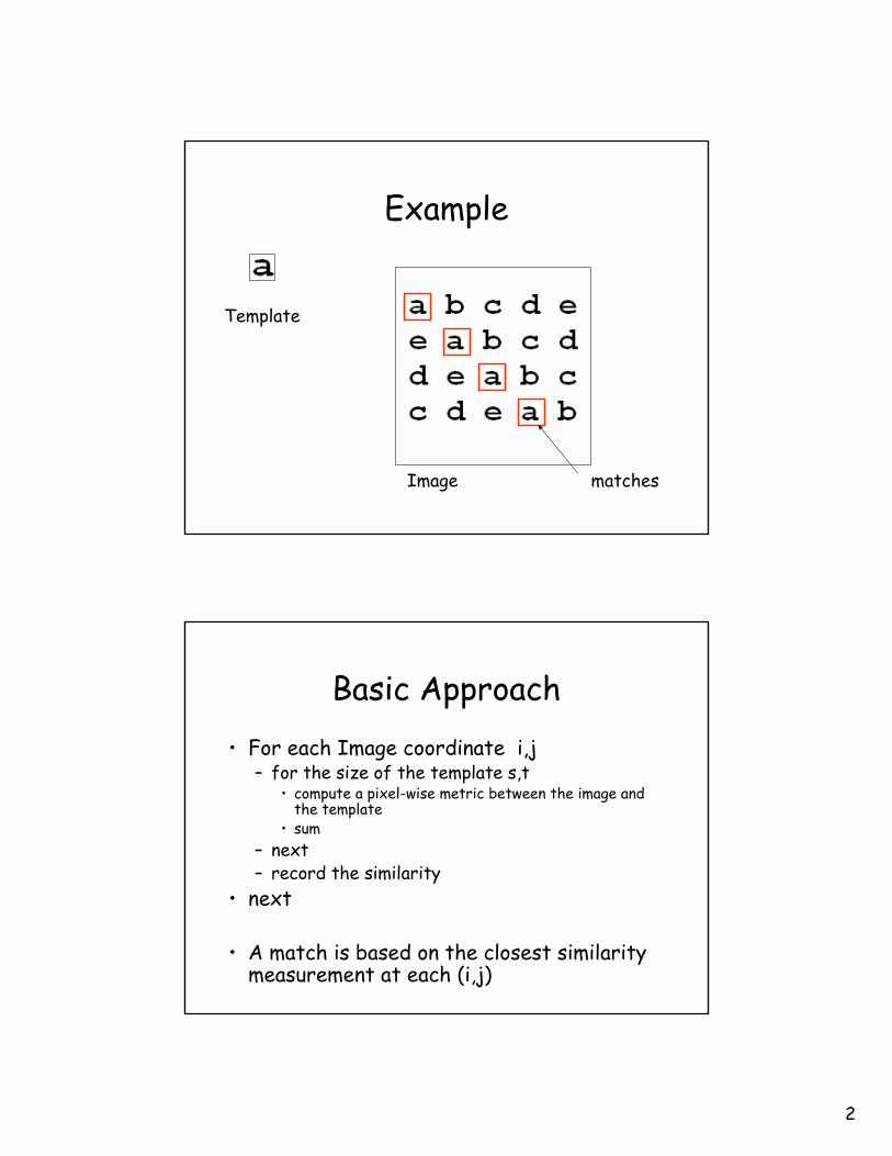
Example

Template

Image matches

Basic Approach• For each Image coordinate i,j

– for the size of the template s,t• compute a pixel-wise metric between the image and

the template• sum

– next– record the similarity

• next

• A match is based on the closest similarity measurement at each (i,j)

3

Similarity Criteria• Correlation

– The correlation response between two images fand t is defined as:

– This is often called cross-correlation

∑=yx

yxtyxfc,

),(),(

Template Matching Using Correlation

• Assume a template T with [2W, 2H]– The correlation response at each x,y is:

∑ ∑−= −=

++=W

Wk

H

Hllktlykxfyxc ),(),(),(

Pick the c(x,y) with the maximum response[It is typical to ignore the boundaries where the template won’t fit]

4

Template Matching

Matlab Example

Response Space c(x,y)(using correlation)

Problems with Correlation• If the image intensity varies with position, Correlation can

fail. – For example, the correlation between the template and an

exactly matched region can be less than correlation between the template and a bright spot.

• The range of c(x,y) is dependent on the size of the feature

• Correlation is not invariant to changes in image intensity– Such as lighting conditions

5

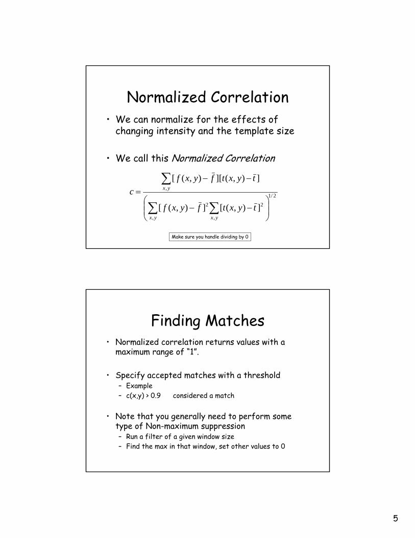
Normalized Correlation• We can normalize for the effects of

changing intensity and the template size

• We call this Normalized Correlation

2/1

,

2

,

2

,

]),([]),([

]),(][),([

⎟⎟⎠

⎞⎜⎜⎝

⎛−−

−−=

∑∑

∑

yxyx

yx

tyxtfyxf

tyxtfyxfc

Make sure you handle dividing by 0

Finding Matches • Normalized correlation returns values with a

maximum range of “1”.

• Specify accepted matches with a threshold– Example– c(x,y) > 0.9 considered a match

• Note that you generally need to perform some type of Non-maximum suppression– Run a filter of a given window size– Find the max in that window, set other values to 0

6

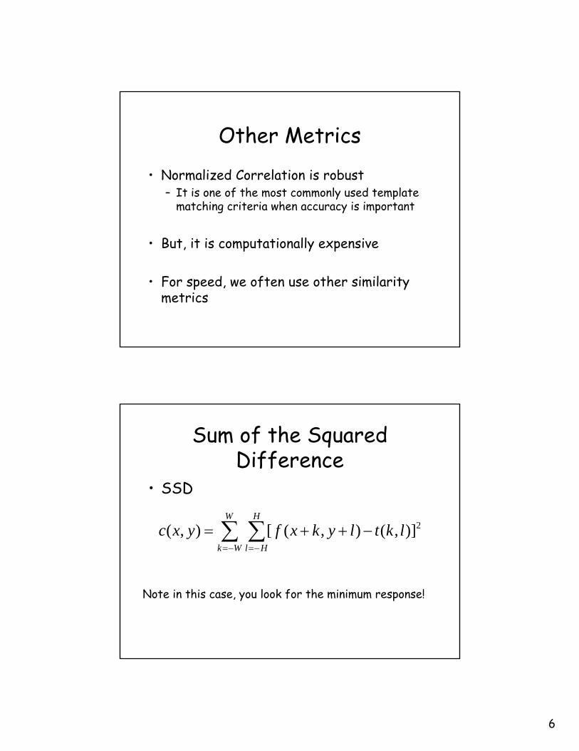
Other Metrics

• Normalized Correlation is robust– It is one of the most commonly used template

matching criteria when accuracy is important

• But, it is computationally expensive

• For speed, we often use other similarity metrics

Sum of the Squared Difference

• SSD

∑ ∑−= −=

−++=W

Wk

H

Hllktlykxfyxc 2)],(),([),(

Note in this case, you look for the minimum response!

7

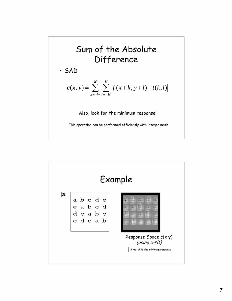
Sum of the Absolute Difference

• SAD

Also, look for the minimum response!

∑ ∑−= −=

−++=W

Wk

H

Hllktlykxfyxc ),(),(),(

This operation can be performed efficiently with integer math.

Example

Response Space c(x,y)(using SAD)

A match is the minimum response

8

Template Matching• Limitations

– Templates are not scale or rotation invariant– Slight size or orientation variations can cause problems

• Often use several templates to represent one object– Different sizes– Rotations of the same template

• Note that template matching is an computationally expensive operation– Especially if you search the entire image– Or if you use several templates– However, it can be easily “parallelized”

Template Matching

• Basic tool for area-based stereo

• Basic tool for object tracking in video

• Basic tool for simple OCR

• Basic foundation for simple object recognition

9

Object Recognition• We will discuss a simple form of object

recognition– Appearance Based Recognition

• Assume we have images of several known objects– We call this our “Training Set”

• We are given a new image– We want to “recognize” (or classify) it based on

our existing set of images

Example

http://www.cs.columbia.edu/CAVE/research/softlib/coil-20.html

Columbia University Image Library

?

10

Object Recognition• Typical Problem

• You have a training set of images of Nobjects

• You are given a new image, F– F is an image of one of these N objects

• Maybe at a slightly different view than the images in your training set

– Can you determine which object F is?

Let’s Start With Face Recognition

Database of faces [objects]

Given an “new” image,Can you tell who this is?

ftp://ftp.uk.research.att.com:pub/data/att_faces.tar.Z

11

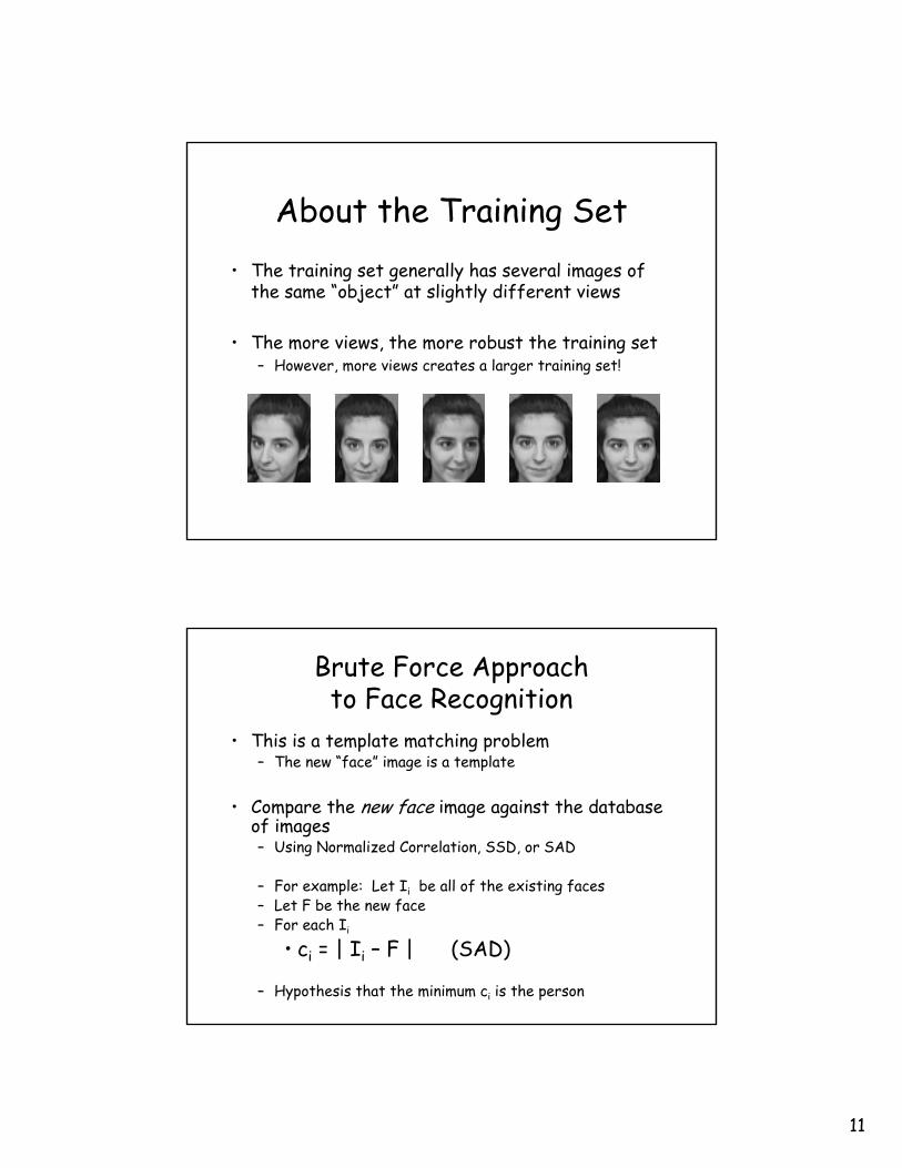
About the Training Set• The training set generally has several images of

the same “object” at slightly different views

• The more views, the more robust the training set – However, more views creates a larger training set!

Brute Force Approach to Face Recognition

• This is a template matching problem– The new “face” image is a template

• Compare the new face image against the database of images– Using Normalized Correlation, SSD, or SAD

– For example: Let Ii be all of the existing faces– Let F be the new face– For each Ii

• ci = | Ii – F | (SAD)

– Hypothesis that the minimum ci is the person

12

Example• Database of 40 people• 5 Images per person

– We randomly choose 4 faces to compose our database

– That is a set of 160 images• 1 image per person that isn’t in the

database– Find this face using the Brute force approach

• (The class example uses image of size 56x46 pixels. This is very small and only used for a demonstration. Typical image sizes would be 256x256 or higher)

Implementation• Let Ii (training images) be written as a vector• Form a matrix X from these vectors

X = I1 I2 . . . Ii . . . In-1 In

X dimensions: W*H of image * number_of_images

13

Implementation• Let F (new face) also be written as a vector

• Compute the “distance” of F to each Ii – for i = 1 to n

• s = |F - Ii|

• Closest Ii (min s) is hypothesised to be the “match”

• In class example:– X matrix is: 2576 x 160 elements– To compare F with all Ii– Brute force approach takes roughly 423,555 integer operations

using SAD

Example

50765 108711 98158 108924 99820

New Face

TrainingSet

SAD DiffImage

(Computed in Vector Form)

SAD result

14

Brute Force

• Computationally Expensive

• Requires a huge amount of memory

• Not very practical

We need a more compact representation

• We have a collection of faces– Face images are highly correlated– They share many of the same spatial

characteristics – Face,Nose, Eyes

• We should be able to describe these images using a more compact representation

15

Compact Representation• Images of faces, are not randomly distributed

• We can apply Principal Component Analysis (PCA)– PCA finds the best vectors that account for the distribution of face

images within the entire space

• Each image can be described as a linear combination of these principal components

• The powerful feature is that we can approximate this space with only a few of the principal components

• Seminal Paper: Face Recognition Using Eigenfaces– 1991, Mathew A. Turk and Alex. P. Pentland (MIT)

Eigen-Face Decomposition• Idea

– Find the mean face of the training set

– Subtract the mean from all images• Now each image encodes its variation from the mean

– Compute a covariance matrix of all the images• Imagine that this is encoding the “spread” of the variation

for each pixel (in the entire image set)

– Compute the principal components for the covariance matrix (eigen-vectors of the covariance space)

– Parameterize each face in terms of principal components

16

Eigen-Face Decomposition

X =

I1 I2 . . . Ii . . . In-1 InCompute Mean Image

X =

I1 I2 . . . Ii . . . In-1 In^ ^Compose X of

Ii = (Ii – I)

I

^ ^ ^ ^^

^

Eigen-Face Decomposition• Compute the covariance matrix

– C = X XT

• (note this is a huge matrix, size_of_image*size_of_image)

• Perform Eigen-decomposition on C– This gives us back a set of eigen vectors (ui)– These are the principal components of C

^ ^

U =

u1 u2 . . . ui . . . . . . um-1 um

17

The Eigen-Faces• These eigenvector form what Pentland called

“eigen-faces”

First 5 Eigen Faces(From our training set)

Parameterize faces as Eigen-faces

• All faces in our training set can be described as a linear combination of the eigen-faces

• The trick is, we can approximate our face using only a few eigen-vectors

Pi = UkT * (Ii – I)

Where k << Size of Image(k = 20)

Pi is onlysize k

18

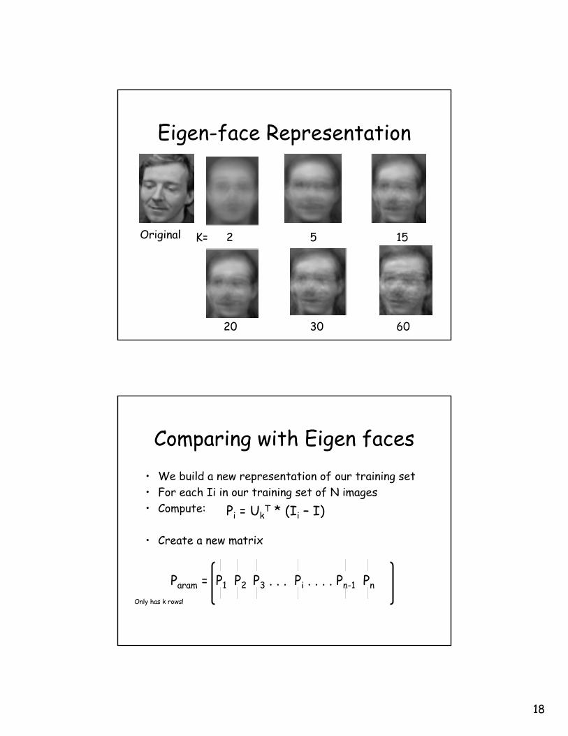
Eigen-face Representation

2 5 15

20 30 60

Original K=

Comparing with Eigen faces• We build a new representation of our training set• For each Ii in our training set of N images• Compute:

• Create a new matrix

Only has k rows!

Pi = UkT * (Ii – I)

Param = P1 P2 P3 . . . Pi . . . . Pn-1 Pn

19

Recognition using Eigen-Faces• Find a match using the parameterization

coefficients of Param

• So, given a new face F– Parameterize it in Eigenspace

– Pf = UkT * (Ii – I)

– Find the closest Pi using SAD• min | Pi – Pf |• Hypothesis image corresponding to Pi is our

match!

EigenFaces Performance• Pixel Space• In class example:

– X matrix is: 2576 x 160 elements– Brute force approach takes roughly 423,555 integer operations

using SAD

• Eigen Space• In class example

– Assume we have already calculated U and Param– Param = 20 x 160 elements– Search approach – 51,520 multiples to convert our image to eigen-space– roughly 3200 integer operations to find a match SAD !!!

20

Eigenspace Representation• Requires significant pre-processing of

space

• Greatly reduces the amount of memory needed

• Greatly reduces the “matching” speed

• Widely accepted approach

Extension to Generalized Object Recognition

• Build several eigenspaces using several training sets (one eigenspace for each set)

• Parameterize new image into these spaces– Find the closest match in all spaces– Find the closest space

21

Pose Recognition• Industrial Imaging Automation

• Take a training set of an images at difference positions– Build an eigenspace of the training set

• Given an a new image – Find its closest match in the space

• this is its “pose”

Draw backs to Eigenspaces• Computationally Expensive

• Images have to be “registered”– Same size, roughly same background

• The choice of “K” affects the accuracy of recognition

• Static representation– If you want to add a new object (person)– You have to rebuild the eigenspace

• Starts to break down when there are too many objects– You begin to get a random distribution

22

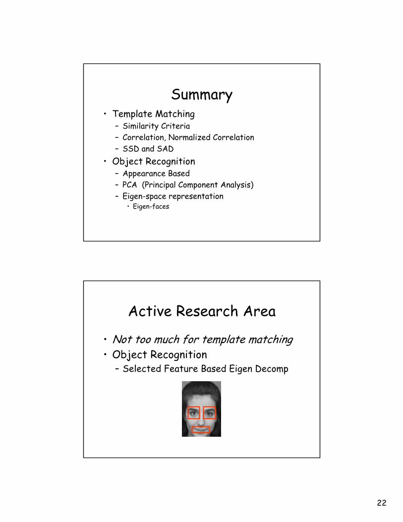
Summary• Template Matching

– Similarity Criteria– Correlation, Normalized Correlation– SSD and SAD

• Object Recognition– Appearance Based– PCA (Principal Component Analysis)– Eigen-space representation

• Eigen-faces

Active Research Area

• Not too much for template matching• Object Recognition

– Selected Feature Based Eigen Decomp

23

Active Research Area• Computing Eigenspaces

– Optimal Eigenspaces– Incremental Eigenspaces

• Face Recognition– Training set is important– Fake training images with view morphing– Compressed Domain Integration

• Eigenspace research – In math and computer vision– Very active area