50
Observa(onal study design Patrick Ryan, PhD Columbia University Janssen Research and Development

Observa(onal study design
Patrick Ryan, PhD Columbia University
Janssen Research and Development

A li@le exercise: choose your own adventure!

A pop culture mash-‐up to explain counterfactual reasoning…

Counterfactual reasoning for one person
Decision
Person Time
0 Baseline: Period to sa(sfy inclusion criteria
Follow-‐up: Period to observe
outcomes

Counterfactual reasoning for a popula(on
Cohort summary
Outcome summary

Alas, we don’t have a Delorean…
• What is our next best approxima(on?
• Instead of studying the same popula(on under both decision op(ons, let’s define a larger popula(on and randomly assign one treatment to each person, then compare outcomes between the two cohorts…

Randomized treatment assignment to approximate counterfactual outcomes
Assigned
Unobserved
Assigned
Unobserved
Assigned
Unobserved
Unobserved
Assigned
Unobserved
Assigned
Unobserved
Assigned

• Randomiza(on allows for assump(on that persons assigned to target cohort are exchangeable at baseline with persons assigned to comparator cohort
Outcome summary
Cohort summary

Alas, we can’t randomize…
• What is our next, next best approxima(on?
• Define a larger popula(on, observe the treatment choices that were made, then compare outcomes: – Between persons who made different choices (compara(ve cohort design)
OR – Within persons during (me periods with different exposure status (self-‐controlled designs)

How does Epidemiology define a compara(ve cohort study?
…it depends on what Epidemiology textbook you read… “In a retrospec(ve cohort study…the inves(gator iden(fied the cohort of individuals based on their characteris(cs in the past and then reconstructs their subsequent disease experience up to some defined point in the most recent past or up to the present (me”
-‐-‐Kelsey et al, Methods in Observa(onal Epidemiology, 1996 “In a cohort study, a group of people (a cohort) is assembled, none of whom has experienced the outcome of interest, but all of whom could experience it…On entry to the study, people in the cohort are classified according to those characteris(cs (possible risk factors) that might be related to outcome. These people are then observed over (me to see which of them experience the outcome.”
-‐-‐Fletcher, Fletcher and Wagner, Clincal Epidemiology – The Essen(als, 1996
“In the cohort study’s most representa(ve format, a defined popula(on is iden(fied. Its subjects are classified according to exposure status, and the incidence of the disease (or any other health outcome of interest) is ascertained and compared across exposure categories.”
-‐-‐Szklo and Nieto, Epidemiology: Beyond the Basics, 2007
“In the paradigma(c cohort study, the inves(gator defines two or more groups of people that are free of disease and that differ according to the extent of their exposure to a poten(al cause of disease. These groups are referred to as the study cohorts. When two groups are studies, one is usually though of as the exposed or index cohort – those individuals who have experienced the puta(ve causal event or condi(on – and the other is then thought of as the unexposed or reference cohort.”
-‐-‐Rothman, Modern Epidemiology, 2008
“Cohort studies are studies that iden(fy subsets of a defined popula(on and follow them over (me, looking for differences in their outcome. Cohort studies generally compare exposed pa(ents to unexposed pa(ents, although they can also be used to compare one exposure to another.”
-‐-‐Strom, Pharmacoepidemiology, 2005

OHDSI’s defini(on of ‘cohort’
Cohort = a set of persons who sa(sfy one or more inclusion criteria for a dura(on of (me
Objec(ve consequences based on this cohort defini(on: • One person may belong to mul(ple cohorts • One person may belong to the same cohort at mul(ple different (me
periods • One person may not belong to the same cohort mul(ple (mes during
the same period of (me • One cohort may have zero or more members • A codeset is NOT a cohort…
…logic for how to use the codeset in a criteria is required

An observa(onal compara(ve cohort design to approximate counterfactual outcomes
Observed
Unobserved
Observed
Unobserved
Observed
Unobserved
Unobserved
Observed
Unobserved
Observed
Unobserved
Observed
Observed
Unobserved
Observed
Unobserved
Unobserved
Observed
Unobserved
Observed

Outcome summary
Cohort summary
• Exchangeability assump(on may be violated if there is reason for treatment choice...and there ojen is

Propensity score introduc(on
• e(x) = Pr(Z=1|x) – Z is treatment assignment – x is a set of all covariates at the (me of treatment assignment
• Propensity score = probability of belonging to the target cohort vs. the comparator cohort, given the baseline covariates
• Propensity score can be used as a ‘balancing score’: if the two cohorts have similar propensity score distribu(on, then the distribu(on of covariates should be the similar (need to perform diagnos(c to check)
Rubin Biometrika 1983
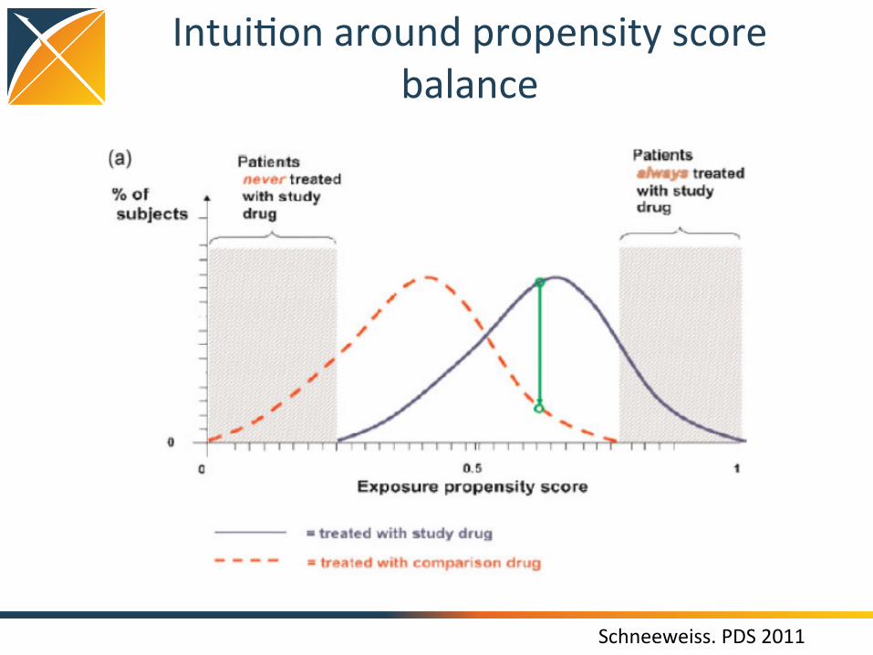
Intui(on around propensity score balance
Schneeweiss. PDS 2011

“Five reasons to use propensity score in pharmacoepidemiology”
• Theore(cal advantages – Confounding by indica(on is the primary threat to validity, PS focuses
directly on indica(ons for use and non-‐use of drug under study • Value of propensity scores for matching or trimming the popula(on
– Eliminate ‘uncomparable’ controls without assump(ons of linear rela(onship between PS and outcome
• Improved es(ma(on with few outcomes – PS allows matching on one scalar value rather than needing degrees of
freedom for all covariates • Propensity score by treatment interac(ons
– PS enables explora(on of pa(ent-‐level heterogeneity in response • Propensity score calibra(on to correct for measurement error
Glynn et al, BCPT 2006

Methods for confounding adjustment using a propensity score
Garbe et al, Eur J Clin Pharmacol 2013, h@p://www.ncbi.nlm.nih.gov/pubmed/22763756
Fully implemented in OHDSI CohortMethod R package
Not generally recommended

Matching as a strategy to adjust for baseline covariate imbalance
Observed
Unobserved
Observed
Unobserved
Observed
Unobserved
Unobserved
Observed
Unobserved
Observed
Unobserved
Observed
Observed
Unobserved
Observed
Unobserved
Unobserved
Observed
Unobserved
Observed
Cohort summary
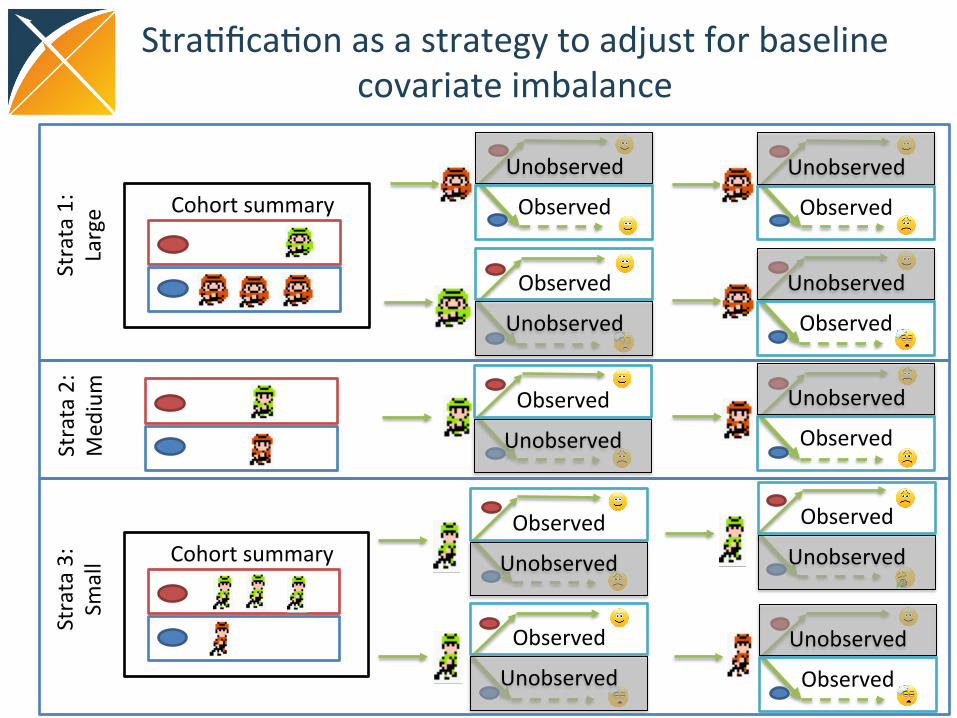
Stra(fica(on as a strategy to adjust for baseline covariate imbalance
Observed
Unobserved
Observed
Unobserved
Observed
Unobserved
Unobserved
Observed
Unobserved
Observed
Unobserved
Observed
Observed
Unobserved
Observed
Unobserved
Unobserved
Observed
Unobserved
Observed
Strata 1:
Large
Strata 3:
Small
Strata 2:
Med
ium
Cohort summary
Cohort summary

Cohort restric(on in compara(ve cohort analyses
Ini(al target cohort T
Qualifying target cohort
Analy(c target
Cohort (T’)
Ini(al comparator cohort C
Qualifying comparator cohort
Analy(c comparator cohort (C’)
Outcome cohort
Analy(c outcome cohort: O in T’, C’ during (me-‐at-‐risk

The choice of the outcome model defines your research ques(on
Logis&c regression
Poisson regression Cox propor&onal hazards
How the outcome cohort is used
Binary classifier of presence/ absence of outcome during the fixed (me-‐at-‐risk period
Count the number of occurrences of outcomes during (me-‐at-‐risk
Compute (me-‐to-‐event from (me-‐at-‐risk start un(l earliest of first occurrence of outcome or (me-‐at-‐risk end, and track the censoring event (outcome or no outcome)
‘Risk’ metric Odds ra(o Rate ra(o Hazard ra(o
Key model assump(ons
Constant probability in fixed window
Outcomes follow Poisson distribu(on with constant risk
Propor(onality – constant rela(ve hazard

When designing or reviewing a study, ask yourself:
Input parameter Design choice
Target cohort (T)
Comparator cohort (C)
Outcome cohort (O)
Time-‐at-‐risk
Model specifica(on

Exercise 1
• Define your own problem

Break

Exercise 2
• Apply the framework to a published paper

Observa(onal study design Part #2
Patrick Ryan, PhD Columbia University
Janssen Research and Development

Design an observa(onal study like you would a randomized trial
Protocol components to emulate: • Eligibility criteria • Treatment strategies • Assignment procedures • Follow-‐up period • Outcome • Causal contrasts of interest • Analysis plan

• Bias = expected value of the error distribu(on
BIAS[ 𝜃 ] = 𝐸[ 𝜃 −𝜃] = 𝐸[𝜃 ]−𝜃
where 𝜃 = true value, 𝜃 = es(mate of 𝜃
• Mean squared error = metric to evaluate the quality of an es(mator, accoun(ng for both random and systema(c error
MSE[𝜃 ] = 𝐸[ ( 𝜃 −𝜃)↑2 ] = (BIAS[𝜃 ])↑2 +
𝑉𝑎𝑟[ 𝜃 ] As studies increase in sample size, random error converges to 0 but systema(c error s(ll persists!
Types of systema(c error
• Confounding • Misclassifica(on (Measurement error) • Selec(on bias (generalizability)

Confounding
A Y Effect of interest RR=???
A=exposure Y=outcome
C
C = observed and modeled confounder
U
U = unobserved or mismodeled confounder
Challenge: Producing an ‘unconfounded’ es(mate relies on (empirically untestable) assump(on that 1) all confounders were observable, and properly modeled in the design or analysis, and 2) no unobserved factors are associated with both exposure and outcome

How do you assess confounding?
• PS distribu(on • Covariate balance

Misclassifica(on (measurement error)
A Y Effect of interest RR=???
C
U
Challenge: All observa(ons are imperfect proxies for true pa(ent status. Misclassifica(on error can exist for all exposures, outcomes and covariates, but is generally unknown or not properly es(mated (via sensi(vity and specificity), and is rarely formally integrated into effect es(ma(on.
A* Y*
C*
A*=proxy for exposure Y*=proxy for outcome
A=exposure Y=outcome C = observed and modeled confounder U = unobserved or mismodeled confounder
C* = proxy for observed confounder
Es(mate we observe

How do you assess measurement error?
• Covariate summary for exposures • Opera(ng characteris(cs for outcome phenotype – Sensi(vity – Specificity – Posi(ve predic(ve value

Selec(on bias and generalizability
A Y Effect of interest RR=???
C
U
Challenge: A database is a non-‐random sample of an underlying popula(on. A cohort is a non-‐random sample of the database. Study design and analysis decisions may further restrict the cohort composi(on. Selec(on bias is rarely evaluated and ojen empirically untestable.
A#
A#=non-‐random sample of exposure A=exposure Y=outcome C = observed and modeled confounder U = unobserved or mismodeled confounder
Es(mate we observe

How do you assess selec(on bias?
• A@ri(on table • Covariate summary (compare before to ajer)

What can we do to address these challenges?
• Think really hard during study design and hope we get it right
• Equivocate in our summary of findings with a paragraph in the Discussion that reads: – “This study has several limita(ons. First, since this study relied on claims data, we had no data on <unobserved confounders>. Second, while we adjusted for <observed confounders>, residual confounding cannot be ruled out. Third, there is a poten(al for outcome misclassifica(on… Fourth, there is a poten(al for duplicate person-‐years between <databases>. Lastly, as the mean follow-‐up was <short>, long-‐term effects may need to be further examined.” (Kim et al., Arthri(s & Rheumatology, 2017)
• •

What can we do to address these challenges?
• Think really hard during study design and hope we get it right
• Equivocate in our summary of findings with a paragraph in the Discussion that reads: – “This study has several limita(ons. First, since this study relied on claims data, we had no data on <unobserved confounders>. Second, while we adjusted for <observed confounders>, residual confounding cannot be ruled out. Third, there is a poten(al for outcome misclassifica(on… Fourth, there is a poten(al for duplicate person-‐years between <databases>. Lastly, as the mean follow-‐up was <short>, long-‐term effects may need to be further examined.” (Kim et al., Arthri(s & Rheumatology, 2017)
• Perform diagnos(c analyses that a@empt to detect if residual error may s(ll be present
• Quan(fy magnitude of residual error and calibrate sta(s(cs

Examples of nega(ve controls
Infec(ous mononucleosis
Mul(ple sclerosis ? Rubella
Measles
?
?
38

Example of a nega(ve control
Infec(ous mononucleosis
Mul(ple sclerosis 1.31 * Rubella
Measles
2.22 *
1.42 *
* P < .05
Odds ra(o:
39

Example of a nega(ve control
Infec(ous mononucleosis
Mul(ple sclerosis
1.31 * Rubella
Measles
2.22 *
1.42 *
A broken arm
1.23 * Concussion
Tonsillectomy
1.10
1.25 *
Nega(ve controls:
* P < .05
Odds ra(o:
40

Key points: • 2 types of nega(ve controls:
• Exposure controls • Outcome controls
• “In principle, the measured confounders L of the A-‐Y rela(onship need not be causes of N as well, because a properly specified model that accounted for the confounding by L of A-‐Y would not be misled if such confounding were absent for A-‐N.”
• “In prac(ce, the ideal nega(ve control outcome should be one with incoming arrows as similar as possible to those of Y, including arrows from L”
• “In observa(onal se{ngs, the comparability between exposure A and nega(ve control exposure B will be only approximate”
• “Subject ma@er knowledge is required for the choice of nega(ve controls”

Key points: • “A falsifica(on hypothesis is a claim, dis(nct from the one being tested,
that researchers believe is highly unlikely to be causally related to the interven(on in ques(on.”
• “Falsifica(on analysis can be opera(onalized by asking inves(gators to specify implausible hypotheses up front and then tes(ng those claims using sta(s(cal methods similar to those used in the primary analysis.”
• “Although no published recommenda(ons exist, standardized falsifica(on analyses with 3 or 4 prespecified or highly prevalent disease outcomes may help strengthen the validity of observa(onal studies”

Key points: • “The extent to which an analysis may reveal unobserved confounding bias
relies on the non-‐empirically verifiable assump(on that the nega(ve control outcome is carefully chosen so that it is solely influenced by observed and unobserved confounders of the exposure-‐outcome rela(onship in view”
• “We propose to use a nega(ve control outcome not only to detect, but also to correct for unmeasured confounding bias”
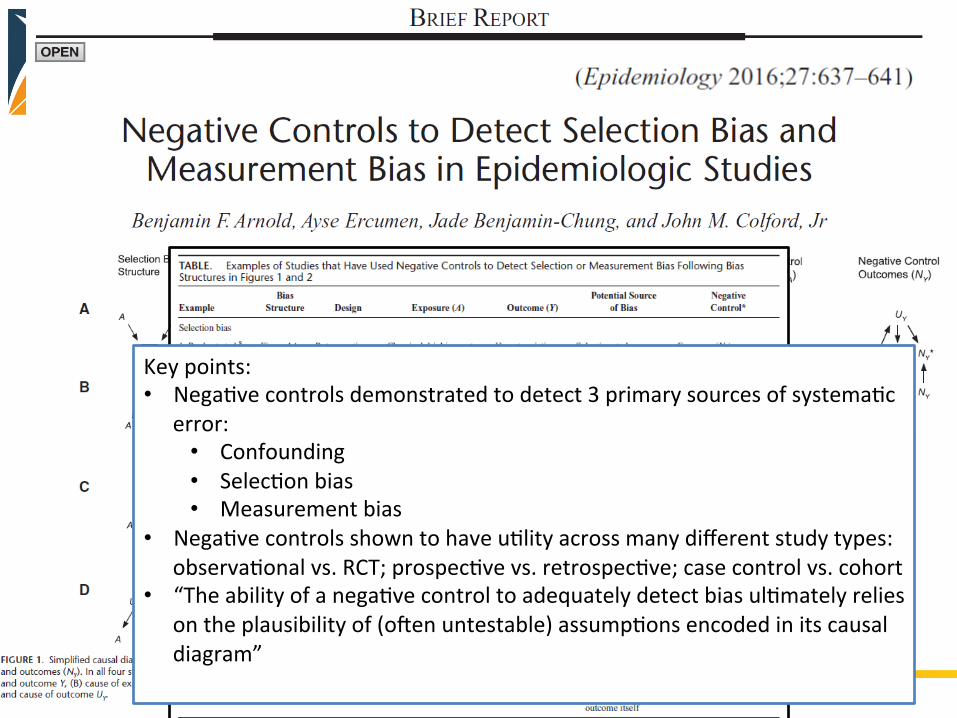
Key points: • Nega(ve controls demonstrated to detect 3 primary sources of systema(c
error: • Confounding • Selec(on bias • Measurement bias
• Nega(ve controls shown to have u(lity across many different study types: observa(onal vs. RCT; prospec(ve vs. retrospec(ve; case control vs. cohort
• “The ability of a nega(ve control to adequately detect bias ul(mately relies on the plausibility of (ojen untestable) assump(ons encoded in its causal diagram”


Exercise 3
• Evaluate Graham, what did they do to mi(gate the threat of systema(c error? How do you know they were successful?


