Abstract Knowledge of upper ocean currents is neededfor trajectory forecasts and is essential for search andrescue operations and oil spill mitigation. This paperaddresses effects of surface waves on ocean currentsand drifter trajectories using in situ observations.The data set includes colocated measurements ofdirectional wave spectra from a wave rider buoy, oceancurrents measured by acoustic Doppler currentprofilers (ADCPs), as well as data from two types oftracking buoys that sample the currents at two differentdepths. The ADCP measures the Eulerian current atone point, as modelled by an ocean general circulationmodel, while the tracking buoys are advected by theLagrangian current that includes the wave-inducedStokes drift. Based on our observations, we assess theimportance of two different wave effects: (a) forcing ofthe ocean current by wave-induced surface fluxes andthe Coriolis–Stokes force, and (b) advection of surfacedrifters by wave motion, that is the Stokes drift. Recent
Responsible Editor: Arthur Allen
This article is part of the Topical Collection on Advances inSearch and Rescue at Sea
J. Röhrs (B) · K. H. Christensen · L. R. Hole · M. DrivdalNorwegian Meteorological Institute,Allegaten 70, 5007 Bergen, Norwaye-mail: [email protected]
G. BroströmDepartment of Earth Science,University of Gothenburg,Gothenburg, Sweden
S. SundbyInstitute of Marine Research,Nordnesgaten 50, 5005 Bergen, Norway
theoretical developments provide a framework forincluding these wave effects in ocean model systems.The order of magnitude of the Stokes drift is the sameas the Eulerian current judging from the available data.The wave-induced momentum and turbulent kineticenergy fluxes are estimated and shown to be significant.Similarly, the wave-induced Coriolis–Stokes force issignificant over time scales related to the inertialperiod. Surface drifter trajectories were analysed andcould be reproduced using the observations of currents,waves and wind. Waves were found to have a significantcontribution to the trajectories, and we conclude thatadding wave effects in ocean model systems is likelyto increase predictability of surface drifter trajectories.The relative importance of the Stokes drift was twiceas large as the direct wind drag for the used surfacedrifter.
The drift velocity of a floating object depends on howit responds to the geophysical forcing represented bythe wind, the surface waves, and the ocean currents(Daniel et al. 2002; Breivik and Allen 2008). Oper-ational forecasting centres that provide services forsearch and rescue need to have access to these physicalparameters. Usually, there are three separate numericalmodel systems for the atmosphere, the surface wavesand the ocean circulation, respectively, with variousdegrees of coupling between the systems.
1520 Ocean Dynamics (2012) 62:1519–1533
The response of a floating object to wind can bemodelled by assessing the leeway, which is the pathrelative to the wind (Breivik et al. 2011). The advectionby the ocean currents includes parts which are dueto the mean drift inherent in surface waves (Stokes1847) and also the mean currents forced by the waves(Longuet-Higgins 1953). Several approaches exist toaccount for these wave effects, but, in many cases,they are fully parameterized using only wind speedand direction, hence removing the need for a separatewave model. Such parametrisations implicitly assumethat the waves are always correlated with the localwind, something which is often not the case. In thispaper, we will focus on the benefit of having a dedicatedwave forecasting system in the context of trajectoryforecasts.
Taking wave effects into account for ocean and tra-jectory models has been an effort during the recentyears. First approaches parametrise turbulent fluxesfrom waves to the current (Craig and Banner 1994)using the wind speed. Carniel et al. (2009) use thisapproach to model surface trajectories. Other studies(Broström et al. 2008; Jenkins 1989) discuss the purposeof numerical wave models to calculate momentum andenergy fluxes between waves and the current. An ap-plication of the approach by Jenkins (1989) to surfacedrifters was made by Perrie et al. (2003) and Tang et al.(2007). Observations that relate waves effects to driftertrajectories are rare, but, for example, Ardhuin et al.(2009) estimates the current as well as the wave motionusing HF radar data.
This study presents in situ measurement of waves,currents and drifter trajectories. We focus on openocean conditions, hence we do not discuss near-shoreor shallow water dynamics. We discuss the benefits ofhaving coupled model systems, in particular coupledwave and ocean models. The most common approachtoday is to have a split, one-way coupling for the air–sea momentum and energy fluxes: the wind forces boththe waves and the ocean circulation, and there is nocoupling between the wave and the mean currents.
We use data collected during a research cruisein April 2011. The data set contains observationsfrom drifting buoys, acoustic Doppler current profilers(ADCPs), and directional wave buoy, as well as ship-based measurements of wind speed and direction. Incontrast to previous drifter studies (Perrie et al. 2003;Carniel et al. 2009), which only consider one type ofdrifting buoy, we deployed two types that sample thecurrents at different depths. Furthermore, the directwave measurements enable us to make good estimatesof the Stokes drift, and the wave dependent fluxes andbody forces.
The outline of the paper is as follows: In Section 2,we give a theoretical introduction on drifter dy-namics and wave–current interactions. The measure-ment location and the instrumentation is described inSection 3, and in Section 4, we summarise the obser-vations. Section 5 is devoted to the evaluation of thevarious wave effects and analysis of the drifter data.Finally, Section 6 contains some concluding remarks.
2 Theoretical aspects
2.1 Dynamics of a drifting object
The equation of motion for a drifting object with massm and drifter position x can be written (Breivik andAllen 2008; Daniel et al. 2002):
md2xdt2 = FC + Fa + Fo + Fw, (1)
where FC is the Coriolis force, Fa the wind drag, and Fo
the water drag. The force Fw is the force due to scatter-ing of waves. Our drifter buoys are small compared totypical wavelengths, and the latter force will be ignoredhere. Wind and water drag can be expressed by therelative velocity of the drifter to the respective medium(O’Donnell et al. 1997). For instance, the water sidedrag force for small objects is
Fo = 12ρw AwCw
∣∣∣∣uL − dx
dt
∣∣∣∣
(
uL − dxdt
)
. (2)
Here, ρw is the water density, Aw the effective area thatis exposed to the water, Cw a drag coefficient and uL theLagrangian (particle following) current in the water.
2.2 Modelling mean currents and waves
Equation 2 requires the knowledge of ocean currents.Most numerical ocean circulation models use anEulerian description of the motion and the currentsfrom such models will be denoted by uE. A significantpart of the upper ocean drift velocities is due to theStokes drift, which is the intrinsic forward motion as-sociated with surface gravity waves (Stokes 1847). Ina wave, the fluid particles describe near closed orbits,but they travel slightly further forward beneath thewave crest compared to the backward motion beneaththe trough. This difference results in a net forwardtransport in the wave propagation direction. This thedirect effect of waves on drifting objects.
Ocean Dynamics (2012) 62:1519–1533 1521
The Stokes drift is a Lagrangian quantity (i.e., par-ticle following), which means that it cannot be repre-sented in conventional ocean circulation models thatuse an Eulerian description (e.g. Broström et al. 2008).
The Stokes drift will here be denoted uS. It is definedas the difference between the Lagrangian and Eulerianvelocities and it is customary to write (e.g. Craik 1982)
uL = uE + uS. (3)
From numerical wave prediction models, we can obtainreliable forecasts of the directional wave spectra, whichgive complete information about the Stokes drift uS.These models are based on a statistical description ofthe sea surface height, in which the waves are repre-sented by a two-dimensional variance spectrum E. Wedefine the wave frequency ω, the wave number k andpropagation direction θ . Introducing the unit vectorik = k/|k|, the phase and group velocities of the wavesare cp = (ω/|k|)ik and cg = ∂ω/∂k, respectively.
The wave models solve the action balance equation,which evolves the spectrum forwards in time accordingto the source terms Si (Komen et al. 1994). A simplifiedversion of this equation, suitable for deep-water wavesand assuming negligible current refraction, is
(∂
∂t+ cg · ∇
)
E = Sin + Snl + Sdis, (4)
where Sin represents wave growth due to the action ofthe wind, Sdis wave dissipation due to breaking/whitecapping, Snl nonlinear wave–wave interactions that dis-tribute energy between the different wave components.The nonlinear interaction term only redistributes mo-mentum and energy between the different wave com-ponents, which means that the integral of Snl over allwave components is zero.
Correct to the second order in the wave steepness,the Stokes drift can be written as (e.g. Jenkins 1989)
uS = 2∫ 2π
0
∫ ∞
0Eωk exp(2|k|z)dωdθ, (5)
In Eq. 5, we have used the fact that deep-water wavesdecay exponentially with depth. The magnitude andvertical shear of the Stokes drift crucially depends onthe wave conditions: young wind sea with predomi-nantly short waves has a Stokes drift with high surfacespeeds and strong vertical shear, while long period swellis associated with a Stokes drift that is much moreuniformly distributed with depth.
2.3 Wave-induced forcing of the Eulerianmean currents
An important point to make here is that the Eulerianmean current uE will not be unaffected by the waves.On the contrary, it will be influenced by wave de-pendent air–sea fluxes of momentum and energy andby wave-induced body forces. We will briefly describesome of the more well-known wave effects and pointout some physical inconsistencies that appear whenthese effects are ignored.
A significant part of the total atmospheric momen-tum and energy fluxes goes into the wave field. Whenthe waves dissipate, e.g., through wave breaking/whitecapping, there is a flux of momentum and turbulentkinetic energy from the waves to the ocean. The mo-mentum flux is manifested as a surface (or near surface)stress that accelerates the mean flow (Longuet-Higgins1953; Weber 1983; Jenkins 1989; Weber et al. 2006),while the energy flux cause enhanced near surface tur-bulent mixing (Craig and Banner 1994). In the absenceof any wave dissipation, the momentum and energycontained in the wave field is simply advected by thewaves at the wave group velocity. The wave field shouldtherefore be regarded as a reservoir of mean momen-tum and energy.
In the simplest coupled system, the wave model actsas a filter between the atmosphere and the ocean, ad-justing the air–sea fluxes according to the wave energybudgets. The wave-induced momentum and energyfluxes can be calculated from the source terms in Eq. 1,for example, the momentum flux τo into the ocean is(Saetra et al. 2007)
τo = τa − ρwg∫ 2π
0
∫ ∞
0
kω
(Sin + Sdis)dωdθ, (6)
where τa is the total atmospheric momentum flux.The total atmospheric flux is, in general, sea state-dependent (Janssen 1989), but is often calculated fromthe wind speed and direction using bulk flux formulae(e.g. Smith 1988). From Eqs. 4 and 6, we see thatwhenever the source terms are unbalanced and thewave field is changing, there is a corresponding changein the effective momentum flux to the ocean.
As an example of the importance of Eq. 6, considera situation with growing waves. The momentum inthe waves, and hence the Stokes drift velocity, thenincreases. The integral in Eq. 6 will be positive andthe effective momentum flux τ o to the mean Euleriancurrents will be smaller than τ a. If we force our oceanmodel with the total flux τ a and neglect the waveeffects, the Eulerian current will be overestimated. If
1522 Ocean Dynamics (2012) 62:1519–1533
we then add the Stokes drift and the Eulerian meancurrents to obtain the Lagrangian current, we see thatthe same momentum increase appears twice: first as anincrease in the Stokes drift and second as an increasein the Eulerian mean currents. Thus, adding the Stokesdrift to ocean model currents without accounting forthe wave-induced fluxes violates the fundamental phys-ical principle of momentum conservation and is detri-mental for the current predictions.
Similarly, the energy flux from the atmosphere to thewaves can be expressed in terms of the input sourcefunction
�aw = ρwg∫ 2π
0
∫ ∞
0Sindωdθ, (7)
while the energy flux from the waves to the ocean canbe expressed as
�wo = ρwg∫ 2π
0
∫ ∞
0Sdisdωdθ. (8)
This flux is a result of wave breaking/white-cappingand wave–turbulence interactions and increases theturbulent kinetic energy (TKE) in the upper layer ofthe ocean (e.g. Rascle and Ardhuin 2009). Definingthe total atmospheric energy flux �a, we can write ananalogue to Eq. 6 for the flux �o into the ocean as
�o = �a − ρwg∫ 2π
0
∫ ∞
0(Sin + Sdis)dωdθ. (9)
The direct flux of TKE from the air flow to the oceanis usually considered to be small compared to the otherterms (Phillips 1977).
Wave–mean current interactions have been studiedfor a long time in the context of weakly nonlinear the-ory. These interactions can be broadly divided in twocategories: (a) large scale dissipative or non-dissipativewave, mean-flow interactions and Coriolis forces and(b) small scale dispersion and mixing due to nonlinearinstability mechanisms. Large scale here means spatialand temporal scales much larger than the wavelengthand period of the waves. Processes in the first categorywill typically be modelled as wave dependent forcingterms in the ocean circulation models. As an exam-ple, one can consider the radiation stresses induced bybreaking swell in the near-shore (Longuet-Higgins andStewart 1964; Weber et al. 2009). In deep water, thedominating contributions are the wave-dependent air–sea fluxes and the so-called Coriolis–Stokes force (fCS)(Polton et al. 2005; Weber et al. 2008). This latter force
is simply the contribution to the Coriolis force from theStokes drift:
fCS = −ρw f k × uS, (10)
where f is the Coriolis parameter and k is the unitvector pointing upwards.
Processes that belong to the second category in-clude wave–turbulence-mean flow interactions andsmall scale circulations such as Langmuir turbulence(Craik and Leibovich 1976; Grant and Belcher 2009).These processes will not be addressed in this paper.
3 Field campaign
The field campaign took place in northern Norway onApril 8–13 in 2011. The Institute of Marine Researchin Bergen, Norway, has yearly research cruises in theVestfjorden area during the spawning season of theAtlantic Cod, which raises a particular interest inoceanic conditions in this area.
3.1 Measurement site
Vestfjorden in northern Norway is a wide triangularformed ocean bay bounded along the southeast bya highly mountainous roughed coast intercepted bybranched deep fjords (Fig. 1). On the other side, in thenorthwest, it is bounded by the Lofoten archipelago,another roughed mountain chain intercepted by shal-low tidal sounds towards the outer part of the coast.The length of the ocean bay from the head to themouth is about 180 km, and the width at the mouth is70 km. The bottom topography is though similar to areal fjord with a deep basin extending down to 700-mdepth towards the head and a sill depth of 220 m nearthe mouth.
The main part of the Norwegian Coastal Current ispassing by the mouth of Vestfjorden. A smaller fractionis turning into Vestfjorden flowing in along the south-east side and out in a narrower band (Roed 1980) alongthe Lofoten Archipelago. The surrounding mountaintopography exerts strong influence on the atmosphericcirculation above the fjord (Sundby 1982; Jones et al.1997).
While the flow along the mountain borders on eachside of Vestfjorden is rather unidirectional, the centralpart of the system is dominated by eddies of varioussizes (Michelson-Jacob and Sundby 2001). The largesteddies, about 50 km in diameter, occur in the outer
Ocean Dynamics (2012) 62:1519–1533 1523
Fig. 1 Drifter trajectories in the Vestfjorden bay at the coastof Nordland, Norway. The inlet map shows the location ofVestfjorden in Norway. Bathymetry contours are shown with20-m intervals and blue shading. Mooring stations during theBioWave Cruise 2011 are shown by coloured markers, the threestations are arranged as a triangle with about a kilometre dis-tance to another with following instruments: blue dot, ADCPmooring; green dot, wave rider mooring. Trajectories of SLDMBand iSphere drifters until April 12 at 0000 hours are shown in
colours. Deployment times for each drifter are shown in Table 1,initial positions are marked by red stars. Black diamonds in-dicate full 6-h steps (0000, 0600, 1200 and 1800 hours UTC).The SLDMBs (solid lines) perform a southwesterly motion withclockwise turning loops. The iSpheres (dotted lines) that werelaunched during the first deployment start with a southwesterlymotion before they turn northwards, while the iSpheres that werelaunched during the second deployment start with a northerlymotion followed by a anticyclonic loop
parts of the bay near the sill and are generally an-ticyclonic. The smaller eddies towards the head areabout 20 km in diameter and less. These are generallycyclonic. The observed eddies are generally extendingthroughout the mixed layer depth which may vary dur-ing spring between 50 and 150 m.
Three different moorings were deployed during thecruise. They were positioned approximately 2 km apartforming a triangle. The first mooring contained twoADCPs, the second was the wave rider buoy and thethird an experimental buoy for measuring oceanic tur-bulence. The locations of these moorings are shown inFig. 1. The research vessel made short excursions fromthe moorings but was mostly on station in the middle ofthe triangle.
3.2 Wind measurements
This experiment was carried out with the research ves-sel “Johan Hjort” of the Institute of Marine Research.A wind vane from the Norwegian Meteorological Insti-tute is installed on this vessel at approximately 19.5 mhigh above sea level. On April 9 at 1800 hours andApril 11 at 1600 hours, the vessel stayed within 5 kmof the measurement site, providing wind speed anddirection for the presented analysis.
3.3 Directional wave rider buoy
Wave measurements were taken with a DatawellDWR-MkII directional wave rider buoy (Datawell
1524 Ocean Dynamics (2012) 62:1519–1533
2007). Vertical and horizontal accelerations along withorientation were measured to yield heave and lateraldisplacements. The wave buoy measures waves withperiods ranging from 1.6 to 30 s and heave with a reso-lution of 0.01 m within a range of −20 to 20 m at a sam-pling frequency of 1.28 Hz. The output from the wavebuoy are the power spectral density E( fn) and the meanwave direction φn for each discrete wave frequencyfn. Such spectra are produced every half hour. Thewave rider was deployed during the period April 9 at1122 hours to April 12 at 1722 hours at the positionshown in Fig. 1 (green marker).
3.4 Ocean currents
Oceanic current velocities during the experiment inVestfjorden were observed using ADCPs. While theseinstruments measure vertical profiles of the Eulerianvelocities, the drifters described in Section 3.5 allow toassess Lagrangian velocities.
Two ADCPs were used, one at 12-m depth and oneat the bottom, both looking upwards. The ocean depthat this place is 121 m. The ADCP at the surface is a1-MHz Nortek Aquadopp ADCP. It recorded 2-minaverages of velocities in 25-cm-large vertical bins. Dataof the two uppermost wet bins and four bins in 7–8-mdepth had to be disregarded due to surface backscat-tering and ringing effects. The bottom ADCP at 118-mdepth is a 190-kHz Nortek Aquadopp ADCP. Itrecords 2-min averages in 2-m bins.
The high signal frequency of the upper ADCP allowsto sample high vertical resolution profiles of the uppermixed layer, giving a particular opportunity to studysurface processes. We used the bottom ADCP with lowresolution and high measurement range to cover thecolumn underneath the upper ADCP.
ADCP data bins were mapped to depth levels foreach time step. The data bin intersecting the sea surfaceis recognised by a maximum of backscatter amplitude.Valid data from ADCP 1 is available between thedepths of 0.5 and 10 m. Valid data of ADCP 2 reachesfrom the depths of 15–115 m.
All ADCP data were low-pass-filtered with a Godin-type time filter over 15 data points, which removessignals with periods of less than 30 min (Emery and
Thomson 1997). We applied an additional vertical filterto all upper ADCP profiles because the low size of thebins (25 cm) caused noisy velocity estimates. Much ofthat noise was reduced by a weighted average filter overthree bins, where the centre bin had twice the weight ofthe adjacent bins.
3.5 Drifting buoys
Two types of surface drifters were deployed duringthe BioWave Cruise. Six CODE-type (self-locating da-tum marker buoy (SLDMB) from MetOcean, Canada)drifters were used. These drifters follow the current atapproximately 1-m depth and are not directly affectedby wind (Davis 1985a). They consist of a cross-shapedsail extending from 0.3- to 1.2-m depth underneath thesurface with small floats at the surface.
We also deployed six surface drifters (iSpheres fromMetOcean). These are spheric floats with a diameterof 35 cm, being half-submerged in water and thereforeexposed to the wind. They have an aerodynamicallysmooth shape, and previous studies indicate that thistype of drifter shows similar behaviour as crude oil(Aamo and Jensen 1997). Their main use is for oil spilltracking (Belore et al. 2011).
Both drifter types transmit their positions over theIridium satellite network. SLDMB drifter positions arereported every 10 min, while iSphere positions arereported every 30 min. The SLDMBs drifters stayed inthe interior parts of Vestfjorden for more than a week,while all the iSpheres stranded after a few days duringa strong wind event. Deployment times are listed inTable 1.
4 Meteorological and oceanographic conditions
4.1 Wind and waves
The weather situation during the period of interestwas dominated by passing low pressure systems; onApril 9 at 0000 hours, there was a low pressure sys-tem located between Norway and Spitsbergen, whichgave westerly winds over Lofoten. This low pressuremoved northwards, and a new low pressure system
Fig. 2 Measurements at mooring station in Vestfjorden duringApril 9 at 1800 hours–April 12 at 0000 hours. a Wind speed andsignificant wave height. b Wind direction and direction of theStokes drift at the surface. c Mean zero up-crossing wave period.
d Eulerian current at 0.5-m depth (dashed lines) and Stokes driftat the surface (solid lines). Easterly and northerly componentsare shown, respectively
moved in from Iceland, moving northwards towards theGreenland coast. The wind direction over Lofotenchanged to south–southwest with 8 m/s by 0600 hourson April 10 (Fig. 2a, b). As the low pressure systemdeepened and moved further northwards, the wind
picked up to a maximum of 15 m/s while the directionremained rather constant.
Waves were governed by the prevailing southwest-erly winds, and the significant wave height was up to1.5 m at the experiment site (Fig. 2a, b). Figure 2c
1526 Ocean Dynamics (2012) 62:1519–1533
shows long wave periods before April 10 at 0600 hours,hence some swell was entering Vestfjorden. As thewind picked up from the south, the Lofoten peninsulano longer acted to shelter the waves and the significantwave height picked up to become 2.2 m at about1400 hours on April 10 at the experiment site. After thisevent, the significant wave height declined slowly as thewind ceased. The wave period was constant in the decayphase, and it is likely that some swell is present in thedecay period.
4.2 Ocean circulation
The general ocean circulation during the cruise is inagreement with the historically observed circulationpattern. Vertical averaged ADCP data show a domi-nant current towards southwest. This is consistent withthe cyclonic eddy reported by Michelson-Jacob andSundby (2001), being located in its northwestern seg-ment. This eddy is typically dominating the circulationin Vestfjorden.
A harmonic analysis of ADCP currents was per-formed using the software of Pawlowicz et al. (2002).Tidal motion, whose major constituent is the lunarcomponent M2, is limited to the zonal velocities of thebarotropic current. Spectral analysis of upper oceancurrents above 10-m depth show peaks at 13.1 ± 1.0 h.This peak is close to the tidal period TM2 = 12.4 h aswell as to the inertial period Tint = 12.9 h. A transientsignal with such a period in the ADCP data shows anupward propagating internal wave phase. This impliesdownward propagating energy, which means that thewave is generated at the surface (Alford and Gregg2001), most likely during the strong winds on April 10(Fig. 2a). This wind event created an inertial oscillation,which is also evident from the drifter data where itappears as anticyclonic loops in the trajectories (Fig. 1).
Measured surface currents and Stokes drift duringthe experiment are shown in Fig. 2d. Components ofEulerian current at 0.5-m depth are shown; this is theuppermost layer that could be observed by the ADCP.The Stokes drift at the surface (0-m depth) is calculatedfrom the measured directional wave spectra accordingto Eq. 5. Throughout the experiment, the magnitudeof the Stokes drift is on average 20 % of the Euleriancurrent. During the wind event on the 10th of April, be-tween 1200 hours and 1800 hours, the Stokes drift evenreaches the same magnitude as the Eulerian current.Notably, the Stokes drift has a rather unidirectionalbehaviour, while the Eulerian current exhibits muchmore high-frequency variations. As for example, the
inertial oscillation described above appears as strongperturbation on April 10 and April 11 in both compo-nents of the Eulerian current.
5 Analysis of drifter and wave buoy data
5.1 Drifter deployments
Two types of drifters were deployed to study differ-ences in their behaviour and to compare their driftwith observed geophysical fields. Drifters were released5 km close to the mooring triangle. The iSpheres stayedwithin 14-km distance to the moorings; their trajecto-ries are related to ADCP currents and the wave field inSection 5.4.
Unintentionally, the SLDMB drifters moved awayfrom the moorings. Located at 1-m depth, they fol-lowed the general current pattern southwestwards, asdescribed in Section 3.1. Contrary, the iSpheres at 0-mdepths moved somewhat with wind and waves towardsnorth as expected (Fig. 1).
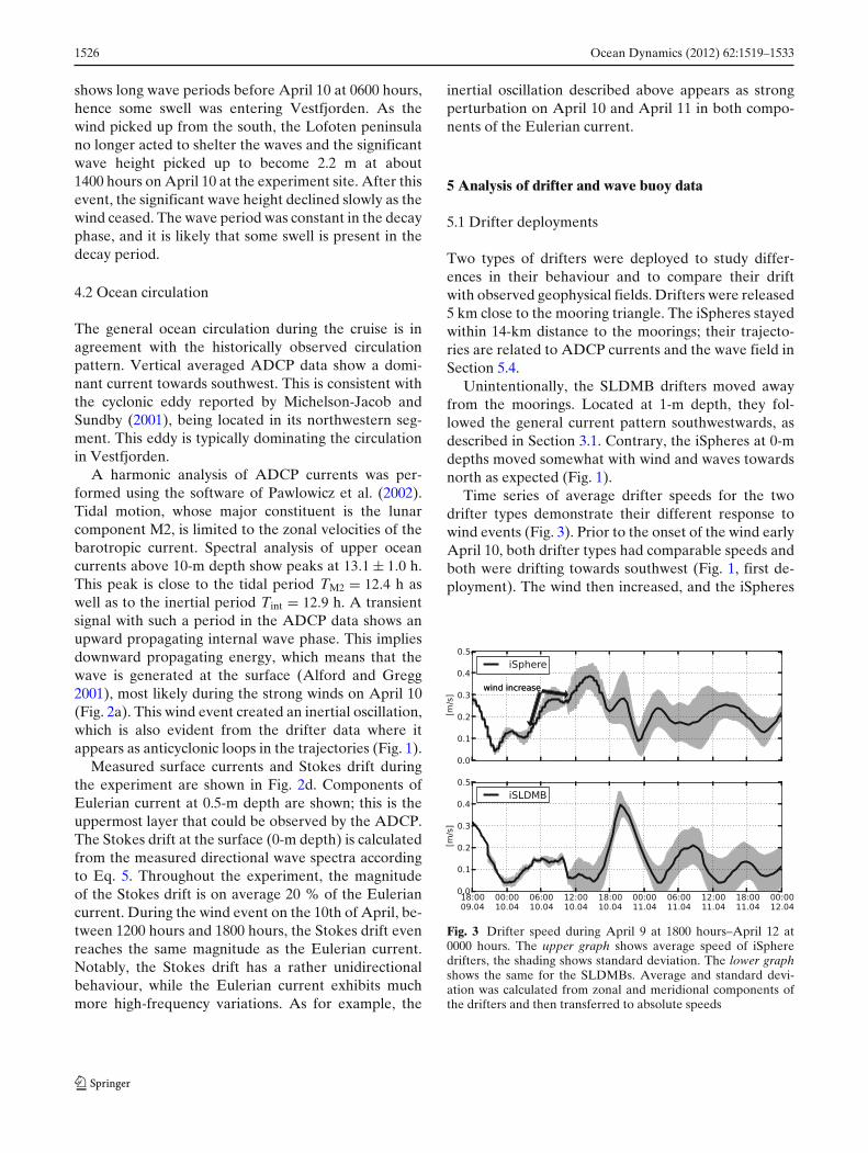
Time series of average drifter speeds for the twodrifter types demonstrate their different response towind events (Fig. 3). Prior to the onset of the wind earlyApril 10, both drifter types had comparable speeds andboth were drifting towards southwest (Fig. 1, first de-ployment). The wind then increased, and the iSpheres
Fig. 3 Drifter speed during April 9 at 1800 hours–April 12 at0000 hours. The upper graph shows average speed of iSpheredrifters, the shading shows standard deviation. The lower graphshows the same for the SLDMBs. Average and standard devi-ation was calculated from zonal and meridional components ofthe drifters and then transferred to absolute speeds
Ocean Dynamics (2012) 62:1519–1533 1527
turned rapidly and started to drift approximately inthe wind direction. The SLDMBs did not immediatelyrespond to the wind event. About 12 h later, after thewind has set up inertial currents, the SLDMBs speedwent up as well.
The second deployment included four drifters ofeach type that were released southeast of the mooringtriangle with about one nautical mile between the pairs(Fig. 1). The SLDMBs rapidly aligned along the steepslope drifting towards south-west, while the iSpheresdrifted northwards in wind and wave direction.
5.2 Structure of geophysical forcing
More details on the different behaviour of the twodrifter types were obtained from the present data. Toestimate the spatial scales of their geophysical forcingfields, we follow an analysis similarly performed byDavis (1985b), who calculated correlations betweendrifter pairs as a function of their separation.
We split up all drifter trajectories in pieces of 3 h.Correlation coefficients of simultaneous pairs of 3-htrajectories were then calculated from drifter velocities.Different from Davis’ analysis, we use the followingdefinition of a vector correlation:
r = 1 − <(vi − v j)2>
<v2i > + <v2
j>, (11)
The correlation coefficient r becomes equal to one foridentical velocities and minus one for opposite veloci-ties. Separation distances for each pair were calculatedand divided into 1-km bins. Correlation coefficients inthe same bin were averaged, yielding an average corre-lation as a function of separation. This result is shownin Fig. 4 for each drifter type separately. Some SLDMBdrifter data are available after the duration of thisexperiment because the drifters stayed in Vestfjorden.Drifter data up until the 14th of April have beenused in this analysis. Figure 4 also shows correlationsbetween SLDMB drifters and the Lagrangian currentmeasured at the mooring station, which was calculatedfrom ADCP and waverider data following Eq. 3.
Average correlations between pairs of iSpheredrifters remain above 0.8 up until 10-km separationdistance. The SLDMB drifters decorrelate rapidly inthe beginning, after only 5 km the average correlationsdrop below 0.6. The iSphere drifters stay correlated asthey separate, which indicates that their forcing exhibitslarge horizontal scales.
The iSphere drifters are located directly at the air–sea interface, their drift velocity is largely driven by
Fig. 4 Vector correlations between drifter pairs as a function ofseparation distance. The points show individual correlations andthe lines show bin averages. The blue line and the blue diamondsshow correlations between SLDMB drifters and Eulerian cur-rents measured at the mooring station, which is given by the sumof ADCP currents and the Stokes drift
wind and waves. The current further down is to a largerextent influenced by the mesoscale and submesoscalevariability of the ocean circulation, as resembled by theSLDMBs.
The SLDMBs follow the current at 1-m depth (Davis1985a); their velocities can therefore be used to in-fer statistics of the current. From the decorrelation ofSLDMB drifters, we therefore deduct that the spatialscale of the current at 1-m depth is about 5–10 km, afterwhich their average correlation drops below 0.5.
5.3 Estimated wave-induced forcing of ocean currents
In this section, we will evaluate the wave-forcing on theEulerian current. The direct effect of waves on driftersis evaluated in the next section. As with indirect waveeffect, we refer to the fact that the drifters are advectedby the Eulerian current uE, which itself is modified bywaves as described in Section 2.3.
The Eulerian current that is measured by the ADCPincludes the part of the current that is due to wave-induced surface fluxes and the Coriolis–Stokes force.An ocean model attempts to model the Eulerian cur-rent, but these wave effects are most commonly notincluded. Estimates of the wave-induced forcing havebeen obtained from measured wave spectra. The valuesof the source terms in the integrals of Eqs. 6 and 9have been calculated using the formulations given inChapter 3.3 of Komen et al. (1994). These are alsoused in the wave model WAM, as implemented at theNorwegian Meteorological Institute.
The Eulerian current is also forced by winds: the to-tal atmospheric momentum flux τ a has been calculated
1528 Ocean Dynamics (2012) 62:1519–1533
from observed wind speed and the bulk flux formulaby using the values in Smith (1988). The energy fluxesfrom wind and waves have been estimated according toEqs. 7 and 8, respectively.
In Fig. 5a, we see how the ratio between the effectiveocean surface stress τo and the total atmospheric fluxτa changes with wind and waves conditions. In risingwinds, the short wind-waves grow rapidly and a largerfraction of the atmospheric flux goes into the wave fieldinstead to the mean ocean currents. In falling winds, wesee that this situation is reversed; the low wind speedsyield a weak atmospheric flux, but the developed wavefield now provides a comparatively strong source ofmean momentum through wave dissipation processes.These results are in agreement with studies based onwave model runs (Weber et al. 2006; Saetra et al. 2007),which shows that the discrepancy between the totalatmospheric flux and the effective ocean surface stressis frequently between 20 and 30 %. In Fig. 5b, we showthe energy fluxes into and out of the wave field; theseare atmospheric fluxes transferred into wave energyand wave energy transferred to oceanic TKE. We seethat the fluxes are not perfectly balanced. The influxis larger than the outflux, hence the waves take upenergy and transport it away from the measurementlocation. Also shown is the parametrisation of Craigand Banner (1994), which is often used to model the
Fig. 5 a Momentum fluxes. The solid line shows the momentumflux into the ocean normalised by the total atmospheric flux. Thedashed line shows the wind speed. b Energy fluxes into and out ofthe wave field. The thin black line shows the parametrisation ofCraig and Banner (1994), which is frequently used to model TKEflux due to breaking waves
TKE flux to the ocean due to breaking waves. Theparametrisation is quite good, although it is better cor-related with the influx to the waves than the outfluxfrom the waves to the ocean. During the wind event, theflux of TKE to the ocean increased substantially, whichcaused increased levels of upper ocean turbulence anda deepening of the mixed layer. Such processes areimportant to model correctly as the effective eddy vis-cosity determines how momentum is distributed in thewater column and thus how the upper ocean currentsdevelop in response to external forcing by wind andwaves.
Another aspect of wave-induced forcing of theEulerian current is the Coriolis–Stokes force (Eq. 10),which is given by the Stokes drift in the upper 1 m de-rived from the measured wave spectra, Eqs. 5, and 10.The Coriolis force due to the Eulerian mean current is−ρw f k × uE. Hence, the relation between the Coriolis–Stokes force and the standard Coriolis force is given bythe relation between the Stokes drift and the Euleriancurrent. Both are shown in Fig. 2d. During strongwind and high waves, as during April 10 and 11, theCoriolis–Stokes force is as much as 80 % of the stan-dard Coriolis force. During the time scale of one inertialperiod, this might alter the direction of the upper oceancurrent by several deca-degrees as shown by Poltonet al. (2005).
5.4 Wave effects on drifter trajectories
Our observations of the Eulerian current from theADCP include the wave-forcing effects on currents thatwere described in the previous section. Additionally,surface drifters are also direct subject to the Stokesdrift. In order to evaluate the drifter trajectories interms of their forcings, we formulate a drift model thatis based on Eq. 1 and observations of Eulerian currents,waves and wind.
Because we only have Eulerian observations at onepoint, we assume horizontal constant geophysical fieldswithin 7 km around our observations. This may bejustified by the analysis in Section 5.2 which showsthat the forcing of iSphere drifters exhibit horizontalscales larger that this. Figure 4 shows that the iSpheredrifters remained highly correlated up until the sepa-ration distances of 15 km. Our iSphere drifters stayedwithin a radius of 7 km around the measurement site for2 days.
The deployment of the SLDMBs did not succeedas they immediately drifted away from the site (seeFig. 1). Spatial scales of the current that are forcingthe SLDMBs were found to be at about 5–10 km. Wecannot assume that our Eulerian measurements at 1-m
Ocean Dynamics (2012) 62:1519–1533 1529
depth are representative for a wider area. Hence, thefollowing analysis only considers the iSpheres.
5.4.1 An analytical solution of the drift equation
We evaluate the equation of motion (Eq. 1) for theiSphere drifters, neglecting the Coriolis force FC, wavescattering Fw and the drifter’s inertia, hence removingthe acceleration term. Now Eq. 1 becomes
Fa + Fo = 0, (12)
stating that the drifter motion is balanced by at-mospheric and ocean drag forces. We express the at-mospheric drag in the same way as the oceanic dragusing the wind speed U19.5 (our winds were measuredat 19.5 m high during the cruise). Since the driftervelocities are generally much smaller than the windspeed, we have approximately
Fa = 12ρa AaCa|U19.5|U19.5. (13)
From Eqs. 2, 12 and 13 we obtain
−∣∣∣∣uL − dx
dt
∣∣∣∣
(
uL − dxdt
)
= α2 |U19.5| U19.5; (14)
α =√
ρa
ρw
Aa
Aw
Ca
Cw
. (15)
The equation governing the drifter motion becomes
dxdt
= uL + αU19.5. (16)
We rederive the force balance (Eq. 14) from Eq. 16 bywriting Eq. 16 as
αU19.5 = s (17)
with s = −(uL − dxdt ). Multiplying Eq. 17 with its scalar
equivalent, i.e. α|U19.5| = |s|, yields Eq. 14.
5.4.2 Evaluation of drifter models
We will now evaluate the performance of four differentdrift trajectory models. The first is based on the forcebalance described in Section 5.4.1, while the others aresimplified versions of this model. In one model, theStokes drift will be totally neglected and another model
parameterizes the Stokes drift as a function of windvelocity. Further models neglect wind drift, using eitherthe Eulerian or Lagrangian current.
Equations 16 and 3 are used to define a “Lagrangianleeway model”, which takes observations of wind,waves and currents into account:
dxdt
= uE + uS + αU19.5, (18)
If one neglects waves, say uL ≈ uE, Eq. 18 becomes
dxdt
= uE + αU19.5 (19)
This model will be referred to as “Eulerian leewaymodel” because the drifter follows the Eulerian currentwith some wind drift.
It is possible to parameterize the Stokes drift by thewind, assuming that wind and waves are aligned andthat the wave field is in a steady state. We define sucha “Eulerian model with parameterized Stokes drift” asfollows:
dxdt
= uE + βU19.5; (20)
β = α + |us||U19.5| (21)
Here, the parameter β includes the drift by surfacewaves. The two different parameters α and β are esti-mated empirically in the following analysis. We did notcalculate α directly from Eq. 15 because the form dragcoefficients Ca and Cw are Reynolds number depen-dent and are not straightforward to use at the air–seaboundary layer with wave disturbances. Rather thanstudying this problem in detail, this study focuses onthe question which of the defined models delivers bestagreement with observations.
We estimate α by fitting Eq. 18 to the observations,this yields a best guess for the present wind drag. β isfound by fitting Eq. 20 to the observations and doesthereby implicitly include the wave drift as good aspossible. The Eulerian leeway model with wave para-metrisation is therefore the best possible attempt tomodel a drifter without wave information.
Furthermore, two models are evaluated that neglectwind drag. Equation 18 then reduces to
dxdt
= uE + uS, (22)
say the drifter simply follows the Lagrangian current;herein referred to as “Lagrangian model”. The last
1530 Ocean Dynamics (2012) 62:1519–1533
Table 2 Models for drifter velocity, wind drag parameters α (or β if applicable), and respective skill scores for different time periodsand averages for the entire experiment
Drifter velocity α / β Case a Case b Case c Case d Average
Eulerian model dx/dt = uE 0.66 0.39 0.59 0.54 0.55Lagrangian model dx/dt = uL 0.6 0.74 0.83 0.67 0.72Eulerian leeway model dx/dt = uE + αU19.5 3.1e–3 0.63 0.47 0.65 No data 0.60Eulerian leeway model with wave parametrisation dx/dt = uE + βU19.5 9.9e–3 0.56 0.65 0.74 No data 0.67Lagrangian leeway model dx/dt = uL + αU19.5 3.1e–3 0.56 0.83 0.85 No data 0.77
model, referred to as the “Eulerian model”, neglectsboth wind and waves:
dxdt
= uE (23)
All four models are summarised in Table 2. We cannow evaluate the different models based on our obser-vations. Eulerian currents are taken from the ADCPmeasurements in 0.5-m depth, which is the uppermostlayer that the ADCP could measure. The Stokes driftis obtained from the wave rider buoy using Eq. 5. Thewind is given at 19.5 m above sea surface.
With the given measurements, the drifter velocitiesof each model from Eqs. 18–23 are integrated numeri-cally with 2-min steps. The integration yields paths ofmodelled drifter trajectories, shown in Fig. 6 for an
Fig. 6 Integrated velocities of the four drifter models and theStokes drift from April 10 at 1200 hours to April 11 at 0600 hours;the black line with dots is an average path of all iSphere driftersduring this time. Starting points (red diamond) have been puttogether to compare the different paths
example period with considerably strong waves. Addi-tionally, an average path of all drifters during the sameperiod is shown. In this figure, all trajectories start atthe same point in order to compare their paths.
The models that involve wave observations (redlines) do generally show better agreement with thedrifter average (black line) than the models withoutwave information (blue and green lines), even thoughthe Eulerian leeway model with wave parametrisationincludes wave drift implicitly by a larger wind dragparameter β.
The agreement of each model with the observedtrajectories is evaluated using a separation metric thatyields a skill score for each model. As separation met-ric, the normalised cumulative Lagrangian separationsuggested by Liu and Weisberg (2011) is applied. Thisprocedure gives a separation s between a modelled anda observed trajectory:
s =∑
di/
N∑
i=0
i∑
j=0
dl j (24)
The indices i, j = 0, ..., N denominate measurementsalong a trajectory, di are distances between the mod-elled and observed positions, and dl j are distances be-tween the current and the last position on the observedtrajectory. Positions on two minute steps are used,while drifter positions are interpolated to these steps.A skill score ss is defined as
ss ={
1 − s if s ≤ 10 if s > 1
(25)
This definition of a skill score by Liu and Weisberg(2011) evaluates the entire trajectory cumulative. Highskill scores close to one mean good agreement be-tween model and observation throughout the entiretrajectory. The parameters α and β are estimated byoptimising the average skill score for all iSphere driftersduring the entire experiment from April 9 at 1800 hoursto April 12 at 0000 hours. Results are given in Table 2.
Beside average skill scores for the entire experimentand all drifters, Table 2 also shows skill scores forshorter time periods. The entire data set of iSphere
Ocean Dynamics (2012) 62:1519–1533 1531
Fig. 7 Integrated velocitiesof the Eulerian drift model,the Lagrangian drift modeland the Stokes drift for fourdifferent 18-h cases. Theblack lines with dots showstrajectories of iSpheredrifters. b and c show thesame time period withdifferent drifters
drifters is split up in 18-h periods; individual driftertrajectories for these periods are plotted in Fig. 7.
During case a, accounting for wave information doesnot enhance the model significantly as the skill score forcase a is not raised. During this period, the significantwave height is rather moderate (compare Fig. 2a), andthe integrated Stokes drift yields a rather short path(Fig. 7a). Adding wave information does not changemuch when waves are small.
During the following periods, however, waves arestronger and contribute significantly to the trajectories.Skill scores for the Eulerian model are raised from 0.55to 0.72 in the Lagrangian model, in which the Stokesdrift is added to the drifter velocity. The Eulerianleeway model with wave parametrisation takes theforward motion from waves implicitly into accountbecause an empirical parameter is used here to suitthe observations. Taking the Stokes drift properly intoaccount, which is done in the Lagrangian leeway model,still enhances the skill score from 0.67 to 0.77.
The Eulerian leeway model with wave parametrisa-tion fails if the waves are not aligned with the wind.This is the case on April 10, as shown in Fig. 2b. The
discrepancy in directions can only be accounted forwhen a wave model is used in trajectory forecasts.
It is furthermore worth to point out that theLagrangian leeway model is less sensitive to inaccura-cies in the parameters α and β because the wind dragaccounts for a smaller fraction of the drifter velocitieswhen the Stokes drift is used explicitly. The parameterβ for the Eulerian model parametrises the Stokes driftand the wind drag. The parameter α for the Lagrangianmodel only accounts for wind drag. Their differencethus represents the wave drift by wind speed. Thepresent observations show β ≈ 3α. Conclusively, theStokes drift is twice as large as the wind drag forthe used iSphere drifters.
6 Summary and concluding remarks
We have shown results from a research cruise dur-ing April 2011 in Vestfjorden, northern Norway. Theobservations include Eulerian currents, wave spectra,wind speed and direction, and drifter trajectories. Ob-
1532 Ocean Dynamics (2012) 62:1519–1533
served drift trajectories were reconstructed by driftmodels based on observations.
Drift models were formulated with and without winddrag, as well as with and without wave information.Two types of wind drag parameters were obtainedempirically: one that only accounts for the pure winddrag and one that also parametrises the Stokes drift.The trajectories of the surface drifting iSpheres werewell reconstructed by the Lagrangian mean currents,that is when wave information are used. It was shownthat the Stokes drift accounted for twice as much driftcompared to the wind drag for the given surface drifter.These results are specific for drifters located directlyat the air–sea interface. The findings from the iSpheredrifters do particularly not apply to water followingdrifters below the surface.
Wave-induced surface fluxes and the Coriolis–Stokes force could be calculated from the presentmeasurements. Their impact in terms of difference incurrent, however, could not be quantified with mea-surements because such calculations require the time-integration of the momentum equations. This can bedone with a coupled model system of waves and oceancurrents as described by Broström et al. (2008).
For the computation of the Stokes drift, we do notknow exactly how the wave buoy responds to shortwaves and how much energy that is contained in thetail of the wave spectrum. In numerical wave predictionmodels the spectral tail is parametrised. The formu-lation of the Stokes drift (Eq. 5) is proportional tothe third moment of the wave frequency spectrum andis therefore sensitive to formulation of the spectraltail.
We suggest that the predictability of drift trajectoriescan be improved by adding wave information from anumerical wave model. First of all, it is important tohave reliable estimates of the Stokes drift, which hascomparable magnitudes to the Eulerian mean currentduring strong wind events. Second, the wave-inducedfluxes of momentum and energy, and the Coriolis–Stokes force, are all significant and are likely to beimportant for the development of the Eulerian meancurrent. The drift trajectories of the submerged driftersreflect the small scale variability related to eddies, in-ertial oscillations, tides and so on. Hence, prediction ofthese trajectories strongly depends on the performanceof the ocean model.
Good estimates of the effective eddy viscosities arenecessary to realistically model the current shear andsurface velocities. Wave-induced turbulence is an activefield of research, and there is currently no consensushow such processes should be incorporated in oceanmodels. Progress in this field has to some extent been
hampered by the lack of reliable turbulence measure-ments in the upper layer of the ocean. In contrast, boththe Stokes drift, the wave dependent air–sea fluxes andthe Coriolis–Stokes force are readily included in somecurrent ocean modelling systems. All that is required isa numerical wave model that can provide the necessarydirectional wave spectra and algorithms for calculatingthe Stokes drift and the forcing fields.
The forecast skill of a numerical wave model is usu-ally on par with the skill of the atmospheric forecastmodel that provides the wind forcing. The forecastskill of ocean models is usually much lower than thisdue to small scale variability that is not properly re-solved. In particular, the ocean currents are difficultto predict. Each added wave “feature” will thereforehelp reduce the uncertainties in the prediction of drifttrajectories.
Acknowledgements We wish to thank Ilker Fer and ØyvindSætra for helpful discussions. We also gratefully acknowledgefinancial support from the Research Council of Norway throughthe grants 196438 (BioWave) and 207541 (OilWave), as well asthe Gulf of Mexico Research Initiative Deep-C Consortium. Wealso thank the Royal Norwegian Navy for supplying us with theADCP instrument, as well as Steinar Hansen from the NorwegianCoastal Administration for providing necessary logistics. We aregrateful for the constructive comments of the anonymous review-ers, who helped to increase the quality of this paper significantly.
References
Aamo OM, Jensen H (1997) Operational use of ocean surfacedrifters for tracking spilled oil. In: Proceedings of the 20thArctic and Marine Oil Spill Program (AMOP) technicalseminar, Vancouver, Canada
Alford MH, Gregg MC (2001) Near-inertial mixing: modulationof shear, strain and microstructure at low latitude. J GeophysRes 106(C8):16947–16968. doi:10.1029/2000JC000370
Ardhuin F, Marie L, Rascle N, Forget P, Roland A (2009) Obser-vation and estimation of Lagrangian, Stokes, and Euleriancurrents induced by wind and waves at the sea surface. J PhysOceanogr 39(11):2820–2838. doi:10.1175/2009JPO4169.1
Belore R, Trudel K, Morrison J (2011) Weathering, emul-sification, and chemical dispersibility of Mississippi Canyon252 crude oil: field and laboratory studies. In: 2011 interna-tional oil spill conference. Portland, Oregon
Breivik O, Allen AA (2008) An operational search and rescuemodel for the Norwegian Sea and the North Sea. J MarineSyst 69(1–2):99–113. doi:10.1016/j.jmarsys.2007.02.010
Breivik O, Allen AA, Maisondieu C, Roth J (2011) Wind-induced drift on objects at sea: the leaway field method.Appl Ocean Res 33:100–109. doi:10.1016/j.apor.2011.01.005
Broström G, Christensen KH, Weber JEH (2008) A quasi-Eulerian, quasi-Lagrangian view of surface-wave-inducedflow in the ocean. J Phys Oceanogr 38(5):1122–1130.doi:10.1175/2007JPO3702.1
Carniel S, Warner J, Chiggiato J, Sclavo M (2009) Investi-gating the impact of surface wave breaking on modeling
the trajectories of drifters in the northern Adriatic Seaduring a wind-storm event. Ocean Model 30(2–3):225–239.doi:10.1016/j.ocemod.2009.07.001
Craig PD, Banner ML (1994) Modeling wave-enhanced turbu-lence in the ocean surface layer. J Phys Oceanogr 24(12):2546–2559. doi:10.1175/1520-0485(1994)024<2546:MWETIT>2.0.CO;2
Craik ADD (1982) The drift velocity of water waves. J FluidMech 116:187–205. doi:10.1017/S0022112082000421
Craik ADD, Leibovich S (1976) Rational model forLangmuir circulations. J Fluid Mech 73:401–426. doi:10.1017/S0022112076001420
Daniel P, Jan G, Cabioc’h F, Landau Y, Loiseau E (2002)Drift modeling of cargo containers. Spill Sci Technol B7(5–6):279–288. doi:10.1016/S1353-2561(02)00075-0
Davis RE (1985a) Drifter observations of coastal surface currentsduring code: the method and descriptive view. J GeophysRes 90(C3):4741–4755. doi:10.1029/JC090iC03p04741
Davis RE (1985b) Drifter observations of coastal surface currentsduring code: the statistical and dynamical views. J GeophysRes 90:4756–4772. doi:10.1029/JC090iC03p04756
Emery W, Thomson RE (1997) Data analysis methods in physicaloceanography. Elsevier, Amsterdam
Grant ALM, Belcher SE (2009) Characteristics of Langmuirturbulence in the ocean mixed layer. J Phys Oceanogr39(8):1871–1887. doi:10.1175/2009JPO4119.1
Janssen PAEM (1989) Wave-induced stress and the drag of airflow over sea waves. J Phys Oceanogr 19:745–754
Jenkins AD (1989) The use of a wave prediction model fordriving a near-surface current model. Ocean Dyn 42:133–149. doi:10.1007/BF02226291
Jones B, Boudjelas S, Michelson-Jacob E (1997) Topographicsteering of winds in vestfjorden. Weather - London 52(10):304–311
Komen GJ, Cavaleri L, Doneland M, Hasselmann K, HasselmannS, Janssen PAE (1994) Dynamics and modelling of oceanwaves. Cambridge University Press, Cambridge
Liu Y, Weisberg RH (2011) Evaluation of trajectory model-ing in different dynamic regions using normalized cumula-tive Lagrangian separation. J Geophys Res 116(C9):C09013.doi:10.1029/2010JC006837
Longuet-Higgins MS (1953) Mass transport in water waves.Philos Trans R Soc 245:535–581
Longuet-Higgins M, Stewart R (1964) Radiation stress in waterwaves; a physical discussion with applications. Deep-Sea Res11:529–562. doi:10.1016/0011-7471(64)90001-4
Michelson-Jacob G, Sundby S (2001) Eddies of Vestfjorden,Norway. Cont Shelf Res 21(16–17):1901–1918. doi:10.1016/S0278-4343(01)00030-9
O’Donnell J, Allen A, Murphy D (1997) An assessment of the er-rors in lagrangian velocity estimates obtained by fgge driftersin the Labrador current. J Atmos Ocean Technol 14(2):
Pawlowicz R, Beardsley B, Lentz S (2002) Classical tidal har-monic analysis including error estimates in Matlab usingt_tide. Comput Geosci 28(8):929–937. doi:10.1016/S0098-3004(02)00013-4
Perrie W, Tang CL, Hu Y, DeTracy BM (2003) The impact ofwaves on surface currents. J Phys Oceanogr 33(10):2126–2140. doi:10.1175/1520-0485(2003)033<2126:TIOWOS>2.0.CO;2
Phillips OM (1977) The dynamics of the upper ocean. CambridgeUniversity Press, London
Polton JA, Lewis DM, Belcher SE (2005) The role ofwave-induced Coriolis–Stokes forcing on the wind-drivenmixed layer. J Phys Oceanogr 35(4):444–457. doi:10.1175/JPO2701.1
Rascle N, Ardhuin F (2009) Drift and mixing under theocean surface revisited: stratified conditions and model-datacomparisons. J Geophys Res 114(C2):C02016. doi:10.1029/2007JC004466
Roed L (1980) Curvature effects on hydraulically driven in-ertial boundary currents. J Fluid Mech 96(2):395–412.doi:10.1017/S0022112080002182
Smith S (1988) Coefficients for sea surface wind stress, heat flux,and wind profiles as a function of wind speed and tem-perature. J Geophys Res 93(C12)(2):311–326. doi:10.1016/0021-9991(88)90175-1
Stokes GG (1847) On the theory of oscillatory waves. TransCamb Philos Soc 8:441–473
Sundby S (1982) Fresh water budget and wind conditions. In: In-vestigations in Vestfjorden 1978. ftp://ftp.imr.no/biblioteket/files/havforsk/fh_1982_01.pdf. Accessed 21.09.2011, Fiskenog Havet, 1982: 16 s. [In Norwegian, English abstract]
Tang C, Perrie W, Jenkins A, DeTracey B, Hu Y, ToulanyB, Smith P (2007) Observation and modeling of sur-face currents on the Grand Banks: a study of the waveeffects on surface currents. J Geophys Res 112(C10):C10025.doi:10.1029/2006JC004028
Weber J, Broström G, Saetra O (2006) Eulerian vs Lagrangianapproaches to the wave-induced transport in the up-per ocean. J Phys Oceanogr 36:2106–2118. doi:10.1175/JPO2951.1
Weber J, Broström G, Christensen K (2008) Radiation stress anddepth-dependent drift in surface waves with dissipation. IntJ Offshore Polar 18(1):8–13
Weber JE (1983) Steady wind- and wave-induced currentsin the open ocean. J Phys Oceanogr 13(3):524–530.doi:10.1175/1520-0485(1983)013<0524:SWAWIC>2.0.CO;2
Weber JE, Christensen KH, Denamiel C (2009) Wave-inducedset-up of the mean surface over a sloping beach. Cont ShelfRes 29:1448–1453. doi:10.1016/j.csr.2009.03.010