Date post: | 27-Jul-2018 |
Category: |
Documents |
Upload: | phungkhanh |
View: | 217 times |
Download: | 0 times |
Observation impact in data assimilation: the effect
of non-Gaussian observation error
By ALISON FOWLER1* and PETER JAN VAN LEEUWEN2, 1Department of Mathematics,
University of Reading, Reading, UK; 2Department of Meteorology, University of Reading, Reading, UK
(Manuscript received 6 November 2012; in final form 1 May 2013)
ABSTRACT
Data assimilation methods which avoid the assumption of Gaussian error statistics are being developed for
geoscience applications. We investigate how the relaxation of the Gaussian assumption affects the impact
observations have within the assimilation process. The effect of non-Gaussian observation error (described by
the likelihood) is compared to previously published work studying the effect of a non-Gaussian prior. The
observation impact is measured in three ways: the sensitivity of the analysis to the observations, the mutual
information, and the relative entropy. These three measures have all been studied in the case of Gaussian data
assimilation and, in this case, have a known analytical form. It is shown that the analysis sensitivity can also be
derived analytically when at least one of the prior or likelihood is Gaussian. This derivation shows an
interesting asymmetry in the relationship between analysis sensitivity and analysis error covariance when the
two different sources of non-Gaussian structure are considered (likelihood vs. prior). This is illustrated for
a simple scalar case and used to infer the effect of the non-Gaussian structure on mutual information and
relative entropy, which are more natural choices of metric in non-Gaussian data assimilation. It is concluded
that approximating non-Gaussian error distributions as Gaussian can give significantly erroneous estimates of
observation impact. The degree of the error depends not only on the nature of the non-Gaussian structure, but
also on the metric used to measure the observation impact and the source of the non-Gaussian structure.
Keywords: mutual information, relative entropy, sensitivity
1. Introduction
In assimilating observations with a model, the assumptions
made about the distribution of the observation errors are
very important. This can be seen objectively by measuring
the impact the observations have on updating the estimate
of the true state, as given by the data assimilation scheme.
Many data assimilation (DA) schemes are derivable from
Bayes’ theorem, which gives the updated estimate of the
true state in terms of a probability distribution, p(xNy).
pðxjyÞ ¼ pðxÞpðyjxÞpðyÞ
(1)
In the literature, the probability distributions p(yNx),p(x) and p(xNy) are known as the likelihood, prior and
posterior, respectively. p(yNx) and p(x) must be known or
approximated in order to calculate the posterior distri-
bution, while p(y) is generally treated as a normalisation
factor as it is independent of x. The mode of the posterior
distribution is then the most likely state given all available
information and the mean is the minimum variance esti-
mate of the state.
This paper aims to give insight into how the structure of
the given distributions, p(x) and p(yNx), affect the impact
the observations have on the posterior, p(xNy). It is knownfrom previous studies that non-Gaussian statistics change
the way observations are used in data assimilation (e.g.
Bocquet, 2008). This paper presents analytical results to
explain this change in observation impact. We begin by
presenting the case of Gaussian statistics.
1.1. Gaussian statistics
An often useful approximation for p(yNx) and p(x) is that
they are Gaussian distributions, this allows the distribu-
tions to be fully characterised by a mean and covariance.
The mean of p(yNx) is the value of the observations, y,
measuring the true state and the mean of p(x) is our prior
estimate of the true state, xb. The covariances represent the
errors in these two estimates of the truth and are given by*Corresponding author.
email: [email protected]
Tellus A 2013. # 2013 A. Fowler and P. J. Van Leeuwen. This is an Open Access article distributed under the terms of the Creative Commons Attribution-
Noncommercial 3.0 Unported License (http://creativecommons.org/licenses/by-nc/3.0/), permitting all non-commercial use, distribution, and reproduction in any
medium, provided the original work is properly cited.
1
Citation: Tellus A 2013, 65, 20035, http://dx.doi.org/10.3402/tellusa.v65i0.20035
P U B L I S H E D B Y T H E I N T E R N A T I O N A L M E T E O R O L O G I C A L I N S T I T U T E I N S T O C K H O L M
SERIES ADYNAMICMETEOROLOGYAND OCEANOGRAPHY
(page number not for citation purpose)
R and B for the observations and prior estimate, respec-
tively. In the case when the observations and state are
represented in different spaces, it is necessary to transform
the likelihood into state space in order to apply Bayes’
theorem. However, if the transform is linear the likelihood
continues to be Gaussian in the observed subspace of the
state.
In assuming the likelihood and prior (and subsequently
posterior) are Gaussian the DA problem is greatly simpli-
fied. As such, these assumptions have been used in the
development of operational DA schemes for use in numeri-
cal weather prediction (NWP). For example, the Gaussian
assumption has been used in the development of variational
techniques such as 4D-Var used at the Met Office and
ECMWF (Rabier et al., 2000; Rawlins et al., 2007), and
Kalman Filter techniques such as the ensemble Kalman
filter used at Environment Canada (Houtekamer and
Mitchell, 1998). In these operational settings, a measure of
the impact of observations has been used for
� Improved efficiency of the assimilation by removing
observations with a comparatively small impact,
e.g. Peckham (1974); Rabier et al. (2002); Rodgers
(1996).
� Highlighting erroneous observations or assumed
statistics, e.g. Desroziers et al. (2009).
� Improving the accuracy of the analysis by adding
observations which should theoretically have a high
impact. For example, by defining targeted obser-
vations (Palmer et al., 1998) or the design of new
observing systems (e.g. Wahba, 1985; Eyre, 1990).
In this work we will concentrate on three measures of
observation impact: the sensitivity of the analysis (to be
defined) to the observations; mutual information; and
relative entropy. Below, these three measures are briefly
introduced and interpreted for Gaussian error statistics.
For a more in depth study of these measures see relevant
chapters within the following books: Cover and Thomas
(1991); Rodgers (2000); and Bishop (2006).
1.1.1. The sensitivity of the analysis to the observations.
In Gaussian data assimilation the mode and mean of the
posterior distribution are the same and unambiguously
define the analysis. In this case the analysis, xa, is a linear
function of the observations and prior estimate:
xa ¼ xb þ Kðy �HxbÞ; (2)
where K is known as the Kalman gain and is a function of
B, R and H. H is the observation operator, a (linear) map
from state to observation space (See Kalnay, 2003 for an
introduction to Gaussian data assimilation.)
The sensitivity of the analysis to the observations has
an obvious interpretation in terms of observation impact
(Cardinali et al., 2004). It is defined as:
S ¼ @Hxa
@y: (3)
This is a m�m matrix where m is the size of the
observation space.
From eq. (2) we can see that SG (superscript G refers to
the Gaussian assumption) is simply
SG ¼ HK: (4)
The Kalman gain can be written in many different forms
including K ¼ PGa HTR�1 where PG
a is the analysis error
covariance matrix given by
PGa ¼ ðHTR�1Hþ B�1Þ�1
: (5)
Therefore, the sensitivity is inversely proportional to R
and proportional to PGa . Hence it can be concluded from
eqs. (4) and (5), that the analysis has greatest sensitivity to
independent observations with the smallest error variance
which provide information about the region of state space
with the largest prior error.
The diagonal elements of S give the self-sensitivities and
the off-diagonal elements give the cross-sensitivities. The
trace of SG can be shown to give the degrees of freedom for
signal, ds, that is ds ¼P
i
ki, where ki is the ith eigenvalue of
HK (Rodgers, 2000).
The analysis sensitivity has proven to be a useful diag-
nostic of the data assimilation system (Cardinali et al., 2004).
It is possible to approximate eq. (4) during each analy-
sis cycle giving a valuable tool for assessing the changing
influence of observations and monitoring the validity of the
error statistics.
1.1.2. Mutual information. Mutual information is the
change in entropy (uncertainty) when the observations are
assimilated (Cover and Thomas, 1991). It is given in terms
of the prior, p(x), and posterior, p(xNy), distributions:
MI ¼Z
pðxÞ ln pðxÞdx�Z
pðyÞZ
pðxjyÞ ln pðxjyÞdxdy:
(6)
For Gaussian statistics it is unsurprisingly a function of the
analysis and background error covariance matrices, PGa and
B. In this case it is given by
MIG ¼ 1
2ln jBðPG
a Þ�1j (7)
(Rodgers, 2000), where N*N represents the determinant. As
with degrees of freedom for signal, mutual information can
be written in terms of the eigenvalues of the sensitivity
2 A. FOWLER AND P. J. VAN LEEUWEN
matrix: MI ¼ � 12
Pi
ln j1� kij. Therefore, the observa-
tions which have the greatest contribution to mutual
information should also be the observations which the
analysis is most sensitive to.
Mutual information has been used in many studies of
new observing systems. Eyre (1990) demonstrated its bene-
fits over measuring the change in error variances alone as
this measure incorporates information about the change in
the covariances too [see eq. (7)].
1.1.3. Relative entropy. Relative entropy measures the
relative uncertainty of the posterior compared to the prior
(Cover and Thomas, 1991).
RE ¼Z
pðxjyÞ ln pðxjyÞpðxÞ
dx: (8)
For Gaussian statistics it is given by
REG ¼ 1
2ðxa � xbÞ
TB�1ðxa � xbÞ þMI � 1
2ds (9)
(see Bishop, 2006). This is the only measure that depends on
the value of the analysis, xa, and so is sensitive not only to
how the covariance of the analysis error is affected by the
observations but also how the observations affect the actual
value of the analysis. Therefore the observations which
result in the greatest relative entropy do not necessarily give
the largest mutual information or analysis sensitivity if the
signal term in eq. (9), 12ðxa � xbÞ
TB�1ðxa � xbÞ, is dominant.
However, in a study of the measures, ds, MI and RE by
Xu et al. (2009), it was found that for defining an optimal
radar scan configuration the result had little dependence on
which of these measures were used.
Relative entropy has received little attention in opera-
tional DA due to its dependence on the observation values.
However, the shift in the posterior away from the prior, not
just the reduction in uncertainty, is clearly an important
aspect of observation impact. For this reason, this measure
has been included in our current study.
1.2. Non-Gaussian statistics
Although Gaussian data assimilation has proven to be a
powerful tool, in some cases a Gaussian distribution gives a
poor description of the error distributions. For example,
it is found that describing the observation minus back-
ground differences (known as innovations) as a Gaussian
distribution often underestimates the probability of extreme
innovations (the tails are not fat enough) and so the
associated observations are assumed to be unlikely rather
than providing valuable information about extreme
events, and so removed in quality control. Following on
from Ingleby and Lorenc (1993), non-Gaussian likelihoods
such as the Huber function (Huber, 1973), are being used
in operational quality control to make better use of the
available observations. Another study of innovation statis-
tics performed by Pires et al. (2010) found significant
deviations fromGaussian distributions in the case of quality
controlled observations of brightness temperature from
the High Resolution Infrared Sounder (HIRS). Pires et al.
(2010) concluded that incorrectly assuming Gaussian sta-
tistics can have a large impact on the resulting estimate of
the state. In this case, the magnitude of the effect on the
estimate of the state was seen to depend upon the size of the
innovation and the non-Gaussian structure in the likelihood
relative to that in the prior.
From eq. (1), we see that there are no restrictions on
our choice of p(yNx) or p(x) when calculating the posterior
and the more accurately these distributions are defined the
more accurate our posterior’s representation of our knowl-
edge of the state will be. This simple fact has led to a recent
surge in research into non-Gaussian DA methods which are
applicable to the geosciences, see van Leeuwen (2009) and
Bocquet et al. (2010) for a review of a range of possible
techniques.
This work follows on from Fowler and van Leeuwen
(2012), in which the effect of a non-Gaussian prior on the
impact of observations was studied when the likelihood
was restricted to a Gaussian distribution. The main con-
clusions from that paper are summarised below.
In Fowler and van Leeuwen (2012) a Gaussian mixture
was used to describe the prior distribution to allow for a
wide range of non-Gaussian distributions. It was shown
that, in the scalar case, the sensitivity of the analysis to
observations was still given by the analysis error variance
divided by the observation error variance as in the Gaussian
case [see eq. (4)]. However, the sensitivity could become a
strong function of the observation value because the
analysis error variance is no longer independent of the
observation value. Therefore, when the prior and observa-
tion error distributions are fixed but the position of the
likelihood, given by the observation value, is allowed to
change, the analysis is most sensitive to observations which
also result in the largest analysis error variance. This is not a
desirable property for a measure of observation impact.
Fowler and van Leeuwen (2012) concluded that comparing
the analysis sensitivity to the sensitivity when a Gaussian
prior was assumed eq. (4), showed that the Gaussian assum-
ption could lead to both a large overestimation and a large
underestimation depending on the value of the observation
relative to the background and the structure of the prior.
The error in the Gaussian approximation to relative
entropy was also seen to give a large range of errors as a
function of the observation value relative to the back-
ground.However, for a particular realisation of the observa-
tion value, the errors in the Gaussian approximation to
OBSERVATION IMPACT IN DATA ASSIMILATION 3
relative entropy and the Gaussian approximation to the
sensitivity did not necessarily agree in sign or magnitude.
This highlighted the fact that care is needed when making
conclusions about the influence of a non-Gaussian prior on
the observation impact.
Mutual information is independent of the realisation of
the observation error [as seen in eq. (6)] and so as a measure
of the influence of a non-Gaussian prior it provides a more
consistent result. Mutual information was also seen in
Fowler and van Leeuwen (2012) to be affected a relatively
small amount by a non-Gaussian prior.
To summarise: allowing for non-Gaussian prior statistics
has a significant effect on the observation impact. The
choice of metric is more important than in the Gaussian
case as the consistency between the different measures
breaks down.
Within this current paper we shall compare these pre-
vious findings to the case when it is the likelihood that is
non-Gaussian. A non-Gaussian prior or likelihood may
result from the properties of the state variable. For
example, if the variable has physical bounds then we
know, a priori, that the probability of the variable being
outside of these bounds is zero which is inconsistent with
the infinite support of the Gaussian distribution. This is a
particular issue when the variable is close to these bounds.
The non-Gaussian prior may also result from a non-linear
forecast providing our prior estimate of the state. In this
case a wide variety of non-Gaussian distributions are possi-
ble and techniques such as the particle filter (van Leeuwen,
2009) allow for the non-linear model to implicitly give the
prior distribution. A non-Gaussian likelihood may similarly
result from a non-linear map between the observation and
state space. However, within this paper we shall only give
consideration to linear observation operators. Non-linear
observation operators greatly complicate the problem,
as not only do they create non-Gaussian likelihoods out
of Gaussian observation errors, the structure of the non-
Gaussian PDF depends on the value of the observation.
The observation error in this case is defined as:
E ¼ y �Hxtruth
Possible contributing factors to E include:
� Random error associated with the measurement.
� Random errors in the observation operator, for
example due to missing processes or linearisation.
This is often distinguished from representivity error
which deals with the additional error source due to
the observations sampling scales which the model is
unable to resolve (Janjic and Cohn, 2006).
� Systematic errors are also possible, which may have
synoptic, seasonal or diurnal signals some of which
can be corrected. There are also gross errors which
need to be identified and rejected by quality control
(e.g. Gandin et al., 1993; Qin et al., 2010; Dunn
et al., 2012).
These sources of random error could all potentially lead to
a non-Gaussian structure in the observation errors. Errors
associated with the observation operator will in general be
state dependent (Janjic and Cohn, 2006). For this reason,
within this paper, we will focus on the case of perfect linear
observation operators so that the non-Gaussian structure
is a characteristic of the instrument error or pre-processing
of the observations before they are assimilated. It is
assumed that this error source is independent of the state.
In analysing the impact of the non-Gaussian likelihood
(rather than a non-Gaussian prior) we shall follow a similar
methodology to that in Fowler and van Leeuwen (2012).
We shall first derive some general results for the sensitivity
of the analysis to the observations. We will then look at
a scalar example when the likelihood is described by a
Gaussian mixture with two components each with identical
variances, GM2. This will allow for direct comparison to
the results in Fowler and van Leeuwen (2012). Finally
we will look at the case when the measurement error is
described by a Huber function which cannot be described
well by the GM2 distribution.
2. The effect of non-Gaussian statistics on the
analysis sensitivity
In non-Gaussian data assimilation the analysis must be
explicitly defined. In this work we define the analysis as
the posterior mean giving the minimum variance estimate
of the state rather than the mode which can be ill-defined
when the posterior is multi-modal. In extreme bimodal
cases this does lead to the possibility of the analysis having
low probability.
The sensitivity of the analysis to the observations can be
calculated analytically when either the prior or likelihood
is Gaussian, see appendix A. It can be shown that in the
case of an arbitrary likelihood and Gaussian prior that the
sensitivity is given by
SnGpðyjxÞ ¼ @Hla
@y¼ Im �HPaB
�1HTðHHTÞ�1(10)
where ma is the analysis (mean of the posterior). When the
likelihood is Gaussian, Pa ¼ PGa ¼ ðB�1 þHTR�1HÞ�1
and
the expression given in eq. (10) is equal to HK [see Section
1.1.1, eq. (4)]. However, a non-Gaussian likelihood means
that Pa becomes a function of the observation value and
hence the sensitivity is also a function of the observation
value.
From eq. (10) it is seen that SnGpðyjxÞ increases as Pa
decreases and so for a fixed prior and likelihood structure,
4 A. FOWLER AND P. J. VAN LEEUWEN
the realisation of y for which the analysis has maximum
sensitivity also gives the smallest analysis error covariance.
In other words, the analysis is most sensitive to observa-
tions which improve its accuracy.
This is in contrast to when the prior is non-Gaussian and
the likelihood is Gaussian. In this case the sensitivity is
given by (see Appendix A)
SnGpðxÞ ¼ @Hla
@y¼ HPaH
TR�1: (11)
This has the same form as eq. (4) in Section 1.1.1. In this
case, it is seen that SnGpðxÞ is proportional to the analysis
error covariance. Therefore for a fixed prior and likelihood
structure, the analysis is most sensitive to observations
which reduce its accuracy.
The analysis error covariance is an important aspect in
DA in which it is desirable to find a minimum value.
Therefore, from eqs. (10) and (11), we can conclude that
the influence of a non-Gaussian likelihood on the analysis
sensitivity is of a fundamentally different nature to the
influence of a non-Gaussian prior. This is demonstrated for
a simple scalar example in the next section.
3. A simple example
For comparison to the results in Fowler and van Leeuwen
(2012) in which the effect of a skewed and bimodal prior on
the observation impact was studied we shall look at the
scalar case when the likelihood can be described by a
Gaussian mixture with two components each with identical
variance, GM2.
pðyjxÞ ¼ðð2pÞr2Þ�12 w exp �ðyþ n1 � xÞ2
2r2
( )
þ ð1� wÞ exp �ðyþ n2 � xÞ2
2r2
( )�:
(12)
In this example it is assumed that we have direct observa-
tions of the state, x, and so the observation operator, H,
is simply the identity. From eq. (12) we see that as a
function of x, the means of the Gaussian components are
l1 ¼ yþ n1 and l2 ¼ yþ n2. To ensure that eq. (12) is non-
biased, i.e.Rðy� xÞpðyjxÞdx ¼ 0, we have the constraint
wn1 þ ð1� wÞn2 ¼ 0, effectively making our observation,
y, the mean of the likelihood. This could be restrictive,
particularly in the case of a strongly bimodal likelihood
when the observation would have a low probability. How-
ever, as long as the observation value is chosen to be the
likelihood mean plus a constant, the analysis sensitivity
presented below remains unchanged.
The likelihood in eq. (12) is described by four para-
meters: the relative weight of the Gaussian components, w,
the means of the Gaussian components, m1 and m2, and
the variance of the Gaussian components, s2. These four
parameters give rise to a large variety of non-Gaussian
distributions, this can be seen from expressions for the
skewness and kurtosis.
The variance of the likelihood, p(yNx) as a function
of x, is:
r2y ¼ r2 þ wð1� wÞðl1 � l2Þ
2:
Using this expression for the variance we can give the
following expression for the skewness of p(yNx):
w3y ¼
Rðx� lyÞ
3pðyjxÞdx
r3y
¼ wð1� wÞð1� 2wÞðl1 � l2Þ3
r3y
:
And the kurtosis of p(yNx):
j4y ¼
Rðx� lyÞ
4pðyjxÞdx
r4y
� 3
¼ ðl1 � l2Þ4wð1� wÞð1� 6wþ 6w2Þ
r4y
The values of skewness and kurtosis are plotted in Fig. 1 as
a function of w and m2�m1 when s2�1. It is clear that for a
fixed value of m2�m1, the skewness increases as Nw�0.5Nincreases until it reaches a maximum (indicated by the
dotted line in Fig. 1), then the skewness sharply returns to
zero as Nw�0.5N approaches 0.5 and GM2 returns to a
Gaussian distribution. When the weights are equal (w�0.5)
only negative values of kurtosis are possible, increasing as
m2�m1 increases. This results in a likelihood with a flatter
peak than the Gaussian distribution becoming bimodal as
w(1�w)(m1�m2)2 exceeds s2. Positive values of kurtosis are
possible when the distribution is also highly skewed. Note
that a Gaussian distribution has zero kurtosis.
Non-Gaussian structure such as skewness could result
from bounds on the observed variable or as a result of non-
linear pre-processing. In such a case it should be possible
to construct a model of the errors associated with the
measurement, such as the GM2 distribution introduced in
this section, through comparison to other observations and
prior information for which we have a good estimate of
the errors. It is difficult to think of a situation when the
likelihood may be strongly bimodal without accounting for
a non-linear observation operator. For example, an ambi-
guity in the observation could result in a bimodal error
such as in the use of a scatterometer to measure wind
direction from waves (Martin, 2004). Modelling y�NxNresults in a likelihood with a GM2 distribution with equal
weights, if the error on the observation, y, is Gaussian.
In this case the means of the two Gaussian components
would be m1�y and m2��y. However, the general results
provided in Section 2 do not hold. As such in the following
OBSERVATION IMPACT IN DATA ASSIMILATION 5
analysis the emphasis is not on the extreme bimodal case
but the smaller deviations from a Gaussian distribution
that the GM2 distribution allows.
Whentheprior isgivenbyaGaussian pðxÞ ¼ NðlGx ; kr2Þð Þ,
the posterior will also be given by a GM2 distribution
[refer to Bayes’ theorem, eq. (1)] with updated parameters.
These updated parameters are given by
~w ¼ we�a1
we�a1 þ ð1� wÞe�a2
; (13)
where ai ¼ ððli � lGx Þ
2Þ=ð2ð1þ kÞr2Þ.
~li ¼kli þ lG
x
1þ k;
for i�1,2.
~r2 ¼ kr2
1þ k:
Note that these have the same form as in Fowler and van
Leeuwen (2012) due to the symmetry of Bayes’ theorem.
Given this expression for the posterior distribution we
can calculate its mean as: la ¼ ~w el1 þ ð1� ~wÞ el2. The sen-
sitivity of the posterior mean to the observations can then
be expressed in terms of the parameters of the likelihood
distribution as:
SGM2pðyjxÞ¼ @la
@y¼ k
k þ 1� kwð1� wÞðl1 � l2Þ
2e�a1�a2
ð1þ kÞ2r2ðwe�a1 þ ð1� wÞe�a2Þ2:
(14)
This expression has a striking resemblance to the sensitivity
in the case of the non-Gaussian prior, SGM2pðxÞ. In eq. (13)
of Fowler and van Leeuwen (2012), when the prior has the
same form as the likelihood described in eq. (12), SGM2pðxÞ
was shown to be
SGM2pðxÞ ¼ 1
jþ 1þ jwð1� wÞðl1 � l2Þ
2e�a1�a2
ð1þ jÞ2r2ðwe�a1 þ ð1� wÞe�a2Þ2: (15)
In this case pðyjxÞ ¼ Nðy; jr2Þ and ai �((y � mi)2)/
ð2ð1þ jÞr2Þ. Note the distinction between k and j; theseparameters are used to define the ratio of the Gaussian
variances to the Gaussian component variance for the non-
Gaussian likelihood case and the non-Gaussian prior case,
respectively.
An example of the setup of this simple scalar example is
shown in Fig. 2. In the left-hand panel the non-Gaussian
prior case which was the focus of Fowler and van Leeuwen
(2012) is illustrated and in the right-hand panel the non-
Gaussian likelihood case is illustrated. The values of k and
j have been chosen such that r2y=r
2x is fixed in the two
setups, where r2y is the variance of the likelihood (either
Gaussian or not) and r2x is the variance of the prior (which
also may or may not be Gaussian).
We see in eq. (14) that the sensitivity tends towards an
upper bound of kkþ1
as the likelihood becomes Gaussian
(m1�m2 tends to zero) with no lower bound when the like-
lihood has two distinct modes (i.e. ðl1 � l2Þ2=r2 is large).
In contrast, in eq. (15), the sensitivity tends towards a lower
bound of 1jþ1
as the prior becomes Gaussian with no upper
bound when the prior has two distinct modes. The lack of
lower and upper bounds for the non-Gaussian likelihood
case and non-Gaussian prior case, respectively, has an
important consequence for the analysis error variance.
From the relationship between the sensitivity and posterior
variance given in Section 2 we can conclude that when
SGM2pðyjxÞB0 that r2a > r2
x and similarly when SGM2pðxÞ > 1
that r2a > r2
y. In theory this should never be the case for
0 0.2 0.4 0.6 0.8 1
0.5
1
1.5
2
2.5
3
3.5
4
−1
−0.8 −
0.8
−0.6 −0
.6
−0.4
00
0
−0.4
−0.
4
−02
−0.2
−0.2
−0.
2 0.20.2
0.2
020.4
0.4
0.4
0.6
0.6
0.8 0.8
1
0
0
0
w
µ 2−µ 1
skewness
0 0.2 0.4 0.6 0.8 1
0.5
1
1.5
2
2.5
3
3.5
4 −1
−1
−0.5
−0.5
−0.
505
0.5
0.5 0.5
0.5
05
1
1 1
1
1.5
1.5
2 2
00
0
00
0
w
µ2−
µ1
kurtosis
Fig. 1. Skewness (left) and kurtosis (right) of the GM2 distribution as a function of w and m2�m1 when s2�1.
6 A. FOWLER AND P. J. VAN LEEUWEN
purely Gaussian data assimilation. The potential for the
analysis error variance to be greater than the observation
and prior error variances was similarly demonstrated
for the case of errors following an exponential law in
Talagrand (2003) and when a particle filter is used to
assimilate observations with a non-linear model of the
Agulhas Current in van Leeuwen (2003).
As a function of the innovation, d�y�mx, the shape of
SGM2pðyjxÞ is similar to SGM2pðxÞ although inverted. In each
case the sensitivity is a symmetrical function of d about a
central value. In the non-Gaussian likelihood case, this
value of d, d1, marks a minimum value of SGM2pðyjxÞ. In the
non-Gaussian prior case, this value of d, dp, marks a
maximum value of SGM2pðxÞ. In general dl 6¼ dp unless all
parameters are identical with w�1/2. Away from d1 and dpthe sensitivity tends to k
kþ1for the non-Gaussian likelihood
case and 1jþ1
for the non-Gaussian prior case, as could
be expected from the symmetry between k and 1=j. When
the parameters describing the non-Gaussian distribution
are the same, the relative speed at which the sensitivity
asymptotes to kkþ1
or 1jþ1
depends on the values of k and j,
respectively, if k ¼ j then it is the same.
An example of this is shown in Fig. 3, where s2�1,
w�0.25, m1�m2�3 for both the non-Gaussian likelihood
and non-Gaussian prior. j ¼ 2 for comparison to the
example in Fowler and van Leeuwen (2012) and k is
chosen to be 1849/512 so that in each case the Gaussian
approximation to the sensitivity is the same, that is SG ¼r2
xðr2x þ r2
y�1
stays constant even though r2x and r2
y are not
identical in the two cases, in fact the error variances for the
prior and likelihood are larger in the non-Gaussian like-
lihood case than in the non-Gaussian prior case (see Fig. 2).
From eq. (12) and (13) k > j implies that SGM2pðyjxÞ is a
broader function of d (thin blue line) than SGM2pðxÞ (thin
black line) and there is less variance in the sensitivity. This
illustrates, that unlike the Gaussian case, the sensitivity is
now dependent on the actual values of the error variances
rather than just their ratio. The Gaussian approximation to
the sensitivity, SG, is given by the bold dashed line.
As NdN increases ~w tends to 0/1 in both cases, in effect
rejecting one of the modes. In other words the posterior
asymptotes to a Gaussian with variance given by ~r2 ¼ kr2
1þk
in the case of a non-Gaussian likelihood and ~r2 ¼ jr2
1þj in the
case of a non-Gaussian prior. This explains why the
sensitivity, which is given by eq. (10) in the non-Gaussian
likelihood case and by eq. (11) in the non-Gaussian prior
case, tends to a non-zero constant value as NdN increases. It
also explains (with some extra thought) why in the non-
Gaussian likelihood case this constant sensitivity is greater
than the Gaussian approximation and vice versa when the
prior is non-Gaussian.
The value of d, which results in a peak value of SGM2pðxÞ,
was given in Fowler and van Leeuwen (2012) in terms of
the parameters of the non-Gaussian prior.
dp ¼1
2ðl1 � l2Þl2
1 � l22 � 2ð1þ jÞr2 ln
w
ð1� wÞ
!" #� lx:
(16)
We may similarly find an expression for d1, which results
in a minimum value of SGM2pðyjxÞ, when the likelihood is
Fig. 2. Schematic of experimental setup in section 3. Left hand panel: Non-Gaussian prior and Gaussian likelihood as in Fowler and
van Leeuwen (2012). Right hand panel: Non-Gaussian likelihood and Gaussian prior, which is the focus of this paper. In each case the
non-Gaussian parameters are given by w ¼ 0:25, r2 ¼ 1, jl1 � l2j ¼ 3. The variance of the Gaussian distributions are chosen such that in
each case r2y=r
2x ¼ 32
43, for agreement with Fowler and van Leeuwen (2012), giving k�1849/512 and j ¼ 2.
OBSERVATION IMPACT IN DATA ASSIMILATION 7
non-Gaussian. From eq. (10) we know that as the sen-
sitivity increases the analysis error variance decreases.
Therefore when the posterior is of the same form as eq.
(12), the posterior variance is at a maximum, and hence the
sensitivity is at a minimum, when the posterior weights are
equal, i.e. the posterior is symmetric. This insight allows us
to find the observation value for which the analysis has
least sensitivity by finding the d which satisfies ~w ¼ 0:5.
dl ¼1
2ðl2 � l1Þðl2 � l1Þ
2ð1� 2wÞ þ 2r2ð1þ kÞ ln 1� w
w
� �(17)
Note that in deriving eq. (17) we have made use of the fact
that for d ¼ y� lGx ¼ l2 � wðl2 � l1Þ � lG
x the terms lGx ,
w and m1�m2 are considered to be fixed. Therefore we only
need to find an expression for m2 which satisfies ~w ¼ 0:5.
This can then be substituted back into the expression for d.
When the weights are equal in the non-Gaussian prior
(i.e. w ¼ 12) dp�0. Similarly when w ¼ 1
2in the non-
Gaussian likelihood, dl ¼ 0. Therefore, when the prior is
symmetric but with negative kurtosis the analysis is
most sensitive when the mean of the (Gaussian) likelihood
is equal to the mean of the prior. Conversely when the
likelihood is symmetric but with negative kurtosis the
analysis is least sensitive when the mean of the likelihood
is equal to the mean of the (Gaussian) prior.
The results illustrated by the example of Fig. 3 can be
shown for a range of non-Gaussian distributions described
by eq. (12). In Fig. 4, contour plots of SGM2pðyjxÞ=SG (left
column) and SGM2pðxÞ=SG (right column) are given as a
function of d and m2�m1 (top row) and w (bottom row).
In all cases k and j are varied such that SG remains the
same value as in Fig. 3. In practice this means that as the
variance of the non-Gaussian distribution is increased as
a result of the parameters describing the distribution
changing, the variance of the Gaussian distribution is
similarly increased. Indicated in Fig. 4 is the increasing
negative kurtosis as l2 � l1 increases and the increasing
skewness as jw� 0:5j increases, see Fig. 1 for comparison.
As expected the error in the Gaussian approximation to
the sensitivity becomes larger as the skewness and kurtosis
of the likelihood/prior increases. The magnitude of the
error in the Gaussian approximation to the sensitivity is
larger when the prior is non-Gaussian, because in this
case SG > 0:5 leading to a narrower function of sensitivity
than when the likelihood is non-Gaussian, as explained
previously. If SGB0:5 then the error in the Gaussian
approximation to the sensitivity would be larger when the
likelihood is non-Gaussian. The gradient in the maximum/
minimum sensitivity as a function of w (see Figs. 2c and 2d)
can be derived from eqs. (16) and (17).
3.1. Comparison of sensitivity to other measures of
observation impact
The focus of Fowler and van Leeuwen (2012) was to
compare the effect of a non-Gaussian prior on different
measures of observation impact. It was seen that like the
−15 −10 −5 0 5 10 15
0.4
0.5
0.6
0.7
0.8
0.9
1
d
sens
itivi
tynon Gaussian priornon−Gaussian likelihood1/(κ +1)k/(k+1)Gaussian approxdp
dl
Fig. 3. Comparison of S ¼ @la
@yas a function of d when the likelihood is non-Gaussian (prior is Gaussian) (thin blue line) and when the
prior is non-Gaussian (likelihood is Gaussian) (thin black line). In each case the non-Gaussian distribution is a two component Gaussian
mixture with identical variances with parameter values as in Fig. 2. The variance of the Gaussian distributions, also given in Fig. 2, are
chosen such that the Gaussian estimate to the sensitivity is the same in each case (bold, dashed line). Also marked on is kkþ1
(bold blue line)
and 1jþ1
(bold black line), and dp (black dashed line) and dl (blue dashed line).
8 A. FOWLER AND P. J. VAN LEEUWEN
sensitivity, the error in the Gaussian approximation to
relative entropy was a strong function of the innovation.
The strong dependence of both the error in the sensitivity
and the error in the relative entropy on the innovation
means that there is no consensus as to the effect of a non-
Gaussian prior on the observation impact for a given
observation value. A similar conclusion can be arrived at
when the likelihood is non-Gaussian by comparing Figs. 4a
and 4c to 5a and 5c, in which fields of S=SG and RE=REG
have been plotted, respectively.
Relative entropy [see eq. (8)] is loosely related to the
sensitivity in two ways:
(1) As seen when relative entropy was first introduced,
relative entropy is dependent on the shift of the
posterior distribution away from the prior. The shift
of the posterior distribution away from the prior,
given by la � lx, is proportional to the sensitivity of
ma to y due to the following relationship:
@Hla
@yþ @Hla
@Hlx
¼ Im; (18)
where Im is an identity matrix of size m (see
Appendix A).
As a function of d, the error in the Gaussian
approximation to the shift in the posterior away
from the prior will be smallest when la � lx. This
is only approximate because, unlike in the purely
Gaussian case, y ¼ lx does not necessarily imply that
la ¼ lx In Fowler and van Leeuwen (2012) this was
wrongly assumed to be true. However, as seen in the
example given in Fig. 3, the sensitivities are almost
equal to the Gaussian approximation of the sensitivity
at d�0. Therefore when y ¼ lx, ma is very close to mxwhen either the prior or likelihood is non-Gaussian.
Away from this the Gaussian approximation will
underestimate the shift when it underestimates the
sensitivity and similarly overestimate the shift when it
overestimates the sensitivity.
(2) Relative entropy also measures the reduction in the
uncertainty between the prior and posterior. This is
strongly linked to the posterior variance: the larger
the posterior variance the smaller the reduction in
uncertainty. The sensitivity’s relationship to the poste-
rior error variance is given by eqs. (10) and (11).
Therefore when the likelihood is non-Gaussian the
reduction in uncertainty is overestimated when the
sensitivity is overestimated and when the prior is
−10 −5 0 50.5
1
1.5
2
2.5
3
3.5
4
0.8 0.9
1.1
1.11.2
1.21.3
1.31.4
1.4
1
1
d
µ 2−µ 1
a) S/SG− nonG likelihood
−10 −5 0 50.5
1
1.5
2
2.5
3
3.5
4
0.5 0.5
0.60.6
0.7
0.70.8
0.8
0.9 0.9
1.1
1.1
1.2
1.3
1.41.5
1
1d
µ 2−µ 1
b) S/SG− nonG prior
−10 −5 0 5
0.2
0.4
0.6
0.8 0.6
0.6
0.7
0.7
0.8
0.8
0.9
0.9
0.9
0.9
1.1
1.11.1
1.2
1.2
1.2
1.2
1.3
1.3
1.3
1.3
1.4
1.4
1
1
1
1
d
w
c) S/SG− nonG likelihood
−10 −5 5
0.2
0.4
0.6
0.8 0.6
0.6
0.6
0.6
0.7
0.7
0.7
0 7
0.8 0.
8
0.9
0.9
1.1
1.1
1.2
1.21.3
1.3
1.4
1.4
1.5
1.5
1 1
d
w
d) S/SG− nonG prior
−vekurtosis
+veskewness
−veskewness
Fig. 4. Comparison of S normalised by its Gaussian approximation when the likelihood is non-Gaussian (prior is Gaussian) (a, c) and
when the prior is non-Gaussian (likelihood is Gaussian) (b, d). In the top two panels the effect of separating the Gaussian components
(y-axis) is given when the weights are equal. In the bottom two panels the effect of varying the weights of the Gaussian components (y-axis)
is given when jl1 � l2j ¼ 3. In all cases s2�1 and r2y=r
2x is kept constant at 32
43by varying the values of k and j.
OBSERVATION IMPACT IN DATA ASSIMILATION 9
non-Gaussian the reduction in uncertainty is under-
estimated when the sensitivity is overestimated.
These two comments explain why in Fowler and van
Leeuwen (2012) it was found that the error in relative
entropy was generally of a smaller magnitude than the
error in sensitivity as the two processes above cancel to
some degree. It also explains why in this case, when it is the
likelihood that it is non-Gaussian, that the error in relative
entropy is generally of a greater magnitude than the error
in sensitivity as the two processes above reinforce each
other to some degree. This can be seen by comparing Figs.
4 and 5.
These two comments also explain the asymmetry in the
error in relative entropy as a function of d when w 6¼ 12[see
Figs. 5c and 5d]. When w 6¼ 12the minimum in error in the
shift of the posterior at d � 0 does not coincide with the
maximum (minimum) in the reduction in the posterior
variance at d ¼ dpðlÞ.
Because of the large variability in the sensitivity and
relative entropy as a function of observation value it is
useful to look at their averaged values,R
pðyÞSdy andRpðyÞREdy. The latter is known as mutual information,
a measure of the change in entropy when an observation
is assimilated (see Section 1.1.1 and Cover and Thomas,
1991).
On average the Gaussian approximation to the non-
Gaussian likelihood underestimates the observation impact
[see Figs. 6a and 6c]. This is because the Gaussian estimate
of the likelihood underestimates the structure and hence the
information in the likelihood. This is analogous to the non-
Gaussian prior case presented in Fowler and van Leeuwen
(2012) where on average the Gaussian approximation to
the non-Gaussian prior overestimated the observation
impact due to it underestimating the structure in the prior
(see Figs. 6b and 6d).
As expected from mutual information’s relation to
relative entropy and consequently relative entropy’s rela-
tion to the sensitivity, the error in the Gaussian approxi-
mation to MI is greater than the error in the Gaussian
approximation toR
pðyÞSdy when the true likelihood is
non-Gaussian and vice versa when it is the prior that is
non-Gaussian.
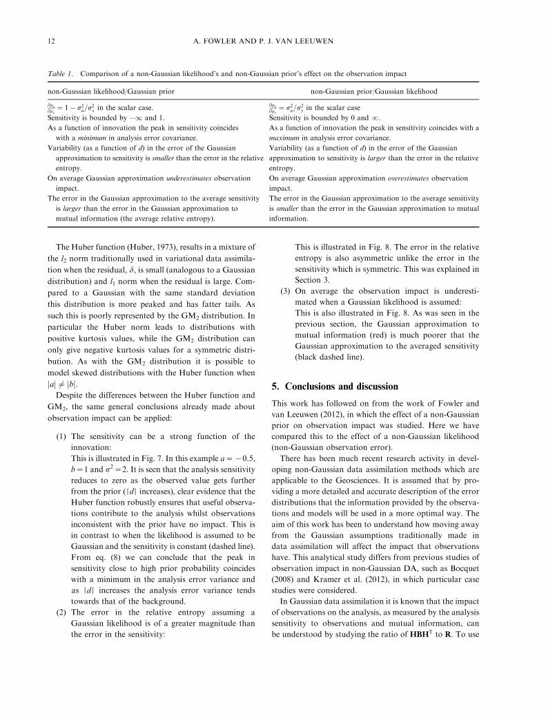
A summary of some of the key differences between
observation impact when the likelihood and prior are non-
Gaussian, as discussed in this Section are given in Table 1.
In this section we have studied the observation impact
when a non-Gaussian distribution as described by a two-
component Gaussian mixture with identical variances,
given by eq. (10), is introduced. This has allowed us to
understand how the source of non-Gaussian structure
affects the different measures of observation impact when
−10 −5 0 50.5
1
1.5
2
2.5
3
3.5
4
0.9
1.1
1.11.2
1.2
1.3
1.3
1.4
1.4
1.5 1.5
1
1
d
µ 2−µ 1
a) RE/REG− nonG likelihood
−10 −5 0 50.5
1
1.5
2
2.5
3
3.5
4
0.8 0.8
0.9
0.9
1.1 1.1
1
1
1
1
d
µ 2−µ 1
−10 −5 0 5
0.2
0.4
0.6
0.8 0.7
0.7
0.8
0.8
0.9
0.9
1.1
1.11.1
1.2
1.2
1.3
1.3
1.4
1.4
1.4
1.4
1.5
1.5
1.6
1.6
1
1
1
1
d
w
c) RE/REG− nonG likelihood
−10 −5 0 5
0.2
0.4
0.6
0.80.8
0.8
0.8
0.8
0.9 0.
9
1.1
1.1
1.1
1.1
1.2
1.2
1
1
11
d
w
d) RE/REG− nonG prior
b) RE/REG− nonG prior
−vekurtosis
+veskewness
−veskewness
Fig. 5. As in Fig. 4 but for RE.
10 A. FOWLER AND P. J. VAN LEEUWEN
the distributions are skewed or have non-zero kurtosis.
At the ECMWF, a mixed Gaussian and exponential
distribution, known as a Huber function, has recently
been introduced to model the observation error for some
in-situ measurements (Tavolato and Isaksen, 2009/2010)
during quality control. In the next section we will give a
brief overview of the observation impact in this specific
case.
4. The Huber function
The Huber function has been shown to give a good fit to
the observation minus background differences seen in
temperature and wind data from sondes, wind profilers,
aircrafts, and ships (Tavolato and Isaksen, 2009/2010).
From non-Gaussian observation minus background diag-
nostics it is difficult to derive the observations error
structure alone (Pires et al., 2010). However, due to the
difficulty in designing a data assimilation scheme around
non-Gaussian prior errors, it is a pragmatic choice to
assign the non-Gaussian errors to the observations only.
The Huber function is described by the following
pðyjxÞ ¼
1
rffiffiffiffi2pp expða2
2� jadjÞ if dBa
1
rffiffiffiffi2pp expð� 1
2d2Þ if a � d � b
1
rffiffiffiffi2pp expðb2
2� jbdjÞ if d > b
8><>: ; (19)
where d ¼ y�HðxÞr ¼ d=r. The distribution is therefore char-
acterised by the following four parameters: y, the observa-
tion value, s2; the variance of the Gaussian part of the
distribution; and the parameters a and b which define the
region and the extent of the exponential tails. Therefore as
a and b are increased the Huber function relaxes back to a
Gaussian distribution.
0.2 0.4 0.6 0.80.5
1
1.5
2
2.5
3
3.5
4
µ 2−µ 1
w
0.2 0.4 0.6 0.80.5
1
1.5
2
2.5
3
3.5
4
µ 2−µ 1
w
b) MI/MIG− nonG priora) MI/MIG− nonG likelihood
0.2 0.4 0.6 0.80.5
1
1.5
2
2.5
3
3.5
4
µ 2−µ 1
w
0.2 0.4 0.6 0.80.5
1
1.5
2
2.5
3
3.5
4
µ 2−µ 1
w
d) average S/SG− nonG priorc) average S/SG− nonG likelihood
Fig. 6. Top: Comparison of MI normalised by its Gaussian approximation as a function of w (x axis) and m2�m1 (y axis) when (a) the
likelihood is non-Gaussian (prior is Gaussian) and (b) when the prior is non-Gaussian (likelihood is Gaussian). Bottom: Comparison ofRpðyÞSdy normalised by its Gaussian approximation as a function of w (x axis) and l2 � l1 (y axis) when (c) the likelihood is non-Gaussian
(prior is Gaussian) and (d) when the prior is non-Gaussian (likelihood is Gaussian). In all cases s2�1 and r2y=r
2b is kept constant at 32
43by
varying the values of k and j. Red contours indicate values above 1 and blue contours indicate values below one. The contours are
separated by increments of 0.02.
OBSERVATION IMPACT IN DATA ASSIMILATION 11
The Huber function (Huber, 1973), results in a mixture of
the l2 norm traditionally used in variational data assimila-
tion when the residual, d, is small (analogous to a Gaussian
distribution) and l1 norm when the residual is large. Com-
pared to a Gaussian with the same standard deviation
this distribution is more peaked and has fatter tails. As
such this is poorly represented by the GM2 distribution. In
particular the Huber norm leads to distributions with
positive kurtosis values, while the GM2 distribution can
only give negative kurtosis values for a symmetric distri-
bution. As with the GM2 distribution it is possible to
model skewed distributions with the Huber function when
jaj 6¼ jbj.Despite the differences between the Huber function and
GM2, the same general conclusions already made about
observation impact can be applied:
(1) The sensitivity can be a strong function of the
innovation:
This is illustrated in Fig. 7. In this example a��0.5,
b�1 and s2�2. It is seen that the analysis sensitivity
reduces to zero as the observed value gets further
from the prior (NdN increases), clear evidence that the
Huber function robustly ensures that useful observa-
tions contribute to the analysis whilst observations
inconsistent with the prior have no impact. This is
in contrast to when the likelihood is assumed to be
Gaussian and the sensitivity is constant (dashed line).
From eq. (8) we can conclude that the peak in
sensitivity close to high prior probability coincides
with a minimum in the analysis error variance and
as NdN increases the analysis error variance tends
towards that of the background.
(2) The error in the relative entropy assuming a
Gaussian likelihood is of a greater magnitude than
the error in the sensitivity:
This is illustrated in Fig. 8. The error in the relative
entropy is also asymmetric unlike the error in the
sensitivity which is symmetric. This was explained in
Section 3.
(3) On average the observation impact is underesti-
mated when a Gaussian likelihood is assumed:
This is also illustrated in Fig. 8. As was seen in the
previous section, the Gaussian approximation to
mutual information (red) is much poorer that the
Gaussian approximation to the averaged sensitivity
(black dashed line).
5. Conclusions and discussion
This work has followed on from the work of Fowler and
van Leeuwen (2012), in which the effect of a non-Gaussian
prior on observation impact was studied. Here we have
compared this to the effect of a non-Gaussian likelihood
(non-Gaussian observation error).
There has been much recent research activity in devel-
oping non-Gaussian data assimilation methods which are
applicable to the Geosciences. It is assumed that by pro-
viding a more detailed and accurate description of the error
distributions that the information provided by the observa-
tions and models will be used in a more optimal way. The
aim of this work has been to understand how moving away
from the Gaussian assumptions traditionally made in
data assimilation will affect the impact that observations
have. This analytical study differs from previous studies of
observation impact in non-Gaussian DA, such as Bocquet
(2008) and Kramer et al. (2012), in which particular case
studies were considered.
In Gaussian data assimilation it is known that the impact
of observations on the analysis, as measured by the analysis
sensitivity to observations and mutual information, can
be understood by studying the ratio of HBHT to R. To use
Table 1. Comparison of a non-Gaussian likelihood’s and non-Gaussian prior’s effect on the observation impact
non-Gaussian likelihood/Gaussian prior non-Gaussian prior/Gaussian likelihood
@la
@ly¼ 1� r2
a=r2x in the scalar case. @la
@ly¼ r2
a=r2y in the scalar case
Sensitivity is bounded by �1 and 1. Sensitivity is bounded by 0 and �.
As a function of innovation the peak in sensitivity coincides
with a minimum in analysis error covariance.
As a function of innovation the peak in sensitivity coincides with a
maximum in analysis error covariance.
Variability (as a function of d) in the error of the Gaussian
approximation to sensitivity is smaller than the error in the relative
entropy.
Variability (as a function of d) in the error of the Gaussian
approximation to sensitivity is larger than the error in the relative
entropy.
On average Gaussian approximation underestimates observation
impact.
On average Gaussian approximation overestimates observation
impact.
The error in the Gaussian approximation to the average sensitivity
is larger than the error in the Gaussian approximation to
mutual information (the average relative entropy).
The error in the Gaussian approximation to the average sensitivity
is smaller than the error in the Gaussian approximation to mutual
information.
12 A. FOWLER AND P. J. VAN LEEUWEN
relative entropy to measure the observation impact, it is
also necessary to know the values of the observation and
the prior estimate of the state. When the assumption of
Gaussian statistics are relaxed we have shown that the
impact of the observations on the analysis becomes much
more complicated and a deeper understanding of the metric
used to measure the impact as well as the source of the non-
Gaussian structure is necessary.
We have shown that there exists an interesting asymme-
try in the relationship of the analysis sensitivity to the
analysis error covariance between the two sources of non-
Gaussian structure. This means that relaxing the assump-
tion of a Gaussian likelihood has a very different effect on
observation impact, as given by this metric, than relaxing
the assumption of a Gaussian prior. The sensitivity’s
dependence upon the analysis error variance only also
−40 −20 0 20 40−0.2
0
0.2
0.4
0.6
0.8
1
d
sens
itivi
ty
non−Gaussian likelihoodGaussian
−40 −30 −20 −10 0 10 200
0.05
0.1
0.15
x
p(x)
likelihoodpriory=−19.4
Fig. 7. Left: Huber likelihood (black) a ¼ �0:5, b�1 and s2�2, when ly ¼ �19:4. Gaussian prior (blue), mx�0, variance of prior
chosen such that for the variance of the full likelihood (r2y not s2) r2
y=r2x is 32/43. Right: The sensitivity of the analysis to the observation.
−40 −20 0 20 40
0
0.5
1
1.5
2
2.5
d
MI/MIG
S/SG
RE/REG
average S/SG
Fig. 8. Mutual information (red), sensitivity (black), relative entropy (blue) and the average sensitivity (black dashed) all normalised by
their Gaussian approximations plotted as a function of d.
OBSERVATION IMPACT IN DATA ASSIMILATION 13
means that it does not measure the full influence of the
observations and may erroneously indicate a degradation of
the analysis due to the assimilation of the observations.
From this we can conclude that the sensitivity of the
analysis to the observations is no longer a useful measure
of observation impact when non-Gaussian errors are con-
sidered. However the fact that it is possible to derive
analytically its relationship with the analysis error covar-
iance, has helped to give us insight into the different effects
the two sources of non-Gaussian structure have on relative
entropy and mutual information. These measures are much
more suitable in the case of non-Gaussian error statistics
because they take into account the effect of the observations
on the full posterior distribution whilst still having a clear
physical interpretation. Mutual information has the added
benefit that it is independent of the observation value,
and so provides a consistent measure of the observation
impact as an experiment is repeated. It is also always
positive by construction and so will always measure an
improvement in our estimate of the state when observations
are assimilated. However, as a consequence mutual infor-
mation is more difficult to measure in non-Gaussian data
assimilation because it involves averaging over observation
space.
We have illustrated these findings in the case when the
non-Gaussian distribution is modelled by a two component
Gaussian mixture. This has allowed for an analytical study
of the effect of increasing the skewness and bimodality
on observation impact, and has helped to emphasise the
differing effect of the source of the non-Gaussian structure
on observation impact. The key conclusions from this
analytical study have been shown to be applicable to other
non-Gaussian distributions such as the Huber function.
The work presented here has been restricted to the case
when the map between observation and state space is
linear. However, there are many observation types which
are not linearly related to state variables, for example,
satellite radiances are a non-linear function of temperature,
humidity, etc., throughout the depth of the atmosphere.
In this case, even if the observation error were Gaussian,
a non-linear observation operator would result in a non-
Gaussian likelihood in state space. The results shown in
this paper are not directly applicable to this source of
non-Gaussianity, as the structure of the likelihood function
in state space is now dependent on the observation value.
This makes an analytical study much more difficult as
shown in appendix A.3. A study of the effect of a non-
linear observation operator is left for future work.
6. Acknowledgements
This work has been funded by the National Centre for
Earth Observation (NCEO) part of the Natural Environ-
ment Research Council (NERC), project code H5043718,
and forms part of the ‘ESA Advanced Data Assimilation
Methods’ project, contract number ESRIN 4000105001/11/
I-LG. We would also like to thank Carlos Pires and two
anonymous reviewers for their valuable comments.
7. Appendix
A.1. The sensitivity of the analysis mean to the
likelihood mean
Bayes’ theorem states that the probability of the state, x,
given information y can be derived from the prior prob-
ability of x and the likelihood.
pðxjyÞ ¼ pðxÞpðyjxÞpðyÞ
: (20)
where pðyÞ ¼R
pðxÞpðyjxÞdx.
The analysis can be given by the mean of the posterior,
la ¼Z
xpðxjyÞdx: (21)
Substituting eqs. (20) into (21) we see that the analysis is
only dependent on the observation value through the like-
lihood, p(yNx). The sensitivity of the analysis in observation
space to the observation value, y ¼ lyðþconstÞ, is then
given by
@Hla
@ly
¼
RHxpðxÞ @pðyjxÞ
@lydxR
pðxÞpðyjxÞdx�Hla
RpðxÞ @pðyjxÞ
@lydxR
pðxÞpðyjxÞdx: (22)
Recall that H is the (linear) operator which transforms a
vector from state to observation space.
It is also of interest to look at the sensitivity of the analysis
to the mean of the prior, lx, in observation space. In this
case it is only the prior, p(x), in eq. (20) which is sensitive to
lx and so the sensitivity of the analysis to the mean of the
prior is given by
@Hla
@Hlx
¼R
HxpðyjxÞ @pðxÞ@Hlx
dxRpðxÞpðyjxÞdx
�Hla
RpðyjxÞ @pðxÞ
@HlxdxR
pðxÞpðyjxÞdx: (23)
In the following subsections we will show that it is possible
to evaluate these sensitivities when either the prior or
likelihood are Gaussian.
A.2. Non-Gaussian prior, Gaussian likelihood
Let p(x) be arbitrary and p(yNx) be Gaussian with mean
lyand error covariance R.
pðyjxÞ ¼ ðð2pÞmjRjÞ�12 exp � 1
2ðly �HxÞTR�1ðly �HxÞ
� �:
(24)
14 A. FOWLER AND P. J. VAN LEEUWEN
Here m is the size of observation space. Therefore
@pðyjxÞ@ly
¼ �pðyjxÞðly �HxÞTR�1: (25)
A.2.1. Analysis sensitivity to observations. Equation (25)
can be substituted into eq. (22) to give
@Hla
@ly
¼ �Hla lTy R�1 þ
ZHxxTHTR�1pðxjyÞdx
þHlalTy R�1 �Hlal
Ta HTR�1: (26)
Note thatR
xxTpðxjyÞdx� lalTa is the analysis error
covariance matrix, Pa. eq. (26) therefore simplifies to
@Hla
@ly
¼ HPaHTR�1: (27)
A.2.2. Analysis sensitivity to background. In calculating
the sensitivity with respect to the background (the mean of
the prior), in this case, we do not have access to @pðxÞ@Hlx
.
However we do know @pðxÞ@Hlx¼ � @pðxÞ
@Hxas the change in the
probability caused by perturbing the value of x is the same
as perturbing lx by the same magnitude but in the opposite
direction. Therefore we can utilise integration by parts, that
is,R
u @v@x
dx ¼ uv �R@u@x
vdx.
First evaluate the first term of eq. (23):
Let u ¼ HxpðyjxÞand @v@x¼ @pðxÞ
@Hx. Therefore @u
@x¼ HpðyjxÞðInþ
xðly �HxÞTR�1HÞ. v can be found by noting @pðxÞ@x
HT ¼@pðxÞ@Hx
@Hx@x
HT, it then follows that v ¼ pðxÞHTðHHTÞ�1.R
HxpðyjxÞ @pðxÞ@Hlx
dx ¼ �R
HxpðyjxÞ @pðxÞ@Hx
dx
¼ � pðyjxÞpðxÞHxHTðHHTÞ�1h i1
�1þR
pðyjxÞpðxÞHðInþ xðly �HðxÞTÞR�1HÞHTðHHTÞ�1dx:
(28)
The first term of eq. (23) is then
Im þHlalTy R�1 �H
ZpðxjyÞxxTdxHTR�1: (29)
Likewise we may evaluate the second term of eq. (23):
Let u ¼ pðyjxÞ and @v@x¼ @pðxÞ
@Hlxagain. Therefore
@u@x¼ ðly �HðxÞÞTR�1HpðyjxÞ and v is unchanged.ZpðyjxÞ @pðxÞ
@Hlx
dx ¼ �Z
pðyjxÞ @pðxÞ@Hx
dx
¼ � pðyjxÞpðxÞHTðHHTÞ�1h i1
�1
þZðly �HðxÞÞTR�1HpðyjxÞpðxÞHTðHHTÞ�1
dx:
(30)
The second term of eq. (23) is then
�HlalTy R�1 þHlal
Ta HTR�1: (31)
It then follows that
@Hla
@Hlx
¼ Im �HPaHTR�1 (32)
A.3. Non-Gaussian likelihood, Gaussian prior
Let p(yNx) be arbitrary and p(x) be Gaussian with mean
lxand error covariance B.
pðxÞ ¼ ðð2pÞpjBjÞ�12 exp � 1
2ðlx � xÞTB�1ðlx � xÞ
� �: (33)
Therefore
@pðxÞ@Hlx
¼ �pðxÞðlx � xÞTB�1HTðHHTÞ�1: (34)
A.3.1. Analysis sensitivity to observations. The derivation
of @Hla
@lyis analogous to the derivation of @Hla
@Hlxin the previous
section, as @pðyjxÞ@ly
in this case is unknown and so we must
make use of integration by parts.
It can be shown that in this case
@Hla
@ly
¼ Im �HPaB�1HTðHHTÞ�1(35)
A.3.2. Analysis sensitivity to background. The derivation
of @Hla
@Hlxis analogous to the derivations of @Hla
@lyin the previous
section as @pðxÞ@lx
in this case is known.
@Hla
@Hlx
¼ HPaB�1HTðHHTÞ�1: (36)
From this we can conclude that when either the prior or
likelihood is Gaussian it is always the case that:
@Hla
@ly
þ @Hla
@Hlx
¼ Im (37)
A.4. Non-linear observation operator
Following a similar methodology as in Appendix A.2 and
A.3, the analysis sensitivity to the observations when the
OBSERVATION IMPACT IN DATA ASSIMILATION 15
observation operator is non-linear, represented by h(x), can
be shown to be
@hðlaÞ@ly
¼ H
ZxðhðxÞÞTR�1pðxjyÞdx
��la
ZðhðxÞÞTR�1pðxjyÞdx
�;
(38)
where H is the observation operator linearised about
the analysis. In this expression it has been assumed that
the likelihood in observation space is Gaussian, i.e.
y � Nðly;RÞ but no assumptions about the prior have
been necessary. When h(x) is non-linear there is no longer a
clear relationship between the sensitivity and the analysis
error covariance matrix.
References
Bishop, C. 2006. Pattern Recognition and Machine Learning.
Springer Science�Business Media, LLC, New York.
Bocquet, M. 2008. Inverse modelling of atmospheric tracers:
non-gaussian methods and second-order sensitivity analysis.
Nonlinear Process. Geophys. 15, 127�143.Bocquet, M., Pires, C. A. and Wu, L. 2010. Beyond gaussian
statistical modeling in geophysical data assimilation. Mon. Wea.
Rev. 138, 2997�3023.Cardinali, C., Pezzulli, S. and Andersson, E. 2004. Influence-
matrix diagnostics of a data assimilation system. Q. J. Roy.
Meteorol. Soc. 130, 2767�2786. DOI: 10.1256/qj.03.205.
Cover, T. M. and Thomas, J. A. 1991. Elements of Information
Theory (Wiley Series in Telecommunications). John Wiley,
New York.
Desroziers, G., Berre, L., Chabot, V. and Chapnik, B. 2009.
A posteriori diagnostics in an ensemble of perturbed analyses.
Mon. Wea. Rev. 137, 3420�3436.Dunn, R. H. J., Willet, K. M., Thorne, P. W., Woolley, E. V.,
Durre, I. and co-authors. 2012. HadISD: a quality-controlled
global synoptic report database for selected variables at long-
term stations from 1973�2011. Clim. Past. 8, 1649�1679.Eyre, J. E. 1990. The information content of data from satellite
sounding systems: a simulation study. Q. J. Roy. Meteorol. Soc.
116, 401�434. DOI: 551.501.7:551.507.362.2.
Fowler, A. M. and van Leeuwen, P. J. 2012. Measures of obser-
vation impact in non-gaussian data assimilation. Tellus. 64, 17192.
Gandin, L. S., Monrone, L. L. and Collins, W. G. 1993. Two years
of operational comprehensive hydrostatic quality control at the
national meteorological center. Weather. Forecast. 57, 57�72.Houtekamer, P. L. and Mitchell, H. L. 1998. Data assimilation
using an ensemble kalman filter technique. Mon. Wea. Rev. 126,
798�811.Huber, P. J. 1973. Robust regression: asymptotics, conjectures,
and monte carlo. Ann. Stat. 1, 799�821.Ingleby, B. and Lorenc, A. 1993. Bayesian quality control using
multivariate normal distributions. Q. J. Roy. Meteorol. Soc. 119,
1195�1225.
Janjic, T. and Cohn, S. 2006. Treatment of observation error due
to unresolved scales in atmospheric data assimilation. Mon.
Wea. Rev. 134, 2900�2915.Kalnay, E. 2003. Atmospheric Modeling, Data Assimilation and
Predictability. Cambridge University Press, New York.
Kramer, W., Dijkstra, H. A., Pierini, S. and van Leeuwen, P. J.
2012. Measuring the impact of observations on the predictability
of the kuroshio extension in a shallow-water model. J. Phys.
Oceanogr. 42, 3�17.Martin, S. 2004. An Introduction to Ocean Remote Sensing.
Cambridge University Press, Cambridge pp.
Palmer, T. N., Gelaro, R., Barkmeijer, J. and Buizza, R. 1998.
Singular vectors, metric, and adaptive observations. J. Atmos.
Sci. 55, 633�653.Peckham, G. 1974. The information content of remote measure-
ments of the atmospheric temperature by satellite ir radiometry
and optimum radiometer configurations. Q. J. Roy. Meteorol.
Soc. 100, 406�419.Pires, C. A., Talagrand, O. and Bocquet, M. 2010. Diagnosis and
impacts of non-gaussianity of innovations in data assimilation.
Pysica. D. 239, 1701�1717.Qin, Z.-K., Zou, X., Li, G. and Ma, X.-L. 2010. Quality control of
surface station temperature data with non-gaussian observation-
minus-background distributions. J. Geophys. Res. 115. DOI:
10.1029/2009JD013695.
Rabier, F., Fourrie, N., Chafai, D. and Prunet, P. 2002. Channel
selection methods for infrared atmospheric sounding interfe-
rometer radiances. Q. J. Roy. Meteorol. Soc. 128, 1011�1027.Rabier, F., Jarvinen, H., Klinker, E., Mahfouf, J.-F. and
Simmons, A. 2000. The ECMWF operational implementation
of four-dimensional variational data assimilation. I: experimen-
tal results and simplified physics. Q. J. Roy. Meteorol. Soc. 126,
1143�1170.Rawlins, F., Ballard, S. P., Bovis, K. J., Clayton, A. M., Li, D. and
co-authors. 2007. The Met Office global four-dimensional varia-
tional data assimilation scheme. Q. J. Roy. Meteorol. Soc. 133,
347�362.Rodgers, C. D. 1996. Information content and optimisation of high
spectral resolution measurements. Proc. SPIE. 2830, 136�147.Rodgers, C. D. 2000. Inverse Methods for Atmospheric Sounding.
World Scientific, Singapore pp.
Talagrand, O. 2003. Bayesian Estimation. Optimal Interpolation.
Statistical Linear Estimation in Data Assimilation for the Earth
System, Volume 26 of NATO Science Series IV Earth and
Environmental Sciences. Springer, Netherlands.
Tavolato, C. and Isaksen, L. Huber norm quality control in the
IFS. ECMWF Newsletter No. 122, 2009/2010.
van Leeuwen, P. J. 2003. A variance-minimizing filter for large-
scale applications. Mon. Wea. Rev. 131, 2071�2084.van Leeuwen, P. J. 2009. Particle filtering in geophysical systems.
Mon. Wea. Rev. 137, 4089�4114.Wahba, G. 1985. Design criteria and eigensequence plots for satellite-
computed tomography. J. Atmos. Oceanic. Technol. 2, 125�132.Xu, Q., Wei, L. and Healy, S. 2009. Measuring information
content from observations for data assimilation: connection
between different measures and application to radar scan design.
Tellus. 61A, 144�153.
16 A. FOWLER AND P. J. VAN LEEUWEN