NOAA Technical Memorandum ERL PMEL-31

OBSERVATIONS OF SOUTH ALASKAN COASTAL WINDS

R. M. ReynoldsS. A. MacklinT. R. Hiester

Pacific Marine Environmental LaboratorySeattle, WashingtonJuly 1981

UNITED STATESDEPARTMENT OF COMMERCE

Malcolm Baldrige.Secnllary

NATIONAL OCEANIC ANDATMOSPHERIC ADMINISTRATION

John V. Byrne,Administrator

Environmental ResearchLaboratories

George H. LudwigDirector

NOTICE

The Environmental Research Laboratories do not approve, recommend, norendorse any proprietary product or proprietary material mentioned in thispublication. No reference shall be made to the Environmental ResearchLaboratories or to this publication furnished by the Environmental ResearchLaboratories in any advertising or sales promotion which would indicate orimply that the Environmental Research Laboratories approve, recommend, orendorse any proprietary product or proprietary material mentioned herein,or which has as its purpose an intent to cause directly or indirectly theadvertised product to be used or purchased because of this EnvironmentalResearch Laboratories publication.

ii

FiguresTablesAbstract

CONTENTS

ivvi

1

1 . INTRODUCTION 11.1 Survey of Coastal Wind Types 11.2 Offshore Modification of Coastal Winds 4

2. MEASUREMENTS OF COASTAL WINDS IN ALASKA 52.1 Instruments and Analysis 52.2 Weather Patterns Over the South Alaskan Coast 122.3 Observations at the Malaspina Glacier 16

3. CONCLUSION 45

4. REFERENCES 48

iii

Figures

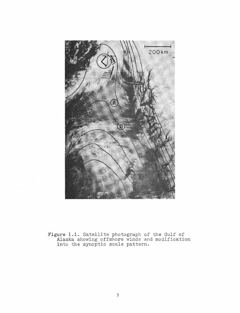
1.1 Satellite photograph of the Gulf of Alaska show­ing offshore winds and modification into thesynoptic scale pattern. 3

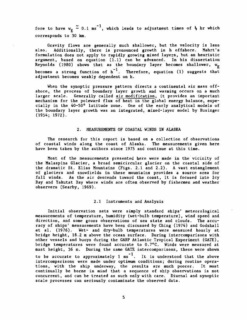
2.1 A Lambert conformal projection of the MalaspinaGlacier showing elevations in feet. Shaded areassuggest the limit of the glacier. 6

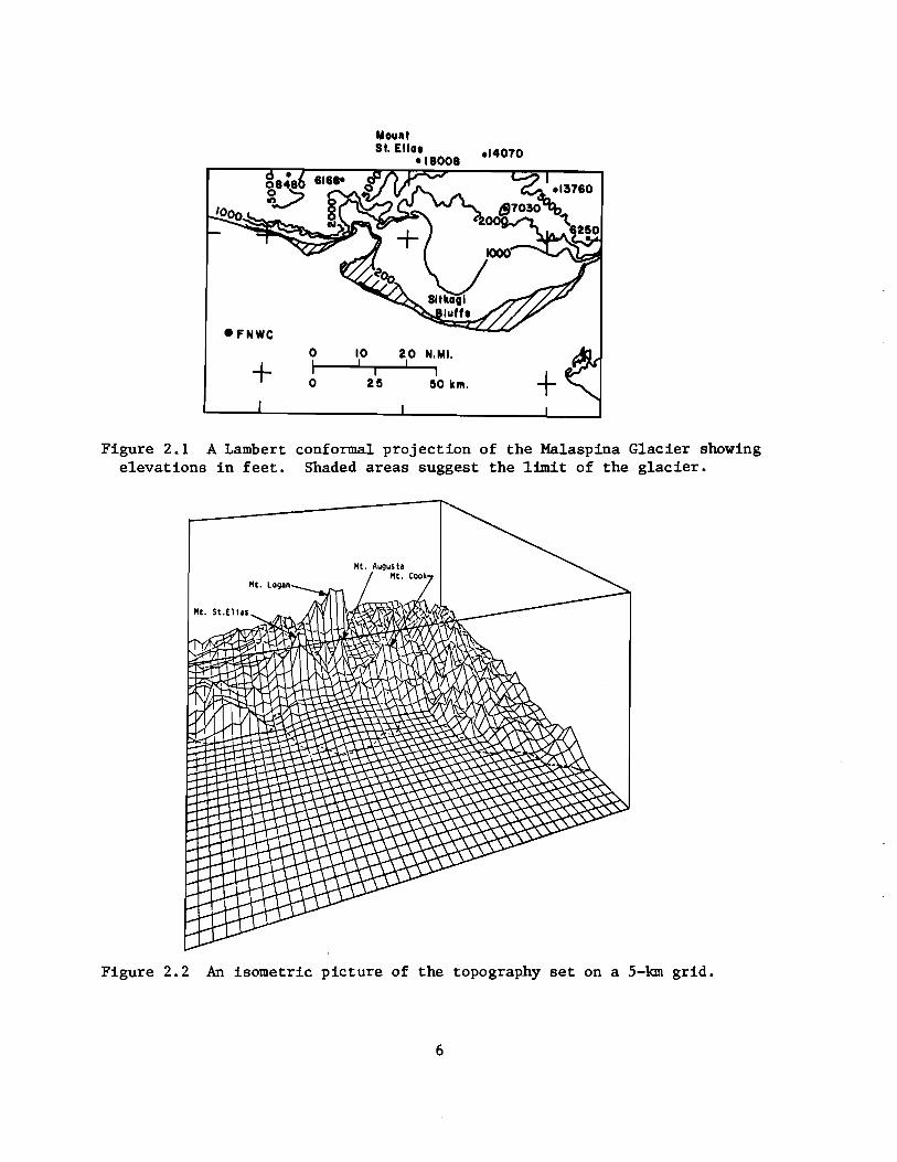
2.2 An isometric picture of the topography set on a5-km grid. 6

2.3 Same map as Figure 2.1 showing positions ofmeteorological stations used in this study. 8

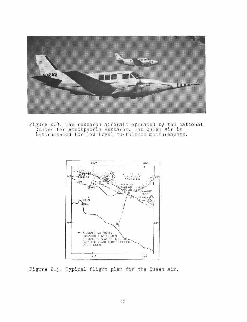
2.4 The research aircraft operated by the NationalCenter for Atmospheric Research. The Queen Airis instrumented for low level turbulence meas-urements. 10

2.5 Typical flight plan for the Queen Air. 10

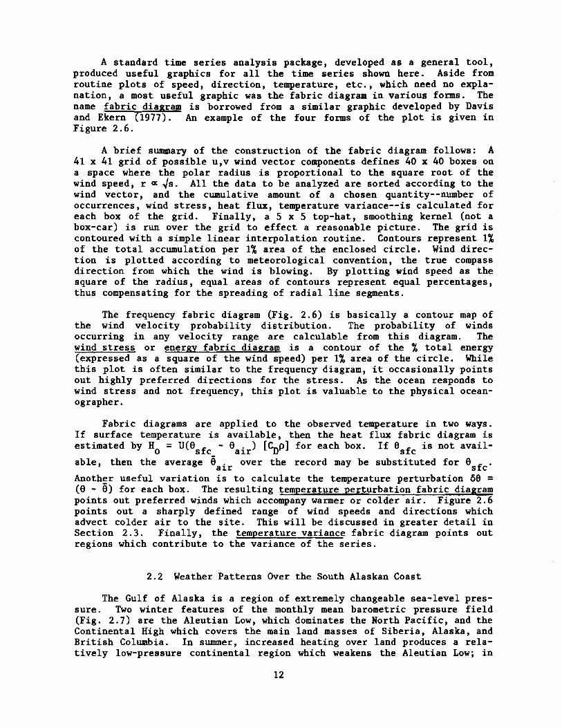
2.6 (a) Typical fabric diagrams of wind frequencyand energy. The data is from EB43 for the per-iod of 6 March to 3 April 1977. 13(b) Fabric diagrams of temperature perturbationand variance for the same data as 2.6(a). 14

2.7 Average meteorological conditions in the Gulf ofAlaska for various months of the year. Solidarrows are principal storm tracks, dashedarrows are secondary tracks. (From Searby,1969). 15

2.8 (a) (b) Most common synoptic scale types asclassified by Putnins (1966). Classificationsymbol and percentage of occurance are shownin the upper right hand corners. 17

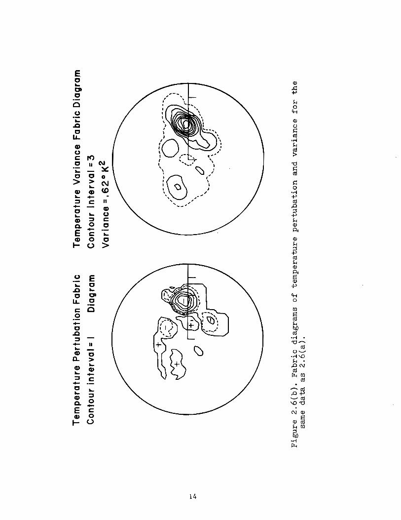
2.8 (c)(d) Most common synoptic scale types asclassified by Putnins (1966). Classificationsymbol are percentage of occurance are shown inthe upper right corners. 18

2.9 (a) Fabric diagrams of wind observations atEB33 compared with those £ymputed by FNWC. Thecircle repre!ints a 30 ms wind, and ticks mark10 and 20 ms speed. 20

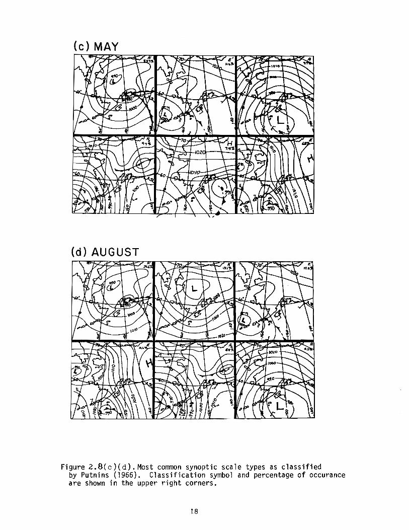
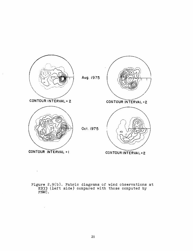
2.9 (b) Fabric diagrams of wind observations atEB33 (left side) compared with those computedby FNWC. 21

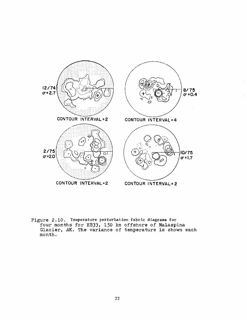
2.10 Temperature perturbation fabric diagrams forfour months for EB33, 150 km offshore ofMalaspina Glacier, AK. The variance of tem-perature is shown each month. 22

iv

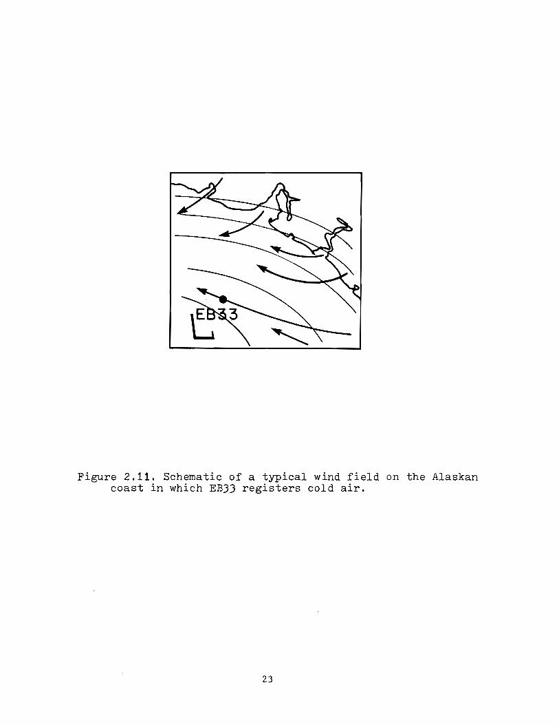
2.11 Schematic of a typical wind field on the Alaskancoast in which EB33 registers cold air. 23

2.12 Time series of wind speed and direction ascomputed by FNWC for the two time periods ofinterest. 24

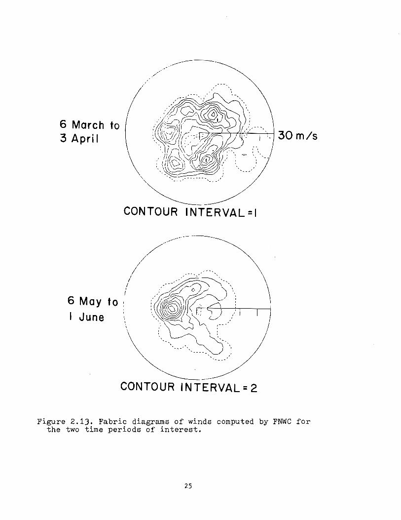
2.13 Fabric diagrams of winds computed by FNWC forthe two time periods of interest. 25

2.14 (a) Wind fabric diagrams for 6 March to 3 Aprilfor coastal stations at Pt. Riu and Pt. Manby. 26

2.14 (b) Wind fabric diagrams for 6 March to 3 Aprilfor buoys EB43 and EB70. 27

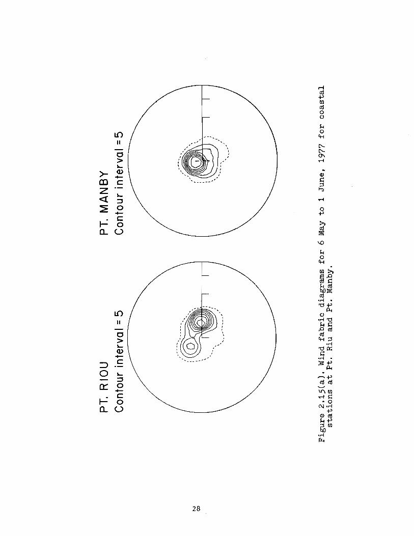
2.15 (a) Wind fabric diagrams for 6 May to 1 June,1977 for coastal stations at Pt. Riu andPt. Manby. 28

2.15 (b) Wind fabric diagrams for 6 May to 1 June,1977 for buoys EB43 and EB70. 29

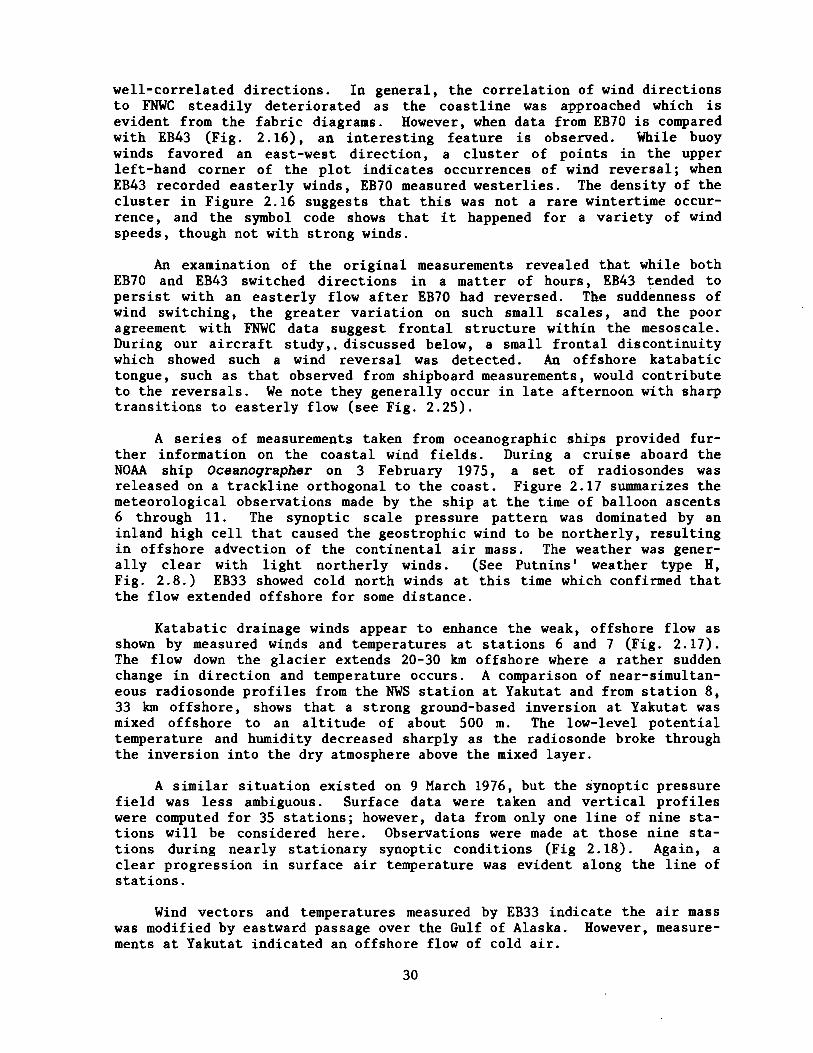
2.16 (a) Correlation plot of wind direction compar-ing winds at EB43 and EB70 for the period of6 March to 3 April, 1977. 31

2.16 (b) Same as 2.16(a) for the period of 6 May to1 June, 1977. 32

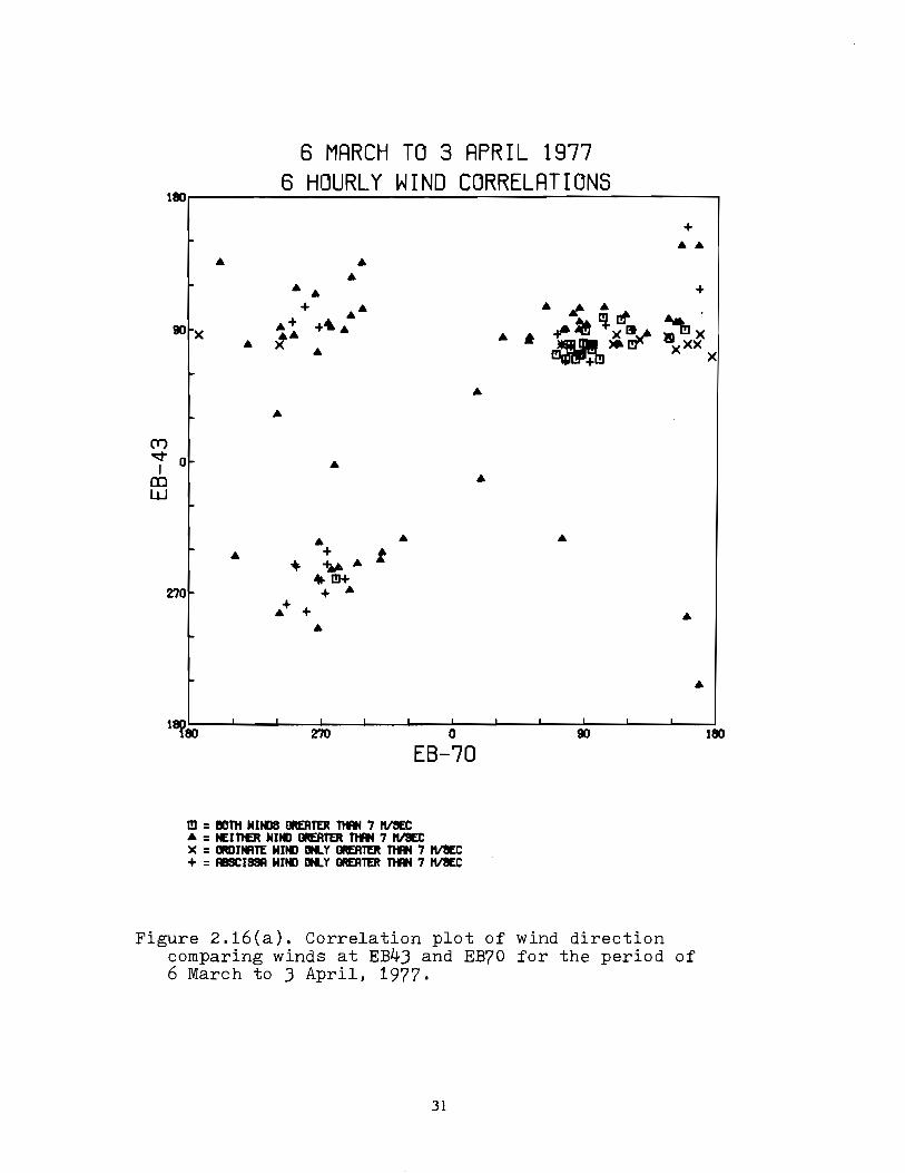
2.17 Observations of wind and temperature for the3 February 1975 trackline. The vertical profilesof potential temperature and mixing ratio at sta­tion 8 agree well with the Yakutat profile whichoccurred at the same time. 33

2.18 (a) Weather map for the Gulf of Alaska-1200 GMT,9 March 1976. Temperature and dewpoint are in F.(b) Surface observations for the 9 March 1976trackline. Open circles indicate clear skies;temperature (OC), coded pressure (mb) , and dew­point temperature (OC) are shown in clockwiseorder beginning from a point roughly NW on thesymbol. 34

2.19 Contour plot of (a) potential temperature and(b) mixing ratio as a function of distance off­shore. Of note are the katabatic cold wedge andcold core at 1000 m. 36

2.20 Profiles of temperature and winds from radio-sonde (x), tethered balloon ascent (solid line),and descent (dotted line) taken at station 6, about6 km offshore. Wind direction indicates a sharptransition at 250 m. There is evidence of ashallow mixed layer at 30 m. 37

v

2.21 Weather during the Queen Air flight on 25 Feb­ruary 1977. The upper map is the 12Z, 500 mbchart and the lower map is the 18 Z, surfacechart. Observed winds are plotted on the maps. 39

2.22 Satellite photo of the Gulf of Alaska on 25 Feb-ruary 1977. 40

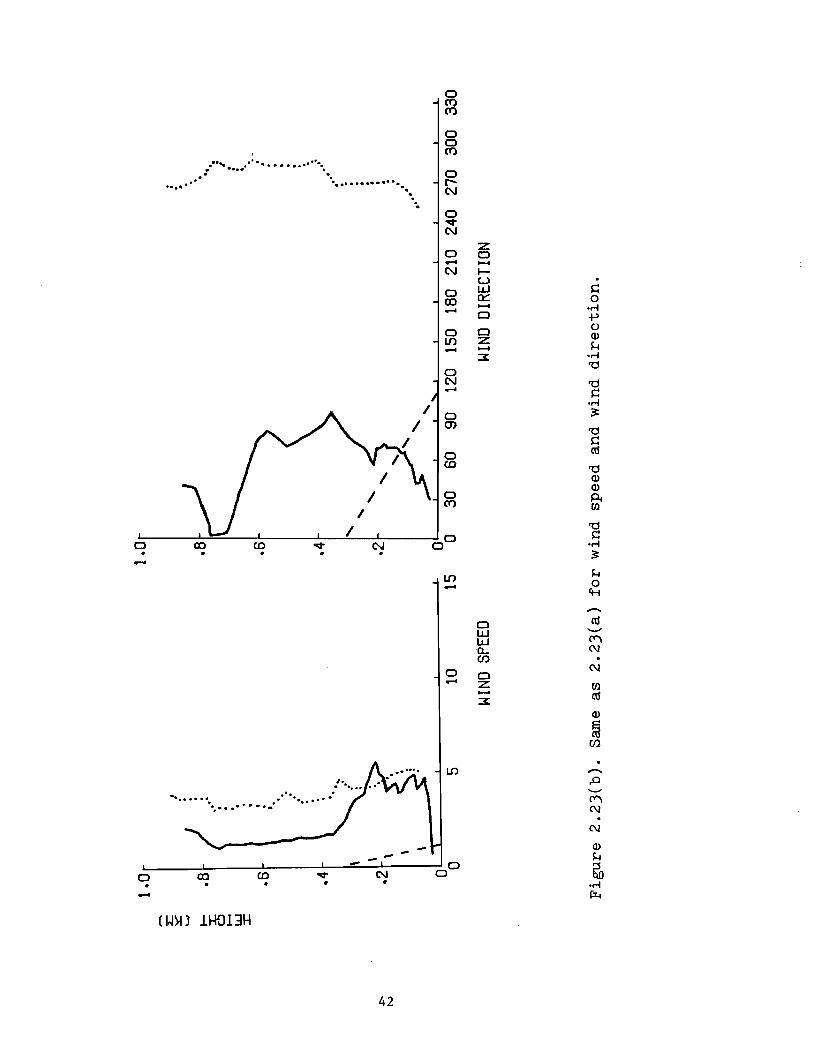
2.23 (a) Vertical profiles of potential temperatureand mixing ratio taken by the Queen Air duringthe flight. The solid line is at the inshorepoint, in the vicinity of stations 6-8. Thedotted line is offshore, station 9. The dashedline is a sounding taken at Yakutat NWS at thesame time. 41(b) Same as 2.23(a) for wind speed and winddirection. 42

2.24 (a) Distribution of wind speed and direc-tion along the offshore trackline. Data isinstantaneous from an altitude of 30 m. 43

2.24 (b) Distribution of temperature and mixing ratioalong the offshore trackline. Data is instantan­eous from an altitude of 30 m. The dashed lineis sea surface temperature as inferred frominfra-red radiation. 44

2.25 Winds measured during the Queen Air flight.The data are from an altitude of 60 m and arehorizontal averages over about 11 km. 46

3.1 Example of flow conditions at the MalaspinaGlacier which could lead to the observed windsand temperature anomalies at the data buoys. 47

Tables

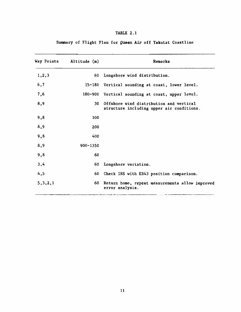
2.1 Summary of Flight Plan for Queen Air off YakutatCoastline

vi

11

Observations of South Alaskan Coastal Winds

by

R. M. Reynolds, S. A. Macklin, and T. R. Hiester 1

Pacific Marine Environmental LaboratorySeattle, Washington 98105

lBatelle LaboratoryRichland, Washington 99352

ABSTRACT. Two main groups of offshore katabatic flow, fall windsand gravity winds, are defined and discussed. Climatologicalaverages of the Alaskan synoptic weather network define thoseweather patterns that promote offshore flow on the south Alaskancoast.

Observations were taken over several years near the MalaspinaGlacier on the south coast of Alaska using research ships, buoys,and on one occasion an instrumented aircraft. At the beach, windsblow offshore almost continuously in the winter, and at night inthe summer. Their direction is seemingly unperturbed by synopticvariations. Within approximately 50 km of the beach, the wind isunpredictable by synoptic analysis. Upper-air soundings in thisregion reveal a complicated process whereby coastal air flowsunder the marine boundary layer and subsequently is absorbed intoit by a process of entrainment and warming.

1. INTRODUCTION

This paper discusses offshore coastal winds and their transition to theoceanic regime. Land breezes are ubiquitous features of high-latitude moun­tainous coastlines, occurring on a variety of spatial and temporal scales.There is a dearth of observation concerning these flows and their transi­tion, and indeed, some confusion as to their terminology.

We present in the sections to follow a general discussion of coastalwind types and the factors which serve to modify them offshore. An exten­sive set of observations which define the salient aspects of katabatic flowsand their modification is presented and discussed.

1.1. Survey of Coastal Wind Types

Katabatic flow can be subdivided into two main groups, fall winds andgravity winds (Huschke, 1959). Both are driven by pressure force; thedifference being one of scale.

Fall winds are large-scale phenomena, often driven by large-scalepressure gradients and requiring a reservoir of cold air from an elevatedinterior. The air is initially cold enough that it remains relatively cold

despite adiabatic warming during descent. A well-known example of a fallwind is the bora (from the Greek ~vpeaa, meaning N-wind) which occurs on theAdriatic coast. Other locally named fall winds of some importance are theMistral in southern France, the Athos in Greece, and the oroshi of Japan(Yoshino, 1975). As fall winds are driven by synoptic pressure patterns,they tend to appear suddenly, last for a few days, and then fade much moreslowly than their onset. Temperatures drop by several degrees, and relativehumidity often drops below 10% (ibid.). The outstanding characteristic ofthe bora is its gustiness and violent winds. As the cold air flows down tothe sea, it accelerates and becomes highly turbulent (Defant, 1960).

Kilday (1970) has performed a study to determine the conditions favor­able for the occurrence of bora winds in southeast Alaska (called Takuwinds). It is possible to extend his arguments to other areas along theGulf of Alaska coast. Fall winds occur where the terrain drops sharply andwhere there are mountain ranges near and parallel to the coast. If a verycold air mass passes over a mountain barrier, or if under the right pressureconditions, deeply chilled continental air is forced across the mountainranges, the cold air cascades down the steep slopes to the warm coast.Observations indicate that the time of onset of wind is independent of adiurnal effect and maximum velocities can occur at any time of the day.

Fall winds can be classified as either cyclonic or anticyclonic depend­ing on the overall synoptic pattern which might exist. In either case,isobars along the coast are tightly packed and winds blow predominantlyacross isobars and offshore (Fig. 1.1). The anticyclonic type producesstrong, gusty winds with calm periods in between. The weather remains clearand dry. The cyclonic type is characterized by cloudy skies, snow, and onlymoderately cold temperatures. The same classifications and features areobserved in the bora and mistral (Yoshino, 1975, p. 361).

Often large land/sea temperature differences are sufficient to producenear-continuous offshore flow. A cold continental air mass biases theinterior pressure higher than the warmer ocean regions, equivalent to ananticyclonic fall wind. Often, these winds drain large river valleys suchas the Susitna in southern Alaska. In this case, the drainage winds arechanneled down Cook Inlet and dominate the winter wind field as far south asAugustine Island (Macklin et al., 1980). When that bias is accentuated byan approaching oceanic cyclone, the drainage winds can become quite intense.

The gravity wind is a much more local katabatic flow. Often calleddrainage wind, mountain wind, or katabatic wind interchangeably, it iscaused by greater air density near the slope than that of the same levelaway from the slope. Highly dependent on net radiation at the surface, theair flows downhill in balance with frictional drag, the Earth's coriolisforce, and the impressed synoptic scale pressure field. Because of rota­tion, the flow is inclined away from the line of steepest descent (Ball,1960), but is still focused into valleys and estuaries where violent windscan occur. A particular type of drainage wind is the glacier wind, a con­tinuous downdraft along the surface of the glacier which is relativelyindependent of insolation (Defant, 1960). Its thermal gradient is due tothe temperature difference between the ice surface and the free air at thesame altitude. In general, these winds are relatively light, but there aredramatic exceptions.

2

200km

Figure 1.1. Satellite photograph of the Gulf ofAlaska showing offshore winds and modificationinto the synoptic scale pattern.

3

A mountain wind is an even more localized katabatic flow which occurson mountain sides, blowing down the flanks of the valleys and then down thevalley axis (Defant, 1960; Yoshino, 1975).

Virtually every estuary on mountainous, high-latitude coastlines willbe dominated by an axial outflow resulting from katabatic drainage. Oftenthe winds at the mouths of estuaries such as Icy Bay on the coast of Alaska

exhibit 50 ms -1 winds or greater (Searby, 1969). When the estuary is theterminus of one or more glaciers, the outflow winds are relatively persis­tent, especially in the winter months, showing little diurnal variation.Estuaries without glaciers exhibit much more diurnal katabatic winds, callednocturnal winds (Yoshino, 1975, p. 408). The cold air masses gathered onthe upper slopes make up the first motion of the overall flow; they becomethe mountain wind in the valleys; and finally they are called land breeze onthe coastal plain.

At the coast, an offshore wind often flows under the prevailing marineboundary layer. In the case of an existing land/sea breeze circulation itwill underflow the larger circulation. A land breeze will be strengthenedin this way (Yoshino, 1975, p. 160).

1.2 Offshore Modification of Coastal Winds

The offshore winds which have been discussed do not persist very farout to sea. The bora is seldom seen beyond 60 km (ibid., p. 366). Simi­larly, the Taku winds of southeast Alaska quickly merge into the open-oceanwind field. Figure 1.1 indicates a typical distance of 70 km for cross­isobaric fall winds to turn into a balanced open-ocean direction.

Surface friction alone cannot bring the winds into offshore palance inanything near the observed distances. Mahrt (1974) modeled the response ofa layer-averaged neutral boundary layer flow to specified, time-dependent,

pressure gradients, and found a frictional damping time (e-1 time scale)given by

(1.1)

where h is the layer height, CD the drag coefficient, [V] a scale velocity

(necessary for a linearized drag formulation), " is the angle between thelayer-mean wind vector and the surface stress vector, and wE is the enter-

-3 -1tainment rate. Typically, over the ocean CD = 1.5 x 10 , [V] = 5 ms ,

h = 1 km, and both" and ~~ are small. In this case, T =1\ days; with an

advection velocity of 5 ms ,this corresponds to an adjustment distance ofover 600 km.

However, for fall winds and gravity winds, the situation is much dif­ferent. In the case of fall winds, the inversion base is lower; typically

~ -1h ~ 200 m, and [V] = 20 ms . Entrainment is greatly enhanced; the coldair over a warm ocean generates buoyant thermals, which penetrate the inver­sion base. Surface-layer turbulence and shear-induced turbulence at theinversion base both contribute to the entrainment rate. It is likely there-

4

,., -1fore to have wE ,., 0.1 ms which leads to adjustment times of ~ hr which

corresponds to 30 km.

Gravity flows are generally much shallower, but the velocity is lessalso. Additionally, there is pronounced growth in h offshore. Mahrt'sformulation does not apply to rapidly growing mixed layers, but an heuristicargument, based on equation (1.1) can be advanced. In his dissertationReynolds (1980) shows that as the boundary layer becomes shallower, wE

becomes a strong function of h- 1 . Therefore, equation (1) suggests thatadjustment becomes weakly dependent on h.

When the synoptic pressure pattern directs a continental air mass off­shore, the process of boundary layer growth and warming occurs on a muchlarger scale. Generally called air modification, it provides an importantmechanism for the poleward flux of heat in the global energy balance, espe­cially in the 40-50° latitude zone. One of the early analytical models ofthe boundary layer growth was an integrated, mixed-layer model by Businger(1954; 1972).

2. MEASUREMENTS OF COASTAL WINDS IN ALASKA

The research for this report is based on a collection of observationsof coastal winds along the coast of Alaska. The measurements given herehave been taken by the authors since 1975 and continue at this time.

Most of the measurements presented here were made in the vicinity ofthe Malaspina Glacier, a broad semicircular glacier on the coastal side ofthe dramatic St. Elias Mountains (Figs. 2.1 and 2.2). A vast entanglementof glaciers and snowfields in these mountains provides a source area forfall winds. As the air descends toward the coast, it is focused into IcyBay and Yakutat Bay where winds are often observed by fishermen and weatherobservers (Searby, 1969).

2.1 Instruments and Analysis

Initial observation sets were simply standard ships I meteorologicalmeasurements of temperature, humidity (wet-bulb temperature), wind speed anddirection, and some gross observations of sea state and clouds. The accu­racy of ships' measurements have been discussed by Ching (1974) and Godshallet al. (1976). Wet- and dry-bulb temperatures were measured hourly atbridge height, 18.2 m above the ocean surface. During intercomparisons withother vessels and buoys during the GARP Atlantic Tropical Experiment (GATE),bridge temperatures were found accurate to O. 7°C. Winds were measured atmast height, 36 m. During the same GATE intercomparisons, these were shown

-1to be accurate to approximately 1 ms . It is understood that the aboveintercomparisons were made under optimum conditions; during routine opera­tions, with the ship underway, the results are much poorer. It mustcontinually be borne in mind that a sequence of ship observations is notconcurrent, and can be treated as such only with care. Diurnal and synopticscale processes can seriously contaminate the observed data.

5

10I

I~O km. +

.14070

20 N.MI.I

i2~o

oI+

eFNWC

Figure 2.1 A Lambert conformal projection of the Malaspina Glacier showingelevations in feet. Shaded areas suggest the limit of the glacier.

Figure 2.2 An isometric picture of the topography set on a 5-km grid.

6

From 1974 to 1977, during four cruises to the region, upper air datawere collected with standard National Weather Service (NWS) radiosondes.The NWS radiosondes, older 403 MHz units, cycled between temperature, rela­tive humidity, and reference channels in response to ambient pressurechanges. Designed to profile the entire atmosphere, a pressure-actuatedswitching mechanism allowed only a few samples of the boundary layer, andthe boundary layer and inversion base generally appeared as a confuseddecrease in temperature. Therefore, we needed to analyze our radiosondecharts to a much finer detail than is nomally provided by NWS. We digi­tized as many points during a switch closure as possible in hopes of betterresolving the lower profiles.

After 1977 a much more sophisticated 'airsonde' system provided greaterdetail of the lower troposphere. The airsonde makes over 50 samples throughthe boundary layer. A product of AIRCO, Inc., the sonde is a small wingedstyrofoam package weighing considerably less than the standard radiosonde.It has a pressure sensor and wet-/dry-bulb thermistors which are aspiratedas the body spins on its tether during ascent. The themistors are accurateto O.l°C, and the pressure sensor to 1 mb. These errors result in approxi-

mately 2% relative humidity uncertainty, or 2 x 104 in mixing ratio, andabout 7 m height uncertainty. Neither of the above sounding systems has thecapability of measuring winds aloft. Generally, conditions on the ship wereunfavorable for performing the sensitive pibal measurements needed to deducewinds from the balloon trajectory.

On one occasion (see Fig. 2.20), a boundary layer profiler, supportedby a kytoon, made detailed measurements of air temperature, wet-bulbtemperature, wind speed, wind direction, and pressure. The pressure sensormalfunctioned, but reasonable height estimates were made in the followingway: ascent and descent were scaled by matching heights at which sharptransitions in wind direction occurred and by assuming constant rates ofascent and descent; a radiosonde profile, taken just prior to kytoon launch,established an absolute height scale.

To ascertain the effects of the coastal mountain range on the offshorewind field, the authors analyzed data from several closely spaced meteoro­logical stations (Fig. 2.3), including three National Data Buoy Office(NDBO) buoys. EB33 was placed at 58°30'N, 141°00'W, near the MalaspinaGlacier. It had a boat-shaped (nomad style) hull (length =6 m, beam = 3 m,depth = 2.5 m) and the sensors were approximately 5 m above the surface.From October 1974 to September 1976, it operated sporadically during thewinters, but was reasonably reliable in the less stormy summers. The loca­tion of this buoy, about 150 km offshore, probably placed it beyond anynear-coastal influences.

In the fall of 1976, the NDBO installed two buoys in the same vicinity,but much closer to shore. EB70 was deployed at 59°30'N, 1400 12'W, approx­imately 60 km offshore. It was a 12 m discus hull buoy with all sensorslocated 10 m above the ocean surface. EB43 was a nomad hull similar toEB33, and was placed at 59°48'N, 142°00'W, only about 20 km offshore. Thesebuoys operated from September 1976 to October 1977, but unfortunately,during the interesting months, November-January, EB43 was out of order.

The NDBO received all data by high frequency (HF) and satellite (GOES)transmissions. After editing the data they reduced it to standard archival

7

Mo

un

tS

t.E

lia

s ·18

00

8.1

40

70

EB

43

e

eF

NW

C

o10

20

N.M

i.I

II

II

o2

55

0km

.+8

84

80

~

eE

B7

0

00

Fig

ure

2.J

.Sa

me

map

as

Fig

ure

2.1

.sh

ow

ing

po

siti

on

so

fm

ete

oro

log

ical

stati

on

su

sed

inth

isst

ud

y.

format in which wind speed is given to the nearest mph and direction to thenearest 10°. The buoys averaged wind speed, direction, and air and seatemperatures over an 8-minute period and reported every 3 hours.

During the spring and summer of 1977, we measured coastal winds at tworemote sites. Point Riou (59°55'N, 141°32'W) is at the mouth of Icy Bay andPoint Hanby (59°41'N, 1400 17'W) is at the mouth of Yakutat Bay (Fig. 2.3).The stations, manufactured by Climatronics, Inc., recorded wind speed, winddirection, and air temperature on a 30-day strip chart with about the sameaccuracy as the data buoys.

At the Yakutat airport, a NWS facility provided hourly surface observa­tions and twice-daily upper air soundings. The U.S. Navy's Fleet NumericalWeather Central (FNWC) provided surface winds from a synoptic scale pressureanalysis. FNWC computes this analysis for their polar stereographic model,which has a mesh length of 481 km at 60 0 N. A geostrophic wind was deter­mined (Bakun, 1973) by a computation of pressure gradient using as-pointarray centered at 59°39.9'N, 142°10.5'W (Fig. 2.3). They then approximatedthe surface wind by reducing the geostrophic wind by 30% and rotating itleft by 15°.

Their analysis results from a blending of fields derived from pastmodel runs, previous analysis extrapolated forward, and all current measure­ments of winds and pressure. The buoys are part of this set, and thereforeFNWC-derived winds are not independent of them. However, after blending andsmoothing the field on a synoptic scale we do not expect to see pronouncedlocal effects in these winds.

From 21 February to 3 March, 1977, we flew tracklines off the MalaspinaGlacier with an instrumented aircraft, the Queen Air (Fig. 2.4) (operated bythe National Center for Atmospheric Research, (NCAR), Boulder, Colorado).Previous shipboard measurements were handicapped by the time necessary for aship to move between stations. Temporal atmospheric processes interferedwith the interpretation of the spatial atmospheric variations.

Possessing high quality instrumentation, a high-speed data logger, anda precision inertial navigational system (INS), the Queen Air could collectdata sufficient to describe the turbulent behavior of the boundary layer(Lenschow, 1972). The three-dimensional wind field, temperature, humidity,and sea surface temperature are among the many measured parameters. At an

airspeed of 250 km hr-1, the Queen Air easily covered the Yakutat-Icy Bayarea in 3\ hours. A typical flight plan is shown in Figure 2.5 and issummarized in Table 2.1.

Before undertaking any computations from flight data gathered duringthis period, we made a thorough appraisal of the quality of time seriesplots. All bad data could be avoided entirely by judiciously selectingcontinuous intervals of level flight and uniform heading from the timeseries for further processing. Because of drift in the aircraft's INS, the

absolute wind speed is typically known only to within 2 ms- 1 and wind direc­tion to within 10°. Since the magnitude of these errors is time-dependentwith a period of 84 minutes (Lens chow , 1972), relative differences betweenadjacent measurements are no more than 0.3 mls over a 10 km averaging dis­tance.

9

Figure 2.4. The research aircraft operated by the NationalCenter for Atmospheric Research. The Queen Air isinstrumented for low level turbulence measurements.

60·

59·

142·

o 20 40, ! I I I

KILOMETERS

0- AIRCRAFT WAY POINTSLONGSHORE LEGS AT 60 MOFFSHORE LEGS AT 30. 60, 10 •200,400 MAND SLANT LEGS FROM900-1400 M'

142 0

140·

Figure 2.5. Typical flight plan for the Queen Air.

10

TABLE 2.1

Summary of Flight Plan for Queen Air off Yakutat Coastline

Way Points

1,2,3

6,7

7,6

8,9

9,8

8,9

9,8

8,9

9,8

3,4

4,5

5,3,2,1

Altitude em) Remarks

60 Longshore wind distribution.

15-180 Vertical sounding at coast, lower level.

180-900 Vertical sounding at coast, upper level.

30 Offshore wind distribution and verticalstructure including upper air conditions.

100

200

400

900-1350

60

60 Longshore variation.

60 Check INS with EB43 position comparison.

60 Return home, repeat measurements allow improvederror analysis.

11

A standard time series analysis package, developed as a general tool,produced useful graphics for all the time series shown here. Aside fromroutine plots of speed, direction, temperature, etc., which need no expla­nation, a most useful graphic was the fabric diagram in various forms. Thename fabric diagram is borrowed from a similar graphic developed by Davisand Ekern (1917). An example of the four forms of the plot is given inFigure 2.6.

A brief summary of the construction of the fabric diagram follows: A41 x 41 grid of possible u,v wind vector components defines 40 x 40 boxes ona space where the polar radius is proportional to the square root of thewind speed, r «~s. All the data to be analyzed are sorted according to thewind vector, and the cumulative amount of a chosen quantity--number ofoccurrences, wind stress, heat flux, temperature variance--is calculated foreach box of the grid. Finally, a 5 x 5 top-hat, smoothing kernel (not abox-car) is run over the grid to effect a reasonable picture. The grid iscontoured with a simple linear interpolation routine. Contours represent 1%of the total accumulation per 1% area of the enclosed circle. Wind direc­tion is plotted according to meteorological convention, the true compassdirection from which the wind is blowing. By plotting wind speed as thesquare of the radius, equal areas of contours represent equal percentages,thus compensating for the spreading of radial line segments.

The frequency fabric diagram (~ig. 2.6) is basically a contour map ofthe wind velocity probability distribution. The probability of windsoccurring in any velocity range are calculable from this diagram. Thewind stress or energy fabric diagram is a contour of the % total energy(expressed as a square of the wind speed) per 1% area of the circle. Whilethis plot is often similar to the frequency diagram, it occasionally pointsout highly preferred directions for the stress. As the ocean responds towind stress and not frequency, this plot is valuable to the physical ocean­ographer.

Fabric diagrams are applied to the observed temperature in two ways.If surface temperature is available, then the heat flux fabric diagram isestimated by H = U(e f - 8 . ) [CDP] for each box. If 8 f is not avail-o s c al.r s cable, then the average e. over the record may be substituted for 8 f .al.r s cAnother useful variation is to calculate the temperature perturbation 68 =(e - 8) for each box. The resulting temperature Rerturbation fabric diasrampoints out preferred winds which accompany warmer or colder air. Figure 2.6points out a sharply defined range of wind speeds and directions whichadvect colder air to the site. This will be discussed in greater detail inSection 2.3. Finally, the temperature variance fabric diagram points outregions which contribute to the variance of the series.

2.2 Weather Patterns Over the South Alaskan Coast

The Gulf of Alaska is a region of extremely changeable sea-level pres­sure. Two winter features of the monthly mean barometric pressure field(Fig. 2.7) are the Aleutian Low, which dominates the North Pacific, and theContinental High which covers the main land masses of Siberia, Alaska, andBritish Columbia. In summer, increased heating over land produces a rela­tively low-pressure continental region which weakens the Aleutian Low; in

12

Fre

qu

ency

Fab

ric

Dia

gra

mC

onto

urin

terv

al=3

No.

po

ints

=111

Ene

rgy

Fa

bri

cD

iag

ram

Con

tour

Inte

rval

=4

Avg

.en

erg

y=

43

m2s

-2

","

-.....

.,",'

I

"0

'I

II

I\

,\

,\

,,

I

'....-

"

'-....,-.

....

-

(@'O

-'/'I;;

\(~

I'<

I\ ,

, '....

_J

-",,_

\--

\ \"

'--

......

Lv

Fig

ure

2.6

(a).

Ty

pic

alfa

bri

cd

iag

ram

so

fw

ind

freq

uen

cyan

den

erg

y.

The

data

isfr

om

EB43

for

the

peri

od

of

6M

arch

to3

Ap

ril,

19

77

.

..­ -l:'-

Te

mp

era

ture

Pe

rtu

ba

tio

nF

ab

ric

Co

nto

ur

inte

rva

l=

ID

iag

ram

(5J o

Te

mp

era

ture

Va

ria

nc

eF

ab

ric

Dia

gra

m

Co

nto

ur

inte

rva

l=3

Va

ria

nc

e=

.62

°K

2

Fig

ure

2.6

(b).

Fab

ric

dia

gra

ms

of

tem

pera

ture

pert

ub

ati

on

and

vari

an

ce

for

the

sam

ed

ata

as2

.6(a

).

SEPTEP7I3EI('

Figure 2.7. Average meteorological conditions in the Gulf ofAlaska for various months of the year. Solid arrows are principalstorm tracks, dashed arrows are secondary tracks. (From Searby,1969)

15

winter excess terrestrial cooling produces the Continental High and ampli­fies the Aleutian Low. The trough of the Aleutian Low controls the passageof an endless stream of cyclonic disturbances traveling eastward across theNorth Pacific. Figure 2.7 shows average storm tracks for various times ofthe year wherein the effect of the Aleutian Low is evident.

Mean pressure fields bear little resemblance to the actual distributionat any time. In an attempt to treat statistically the daily weather pat­terns for the Alaskan region, Putnins (1966) analyzed over 18 years of sur­face and 500-mb weather maps. After developing a classification schemewhich described 22 synoptic patterns, he determined the frequency of thesepatterns for each month of the year. Figures 2.8 (a-d) are a sample of hisresults, the six most common weather types for 4 months, representing eachseason. The figures are real maps selected as typical for the classifica­tion type. The nature of the main barometric features of the pressure fieldis apparent in these maps, especially the Aleutian Low. The convergence ofcyclonic disturbances into the Gulf of Alaska is also apparent. Observedwinds are reported with the following convention: indicators point in thedirection from which the wind is blowing, one full barb represents a speed

of 5 ms- 1, one-half barb indicates 2.4 ms- 1 , and no barb implies wind speed

less than 1.24 ms- 1/2.

The coastal mountains of British Columbia and Alaska present a barrierto the movement of disturbances with the result that many of them stagnatein the Gulf of Alaska for several days, especially if there is inland highpressure. Occasionally, if unable to move forward, these cyclones take aretrograde course toward the northwest. As Bilello noted in 1974, once astorm has moved against the mountain ranges bordering the northern Gulf ofAlaska, only a vigorous circulation aloft can cause it to move further.With moderate southerly winds, maritime air moves into the coastal valleysand the front then has a tendency to become stationary along the AlaskaRange. Strong southwesterly winds, however, occasionally force the frontfurther up the valleys. At this point there is no definite physical barrierto impede movement of the front so it can now readily penetrate to theinterior of the state and influence the weather accordingly. Nevertheless,exactly how far inland the front moves is dependent almost entirely upon thestrength and persistence of the steering level winds. As marine air crossesthe Alaska Range, a great deal of orographically induced precipitationoccurs. For example, Middleton Island (150 km south of the coast) has1.47 m of annual rainfall while there is a prodigious precipitation measuredat coastal stations such as Cape St. Elias and Yakutat (3.36 m).

Based on the criterion for a fall wind condition as outlined in Section1.1, patterns such a A, AI' or D are appropriate to drive a fall wind from

the high snow plateaus of the St. Elias Mountains. The frequency of occur­rence of these patterns--marked in the upper right-hand corner of eachpattern--varies from about 5% in the summer to 40% in the winter.

2.3 Observations at the Malaspina Glacier

During late 1974 and 1975, EB33 made wind measurements 150 km off­shore of the Malaspina Glacier. When compared to winds computed from theglobal model of FNWC a slight preference for a bimodal wind field appears

16

(0) FEBRUARY

(b) NOVEMBER

Figure 2.8(a)(b).~1ost common synoptic scale types as classified byPutnins (1966). Classification symbol and percentage of occuranceare shown in the upper right hand corners.

17

(c) MAY

(d) AUGUST

Figure 2.8(c)(d).r~ost common synoptic scale types as classifiedby Putnins (1966). Classification symbol and percentage of occuranceare shown in the upper right corners.

18

(Fig. 2.9). In the winter of 1974/75 there were many occurrences of coldair outbreaks; the air would be up to 10° colder than the sea surface atthis place for four days to a week duration. In spite of a fairly broaddistribution of wind directions, the winds from the east, particularly theNE or ENE carried the coldest air (Fig. 2.10). It will be shown later thatthis is in keeping with the notion of large-scale air modification, wherethe isobars offshore are roughly perpendicular to the coastline. Such wouldbe the case for pattern H or Al in Figure 2.8 if the low center were dis-

placed to the east. That is, the continental air mass which falls offshorealigns with the isobars of a low-pressure disturbance and produces coldeasterlies at the buoy (Fig. 2.11).

The NDBO installed buoys EB43 and EB70 in late 1976 and they operatedsporadically throughout 1977. They were located much closer to shore thanEB33 (10 and 60 km respectively), and hence we hoped to see a strongercoastal influence. The remote coastal stations at Point Riou and PointManby operated reasonably well during their stay; they failed only as aresult of occasional bear maulings. All stations operated well during twotime periods: 6 March to 3 April and 6 June to 6 July.

The FNWC-derived surface winds for these time periods show a broadrange of directions (Figs. 2.12, 2.13). Wind directions exhibited a coun­terclockwise rotation indicative of the passage of cyclonic disturbances tothe south. The more frequent westerly winds in the May diagram result froma stagnant system which occurred during the first part of the period. Datafrom a single month are insufficient to assess whether such prolonged windswere typical.

Data buoys and land stations recorded wind events which appeared on theFNWC record. The land stations showed the events with a much reduced windspeed while the buoys showed only a slight reduction in wind speed from EB70to EB43 (which was positioned closer to shore). The wind speed of FNWCinexplicably agrees more closely with EB43. Overall, wind speed correlationcoefficients between the data buoys and FNWC are from 0.70 to 0.85.

Wind fabric diagrams (Figs 2.14, 2.15) show that winds at the four sta­tions are different. The FNWC winds exhibit no special preference fordirection while all the measured winds showed distinct influence of thecoastline. EB70 had an almost symmetrical bimodal character with the mostcommon wind directions approximately 115° and 270°. EB43 data showed bimo­dality also, but during March the winds from the east were more common(probably an offshore manifestation of the winter drainage winds fromMalaspina Glacier). During summer, winds at EB43 were more common from thewest, and the two buoys were better correlated. Coastal winds measured atPoint Riou and Point Manby showed definite orographic influence. Duringwinter at Point Riou, the combined katabatic drainage winds and mountainblockage resulted in winds that blew almost continuously from the northeast,down the glacier. In addition to orographic influence, diurnal forcing wasapparent during both March and May. During the coldest period of the day,northerly drainage flow from the glacier dominated; in the daylight hoursthe flow was more often from the northeast and east.

We extracted additional details of the flow distribution by the use ofcorrelation plots in which wind directions from two different records wereplotted on the same graph. Points clustering about a 45° line represent

19

CONTOUR INTERVAL =I

CONTOUR INTERVAL=I

Dec. 1974

Feb. 1975

CONTOUR INTERVAL=3

CONTOUR INTERVAL=2

Figure 2.9(a). Fabric diagrams of wind observations atEB33 compared with those computed by FNWC. The circlerepresents a 30 ms- 1 wind and ticks mark 10 and 20 ms-1speed.

20

\

............

....'~

jI\--~;;)

\~\>-'(.: ..'. C>. ,

. -. ......., .'

Aug. 1975

CONTOURINTERVAL=2

CONTOUR INTERVAL = I

Oct, 1975

CONTOUR INTERVAL=2

...-(.)(; Q \ •.•;,

"'" '-----'" ~,

CONTOURINTERVAL=2

Figure 2.9(b). Fabric diagrams of wind observations atEBJJ (left side) compared with those computed byFNWC.

21

CONTOUR INTERVAL=4

7"I.T-f--r--i 8/ 75u=OA

CONTOUR INTERVAL =2

12/74 :u=2.7

CONTOUR INTERVAL=2

r=:--~'ftr--110/75

u= 1.7

/.~/ ::.::::::: ::: .....

............ ,

CONTOUR rNTERVAL=2

2/75u=2.0

Figure 2.10. Temperature perturbation fabric diagrams forfour months for EBJJ, 150 km offshore of MalaspinaGlacier, AK. The variance of temperature is shown eachmonth.

22

Figure 2.11. Schematic of a typical wind field on the Alaskancoast in which EB33 registers cold air.

23

FNWC 6 MRR THROUGH 3 RPR 19773Or-__T.:.....:I:..;...:M:.=.E--=S:.::E:.;..:R.:...:IE:..:S:......:::.:DF_..:::.6......:.H.:.:::D:.:::U~RL~Y~OR~T~R __---.

24

ita!t2~ I,.

B .

0

\80

270

\800 \ 2 3 4 5 a 7 8 8 \0 \I \2 \3 \4 \5 \8 \7 \a \8202\ 22 23 24 25 21 27 21 28 30 3\OAYS WTEJt OOZ IF f1RllT OAY IF BlEIl

FNWc 6 MRY THROUGH 1 JUN 19773Or-__T:....::1..:...;,M=.E--=S:..=:E.:..:..R:..:IE:;:S_O:::..:.F_:::::....6....:..H:.:::O~UR~L:....:..Y......:O~R~T~R __----.

Figure 2.12. Time series of wind speed and direction as com­puted by FNWC for the two time periods of interest.

24

6 March to3 April

----------

/

CONTOUR INTERVAL =1

30m/s

Figure 2.1]. Fabric diagrams of winds computed by FNWC forthe two time periods of interest.

25

PT

.RIQ

UC

onto

urin

terv

al=

5

PT.

MA

NB

YC

onto

urin

terv

al=

4

N 0'

":

.,

'"--

...."

~-'

Fig

ure

2.1

4(a

).W

ind

fab

ric

dia

gra

ms

for

6M

arch

toJ

Ap

ril

for

co

ast

al

stati

on

sat

Pt.

Riu

and

Pt.

Man

by.

EB

43

Con

tour

inte

rval

=3

~

EB

70

Con

tour

inte

rva

I=2

N -...J

-""

..'

:/"@

Jo/'~u~

'-:I

:I(

".....

.~

Fig

ure

2.1

4(b

).W

ind

fab

ric

dia

gra

ms

for

6M

arch

to3

Ap

ril

for

bu

oy

sE

B43

and

EB

70.

PT.

RIO

UC

onto

urin

terv

aI=

5P

T.M

AN

BY

Con

tour

inte

rval

=5

N 00

Fig

ure

2.1

S(a

).W

ind

fab

ric

dia

gra

ms

for

6M

ayto

1Ju

ne,

1977

for

co

ast

al

stati

on

sat

Pt.

Riu

and

Pt.

Man

by.

EB

43

Con

tour

inte

rval

=3

EB

70

Con

tour

inte

rval

=2

N \0

~

Fig

ure

2.1

5(b

).W

ind

fab

ric

dia

gra

ms

for

6M

ayto

1Ju

ne,

1977

for

bu

oy

sE

B4]

and

EB

70.

well-correlated directions. In general, the correlation of wind directionsto FNWC steadily deteriorated as the coastline was approached which isevident from the fabric diagrams. However, when data from EB70 is comparedwith EB43 (Fig. 2.16), an interesting feature is observed. While buoywinds favored an east-west direction, a cluster of points in the upperleft-hand corner of the plot indicates occurrences of wind reversal; whenEB43 recorded easterly winds, EB70 measured westerlies. The density of thecluster in Figure 2.16 suggests that this was not a rare wintertime occur­rence, and the symbol code shows that it happened for a variety of windspeeds, though not with strong winds.

An examination of the original measurements revealed that while bothEB70 and EB43 switched directions in a matter of hours, EB43 tended topersist with an easterly flow after EB70 had reversed. The suddenness ofwind switching, the greater variation on such small scales, and the pooragreement with FNWC data suggest frontal structure within the mesoscale.During our aircraft study,. discussed below, a small frontal discontinuitywhich showed such a wind reversal was detected. An offshore katabatictongue, such as that observed from shipboard measurements, would contributeto the reversals. We note they generally occur in late afternoon with sharptransitions to easterly flow (see Fig. 2.25).

A series of measurements taken from oceanographic ships provided fur­ther information on the coastal wind fields. During a cruise aboard theNOAA ship Oceanographer on 3 February 1975, a set of radiosondes wasreleased on a trackline orthogonal to the coast. Figure 2.17 summarizes themeteorological observations made by the ship at the time of balloon ascents6 through 11. The synoptic scale pressure pattern was dominated by aninland high cell that caused the geostrophic wind to be northerly, resultingin offshore advection of the continental air mass. The weather was gener­ally clear with light northerly winds. (See Putnins I weather type H,Fig. 2.8.) EB33 showed cold north winds at this time which confirmed thatthe flow extended offshore for some distance.

Katabatic drainage winds appear to enhance the weak, offshore flow asshown by measured winds and temperatures at stations 6 and 7 (Fig. 2.17).The flow down the glacier extends 20-30 km offshore where a rather suddenchange in direction and temperature occurs. A comparison of near-simultan­eous radiosonde profiles from the NWS station at Yakutat and from station 8,33 km offshore, shows that a strong ground-based inversion at Yakutat wasmixed offshore to an altitude of about 500 m. The low-level potentialtemperature and humidity decreased sharply as the radiosonde broke throughthe inversion into the dry atmosphere above the mixed layer.

A similar situation existed on 9 March 1976, but the synoptic pressurefield was less ambiguous. Surface data were taken and vertical profileswere computed for 35 stations; however, data from only one line of nine sta­tions will be considered here. Observations were made at those nine sta­tions during nearly stationary synoptic conditions (Fig 2.18). Again, aclear progression in surface air temperature was evident along the line ofstations.

Wind vectors and temperatures measured by EB33 indicate the air masswas modified by eastward passage over the Gulf of Alaska. However, measure­ments at Yakutat indicated an offshore flow of cold air.

30

6 MARCH TO 3 APRIL 19776 HOURLY WIND CORRELATIONS

leo

+••

••• • ++ •• • 11& •

~~90 .+ +~. ~~I!tX •• • A

+6 X~• X .t!I~ XXX• X

(Y')

~ 0I

CDW

• •• + t... .... .

.... m+270 + •

+ +• •

•

•

•

•t"80'---"---~-270~-~----"""O----J,----J,-----J90L...---<L...-_J....----It80

EB-70

t!I =BOTH WIII)8 OREATER TlfI4 7 ItI8EC• =NEI1l£R WIlli OREATER TlfI4 7 IV8ECX = ORDINATE WIlli IK.Y OREATER TlfI4 7 ttI8EC+ = ABSCISSA WIlli IK.Y OREATER TlfI4 7 ttI8EC

Figure 2.16(a). Correlation plot of wind directioncomparing winds at EB4J and EB70 for the period of6 March to J April, 1977.

31

6 MAY "TO 1 JUNE 19776 HOURLY WIND CORRELATfONS

1801r--------------:..--=----=-...:....:....:.:....:..:==:...:...:...:..::.:...:..=----------.

90

(Y')

~ 0I

(DW

270

•• +•

••

• ••

1S?80=--.l.....--.l.....-----::27==O:----l...---l...---l...O---l...-----L--90..L...--..L...--.1...---.l

180

EB-70

I!J = BOTH MIIIlS ~T£R THAN 7 IVSEC• = HE [Tl£R MUll CRAT£R THAN 7 IVSECX = ORDIIflTE MUll MY CRAT£R THAN 7 IVSEC+ = ABSCISSA MUll MY ~T£R THAN 7 IVSEC

Figure 2.16(b). Same as 2.16(a) for the period 6 May to1 June, 1977.

32

II

--- RADIOSONDE NO.8 /

---- YAKUTATIII~

Q)-Q)

E

w 10000::>~

~-l<t

500

I__e

.........-­o ...--20 -10 0

POTENTIAL TEMPERATUREo 2

MIXING RATIO (O/kO)

Figure 2.17. Observations of wind and temperature for theJ February 1975 trackline. The vertical profiles ofpotential temperature and mixing ratio at station 8agree well with the Yakutat profile which occured at thesame time.

33

(0)

(b)

-2';t2.'208 M6B-6.4 1230l-I

-6.33 . 208 M7BOB34l

0.3.. .--<-5.1~06 MBB

J 0734l2.2 206-2.47' M9B

0644i!

IOkm

STATION- LINE BJ4 13 Illl J0917 •Jill ! ,,! ,! ,

0000 1200 2400

GREENWICH MEAN TIME9 MARCH 1976

I

~--!-....2'B 205 MIOB~ -3:10 0543 l

3.0.204

MIIB-3.4/ 0426l

U -.3 /99~ MI28

. 0335l

G.... ~.7. 206 MI3S~ Ol50l

L..n /99 MI4-~ 0031l

Figure 2.18 (a) Heather map for the Gulf of Alask8~1200 GMT,9 March 1976. Temperature and dewpoint are in F. (b) Surfaceobservations for the 9 Mar6h 1976 trackline. Open circles indicateclear skies; 5emperature ( C), coded pressure (mb), and dewpointtemperature ( C) are shown in clockwise order beginning from apoint roughly NW on the symbol.

34

Again, a thin katabatic flow offshore was rapidly modified by sensibleheat transfer from the warm ocean. At about 24 km offshore, the wind arrows(Fig. 2.18) made an abrupt direction change from directly offshore to near­geostrophic. A potential temperature cross section (Fig. 2.19), developedfrom radiosonde profiles, shows many interesting characteristics of theoffshore modification. Katabatic flow was evident as a tongue of cold airextending offshore. The overriding mixed-layer height extended to about800 m height at 10 km from the coast and about 1400 m at 60 km. The flow ofthe upper air was approximately into the page. but temperature and inversionheight increased offshore. This is partially explained by Figure 2.18;since the flow direction was oblique to the western coast. air farther off­shore had been over water for a longer time. Also evident in the cross sec­tion was a cold-air core located at 1000 m, about 30 km offshore. Carefulexamination of the data could not uncover instrumental errors, but there areno firm explanations for this core.

Figure 2.19(b) is a cross section of m1x1ng ratio, contours of whichare labeled in g/kg. A weak humidity maximum was evident in the mixedlayer. The structure of mixing ratio in a supposedly mixed layer is aresult of downward entrainment of dry air aloft (Mahrt, 1976). The heightof the maximum varied from 240 m at the coast to 580 m at 60 km offshore.

A kytoon profile (Fig 2.20) showed a convective mixed layer extendingfrom the surface to about 30 m. This was capped by a very stable katabaticlayer to about 250 m. At this point a transition from the low-level north­erly katabatic flow to the westerly synoptic-scale wind field occurred.There was some indication of overshoot, typical of nocturnal jet phenomenaobserved above stable ground-based inversions (Blackadar, 1957). The pro­file is similar to profiles measured by Sholtz and Brouchaert (1978) wherethe air is stable well above the height of direction transition.

The wind speed reached a near-zero minimum above 240 m, and the sta­bility began decreasing toward the neutral value observed aloft. Somewherebetween stations 9 and 10 (between 20 and 28 km offshore) the surface con­vective layer must penetrate the katabatic "lid", designated by the level ofabrupt direction change, thereby allowing a downward mix of westerly momen­tum with resulting surface westerlies.

In February and March 1977 the Queen Air (see Section 2.1) made flightsover the glacier and coastal waters. During much of the experimental periodthe 500 mb flow was dominated by the same large-amplitude wave that causedunseasonal winter weather over most of the United States and Canada. Lowpressure in the Bering Sea and a ridge along western North America coop­erated to drive most storms onshore in Southeast Alaska. The 500 mb geo­strophic winds were, on the average, southwesterlies. At the surface,low-pressure systems in the Gulf of Alaska and north central Pacific persis­tently moved northeastward into the Bering Sea causing south or southeastgeostrophic flow in the Yakutat area. Such conditions are not conducive tothe development of cold drainage winds from the north. Post-frontal weatherusually consisted of continued southerly winds bringing stratocumulus cloudsand light rain or snow showers. Taken all together, these conditions gaveYakutat an unseasonably warm and wet year with very little snowfall. Ofseven flights, one in particular is interesting in the context of thisdissertation; 1900-2300Z, 25 February 1977.

35

6020 30 40

DISTANCE OFFSHORE (kilometers)10

68 7 8 9 /I Ie I,~ I~

~2.0~1 I '-- 1 I II I I I -----,.-30-1-1----;.1--I I I I l

I I I ,25 \'

~II I:

~I i'0 ';' 1'.--~n\---...j.,--1.51 2.0 :

I 1°.5 II I

'\ 1°·0 I-0.5 I II I II I I

400 -1.0 I I ct\1.\0

200 II

1200

1400

1600

wecooJI-

54 600

.. 1000

i

200

400

II I

I I II I I

3'0-+---+---iI I 3.5-r

I I---I II I II /'f,n~

o0_c::.-.J..:.--!L-1OL-...!......JL-...L.-L--L-~l.:---L-L-----:~...L-J'----':5'=-0----'---'--:6~0

andFigure 2.19. Contour plot of (a) potential temperature(b) mixing ratio as a function of distance offshore.Of note are the katabatic cold wedge and cold core at1000 m.

36

60

0

50

0

-4

00

E - ~3

00

:I:

C) - W :I:

w2

00

-...J

100 0"

A·

II

I

-4-3

-2-I

PO

TE

NT

IAL

TE

MP

ER

AT

UR

E(C

)

. . . . . .. . I· , , , ",. , .' ... , l , .: ;e

. . '. .. .. \ \ \

o2

46

8W

IND

SP

EE

D(m

/se

c)

......

.......

...~ · · · · : .

II

II

-I

27

03

00

33

00

00

03

0W

IND

DIR

EC

TIO

N(d

eo

)

Fig

ure

2.2

0.

Pro

file

so

fte

mp

era

ture

and

win

ds

fro

mra

dio

son

de

(x),

teth

ere

db

all

oo

nasc

en

t(s

oli

dli

ne),

and

desc

en

t(d

ott

ed

lin

e)

tak

en

at

sta

tio

n6

,ab

ou

t6

kmo

ffsh

ore

.W

ind

dir

ecti

on

ind

icate

sa

sharp

tran

sit

ion

at

250

m.

Th

ere

isev

iden

ceo

fa

shal

low

mix

edla

yer

at

JOm

.

The 12Z, 25 February, 500 mb and 18Z, surface analyses are shown inFigure 2.21. At 500 mb, a trough south of Yakutat on the previous dayturned into a small, closed, low-pressure center. In the study region thepressure gradient aloft was very weak, as evidenced by Yakutat's meager10 mls winds from the southwest. At the surface a front from the previousday had dissipated with mostly clear air moving in behind. A low-pressurecenter to the southeast produced a bunching of the isobars at the coastwith relaxed gradient offshore. The pattern here is similar to the 3 Feb­ruary 1975 case described earlier. The geostrophic pattern created a well­defined, low-speed, longshore surface flow in the study area with weaker flowoccurring seaward.

The sky was clear except for some small cumulus about 25 km offshore ofthe Malaspina Glacier. A satellite photo (Fig. 2.22) showed these cloudsclearly as a very thin fingerlike protrusion spiralling into a small brokencumulus center about 100 km south-southwest of Icy Bay. This barely dis­cernible cloudy patch is shown below to be associated with dramatic changesin the wind field on this day.

Aircraft soundings from way points 8 (the glacier, solid line) and 9(offshore, dotted line) and the Yakutat rawinsonde sounding (dashed line)are compared in Figure 2.23. Low-level longshore flow at Yakutat is evidentfrom the surface wind direction and moist surface mixing-ratio profile.Although the Yakutat potential temperature profile does not indicate amarine mixed layer near the surface as one would expect under longshore flowconditions, this is probably a reflection of the crudity of the rawinsondeanalysis. The aircraft potential temperature sounding over the MalaspinaGlacier clearly shows a mixed layer extending from about 325 m to 550 m.The wind in this layer is light and easterly. Below, the wind is stronger,drier, and blows out of the interior indicating substantial low-level drain­age. Sixty kilometers offshore the aircraft sounding shows a homogeneousboundary layer, well mixed to 500 m.

The startling difference in the wind directions observed in the twoaircraft soundings is better seen in the 30-m altitude offshore distri­butions (Fig. 2.24). Within an interval of a few hundred meters the windspeed dropped from 5 mls to 1 m/s. The temperature and humidity likewiseshowed sudden changes. The wind direction was much slower to respond,taking 10 to 15 km to shift to a nearly steady direction. Aboard the,air­craft, we noted an increase in the turbulence intensity as this front waspenetrated. Subsequent passes at higher levels showed that this eventpersisted at least throughout the mixed layer, although the changes throughthis front weakened with height.

Inshore from the front, the flow situation presented here is remarkablysimilar to the case of 9 March 1976. Katabatic flow undercuts neutrallystratified marine air having a longshore wind component. As the drainagewinds pass the coast, a super-adiabatic layer develops at the air-sea inter­face as a result of the vigorous heat flux; this layer grows in heightwith offshore fetch until it completely penetrates the katabatic tongueapproximately 30 km offshore. Beyond there is little resistance to mixingover a whole lower layer to 500 m, and properties of the upper portion ofthis layer are mixed downward to the surface.

38

150 130

Figure 2.21. Weather during the Queen Air flight on 25 February 1977.The upper map is the 12Z, 500 mb chart and the lower map.i s the'­18Z, surface chart. Observed winds are plotted on the maps.

39

Figure 2.22. Satellite photo of the Gulf of Alaska on25 February 1977.

40

I1

.01.

0,

,....

I,

~·

:r::

I·

\.·

.....,

· ·.8

.8·

I--

\..

~, '..

.......

,.,

w..

I::

I:,

.•6

..6

. .~

.... ..

,· · · ·

.41-

Ji•4~

\,'

. \..... \:

.•21

~.

.2r

)~

.~

~.....

~

II

O·I

I)

0'I

II

II

II

.,-4

-20

24

68

100

12

34

5

POTE

NTIA

LTE

MPE

RATU

RE.M

IXIN

GRA

TIO

(G/K

G)

Fig

ure

2.2

J(a).

Vert

ical

pro

file

so

fp

ote

nti

al

tem

pera

ture

and

mix

ing

rati

ota

ken

by

the

Que

enA

ird

uri

ng

the

flig

ht.

The

soli

dli

ne

isat

the

insh

ore

po

int,

inth

ev

icin

ity

of

stati

on

s6

-8.

The

do

tted

lin

eis

off

sho

re,

stati

on

9.

The

das

hed

lin

eis

aso

un

din

gta

ken

at

Yak

uta

tNW

Sat

the

sam

eti

me.

1.0

1.0

......

I:~ '-

'

I-

.8l5 .....

..1L

I:I

:

.6 .4

+:'-

'2~\tv

\ \1

-0 0

.. , , ".' • , , · · • "

,

"

510

WIN

DSP

EED

15

.6 •4 •2

, .'.: ", , , ..... , , , , , , .

••

1'

",

, , , , , • . , , . ," .'

3060

9012

015

018

021

024

027

030

033

0

WIN

DD

IREC

TIO

N

Fig

ure

2.2

J(b

),Sa

me

as

2.2

J(a)

for

win

dsp

eed

and

win

dd

irecti

on

,

2036

0

1833

0

300

1627

014

240

u ~12

z.....

.S

210

J:

.- fdttl

10IX

:18

0... c

85c

150

zc

8...

+:-

z::E

W... ::z

120

6J

"90 60

:l,v

,30

I,

I!

I,

,0

05

1015

2025

3035

4045

5055

600

510

1520

2530

3540

4550

5560

DIS

TAN

CEDF

FSHD

RE(K

tt)

DIS

TAN

CED

fFSH

ORE

(Ktt

)

Fig

ure

2.2

4a.

Dis

trib

uti

on

of

win

dsp

eed

and

dir

ecti

on

alo

ng

the

off

sho

retr

ack

lin

e.

Dat

aare

inst

an

tan

eo

us

fro

man

alt

itu

de

of

30m

.

lOr

10

99

8,

'8

o7

r--

_...

-----.

_J"

---

...

,-"

-..

--,-

WI

,-....

.......

-l-

I

56

I

70

I~~

~.I'

e;u

5o

wI

~W

UI

--

-_.

_-6

::;f

f40

::.

0~

I

l:::

!(/)

3....

5.....

.~

~.....

.e:

00:

::4

l..J~

Z~

0..

.0....

~::c

.....

XW

.-J

.......

...D

::c(/

)I

3~

0::c ~-1r

2

-2 -3 -41

II

II

II

,,

I,

IJ

00

510

1520

2530

3540

45SO

5560

05

1015

2025

3035

4045

50

5560

DIST

ANCE

OFFS

HORE

CKM

lDI

STAN

CEOf

FSHO

RECK

tU

Fig

ure

2.2

4b

.D

istr

ibu

tio

no

fte

mp

era

ture

and

mix

ing

rati

oalo

ng

the

off

sho

retr

ack

lin

e.

Dat

aare

inst

an

tan

eo

us

from

analt

itu

de

of

JOm

.T

hed

ash

edli

ne

isse

asu

rface

tem

pera

ture

as

infe

rred

from

infr

a-r

ed

rad

iati

on

,

Still unexplained is the mechanism for the change in the offshore winddirection from 100° (the expected geostrophic direction) near the coast to270° forty kilometers offshore. The event is apparently related to themesoscale patch of cloudiness mentioned above. The NWS surface analysis for06Z on February 26 shows a small low-pressure cell in this region. Whilesuch mesoscale features may not be cOlIIDonplace, they are certainly notexceptional in these coastal regions.

At 60 m altitude, 11 km horizontally averaged spatial distributions ofwind speed and direction, air temperature, mixing ratio, and sea surfacetemperature are shown in Figure 2.25. Several features noted in all air­craft flights are apparent here. First an increase in wind speed occurswith westward passage across the mouth of Yakutat Bay to the south end ofthe Malaspina Glacier. This coastal jet blowing along the flanks of theglacier may occur from confluence of air blowing across the mouth of the Baywith air blowing out its western shore. Air at the Icy Bay side of theglacier is warmer and drier. Sea surface temperature exhibits a pronouncedlong-shore gradient from Yakutat Bay to Icy Bay. This cooling amounts toabout .02°C/km.

3. CONCLUSION

In conclusion, the St. Elias MoUntain range, a rather abrupt coastaldemarcation, has a noticeable effect on the movement and development ofcyclonic disturbances in the Gulf of Alaska. There is an observed retar­dation in movement of the isobaric surfaces on the coastal side of the cell,and the mesoscale wind field in the vicinity of the Malaspina Glacier showslocal orographic control sufficient to invalidate synoptic analyses. Near­coastal wind measurements show a pronounced east-west (the general orienta­tion of the mountain range) bimodality but tend toward a synoptic fit about100 km offshore.

In the case of a low pressure offshore, drainage of cold continentalair from the interior produces intense katabatic fall winds which enhancethe background katabatic drainage winds (Fig. 3.1(a)). Such a situation iscommon on this coast and explains a predominance of cold easterlies asobserved at the NDBO buoys, especially EB43 closer to shore.

Otherwise, the weak katabatic drainage (Fig. 3.1 (b)) underrides theneutral marine airmass. As it flows offshore, an internal mixed layer growsuntil it warms to the temperature of the overriding mixed layer and a suddenshift in the winds accompanies the intermixing of the layers.

45

/-EB-70

FNWC

/

4.1 \4.16.8\

It--------------I100 km

Figure 2.25. Winds measured during the Queen Air flight.The data are from an altitude of 60 m and are horizontalaverages over about 11 km.

46

o 1020N.Mi.I I I

I Io 25 50km

•10617

Figure 3.1~ Example of flow conditions at the MalaspinaGlacier which could lead to the observed winds andtemperature anomolies at the data buoys.

47

(0)

4. REFERENCES

Bakun, A., 1973: Coastal Upwelling Indices, West Coast of North America,1946-71, NOAA Tech. Rept. NHFS SSRF-671, 103 pp.

Ball, F.K., 1960a: Winds on the Ice Slopes of Antarctica. Pro. of theSymp. on Antarctic Meteorology, J.W. Arrowsmith Ltd., Bristol, GreatBritain, pp. 9-16.

Bilelo, M.S., 1974: Air Masses, Fronts and Winter Precipitation in CentralAlaska. Cold Regions and Engineering Laboratory Report, 85 pp.

Blackadar, A.K., 1975: Boundary Layer Wind Maxima and Their Significancefor the Growth of Nocturnal Inversions. Bull. Amer. Meteor. Soc., 38,pp. 283-290.

Businger, J.A., 1954:on the Atmosphere.

Some Aspects of the Influence of the Earth's SurfaceMed. Verh. Kon. Ned. Meteor. Inst., No. 61, 78 pp.

Businger, J.A., 1972: The Atmospheric Boundary Layer. Remote Sensing ofthe Troposphere, Chap. 6, U.S. Dept. Commerce, NOAA.

Ching, Jason Kwok Sung, 1974: Determination of the Surface Stress Usingthe Vorticity Equation and the Mass Budget Results from BOMEX Data.Ph.D. Dissertation, University of Washington, 103 pp.

Davis, B.L. and M.W. Ekern, 1977:tion to Wind Energy Analysis.

Wind Fabric Diagrams and Their Applica­J. Appl. Meteor., 16, pp. 552-531.

Macklin, S.A.,mesoscaleAlaska.1, 1980.

Defant, F., 1960: Local Winds. Compendium of Meteorology, T.F. Malone,Ed., Amer. Meteor. Soc., pp. 665-672.

Godshall, F.A., W.R. Sequin, and P. Sabol, 1976: Analysis of Ship SurfaceMeteorological Data Obtained During GATE Intercomparison Periods.Center for Experiment Design and Data Analysis Working Document,Environmental Data Service, NOAA, 67 pp.

Huschke, R.E., 1959: Glossary of Meteorology. Am. Meteor. Soc., 638 pp.

Kilday, G.D., 1970: Taku Winds at Juneau, Alaska, NWS Office Memo, Juneau,Alaska, 8 pp.

Lenschow, D.H., 1972: The measurement of Air Velocity and Temperature Usingthe NCAR Buffalo Aircraft Measuring System. NCAR Technical Notes,NCAR-TN/EDD-74, National Center for Atmospheric Research, Boulder,39 pp.

R.W. Lindsay, and R.M. Reynolds, 1980: Observations ofwinds in an Orographically-Dominated Estuary: Cook Inlet,

Second Conference on Coast Meteorology, January 30 - FebruaryAmerican Meteorology Society.

48

Mahrt, L.F., 1974: Time-Dependent Integrated Planetary Flow. J. Atmos.Sci., 31, pp. 457-464.

Mahrt, L.F., 1976: Mixed Layer Moisture Structure. Mon Weather Rev., 104,pp. 1403-1407.

Putnins, P., 1966: Studies on the Meteorology of Alaska, EnvironmentalData Services, Silver Springs, MD, 90 pp.

Reynolds, R.M., 1980: On the Dynamics of Coastal Winds.tation, University of Washington, 176 pp.

Ph.D. Disser-

Scholtz, M.T. and C.J. Brouckaert, 1978: Modeling of Stable Air Flow Overa Complex Region, J. Appl. Meteorl, 17, pp. 1249-1257.

Searby, H.W., 1969: Coastal Weather and Marine Data Summary for the Gulfof Alaska, Cape Spencer Westward to Kodiak Island. ESSA Tech. Memo.EDSTM8, 30 pp.

Yoshino, M.M., 1975: Climate In A Small Area. University of Tokyo Press,549 pp.

49