1

Observed Climate Change and

the Negligible Global Effect of

Greenhouse-gas Emission Limits

in the State of Utah

www.scienceandpublicpolicy.org ♦ (202) 288-5699

2

Summary for Policymakers .................................................................................................................. 3

Observed Climate Changes in Utah ..................................................................................................... 4

Utah Temperature History .................................................................................................. 4

Annual Temperatures ............................................................................................. 4

Seasonal temperatures ........................................................................................... 5

Quality of Observations .......................................................................................... 5

Utah’s Moisture History ...................................................................................................... 6

Annual Precipitation ............................................................................................... 6

Drought ................................................................................................................... 7

Paleodrought .......................................................................................................... 8

Other Climate Impacts ........................................................................................................ 9

Wildfires .................................................................................................................. 9

Public Health Impacts ....................................................................................................... 11

Vector-borne Diseases .......................................................................................... 11

Heatwaves ............................................................................................................. 13

Air Pollution .......................................................................................................... 15

Impacts of Climate-mitigation Measures in the State of Utah ......................................................... 16

Climate Impacts ................................................................................................................ 16

Extending the Emissions Analysis to All 50 States ............................................................ 20

Economic Impacts ............................................................................................................. 22

Utah Scientists Reject Global Warming Alarmism .................................................................. 24

References ......................................................................................................................................... 25

TABLE OF CONTENTS

3

SUMMARY FOR POLICYMAKERS

In this report, we review the long-term climate history of Utah and find little in the way of evidence that the greenhouse gas build-up in the atmosphere has much altered Utah’s climate. While statewide average temperatures have generally appeared to have risen in Utah over the past 100 years, much of this rise can be attributed to the timing of decadal oscillations of sea surface temperature patterns in the Pacific Ocean. Further, there is evidence that the state’s temperature record may contain non-climatic influences—such as land use changes, instrument changes, and improper instrument siting—which together add a warming bias to the state’s long-term temperature history, making it seem like the temperature has been increasing more than it actually has been. In any case, there has been no overall temperature rise during the past 20 years.

Utah’s precipitation and drought histories since the end of the 19th century are marked by annual and decadal variability rather than any overall change. However, paleoclimate indicators such as tree-rings provide evidence that dry conditions experienced at various times during the 20th century in Utah pale in comparison to the megadroughts that have occurred there in past centuries. In fact, the most recent 100 years has been one of wettest centuries of the past two millennia in Utah. The long-term record shows droughts (and wildfire cycles) are a natural part of the Utah’s climate system.

The population’s sensitivity to heat waves has declined and the air it breathes has become cleaner. Additionally, we analyze what the future impacts on the climate will be if Utah ceased all of its greenhouse gas emissions, now and forever. What we find is eye-opening. Even a complete cessation of greenhouse emissions from Utah will only slow the future rate of global warming by about two thousandths (~0.002) of a °C per century. The impact of sea level will be an equally meager one hundredths of an inch. These changes are scientifically and realistically meaningless. What’s worse, is that greenhouse gas emissions are increasing so rapidly in China, that new emissions there will completely subsume the entirely of Utah’s hypothetical emissions cessation in about one month’s time! Clearly, any plan merely calling for reductions in greenhouse gas emissions will fare even poorer. There is simply no climatic gain to be had from emissions reductions in Utah.

All told, Utah has been little impacted by “global warming” and regulations prescribing a reduction in the state’s greenhouse gas emissions will have no detectable effect on future climate change. Unfortunately, the same can’t be said about the impact of emissions regulations on the state’s economy, which have been projected to be large and negative. As such, state and/or federal plans aimed at limiting the state’s greenhouse gas emissions presents a perfect recipe for an all pain, no gain outcome for Utah’s citizens.

We find little in the way

of evidence that the

greenhouse gas build-

up in the atmosphere

has much altered

Utah’s climate. There

has been no overall

temperature rise during

the past 20 years.

The population’s

sensitivity to heat

waves has declined

and the air it breathes

has become cleaner.

State and/or federal

plans aimed at limiting

the state’s greenhouse

gas emissions presents

a perfect recipe for an

all pain, no gain

outcome for Utah’s

citizens.

4

OBSERVED CLIMATE CHANGES IN UTAH

UTAH TEMPERATURE HISTORY ANNUAL TEMPERATURES The historical time series of statewide annual temperatures in Utah begins in 1895. Over the entire record, there has been an upward trend, which has resulted in temperatures in the early 21st century being about 2.1°F warmer than temperatures 100 years ago. However, the long-term warming trend has been anything but smooth and continuous and the influence of annual and decadal-scale variability is readily obvious. The sporadic warm years (with no overall change) during past the two decades or so come on the heels of a period of relatively steady temperatures that extended from the early 1940s through the mid-1980s. Previous to then, temperatures warmed rapidly from the late 1800s through the early 1940s. The highest annual average statewide temperature was observed in 1934. The general temporal pattern of temperature variability and warming in Utah is qualitatively similar to that experienced in Nevada and Northern California. In those locations and others across the Western and Northwestern US, recent research (Johnstone and Mantua, 2014) has shown that a large percentage of the overall warming is explained by the oscillations of the PDO—a natural occurring multidecadal variation in sea surface temperatures across the Pacific Ocean. Taking into account these natural variations leaves very little “unexplained” warming. While the research did not explicitly include stations in Utah, the correlation between Utah’s temperature history and that of nearby areas in Nevada indicates that the influence of the PDO can be felt in Utah as well. Thus, some portion of Utah’s overall temperature rise, since 1895, is almost certainly a result of natural variability across the Pacific Ocean.

Utah Annual Temperatures, 1895-2014

Figure 1. Annual statewide average temperature history for Utah, 1895-2014 (available from the National Climatic Data Center).

The highest annual

average statewide

temperature was

observed in 1934.

5

SEASONAL TEMPERATURES

When Utah’s statewide temperature history is examined for each of the four seasons of the year, it can be seen that the same general patterns persist although seasonal differences do exist. There is an overall, long-term increase in temperatures across all seasons of the year. Over the past decade or so, the warming has been less pronounced during the winter and spring seasons. Year-to-year and decade-to-decade variability continue to play a large and important role in Utah’s seasonal climate.

Utah Seasonal Temperatures, 1895-2014

Figure 2. Seasonal statewide average temperature history of Utah, 1895-2014. Source: National Climatic Data Center, http://www.ncdc.noaa.gov/cag/.

QUALITY OF OBSERVATIONS When examining the temperature history of Utah, it is important to recognize that the entirety of the warming that appears in the compiled temperature history of the state may not be evidence of regional (or large-scale) climate variability or change, but instead may be caused by non-climatic influences on the local thermometers. Such influences may include changes in instrumentation, as well as changes in the local environment surrounding the thermometer location. That such changes have occurred which may impact the local temperature readings across the state has been documented in the report “Is the US surface temperature record reliable?” by researcher Anthony Watts. Watts provides examples of some of the poor siting of

Winter Spring

Summer Fall

6

the various “official” thermometers around the state, illustrating issues that may call into question the accuracy of the state’s long-term temperature history. A scientific study by Pielke et al. (2007) also documents problems with long-term US temperature datasets that may give rise to anomalously high rates of warming.

Figure 3. Examples of poor situated “official” temperature recording stations in Utah. The photograph shows the immediate surroundings of the thermometer and the graph below shows the temperature history from the observing location. Source: Watts, 2009.

UTAH’S MOISTURE HISTORY

ANNUAL PRECIPITATION Averaged across the state of Utah for each of the past 120 years, statewide annual total precipitation exhibits a slight overall long-term trend towards more precipitation. But this trend is primarily the result of a string of dry years during the early part of the record rather than any events in recent years. Utah’s annual precipitation is quite variable from year to year, and has varied from as much as 20.33 inches falling in 1941 to a little as 8.12 inches in 1956.

Utah’s annual precipitation is quite variable from year

to year, and has varied from as much as 20.33 inches

falling in 1941 to a little as 8.12 inches in 1956.

7

Utah Annual Precipitation, 1895-2014

Figure 4. Statewide average precipitation history of Utah, 1895-2014. Source: National Climatic Data Center, http://www.ncdc.noaa.gov/oa/climate/research/cag3/ut.html.

DROUGHT

According to records compiled by the National Climatic Data Center since 1895, statewide monthly average Palmer Drought Severity Index values—a standard measure of moisture conditions that takes into account both inputs from precipitation and losses from evaporation—show a downward trend (towards drying) across Utah, primarily the result of the extremely cool and wet period that characterized the first few decades of the 20th century. However, there has been no overall change in this index of drought for more than 80 years. Clearly evident in the Palmer Drought Severity Index record is the fact that annual and decadal variability play a major role in the pattern of long-term moisture status across the state and both dry periods and wet periods occur with regularity in the natural climate of Utah. In fact, paleoclimate records (described in the next section) indicate that even though conditions since the 1930s have been generally drier than those during the first several decades of the 20th century, they are in fact wetter than the conditions typical of the past 2,000 years.

There has been no overall change in this index of

drought for more than 80 years. Clearly evident in the

Palmer Drought Severity Index record is the fact that annual and decadal variability play a

major role in the pattern of long-term moisture status

across the state.

8

Utah Drought Severity, 1895-2014 Palmer Drought Severity Index

Figure 5. Annual statewide average values of the Palmer Drought Severity Index (PDSI) for the state of Utah, 1895-2014. Data from the National Climate Data Center, http://www.ncdc.noaa.gov/cag/.

PALEODROUGHT The droughts experienced during the past century in Utah pale in comparison to the megadroughts that have occurred there in the past. The character of past climates can be judged from analysis of climate-sensitive proxies such as tree-rings. Using precipitation information about past precipitation contained in tree rings, Dr. Edward Cook and colleagues have been able to reconstruct a summertime PDSI record for Utah that extends back in time more than 2000 years. Interestingly, the trend over the past two millennia has been towards generally wetter conditions. In fact, one of the wettest periods during the past 2,000 years in Utah, and across the American West at large, was the wet period that occurred during the early 20th century. But rather than anomalously wet periods, the most remarkable characteristic of the reconstructed drought history of Utah is the prolonged dry periods and “megadroughts” that occurred many time in past centuries—droughts that dwarfed any conditions experienced in recent memory. In fact, the past several hundred years have been characterized by relatively moist conditions with low variability. Prior to then, the climate of Utah was characterized by large swings from conditions that approached the 20th century in terms of

The paleo-climate record give us clear indication that

droughts are a natural part of the Utah’s climate system

and thus should not be used as an example of events that

are caused by any type of anthropogenic climate

change. Instead, they have been far worse in the past, long before any possible

human influences.

9

wetness to dry conditions that were far more intense and a far greater duration than any that have been experienced since the state was settled. The paleo-climate record give us clear indication that droughts are a natural part of the Utah’s climate system and thus should not be used as an example of events that are caused by any type of anthropogenic climate change. Instead, they have been far worse in the past, long before any possible human influences.

Utah’s Reconstructed Paleo-drought Severity

Figure 6. The reconstructed summer (June, July, August) Palmer Drought Severity Index (PDSI) for Utah from 0 A.D. to 2003 A.D. depicted as a 20-year running mean. Source: National Climate Data Center, http://www.ncdc.noaa.gov/paleo/pdsi.html.

OTHER CLIMATE IMPACTS

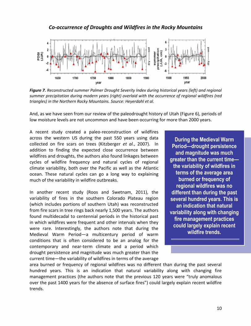
WILDFIRES There is a clear link between dry conditions and the outbreak of wildfires across the western United States, including the state of Utah. Figure 7 shows the co-occurrence of regional wildfire and dry conditions in the US Northern Rockies for the past several hundred years. Notice that most regional wildfire (red triangles) occur when conditions are dry (PDSI is below zero, or summer precipitation is less than normal). Most widespread wildfire outbreaks occur during times of low moisture levels.

10

Co-occurrence of Droughts and Wildfires in the Rocky Mountains

Figure 7. Reconstructed summer Palmer Drought Severity Index during historical years (left) and regional summer precipitation during modern years (right) overlaid with the occurrence of regional wildfires (red triangles) in the Northern Rocky Mountains. Source: Heyerdahl et al.

And, as we have seen from our review of the paleodrought history of Utah (Figure 6), periods of low moisture levels are not uncommon and have been occurring for more than 2000 years. A recent study created a paleo-reconstruction of wildfires across the western US during the past 550 years using data collected on fire scars on trees (Kitzberger et al., 2007). In addition to finding the expected close occurrence between wildfires and droughts, the authors also found linkages between cycles of wildfire frequency and natural cycles of regional climate variability, both over the Pacific as well as the Atlantic ocean. These natural cycles can go a long way to explaining much of the variability in wildfire outbreaks. In another recent study (Roos and Swetnam, 2011), the variability of fires in the southern Colorado Plateau region (which includes portions of southern Utah) was reconstructed from fire scars in tree rings back nearly 1,500 years. The authors found multidecadal to centennial periods in the historical past in which wildfires were frequent and other intervals when they were rare. Interestingly, the authors note that during the Medieval Warm Period—a multicentury period of warm conditions that is often considered to be an analog for the contemporary and near-term climate and a period which drought persistence and magnitude was much greater than the current time—the variability of wildfires in terms of the average area burned or frequency of regional wildfires was no different than during the past several hundred years. This is an indication that natural variability along with changing fire management practices (the authors note that the previous 120 years were “truly anomalous over the past 1400 years for the absence of surface fires”) could largely explain recent wildfire trends.

During the Medieval Warm Period—drought persistence

and magnitude was much greater than the current time—

the variability of wildfires in terms of the average area

burned or frequency of regional wildfires was no

different than during the past several hundred years. This is

an indication that natural variability along with changing

fire management practices could largely explain recent

wildfire trends.

11

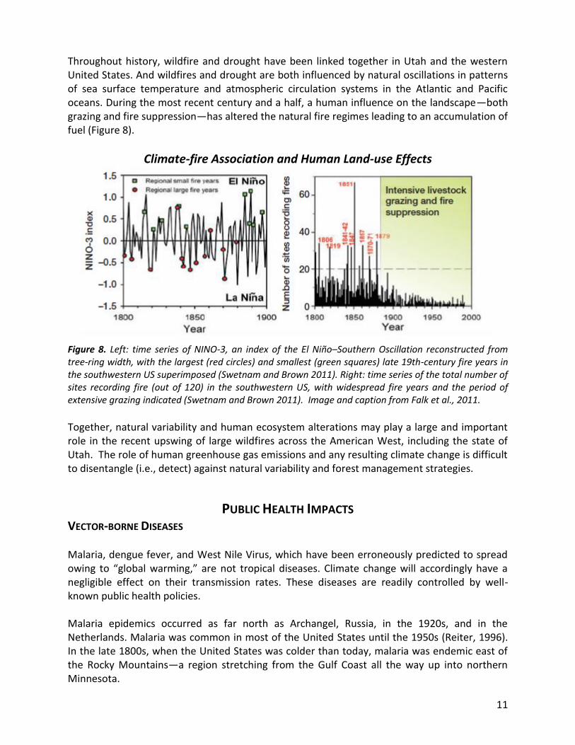
Throughout history, wildfire and drought have been linked together in Utah and the western United States. And wildfires and drought are both influenced by natural oscillations in patterns of sea surface temperature and atmospheric circulation systems in the Atlantic and Pacific oceans. During the most recent century and a half, a human influence on the landscape—both grazing and fire suppression—has altered the natural fire regimes leading to an accumulation of fuel (Figure 8).

Climate-fire Association and Human Land-use Effects

Figure 8. Left: time series of NINO-3, an index of the El Niño–Southern Oscillation reconstructed from tree-ring width, with the largest (red circles) and smallest (green squares) late 19th-century fire years in the southwestern US superimposed (Swetnam and Brown 2011). Right: time series of the total number of sites recording fire (out of 120) in the southwestern US, with widespread fire years and the period of extensive grazing indicated (Swetnam and Brown 2011). Image and caption from Falk et al., 2011.

Together, natural variability and human ecosystem alterations may play a large and important role in the recent upswing of large wildfires across the American West, including the state of Utah. The role of human greenhouse gas emissions and any resulting climate change is difficult to disentangle (i.e., detect) against natural variability and forest management strategies.

PUBLIC HEALTH IMPACTS VECTOR-BORNE DISEASES Malaria, dengue fever, and West Nile Virus, which have been erroneously predicted to spread owing to “global warming,” are not tropical diseases. Climate change will accordingly have a negligible effect on their transmission rates. These diseases are readily controlled by well-known public health policies. Malaria epidemics occurred as far north as Archangel, Russia, in the 1920s, and in the Netherlands. Malaria was common in most of the United States until the 1950s (Reiter, 1996). In the late 1800s, when the United States was colder than today, malaria was endemic east of the Rocky Mountains—a region stretching from the Gulf Coast all the way up into northern Minnesota.

12

In 1878, 100,000 Americans were infected with malaria, and some 25,000 died. Malaria was eradicated from the United States in the 1950s not because of climate change (it was warmer in the 1950s than in the 1880s), but because of technological advances. Air-conditioning, the use of screen doors and windows, and the elimination of urban overpopulation brought about by the development of suburbs and automobile commuting were largely responsible for the decline in malaria (Reiter, 1996).

Malaria Occurrence in the United States, 1880s

Figure 9. In the late 19th century malaria was endemic in shaded regions. Source: Reiter, 2001.

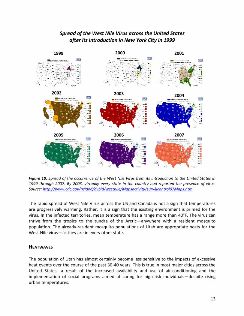
The effect of technology is also clear from statistics on dengue fever outbreaks, another mosquito-borne disease. In 1995, a dengue pandemic hit the Caribbean and Mexico. More than 2,000 cases were reported in the Mexican border town of Reynosa. But in the town of Hidalgo, Texas, located just across the river, there were only seven reported cases (Reiter, 1996). This is just not an isolated example. Data collected over the past decade have shown a similarly large disparity between incidence of disease in northern Mexico and in the southwestern United States, though there is very little climate difference. Another “tropical” disease that is often wrongly linked to climate change is the West Nile Virus. The claim is often made that a warming climate is allowing the mosquitoes that carry West Nile Virus to spread into Utah. This reasoning is incorrect. West Nile Virus, a mosquito-borne infection, was introduced to the United States through the port of New York in summer 1999. Since its introduction, it has spread rapidly, reaching the West Coast by 2002. Incidence has now been documented in every state as well as most provinces of Canada.

13

Spread of the West Nile Virus across the United States

after its Introduction in New York City in 1999

Figure 10. Spread of the occurrence of the West Nile Virus from its introduction to the United States in 1999 through 2007. By 2003, virtually every state in the country had reported the presence of virus. Source: http://www.cdc.gov/ncidod/dvbid/westnile/Mapsactivity/surv&control07Maps.htm.

The rapid spread of West Nile Virus across the US and Canada is not a sign that temperatures are progressively warming. Rather, it is a sign that the existing environment is primed for the virus. In the infected territories, mean temperature has a range more than 40°F. The virus can thrive from the tropics to the tundra of the Arctic—anywhere with a resident mosquito population. The already-resident mosquito populations of Utah are appropriate hosts for the West Nile virus—as they are in every other state.

HEATWAVES The population of Utah has almost certainly become less sensitive to the impacts of excessive heat events over the course of the past 30-40 years. This is true in most major cities across the United States—a result of the increased availability and use of air-conditioning and the implementation of social programs aimed at caring for high-risk individuals—despite rising urban temperatures.

2000 2001 1999

2002 2003 2004

2005 2006 2007

14

Heat-related Mortality Trends Across the US

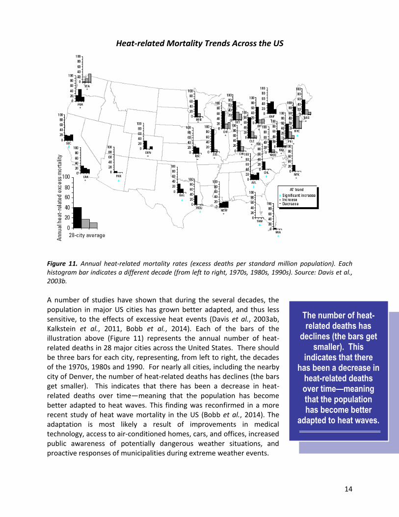
Figure 11. Annual heat-related mortality rates (excess deaths per standard million population). Each histogram bar indicates a different decade (from left to right, 1970s, 1980s, 1990s). Source: Davis et al., 2003b. A number of studies have shown that during the several decades, the population in major US cities has grown better adapted, and thus less sensitive, to the effects of excessive heat events (Davis et al., 2003ab, Kalkstein et al., 2011, Bobb et al., 2014). Each of the bars of the illustration above (Figure 11) represents the annual number of heat-related deaths in 28 major cities across the United States. There should be three bars for each city, representing, from left to right, the decades of the 1970s, 1980s and 1990. For nearly all cities, including the nearby city of Denver, the number of heat-related deaths has declines (the bars get smaller). This indicates that there has been a decrease in heat-related deaths over time—meaning that the population has become better adapted to heat waves. This finding was reconfirmed in a more recent study of heat wave mortality in the US (Bobb et al., 2014). The adaptation is most likely a result of improvements in medical technology, access to air-conditioned homes, cars, and offices, increased public awareness of potentially dangerous weather situations, and proactive responses of municipalities during extreme weather events.

The number of heat-related deaths has

declines (the bars get smaller). This

indicates that there has been a decrease in

heat-related deaths over time—meaning that the population has become better

adapted to heat waves.

15

The pattern of the distribution of heat-related mortality shows that in locations where extremely high temperatures are more commonplace, such as along the southern tier states, the prevalence of heat-related mortality is much lower than in the regions of the country where extremely high temperatures are somewhat rarer (e.g. the northeastern US). This provides another demonstration that populations adapt to their prevailing climate conditions. If temperatures warm in the future and excessive heat events become more common, there is every reason to expect that adaptations will take place to lessen their impact on the general population.

AIR POLLUTION Despite claims that “global warming” will increase the concentrations of air pollution across Utah and negatively impact human health, observations show the exact opposite has been going on during the past decade. The number of days in Salt Lake City, Utah with an “unhealthy” rating of the US Environmental Protection Agency’s Air Quality Index declined from 2002-2010 (EPA, 2011).

Air Quality Index Changes

Figure 12. Number of days with an Air Quality Index greater than 100 (a value above which is considered “unhealthy”) during 2002-2010. Source: Environmental Protection Agency, http://www.epa.gov/air/air trends/2011/index.html.

Despite claims that

“global warming” will

increase the

concentrations of air

pollution across Utah

and negatively impact

human health,

observations show the

exact opposite has

been going on during

the past decade.

16

The EPA reports more of the same, not just across Utah, but across much of the United States. Figure 12 shows the number of days with an Air Quality Index greater than 100 (a value considered “unhealthy”) during the period 2002-2010 for cities across the country. For the vast majority of these cities, the air quality has been improving—all during a period of increasing atmospheric greenhouse gas levels and “global warming.” According to the EPA “[g]iven the general improvement in air quality over the past decade, it appears that emissions reductions from air quality regulations are outpacing any climate-driven impacts” (EPA, 2011). This fact is driven home by another EPA analysis (Figure 13) which shows that, nationwide, the aggregate emissions of six common air pollutants declined by 62% since 1980, while the US gross domestic product rose by 145%, vehicle miles travelled increased by 95%, population grew by 39%, energy consumption expanded by 25% and carbon dioxide emissions increased by 14%. Clearly, factors other than human-caused climate change dominate the long-term and ongoing trends towards cleaner air.

Figure 13. Comparison of growth areas and emissions, 1980-2013. Source: EPA, http://www.epa.gov/air trends/aqtrends.html#comparison.

IMPACTS OF CLIMATE-MITIGATION MEASURES IN THE STATE OF UTAH

CLIMATE IMPACTS

Globally, in 2011, humankind emitted 32,154 million metric tons of carbon dioxide from the production of energy (mmtCO2: EIA, International Energy Statistics), of which emissions from Utah accounted for 63.9 mmtCO2, or just 0.20% (EIA, State CO2 Emissions). The global

17

proportion of manmade CO2 emissions from Utah will decrease over the 21st century as the rapid demand for power in developing countries such as China and India outpaces the growth of Utah’s CO2 emissions (EIA, International Energy Outlook). During the past 10 years, global emissions of CO2 from human activity have increased at an average rate of 3.1%/year (EIA, International Energy Statistics), meaning that the annual increase of anthropogenic global CO2 emissions is more than 15 times greater than Utah’s total emissions. This means that even a complete cessation of all CO2 emissions in Utah will be completely subsumed by global emissions growth in about one month’s time! In fact, China alone adds about 8 Utahs-worth of new emissions to its emissions total each and every year. Clearly, given the magnitude of the global emissions and global emission growth, regulations prescribing a reduction, or even a complete cessation, of Utah’s CO2 emissions will have absolutely no effect on global climate. Wigley (1998) examined the climate impact of adherence to the emissions controls agreed under the Kyoto Protocol by participating nations, and found that, if all developed countries meet their commitments in 2010 and maintain them through 2100, with a mid-range sensitivity of surface temperature to changes in CO2, the amount of warming “saved” by the Kyoto Protocol would be 0.07°C by 2050 and 0.15°C by 2100. The global sea level rise “saved” would be 2.6 cm, or one inch. A complete cessation of CO2 emissions in Utah is only a tiny fraction of the worldwide reductions assumed in Dr. Wigley’s global analysis, so its impact on future trends in global temperature and sea level will be only a minuscule fraction of the negligible effects calculated by Dr. Wigley. We now apply Dr. Wigley’s results to CO2 emissions in Utah, assuming that the ratio of US CO2 emissions to those of the developed countries which have agreed to limits under the Kyoto Protocol remains constant at 39% (25% of global emissions) throughout the 21st century. We also assume that developing countries such as China and India continue to emit at an increasing rate. Consequently, the annual proportion of global CO2 emissions from human activity that is contributed by human activity in the United States will decline. Finally, we assume that the proportion of total US CO2 emissions in Utah – now 1.2% – remains constant throughout the 21st century. With these assumptions, we generate the following table derived from Wigley’s (1998) mid-range emissions scenario (which itself is based upon the IPCC’s scenario “IS92a”):

The annual increase of

anthropogenic global CO2

emissions is more than

15 times greater than

Utah’s total emissions.

This means that even a

complete cessation of all

CO2 emissions in Utah

will be completely

subsumed by global

emissions growth in

about one month’s time!

Given the magnitude of

the global emissions and

global emission growth,

regulations prescribing a

reduction, or even a

complete cessation, of

Utah’s CO2 emissions will

have absolutely no effect

on global climate.

18

Table 1

Projected Annual CO2 Emissions (mmtCO2)

Year Global Emissions

(Wigley, 1998) Developed Countries

(Wigley, 1998) United States

(39% of developed countries)

Utah (1.2% of US)

2011 26,609 14,934 5,795 69

2025 41,276 18,308 7,103 85

2050 50,809 18,308 7,103 85

2100 75,376 21,534 8,355 100

Note: Developed countries’ emissions, according to Wigley’s assumptions, do not change between 2025 and 2050: neither does total US or Utah emissions.

In Table 2, we compare the total CO2 emissions saving that would result if Utah’s CO2 emissions were completely halted by 2025 with the emissions savings assumed by Wigley (1998) if all nations met their Kyoto commitments by 2010, and then held their emissions constant throughout the rest of the century. This scenario is “Kyoto Const.”

Table 2

Projected Annual CO2 Emissions Savings (mmtCO2)

Year Utah Kyoto Const.

2010 0 0

2025 85 4,697

2050 85 4,697

2100 100 7,924

Table 3 shows the proportion of the total emissions reductions in Wigley’s (1998) case that would be contributed by a complete halt of all Utah’s CO2 emissions (calculated as column 2 in Table 2 divided by column 3 in Table 2).

Table 3

Utah’s Percentage of Emissions Savings

Year Utah

2010 0.0%

2025 1.8%

2050 1.8%

2100 1.3%

Using the percentages in Table 3, and assuming that temperature change scales in proportion to CO2 emissions, we calculate the global temperature savings that will result from the complete cessation of anthropogenic CO2 emissions in Utah:

19

Table 4

Projected Global Temperature Savings (°C)

Year Kyoto Const. Utah

20100 0 0

2025 0.03 0.0005

2050 0.07 0.001

2100 0.15 0.002

Accordingly, a cessation of all of Utah’s CO2 emissions would result in a climatically-irrelevant global temperature reduction by the year 2100 of about two thousandths of a degree Celsius. Results for sea-level rise are also negligible:

Table 5

Projected Global Sea-level Rise Savings (cm)

Year Kyoto Const. Utah

2010 0 0

2025 0.2 0.004

2050 0.9 0.02

2100 2.6 0.03

A complete cessation of all anthropogenic emissions from Utah will result in a global sea-level rise savings by the year 2100 of an estimated 0.03 cm, or about 1 hundredths of an inch. Again, this value is climatically irrelevant. In this context, any cuts in emissions from Utah would be extravagantly pointless. Utah’s carbon dioxide emissions, in their sum total, effectively do not impact world climate in any way whatsoever.

A cessation of all of Utah’s CO2 emissions would result in a climatically-irrelevant

global temperature reduction by the year 2100 of about two

thousandths of a degree Celsius.

A complete cessation of all anthropogenic emissions from Utah will result in a

global sea-level rise savings by the year 2100 of an

estimated 0.03 cm, or about 1 hundredths of an inch.

Utah’s carbon dioxide emissions, in their sum total,

effectively do not impact world climate in any way

whatsoever.

20

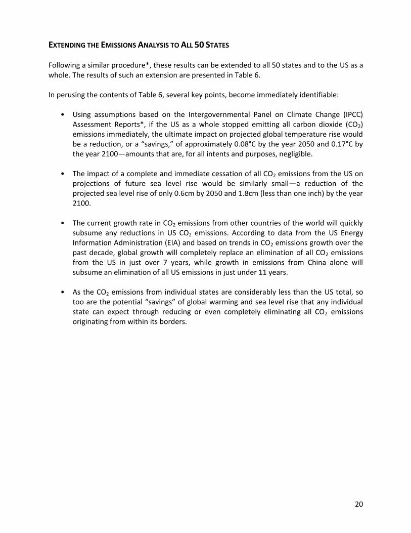
EXTENDING THE EMISSIONS ANALYSIS TO ALL 50 STATES Following a similar procedure*, these results can be extended to all 50 states and to the US as a whole. The results of such an extension are presented in Table 6. In perusing the contents of Table 6, several key points, become immediately identifiable:

• Using assumptions based on the Intergovernmental Panel on Climate Change (IPCC)

Assessment Reports*, if the US as a whole stopped emitting all carbon dioxide (CO2) emissions immediately, the ultimate impact on projected global temperature rise would be a reduction, or a “savings,” of approximately 0.08°C by the year 2050 and 0.17°C by the year 2100—amounts that are, for all intents and purposes, negligible.

• The impact of a complete and immediate cessation of all CO2 emissions from the US on

projections of future sea level rise would be similarly small—a reduction of the projected sea level rise of only 0.6cm by 2050 and 1.8cm (less than one inch) by the year 2100.

• The current growth rate in CO2 emissions from other countries of the world will quickly

subsume any reductions in US CO2 emissions. According to data from the US Energy Information Administration (EIA) and based on trends in CO2 emissions growth over the past decade, global growth will completely replace an elimination of all CO2 emissions from the US in just over 7 years, while growth in emissions from China alone will subsume an elimination of all US emissions in just under 11 years.

• As the CO2 emissions from individual states are considerably less than the US total, so

too are the potential “savings” of global warming and sea level rise that any individual state can expect through reducing or even completely eliminating all CO2 emissions originating from within its borders.

21

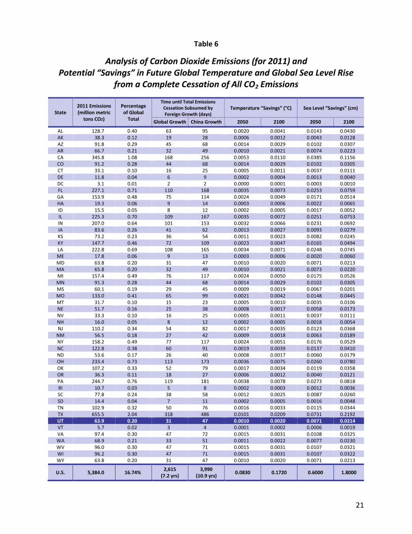
Table 6

Analysis of Carbon Dioxide Emissions (for 2011) and Potential “Savings” in Future Global Temperature and Global Sea Level Rise

from a Complete Cessation of All CO2 Emissions

State 2011 Emissions (million metric

tons CO2)

Percentage of Global

Total

Time until Total Emissions Cessation Subsumed by Foreign Growth (days)

Temperature “Savings” (°C) Sea Level “Savings” (cm)

Global Growth China Growth 2050 2100 2050 2100

AL 128.7 0.40 63 95 0.0020 0.0041 0.0143 0.0430 AK 38.3 0.12 19 28 0.0006 0.0012 0.0043 0.0128 AZ 91.8 0.29 45 68 0.0014 0.0029 0.0102 0.0307 AR 66.7 0.21 32 49 0.0010 0.0021 0.0074 0.0223 CA 345.8 1.08 168 256 0.0053 0.0110 0.0385 0.1156 CO 91.2 0.28 44 68 0.0014 0.0029 0.0102 0.0305 CT 33.1 0.10 16 25 0.0005 0.0011 0.0037 0.0111 DE 11.8 0.04 6 9 0.0002 0.0004 0.0013 0.0040 DC 3.1 0.01 2 2 0.0000 0.0001 0.0003 0.0010 FL 227.1 0.71 110 168 0.0035 0.0073 0.0253 0.0759 GA 153.9 0.48 75 114 0.0024 0.0049 0.0171 0.0514 HA 19.3 0.06 9 14 0.0003 0.0006 0.0022 0.0065 ID 15.5 0.05 8 12 0.0002 0.0005 0.0017 0.0052 IL 225.3 0.70 109 167 0.0035 0.0072 0.0251 0.0753 IN 207.0 0.64 101 153 0.0032 0.0066 0.0231 0.0692 IA 83.6 0.26 41 62 0.0013 0.0027 0.0093 0.0279 KS 73.2 0.23 36 54 0.0011 0.0023 0.0082 0.0245 KY 147.7 0.46 72 109 0.0023 0.0047 0.0165 0.0494 LA 222.8 0.69 108 165 0.0034 0.0071 0.0248 0.0745 ME 17.8 0.06 9 13 0.0003 0.0006 0.0020 0.0060 MD 63.8 0.20 31 47 0.0010 0.0020 0.0071 0.0213 MA 65.8 0.20 32 49 0.0010 0.0021 0.0073 0.0220 MI 157.4 0.49 76 117 0.0024 0.0050 0.0175 0.0526 MN 91.3 0.28 44 68 0.0014 0.0029 0.0102 0.0305 MS 60.1 0.19 29 45 0.0009 0.0019 0.0067 0.0201 MO 133.0 0.41 65 99 0.0021 0.0042 0.0148 0.0445 MT 31.7 0.10 15 23 0.0005 0.0010 0.0035 0.0106 NE 51.7 0.16 25 38 0.0008 0.0017 0.0058 0.0173 NV 33.3 0.10 16 25 0.0005 0.0011 0.0037 0.0111 NH 16.0 0.05 8 12 0.0002 0.0005 0.0018 0.0054 NJ 110.2 0.34 54 82 0.0017 0.0035 0.0123 0.0368

NM 56.5 0.18 27 42 0.0009 0.0018 0.0063 0.0189 NY 158.2 0.49 77 117 0.0024 0.0051 0.0176 0.0529 NC 122.8 0.38 60 91 0.0019 0.0039 0.0137 0.0410 ND 53.6 0.17 26 40 0.0008 0.0017 0.0060 0.0179 OH 233.4 0.73 113 173 0.0036 0.0075 0.0260 0.0780 OK 107.2 0.33 52 79 0.0017 0.0034 0.0119 0.0358 OR 36.3 0.11 18 27 0.0006 0.0012 0.0040 0.0121 PA 244.7 0.76 119 181 0.0038 0.0078 0.0273 0.0818 RI 10.7 0.03 5 8 0.0002 0.0003 0.0012 0.0036 SC 77.8 0.24 38 58 0.0012 0.0025 0.0087 0.0260 SD 14.4 0.04 7 11 0.0002 0.0005 0.0016 0.0048 TN 102.9 0.32 50 76 0.0016 0.0033 0.0115 0.0344 TX 655.5 2.04 318 486 0.0101 0.0209 0.0731 0.2192 UT 63.9 0.20 31 47 0.0010 0.0020 0.0071 0.0214 VT 5.7 0.02 3 4 0.0001 0.0002 0.0006 0.0019 VA 97.4 0.30 47 72 0.0015 0.0031 0.0108 0.0325 WA 68.9 0.21 33 51 0.0011 0.0022 0.0077 0.0230 WV 96.0 0.30 47 71 0.0015 0.0031 0.0107 0.0321 WI 96.2 0.30 47 71 0.0015 0.0031 0.0107 0.0322 WY 63.8 0.20 31 47 0.0010 0.0020 0.0071 0.0213

U.S. 5,384.0 16.74% 2,615

(7.2 yrs) 3,990

(10.9 yrs) 0.0830 0.1720 0.6000 1.8000

22

* The climate change calculations are performed using the MAGICC climate model simulator (MAGICC: Model for the Assessment of Greenhouse-gas Induced Climate Change; Wigley 2008). MAGICC was developed by scientists at the National Center for Atmospheric Research under funding by the US Environmental Protection Agency and other organizations. MAGICC is itself a collection of simple gas-cycle, climate, and ice-melt models that is designed to emulate the output of complex climate models. MAGICC produces projections of the global average temperature and sea level change under user configurable emissions scenarios and model parameters. There are many parameters that can be altered when running MAGICC, including the climate sensitivity (how much warming the model produces from a doubling of CO2 concentration) and the size of the effect produced by aerosols. In all cases, the MAGICC default settings were used (for example, a climate sensitivity of 3.0°C), which represent the middle-of-the-road estimates for these parameter values. Also, assumptions about the US emissions pathways were made as prescribed by the original IPCC scenarios in order to obtain the baseline US emissions to which the emissions reduction schedule could be applied—taking US emissions to zero (starting from 2010 levels) by the year 2020 and keeping them there to 2100 (the end of the simulation). The IPCC emissions scenarios describe the future emissions, not from individual countries, but from country groupings. Therefore, the US emissions were backed out from the country groupings. To do so, the country group which the US belonged to was identified (the OECD90 group) and then the current percentage of the total group emissions that are being contributed by the United States was determined—which turned out to be ~50%. The assumption was made that this percentage was constant over time. In other words, that the US contributed 50% of the OECD90 emissions in 2000 as well as in every year between 2000 and 2100. In this way, the future emissions pathway of the US was developed from the group pathway defined by the IPCC for each scenario (in this case, the A1B scenario). US carbon dioxide emissions were zeroed out by the year 2020 (but left all other emissions as defined by the A1B scenario) and then the new US emissions were recombined into the OECD90 pathway and into the global emissions total over time. It is the total global emissions that are entered into MAGICC in order to produce global temperature projections. The results using the zero-out US emissions pathway were then compared to the results using the original A1B pathways as prescribed by the IPCC. Once the projected climate (global average temperature and sea level) mitigation impacts of the zeroed out US emissions (compared with the original scenario) were calculated, the “savings” for each of the 50 United States was assigned in proportion to the percentage of total US carbon dioxide emitted within the borders of each state (based on 2010 emissions numbers published by the Energy Information Administration), with the assumption that these state-by-state proportions remained constant across the remainder of the 21st century.

ECONOMIC IMPACTS And what would be the potential costs to Utah of federal actions designed to reduce greenhouse gas emissions?

23

A comprehensive analysis was completed by the American Council for Capital Formation (ACCF) and the Small Business and Entrepreneurship Council (SBE) examining the economic impact of The American Power Act of 2010, also known as the Kerry-Lieberman bill. The Kerry-Lieberman bill is typical of federal proposal to reduce greenhouse gas emissions and so, even though this study is a few years old, it provides a good example of the economic impacts of stringent greenhouse gas restrictions. The ACCF/SBE commissioned the Science Applications International Corporation (SAIC) to assess the impact of the Kerry-Lieberman bill on industrial production, jobs, energy prices and the overall economy. The ACCF/SBE study accounts for all federal energy laws and regulations then in effect. It accounts for increased access to oil and natural gas supplies, new and extended tax credits for renewable generation technologies, as well as permit allocations for national and international offsets. Additionally, the provisions of the all federal government stimulus packages passed in 2008 and 2009 are included in the study. The 2010 American Power Act proposed targets that would reduce GHG emissions to 17% below 2005 levels by 2020; 42% below 2005 levels by 2030; and 83% below 2005 levels by 2050. For a complete description of these findings please visit: http://accf.org/accfsbe-council-study-on-kerry-lieberman-bill/. In general, for the US, the ACCF/SBE found:

Cumulative loss in Gross Domestic Product (GDP) ranging from $1.5 trillion to $2.1 trillion (2013-2030) depending on the cost assumption (low vs. high cost scenario)

Industrial production declines by between 4.9% and 5.8% by 2030 under the low and high cost scenarios

Employment losses up to 1.9 million jobs in 2030 even after additional “green” jobs are factored in

Residential electricity price increases by 29.3% to 42% percent by 2030

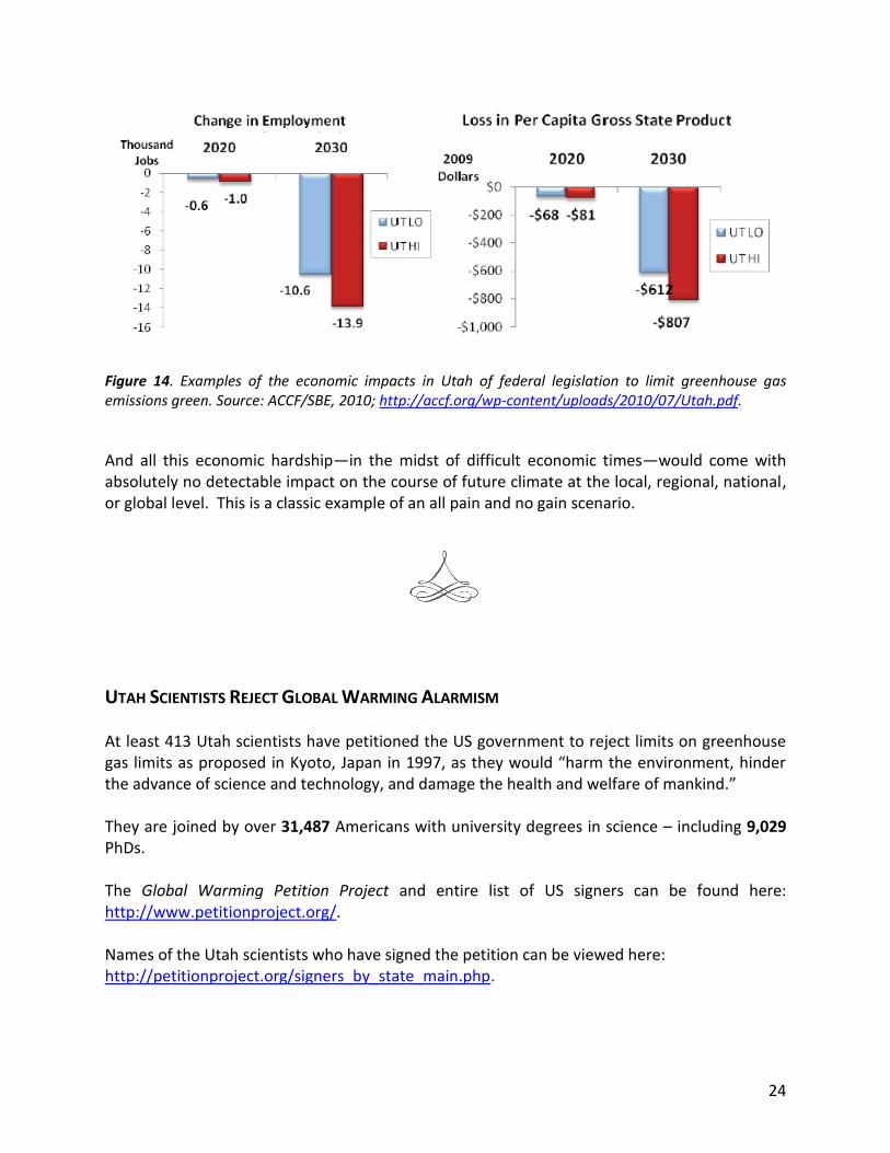
Gasoline price increases (per gallon) up to 18% percent by 2030. The ACCF/SBE also analyzed the economic costs on a state by state basis. For Utah, in particular, they found that by the year 2030, the state would stand to lose between 10,600 and 13,900 jobs. At the same time energy prices would rise substantially. Gasoline prices could increase by 18.5%, electricity prices by 47.2% and natural gas by up to 56.1%. Utah’s Gross State Product could decline by the year 2030 by between $5.4 and $7.2 billion/yr. with per capita Gross State Product falling during the same time by $612 to $807 per year.

By the year 2030, the state would stand to lose between

10,600 and 13,900 jobs.

This is a classic example of an all pain and no gain

scenario.

24

Figure 14. Examples of the economic impacts in Utah of federal legislation to limit greenhouse gas emissions green. Source: ACCF/SBE, 2010; http://accf.org/wp-content/uploads/2010/07/Utah.pdf.

And all this economic hardship—in the midst of difficult economic times—would come with absolutely no detectable impact on the course of future climate at the local, regional, national, or global level. This is a classic example of an all pain and no gain scenario.

UTAH SCIENTISTS REJECT GLOBAL WARMING ALARMISM At least 413 Utah scientists have petitioned the US government to reject limits on greenhouse gas limits as proposed in Kyoto, Japan in 1997, as they would “harm the environment, hinder the advance of science and technology, and damage the health and welfare of mankind.” They are joined by over 31,487 Americans with university degrees in science – including 9,029 PhDs. The Global Warming Petition Project and entire list of US signers can be found here: http://www.petitionproject.org/. Names of the Utah scientists who have signed the petition can be viewed here: http://petitionproject.org/signers_by_state_main.php.

25

REFERENCES Bobb, J.F., et al., 2014. Heat-related mortality and adaptation to heat in the United States. Environmental Health Perspectives, 122, 811-816, doi:10.1289/ehp.1307392. Cook, E.R., et al., 2008. North American Summer PDSI Reconstructions, Version 2a. IGBP PAGES/World Data Center for Paleoclimatology Data Contribution Series # 2008-046. NOAA/NGDC Paleoclimatology Program, Boulder CO, USA, ftp://ftp.ncdc.noaa.gov/pub/ data/paleo/drought/NAmericanDroughtAtlas.v2/readme-NADAv2-2008.txt. Energy Information Administration, International Energy Statistics, US Department of Energy, Washington, D.C., http://www.eia.gov/cfapps/ipdbproject/IEDIndex3.cfm?tid=90&pid=44 &aid=8, accessed February 19, 2015. Energy Information Administration, State CO2 Emissions, US Department of Energy, Washington, D.C., http://www.eia.gov/environment/emissions/state/state_emissions.cfm, accessed February 19, 2015, Energy Information Administration, 2014. International Energy Outlook 2014. US Department of Energy, Washington, D.C., http://www.eia.gov/forecasts/ieo/. Heyerdahl, E.K., et al., Multi-season climate synchronized widespread forest fires over four centuries (1630-2003), Northern Rocky Mountains USA. http://www.firescience.gov/ documents/Missoula_Posters/climate_syncronized_wildfire.pdf. Johnstone, J.A, and N. J. NMantua, 2014. Atmospheric controls on northeast Pacific temperature variability and change, 1900-2012. Proceedings of the National Academy of Sciences, 111, 14360-14365, doi:10.1073/pnas.1318371111. Kitzberger, T., et al., 2007. Contingent Pacific-Atlantic Ocean influence on multicentury wildfire synchrony over western North America. Proceedings of the National Academy of Sciences, 104, 543-548. Pielke Sr., R. A., et al., 2007. Documentation of uncertainties and biases associated with surface temperature measurement sites for climate change assessment. Bulletin of the American Meteorological Society, June 2007, 913-928. Reiter, P., 1996. Global warming and mosquito-borne disease in the USA. The Lancet, 348, 662. Reiter, P., 2001. Climate change and mosquito-borne disease. Environmental Health Perspectives, 109, 141-161. Roos, C.I., and T.W. Swetnam, 2011. A 1416-year reconstruction of annual, multidecadal, and centennial variability in area burned for ponderosa pine forests of the southern Colorado Plateau region, Southwest USA. The Holocene, 22, 281-290.

26

Swetnam T.W., and Brown, P.M., 2011. Climatic inferences from dendroecological reconstructions. In: Hughes MK, Swetnam TW, and Diaz HF (Eds). Dendroclimatology: progress and prospects. New York, NY: Springer Verlag. Watts, A., 2009. Is the US Surface Temperature Record Reliable? http://wattsupwiththat. files.wordpress.com/2009/05/surfacestationsreport_spring09.pdf. Wigley, T.M.L., 1998. The Kyoto Protocol: CO2, CH4 and climate implications. Geophysical Research Letters, 25, 2285-2288.