Ocean Surface Current Climatology in the Northern Gulf of Mexico by Donald R. Johnson Center for Fisheries Research and Development Gulf Coast Research Laboratory University of Southern Mississippi Project funded by the Marine Fisheries Initiative (MARFIN) program of NMFS/NOAA Published by Gulf Coast Research Laboratory Ocean Springs, Mississippi 39564 May 2008
Transcript
Ocean Surface Current Climatology in the Northern Gulf of Mexico
by
Donald R. Johnson
Center for Fisheries Research and Development Gulf Coast Research Laboratory
University of Southern Mississippi
Project funded by the
Marine Fisheries Initiative (MARFIN) program of NMFS/NOAA
Published by
Gulf Coast Research Laboratory Ocean Springs, Mississippi 39564
May 2008
ii
Table of Contents
List of Figures ………………………………………1
Abstract ………………………………………2
I. Introduction ………………………………………3
II. Data and Statistics ………………………………………4
A. Scalar ………………………………………6
B. Vector ……………………………………..10
III. Wind Stress Climatology ……………………………………14
IV. Surface Current Patterns ..….....……………………………20
A. Methodology ………...…………………………...20
B. Monthly Averaged Currents .......................................21
Acknowledgements ……………………………………..36
References ……………………………………..37
1
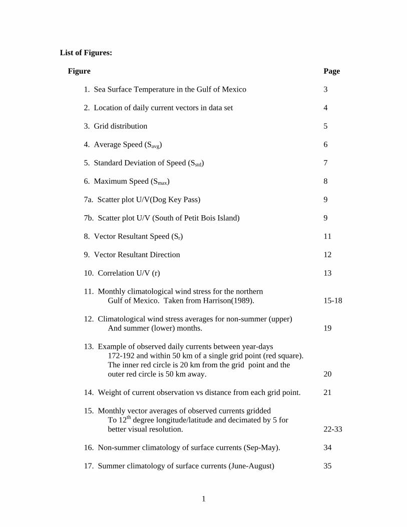
List of Figures:
Figure Page
1. Sea Surface Temperature in the Gulf of Mexico 3
2. Location of daily current vectors in data set 4
3. Grid distribution 5
4. Average Speed (Savg) 6
5. Standard Deviation of Speed (Sstd) 7
6. Maximum Speed (Smax) 8
7a. Scatter plot U/V(Dog Key Pass) 9
7b. Scatter plot U/V (South of Petit Bois Island) 9
8. Vector Resultant Speed (Sr) 11
9. Vector Resultant Direction 12
10. Correlation U/V (r) 13
11. Monthly climatological wind stress for the northern Gulf of Mexico. Taken from Harrison(1989). 15-18 12. Climatological wind stress averages for non-summer (upper) And summer (lower) months. 19 13. Example of observed daily currents between year-days 172-192 and within 50 km of a single grid point (red square). The inner red circle is 20 km from the grid point and the outer red circle is 50 km away. 20 14. Weight of current observation vs distance from each grid point. 21 15. Monthly vector averages of observed currents gridded To 12th degree longitude/latitude and decimated by 5 for better visual resolution. 22-33 16. Non-summer climatology of surface currents (Sep-May). 34 17. Summer climatology of surface currents (June-August) 35
2
Abstract
The goal of this technical report is to present a synthesis of 23 years of current observations on the continental shelves of the northern Gulf of Mexico (NGOM). As a result of several large Minerals Management Service programs, a rich set of satellite tracked drifter and moored current meter observations are available. These observations have been previously described in the literature (e.g., Ohlmann and Niiler, 2005 ). In this report, we add observations from other programs and synthesize the data set into statistical and circulation climatology for the continental shelves of the NGOM. This climatology is targeted especially for fishery researchers and managers who need to understand the effects of ocean currents on fishery problems. Both the scalar and vector (resultant) statistical synthesis of the entire set of near-surface currents are presented. Since wind stress plays a major role in establishing seasonal circulation patterns, monthly wind stress climatology has been taken from the literature (Harrison, 1989) and included here. The circulation climatology was formed from the observational data set by calculating daily current vectors and putting them into a year-day time frame (days 1-365) regardless of year. To elucidate patterns of currents, the data set was smoothed temporally (21-year-day moving window) and spatially (gridded by optimal interpolation). The result is a 365 day data set of surface current vectors, gridded at 1/12th degree longitude and latitude resolution. For presentation, this data set is averaged monthly and the results presented as monthly climatology. Since it has been noted that the circulation on the NGOM shelves can be separated into summer (June-August) and non-summer (rest of year) patterns, this climatology is included.
3
I. Introduction. The Northern Gulf of Mexico (NGOM) has been the site of several large observational programs involving measurements of ocean currents. A major goal for much of this work has been to develop a risk assessment for the NGOM involving oil spill spread by currents (Ohlmann and Niiler, 2005). As a result of these programs, a rich set of surface and near-surface current observations are available for other projects. Fishery programs involving larval transport, migratory patterns, aquaculture, marine protected areas, and the impact of climate change also need an understanding of fundamental circulation patterns and statistics of currents over broad regional areas. For example, the synthesized observational data described herein have previously been applied to the transport of red snapper (Lutjanus campechanus) larvae across the entire NGOM (Johnson et al., 2008). The goals of this technical report are to present the geographical distribution of observed current statistics and to describe and present the synthesis of observations into a current-climatology for the continental shelves of the NGOM. Over the continental shelf the principal driving forces are wind stress, buoyancy driven outflows, tides, and interactions with deep-basin events. Wind stress is important in driving the shallow waters over the shelf on both seasonal and storm scales (2-6 days in mid-latitudes). The Ekman Depth, or depth of wind stress momentum mixing, can represent a significant portion of the water column over the shelf. In addition, the near presence of the coastline and other boundaries contributes to rapid wind set-up and set-down. Buoyancy driven river and estuarine outflows also contain both seasonal and storm scales although storm scales are somewhat mitigated by interior drainage time. In the Gulf of Mexico, tidal currents are relatively small and require special handling for adequate resolution. They will not be further discussed in this report; however, they should be noted when assessing current forcing on structures and for short time scale (sub-diurnal) advection. Deep basin events and their effects on the continental shelf are difficult to predict, and can have substantial but transient impacts, particularly on the outer shelf and upper slope. Two major deep-basin circulation features created by basin geography and ocean dynamics are the Loop Current and spin-off rings (Figure 1). The Gulf of Mexico (GOM) is a semi-enclosed sea with inflow of North Atlantic/Caribbean Water through the Yucatan Channel. The Loop Current is formed when this inflow penetrates northward in the GOM before turning in an anti-cyclonic (clockwise) motion and exiting through the Straits of Florida. The loop at times turns back on itself and forms a ring, which eventually breaks off from the main flow. Under the influence of the earth’s rotation the separated ring migrates to the western basin. The rings are large and relatively deep; they spread warm, salty water through the central and western GOM, significantly affecting the oceanic and atmospheric climatology of the entire Gulf. Northward penetration of the loop and break-off of a ring, however, is a dynamically unstable process (Hurlbert and Thompson, 1980) with an unpredictable time scale of roughly 9-13 months (Vukovich, 1995). Since they do not contribute to seasonal patterns, these features affect current statistics but cannot be adequately captured in our
4
Spin-off ring
Loop Current
Figure 1: Sea surface temperature in Gulf of Mexico
climatology. Most of the action from the Loop Current and its rings are contained in the deep basin. However, it should be noted that they can interact with continental shelf waters, particularly over the outer shelf and upper slope region (Oey, 1995).
In this report, we 1.) Introduce the data set and derive current statistics. 2.) Present wind stress climatology. 3.) Present the methodology for determining circulation climatology. 4.) Present monthly and seasonal circulation climatology. II. Data and Statistics. The data set is derived from a variety of sources covering the period 1980-2002. Both satellite tracked drifters and moored current meters contributed to the set. Daily averaged current vectors were calculated from the drifters after interpolation along the drifter track to daily positions. Vector components (north and east positive) were formed from the daily positions and tagged with date and location. Moored current meters were both fixed level and Acoustic Doppler Current Profilers (ADCPs). Daily averages of near-surface currents were calculated for the moored instruments and each daily current vector component tagged with date and location. In the case of fixed level current meter
5
Figure 2
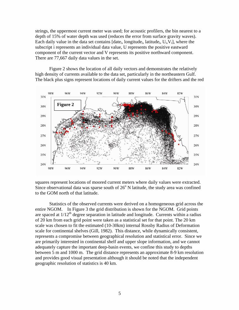
strings, the uppermost current meter was used; for acoustic profilers, the bin nearest to a depth of 15% of water depth was used (reduces the error from surface gravity waves). Each daily value in the data set contains [datei, longitudei, latitudei, Ui,Vi], where the subscript i represents an individual data value, U represents the positive eastward component of the current vector and V represents its positive northward component. There are 77,667 daily data values in the set. Figure 2 shows the location of all daily vectors and demonstrates the relatively high density of currents available to the data set, particularly in the northeastern Gulf. The black plus signs represent locations of daily current values for the drifters and the red
squares represent locations of moored current meters where daily values were extracted. Since observational data was sparse south of 26o N latitude, the study area was confined to the GOM north of that latitude. Statistics of the observed currents were derived on a homogeneous grid across the entire NGOM. In Figure 3 the grid distribution is shown for the NGOM. Grid points are spaced at 1/12th degree separation in latitude and longitude. Currents within a radius of 20 km from each grid point were taken as a statistical set for that point. The 20 km scale was chosen to fit the estimated (10-30km) internal Rossby Radius of Deformation scale for continental shelves (Gill, 1982). This distance, while dynamically consistent, represents a compromise between geographical resolution and statistical error. Since we are primarily interested in continental shelf and upper slope information, and we cannot adequately capture the important deep-basin events, we confine this study to depths between 5 m and 1000 m. The grid distance represents an approximate 8-9 km resolution and provides good visual presentation although it should be noted that the independent geographic resolution of statistics is 40 km.
6
Statistics of observed currents falls into two general categories: scalar and vector. Scalar values (regardless of direction) are more likely to be of importance where engineering parameters are needed for the effect of currents on structures. Vector (directional resultant) averages are more likely to be of importance where transport information is needed, e.g., larval advection or pollution dispersion. A. Scalar
Calculate speed, S, for all measured currents within 20 km of a grid point: Si = sqrt(Ui
2 + Vi2).
Where the indice, i, represents an individual current measurement within 20 km of the grid point, U is the positive eastward component of current speed and V is the positive northward component of current speed. Average speed: Savg = sum[Si]/N. Where N = number of current observations, i, within 20 k of the grid point. Standard deviation: Sstd = sqrt[sum(Si-Savg)2/(N-1)] Max Si: Smax = maximum(Si) Blank spaces in the following figures where Figure 3 shows a grid point indicate that there was and insufficient number of data points (N<4) to obtain a statistic at that grid point. Figure 4 shows the distribution of average speed, Savg, Figure 5 shows the distribution of standard deviation of the speed, Sstd, and Figure 6 shows the maximum speed, Smax, at each grid point.
Figure 3: Grid distribution
7
Figure 4: Average Speed (Savg)
8
Figure 5: Standard Deviation of Speed (Sstd)
9
Figure 6: Maximum Speed (Smax)
10
Figure 7a Figure 7b
B: Vector
Component speeds of each observed current value are found in the following manner. Ui = Si * sin(directioni) and Vi = Si * cos(directioni) Where directioni is the geographic direction of each current measurement within 20 km of grid point i. Calculate average U and average V: Uavg = sum(Ui)/N , Vavg = sum(Vi)/N. Calculate resultant current speed and direction: Sr = sqrt(Uavg
2 +Vavg2)
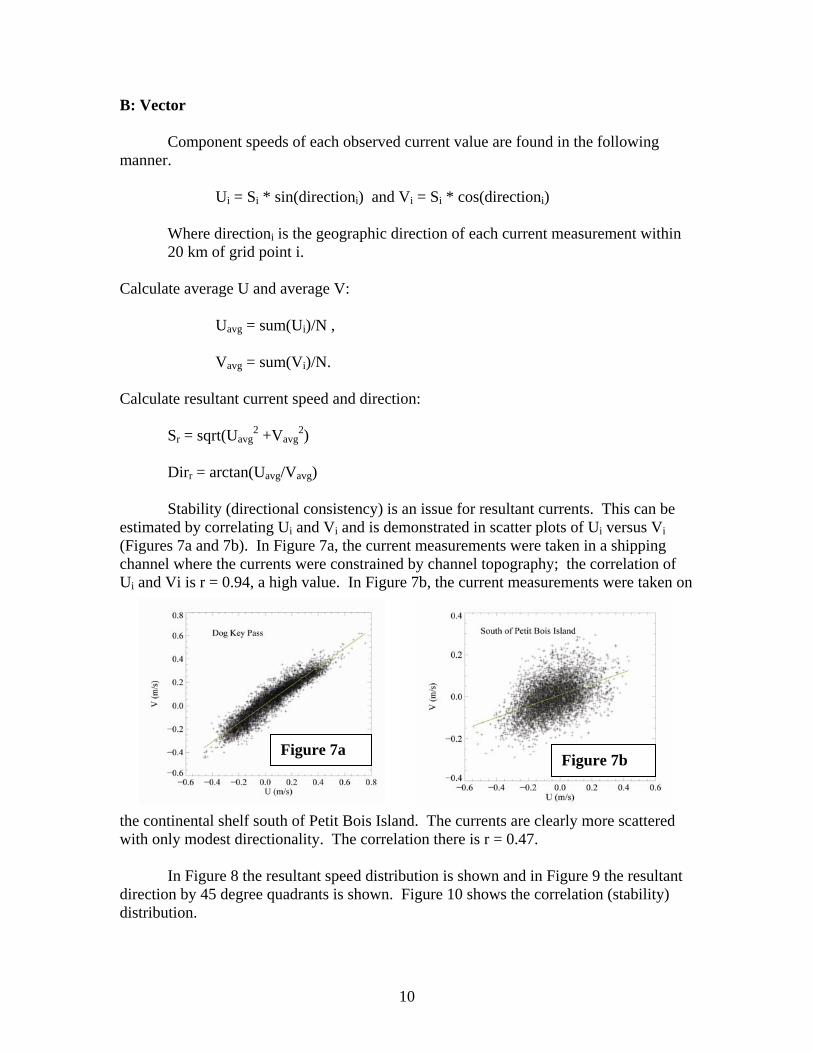
Dirr = arctan(Uavg/Vavg) Stability (directional consistency) is an issue for resultant currents. This can be estimated by correlating Ui and Vi and is demonstrated in scatter plots of Ui versus Vi (Figures 7a and 7b). In Figure 7a, the current measurements were taken in a shipping channel where the currents were constrained by channel topography; the correlation of Ui and Vi is r = 0.94, a high value. In Figure 7b, the current measurements were taken on
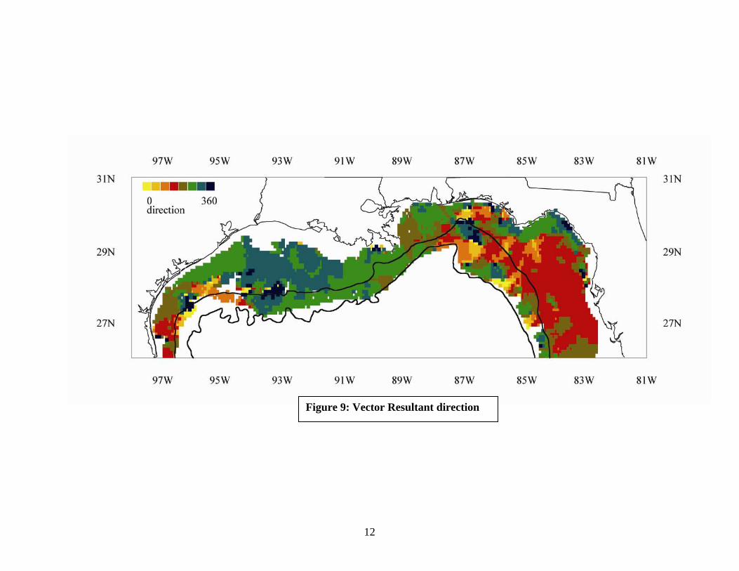
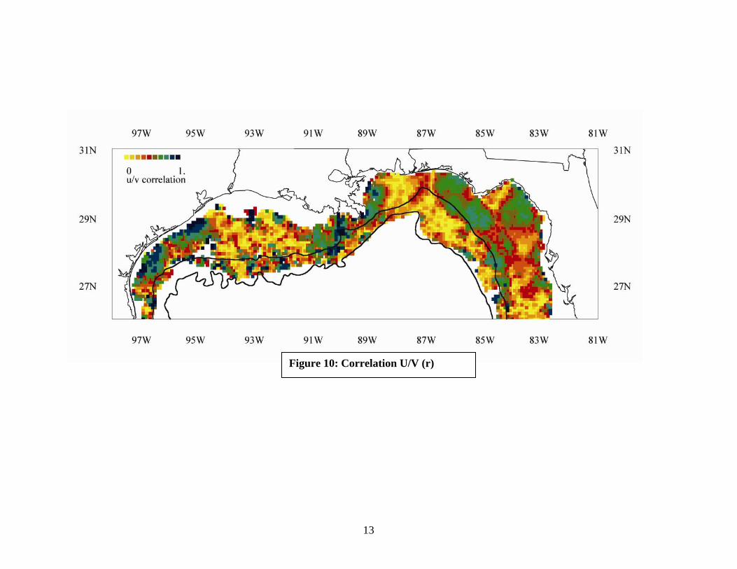
the continental shelf south of Petit Bois Island. The currents are clearly more scattered with only modest directionality. The correlation there is r = 0.47. In Figure 8 the resultant speed distribution is shown and in Figure 9 the resultant direction by 45 degree quadrants is shown. Figure 10 shows the correlation (stability) distribution.
11
Figure 8: Vector Resultant Speed (Sr)
12
Figure 9: Vector Resultant direction
13
Figure 10: Correlation U/V (r)
14
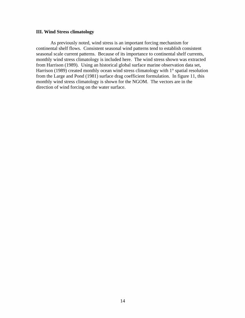
III. Wind Stress climatology
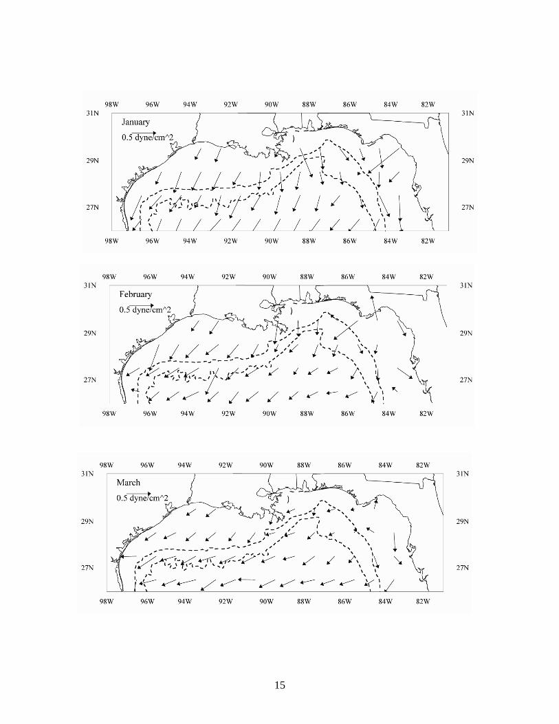
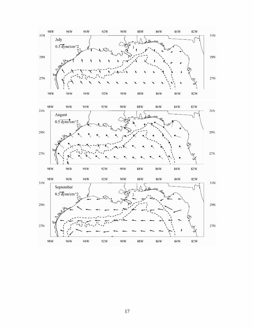
As previously noted, wind stress is an important forcing mechanism for continental shelf flows. Consistent seasonal wind patterns tend to establish consistent seasonal scale current patterns. Because of its importance to continental shelf currents, monthly wind stress climatology is included here. The wind stress shown was extracted from Harrison (1989). Using an historical global surface marine observation data set, Harrison (1989) created monthly ocean wind stress climatology with 1° spatial resolution from the Large and Pond (1981) surface drag coefficient formulation. In figure 11, this monthly wind stress climatology is shown for the NGOM. The vectors are in the direction of wind forcing on the water surface.
15
16
17
18
Figure 11: Monthly climatological wind stress for the northern Gulf of Mexico. Taken from Harrison (1989)
19
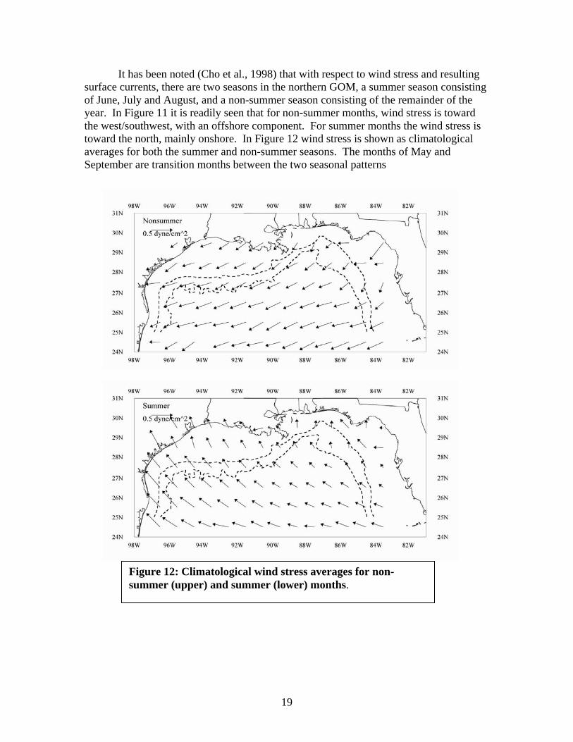
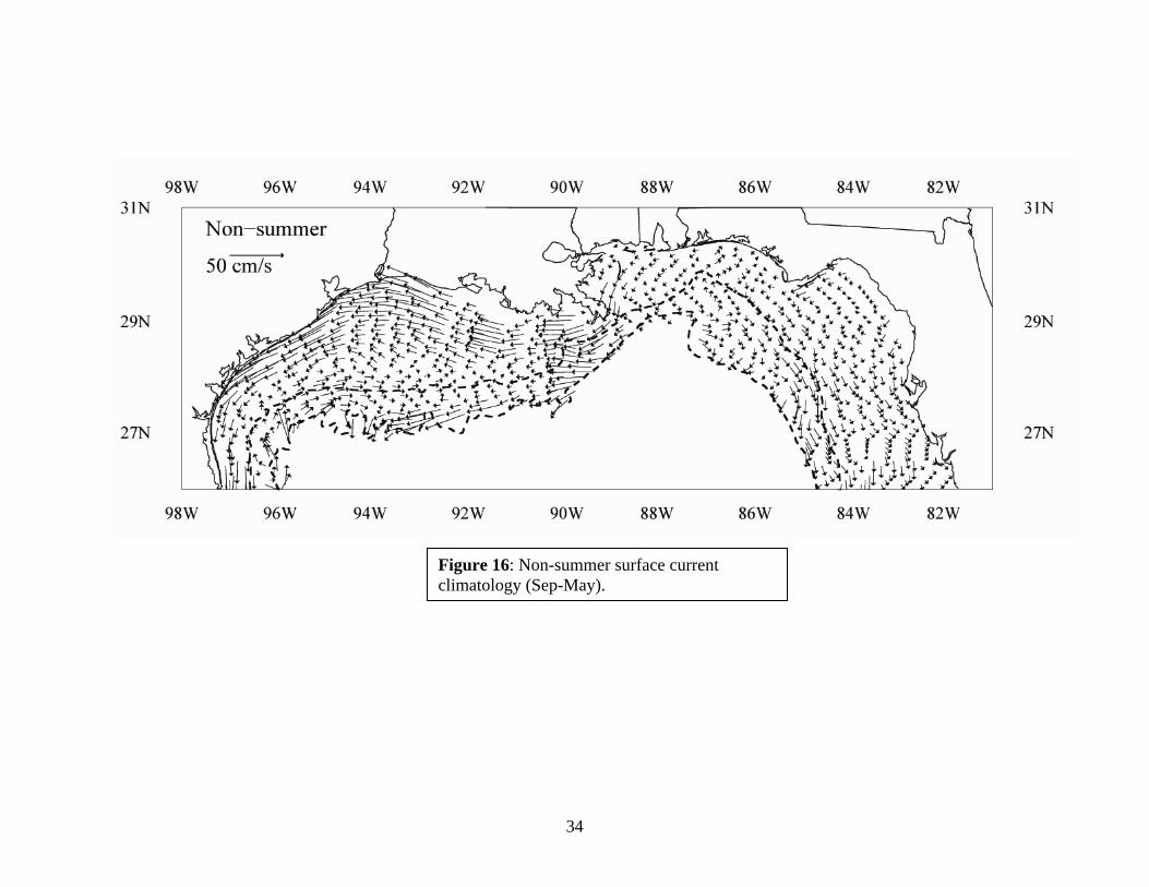
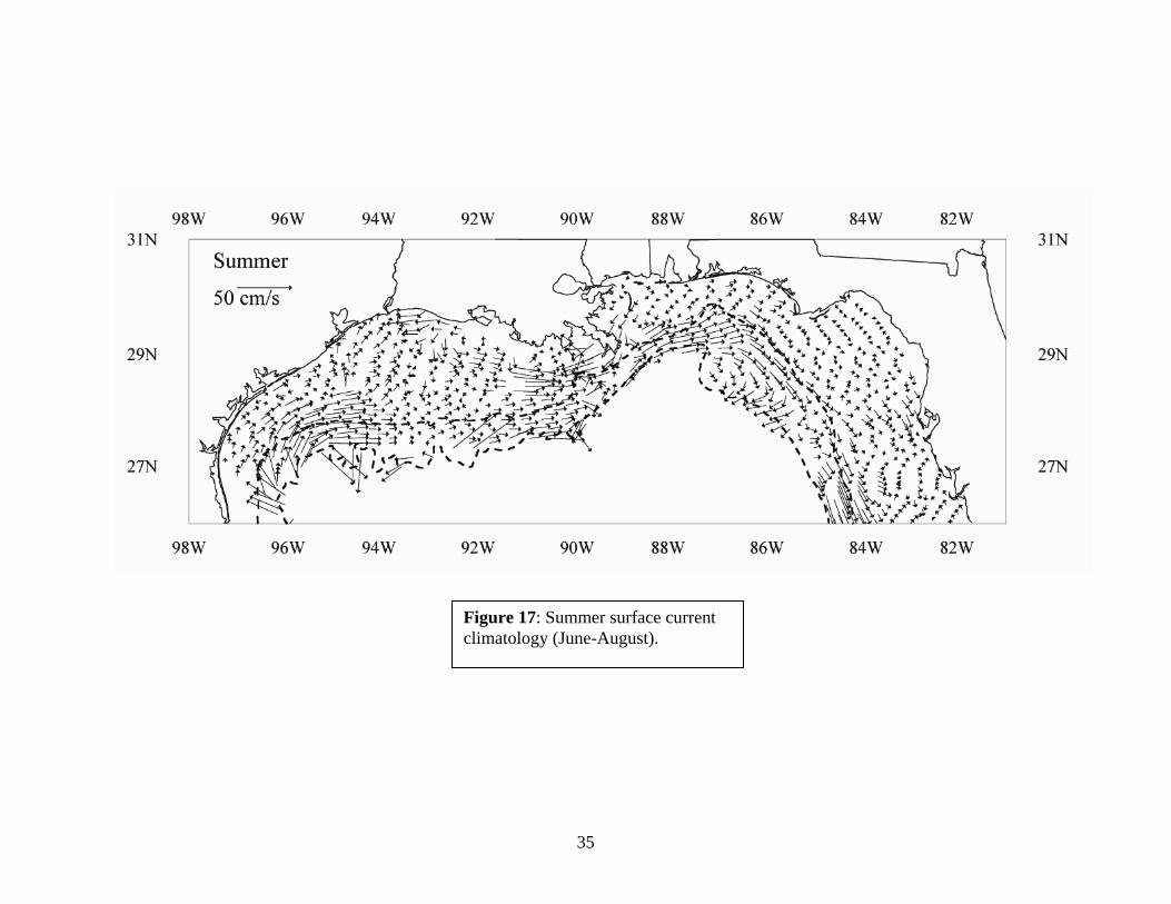
It has been noted (Cho et al., 1998) that with respect to wind stress and resulting surface currents, there are two seasons in the northern GOM, a summer season consisting of June, July and August, and a non-summer season consisting of the remainder of the year. In Figure 11 it is readily seen that for non-summer months, wind stress is toward the west/southwest, with an offshore component. For summer months the wind stress is toward the north, mainly onshore. In Figure 12 wind stress is shown as climatological averages for both the summer and non-summer seasons. The months of May and September are transition months between the two seasonal patterns
Figure 12: Climatological wind stress averages for non-summer (upper) and summer (lower) months.
20
Figure 13: Example of observed daily currents between year-days 172-192 and within 50 km of a single grid point (red square). The inner red circle is 20 km from the grid point and the outer red circle is 50 km away.
IV. Surface Current Patterns.
A. Methodology.
The surface current data set consists of observations made over a time span of 23 years with non-uniform horizontal spacing. In order to elucidate patterns of currents, the data set was smoothed in space and time. Each daily vector (n=77,667) was tagged with longitude, latitude and year-day (1-365) regardless of year, a moving window of 21-year-days was applied (temporal smoothing) and the current vectors in that 21-year-day window were interpolated to a uniform grid (spatial smoothing). Both temporal and spatial smoothing was accomplished as the data were gridded. Gridding was done at the same grid scale as in the statistical analysis (Figure 2). As an example of the gridding scheme, Figure 13 shows daily vector observations that fall within year-days 172 to 192, centered on year-day 182, and that are contained within 50 km of a single grid point at -88.5W and 29.5N. The vectors were interpolated to the grid point (red square in Figure 13) using an exponential weighting scheme (Bretherton et al., 1976): wi=exp(-di
2/rd2)
where di is the distance in km of vector i from the grid point and rd=20 km. The parameter rd, serves to establish how fast weighting diminishes with distance from the grid point. Statistically, the best choice of r would be from calculating the correlation length scale for currents at that point. However, with insufficient data to establish this length scale, it is estimated as the typical first mode baroclinic radius of deformation on continental shelves (10-30 km; Gill, 1982). A cut-off distance of 50 km applied before weighting prevents excessive, non-contributory calculations.
21
Figure 14: Weight of current observation vs distance from each grid point.
∑
∑ ×= n
ii
n
iii
j
w
Uwu
∑
∑ ×= n
ii
n
iii
j
w
Vwv
Figure 14 shows the value of weight, wi, applied to each observation versus distance from the grid point j. The individual weights are normalized by the sum of all weights applied at that grid point. The contribution of each observation to the calculated current value at the grid point is diminished rapidly with its distance away.
Current components uj and vj for grid point j, then, are formed in the following manner:
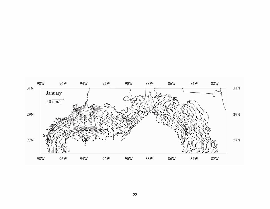
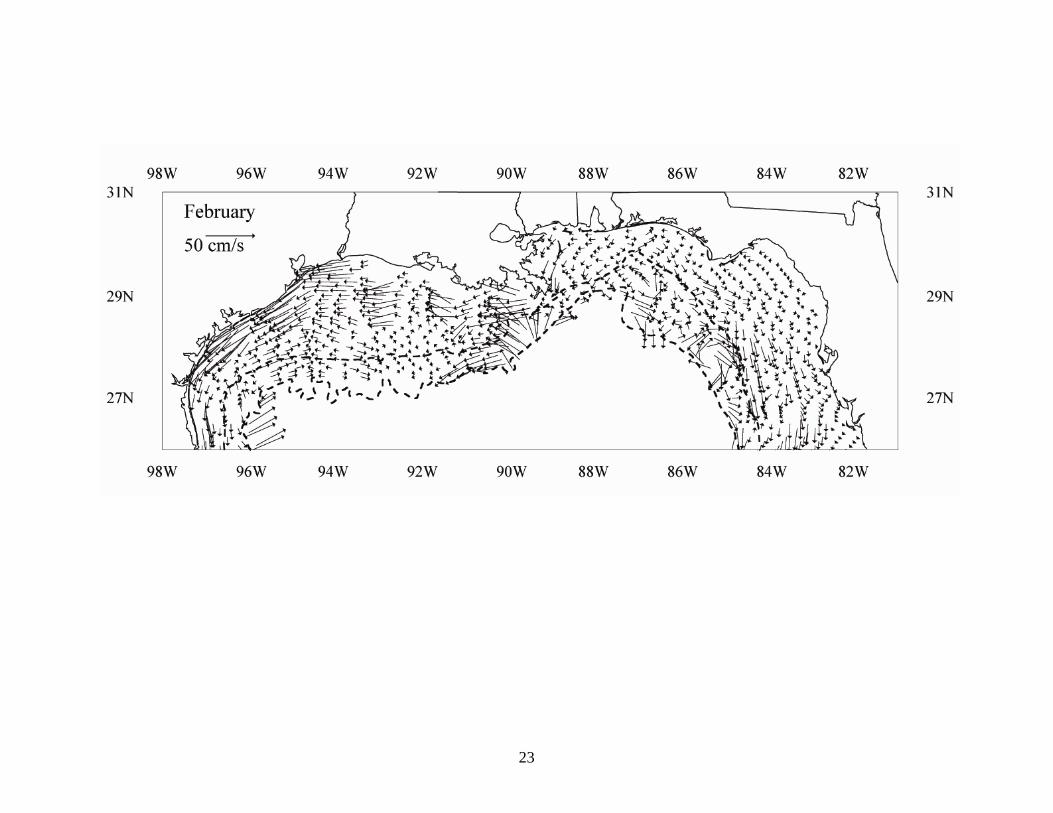
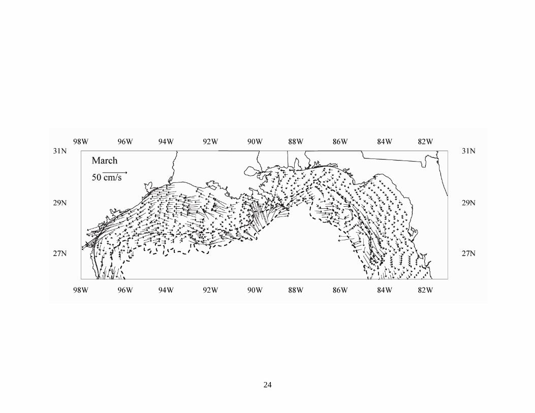
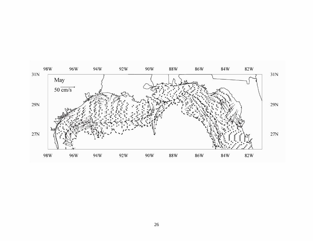
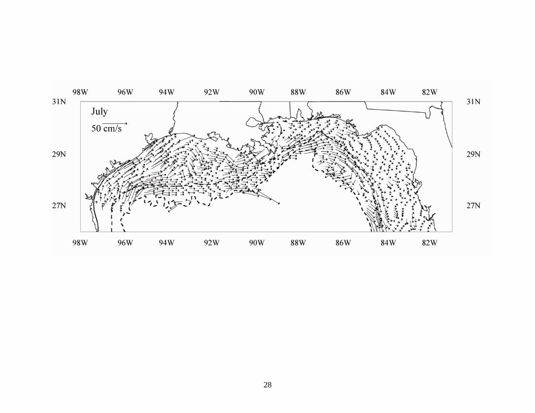
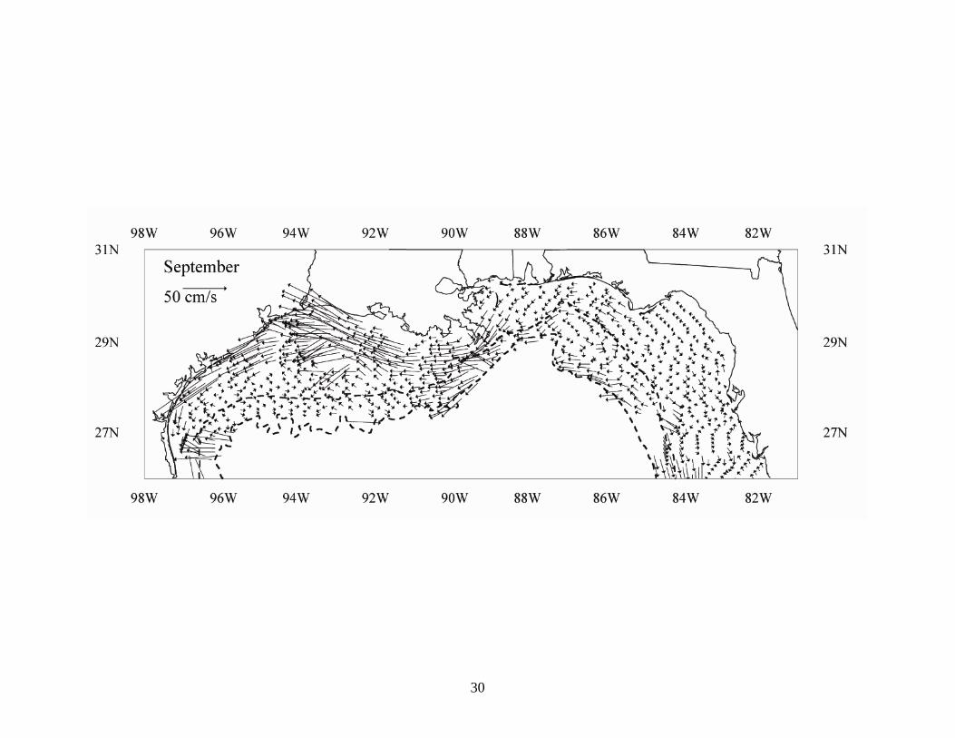
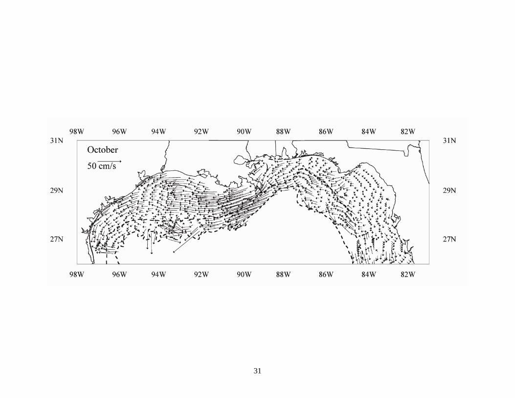
where j is the grid point indice and i is the indices of all observations within 50 km of grid point j. uj and vj are the resulting current components at grid point j. After currents have been computed at all grid points, the temporal 21-year-day window is moved over by one day, and currents are calculated for the new year-day. As the end of the year is reached in December, the 21-year-day window is wrapped around to January. B. Monthly Averaged Currents The calculated climatology then consists of 365 current values for each grid point. In order to display the results, monthly vector averages were made. Due to the density of grid points, the resulting vector averages were spatially decimated by a factor of 5 for display purposes. Figure 15 shows the vector monthly averages.
22
23
24
25
26
27
28
29
30
31
32
33
Figure 15: Monthly vector averages of observed currents gridded to 1/12th degree longitude/latitude and decimated by 5 for better visual resolution.
34
Figure 16: Non-summer surface current climatology (Sep-May).
35
Figure 17: Summer surface current climatology (June-August).
36
Acknowledgements
We gratefully acknowledge funding for this study from the Marine Fisheries Initiative (MARFIN) program of NMFS/NOAA, Southeastern Regional Office. The study would not have been possible without the generous contribution of data from a number of research scientists. Many of the current observations are from several large Minerals Management Service (MMS) projects in the northern GOM. We would especially like to acknowledge W. Johnson (MMS) and P. Niiler (Scripps Institution of Oceanography). Other programs involved W. Sturges (Florida State University) and R. Weisberg (University of South Florida). Drifter and moored current data were provided by J. Blaha, C. Szczechowski and S. Dinnel (Naval Oceanographic Office). A number of research scientists at Texas A&M and Louisiana State University contributed to a CD-ROM data set available through the National Oceanographic Data Center.
37
References
Bretherton F.P., R.E. Davis and C.B. Fandry (1976): A Technique for Objective Analysis and Design of Oceanic Experiments applied to MODE-73. Deep Sea Research, 23, p. 559-582.
Cho, K., R. O. Reid, W. D. Nowlin Jr. 1998. Objectively mapped stream function fields on the Texas-Louisana shelf based on 32 months of moored current meter data. J. Geophys. Res 103(C5): 10377-10390.
Gill, A. E. 1982. Atmosphere-Ocean Dynamics. Academic Press. New York. Harrison, D. E. 1989. On climatological monthly mean wind stress and wind stress curl
fields over the world ocean J. Climate 2(1): 57-70. Hurlbert, H. E. and J. D. Thompson. 1980. A numerical study of Loop Current
intrusions and eddy shedding. J. Phys. Oceanogr. 10: 1611-1651. Johnson, D. R., H. M. Perry, J. Lyczkowski-Shultz, D. Hanisko. 2008. Red snapper
(Lutjanus campechanus) larval transport in the northern Gulf of Mexico. Submitted Trans. Amer. Fish.
Large, W.G., and S. Pond, 1981: Open ocean momentum flux measurements in moderate to strong winds. J. Phys. Oceanogr., 11, 324-336. Oey, I. 1995. Eddy- and wind-forced shelf circulation. J. Geophys. Res. 100: 8621-8637. Ohlmann, J. C., P. P. Niiler. 2005. Circulation over the continental shelf in the northern
Gulf of Mexico. Prog. In Oceanogr., 64: 45-81 Vukovich, F. M. 1995. An updated evaluation of the Loop Current’s eddy-shedding