Accepted Manuscript

Observing the thermodynamic effects in cavitating flow by IR thermography

Martin Petkovšek, Matevž Dular

PII: S0894-1777(17)30197-8DOI: http://dx.doi.org/10.1016/j.expthermflusci.2017.07.001Reference: ETF 9143

To appear in: Experimental Thermal and Fluid Science

Received Date: 24 October 2016Revised Date: 1 June 2017Accepted Date: 2 July 2017

Please cite this article as: M. Petkovšek, M. Dular, Observing the thermodynamic effects in cavitating flow by IRthermography, Experimental Thermal and Fluid Science (2017), doi: http://dx.doi.org/10.1016/j.expthermflusci.2017.07.001

This is a PDF file of an unedited manuscript that has been accepted for publication. As a service to our customerswe are providing this early version of the manuscript. The manuscript will undergo copyediting, typesetting, andreview of the resulting proof before it is published in its final form. Please note that during the production processerrors may be discovered which could affect the content, and all legal disclaimers that apply to the journal pertain.

Observing the thermodynamic effects in cavitating flow by IR thermography

Martin Petkovšek* Laboratory for Water and Turbine Machines, University of Ljubljana, Aškerčeva 6, 1000 Ljubljana,

Slovenia

Matevž Dular Laboratory for Water and Turbine Machines, University of Ljubljana, Aškerčeva 6, 1000 Ljubljana,

Slovenia *Corresponding author Abstract When dealing with liquid flows, where operating temperature gets close to the liquid critical temperature, cavitation cannot be assumed as an isothermal phenomenon. Due to the relatively high density of vapor, the thermodynamic effect (decrease of temperature in the bulk liquid due to latent heat flow) becomes considerable and should not be neglected. For applications like pumping cryogenic fuel and oxidizer in liquid propulsion space launchers, consideration of the thermodynamic effect is essential - consequently the physical understanding of the phenomenon and its direct experimental observation has a great value. This study presents temperature measurements in a cavitating flow on a simple convergent-divergent constriction by infrared (IR) thermography. Developed cavitating flow of hot water (~100°C) was evaluated by high-speed IR thermography and compared with conventional high-speed visualization, at different operating conditions with the velocity range at the nozzle throat between 9.6 and 20.6 m/s and inlet pressure range between 143 and 263 kPa. Temperature depression near the nozzle throat - near the leading edge of cavitation was measured in a range up to ∆T=0.5 K. This confirms the presence of the thermodynamic effects by cavitation phenomenon and it is in agreement with its theory. In the study, average temperature fields, fields of temperature standard deviation and time-resolved temperatures, are presented and discussed. In addition, statistical analysis between temperature drop and cavitation flow characteristics is shown. Key words: thermodynamic effect, cavitation, temperature measurements, thermography, convergent-divergent nozzle 1 Introduction Cavitation, a physical phenomenon driven by local pressure drop in a liquid, is characterized by growth and collapse of small vapor-gas bubbles. In most cases, when for example we are dealing with cold water flow, one can assume the cavitation being an isothermal process. But it is known, that the cavity growth is driven mainly by the evaporation process, where the supplied latent heat from cavity surrounding causes a small temperature drop of the liquid, which results in a local drop of a vapor pressure. Further development of the bubble is now weakened or delayed, thus greater pressure drop is needed to maintain the cavity growth. This is known as the thermodynamic effect or thermal delay phenomenon and has a direct influence on the bubble dynamics. The effect becomes important when the operating temperature is close to the end point of a phase equilibrium curve (critical point) of the liquid – for example in cryogenic liquid flow. The latter is of an extreme interest to the scientists and engineers due to its usage in liquid propulsion space launch vehicles – there is a well-known example of space launch failure of Japanese H-II rocket due to the cavitation instability in the liquid hydrogen

pump [1]. The first experimental study, where the aspect of the thermodynamic effect was considered, was conducted by Stahl and Stepanoff [2]. Sarosdy and Acosta [3] noticed the difference in the appearance between the cavitation in water and cooling liquid Freon, but they were unable to physically explain it. Stepanoff [4] and Ruggeri and Moore [5] were the first, who experimentally quantified the phenomena and derived the correlations based on the so-called B-factor. Hord el al. [6] and Hord [7,8] conducted extensive experimental studies, where cavitation in liquid hydrogen, liquid nitrogen and refrigerant R114 was observed on Venturi profiles, hydrofoils and ogive models. Brennen [9] proposed the thermodynamic parameter Σ based only on fluid properties. Similar parameter α was proposed by Kato [10] and Σ* by Watanabe et al. [11]. Franc et al. [12–14] conducted several experiments on the inducer of the rocket motor turbopump with refrigerant R114 to forecast the characteristics of cavitation in the liquid hydrogen. Similarly, other researchers like Ito et al. [15], Cervone et al. [16], Yoshida et al. [17] and Kikuta et al. [18], all just observed cavitation with distinct presence of thermodynamic effect and its consequences, rather than investigating the mechanism itself. Rimbert et al. [19] conducted one of the first experimental measurements of the temperature in a cavitating flow within a microcavitation channel by two-color laser in several points. Ayela et al. [20] used thermosensitive fluorescent nanoparticles seeded in water to determine thermal gradients by cavitating flow in a microchannel. While Dular and Coutier-Delgosha [21] used high-speed IR thermography to measure the 2D temperature field on a large (several millimeters in diameter) single cavitation bubble, Petkovšek and Dular [22] conducted the first 2D temperature measurements on a cavitating flow in Venturi tube, also by IR thermography. Watanabe et al. [23] performed temperature measurements in liquid, hydrofluoro-ether, within Venturi tube, with six thermocouples. Despite significant progress in the recent years there is still a void in fundamental understanding of the thermodynamic effect in cavitating flow. The most challenging part by cavitation bubble is defining when and in what extent the expansion/evaporation part take place by bubble growth and condensation/compression by bubble collapse. Which mechanism prevails at certain stage of bubble lifetime is still not fully understood as well as in what ratio vapor and gas forms the bubble. Most attempts to numerically predict cavitating flow with consideration of thermodynamic effects base on comparison to the results from experimental studies performed in 1960’s and 70’s [24–28]. Since the temperature measurements in cavitating flows are rare and performed in one or at best in few measurement points, the numerical predictions of 2D temperature fields can be questionable. Thus new experimental studies with temperature measurements are vital for further development of new advanced numerical models. The present study deals with direct measurements of thermodynamic effects in cavitating flow (in hot water at approximately 100°C) within a simple convergent-divergent constriction. Since water at 20°C cannot be considered as a thermosensible liquid, heated up to 100°C can be used as a surrogate liquid for cryogenics to investigate thermodynamic effects (based on thermodynamic parameter Σ, Σ = 1 m/s3/2 (water at 20°C), Σ = 103 m/s3/2 (water at 100°C) [29]). In order to prevent water from boiling, all the measurements were performed at pressures above atmospheric pressure. For the first time the thermodynamic effects were observed by means of simultaneous high-speed visualization and high-speed IR thermography from both the side and bottom view. The results are valuable for deeper understanding of the phenomenon and very important for development and evaluation of advanced cavitation numerical models.

2 Theory Cavitation bubble evolution can be roughly divided into two regimes the inertial and thermal regime. While in case where heat transfer is negligible (e.g. in cold water), the phase change can be assumed driven mostly by inertial effects. However, when thermal effects are present (e.g. in cryogenics) the inertial part can become neglected [30,31]. The simple intuitive description of the spherical cavitation bubble behavior in an infinite liquid, from the initial nucleus till the bubble collapse into the bulk liquid, can be divided into six periods:

- Initial growth: Due to local pressure drop in the liquid near the nucleus, the gases inside the nucleus expand (inertial regime), what causes the bubble interior to cool. The temperature difference initiates the heat flow from the liquid to the bubble interface.

- Bubble growth: After the initial stage (gas expansion due to inertial forces), the process of vaporization prevails when the bubble growth rate decreases to allow the heat from the surrounding liquid to reach the bubble interface – the process can be considered close to isothermal. Bubble growth can be characterized as a thermal regime.

- Maximum bubble size: Bubble grows due to vaporization process until the maximum size is reached, at this point it is filled mostly by vapor.

- Collapsing: At the maximum size point, the heat flux stops and due to inertia moment, the bubble starts to collapse. The water vapor inside the bubble condensates, which causes a release of heat back to the surrounding liquid – thermal regime.

- Final collapsing stage: Bubble collapse accelerates and as it reaches the critical collapsing velocity (when the adiabatic process prevails over the isothermal), the temperature inside the bubble increases rapidly due to severe gas compression – inertial regime.

- Rebound: After the bubble collapse into the bulk liquid, the bubble can goes through several rebound stages, due to oscillating pressure field in the near surrounding liquid.

By assuming, that isothermal process (vaporization and condensation) prevails during bubble life time [32], the theory of Brennen [29] and Franc & Michel [33] gives us the following approximate relation between the liquid temperature on the bubble interface (Tb) and the ambient liquid temperature (T∞):

pll

v

l

bc

L

t

RTT

ρ

ρ

α ∆−=− ∞ , (1)

where ∆t is time in which bubble reaches its radius R, αl is thermal diffusivity, L presents latent heat, cpl presents the heat capacity at constant pressure in the liquid and ρl and ρv liquid and vapor density. In terms of vapor pressure difference the thermodynamic effect can be expressed as:

( )

∞∆=∆

Tc

L

t

Rp

pll

v

l

vρ

ρ

α

2

. (2)

Expression for the decrease of the vapor pressure ∆pv can be used in the Rayleigh-Plesset equation – including thermal effects [34]:

R

R

R

S

R

RppTpRRR gbvl

•

∞

•••

−−

+−=

+ µρ

γ

42

)(2

33

00

2

, (3)

Where the vapor pressure at bubble temperature can be defined by the vapor pressure at bulk liquid

temperature and vapor pressure difference due to the thermal delay:

vvbv pTpTp ∆−= ∞ )()( (4)

and with consideration of the Σ parameter [29]:

( )

lpll

v

Tc

L

αρ

ρ

∞

=Σ2

2

, (5)

it finally leads to:

R

R

R

S

R

RppTptRRRR gvll

•

∞∞

••••

−−

+−=Σ+

+ µρρ

γ

42

)(2

33

00

2

. (6)

The last equation gives us the bubble radius evolution in time, which can be used to calculate the time evolution of the temperature Tb from Eq. 1 (and measured during this study). Using Eq. 1 one can estimate the expected temperature depression for the present study. It was observed that the bubble reaches a maximum diameter of 50 µm, this occurs about 5 to 10 mm downstream of the throat of the Venturi. Considering the flow velocity in this region the time can be estimated to about 1 ms. Using the water parameters at 100°C one comes up to the expected temperature difference of CTTb °−=− ∞ 6.0 .

3 Experimental set-up Cavitation tests were conducted in a cavitation tunnel at the Laboratory for Water and Turbine machines, University of Ljubljana. 3.1 Cavitation tunnel The cavitation tunnel (Fig. 1) has a closed circuit which enables to vary the system pressure and the temperature of the liquid, tap water in our case. Circulation of the water is obtained by a 4.5 kW pump (1) with variable speed driver, which can deliver desired flow rate. At the pump delivery, a tank (2) partially filled with the circulation water is used for i) water heating (a 10 kW electric heater (3) is installed), and ii) attenuating the possible fluctuations in the flow rate and pressure due to the passage of the pump blades. Cavitation and thermodynamic effects are observed in a transparent polycarbonate test section (4). The tank downstream (5) of the test section is used for optional cooling of the circulation water - cooling water flows inside the tank in a secondary loop, which is connected to cold tap water. To provide high accuracy measurements, the temperature of the water is monitored by a Pt100 class A sensor (6), with 6 mm in diameter and stated accuracy of +/- 0.15 + 0.002 × T[°C], installed in the downstream tank and by a thermocouple J type, with 1.5 mm in diameter, installed directly into the test section, with stated accuracy of +/- 0.4%. The pressure inside the cavitation tunnel is monitored by two ABB 2600T pressure gauges (absolute and differential) and it can be varied by operating a vacuum pump and a compressor which were both connected to the downstream or upstream tank – such a set-up provides a wide range of hydrodynamic conditions. The uncertainty of the pressure measurements was +/- 800 Pa. Additionally, the flow rate can be controlled by two valves, installed

upstream and downstream of the test section. The volume flow rate is measured by electromagnetic flow meter ABB ProcessMaster 300 (7), which withstands the temperatures up to 180°C and provides an accuracy of 0.4%. The volume of the cavitation tunnel is approximately 100 liters and, in order to provide minimal temperature oscillations of the working fluid, the station is thermally insulated.

Figure 1: Cavitation tunnel

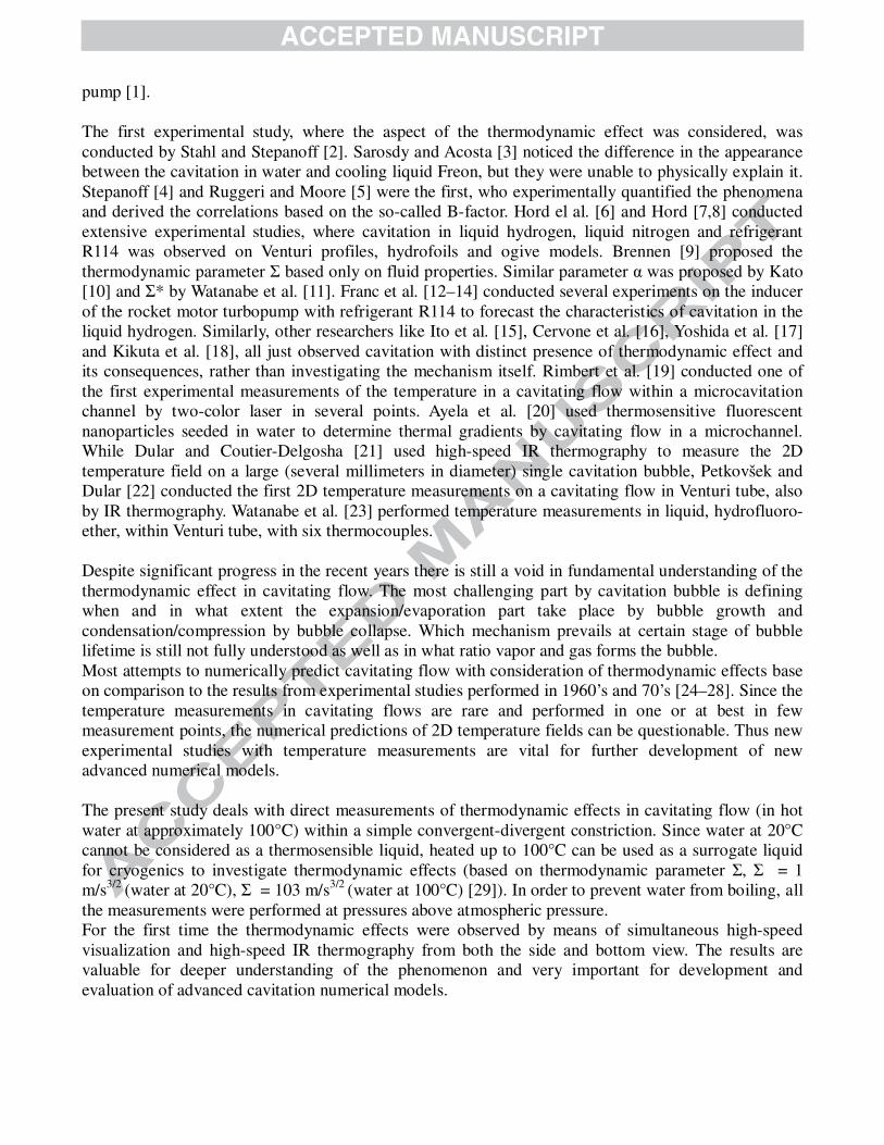
3.2 Test section Specially designed test section (Fig. 2), constructed out of transparent polycarbonate and sapphire glass, enables operation at temperatures up to 120°C. Basic geometry of the test section is a10 mm wide convergent-divergent (Venturi) constriction. The cross-section reduces with a converging angle of 18°, from initial 16×10 mm2 to 8x10 mm2 at throat position and extends back to the initial cross-section at diverging angle of 8°. The shape of the Venturi bottom, downstream from the throat, simulates an inducer blade suction side with a beveled leading edge geometry and a chord length Lref = 224 mm [35]. Side window and part of Venturi nozzle are manufactured from sapphire glass, which enables visualization by both the conventional camera and IR camera. Side window allows to observe cavitation conditions from the side view, while part of constriction (part made out of sapphire, which also serves as a window) allows the view from below, into the test section. As mentioned in section 3.1 Cavitation tunnel, a thermocouple probe J-type, with 1.5 mm in diameter, was installed 80 mm downstream of the Venturi throat into the flow (Fig. 2). The main purpose of the installed temperature sensor in the near region of the observation window is to ensure an accurate calibration procedure of the IR camera.

Figure 2: Test section

3.3 Visualization

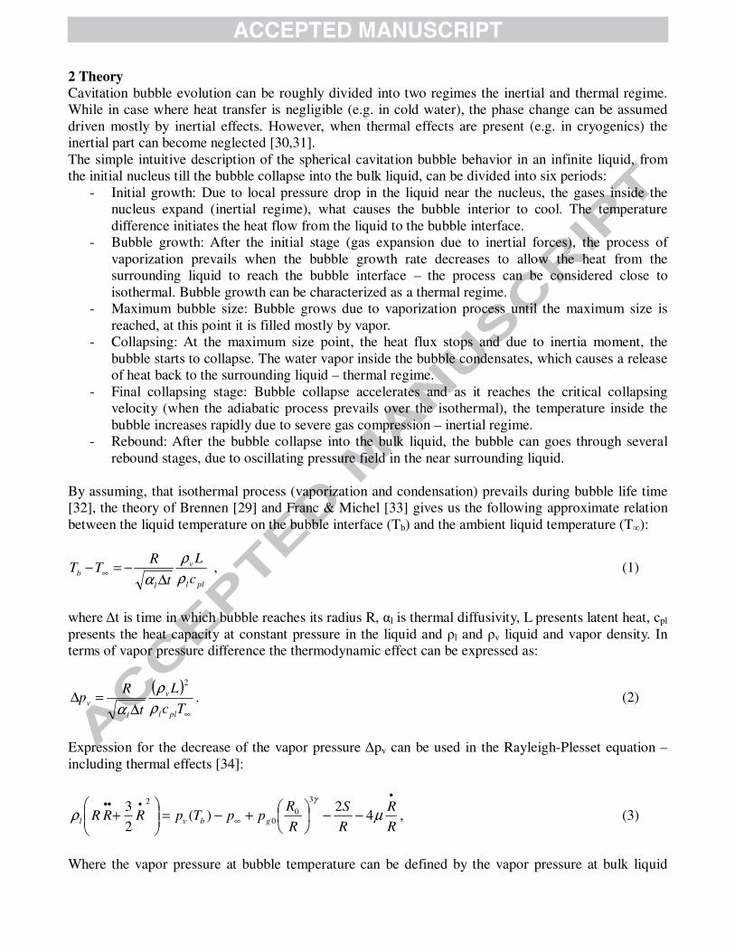
Conventional black and white high-speed camera, HiSpec4 2G mono, was used to perform visualization - to capture cavitating flow in the test section. The camera enables capturing images at 523 fps (frames per second) at 3M pixel resolution. For the present experiments frame rates of 10000 and 12000 fps at reduced resolutions (17 px/mm and 18 px/mm) were used to observe cavitating flow from side and bottom view, respectively. High-speed IR camera, CMT384SM-Thermosensorik was used for temperature measurements. The IR camera has a cooled mercury cadmium telluride detector type, with maximum resolution of 384×288 pixels and detector pitch of 20 µm. The IR camera has a spectral range between 1.5 and 5 µm and enables to adjust the integration time down to 20 µs. For the present experiments frame rates of 830 and 920 fps at a reduced resolution (10 px/mm and 8 px/mm) were set to observe temperature fields from side and bottom view, respectively. The noise equivalent temperature difference (NETD) of the IR camera is stated to be less than 20 mK for each measurement element (384×288) on the detector. To observe the cavitation phenomena, two different camera positions were set as it is shown on Fig. 3.

Figure 3: Cameras position

Setting the cameras (conventional high-speed BW camera and IR high-speed camera) in position (a) enables the observation of cavitation phenomena from the side view, while setting them in position (b) allows visualization and thermography from bottom side of the Venturi constriction. In both cases the IR camera was positioned perpendicular to the observation surface, while the conventional camera was positioned at a slight angle, which still did not deteriorate the quality of acquisition. Experimental procedure followed the following principle. The cavitation tunnel was first filled with tap water, which was then slowly heated up (time to reach 100°C was about 1 hour). During the heating process the circulation pump was operating at a minimum rotating frequency. In this time the cavitation

tunnel stayed open to ambient pressure, which allowed water to degas itself from initial 25 mg/L to approximately 5-10 mg/L (measured by Van-Slyke method at preliminary experiment). During the last minutes of the heating process, the calibration of the IR camera was performed. This was done in-situ, first at low reference temperature of 97°C and then at high reference temperature of 103°C, at elevated pressure to prevent water from boiling (all measurements were conducted inside the range of calibration-reference temperatures). When selected operating conditions (temperature, flow rate and pressure) were established, several sets of measurements (each lasting several seconds) were performed during a short time frame (about 30 minutes). If further measurements were required the camera was recalibrated to assure low uncertainty. 4 Results and discussion Experimental results are shown in respect to the viewpoint of the observation (side and bottom view into the channel flow) and to the type of data processing (mean temperature fields, standard deviation of temperatures and time resolved temperatures – temperature field dynamics). Experiments were performed at different operating conditions in order to provide sufficiently broad range of data to draw conclusions. One of the drawbacks of using the IR technique is that even a very thin layer (about 10µm) of water is opaque in the IR spectral range [36]. Consequently one can only measure the temperatures within a boundary layer (10 µm) between the sapphire window and the rest of water flow by this technique. We also tested and confirmed this by a separate series of experiments where a target was covered by a layer of water of different thicknesses and opaqueness in IR light spectrum was evaluated. The paper presents measurements at six different test conditions (Tab 1). These were chosen to give perspective from cavitation extent (E) and flow velocity (V) point of view. Table 1: Operating conditions.

Operating

point View

Q

[L/min]

p0

[kPa]

v [m/s]

throat / inlet

freestream

Re [ ]

throat / freestream σ [ ]

E 1 Side+bottom 56 180 11.7 / 5.8 353,000 / 227,000 4.8 E 2 Side+bottom 52 163 10.8 / 5.4 328,000 / 211,000 4.4 E 3 Side+bottom 46 143 9.6 / 4.8 290,000 / 186,000 3.8 V1 Side 65 172 13.5 / 6.8 409,000 / 263,000 3.1 V2 Side 87 228 18.1 / 9.1 548,000 / 352,000 3.1 V3 Side 99 263 20.6 / 10.3 624,000 / 401,000 3.1

The cavitation number σ (Eq. 7) is defined as the difference between the absolute inlet pressure p0 and vapor pressure pv (T0) divided by the dynamic pressure (ρv2/2), where velocity v presents the inlet velocity upstream the convergent part of the Venturi profile, at cross section 16×10 mm2. Cavitation number varied between 4.8 and 3.1, with the uncertainty of +/-0.05.

2

)(2

00

v

Tppv

ρσ

−= (7)

4.1 Temperature fields for various cavitation number σσσσ

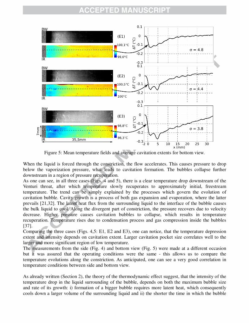
Figures 4 and 5 show the mean extends of cavitation (averaged for a period of 1 s) recorded by the BW high speed camera and the corresponding mean temperature fields recorded by the IR camera – for side (Fig. 4) and bottom (Fig. 5) views and for three cavitation extents (small – E1, middle – E2 and big – E3). In the case E1 cavitation extents over one fourth of the diverging part of Venturi, in the case E2 cavitation extents approximately over one half of the diverging part, while in the case E3 cavitation extent over the whole diverging part. For easier comparison of the data, also the temperature evolutions along the drawn dashed lines in temperature fields are shown on diagrams (on the right). The flow is from the left to the right, where position x = 0 mm corresponds to the position of the throat of the Venturi constriction. Temperature fields on figures 4 and 5 present absolute temperatures, where the absolute scale differentiates between cases, but the scale range is for all cases the same, ∆T = 0.5°C. Temperature evolutions on diagrams present temperature changes along cavitating flow, where the temperature position ∆T = 0°C corresponds to the initial freestream temperature of the each case. Freestream temperature is considered as the temperature before-upstream the Venturi throat position. Negative shift presents temperature depression below freestream temperature, while positive shift presents temperature rise.

Figure 4: Mean temperature fields and average cavitation extents for side view.

Figure 5: Mean temperature fields and average cavitation extents for bottom view.

When the liquid is forced through the constriction, the flow accelerates. This causes pressure to drop below the vaporization pressure, what leads to cavitation formation. The bubbles collapse further downstream in a region of pressure recuperation. As one can see, in all three cases (Figs. 4 and 5), there is a clear temperature drop downstream of the Venturi throat, after which temperature slowly recuperates to approximately initial, freestream temperature. The trend can be simply explained by the processes which govern the evolution of cavitation bubble. Cavity growth is a process of both gas expansion and evaporation, where the latter prevails [21,32]. The latent heat flux from the surrounding liquid to the interface of the bubble causes the bulk liquid to cool. Along the divergent part of constriction, the pressure recovers due to velocity decrease. Higher pressure causes cavitation bubbles to collapse, which results in temperature recuperation. Temperature rises due to condensation process and gas compression inside the bubbles [37]. Comparing the three cases (Figs. 4,5: E1, E2 and E3), one can notice, that the temperature depression extent and intensity depends on cavitation extent. Larger cavitation pocket size correlates well to the larger and more significant region of low temperature. The measurements from the side (Fig. 4) and bottom view (Fig. 5) were made at a different occasion but it was assured that the operating conditions were the same - this allows us to compare the temperature evolutions along the constriction. As anticipated, one can see a very good correlation in temperature conditions between side and bottom view. As already written (Section 2), the theory of the thermodynamic effect suggest, that the intensity of the temperature drop in the liquid surrounding of the bubble, depends on both the maximum bubble size and rate of its growth: i) formation of a bigger bubble requires more latent heat, which consequently cools down a larger volume of the surrounding liquid and ii) the shorter the time in which the bubble

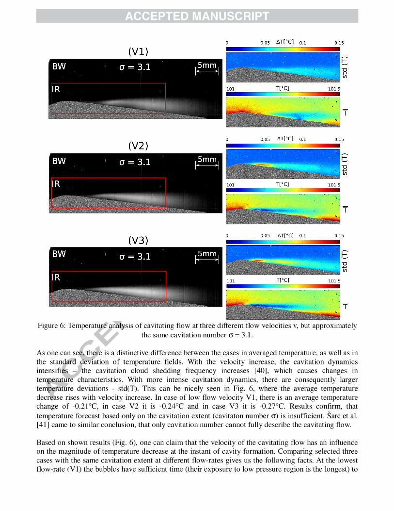
grows to its maximum size, the more intense cooling occurs in the vicinity of the bubble. Since the maximum bubble size and its growth velocity generally act contradictory (for example an increase of flowrate causes more rapid bubble growth, but they reach smaller sizes), it should be considered, that there is an optimal ratio (where the maximal cooling occurs) between these two parameters. A similar reasoning can be made for the collapse stage of bubble evolution, when the energy is released in a form of heat, which then results in a temperature rise of the nearby liquid. Based on high-speed visualization, maximum cavitation bubble size variates between few micrometers and up to millimeter. 4.2 Temperature fields for various flow velocity v The properties of the cavitating flow (the aggressiveness, dynamics, general behavior etc.) also depend on the mean velocity of the flow – even if cavitation extent is kept constant by adjusting the system pressure [38,39]. In order to investigate this for the temperature fields, we adjusted the operating conditions in a way the cavitation extent was the same for three different flowrates (Fig. 6). Average velocity, at the throat of the Venturi was v1 = 13.5 m/s, v2 = 18.1 m/s and v3 = 20.6 m/s. Consequently also the pressure conditions (evolutions) are different for the three cases (more details in Table 1). Cavitation number is for all three cases the same σ = 3.1. Left images in Fig. 6 represent the visualization of the average cavitation extent (averaged for a period of 1 s), while the diagrams on the right show mean temperature fields temperature fields – T (bottom) and standard deviation of temperature – std(T). Rectangles in the visualization images mark the area of the acquisition of the IR camera.

Figure 6: Temperature analysis of cavitating flow at three different flow velocities v, but approximately

the same cavitation number σ = 3.1.

As one can see, there is a distinctive difference between the cases in averaged temperature, as well as in the standard deviation of temperature fields. With the velocity increase, the cavitation dynamics intensifies – the cavitation cloud shedding frequency increases [40], which causes changes in temperature characteristics. With more intense cavitation dynamics, there are consequently larger temperature deviations - std(T). This can be nicely seen in Fig. 6, where the average temperature decrease rises with velocity increase. In case of low flow velocity V1, there is an average temperature change of -0.21°C, in case V2 it is -0.24°C and in case V3 it is -0.27°C. Results confirm, that temperature forecast based only on the cavitation extent (cavitaton number σ) is insufficient. Šarc et al. [41] came to similar conclusion, that only cavitation number cannot fully describe the cavitating flow. Based on shown results (Fig. 6), one can claim that the velocity of the cavitating flow has an influence on the magnitude of temperature decrease at the instant of cavity formation. Comparing selected three cases with the same cavitation extent at different flow-rates gives us the following facts. At the lowest flow-rate (V1) the bubbles have sufficient time (their exposure to low pressure region is the longest) to

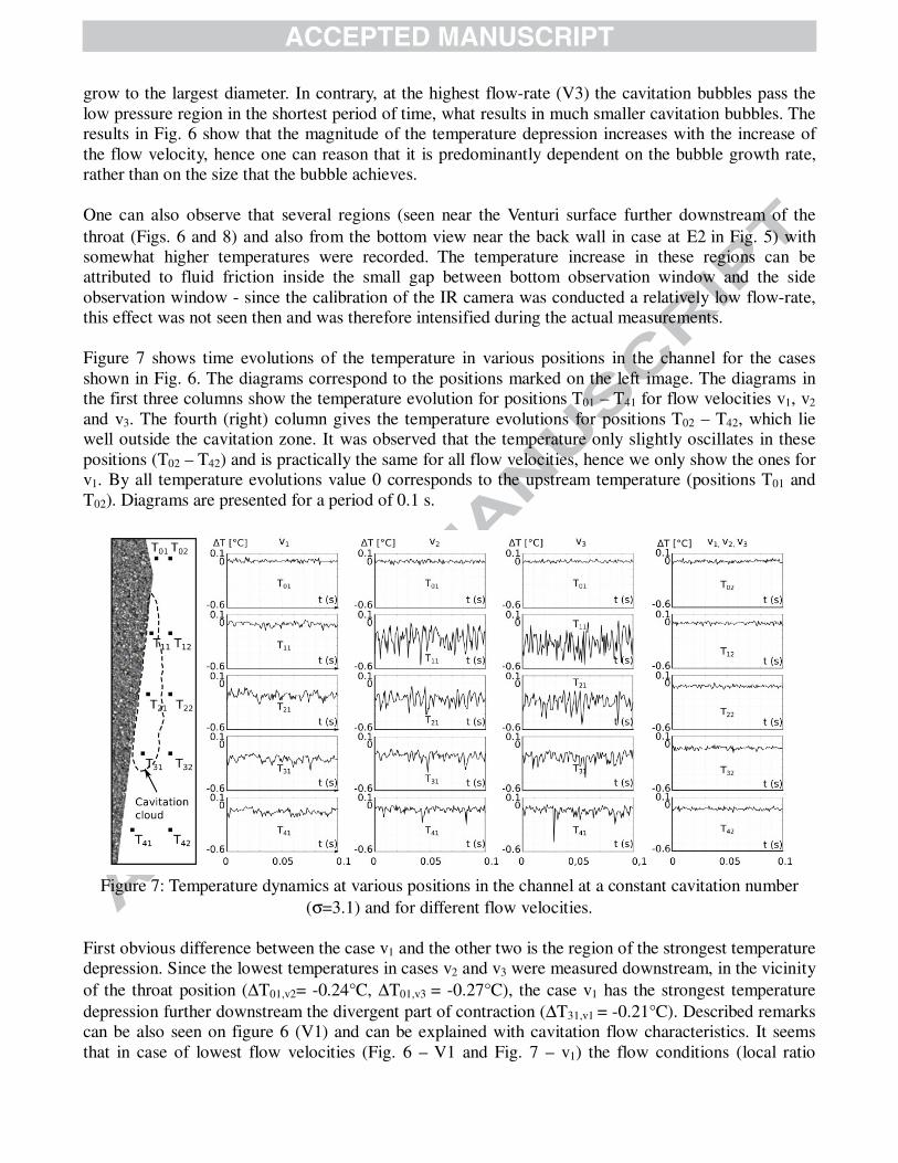
grow to the largest diameter. In contrary, at the highest flow-rate (V3) the cavitation bubbles pass the low pressure region in the shortest period of time, what results in much smaller cavitation bubbles. The results in Fig. 6 show that the magnitude of the temperature depression increases with the increase of the flow velocity, hence one can reason that it is predominantly dependent on the bubble growth rate, rather than on the size that the bubble achieves. One can also observe that several regions (seen near the Venturi surface further downstream of the throat (Figs. 6 and 8) and also from the bottom view near the back wall in case at Ε2 in Fig. 5) with somewhat higher temperatures were recorded. The temperature increase in these regions can be attributed to fluid friction inside the small gap between bottom observation window and the side observation window - since the calibration of the IR camera was conducted a relatively low flow-rate, this effect was not seen then and was therefore intensified during the actual measurements. Figure 7 shows time evolutions of the temperature in various positions in the channel for the cases shown in Fig. 6. The diagrams correspond to the positions marked on the left image. The diagrams in the first three columns show the temperature evolution for positions T01 – T41 for flow velocities v1, v2 and v3. The fourth (right) column gives the temperature evolutions for positions T02 – T42, which lie well outside the cavitation zone. It was observed that the temperature only slightly oscillates in these positions (T02 – T42) and is practically the same for all flow velocities, hence we only show the ones for v1. By all temperature evolutions value 0 corresponds to the upstream temperature (positions T01 and T02). Diagrams are presented for a period of 0.1 s.

Figure 7: Temperature dynamics at various positions in the channel at a constant cavitation number

(σ=3.1) and for different flow velocities. First obvious difference between the case v1 and the other two is the region of the strongest temperature depression. Since the lowest temperatures in cases v2 and v3 were measured downstream, in the vicinity of the throat position (∆T01,v2= -0.24°C, ∆T01,v3 = -0.27°C), the case v1 has the strongest temperature depression further downstream the divergent part of contraction (∆T31,v1 = -0.21°C). Described remarks can be also seen on figure 6 (V1) and can be explained with cavitation flow characteristics. It seems that in case of lowest flow velocities (Fig. 6 – V1 and Fig. 7 – v1) the flow conditions (local ratio

between the static and dynamic pressure in the vicinity of the throat) prevent cavitation to develop in the near region of the throat. In cases of higher velocities the pressure conditions are in favor to fully develop cavitation already at the throat vicinity, which due to evaporation process causes strong temperature depressions. As one can see, there is also a distinguish difference between the three cases (v1, v2 and v3) in temperature fluctuations (both in amplitude and frequency). Especially obvious differences are in frequencies of the temperature fluctuation, at the points (T31,v1, T11,v2, T11,v3) with strongest average temperature depression. One can see, that higher flow velocities cause more dynamic flow (more distinct cavitation cloud shedding), which leads to stronger temperature dynamics. The magnitude of the oscillations is again related to the flow velocity – the higher the velocity the larger the magnitude.

While the temperature depression for the lowest flow velocity do not strongly oscillates v131,T~∆ = ±0.05

°C, are the temperature oscillations for the other two cases distinguish stronger, v201,T~∆ = ±0.50°C and

v301,T~∆ = ±0.55°C. These values correlate well to our simple reasoning given at the end of section “2

Theory”, where the expected temperature decrease was estimated to CTTb

°−=− ∞ 6.0 .

4.3 Time resolved temperatures Figure 8 is showing simultaneous visualization of cavitation (the sequence on the left) and the recorded temperature field (the sequence on the right) for the case of the highest flow velocity (Fig. 6 - V3 and Fig. 7 - v3). The flow is from the left to the right.

Figure 8: Sequences of cavitation visualization (left) and temperature fields (right) from the side point

of view.

Cavitation in Fig. 8 is developed with strong dynamics, where the cavitation length of ¾ of the diverging part of constriction is present the whole time, with cavitation shedding on the last ¼ of the length of the constriction. Even though the re-entrant flow comes upstream, up to middle of the divergent constriction, the cavitation does not break at that point. Since the two mechanisms are known, that cause cavitation clouds to shed, re-entrant flow and reverse pressure shock wave [42], it could be a combination of both in our case. As one can see, the cavitation is at its full extent from t = 0 ms till t = 4.86 ms, when final part of the cavitation length starts to shed and collapse, what is seen on image t = 5.67, where cavitation extent gets shorten for a very small length. After this, cavitation grows back to the initial length. Interesting and obvious difference is between the seen cavitation and temperature fluctuations, since the cavitation is generally observed as steady and attached, while temperature conditions are much more dynamic. The reason for this difference is most probably in the limitation of the IR thermography, since the water is opaque in IR spectrum and parts of cavity, which do not touch the boundary layer between the observation window and water flow, cannot be detected by IR camera. As it was said before, even though the general aspect on visual cavitation is very homogeneous, its internal behavior can be much more dynamic. Figure 9 presents an interesting occurrence (recorded from a bottom point of view), where cavitation formed on a very small area in the vicinity of the Venturi throat. The flow is from the left to the right.

Figure 9: Time resolved temperature fields (bottom view).

The first bubble is seen at t=0 ms, at the same instant the temperature field is still unaffected. As the bubble grows further the liquid in the region cools down and reaches a minimum at t=3.3 ms. From this point onward the bubble is already carried downstream by the flow and it probably also moves away from the sapphire Venturi surface. Its footprint on the temperature field therefore diminishes. This

specific case is interesting as it shows that in the region, where cavitation first forms, the surrounding liquid “suffers” the temperature decrease, due to the latent heat flow. To sum up the results we investigated the interdependency between the various flow parameters (cavitation number σ, flow velocity v and cavitation intensity φ) and the magnitude of the temperature depression (Fig. 10).

Figure 10: The dependency between the cavitation number σ, flow velocity v and cavitation intensity φ and the magnitude of the temperature depression.

As already mentioned, in theory, the temperature depression depends on both the on maximal cavitation bubble size and on the time in which it reaches it. Since in the present study we did not have the possibility to determine the actual cavitation bubble size and its growth velocity, we estimated these two characteristics by three parameters. Cavitation number σ roughly describes the cavitation size and is related to the cavitation bubble, as it holds the pressure information. For a rough estimation of the cavity growth rate, we used a parameter of average velocity v in the throat of the Venturi. The third parameter, the so called cavitation intensity φ was determined by visualization images, where the brightness of the image was used as an intensity indicator. Cavitation intensity can be qualitatively related to the energy needed for cavitation generation or energy release by cavitation collapse, which can be characterized by cavitation noise or cavitation erosion. Since no audio measurements were performed or surface evaluation could be done, image characteristic brightness was used to estimate cavitation intensity. Stronger cavitation intensity can be linked to faster cavitation bubble evolution, faster bubble growth and faster bubble collapse. Cavitation intensity values base on cavitation area extents and are averaged for a period of 1 s. Values are scaled between 1 and 0, where value 1 represents the highest cavitation intensity amongst our cases and value 0 represents no cavitation present.

The upper left diagram in Fig. 10 shows the dependency between the cavitation intensity φ, which is related to both, cavity size (cavitation number σ), but also to the flow velocity v. As expected the cavitation intensity increases with decreasing cavitation number. The influence of flow velocity is not that obvious but still, higher velocity generally contributes to more intense cavitation. Stronger cavitation intensity can be linked to faster cavitation bubble evolution, faster bubble growth and bubble collapse. The upper right diagram (Fig. 10) gives the relation between the magnitude of temperature depression, cavitation number and cavitation intensity. One can see that the magnitude of the depression will be bigger for low cavitation numbers and high cavitation intensities – for cases when bubbles grow to a large size in a short period of time, what perfectly corresponds to the theory of thermodynamic effect. The lower left diagram (Fig. 10) is showing the dependency between the magnitude of temperature depression, flow velocity and cavitation number. As one can see temperature depression increases with higher flow velocity, as well as with lower cavitation number. This again confirms the reasoning based on theory. Finally the relationship between the magnitude of temperature depression, cavitation intensity and flow velocity is shown in the lower right diagram (Fig. 10). It can be seen that by increasing the intensity of cavitation also the magnitude of the temperature depression increases. On the other hand relatively poor correlation to the flow velocity is seen. This again confirms, that temperature conditions in the cavitating flow cannot be resolved by a parameter which would only include the size of cavitation or the cavitation number. 5 Conclusions The paper presents an experimental study, which has been carried out to investigate the thermodynamic effect in hot water on simple convergent-divergent constriction. Non-invasive method of temperature measurement, the high speed IR thermography, enabled us to acquire 2D temperature fields of cavitating flow, which were compared to high speed visualization images. Since even a very thin layer of water (10 µm) is opaque in IR spectrum, the measured temperature data are the temperatures of the layer between the observation window and the bulk liquid. The thermodynamic effect was observed and measured from side and bottom view perspective. The contribution of the presented work is not only valuable for the better understanding of the thermodynamic effects, but also as a set of experimental data for evaluation of advanced numerical models, which include the possibility of the presence of the thermodynamic effects in cavitating flow. The important conclusions are summarized as follows: - With 2D temperature measurements in a cavitating flow, a presence of thermodynamic effect was confirmed. In the vicinity of the forming cavities, the liquid is cooled (due to expansion and evaporation), while the temperature downstream recuperates back to the initial temperature of the liquid due to the collapse (condensation and compression) of cavities. - Experimental data confirms the theory of thermodynamic effect, which states that the magnitude of the temperature depression is dependent on the final size of the bubble and on its growth rate. - Based on the present experimental data, we were able to draw qualitative conclusions on the dependence of the magnitude of temperature depression and integral flow parameters – cavitation number, flow velocity and cavitation intensity. - Cavitation number by itself is not a sufficient parameter to describe or predict the magnitude of the temperature depression. At least one additional parameter (flow velocity or cavitation intensity) needs to be considered to estimate the thermodynamic effect. Acknowledgment The authors would like to thank the European Space Agency (ESA) for the financial support in the scope of the project “Cavitation in Thermosensible Fluids”.

References

[1] R. Sekita, A. Watanabe, K. Hirata, T. Imoto, Lessons learned from H-2 failure and enhacement of H-2A project, Acta Astronaut. 48 (2001) 431–438.

[2] H.A. Stahl, A.J. Stepanoff, Thermodynamic Aspects of Cavitation in Centrifugal Pumps, J. Basic Eng. 78 (1956) 1691–1693.

[3] L.R. Sarosdy, A.J. Acosta, Note on Observations of Cavitation in Different Fluids, ASME J. Basic Eng. 78 (1961) 1691–1693.

[4] A.J. Stepanoff, Cavitation in centrifugal pumps with liquids other than water, J. Eng. Power. 83 (1961) 79–90.

[5] R.S. Ruggeri, R.D. Moore, Method for Prediction of Pump Cavitation Performance for Various Liquids, Liquid Temperature and Rotation Speeds, NASA TN, D-5292. (1969).

[6] J. Hord, L.M. Anderson, W.J. Hall, Cavitation in liquid cryogens I - Venturi, NASA CR-2054. (1972).

[7] J. Hord, Cavitation in liquid cryogens II - Hydrofoil, in: NASA CR-2156, 1973. [8] J. Hord, Cavitation in liquid cryogens III-Ogives, NASA CR - 2242. (1973). [9] C.E. Brennen, The Dynamic Behavior and Compliance of a Stream of Cavitating Bubbles, J.

Fluids Eng. 95 (1973) 533–541. [10] H. Kato, Thermodynamic Effect on Incipient and Development of Sheet Cavitation, in: Proc. Int.

Symp. Cavitation Inception, New Orleans, LA, 1984: pp. 127–136. [11] S. Watanabe, T. Hidaka, H. Horiguchi, A. Furukawa, Y. Tsujimoto, Steady Analysis of the

Thermodynamic Effect of Partial Cavitation Using the Singularity Method, J. Fluids Eng. 129 (2007) 121.

[12] J.P. Franc, E. Janson, P. Morel, C. Rebattet, M. Riondet, Visualizations of Leading Edge Cavitation in an Inducer at Different Temperatures, in: CAV 2001 Fourth Int. Symp. Cavitation, Pasadena, CA USA, 2001: pp. 1–8.

[13] J.P. Franc, C. Rebattet, A. Coulon, An experimental investigation of thermal effects in a cavitating inducer, in: CAV 2003 Fifth Int. Symp. Cavitation, Osaka, Japan, 2003.

[14] J.P. Franc, G. Boitel, M. Riondet, E. Janson, P. Ramina, C. Rebattet, Thermodynamic Effect on a Cavitating Inducer—Part II: On-Board Measurements of Temperature Depression Within Leading Edge Cavities, J. Fluids Eng. 132 (2010).

[15] Y. Ito, K. Sawasaki, N. Tani, T. Nagasaki, T. Nagashima, A blowndown Cryogenic Cavitation Tunnel and CFD Treatment for Flow Visualization around a Foil, J. Therm. Sci. 14 (2005) 346–351.

[16] A. Cervone, E. Rapposelli, C. Bramanti, L. D’Agostino, Thermodynamic effects in hydrofoil and inducer cavitation, in: 3rd Int. Symp. Two-Phase Flow Model. Exp., Pisa, Italy, 2004.

[17] Y. Yoshida, K. Kikuta, S. Hasegawa, M. Shimagaki, T. Tokumasu, Thermodynamic Effect on a Cavitating Inducer in Liquid Nitrogen, J. Fluids Eng. 129 (2007) 273–278.

[18] K. Kikuta, N. Shimiya, T. Hashimoto, M. Shimagaki, H. Nanri, Y. Yoshida, Influence of Thermodynamic Effect on Blade Load in a Cavitating Inducer, Int. J. Rotating Mach. 2010 (2010) 1–7.

[19] N. Rimbert, G. Castanet, D. Funfschilling, Experimental Study by Two-Colors Laser-Induced-Fluorescence of the Thermodynamic Effect in Micro-Channel Cavitation, in: Proc. 8th Int. Symp. Cavitation CAV2012, Singapure, 2012: pp. 1–6.

[20] F. Ayela, M. Medrano-Muñoz, D. Amans, C. Dujardin, T. Brichart, M. Martini, et al., Experimental evidence of temperature gradients in cavitating microflows seeded with thermosensitive nanoprobes, Phys. Rev. E. 88 (2013) 43016. http://link.aps.org/doi/10.1103/PhysRevE.88.043016.

[21] M. Dular, O. Coutier-Delgosha, Thermodynamic Effects during the Growth and Collapse of a Single Cavitation Bubble, J. Fluid Mech. 736 (2013) 44–66.

[22] M. Petkovšek, M. Dular, IR measurements of the thermodynamic effects in cavitating flow, Int. J. Heat Fluid Flow. 44 (2013) 756–763.

[23] S. Watanabe, K. Enomoto, Y. Yamamoto, Y. Hara, Thermal and dissolved gas effects on cavitation in a 2-D convergent divergent nozzle flow, in: 4th Jt. US-European Fluids Eng. Summer Meet., Chicago, Illinois, USA, 2014: pp. 1–9.

[24] T. Chen, G. Wang, B. Huang, K. Wang, Numerical study of thermodynamic effects on liquid nitrogen cavitating flows, Cryogenics (Guildf). 70 (2015) 21–27. doi:10.1016/j.cryogenics.2015.04.009.

[25] C.-C. Tseng, W. Shyy, Modeling for isothermal and cryogenic cavitation, Int. J. Heat Mass Transf. 53 (2010) 513–525. doi:10.1016/j.ijheatmasstransfer.2009.09.005.

[26] Y. Utturkar, J. Wu, G. Wang, W. Shyy, Recent progress in modeling of cryogenic cavitation for liquid rocket propulsion, Prog. Aerosp. Sci. 41 (2005) 558–608. doi:10.1016/j.paerosci.2005.10.002.

[27] J. Zhu, D. Zhao, L. Xu, X. Zhang, Interactions of vortices, thermal effects and cavitation in liquid hydrogen cavitating flows, Int. J. Hydrogen Energy. 41 (2016) 614–631.

[28] J. Zhu, Y. Chen, D. Zhao, X. Zhang, Extension of the Schnerr-Sauer model for cryogenic cavitation, Eur. J. Mech. B/Fluids. 52 (2015) 1–10.

[29] C.E. Brennen, Cavitation and Bubble Dynamics, Oxford University Press, Pasadena, California, 1995.

[30] A. Prosperetti, M.S. Plesset, Vapour-bubble growth in a superheated liquid, J. Fluid Mech. 85 (1978) 349–368.

[31] L.W. Florschuetz, B.T. Chao, On the Mechanics of Vapor Bubble Collapse, J. Heat Transfer. 87 (1965) 209–220. http://dx.doi.org/10.1115/1.3689075.

[32] I. Akhatov, O. Lindau, A. Topolnikov, R. Mettin, N. Vakhitova, W. Lauterborn, Collapse and rebound of a laser-induced cavitation bubble, Phys. Fluids. 13 (2001) 2805.

[33] J.P. Franc, J.M. Michel, Fundamentals of Cavitation, Kluwer Academic Publishers, 2004. [34] M.S. Plesset, The dynamics of cavitation bubbles, J. Appl. Mech. 16 (1949) 277–282. [35] O. Coutier-Delgosha, J.L. Reboud, Y. Delannoy, Numerical simulation of the unsteady behaviour

of cavitating flows, Int. J. Numer. Methods Fluids. 42 (2003) 527–548. [36] G.M. Hale, M.R. Querry, Optical Constants of Water in the 200-nm to 200-microm Wavelength

Region., Appl. Opt. 12 (1973) 555–563. [37] B.D. Storey, A.J. Szeri, Water vapour, sonoluminescence and sonochemistry, R. Soc. Math. Phys.

Eng. Sci. 456 (2000) 1685–1709. [38] M. Dular, B. Širok, B. Stoffel, The Influence of the Gas Content of Water and the Flow Velocity

on Cavitation Erosion Aggressiveness, J. Mech. Eng. 51 (2005) 132–145. [39] M. Dular, I. Khlifa, S. Fuzier, M. Adama Maiga, O. Coutier-Delgosha, Scale effect on unsteady

cloud cavitation, Exp. Fluids. 53 (2012) 1233–1250. [40] M. Dular, R. Bachert, The issue of strouhal number definition in cavitating flow, J. Mech. Eng.

55 (2009) 666–674. [41] A. Šarc, T. Stepišnik-Perdih, M. Petkovšek, M. Dular, The issue of cavitation number value in

studies of water treatment by hydrodynamic cavitation, Ultrason. Sonochem. 34 (2017) 51–59. doi:10.1016/j.ultsonch.2016.05.020.

[42] H. Ganesh, S.A. Mäkiharju, S.L. Ceccio, Bubbly shock propagation as a mechanism for sheet-to-cloud transition of partial cavities, J. Fluid Mech. 802 (2016) 37–78. doi:10.1017/jfm.2016.425.

Figure captions:

Figure 1: Cavitation tunnel Figure 2: Test section Figure 3: Cameras position Figure 4: Mean temperature fields and average cavitation extents for side view. Figure 5: Mean temperature fields and average cavitation extents for bottom view. Figure 6: Temperature analysis of cavitating flow at three different flow velocities v, but approximately the same cavitation number σ = 3.1. Figure 7: Temperature dynamics at various positions in the channel at a constant cavitation number (σ=3.1) and for different flow velocities. Figure 8: Sequences of cavitation visualization (left) and temperature fields (right) from the side point of view. Figure 9: Time resolved temperature fields (bottom view). Figure 10: The dependency between the cavitation number σ, flow velocity v and cavitation intensity φ and the magnitude of the temperature depression.

Table captions: Table 1: Operating conditions.

HIGHLIGHTS Manuscript title: Observing the thermodynamic effect in a cavitating flow by IR thermography Research highlights:

• Direct IR measurements of the thermodynamic effects in cavitation. • Measured temperature fields in Venturi at different operating conditions. • The first temperature measurements from side and bottom view of the Venturi. • Comparison of the cavitating flow between the visualization and IR thermography. • Statistical analysis of the experimentally measured results and their evaluation.

Yours sincerely, Martin Petkovšek (corresponding author) Ljubljana, 24.10.2016 Martin Petkovšek Laboratory for Water and Turbine Machines, Faculty of Mechanical Engineering, University of Ljubljana, Askerceva 6, 1000 Ljubljana Slovenia E-mail: martin.petkovsek@fs.uni-lj.si