OCS Study BOEM 2012-074 July 2012

NORTH PACIFIC RIGHT WHALES IN THE SOUTHEASTERN BERlNG SEA: FINAL REPORT

Phillip J. Clapham, Amy S. Kennedy, Brenda K. Rone, Alex N. Zerbini, Jessica L. Crance, Catherine L. Berchok

National Marine Mammal Laboratory Alaska Fisheries Science Center

7600 Sand Point WayNE Seattle, W A 981 15

Contract Number M07RG13267 (AKC 063)

B EM BuREAU oF OcEAN ENERGY MANAGEMENT

OCS Study BOEM 2012-074 July 201 2

NORTH PACIFIC RIGHT WHALES IN THE SOUTHEASTERN BERING SEA: FINAL REPORT

Phillip J. Clapham, Amy S. Kennedy, Brenda K. Rone, Alex N. Zerbini, Jessica L. Crance, Catherine L. Berchok National Marine Mammal Laboratory Alaska Fisheries Sc ience Center 7600 Sand Point WayNE Seattle, W A 98 1 15

B EM BuREAU OF OceAN ENERGY MANAGEMENT

Study design, oversight, and funding were provided by the U.S. Department of the Interior, Bureau of Ocean Energy Management, Alaska Outer Continental Shelf Region, Anchorage, Alaska, as part of the BOEM Environmnetal Studies Program, under Contract Number M07RG 13267 (AKC 63).

This report has been reviewed by the Bureau of Ocean Energy Management and approved for publication. Approval does not signify that the contents necessarily reflect the views and policies of the Service, nor does mention of trade names or commercial products constitute endorsement or recommendation for use.

• lntroduction ................................................................................... l

• Methods ......................................................................................... 8

• Results .......................................................................................... 21

• Discussion .................................................................................... 57

• Project Summary ......................................................................... 59

• Publications and Presentations ................................................. GO

• Upcoming Publications ............................................................... 65

• Future Work ................................................................................. 74

• Acknowledgments ....................................................................... 7 4

• Dedication ..................................................................................... 75

• Literature Cited ............................................................................ 76

• Appendix A:

Peer Reviewed Publications ..................... . ...... .. .. . . .......... ..... ...... 81

• Appendix B:

Cornell Lab Passive Acoustic Monitoring Summary ............ ... ... .. .... 119

• Appendix C:

Fin Whale Preliminary Analysis ... ... ... ... .. ..... . .. ....................... .. . l33

• Appendix 0:

Foraging Ecology and Fine Scale Acoustic Studies Final Report ....... ... ........ . ............... .... .. ... 140

List of Figures

Figure 1: First high- to low-latitude match of an NPRW ................................................. 3 Figure 2: Proposed trackline for shipboard surveys during PRIEST .................................... 8 Figure 3: Systematic aerial transects in the southeastern Bering Sea in 2008 ........................ 10 Figure 4: Systematic aerial transects in the southeastern Bering Sea in 2009 ......... . ..... ... .... .. 1 0 Figure 5: SPOT 5 sate llite transmitters deployed in 2008 and 2009 ................................. .. 11 Figure 6: NPRW showing SPOT 5 satellite tags deployed on NPRW ................. .... .......... . 12 Figure 7: Sonobuoy deployment and monitoring methods: .. .......... ... ....................... .. .... 14 Figure 8: Three types of passive acoustic recorders used ...... .. .. ..... .. . ... . ........ . .. .. ..... . ... .. . 17 Figure 9: Mooring designs (not to scale) for a) M2 and M5 moorings 10.5m tall b) M4 and M8 moorings 10.5m tall c) EAR moorings 4m tall. ........................................................... 18 Figure 10: Locations of all passive acoustic recorders analyzed for this study ........ . ............ 19 Figure 11: SoundChecker analysis interface ............................................................. 20 Figure 12: Aerial (yellow) and Vessel (green) tracklines from PRIEST 2007-2011 ............... 22 Figure 13: Minke whale sightings PRIEST 2007-2011 ................................................ 23 Figure 14: Fin whale sightings PRIEST 2007-2011 .................. ... .... . . ......................... 24 Figure 15: Right whale sightings PRIEST 2007-20 II ................................................. 25 Figure 16: Humpback whale sightings PRIEST 2007-2011 ........................................... 26 Figure 17: Killer whale sightings PRIEST 2007-2011 ................ ............................. .... 27 Figure 18: Tracks ofNPRWs tagged in the SEBS in 2008 and 2009 ............................... . 30 Figure 19: Individual satellite locations of four NPRWs in the SEBS in 2008 and 2009 .. . ...... 31 Figure 20: PTT # 21803-08 shown at time of deployment, I day later, and 14 days later. ....... 32 Figure 21: Satellite transmitter attached deployed on a humpback whale in 2010 ..... ... . .. . ...... 33 Figure 22 (A-F): Individual humpback whale satellite tracks, by year. ........................ 34, 35 Figure 23: Most common right whale sounds encountered during PRIEST. ........... ............. .36 Figure 24: Location ofsonobuoys with right whale acoustic detections 2007-2011.. .... .... ...... 37 Figure 25: Location of and species detected on all sonobuoys deployed during the 2007 PRIEST survey .......................................................................................................... 38 Figure 26: Location of and species detected on all sonobuoys deployed during the 2008 PRIEST survey .. . . .. ..... ... ... . ....... .. ...... ...... ... ... .......... ............ . . ... . .. ............................... 39 Figure 27: Location of and species detected on all sonobuoys deployed during the 2009 PRIEST survey .......................... . ....... ........... ...... ...... ... ...... ......... ............................... 40 Figure 28: Location and species detected for all sonobuoys deployed during the 2010 PRIEST & CHAOZ surveys .............................................................................................. 41 Figure 29: Location of and species detected on all sonobuoys deployed during the 2011 CHAOZ survey .......................................................................................................... 42 Figure 30: Aerial sonobuoy detection results for the 2009 PRIEST survey ... ...... .. ............... .43 Figure 31: Right whale seasonal call distribution of gunshot (blue) and upsweep (red) calls on PMEL moorings 2007-2008 ... ........................ ... .. .......... .......... ........ ...... . .. .. . .. . ... . .44 Figure 32: Results from 2007-2008 Haruphone recorders superimposed on map of mooring locations ..... ............ .... .. .......... ...... . ... .. ... ................. ...................... ................ 45 Figure 33: Right whale seasonal call distribution of gunshot (blue) and upsweep (red) calls on PMEL moorings 2008-2009 ...................... ................. ........ .... .... .. . .... . .. .............. .46 Figure 34: Right whale seasonal call distribution of gunshot (blue) and upsweep (red) calls on EAR moorings 2008-2009 ................................................................................. .47

Figure 35: Results from 2008-2009 EAR and AURAL/Haruphone recorders superimposed on map of mooring locations ... ...... ....... ... ........ ... .. ....... ... ... ..... .. ..... ...... . ... ..... ..... .... .. 48 Figure 36: Right whale seasonal call distribution of gunshot (blue) and upsweep (red) calls on PMEL moorings 2009-2010 ............................................................................... .49 Figure 37: Right whale seasonal call distribution of gunshot (blue) and upsweep (red) calls on EAR moorings 2009-2010 ...... .... ...... ..... ... ...... .... .... . ...... .... ..... ... ............... .. ..... .. . 50 Figure 38: Results from 2009-2010 EAR and AURAL recorders superimposed on map of mooring locations ..... ....... ...... .... ...... .... ....... . ........ ... ... .... .............. .... ... .. ............ 51 Figure 39: Right whale seasonal call distribution of gunshot (blue) and upsweep (red) calls on PMEL moorings 2010-2011 ....... ... .......... ... ...... .... ..... . ...... .... ...... .. ....... ..... ........... 52 Figure 40: Right whale seasonal call distribution of gunshot (blue) and upsweep (red) calls on EAR moorings 20 I 0-2011 ... ...... ... ...... ..... .... .... .. . ..... ... ..... . ......... ... ...... .. .. ..... ....... 53 Figure 41: Results from 20 I 0-2011 EAR and AURAL recorders superimposed on map of mooring locations .... ..... ....... .... ........ . .......... ... ..... ... ...... .. ..... ... ........ . ...... .. ........ .. 54 Figure 42: Right whale seasonal call distribution of gunshot (blue) and upsweep (red) calls on PMEL moorings 2011 ...... .. ................... ... ..... . ........... ... ....... ... .... .... ...... .. ........ . .. 55 Figure 43: Results from 2011 AURAL recorders with map of mooring Jocations .............. .... 56

List of Tables Table l:Dates for PRIEST Aerial and Vessel Surveys ...... ........ .................... .... ........ .... 6 Table 2a:Scientist roster for PRIEST aerial surveys . ... ........ . .. ... . . . . .... .... ......... ..... ..... .... 6 Table 2b:Scientist roster for PRIEST vessel surveys ...... ...... ...... .. ........ .. .. .. .................. 7 Table 3: Numbers of sonobuoys deployed each field season .... .... ........ ........ ...... ...... ..... 15 Table 4: Recorder locations and settings .. ................ .... ......... .. .. . ........ .... ......... .. ...... 17 Table S:Vessel and aerial sightingsofmarine mammals by year .. . .. ...... ...... ......... ... . . ..... .. 21 Table 6:PRIEST Survey Effort. Includes fog, transits, and cross-legs ........ ...... ...... ...... ..... 22 Table 7:PRIEST biopsy collection summary. (Mn=humpback, Ej=NPRW, Bp=fin whale) .. ..... 28 Table 8:PRIEST NPRW sample results .. .... ......... .. ......... .. . ... ........ ..... ........... ... ........ 28 Table 9:PRIEST Individual photo ID' s, by species .... .......... .. .......... ...... ........ .... ...... ... 29 Table 1 O:NPR W Satellite telemetry metadata ...... .. ...... ..... ......... . . .. . .. ....... ...... ...... ..... 29 Table ll:Humpback whale satellite telemetry metadata .. ........ ........ .......... .... ........ ....... 33

INTRODUCTION

The North Pacific right whale (NPRW) was heavily hunted between the 1 ih and the 20th centuries, when it ceased to be the principal target of commercial whaling (Omura, 1986; Scarff, 1986, 2001 ; IWC, 2001 ; Clapham et a/., 2004 ). Protection was supposedly afforded by international treaties in the 1930s and 1940s, but the illegal harvest of hundreds of individuals by the Soviet Union, primarily in the 1960s (e.g. Doroshenko, 2000; Ivashchenko et a/., 2011, lvashchenko and Clapham, 2012) drastically impacted the recovery ofthe species.

After some debate and a failed attempt by the National Marine Fisheries Service (NMFS) to list the NPRW as a unique species, genetic work by Rosenbaum eta/ (2000) and Gaines eta/ (2005) demonstrated that the NPRW (Eubalaena japonica) is a separate species from the North Atlantic (Eubalaena glacialis) and southern (Eubalaena australis) right whales. The official species designation by NMFS was implemented in March 2008 (73 FR 12024, 06 March 2008). One month later, in accordance with the Endangered Species Act (ESA) mandates, NMFS designated a NPRW Critical Habitat (73 FR 19000, 08 April 2008) in the southeastern Bering Sea (SEBS; Figure I) , and one just south of Kodiak Island, Alaska. The location of these habitat designations was based on NPR W sighting densities after 1996 (73 FR 19000, 08 April 2008). Any activity that may affect the critical habitat (including, but not limited to, oil and gas exploration or drilling, fishing, mining, pollutant discharge, and military training) must complete an ESA Section 7 consultation through NMFS.

The existence of two discrete stocks of NPR W s has been proposed: a western population that is found in the Okhotsk Sea and in the north-western North Pacific Ocean, and an eastern population that spends the summer in the SEBS and the Gulf of Alaska (GOA) (Clapham et a/., 2004; Shelden et a/. , 2005). The eastern stock was heavily exploited by pelagic whalers beginning in 1835, and the population was seriously depleted by 1900 (Brownell eta/., 2001; Scarff, 2001 ). Sighting data from the mid-20th century suggested that a slow recovery was occurring (Brownell eta/., 2001). However, the illegal killing of 529 whales by Soviet whaling fleets in the Bering Sea and the GOA in the 1960s drove this population to near-extinction and may have compromised its long-term chances of recovery (Brownell et a/., 2001; Ivashchenko and Clapham, 2012).

Today, the eastern population of the NPRW is the most endangered stock of large whales in the world (Clapham, 1999). Recent abundance estimates based on photo-identification and genetic mark-recapture data collected during this and other projects suggest that nearly 30 individuals inhabit the southeastern Bering Sea at present, only a third of which are are females (Wade eta/., 2011).

Historical data suggest that NPRWs had an extensive offshore distribution in their feeding grounds in the BS and GOA (Townsend, 1935; Scarff, 1986; 2001 ; Clapham eta/., 2004; Shelden eta/., 2005; Ivashchenko and Clapham, 2012). Currently, the few remaining whales in the eastern stock are only a remnant of the former population, and may not fully occupy the same range they did two centuries ago (Clapham eta/. , 2004). In fact, modem sightings and acoustic detections ofNPRWs have been reported in the SEBS (Goddard and Rugh 1998; LeDuc eta/., 200 I; Tynan et a/., 2001 ; Wade et al. , 2006) and, more rarely, in the northwestern GOA (Waite eta/. , 2003; Mellinger eta/., 2004).

In 2004, Wade eta/ (2006) located a pair ofNPRWs in the BS and deployed a satellite tag on one individual. This whale was monitored for 40 days and stayed primarily on the SEBS shelf and outer shelf. During that time, a combination of telemetry tag data and acoustic

detection methods Jed to the discovery of the largest concentration of NPRW s (l 0 males and 7 females) observed since the 1960's (Wade eta/. 2006).

There is an increasing body of evidence suggesting that the SEBS middle shelf constitutes the primary habitat of NPRWs in the SEBS during the summer. Acoustic surveys (Munger et a/., 2008; Mellinger et a/., 2009; Stafford eta/., 2010) have shown that the only region in the Bering Sea where NPRWs have been consistently seen is the middle shelf (LeDuc et a/., 2001; Shelden et a/., 2005). Occasional sightings and acoustic detections have been observed in other areas (e.g. near the Pribilof Islands, National Marine Mammal Laboratory, unpublished data), but these occurrences appear rarer. This study is consistent with the existing information on NPR W occurrence in the SEBS, and underscores the theory that whales spend extended periods of time in the region. This contrasts with some acoustic evidence (e.g. Munger et a!., 2008), which suggests that NPRWs passed through the middle shelf of the SEBS intermittently and remain in the area for usually a few days.

The reasons why NPRWs concentrate in the SEBS during the summer are not yet well understood and have primarily been related to the availability and possibly high biomass of their main prey (calanoid copepods). Species of copepods upon which NPRWs feed (e.g. Calanus marshallae and Neocalanus spp.) are among the most abundant zooplankton over the Bering Sea middle shelf (Cooney and Coyle, 1982; Baumgartner eta!., unpublished data) and therefore the region appears to be a suitable habitat for these whales. However, other factors may play a role in explaining the relatively high occurrence of right whales in the SEBS middle shelf, including maternally driven site fidelity. In fact, re-sightings of photo-identified NPRWs in the SEBS have shown that some individuals regularly return to this region during their feeding season (e.g. Kennedy eta!., 2011; Wade eta!., 2011 ).

Although some information is available about the current occurrence of NPRWs in the feeding grounds, the migratory routes and wintering destinations are still unknown (Scarff, 1986; Clapham et a!., 2004). Data from historical catches and sightings indicated that a general southward movement of the population occurred in the autumn, but there are minimal records of the species anywhere in winter (Scarff 1986; Clapham et a!., 2004; lvashchenko and Clapham, 20 12). Scarff (1986) noted that there is little evidence that coastal waters of the eastern North Pacific were ever used as calving grounds by NPRWs, and therefore suggested that whales move to wintering grounds somewhere in remote offshore areas. There have been several sightings of the species between Washington, Baja and Hawaii, yet the paths used by these whales during migration and the precise geographical location of the wintering grounds have yet to be determined. Kennedy et a!. (20 11) recently reported the first high- to low-latitude (between the SEBS and Hawaii) NPRW match (Figure 1). This might suggest that Hawaiian waters represent a NPR W winter habitat, yet the Jack of consistent historical and current sightings, despite intense effort in the area, suggests that Hawaii is not the definitive migratory destination for the species.

2

170" W 160" W 150" W 140" W

Gulf of Alaska

North Pacific Ocean

1 '*,.Hawai'i

Figure 1: First high- to low-latitude match of an NPRW between Hawaii and the NPRW Critical Habitat.

50" N

40" N

30" N

20" N

Commercial hunting of other mysticetes (primarily fin and humpback whales) in the Bering Sea during the mid- to late-1990's was also extensive (Wada, 1981). Given the difficulties and expenses inherent with SEBS research (compared to more coastal areas), the region is under-sampled and the effects of those large-scale removals remain unknown. Visual line-transect surveys were conducted in the summers of 1997 (Tynan, 1999), 1999 (Moore eta/. , 2000), 2000 (Moore eta/. , 2002, BSIERP), 2002, 2008, and 2009 (Friday eta/. , in press). These surveys covered the Coastal Domain (shore to 50m), the Middle Shelf Domain (50-lOOm, includes the SEBS) and the Outer Shelf Domain (I 00-200m) (Moore et a/., 2002). Fin whales were the most numerous large whales encountered, yet sightings were clustered near the 200m contour and Pribilof Canyon. Humpbacks were commonly found along the 50m contour and north of Unimak Island. Minke whales were most often seen along the north side of the Alaskan Peninsula and along the 1OOm contour, especially near Pribilof Canyon. Only a few scattered sightings of killer whales were recorded in the SEBS. The results from these surveys depict only a broad snapshot of overall occurrence and abundance; additional sighting data from the SEBS would provide valuable knowledge to existing cetacean distribution datasets.

Through an Inter-Agency Agreement (IA) between the National Marine Mammal Laboratory (NMML) and the US Department of the Interior, Bureau of Ocean Energy Management (BOEM, formerly the Minerals Management Service, MMS), NMML conducted dedicated multi-year studies of the distribution , abundance and habitat use of North Pacific right whales in the North Aleutian Basin (NAB) and southeastern Bering Sea (SEBS). Additional funding came from the North Pacific Research Board and the National Marine Fisheries Service. This work was prompted by the need for better data to assess the potential impact of oil and gas development in the NAB area. The lA study was a multi-year project which featured multi-

3

disciplinary investigations of right whale occurrence, movements and feeding ecology. The overall goal of the lA study was to facilitate any development of future oil and gas-related mitigation (although none is being considered at present) by assessing the distribution, occurrence and habitat use of North Pacific right whales in the SEBS (North Aleutian Basin lease sale area and adjacent waters). The general objectives of the study were as follows:

• To assess distribution of NPRWs in the SEBS, with emphasis on the NPRW Critical Habitat in the Bering Sea.

• To locate whales for tagging, behavioral observations and habitat studies using ship­based visual surveys and passive acoustic methodology.

• To deploy satellite transmitters to assess movements and distribution on the feeding grounds as well as to determine migratory routes and destinations in the North Pacific Ocean.

• To deploy long-term passive acoustic recorders to assess year-round presence and relative abundance ofNPRWs in the SEBS.

• To collect photo-identification data and biopsy samples from individual whales to investigate population structure, improve estimates of abundance, determine sex, pollutant loads, diet and other studies.

The proposed study, named the Pacific Right whale Ecology STudy (PRIEST) was intended to have three yearly project field components: right whale biology (shipboard and aerial), passive acoustics, and right whale feeding and prey. Each project component is a technological discipline and was coordinated by a Project Leader with extensive experience in that discipline. All project components were conducted in the summer of 2008 and 2009. In the 2007, 2010 and 2011 field seasons, shipboard, visual and passive acoustic data were collected, but no feeding/prey or aerial surveys were conducted due to funding constraints. Table 1 illustrates the period in which field work was carried out. In all, 38 scientists from 15 different organizations participated in this project (Table 2a+b ).

Particular emphasis was placed on the deployment of satellite transmitters during this cruise. In the past decades, satellite telemetry has been used to investigate hypotheses about migratory routes and destinations. For example, Zerbini et a/. (2006a) deployed satellite transmitters on humpback whales (Megaptera novaeangliae) wintering in Brazil and demonstrated that only one of two hypothesized migratory routes to the feeding grounds in the western South Atlantic Ocean was actually used . In addition, these authors found that once whales reached the feeding areas, they stayed in areas nearly 300-500 km offshore of their historical feeding grounds. Telemetry was also used to describe the extension of movements, preferred habitat, and associations with environmental features. A study conducted with North Atlantic right whales (Eubalaena glacialis) (Mate et a/., 1997) illustrates the value of using telemetry to discover previously unknown habitats. Prior to tagging, this was considered a slow­moving species restricted to coastal areas for relatively well-defined periods of time (CeTAP (Winn & University of Rhode Island) 1982; NMFS, 1991). However, the study, conducted in the feeding grounds of the Gulf of Maine and Scotian Shelf, revealed that satellite-tagged whales were highly mobile and capable of traveling long distances (Mate eta/., 1997; Baumgartner & Mate, 2005). In addition, telemetry showed that right whales were not restricted to coastal habitats. Some individuals moved into deep waters off the continental shelf, where the species had not been previously reported (Mate eta/., 1997). This study also revealed that right whales

4

often associated with oceanographic features (warm core rings and upwelling areas), which likely concentrated prey and provided foraging opportunities.

Real-time satellite-monitoring has also been used to focus intensive research effort in areas inhabited by tracked whales, in order to collect additional data with important conservation implications. For example, locations from a satellite-monitored NPRW in 2004 were used to direct a survey vessel to locate the largest aggregation of the species recorded in the past 40 years (Wade eta/., 2006).

5

This report covers the period between March 2007 and April 2012, during which five shipboard surveys and 2 aerial surveys were conducted in the Bering Sea (Table I). In all, 38 scientists from 15 different organizations participated in this project (Table 2a+b ).

Vessel 2007 2008 2009 2010 2011

Brenda Rone

Cynthia Christman

Greg Fulling

Jeff Foster

Laura Morse

Table 1: Dates for PRIEST Aerial and Vessel Surveys.

August 29 Au ust 2 Se tember 14 Jul 16 August 30 July 30 August 23 September 3 September l 0

Table 2a: Scientist roster for PRIEST aerial surveys.

Chief Scientist, Observer, Photographer, Data Manager, Acoustician

Observer

Observer

Observer

Observer, Acoustician

6

NMML-AFSC­NOAA NMML-AFSC­NOAA Aquatic Farms Contractor Aquatic Farms Contractor NMML-AFSC­NOAA

Table 2b: Scientist roster for PRIEST vessel surveys

"

( ,c ~(· '';- ~ '"' ... , ~ .... ... '' ~· • :,,;'...:; 1'' -LL__,._ •' ,' c<~ •

Alexandre Zerbini Chief scientist, Observer, Photographer and Satellite

NMML-AFSC-NOAA Tagger

Amy Kennedy Chief scientist, Observer, Photographer, Coxswain and

NMML-AFSC-NOAA Satellite Tagger

Anthony Martinez Chief scientist, Observer, Photographer, and Coxswain SEFSC-NOAA

Billy Adams Observer, Coxswain North Slope Borough

Brenda Roue Observer, Photographer, Data Manager, Coxswain NMML-AFSC-NOAA

Carter Esch Observer, Foraging Ecology Team WHO I

Catherine Berchok Acoustician NMML-AFSC-NOAA

Dee Allen Observer, Photographer NMML-AFSC-NOAA

Desray Reeb Observer, Photographer, and Data Manager Aquatic Farms Contractor

Don Ljungblad Acoustician Marine Acoustic Consultants

Elizabeth Kusel Acoustician University of Oregon

Francesco Scattorin Acoustician Volunteer

Hans Christian Satellite Tagger Contractor

Schmidt

Heather Riley Observer, Photographer University of Alaska-Fairbanks

Holger Klinck Acoustician WHO I

James Dunn Acoustician Cornell

Jason Michalec Acoustician Cornell

Jennifer Keating Acoustician San Diego Zoo

Jessica Crance Acoustician NMML-AFSC-NOAA

Jessica Thompson Observer NMML-AFSC-NOAA

Julia Hager Acoustician University of Oregon

Karolin Klinck Acoustician University of Oregon

Lamalani Siverts Observer Volunteer

Mark Baumgartner Observer, Tagger, Foraging Ecology Team Leader WHO I

Mikkel Vellum Observer, Satellite Tagger Contractor

Jensen

Nadie Lysiak Observer, foraging ecology team WHO I

Oswaldo Vasquez Observer, biopsy sampler Atemar

Phillip Clapham Chief Scientist, Observer, Photographer NMML-AFSC-NOAA

Richard Pace Observer, coxswain NEFSC-NOAA

Sarah Mussoline Observer, foraging ecology team WHO I

Siri Hakala Acoustician Aquatic Farms Contractor

Stephanie Grassia Observer NMML-AFSC-NOAA

Suzanne Yin Observer, coxswain SWFSC

Ygor Geyer Observer, Satellite Tagger Contractor

Yulia Ivashchenko Observer, Photographer NMML-AFSC-NOAA

7

METHODS

Shipboard Surveys

Vessel surveys were conducted in the in Bering Sea during the summers of 2007 through 2011, although 2008 and 2009 were significantly longer cruises than the rest due to budget issues (Table 1 ). All surveys focused in an area on the SEBS shelf where the majority of recent (post-1970) July-September NPRWs records were reported. Initially, a survey planning area was established and zig-zag tracklines were proposed for the ship to cover the survey area (Figure 2). This design could be surveyed multiple times and could be shifted in the east-west direction in order to provide coverage of previously unsurveyed areas whenever necessary.

57' N

54' N

171 ' W

100m

200m

Pribilof Islands

BERING SEA

168' W 165' W

North Pacific Right Whale Critical Habitat in the Bering Sea

162' W

168"W 165'W 162' W 159"W

159' W

Figure 2: Proposed trackline (black) for all shipboard surveys during PRIEST. The yellow box highlights hi storically dense NPRW habitat.

57' N

54"N

Although right whales were the primary target of this project, researchers also conducted distribution, photo-ID and satellite telemetry studies on other species of large whales (namely humpback, fin and killer whales) on an opportunistic basis. Given the remote location and paucity of survey effort in the SEBS, any information on cetacean distribution and behavior in this region could contribute greatly to existing scientific knowledge. Methodology for all aspects of the project did not differ between species.

Shipboard visual survey methods were applied during daylight hours and appropriate sighting conditions (e.g. sea state below 5 in the Beaufort scale, light to no rain, > 1 mi visibility, and wind speeds below 20 knots). Visual searching was carried out by 3 observers located in the

8

flying bridge, bridge wings and/or inside the bridge. Weather perm itting, two observers were stationed outside on either side of the vessel and looked for animals with the assistance of low (7x50) and high powered (25x, ' Big Eye') binoculars. The observers scanned the water 180° in front of the vessel , from beam to beam. The recorder (who also acted as a "naked eye" observer) recorded all marine mammal sightings using the WinCruz program. When a sighting was detected, the observer would relay the following information to the recorder:

• number of reticles from the horizon to the sighting • radial angle from the trackline (bow ofthe ship) to the sighting • sighting cue (blow, animals' body, birds, etc.) • swimming direction of the group • swimming speed of the group • species identifications • best, high, and low estimates of group size

Barnett Velocispeed Crossbows (120 lb draw) with specially designed bolts and collection tips were used to collect skin and blubber samples during this project. Professional Digital Single Lens Reflex (DSLR) cameras and high quality telephoto lenses were used during PRIEST for photo-ID. During photo-ID events, 2-4 observers would photograph the target animal(s) and attempt to take high quality images of individually identifiable markings on the whales. For right whales, photographs of both sides of the callosity pattern forward of the blowholes were essential ; for humpbacks, observers focused on ventral fluke photos. At least one camera, usually the primary photographer's, would record images in RAW format but most were recorded as large jpeg files to save space. After the photo-ID events, the photographer would download and back-up their photos, then fill out data sheets that with sighting-specific meta-data and individual details for each image.

Aerial Surveys

Aerial surveys were conducted in 2008 and 2009. During 2008, the survey area was divided into three strata: Western, Central and Eastern (Figure 3). The Central stratum included the NAB lease area and the region where a majority of the right whale records (sightings, acoustic detections and satellite telemetry locations) had been documented since the late 1960s. Due to the lack of sightings in 2007, effort was also applied in the Western and Eastern strata. Transect lines consisted of a north-south and east-west grid pattern, producing equal probability of detection in all three strata. In 2009, the survey was redesigned to account for the limited range of the right whales observed in 2008 within the Critical Habitat; tracklines were designed with fine-scale coverage to account for the limited visibility conditions often encountered in the Bering Sea (Figure 4). Survey design consisted of 30 boxes. Each box contained nine north­south transect lines, 40 nm in length with 5 nm spacing between tracklines. Survey boxes were designed to cover the entire Critical Habitat and the NAB and immediate surrounding waters. The small-scale design proved more effective in locating individual animals given that the right whales in 2008 were only observed in singles or pairs.

During both years, the survey team consisted of two observers and a data recorder/observer (and acoustician in 2009). Sighting data was collected by a team of three scientists using standard line-transect methods. One scientist was designated as data recorder for the entire survey project to maintain consistency. The aircraft was flown at a speed of 110 knots.

9

Surveys were flown at altitudes ranging from 600-1000 ft, weather permitting. Surveys lasted between 4 and 6 hours, depending on the location of the survey area to the refueling destination. If conditions permitted, the aircraft would refuel and conduct a second survey in a given day.

55' N

170'"W' 168"W 166"W 164"W 162"W 160"W

~ ,k_ ~r

65 Ell 260 ~lometers

168"W 166"W 164"W 162W 160"W 158"W

Figure 3. Systematic aerial transects in the southeastern Bering Sea in 2008.

170~ 185'W

16 21

• • JIJiy

Allgutt

~--~~--~ri---~~~~'~-M~~--~~ · ~ Oclobe<

Riglll- s.gtmgs 200e

. 0 2~ :10

~ irb -'----!.!!or-'--',~oo...-'-' _..__.___,

185W 180-w'

Figure 4. Systematic aerial transects in the southeastern Bering Sea in 2009.

10

4'N

Satellite Telemetry

Once right whales or other target species were seen by vessel observers, inflatable boats were launched for tag deployment whenever possible. Satellite transmitters were attached to the body ofNPRWs and humpback whales using the Air Rocket Transmitter System (ARTS, Heide­J0rgensen et al., 2001), which is a modified marine safety pneumatic line thrower. Tagging took place at distances from 6-1 Om. Tag deployment in previous right whale tagging studies (Mate et al., 1997; Wade et al., 2006) was conducted with a pole (see Heide-J0rgensen et al., 2003) and required a closer approach (within 3-6m) to the whales. The use of the ARTS allowed tag deployment from greater distances and therefore provided more tagging opportunities.

All species were tagged with the implantable configuration of the SPOT 5 transmitters produced by Wildlife Computers (Redmond, WA) (Figure 5). These instruments are cylindrical in shape and contain an ARGOS satellite PTT. The tags are divided into two components. The transmitter cylinder is a stainless steel tube where the electronic components of the tag are cast. It measures 11.5 em in length and 2 em in diameter. The cylinder is attached to the anchoring system, which corresponds to a 15-20cm long stainless steel rod of smaller diameter (0.8 em) with 3-5cm retention flanges (or barbs) at the proximal end. When deployed, approximately 4 em of the tag remains external to the body of the whale, with an antenna extending out of the distal end of the tag (Figure 6). Attempts were made to photograph and biopsy sample all tagged whales for individual identification and sex determination. Tag deployment, photo-identification and biopsy sampling were performed according to regulations and restrictions specified in the existing permits issued by the NMFS to the National Marine Mammal Laboratory (permit #782-1719-09 14245

Figure 5: SPOT 5 satellite transmitters deployed on NPRWs in the SEBS in 2008 and 2009.

11

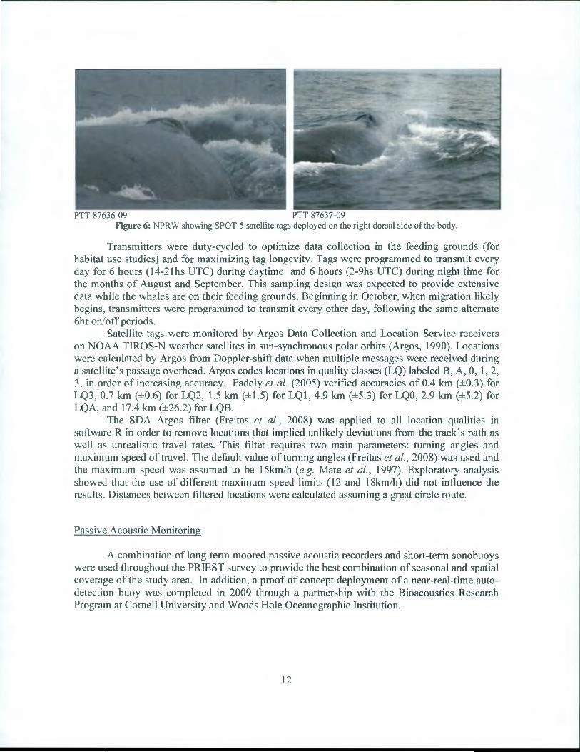
Figure 6: NPRW showing SPOT 5 satellite tags deployed on the right dorsal side of the body.

Transmitters were duty-cycled to optimize data collection in the feeding grounds (for habitat use studies) and for maximizing tag longevity. Tags were programmed to transmit every day for 6 hours (14-2lhs UTC) during daytime and 6 hours (2-9hs UTC) during night time for the months of August and September. This sampling design was expected to provide extensive data while the whales are on their feeding grounds. Beginning in October, when migration likely begins, transmitters were programmed to transmit every other day, following the same alternate 6hr on/off periods.

Satellite tags were monitored by Argos Data Collection and Location Service receivers on NOAA TIROS-N weather satellites in sun-synchronous polar orbits (Argos, 1990). Locations were calculated by Argos from Doppler-shift data when multiple messages were received during a satellite's passage overhead. Argos codes locations in quality classes (LQ) labeled B, A, 0, I, 2, 3, in order of increasing accuracy. Fadely eta/. (2005) verified accuracies of 0.4 km (±0.3) for LQ3, 0.7 km (±0.6) for LQ2, 1.5 km (±1.5) for LQI, 4.9 km (±5.3) for LQO, 2.9 km (±5.2) for LQA, and 17.4 km (±26.2) for LQB.

The SDA Argos filter (Freitas et a/., 2008) was applied to all location qualities in software R in order to remove locations that implied unlikely deviations from the track's path as well as unrealistic travel rates. This filter requires two main parameters: turning angles and maximum speed oftravel. The default value of turning angles (Freitas eta/., 2008) was used and the maximum speed was assumed to be l5km/h (e.g. Mate et a/., 1997). Exploratory analysis showed that the use of different maximum speed limits (12 and l8km/h) did not influence the results. Distances between filtered locations were calculated assuming a great circle route.

Passive Acoustic Monitoring

A combination of long-term moored passive acoustic recorders and short-term sonobuoys were used throughout the PRIEST survey to provide the best combination of seasonal and spatial coverage of the study area. ln addition, a proof-of-concept deployment of a near-real-time auto­detection buoy was completed in 2009 through a partnership with the Bioacoustics Research Program at Cornell University and Woods Hole Oceanographic Institution.

12

Sonobuoys

Sonobuoys played a key role in locating right whales during the field surveys. They had been used successfully in a previous tagging study (Wade et al., 2006) to locate individual whales, and were invaluable during PRIEST. Sonobuoys would routinely detect calling right whales up to 10 nm away, even when visual observations were limited by darkness, high sea states, or fog (as was often the case in the Bering Sea).

Designed for military purposes, sonobuoys (Figure 7a) are free-floating, expendable, short-term hydrophones that transmit signals in real time via VHF radio waves to a receiver on a vessel (or aircraft). Because they contain batteries, sonobuoys have a limited shelf life. The military is often unable to use all of their sonobuoys before the expiration date passes. Because their operations have no room for equipment failure, expired sonobuoys are sent to surplus, where many are donated to marine mammal research projects, like this one, for passive acoustic research.

The functional range of sonobuoys is dependent on two factors. The distance a transmitting sonobuoy can be detected by the antenna on the vessel (or aircraft), or the in-air reception range, depends on the transmission power of the sonobuoy (battery strength dependent), the height, type, and gain of the antenna, and whether any objects block the line of sight between the two (such as ocean waves or superstructure on the ship). An omnidirectional antenna was installed in all years of the survey; starting in 2010 a Yagi directional antenna was also installed. Both antennas were placed up in the crow's nest ofthe vessel (Figure 7b) with the directional antenna facing astern. The Yagi was used primarily during transit when the sonobuoy was guaranteed to be behind the vessel, and the omnidirectional antenna was used for monitoring multiple sonobuoys simultaneously. A switch located in the bridge was used to select which , antenna fed into the monitoring system. The omnidirectional antenna had a maximum in-air reception range of approximately 8-10 nm. The Yagi antenna almost doubled the in-air reception range, providing 15 miles or more on some buoys. The distance a calling animal could be detected by the sonobuoy hydrophone, or acoustic detection range, is highly dependent on oceanographic conditions, but typically averages 1 0-15nm.

13

B Omnl .........

Figure 7: Sonobuoy deployment and monitoring methods: a) A sonobuoy is deployed off the rail of the vessel. It transmits up to b) one of two receiving antennas located on the crow's nest. c) Specialized receiving equipment located on the bridge is used to record and monitor the sonobuoy acoustic signal, d) DifarTracker software screenshot.

Sonobuoys come in two main types: omni-directional sonobuoys can record up to 100 kHz, a frequency range that includes most marine mammal vocalizations. DiF AR (Directional Frequency Analysis and Recording) sonobuoys can record up to 2.5 kHz, which is still sufficient for most vocalizations, but transmit directional bearing information in addition to the acoustic signals. By deploying two or more DiFAR sonobuoys a few miles apart, we can obtain a cross­fix or triangulation on a calling whale and localize on the whale's position in real-time (detailed below). This information can be used to verify that the calling animal is the same as the one spotted by the observers, to conduct focal follows that correlate acoustic behavior with visual behaviors, or most importantly - to help direct the vessel to the calling animal so that visual observations can be made, photographs and biopsy samples can be taken, and telemetry tags can be attached.

The sonobuoys were removed from their housing on the deck of the ship and were stationed alongside the rail of the ship nearest the bridge for easy deployment. When removing the buoys from the housing and prepping them for deployment, all excess or unnecessary plastic or parts were removed to reduce the amount of marine debris going into the sea. On some sonobuoy models, the minimum depth of deployment was greater than the depth of the water column. To shorten the deployment depth, modifications were made to the sonobuoys, including taping up additional sensor arrays, cutting off excess string, and tying up the top portion of the buoy containing the coiled cable to prevent accidental deployment. After such modifications were completed, the approximate deployment depth of the sonobuoys was 70ft. Sonobuoys were deployed every year of the right whale survey (2007 -201 0) and continue to be deployed during the transit legs for the CHAOZ (Chukchi Acoustic Oceanographic and Zooplankton) survey which pass between Dutch Harbor and Nome, AK. Since 2007, nearly

14

1000 sonobuoys (with an overall success rate of 79.9%) were deployed for this study (Table 3). Locations of all successfully deployed sonobuoys can be found in Figures 23-27 in the Results section.

Sonobuoys were also used in 2009 from the aerial survey platform (See Rone eta/, 2011 for aerial sonobuoy methods). Because the sonobuoys used by the boat and the plane were the same, monitoring was conducted by both observation platforms whenever either were in range of a deployed sonobuoy.

Table 3: Numbers of sonobuoys deployed each field season: #successful (total #).

Sonobuoy type 2007 2008 2009 2010 2011

DiFAR 79 (133) 2.26 (2.90) 2.61 (305) 89 (100) 118 (141)

Magnavox 578 Omni 0 11 (12) 3 (4) 2 {2) 1 (1)

TOTAL 79 (133) 237 (302) 264(309) 91(102) 119(142)

Analysis of sonobuoy data was undertaken primarily in real time during the cruise. The acoustic output from the antenna was fed into 3 WiNRADiO G39WSBe receivers (Oakleigh, Australia). The digital output of these receivers were input through a MOTU model UltraLite mk3 external soundcard (S & S Research, Inc., Norwood, MA) to the laptop computer (Figure 7c). Two windows of the sound analysis program, Ishmael 1

, were used to simultaneously save the sound files to an external drive as well as to monitor the recordings. An acoustic technician monitored the scrolling spectrograms of the recordings from each sonobuoy aurally as well as visually, and noted the species detected during its deployment. Monitoring occurred in real time 24/7 throughout the cruise, although sonobuoys were deployed only every three hours while transiting.

When a call of interest was detected, a box was drawn around it and a custom designed tracking program, DifarTracker (Figure 7d), was launched. DifarTracker was written in-house using Matlab, the demultiplexing software created by Greeneridge Sciences, Inc. (Santa Barbara, CA), and the Ishmael-to-Matlab demultiplexer interface written by Mark McDonald (Whale Acoustics, Bellvue, CO). DifarTracker produces a map of sonobuoy deployment locations and the vessel track (updated every minute). After the call is processed, a line indicating the bearing angle from the sonobuoy is drawn on the map. When the call is detected on multiple sonobuoys, DifarTracker calculates a cross-fix position (latitude/longitude) from the intersection of two of the bearing angle lines. On occasion, a sonobuoy with shifted bearing information was encountered. Since DifarTracker produces a track of the vessel, the bearing angle to the ship can be calculated and compared to the actual ship position to calibrate the bearing angle from the DiFAR recording, eliminating this bearing error. Once NPRW calls were detected and their position was calculated, the ship was then diverted towards the calls to locate the whale(s) or start an expanding box search from that location.

1 Mellinger, David K. , 2001 . Ishmael 1.0 User's Guide. NOAA Technical Memorandum OAR PM EL-120, available from

NOANPMEL, 7600 Sand Point WayNE, Seattle, WA 98115-6349

15

Aerial Acoustics

After taking into consideration the limitations that were encountered on the 2008 aerial survey (i.e. limited visibility and high sea states combined with minimal numbers of right whales), an acoustic component was incorporated into the aerial survey this year in order to maximize the detection probability and expand coverage. (See Appendix A, pg. 99 for further details)

Long-term moored acoustic recorders

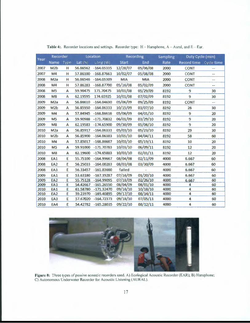
While sonobuoys provide real-time monitoring capabilities with broad spatial coverage, they are limited to only the time period of the cruise. To obtain a full picture of the seasonal distribution of the right whales, long-term moored passive acoustic recorders were used. Three different types of passive acoustic recorders (Figure 8) were deployed on two different types of sub-surface moorings (Figure 9).

Every year since 2006, through the generosity of Dr. Phyllis Stabeno (Pacific Marine Environmental Laboratory (PMEL/NOAA)), NMML has been able to occupy four (M2, M4, M5, and M8, Figure 1 0) of her long-term oceanographic moorings located along the 70 m isobaths in the Bering Sea. The 2006 and 2007 recorders were funded by a North Pacific Research Board project (data graciously provided by Drs. Kate Stafford (APL!UW) and David K. Mellinger (PMEL/Oregon State University)), and were picked up by the PRIEST survey in 2008. No ship time or mooring costs were ever incurred by the PRIEST survey for any of these deployments. This report includes results from 2007-2011. Two types of passive acoustic recorders have been deployed on these PMEL moorings. Haruphones (Haru Matsumoto, CIMRS/NOAA, Newport, OR) were deployed on the M2 and M4 moorings during both the 2007-2008 and 2008-2009 deployments, and AURALs (Autonomous Underwater Recorder for Acoustic Listening, Multi-Electronique, Inc., Rimouski, QC) were used on the M5 and M8 moorings during the 2008-2009 deployments, and on all four moorings from 2009 on. Acoustic Doppler Current Profilers are collocated on all PMEL moorings (Figures 9a and 9b) while Acoustic Water Column Profilers (for zooplankton and fish) are located underneath the AURALs on the M2 and M4 moorings (Figure 9b ). Information on the recording period, sampling rate, and duty cycle can be found in Table 4.

16

Table 4: . Recorder locations and settings. Recorder type: H - Haruphone, A - Aural, and E - Ear.

Recorder location Recording Sampling Duty Cycle (min) Year

Name Type lat (N} long (W} Start End Rate Record time Cycle time

2007 M2b H 56.86562 -164.05335 12/28/07 05/06/08 2000 CONT --

2007 M4 H 57.86100 -168.87663 10/02/07 05/08/08 2000 CONT --2008 M2a H 56.86546 -164.05309 MIA MIA 2000 CONT --

2008 M4 H 57.86283 -168.87700 05/16/08 05/02/09 2000 CONT --

2008 M5 A 59.90475 171.70475 10/01/08 05/29/09 8192 9 30

2008 M8 A 62.19595 174.65925 10/01/08 07/02/09 8192 9 30

2009 M2a A 56.86610 -164.04630 05/06/09 09/25/09 8192 CONT --

2009 M2b A 56.85950 -164.06333 10/15/09 03/07/10 8192 26 30

2009 M4 A 57.84945 -168.86616 05/06/09 04/01/10 8192 9 20

2009 M5 A 59.90988 -171.70832 06/01/09 03/29/10 8192 9 20

2009 M8 A 62.19583 -174.65900 09/30/09 05/06/10 8192 9 20

2010 M2a A 56.85917 -164.06333 05/03/10 05/23/10 8192 29 30

2010 M2b A 56.85900 -164.06383 10/05/10 04/04/11 8192 58 60

2010 M4 A 57.85017 -168.86667 10/03/10 05/19/11 8192 10 20

2010 M5 A 59.91000 -171.70783 10/03/10 06/09/11 8192 12 20

2010 M8 A 62.19600 -174.65883 10/03/10 02/01/11 8192 12 20

2008 EA1 E 55.75100 -164.99667 08/04/08 02/11/09 4000 6.667 60

2008 EA2 E 56.25033 -164.00283 08/03/08 03/30/09 4000 6.667 60

2008 EA3 E 56.33457 -161.83660 fa il ed - 4000 6.667 60

2009 EA1 E 53.63180 -167.39287 07/16/09 01/20/10 4000 6.667 60 2009 EA2 E 55.75128 -164.99095 07/18/09 02/26/10 4000 6.667 60 2009 EA3 E 54.42667 -165.26550 08/04/09 08/01/10 4000 4 60 2010 EA1 E 61.58780 -171.32470 09/16/10 10/18/10 4000 4 60 2010 EA2 E 59.23970 -169.40895 09/17/10 08/14/11 4000 4 60 2010 EA3 E 57.67020 -164.72373 09/18/10 07/05/11 4000 4 60

2010 EA4 E 54.42782 -165.28035 09/22/10 08/12/11 4000 4 60

Figure 8: Three types of passive acoustic recorders used. A) Ecological Acoustic Recorder (EAR); B) Haruphone; C) Autonomous Underwater Recorder for Acoustic Listening (AURAL).

17

A

:n .­==

.,... 8

=--

==-- -

c

Figure 9: Mooring designs (not to scale) for a) M2 and M5 moorings 10.5m tall b) M4 and M8 moorings 10.5m tall c) EA R moorings 4m tall.

Starting in 2008, EARs (Ecological Acoustic Recorders, in collaboration with Drs. Marc Lammers and Whitlow Au, Hawaii Institute ofMarine Biology, Univ. ofHI, Kaneohe, HI) were also deployed on NMML-owned sub-surface moorings (Figure 9c) in various locations throughout the Bering Sea (EA1- EA4, Figure 10). Information on the recording period, sampling rate, and duty cycle for these EARs can be found in Table 4.

Although the last field season of the PRIEST survey was in 2010, because the cost of redeploying these recorders is minimal and because of the importance of maintaining a long time record of data for this area, we have continued to deploy these recorders during our transit legs through the Bering Sea for the CHAOZ (Chukchi Sea Acoustics, Oceanography, and Zooplankton) study.

Data from these long-term recorders were analyzed separately for right whale gunshot and upsweep calls, because these two call types span different frequency bands. The data were also analyzed for fin whale calls, results of which can be found in Appendix C.

Analysis of the data from these long-term recorders was carried out with a Mat lab-based sound analysis software package, SoundChecker, developed in-house. SoundChecker was designed in response to the sheer magnitude of passive acoustic data recordings that need to be analyzed, the enormous overlap of the acoustic repertoires of many Alaskan marine mammal species, and the lack of any semblance of a stereotyped call for most of the species. We began analysis in 2009 using autodetectors, but spot-checks of those results showed that these auto­detectors were missing many of the right whale calls. In fact, comparison of the autodetector results with the current results shown in this report confirms this. Since this species is critically endangered, we found it safer to process the data by hand rather than risk missing any right whale detections.

18

Figure 10: Locations of all passive acoustic recorders analyzed for this study. A) 2008, B) 2009, C) 20 I 0, D) 201 I .

In addition, 2007 data from the M2 and M4 moorings were also analyzed.

The trouble with any spectrogram based sound analysis program is the amount of computational time needed to generate the spectrograms. This time increases as the frequency band of interest increases. SoundChecker (Figure 11) operates on image files (Portable Network Graphics (PNG) format) that can be generated ahead of time, so no time is wasted waiting for the spectrogram to be generated during the analysis sessions. For each image file the analyst decides if a species or call type is present, and selects the appropriate Yes/No/Maybe button. If No or Maybe is selected the program jumps to the next image file. If Yes is selected, then the program skips ahead to the first image file of the next time interval. An analysis interval of three hours is used for the AURALs and Haruphones, while every image file was reviewed for the EARs. Since many sounds are difficult to determine visually, there are playback and zoom options available to the analyst.

19

PlAY 5X

PLAY _x

~ 200

~ 100 LL

~ 200

~ 100 LL

0

'N 200 ~

~ 100 LL.

rV"tupsweep.al:al:3h:.99- 294

AU-8S02a-11 0522-053500-30ed801 5s

10 20 30 40 50 60 70

ZOOM

80 90 100 110 120 130 140 150

I• \ \ ' 1 ol \ ,

1

' \. ·~ , ll ., 11 '1 '1 1 ~ ~

I ~~.. " , r • ;

i .. ~... I .... ~. , I M<". . ' ' ... . •• 1 ,' ~ ~ ,.· . ' ' ~.:~ .iJ.~.:,':~ I ,.---.,_ ·~·-+'~"'-.,.._-hc••-::lf>"'4~~ ·~...,.,....,__.-,,-~~~--~~ • __.,_ "'·- __..--.,~

• 160 170 180 190 200 21 0 220

230 240 250 260 270 280 290 300 Time (sec)

Figure 11: SoundChecker analysis interface. Spectrogram shown is for the Bering Sea PMEL M2 mooring deployed in 2011 and represents 300 s of recordings starting at 05:35:00 UTC on 22 May 2011. The upper information bar shows that this analyst is looking for right whale upsweep calls in 3 hour analysis intervals and is 294 spectrograms into their analysis session. Present are humpback and fin whale calls. SoundChecker was written in the Matlab programming language.

Near-real-time auto-detection buoy

A Right Whale Detection System (AB-22) built by Cornell University's Bioacoustics Research Laboratory (BRP) and Woods Hole Oceanographic Institution (WHOI) was deployed at 57°08.64'N and 164° 30.54'W. The system is a demonstration passive acoustic monitoring system that utilizes an automatic detection buoy with the capability to detect and notify (via an iridium link) a land-based station of the occurrence of North Pacific right whales in the vicinity of the buoy. The buoy was paid for by the Bureau of Ocean Energy Management (BOEM) funded Chukchi Acoustics, Oceanography, and Zooplankton (CHAOZ) study, as proof of concept needed to be determined prior to its deployment in the Chukchi Sea for that project. The land-based station then notified both the survey ship and airplane via a twice daily text message. The system was deployed from the USCGC Healy on July 20, 2009. This buoy remained in the water for just over one month, and recovery of the buoy occurred on 22 August 2009 from the NOAA ship Oscar Dyson. In addition, an acoustic pop-up buoy from Cornell was recovered on

20

the same day less than half a mile from the automatic detection buoy. See Appendix B for the full Cornell report.

RESULTS

Shipboard and Aerial Surveys

Humpback whales were by far the most prevalent species observed (Figure 16), but several other species of large and small cetaceans were also observed (Table 5, Figures 13-17). A total of 13,605nm of combined aerial and shipboard effort were surveyed (Table 6, Figure 12).

There were 79 sightings of 120 individual right whales (Figure 14); this number reflects the high resighting rate of individual right whales during the study. All right whale sightings were photo-ID'd and only 12 individuals were identified during this study. Although right whales were acoustically detected during both the 201 0 and 20 11 surveys, inclement weather directly impacted observational work, thereby significantly reducing effort when compared to previous years (Table 6); the lack of visual sightings are the result of consistently poor visibility and weather conditions, not absence of aerial survey support. High seas and poor visibility would have likely restricted aerial survey operations.

Table 5: Vessel and aerial sightings/(number of animals) of marine mammals by year, PRJ EST data only .

VESSEL AERIAL

SPECIES 2007 2008 2009 2010 2011 2008 2009 Total

Right* 0 22(37) 24(43) 0 O* 10(12) 23(28) 79(120)**

Humpback 60(349) 50(107) 36(137) 38{82) 54(122) 129(262) 17(29) 384(1088)

Fin 43(71) 28(47) 107(190) 2(6) 2(2) 40(91) 84(156) 17(563)

Minke 3(3) 7(9) 1(1) 4(5) 2(2) 0 0 17(20)

Gray 0 0 0 0 5(7) 0 0 5(7)

Sei 0 0 0 0 0 2(4) 0 2(4)

Killer 16(120) 14(61) 7{46) 2(12) 3(12) 4(27) 0 46(278)

Unid Beaked 0 0 0 0 0 2(4) 0 2(4)

Pacific white-sides 0 0 0 0 0 4(92) 0 4(92)

Dall's porpoise 38{216) 0 0 8(50) 2(19) 7(47) 0 55(332)

Harbor porpoise 12(20) 0 0 17(27) 21(31) 15(21) 0 65(99)

*One NPRW was seen in 20 II during the CHAOZ cruise, but those data are not included here. **Due to the extremely high resighting rate of North Pacific right whales, these numbers do not reflect the number of individuals seen per season. Only 12 individual right whales were identified over the course of this study.

21

I

' I

Table 6: PRIEST Survey Effort. Includes fog, transits, and cross-legs.

EFFORT

Year

2007

2008

2009

2010

2011

Bering Sea

' '\.s~ Matthews .'-., Island

I

/

(

J

Platform

Vessel

Vessel

Aerial

Vessel

Aerial

Vessel

Vessel

Nunivak Island

I

I

On Effort (nm)

1806

1206

6292

1013

2590

416

282

13605

North Pacific Ocean

Aerial Tr ck Vessel Track

Figure 12: Aerial (yellow) and Vessel (green) track lines from PRIEST 2007-20 II

22

ltoom

"""" -. e I

Pribilof Islands

Minke W~~~ Sightings 20 \ 011

- 50m

/ I I

Bering Sea

.... ""'"

Figure 13: Minke whale sightings PRI EST 2007-201 I.

23

e Vessel Sightings

"

..

,.

100m

<::;::>'

Fin Whale Sightings 20'07-2011

SOm

t ~ i:k>l .... I

nds •

• • Bering ea

Figure 14: Fin whale sightings PRIEST 2007-2011.

24

Alaska

<> Efts~ I

Ba l

100m

..

Pribilof Islands

. ~

Bering Sea

Right ~ale Sightings 20~·2011

50m

"''WW

-erlstpl Bay (

* Vessel Sightings

Figure 15: Right whale sightings PRIEST 2007-2011.

25

100m

9"

Humpback Whale Sightings 2007-2011

SOm

... Pnbtlof ... Islands

'> ...

Bering Sea

\ )

.& Vessel Sightings

Figure 16: Humpback whale sightings PRJ EST 2007-2011.

26

100m

" Pnbilol

' Islands

~ '

Bering Sea

Killer W~~e Sightings 200{'·2011

50m

Figure 17: Killer whale sightings PRIEST 2007-2011

27

tfrlstpl Bayc t

/

Biopsy Samplin g:

In total, 4 right whales, 21 humpbacks and 5 fin whales (with one duplicate) were sampled (Tables 7 and 8) .

Table 7: PRJ EST biopsy co llection summary. (Mn=humpback, Ej =NPRW, Bp=fin whale)

biopsy Date species sgt wh reaction gen arc oth Notes # # # h 001 8/11/2007 Mn 158 1 y y y ES, tag 1, bio 1

002 8/11/2007 Mn 158 1 y y y MO, bio2

003 8/11/2007 Mn 158 3 y y y ES, tag2 , bio 3

004 8/11/2007 Mn 158 1 y y y SN, bio4

005 8/22/2007 Mn 242 3 y y y Bio1

006 8/23/2007 Mn 315 1 y y y bio 1 sgt 315-1

007 8/23/2007 Mn 315 1 y y y bio2 subgp6

008 8/23/2007 Mn 315 1 y y y bio3 subgp9

009 8/23/2007 Mn 315 1 y y y bio4 subgp1 0

010 8/23/2007 Mn 315 1 y y y bio5 subgp12 011 8/23/2007 Mn 315 1 y y y bio6 subgp14 012 8/23/2007 Mn 315 1 y y y bio7 subgp15 013 8/23/2007 Mn 315 1 y y y bio8 subgp18 014 8/23/2007 Mn 315 1 y y y bio9 subgp19

015 8/23/2007 Mn 315 2 y y y bio1 0 subgp19 016 8/23/2007 Mn 315 2 y y y bio11 subgp20 017 8/23/2007 Mn 315 1 y y y bio12 subgp20 018 8/23/2007 Mn 315 2 y y y bio13 subgp21 001 8/21/2008 Ej 54 1 no y y y Skin only. After Tag . 002 8/29/2008 Mn 89 1 no y y y

003 9/11/2008 Mn 177 1 no y y y working number 001. After Tag .

001 7/31/2009 Ej 85 1 no y y y wn1 img8301 002 8/14/2009 Ej 169 1 no y y y wn1 img7159 003 8/15/2009 Ej 172 1 no y y y wn1 img7231 004 8/17/2009 Bp 187 1 no y y y wn1 img7372 005 8/17/2009 Bp 190 1 no y y y wn2 img7386 006 8/17/2009 Bp 190 2 no n n n skin only img7401 007 8/17/2009 Bp 190 2 no y y y wn4 img7404 008 8/17/2009 Bp 190 4 no y y y wn5 img7408 001 8/1/2010 Mn 20 2 no y y y after tag#2

Table 8: PRI EST NPRW sample results.

Date Species Sighting# Whale# Sex History 8/21/2008 Ej 54 1 M prev. sampled on 8/27/02 by SWFSC 7/31/2009 Ej 85 1 F prev. sampled on 09/09/04 by SWFSC 8/14/2009 Ej 169 1 F no previous samples 8/15/2009 Ej 172 1 M prev. sampled on 09/08/04 by SWFSC

28

Photo-identification:

Individual identification photographs of 4 species were obtained during PRIEST (Table 9). Again, humpbacks were by far the most prevalent species.

Table 9: PRIEST Individual photo ID's, by species.

....--"~~ ~-~- ~ ~ . ' ~ ,- . .~ -

Species 2007 2008 2009 2010 2011 Total

Right 0 9 7 0 0 16

Humpback 106 53 59 16 21 255

Killer 23 25 20 0 0 68

Fin 0 0 8 0 0 8

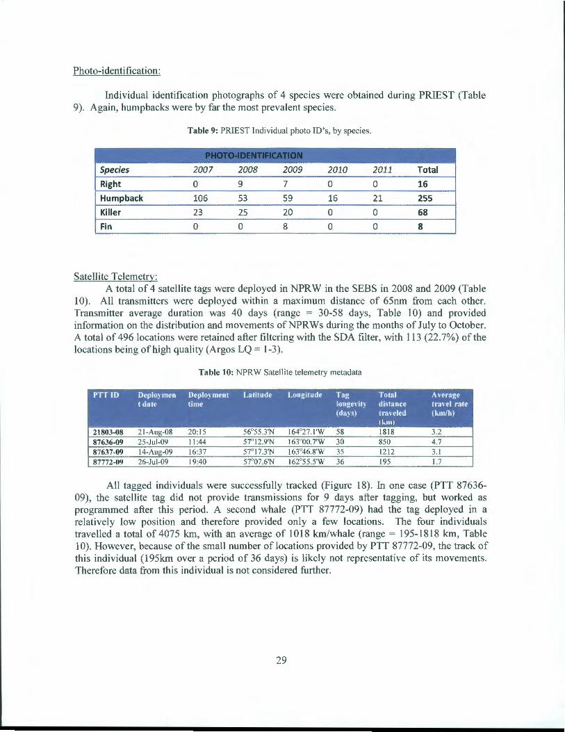
Satellite Telemetry: A total of 4 satellite tags were deployed in NPRW in the SEBS in 2008 and 2009 (Table

1 0). All transmitters were deployed within a maximum distance of 65nm from each other. Transmitter average duration was 40 days (range = 30-58 days, Table 1 0) and provided information on the distribution and movements ofNPRWs during the months of July to October. A total of 496 locations were retained after filtering with the SDA filter, with 113 (22.7%) of the locations being of high quality (Argos LQ = 1-3).

Table 10: NPRW Satellite telemetry metadata

PTT ID Oeplo~ men Oeplo~ ment Latitude Longitude Tag Total A\'erage t date time Ionge' it~ distance tra\CI rate

(da~ s) tra\eled (km/h) (km)

21803-08 21-Aug-08 20: 15 56°55.3'N 164°27.1'W 58 1818 3.2 87636-09 25-Jul-09 II :44 57°12.9'N 163°00.7'W 30 850 4.7 87637-09 14-Aug-09 16:37 57°17.3'N 163°46.8'W 35 1212 3.1 87772-09 26-Jul-09 19:40 57°07.6'N 162°55.5'W 36 195 1.7

All tagged individuals were successfully tracked (Figure 18). In one case (PTT 87636-09), the satellite tag did not provide transmissions for 9 days after tagging, but worked as programmed after this period. A second whale (PTT 87772-09) had the tag deployed in a relatively low position and therefore provided only a few locations. The four individuals travelled a total of4075 km, with an average of 1018 km/whale (range= 195-1818 km, Table I 0). However, because of the small number of locations provided by PTT 87772-09, the track of this individual (195km over a period of 36 days) is likely not representative of its movements. Therefore data from this individual is not considered further.

29

56N

54N

200m

170W

170W

Prlbilof Islands

~

165W

165W

160W

58N

56N

- 87636.09

87637.09 54 N

- 21803.08

160W

Figure 18: Tracks ofNPRWs tagged in the SEBS in 2008 and 2009. Stars represent tagging location (see also Table 7)

NPRW movements in the SEBS were restricted to a relatively small region between 56°-580N and 163°-167°W in the middle shelf to the west of Bristol Bay (Figure 18). This region corresponds to an area of nearly 26,400 km2

• Satellite locations show that none of the whales ventured into waters shallower than 50m and that they did not move in deeper waters (e.g. >80m) during the period they were tracked. The monthly average location of PTT 21803-08 (the only whale tagged in 2008) was further offshore than that of two whales tagged in 2009 (Figure 18). Average locations also suggest that NPRW s move offshore later in the season (Figure 19).

30

56 N

54' N

170W

Prlbilof Islands

100m

50m

165W

165W 160W

58N

56N

160'W

Figure 19: Individual satellite locations offour NPRWs in the SEBS in 2008 (crosses) and 2009 (asterisks). Circles and squares represent monthly averages in 2008 and 2009, respectively . Month color code: August = dark red,

September = red, October = Orange.

Attempts were made to approach whales within the range for tagging and biopsy sampling from rigid hull inflatable boats and, occasionally, from the larger survey vessel. NPRWs showed extreme avoidance behavior to all types of platforms used, not only for tag deployment, but also for photo-identification and biopsy sampling. Due to this behavior, satellite transmitters were deployed at ranges greater(> 8m) than the typical ranges preferred in this type of study (5-10m). Despite avoiding vessels, NPRWs showed little or no visible reaction to tag deployment per se and the animals were repeatedly seen displaying normal behavior in the hours and days following deployment or deployment attempts.

After tags were deployed, attempts were made to visually relocate tagged whales both immediately after deployment as well as in subsequent days during search for other individuals for tagging and other studies. The intention was to assess the conditions of the tag on the body of the whale as well as the physical condition of the animals before and after the tag stopped working. One individual (PTT 21803-08) was photographed 14 days after tagging (Figure 20). While the tag had shown a small degree of migration outside the body ofthe animal, no swelling, signs of infection or other evidence of physical injuries were observed. ln addition, a whale tagged in 2004 (Wade et al. , 2006) was re-sighted. Even though it was not possible to assess the site where the tag had been deployed, this individual showed no evidence of poor body condition or of being unhealthy.

31

Figure 20: PTT # 21803-08 shown at time of deployment (A), I day after deployment (B), and 14 days after deployment (C) .

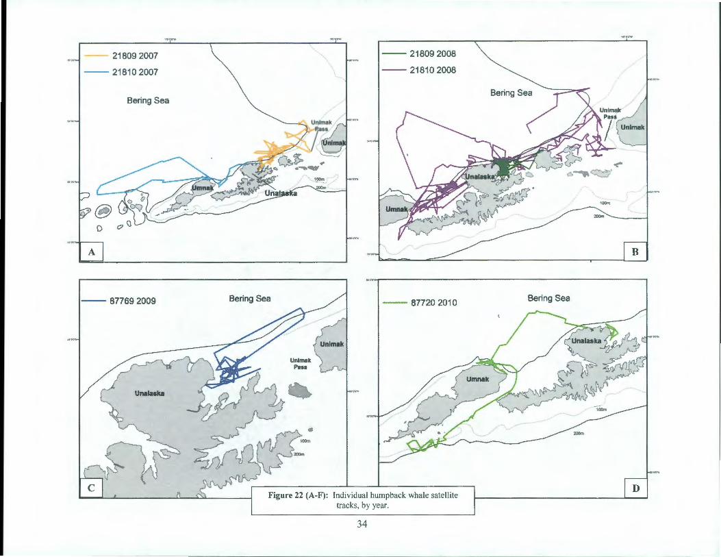
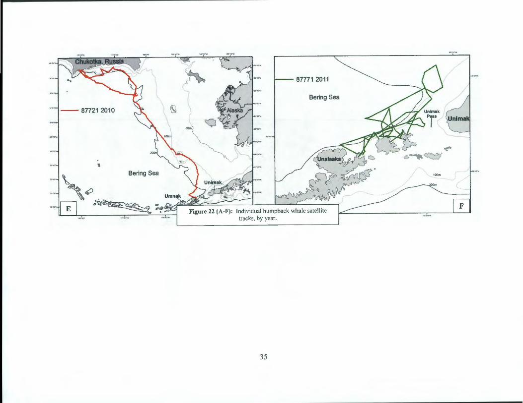
Additionally, there were ten satellite transmitters deployments in humpback whales during this study, yet only 8 tags transmitted long enough to be considered for further study (Table 11, Figure 21 ). The SPOT 5 tags were placed on the right or left dorsal surface of the whales' body using an Air Rocket Transmitting System (ARTS) (see Methods section). Most tags were in relatively good position and flush against the body of the whales. Individual whales were tracked for an average of 28 days (range= 7-67 days) (Table 11) and showed substantial variation in movements. Three individuals remained within 50km of their tagging locations for as many as 14 days (Figure 22b, c, f). Three whales explored presumed feeding areas within 60 km from shore, along the Bering Sea side of Unalaska Bay and Unimak Pass (Figure 22a, b, f). Two whales moved west; one made a trip to the Island of Four Mountains and returned to the northern side of Umnak Islands and a second whale moved through Umnak Pass and explored feeding areas on both the Bering and Pacific sides of Umnak Island (Figure 22a, d). One

32

individual left Unalaska Bay three days after tagging and moved ~ 1500km (in 12 days) along the outer Bering Sea shelf to the southern Chukotka, Russia. After 4 days, this individual moved east across the Bering Sea basin to Navarin Canyon (60°30'N, 179°20 ' W), where it remained until transmissions ceased (Figure 22e).

Table 11: Humpback whale satellite telemetry metadata.

Deployment Tag Longevity Total km

Avg. PTTID traveled

Date (d) (minimum)

km/day

8/1112007 28 892.2 31.9 21809.07 21810.07 8/ 11/2007 17 746.5 44.0

21809.08 8/26/2008 36 956.0 26.6

21810.08 8/26/2008 67 2636.9 39.4

87769.09 8/6/2009 7 219.3 31.3

87720.10 8/ 112010 15 550.1 36.7

87721.10 8/ 112010 26 3014.5 115.9

87771.11 9/ 10/20 II 29 1254.1 43.2

AVERAGE: 28 1283.7 46.1

Figure 21: Satellite transmitter (PTT 87721) attached deployed on a humpback whale in 2010.

33

21809 2007

- 21810 2007

Bering Sea

A

-- 87769 2009

-- 21809 2008

-- 21810 2008

Bering Sea -- 87720 2010

Figure 22 (A-F): Individual humpback whale satellite tracks, by year.

34

Bering Sea

,-~ ~

I

' \ 50m

Bering Sea

,_ 87771 2011

Bering Sea

Individual humpback whale satellite tracks, by year.

35

<?'"

Acoustics :

Right whales vs. Bowheads

Because a number of species like humpback and bowhead whales can all produce the same or very similar call types to right whales, with similar call characteristics, analysts relied heavily on context for distinguishing between species. For example, analysts would look for the presence of other known call types of humpback, bowhead, or right whales near the call in question. The general inter-call intervals and/or patterning of the questionable calls were also used .

We focused on the upsweep and gunshot call types for this analysis because of their common use in right whale acoustic studies (upsweeps) and overall abundance in the recordings (gunshots). Right whale gunshot calls are impulsive broad band signals, ranging from approximately 50 Hz to 4 kHz, with most energy below 2 kHz, and a duration of 0.25-1.25 s (Figure 23a). Right whale upsweep calls are frequency modulated calls between 80 Hz and 200 Hz, with a duration ranging from 0.5-1.5 s (Figure 23b ).

2.5

N 2 I .X:

;: 1.5 u c Q) :::J 0' Q)

u: 0.5

5 10 15 20 Time (s)

250

'N200 I

;: 150 u c ~ 100 0' ~ u..

5 10 15 20 25 30 35 40 Time (s)

Figure 23: Most common right whale sounds encountered during PRIEST. A) Gunshot calls B) Upsweeps. Color of spectrogram represents amplitude of sound (red= highest).

Both right and bowhead whales produce similar gunshot and upsweep calls (humpbacks produce upsweep calls, but these are easily distinguished through contextual clues). However, right whale gunshot calls follow a very similar seasonal trend to upsweeps, whereas bowhead gunshot and upsweep calls do not follow any trend. This correlation was primarily what we used to distinguish between species. However, in some cases, conclusions could not be made based on seasonal call correlations because of insufficient data, and the analysis was left as uncertain.

36

The overall findings in the results that follow are that gunshot and upsweep seasonal calling trends are more highly correlated the closer the recording is to the RWCH. Therefore, while we cannot rule out the possibility that right whales occur north of 60° N in the Bering Sea, historical whaling data and lack of any correlation in seasonal calling trends between gunshot and upsweep calls north of thi s 60° N line make it highly likely that the upsweep and gunshot calls detected on recordings are produced by bowhead whales.

Sonobuoys

Sonobuoys were deployed in all four years of the PRIEST survey, and also during the transit leg through the Bering Sea for the 2011 CHAOZ survey. Figure 24 shows a composite map of the locations of sonobuoys on which right whale sounds were detected (no right whales were detected in 2007). Figures 25-29 show the location of all sonobuoy deployments and species detected during the 2008-20 II field seasons, respectively.

'• '

Right whale detections

\~

• 2011

2010

• 2009

• 2008

O escH - NAB lease area

•

• ,-- -

106"0'W

N

A 35 ro 1.00 Km

1as·ow 180"0W

Figure 24: Location of sonobuoys with right whale acoustic detections 2007-20 II.

37

55"0'N

The first field season, 2007, was plagued by sonobuoys that malfunctioned in mass (59% success rate). Even when the sonobuoys functioned, results were disappointing in regards to the lack of sounds present on the recordings. Of the 79 successfully deployed buoys, 6 (7.5%) recorded humpback sounds, 8 (10.1 %) had fin calls, and 8 (10.1 %) had other or unknown marine mammal calls (Figure 25). No right whale calls were detected during this survey.

170VW

• Acoustic Detections

X Finwhate

• Humpback whale

? Other/unknown

• No detections

c::::J sscH - NAB tease area

170~

?

• •

X

" •

t65"0W

165'0W 110"0W

35 70 140 Km

1eG'OW

Figure 25: Location of and species detected on all sonobuoys deployed during the 2007 PRI EST survey.

'17N

A total of 302 sonobuoys were deployed in 2008 (Figure 26), with much greater success (78.5%) than in 2007, thanks to the efforts of Jeff Leonhard (Naval Surface Warfare Center, Crane Division) and Theresa Yost (Naval Operational Logistics Support Center) in providing us with more recently expired sonobuoys (the sonobuoys used in 2007 were 30 years old). Of the 237 successfully deployed buoys, 74 (31 %) had right whale gunshot calls and 21 (9%) had some variation of right whale upsweeps. In addition, humpback, fin , and orca whale sounds were detected on II (5%), 58 (25%), and 10 (4%) ofthe sonobuoys respectively.

38

<:;::1' . . . X

Acoustic Detections

e Rtght whale

Kil ler whale

II Humpback whale

X F1nwhale

• No detections

c:::J BSCH

- NAB lease area

110'0W 16S'"OW

X X ;.:

16.5"0'W IIO'O'W

Figure 26: Location of and species detected on all sonobuoys deployed during the 2008 PRI EST survey.

' O'N

In 2009, 262 sonobuoys were deployed successfully (Figure 27). Of these, 157 (60%) recorded right whale gunshot calls, 53 (20%) recorded right whale upsweep calls, 30 (11 %) recorded humpback sounds, 167 (64%) had fin calls, 14 (5%) had killer whale calls, and 20 (7%) had other marine mammal calls. Improvements in the sonobuoy tracking software in 2009 allowed for much more accurate localizations of the vocalizing right whales, substantially reducing the amount of vessel time spent searching for the whales compared with the previous seasons. This increased the amount of time the research team could spend with photo­identification, biopsy, and satellite tagging of the whales.

39

... Acoustic Detections

• R<ght whale

K1ller whole

• Humpback whale

X F1n whale

o No detec:IJons

D ascH - NAB lease area

17tr'C1'W

IOOVW

X

5S"O'N

36 10 ••o Km

165"0W IOO'O'W

Figure 27: Location of and species detected on all sonobuoys deployed during the 2009 PRIEST survey.

Gunshots calls were the most common right whale vocalization detected in 2010 (Figure 28), present on 33% of all buoys successfully deployed in the Bering Sea. Right whale upsweep calls were detected on 17% of the buoys. The most common species detected was the fin whale, detected on 55% of the buoys. Other species detected include humpback whales (detected on 17% of the buoys), killer whales (5% of the buoys), and one minke whale detection . Overall, fewer buoys were deployed and fewer species detected in 2010 than in the previous two years. This was due to the inclement weather experienced throughout the survey. Many of the buoys were deployed during transit to and from the area, where species are historically less likely to be present. Fewer days were spent in the right whale Critical Habitat than in the previous two years, which accounts for lower number of acoustic detections. We were never able to remain in the Critical Habitat for more than two days before having to find a lee from the weather. During the 20 l 0 Bureau of Ocean Energy Management (BOEM) funded Chukchi Acoustics, Oceanography, and Zooplankton (CHAOZ) survey (Aug 24 - Sept 20), two days were spent in the Right Whale Critical Habitat during the vessel's return transit to Dutch Harbor (Sept 18-19). Once the vessel was within the Critical Habitat, 24 hour passive acoustic monitoring was conducted (increased from every 3 hours) to maximize the likelihood of detection . A right whale was detected on the morning of September 181

h. Sonobuoy detections during the right whale portion ofthe CHAOZ cruise are included in the figures mentioned above for 2010.

40

175'W 170"W IOO'W

• • OO'N •

X •

X ~ · X~

X

X ... X

....

X

~

.... Acoustic Detections

• Right whale

Killer whale

• Humpback whale

X Fin whale .. Minke whale

S4' N ? Unknown

CJ ascH

-- NAB lease area

t75"W , .. 'W IOO'W

Figure 28: Location of and species detected on all sonobuoys deployed during the 2010 PRI EST & CHAOZ surveys.

During the Bering Sea legs of the 2011 CHAOZ survey, the acoustics team deployed a total of 142 sonobuoys with an overall success rate of 84% (Figure 29). Right whale gunshot calls were present on 15% of the buoys, and right whale upsweep calls were present on 4% of the buoys. Fin whales were the most common species detected, present on 46% of the buoys. Humpbacks were detected on 39% of the buoys, killer whales were present on 18% of the buoys, and sperm whales were detected on 2% of the buoys. The lower number of acoustic detections for 2011 versus 2008 & 2009 was due to the fact that most of the buoys were deployed during transit to and from the area in 2011. During the Dutch Harbor - Nome transit leg of the 2011 CHAOZ survey (Aug 12-17, 2011), right whale gunshot calls were detected on August 13th at around noon. The DiF AR bearings to the vocalizations resulted in a position directly in the path of the vessel, and two hours later, four right whales were seen by the visual observers as described above. This was the only day right whale calls were detected during that leg. On the return transit to Dutch Harbor from Nome (Sep 3-11 , 2011 ), right whale calls were detected in the same general area where they were seen on the first transit leg, and although we tried to wait out the bad weather for an extra day, the forecast was predicting even higher sea states (which occurred), and so we left the area before getting a chance to work with those animals. We detected right whales for a total of two days on this return transit leg.

41

180 175'W 170'W 165'W 180'W 155'W

? 62N

• . . . • • N

• • 1

60N

•

• ·x 58N

58"N

Acoustic detections

• Right whale

se·N Killer whale

• Humpback whale

X Fin whale 58"N

• Sperm whale

? Unknown

• No detections 54"N

c:J BSCH -- NAB lease area 54"N

Figure 29: Location of and species detected on all sonobuoys deployed during the 20 I I CHAOZ survey.

Aerial Acoustics

There were a total of 58 sonobuoys used in deployed from the aircraft by the aerial survey team during this project. Two 53E units were activated on the ground to help with troubleshooting and testing of the equipment. Of the 56 deployed while on survey, 38 77C units were used with 3 failures while 18 53E units were deployed with 4 failures. Preliminary analysis and in-flight observations showed that right whale gunshots (51%) and upsweeps (35%) were detected, as well as fin whale calls on a majority of deployments (59%), and the occasional (20%) humpback call (Figure 30).

Sonobuoy tracking software allowed for very accurate localizations of the vocalizing right whales, and so the amount of time the aircraft spent searching for the whales during 2009 was much less than that from 2008. This increased the amount of time the research teams could spend with photo-identification, biopsy, and satellite tagging of the whales. (See Appendix A, pg. 102 for further details).

42

165'W

ss•N

165'W

RW Upsweep

RW Gunshot Humpback Fin

160'W

0 D ... X

No Detections 0 Survey Effort RW Visual Sightings *

160'W

Figure 30 - Aerial sonobuoy detection results for the 2009 PRIEST survey.

Long-term moored acoustic recorders

Analysis was completed for a total of 22 recorders: I 0 A URALs, 3 Haruphones, and 9 EARs. Right whale gunshot (Figure 23a) and upsweep (Figure 23b) calls were processed separately so that analysis for each could focus on its main frequency bandwidth.

In all figures that follow in this section, right whale gunshot calls are shown in blue, while upsweep calls are shown in red . For consistency, all figures also have their X-axes scaled to run from May of one year to November of the following year. Although each recorder type was processed on a different time interval (i.e., AURALs and Haruphones were processed in 3 hour time increments, while EARs were processed entirely) the results were compiled on a 3 hour time interval for all recorders. Therefore, each data point represents the percentage of 3 hour time intervals for that week (i.e. 56 total) that contain at least one right whale call of that type.

Two Haruphone recorders, funded by a North Pacific Research Board project (Drs. Kate Stafford (APL!UW) and David K. Mellinger (PMEL/Oregon State University)), were deployed

43

on PMEL Bering Sea moorings M2 and M4 in 2007. Although these recorders were not part of the PRIEST project nor were they funded by NOAA, the data are of relevance to the study years of this project and are included in our analysis. The M4 mooring data (Figure 3lc) show two common trends seen throughout the study. First, the seasonal occurrence of upsweep calls follows the same pattern as that for the gunshot calls. Second, gunshot calls occur during a much higher percentage of time intervals overall than the upsweeps. For 2007 the peak in both gunshot and upsweep calls occurred mid-October 2007 through January 2008. Because the seasonal trends of both these call types are similar, it seems likely that these are in fact attributable to right whales. More than half the data from the M2 mooring (Figure 31 d) were lost when one of the hard drives extracted from the Haruphone at the PMEL facility in Newport, OR was dropped. Unfortunately, the lost data would have been recorded during the prime right whale calling time on that mooring (May-Dec). The number of calls of either type in the data available for this mooring are not numerous enough to show conclusive results, other than neither call type was detected at substantial levels from Jan-May, 2008. Figure 32 shows these seasonal call plots superimposed onto a map of their mooring locations in the Bering Sea. Spatial trends cannot be determined from this figure since the first half of the M2 data is missing. From Jan-May 2008, both the M4 and M2 moorings show a similar lack of calling.

A

100

!10 c

3 70

I eo

i 50 .1:

~ .. L : 30

20

10

0 . ~7 .hA-07 5el>-07 No-..07 Jon.08 M.-.oe Moy.oe Jul.o8 So!>(l8 NoY.o8 -y-

B

100

!10 D

10

Figure 31: Right whale seasonal call distribution of gunshot (blue) and upsweep (red) calls on PMEL moorings 2007-2008: A) M8 B) M5 C) M4 D) M2 (first data disk in M2 was dropped and data were unrecoverable). Note:

results are for all gunshot and upsweep calls, not necessarily specific to right whales. See text for explanation.

44

180'0' 115"0W

•

\ •

55"0'N

175VW 170"0W

170"0W

! • t.

I·

155•ow

M4

~~ L ..:,...._._....,_,"'=-=-----

165"0W

155"0W

'0>1

125 250 Kilometers

IOO"OW

Figure 32: Results from 2007-2008 Haruphone recorders superimposed on map of mooring locations. See Figure 29 for larger versions of the Haruphone data plots. Blue pentagon = RWCH, red polygon = NAB lease area, yellow pentagons = PMEL moorings. On inset seasonal calling figures: blue = gunshot calls, red = upsweeps. Note: results

are for all gunshot and upsweep calls, not necessarily specific to right whales. See text for explanation.

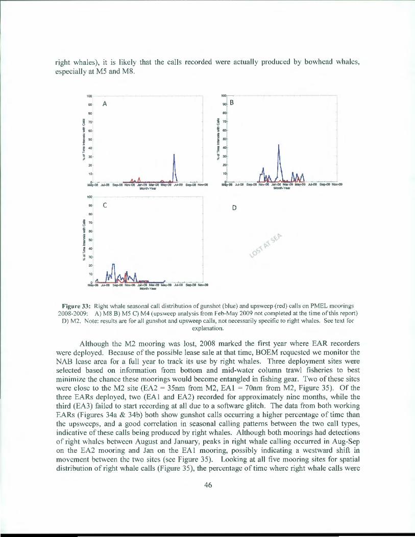
Two Haruphones (at M2 and M4), two AURALs (at M5 and M8), and three EARs were deployed in 2008. The bad luck continued with the M2 recorder, with the entire 2008 mooring lost at sea. Recordings from the M4 mooring (Figure 33c) show a different pattern in calling as compared to the M4 mooring from 2007 (Figure 3lc). First, the gunshot call pattern is more spread out in 2008 than in 2007, occurring from Jul-Dec. Second, the peak occurs much earlier in July 2008 than in November for the 2007data. Lastly, this peak is half the size of the peak seen in 2008. The upsweep calling in 2008 does not track well with the gunshot calling, although there is some correspondence in the Sep-Oct time period. Very little correlation is seen between gunshot and upsweep calls with the M5 mooring (Figure 33b) and no correlation is see with M8 (Figure 33a). For all recorders, a much higher percentage of time intervals were found to contain gunshot rather than upsweep calls. The M5 recorder had the highest peak in percentage of time intervals containing gunshot calls (~45% in mid-January 2009, Figure 33b). However, since very little to no correlation is found with the gunshot/upsweep calling trends (as is common with

45

right whales), it is likely that the calls recorded were actually produced by bowhead whales, especially at M5 and M8.

100

90 A llO

s 70

t 80

I 50 :E ! 40 ...

:: ~ 10

0 • ~ ..-...oe Sel>-08 No¥.()8 - -.og May-oil Jl.f.09 Sej>()9 --y-100

90 c 80

s 70

t 80

1 50 .li ~ 40

: 30

100

90 B llO

D

Figure 33: Right whale seasonal call distribution of gunshot (blue) and upsweep (red) calls on PMEL moorings 2008-2009: A) M8 B) MS C) M4 (upsweep analysis from Feb-May 2009 not completed at the time of this report)

D) M2. Note: results are for all gunshot and upsweep calls, not necessarily specific to right whales. See text for explanation.

Although the M2 mooring was lost, 2008 marked the first year where EAR recorders were deployed. Because of the possible lease sale at that time, BOEM requested we monitor the NAB lease area for a full year to track its use by right whales. Three deployment sites were selected based on information from bottom and mid-water column trawl fisheries to best minimize the chance these moorings would become entangled in fishing gear. Two of these sites were close to the M2 site (EA2 = 35nm from M2, EA 1 = 70nm from M2, Figure 35). Of the three EARs deployed, two (EAl and EA2) recorded for approximately nine months, while the third (EA3) failed to start recording at all due to a software glitch. The data from both working EARs (Figures 34a & 34b) both show gunshot calls occurring a higher percentage of time than the upsweeps, and a good correlation in seasonal calling patterns between the two call types, indicative of these calls being produced by right whales. Although both moorings had detections of right whales between August and January, peaks in right whale calling occurred in Aug-Sep on the EA2 mooring and Jan on the EAl mooring, possibly indicating a westward shift in movement between the two sites (see Figure 35). Looking at all five mooring sites for spatial distribution of right whale calls (Figure 35), the percentage of time where right whale calls were

46

detected decreased going north, with really low numbers at the M4 site. Again, the lack of correlation between call types for the M5 and M8 sites indicates that this calling is actually from bowhead and not right whales at these sites.

100 r

90

80

a 701

J 60 1

i :t ~

201

A

i (,)

J .!1

~ .5

~ ll ~

c

100

90 B

80 •

70

60

50

40

30

20

10

0 ...... - -'--May-08 Jul-0!! Sep-08 Nov-08 Jar>-09 Mar-o9 May-o9 Jul-o9 SeiH)9 ~

MCW'Wh-Yew

Figure 34: Right whale seasonal call distribution of gunshot (blue) and upsweep (red) calls on EAR moorings 2008-2009: A) EAOI B) EA02 C) EA03 (Malfunctioned). Note: results are for all gunshot and upsweep calls, not

necessarily specific to right whales. See text for explanation.

47

• M8 ! • I •

00'0" I· ! .

~--~---

17S"''W 170'0W

" MS ! • ,_ I·

165'DW IOO'OW

o-----1 :• ,. &L

17$'0W

! • t.

I· I • : . ~~----

. .. l= u I • l.

..:....----·-----

.

.:..----------

: l EA2 I· , .

.....-'----1 :•

o4----·::::::·---- 5 125

165'0W

15S'OW

250 Kilometers

..... w

Figure 35: Results from 2008-2009 EAR and AURAL!Haruphone recorders superimposed on map of mooring locations. See Figures 33 and 34 for larger versions of the AURAL!Haruphone and EAR data plots, respectively. Blue pentagon = RWCH, red polygon = NAB lease area, yellow pentagons = PMEL moorings, blue diamonds = EAR moorings. On inset seasonal calling figures: blue = gunshot calls, red = upsweeps. Note: results are for all

gunshot and upsweep calls, not necessarily specific to right whales. See text for explanation.

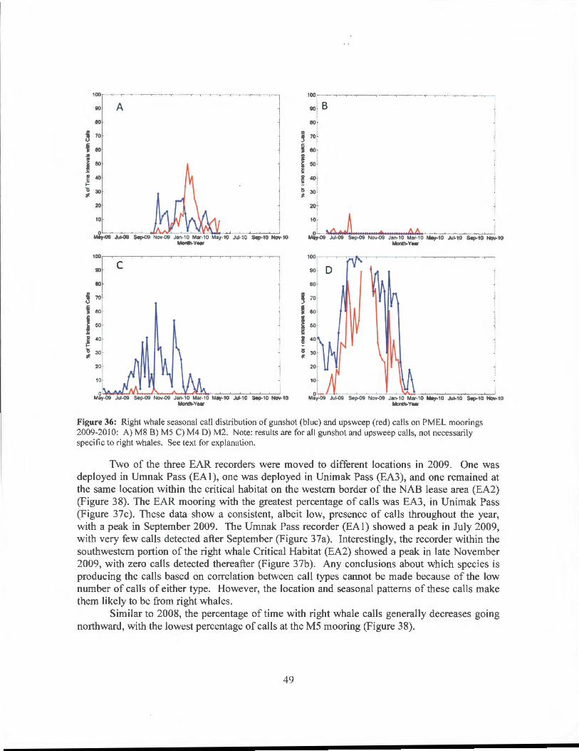
Four AURAL recorders were deployed at sites M2, M4, M5 and M8 in 2009. The mooring with the greatest percentage of calls was M2, with a peak from July 2009 - January 20 I 0 (Figure 36d). In addition to the high percentage of calls present on M2, there is a strong correlation between upsweeps and gunshot calling patterns, suggesting that these calls are attributable to right whales. There were considerably fewer upsweeps than gunshot calls at M4, and as a result there is very little or no correlation between gunshot and upsweep calling patterns (Figure 36c). While there are a greater percentage of calls at M8 than at M5, neither show a correlation between gunshot calls and upsweeps, suggesting that these calls may have been produced by bowhead whales, not right whales.

48

90 A 80

~ 70

l 60

j 50

~ 40

; 30

20

10

0 ..L. ,1. ...... A. J

~ l ! E ! 15 ,_

100 ~, -"T --,

:[B 70 t

:I 40 >

30 ,

lOt A

M<!y-()9 Jul-09 Sep-09 Nov-()9 Jar>-1 0 Mar-10 May-10 Ju~1 0 ~10 Nov-10 -y- o J\ •J\ + AA "' ... May-()9 Jul-09 Sep-09 Nov-o9 Jar>- 10 Mar-10 May-10 Jul-10 ~10 Nov-10

Monii>-Y-

~ l I .E

! >--~ .,.

100

1 90

c 80

70 j 80

50

40

30

20

0 ...&... ..........

May-()9 Jul-()9 Sep-09 Nov-()9 Jar>-10 Mar-1 0 May-10 Ju~10 ~10 Nov-10 -Year

901

so[ D

i 70 _,

l 60

II § 50

= ! 15 ,_

Figure 36: Right whale seasonal call distribution of gunshot (blue) and upsweep (red) calls on PMEL moorings 2009-20 I 0: A) M8 B) M5 C) M4 D) M2. Note: results are for all gunshot and upsweep calls, not necessarily specific to right whales. See text for explanati on.

Two of the three EAR recorders were moved to different locations in 2009. One was deployed in Umnak Pass (EAl), one was deployed in Unimak Pass (EA3), and one remained at the same location within the critical habitat on the western border of the NAB lease area (EA2) (Figure 38). The EAR mooring with the greatest percentage of calls was EA3, in Unimak Pass (Figure 37c). These data show a consistent, albeit low, presence of calls throughout the year, with a peak in September 2009. The Umnak Pass recorder (EAl) showed a peak in July 2009, with very few calls detected after September (Figure 37a). Interestingly, the recorder within the southwestern portion of the right whale Critical Habitat (EA2) showed a peak in late November 2009, with zero call s detected thereafter (Figure 37b). Any conclusions about which species is producing the calls based on correlation between call types cannot be made because of the low number of calls of either type. However, the location and seasonal patterns of these calls make them likely to be from right whales.

Similar to 2008, the percentage of time with right whale calls generally decreases going northward, with the lowest percentage of calls at the M5 mooring (Figure 38).

49

100

90 A

80

i 70 () .r:. J 60

I 50

~ 40 .... l> 30 .,.

20

10

O 'l,..,A A + , , May-()9 Jul-09 Sep-09 Nov-09 Jan-10 M¥-10 May-10 Ju~10 Sep-10 Nov-10

Month-Year

100

90 • c

s 70 1

J so l

1 50 t

~ 40

~ 30

20>

100 -r '"T ...,.. T'

90

60

~ 70

J 60

j 50

! 40

~ 30

B

Figure 37: Right whale seasonal call distribution of gunshot'(blue) and upsweep (red) calls on EAR moorings 2009-20 I 0: A) EAO I Umnak Pass B) EA02 RWCH C) EA03 Unimak Pass. Note: results are for all gunshot and

upsweep calls, not necessarily specific to right whales. See text for explanation.

Four AURAL recorders were redeployed at sites M2, M4, M5 and M8 in 2010. Although the recording from first deployment of the M2 mooring (May-Sep 201 0) failed after 23 days, data from the second deployment (Sep 201 O-May20 11) again shows this mooring site has the highest percentage of time intervals with right whale calls, with a near constant presence of gunshot calling in November (Figure 39d). The M2 data also show a strong correlation in seasonal trends of the upsweeps and gunshot calls, indicating that right whales are most likely making these calls. The M4 recordings have a much lower level of both call types (Figure 39c ), with a peak in gunshot calls in October under 50%. The correlation between the two call types is weaker than at M2, indicating uncertainty in the species making the calls, with a peak in upsweep calls occurring later in December. Unfortunately the M5 recordings were contaminated by mooring noise (chain rattling, etc), which made it impossible to see or hear any right whale calls, except for a few upsweeps at the very beginning of the deployment (Figure 39b ). In contrast to the M2 and M4 recordings which had more time intervals with gunshot calls than upsweeps, M8 (Figure 39a) was the opposite, with a peak in upsweeps over twice the height of

50

the gunshots. Because of this, and because the two call types show no correlation, it is highly likely that these calls are from bowheads, and not from right whales.

17S"OW

• M8 ! •

- ~~ A .L..--- ........ ___ .. ___ _

......

175'0W

• MS ! • I •

I · I" :·

. ! • I •

I · ,. :.

. ! • I •

I · I • :.

EA3

• ,)y,),<o . .. ._. -4-- - -· :. .. - . -= ---·

EAl

• 1-.......... ""'----~·-· .. ·-·-·

110"0W

I· I • ..

11S'OW

~A· : ----;;::.-::. -·-·-·-·

. ! • I •

I · I • .__...., :. .

110'0W

EA2

:. - e'lj -;;::.-::;·-· -· -·-· 2.5 125

165"0W

ISS "'W

250 Kilometers

Figure 38: Results from 2009-2010 EAR and AURAL recorders superimposed on map of mooring locations. See Figures 36 and 37 for larger versions of the AURAL and EAR data plots, respectively. Blue pentagon = RWCH, red

polygon = NAB lease area, yellow pentagons = PMEL moorings, blue diamonds = EAR moorings. On inset seasonal calling figures: blue = gunshot calls, red = upsweeps. Note: results are for all gunshot and upsweep calls,

not necessarily specific to right whales. See text for explanation.

To get a better sense of the extent to which right whales use the Bering Sea shelf, and to monitor for other species of interest (i.e., humpback and fin whales), three EAR recorders were spread along the 50m isobath, while the fourth remained in Unimak Pass. Not surprisingly, the mooring site with the highest percentage of right whale calling was EA3 in the RWCH (closest to the M2 mooring), with a peak in gunshot calls of over 80% in November. The trend in upsweep calls tracked well with the gunshots, at about half the level (Figure 39c), indicating that these calls are produced by right whales. 20 I 0 was a big disappointment for EAR recorders, however, with one recorder (Mooring EAOl -Figure 39a) failing after about a month with no calls of either type detected, and the Unimak Pass mooring (EA04 - Figure 39d) having very faint recording due to a faulty hydrophone. Very faint humpback whales were detected at on some days at the Unimak Pass mooring, but no right whale calls were detected. Given the

51

interesting results from this mooring in 2009, it was extremely frustrating to have this failure in 2010.

The spatial trends in calling patterns seen in 2010 (Figure 41) again show a northward decrease in both calling types, with a stronger correlation between the two calling types to the south, indicating that the northern detections are more likely not right whale than those to the south. In addition by following the timing of calling peaks on these recorders with more certain right whale detections, there appears to be a possible southern movement of whales between the EA03 and M2 mooring sites.

100 T . T r T T T T T T T

90 A 80

'i 70 .., t 80

I :1 .... '!! 30 "#

. Sep-1 1 Nov-11

100

90 > c 80

~ 7of j 60 >

j 50r

! <10 .... ~ 30"

20 •

10[

0 ..I. ..... . ...... .....

May-10 Ju~10 Sep-10 Nov-10 .1¥>-1 1 Mar·11 May-11 Jul·11 Sep-1 1 Nov-11 ~Year

100 T T T '

90 ' B J ..

jj 70 .., t 80

t 50

·:(\~ 0(.

0 s ~ .... '!! "#

~ j .!! . ! ~ .... '!! ;1.

·~~ <10

30 0 20

10

0 ... . --1.- ....

May-1 0 Ju~ 10 Sep-10 Nov-10 ~r>- 11 Mar-11 May-11 Ju~11 Sep-11 Nov-11 ~Year

·:ro ~ ~ .,. ~ r ~

70

60

50

<10

30

20

10

0 ,........;.... ..;.. ~

May-10 Ju~ 10 Sep-10 Nov-10 ~r>-11 Mor· 11 May-11 Ju~11 Sep-11 Nov-11 Mond\-Yet!Jif

Figure 39: Right whale seasonal call distribution of gunshot (blue) and upsweep (red) calls on PMEL moorings 2010-2011: A) M8 B) M5 C) M4 D) M2. Note: results are for all gunshot and upsweep calls, not necessarily

specific to right whales. See text for explanation.

The 2011 recorders are off to a good start, with the first deployment of the M2 mooring (May -Sep 2011) recording for the entire deployment (Figure 42d). The number of time intervals with right whales detections began to climb in June and reach 90% levels from August until the mooring was retrieved in September. Interestingly, not only did the trend in upsweep calling follow that of gunshot calls closely, the levels of both were well-matched, indicating these calls are produced by right whales. As this mooring is in the R WCH (Figure 43), the results for this mooring are expected.

52

100

90 A

80

" 'i 70 (.)

~~<y "' ·J 60

" ~ l 50 ~~~ :E .! 40 <:;)~ .... 0~ l> 30 <y(; # ~

20

10

0 ~ May-10 Ju~10 ~W~IO,Jan-11 Mar-11 May-11

Month-Year

100

90 (

~ (.)

"' 1

1 ;5

I .... l> ;f.

Ju~11 Sep-11 Nov-11

s "' 'J " l :5: .~ .... l> ;f.

100

90 B

80

70

60

50

40

30

20

10

0 ~ 1y. A A " Mliy-10 Ju~10 ~10 Nov-10 Jan-11 Mar-11 May-11 Ju~11 ~11 Nov-11

Month-Year

100

90 D

80

70

60

50

40

30

20

10

Mgy-10 Ju~10 ~10 NOY-10 Jan-11 Mar-11 May-11 Ju~11 ~~~ Nov-11 Monll>-Year

Figure 40: Right whale seasonal call distribution of gunshot (blue) and upsweep (red) calls on EAR moorings 20 I 0-20 II : A) EAO I (recorder failed) B) EA02 C) EA03 D) EA04 (hydrophone malfunctioned). Note: results are

for all gunshot and upsweep calls, not necessarily specific to right whales. See text for explanation.

53

.... ,.

55-cl'N

• M8 ! • t.

I· ,. )•

175"QW

100"0' 175'0W

,J,. .............. - .. ";;.!.o:."-'' .... ' ..... -··

• M4 ! • t.

I· I • ~Ah I )• V/L

..... -· -· _,. ':!!.':" _ ...... , ...... _,.

170'0W

170'0'W t&S'OW 160'0W 155'0'W

• EA2

+ +-

<I· \ ,. :•

*· .... ·-·-.. ":!.:..~·- ........... _ ..

62.5 125 250 Kilometers

165'0W teo"OW 155'0W

Figure 41: Results from 20 I 0-20 II EAR and AURAL recorders superimposed on map of mooring locations. See Figures 39 and 40 for larger versions of the AURAL and EAR data plots, respectively. Blue pentagon = RWCH, red

polygon = NAB lease area, yellow pentagons = PMEL moorings, blue diamonds = EAR moorings. On inset seasonal calling figures: blue = gunshot calls, red = upsweeps. Note: results are for all gunshot and upsweep calls,

not necessarily specific to right whales. See text for explanation.

54

A

c

B

1:1 D

80

~ 70

j 80

I 50 .li ! 40 .... '15 30 .,.

20

10•

01 May-11 Jul-11 Sep-11 Nov-11 Jan.12 Mor-12 May-12 Jul-12 Sep-12 Nov-12 -..,.y..,

Figure 42: Right whale seasonal call distribution of gunshot (blue) and upsweep (red) calls on PMEL moorings 20 II: A) M8 B) M5 C) M4 D) M2. Except for the first deployment of M2 in 20 II , all recorders are still at sea, awaiting retrieval in 2012. Note: results are for all gunshot and upsweep calls, not necessarily specific to right

whales. See text for explanation.

55

,....,. li!'OW 1eG'OW

• •

\ •

• ~=, •• I· ,. : .

..:,. •• » _ .. _ .. ··:.:~ • .'::.· _ ., _ .. _, - ·

M2

0 82.5 125 250 Ki lometers

17$'0'W IJO"V<N ..... w

Figure 43: Results from 20 II AURAL recorders superimposed on map of mooring locations. See Figure 42 for larger versions of the AURAL data plot. Except for the first deployment of M2 in 20 II, all recorders are still at sea,

awaiting retrieval in 2012. Blue pentagon = RWCH, red polygon = NAB lease area, yellow pentagons = PMEL moorings, blue diamonds = EAR moorings. On inset seasonal calling figure: blue = gunshot calls, red = upsweeps.

Note: results are for all gunshot and upsweep calls, not necessarily specific to right whales. See text for explanation.

Near-real-time auto-detection buoy

See Appendix B (pg 119) for full Cornell report which contains the results from this deployment.

56

DISCUSSION

The present study is the first to provide a description of the fine-scale distribution and movements of NPRWs in their feeding grounds in the SEBS. Wade eta/ (2006) deployed a satellite tag on one NPRW in the SEBS in the summer of 2004. This whale was monitored for 40 days and stayed primarily on the SEBS shelf and outer shelf. However, the duty cycle of the tag was set to transmit locations only on every 3rd day, in order to preserve battery life (Wade et a/. 2006) Therefore, a fine-scale description of that animals movements was not possible. The small number of individuals tagged precludes more sophisticated statistical analysis.

One interesting finding of the present study is that right whales do not seem to venture into the inner shelf in the SEBS (waters shallower than 50m). It is still unclear why there is a marked preference for the middle shelf domain, but preliminary results indicate that this may be related to the presence of oceanographic features of importance to the right whale ' s prey. Baumgartner et a/. (2009) showed that right whales were associated with a subsurface front in the SEBS during oceanographic studies conducted in the summer of 2008. Waters deeper than 50m were colder, higher in salinity and presented higher phytoplankton and zooplankton biomasses.

Human Impact and Management Implications

Current threats to NPR Ws in the SEBS are poorly known, but given the small population size (~30 individuals, Wade eta/., 2010) any possible human activity (e.g. shipping, fishing, oil exploration) likely represents some risk to recovery. It has been suspected that the behavior of right whales may make them more vulnerable to ship strikes than any other large whale species (IWC, 2001 ). In fact, collision with vessels is, together with entanglement in fishing gear, the main source of mortality among North Atlantic right whales in the eastern coast of the US (IWC, 200 l ). The results presented here indicate that the summer range of the species partially overlaps with shipping lanes and some heavily fished areas (e.g. Nuka Research and Planning Group, 2005) and therefore increasing human activities in the SEBS will likely expose NPRW to greater threats. Therefore, further development of such activities (e.g. oil and gas exploration and increased shipping in the Bering Sea and Bering Strait) needs to be carefully planned.

Findings of this study have important implications for management. For example, the NMFS designated areas within the Gulf of Alaska and Bering Sea as Critical Habitat under the US Endangered Species Act (NMFS, 2006). The proposed boundaries in the SEBS (Figure 1) were developed based upon modem (post-1980s) summer records and are believed to reasonably represent the area in which NPRW's prey concentrations are most likely to occur. However, the designation was made on sparse information collected during studies that were conducted from the late fall to early spring. NMFS (2006) noted that further review of Critical Habitat should be conducted in the future , but this required additional data on distribution, habitat use, and movements.

The results of this study show that whales monitored via satellite telemetry remained inside the NPRW Critical Habitat in the Bering Sea (Figures 18-19). This has provided additional evidence that the Critical Habitat encompasses an important range of the population during their feeding season. Analysis of sonobuoy recordings from the 2008-2011 summer field surveys revealed a high site fidelity in the northeastern portion of the Critical Habitat as well (Figures 29-30). Furthermore, long-term recorders located throughout the BS shelf not only

57

confirm this northeastern site fidelity within the Critical Habitat, but have expanded seasonal presence to encompass the months of July through January.

Results presented here are also relevant to further decisions with regard to future exploration of oil and gas in the SEBS. In fact, NPR W satellite telemetry was conducted in association with a large-scale study of the distribution, abundance and habitat use of the species in the SEBS. This large-scale study was prompted by the need for better data to assess the potential impact of oil and gas development in the NAB lease sales area. The whales tracked during the present study largely remained to the north of this area, with only one individual (PTT 87636.09) making an incursion within the NAB for a period of 2 days. Movements of this individual therefore indicate that the NAB area is occasionally used by right whales during their feeding season. Long-term recorders deployed in the NAB lease area in 2008 and 2009 show that right whales are present from at least September through January in the western portion of the lease area (Figures 34 and 37). Usage of this area may vary according to environmental variables suggesting the need for a longer-term evaluation.

Finally, the continued loss of sea ice in the Arctic brings with it the certainty that shipping through the Northwest Passage and Northern Sea Route will increase dramatically in future years. The potential for impact on right whales in the Bering Sea through increased noise and collision risk cannot be overestimated.

Humpback Whale Telemetry

This study was also the first to provide a description of the fine-scale distribution and movements of North Pacific humpback whales in their feeding grounds in the eastern Aleutian Islands. The results largely support the findings of historical and current studies showing that humpbacks congregate in shallow, highly productive coastal areas in the North Pacific and Bering Sea. Satellite telemetry from this study makes it evident that individual whales are making independent decisions about fine-scale movement and that these decisions can lead to long-distance travel within a feeding season. The significant individual variation in movement shown here is difficult to predict or describe and could impact conservation and management strategies.

While specific information about threats to NPHWs is not available for all areas of their range, anthropogenic injury or mortality are comparatively well documented in US waters. Entanglement, a major source of mortality in the North Atlantic population (Johnson eta/. 2005; Northridge, 1991; Glass eta/., 2009), has been observed in Alaskan waters (Angliss, 2008), and a review of SPLASH photographs found that over 20% of NPHW s had rope entanglement scars (Calambokidis eta/., 2008) range-wide; the number jumps to 78% entanglement scars in SEAK (Nielson, 2009). Ship strikes are increasing in Alaskan waters (Gabriele et al., 2007) and involve a wide range of vessels. Impacts on humpbacks in the Eastern Aleutian Ialsnds (EAls) and Bering Sea will likely increase with the influx of human activity from newly ope ned oil and gas lease areas in the Chukchi and Beaufort Seas.

That humpbacks are a multinational species, both within and between seasons, and travel thousands of kilometers a year, should underscore the need for cooperation between North Pacific coastal nations in creating effective research and management strategies that mitigate the threats to this species throughout all stages of its life cycle. Future tagging studies on the feeding grounds need to incorporate real-time oceanographic and prey data sampling in order to further our understanding of humpback foraging strategy. Satellite tags that incorporate depth sensors

58

should also be implemented to help describe dive patterns. Additionally, focal fol lows of tagged whales, or periodic resighting documentation, would help further shed light on certain aspects of their individual behavior and the long term affects of satellite tagging.

PROJECT SUMMARY

• Twelve individual right whales were seen and photographed. Four were biopsied. • The first abundance estimates for the NPR W were calculated using prior biopsy-based

genotype results and current photo-ID mark-recapture data (Wade eta/., 2011). The current population estimate is approximately 30 animals, making the eastern NPRW the most critically endangered large whale for which an abundance estimate exists.

• Satellite transmitters were deployed in 4 individual right whales. This study provides the first description of fine-scale movements of NPR W s in their feeding grounds in the Bering Sea and indicates that movements were restricted to a relatively small region between 56°-58~ and 163°-l67°W (= area of - 26,400 km2

) .

• The data indicate that right whales do not seem to venture into the inner shelf in the SEBS (waters shallower than 50m). It is still unclear why there is a marked preference for the middle shelf domain, but preliminary results suggest that this can be related to the presence of oceanographic features of importance to the right whale's prey.

• Although Pseudocalanus spp. was a dominant copepod in the area in both years, its small size likely made it secondary as a right whale prey item relative to the larger Calanus marshallae and Calanus glacialis. No diel vertical migration was observed for these larger copepods; instead, copepods tended to aggregate day or night at the bottom, in the pycnocline, or in the upper mixed layer.

• Focal follows conducted during the 2008-20 I 0 field season of the PRIEST survey have confirmed that Bering Sea right whales make gunshot calls. Data from the long-term recorders have shown that this call type occurs a greater percentage of time than the upsweep call which has been the main call type used in past analyses (Mellinger eta/. , 2004; Munger eta/., 2008).

• Recorders deployed in 2009 detected a pulse of right whale calls in Umnak and a low, albeit consistent number of right whale calls in Unimak Pass. If the assumption is made that right whales winter south of the Aleutians, the Umnak pulse may be indicative of right whales returning to the Bering Sea via Umnak Pass in July. Unimak Pass may be an alternative pass used more regularly by right whales during their movement in and out of the Bering. Further analysis and a larger sample size would be needed for confirmation; however, in 1964 a soviet whaling scout vessel recorded 4 right whales transiting Unimak pass in the month of January (Ivashchenko and Clapham, 2012).

• Analysis of sonobuoy recordings from the 2008-2011 summer field surveys revealed a high site fidelity in the northeastern portion of the Critical Habitat. Long-term recorders have confirmed this fidelity, extending the known site fidelity from July to January in the RWCH near the M2 mooring site.

• In all years, there is a decrease in both the percentage of time intervals with gunshot calls and a

decrease in the correlation between gunshot and upsweep calling trends from south to north on all long-term recorders. It is highly likely that this may be due to influx of bowhead whales into the areas

59

surrounding M8 and M5 in the winter. Right whale gunshot and upsweep calling trends follow a very similar pattern, whereas bowhead calls do not appear to follow this trend. This gunshot/upsweep

correlation combined with the context of the calls and correlation with ice coverage maps might be

used to confidently discriminate between

• Following the timing of peak calling on the various long-term recorders may provide some insight into right whale movements in the Bering Sea. For example, 20 I 0 data show a possible movement of the whale(s) from EA3 south to M2; a westward shift from EAI to EA2 can be seen on the 2008 recorder data.

• This study demonstrated that 1) a small number ofNPRWs can produce thousands of calls over tens of hours (~36,000 calls in 67 hours), 2) call rates vary by call type, 3) individual callers produce bouts of calls, and 4) patterns in individual calling behavior may facilitate inferences about call function.

• Current analyses have revealed multiple instances of repetitive call patterning of the gunshot call by NPRW. This is one of the first documented examples of call patterning in the NPRW.

• Results demonstrate that incorporating acoustic sampling into aerial visual surveys provides an effective strategy for increasing detections of this critically endangered species.

• The first high- to low-latitude match of a NPRW between Hawaii and the Bering Sea was discovered during the creation of the NMML NPRW catalog. While this is not definitive proof of a yearly migration, it does show that at least some of the population undertakes longer migrations during some years.

• Eight humpback whales were tagged with PTT-only satellite transmitters near Unalaska Bay (~53°55'N, 166°32'W). This study provides evidence that while humpback whales aggregate in areas of predictable prey abundance (e.g. to the north of Unalaska/Unimak Islands), some individuals perform relatively long trips, presumably to explore other potential feeding grounds.

• From analysis of the long-term passive acoustic recorders (Appendix C) it is clear that fin whales spend a great deal of time calling in the Bering Sea, especially in and around the RWCH, along the 50m isobaths, and through Unimak Pass. However, although there are these areas with higher call concentrations, comparison of the duration and timing of fin whale calling peaks among years suggests that fin whale movements within the Bering Sea are highly variable.

• Although not part of the BOEM agreement, data on right whale catches by the USSR have been analyzed and provided important new information on the distribution and biology of right whales in the North Pacific (lvashchenko and Clapham, 20 12). This analysis has revealed that the USSR killed more right whales than previously thought, and has also provided new information on the distribution and biological characteristics of the population.

PUBLICATIONS AND PRESENTATIONS

Baumgartner, M.F., Esch, H.C. and Zerbini, A.N. 2009. Association between North Pacific right

whales and a subsurface front in the southeastern Bering Sea. 181h Biennial Conference

on the Biology of Marine Mammals, Quebec City, Canada, October 2009.

60

Berchok, C.L. , Morse, L.J. , Clapham, P.J. , Klinck, H., Klinck, K., Mellinger, D.K. , Ljungblad,

D., Moore, S.E. , Scattorin, F., and J.L. Keating. 2009. Right whale gunshot calls in the

southeastern Bering Sea. The 15ih meeting of the Acoustical Society of America, 18-22

May, 2009, Portland, OR.

Berchok, C.L. , Keating, J.L. , Crance, J.L. , Klinck, H. , Klinck, K., Ljungblad, D. , Moore, S. ,

Morse, L., Scattorin, F., and Clapham, P.J. 2009. Right whale gunshot calls detected

during the 2008 North Pacific right whale survey cruise. 181h Biennial Conference on the

Biology of Marine Mammals, Quebec City, Canada, October 2009.

Berchok, C. L. , Crance, J. L. , Clapham, P. J., Lammers, M., and Au, W.W.L. 2010. Passive

acoustic monitoring in the North Aleutian Basin lease area. Alaska Marine Science

Symposium, 18-22 January 2010, Anchorage, AK.

Berchok, C.L. , Crance, J .L. , and Rone, B. 20 I 0. North Pacific right wha le survey: Acoustics.

Sonobuoy conference at the Naval Air Station, Whidbey Island, 26 May 2010, Oak

Harbor, WA.

Berchok, C. L. 2011. Passive Acoustics. Oral presentation at the 20 II Arctic Stakeholder Open­

Water Workshop. March 7-9, 2011. Anchorage, AK [Portion ofta/k included results of

R W project].

Clapham, P., Zerbini , A.N., Kennedy, A., Rone, B. and Berchock, C. 2009. Update on North

Pacific right whale research. Paper SC/61/BRG 16 presented to the IWC Scientific

Committee, Funchal, Madeira, Portugal , June 2009. 9pp.

Clapham, P. J. , Ivashchenko, Y. V., Zerbini, A. N., Kennedy, A. S., Rone, B. K., and Brownell

Jr, R. L. On the edge: the tragedy of the eastern North Pacific right whale. Oral

presentation at the l91h Biennial Conference of the Society for Marine Mammalogy, 28

Nov - 02 Dec, 2011 , Tampa, FL

Crance, J. L., Berchok, C. L. , Clapham, P. J., Hager, J ., Keating, J ., Klinck, H., Klinck K. , Kusel,

E., Ljungblad, D.K., and Scattorin, F. 2010. Short-term trends in the distribution patterns

of cetaceans in the southeastern Bering Sea. Alaska Marine Science Symposium, 18-22

January 20 I 0, Anchorage, A.

Crance, J.L. , Berchok, C.L., Clapham, P.J., Lammers, M., Au, W.W.L., Mellinger, D.K. , and

Nieukirk, S. 2010. Right whale distribution in the Bering Sea revisited: a fresh look.

61

The 1591h meeting of the Acoustical Society of America, 19-23 April, 2010, Baltimore,

MD.

Crance, J.L., Berchok, C.L., and Clapham, P.J. 2011. New call type produced by the North

Pacific right whale, Eubalaena japonica. The 162nd meeting of the Acoustical Society of

America, 31 Oct- 4 Nov, 20 II, San Diego, CA.

Delarue, J., Mellinger, O.K., Stafford, K.M., and Berchok, C.L. 2010. Where do the Chukchi Sea

fin whales come from? Looking for answers in the structure of songs recorded in the

Bering Sea and Western N. Pacific. The 1591h meeting of the Acoustical Society of

America, 19-23 April, 2010, Baltimore, MD.

Esch, H. C., Baumgartner, M., Berchok, C. L. and Zerbini, A. 2010. Fine-scale temporal

variability of North Pacific right whale call production. Alaska Marine Science

Symposium, 18-22 January 2010, Anchorage, AK.

Friday, N. A., Zerbini, A. N., Waite, J. M., Kennedy, A. S., Rone, B. K., Clapham, P. J. and

Moore, S. E. 2008. Baleen whale broad-scale distribution. BSIERP Project B-66. Poster

presentation at the BEST-BSIERP PI meeting; 14-16 October, 2008.

Girdwood, AK.Friday, N.; Zerbini, A.N.; Waite, J.M.; Kennedy, A.; Rone, B.; Clapham, P. and

Moore, S.E. 2009. Cetacean distribution in the Bering Sea in the spring and summer

2008. Alaska Marine Science Symposium, January, 2009, Anchorage, AK.

lvashchenko, Y.V. and Clapham, P.J. 2012. Soviet catches of bowhead (Ba/aena mysticetus) and right

whales (Euba/aenajaponica) in the North Pacific and Okhotsk Sea. Endangered Species

Research (in review).

lvashchenko, Y. V., Clapham, P. J. and Brownell Jr., R. L. 2011. Soviet illegal whaling: the

Devil and the details. Marine Fisheries Review. 73(3): 1-19.

Kennedy, A., Zerbini, A., Rone, B., and Clapham, P. 20 I 0. Eastern North Pacific right whales;

They do exist! Alaska Marine Science Symposium, 17-22 January 20 I 0, Anchorage, AK.

Kennedy, A. S., Salden, D. R. and Clapham, P. J. 2011. First high- to low-latitude match of an

eastern North Pacific right whale (Eubalaenajaponica). Marine Mammal Science.

doi: IO.IIII/j.l748-7692.2011.00539.x

Kennedy, A.S., Zerbini, A.N., Vasquez, 0., Gandilhon, N., Clapham, P.J., Geyer, Y. 2011.

Individual variation in movements of humpback whales (Megaptera novaeangliae) from

62

two populations satellite-tracked in the Bering Sea and the West Indies. 19th Biennial

Conference on the Biology of Marine Mammals, 28 Nov - 2 Dec 20 ll , Tampa, FL.

Rone, B. K. , Berchok, C. L. and Clapham, P. J . 2010. Aerial sonobuoys: A tool for increasing

detectability of the endangered North Pacific right whale (Eubalaenajaponica) in the

southeastern Bering Sea. Alaska Marine Science Symposium, 18-22 January 2010,

Anchorage, AK.

Rone, B. K. , Zerbini , A. N. , Kennedy, A. S. and Clapham, P. J. 2010. Aerial surveys in the

southeastern Bering Sea: occurrence of the endangered North Pacific right whale

(Eubalaenajaponica) and other marine mammals during the summers of2008 and 2009.

Alaska Marine Science Symposium, 18-22 January 2010, Anchorage, AK.

Rone, B. K. 20 I 0. Right whales: surviving the times? Guest speaker at the American Cetacean

Society conference, November 12-14, 2010, Monterey, CA.

Rone, B. K. 2011 . Status of North Pacific right whales. North Pacific Fishery Management

Council meeting, March 29, 2011 , Anchorage, AK.

Rone, B. K., Berchok, C. L. , Crance, J . L. and Clapham, P. J. 20 II . Aerial acoustics: a tool for

increasing detections of the critically endangered North Pacific right whale. 19th Biennial

Conference of the Society for Marine Mammalogy, 28 Nov - 02 Dec, 2011 , Tampa, FL.

Rone, B. K. , Berchok, C. L, Crance, J. L. , Clapham, P. J. 2012. Using air-deployed passive

sonobuoys to detect and locate critically endangered North Pacific right whales. Marine

Mammal Science, in press.

Stafford, K.M. , D.K. Mellinger, P. Stabeno, S.L. Nieukirk, S. Heimlich and S.E. Moore. 2009.

Analysis of acoustic and oceanographic data from the Bering Sea June 2006-May 2007.

Alaska Marine Science Symposium, January 2009, Anchorage, AK.

Wade, P. 2010. The eastern North Pacific right whale: first estimates of abundance for the

Bering Sea, and recent observations of right whales and their potential zooplankton prey

in the Gulf of Alaska. Alaska Marine Science Symposium, 17-22 January, 2010,

Anchorage, AK.

Wade, P. , Kennedy, A., LeDuc, R. , Barlow, J. , Clapham, P. J., Caretta, J. , Shelden, K.,

Perryman, W., Pitman, R., Rone, B. , Salinas, J . C., and Zerbini, A . 2009. First abundance

estimates for eastern North Pacific right whales, Eubalaena japonica, using mark­

recapture methods applied to both genetic and photo-identification data. 18th Biennial

63

Conference of the Society for Marine Mammals, 12-16 October 2009, Quebec City,

Canada.

Wade, P., A. DeRobertis, K. Hough, R. Booth, A. Kennedy, R. LeDuc, L. Munger, J. Napp, K.

Shelden, S. Rankin, 0. Vasquez and C. Wilson. 2011. Rare detections of North Pacific

right whales in the Gulf of Alaska, with observations of their potential prey. Endangered

Species Research 13: 99-109.

Wade, P., A. Kennedy, R. LeDuc, J. Barlow, J. Carretta, K. Shelden, W. Perryman, R. Pittman,

K. Robertson, B. Rone, J. C. Salinas, A. Zerbini, R. L. Brownell, JR and P. Clapham.

20 II. The World's Smallest Whale Population? Biology Letters 7: 83-85.

Zerbini, A., Clapham, P., Kennedy, A., and Geyer, I. 2011. Individual Variation in Movements

of Humpback Whales (Megaptera novaeangliae) Satellite-tracked in the Bering Sea

During Summer. Alaska Marine Science Symposium, 17-21 January 2011, Anchorage,

AK.

Zerbini, A.N., Clapham, P.J., Berchock, C., Kennedy, A., Rone, B. and Baumgartner, M. 2008.

North Pacific right whale (Eubalaena japonica) research in the Bering Sea. Minerals

Management Service 11th Information Transfer Meeting, October 2008, Anchorage, AK.

Zerbini, A.N.; Clapham, P; Berchok, C.; Kennedy, A. and Rone, B. 2009. Occurrence of the

endangered North Pacific right whale (Eubalaena japonica) in the Bering Sea in 2008.

Alaska Marine Science Symposium, January 2009, Anchorage, AK.

Zerbini, A.N. 2009. Humpback and right whale tagging. Cetacean Tag Design Workshop, Office

ofNaval Research, March 2009, Arlington, VA.

Zerbini, A.N., Kennedy, A.S., Rone, B.K., Berchok, C., Clapham, P.J. and Moore, S.E. 2009.

Occurrence of the critically endangered North Pacific right whale (Eubalaenajaponica) in

the Bering Sea. 181h Biennial Conference on the Biology of Marine Mammals, 12-16

October 2009, Quebec City, Canada.

Zerbini, A.N., Kennedy, A.S., Rone, B.K., Berchok, C., and Clapham, P.J. 2010. Habitat use of

North Pacific right whales in the Bering Sea during Summer as Revealed by Sighting and

Telemetry Data. Alaska Marine Science Symposium, January 2010, Anchorage, AK.

Zerbini, A.N. 20 I 0. Implantable tags for humpback and right whales. Meeting on Large Whale

Tagging, February 2010, Moss Landing Marine Laboratory, Moss Landing, CA.

64

UPCOMING PUBLICATIONS

Movements and habitat use of the endangered North Pacific right whale (Eubalaena japonica) in the Bering Sea from satellite telemetry Alexandre N. Zerbini , Mark Baumgartner, Amy S. Kennedy, Phillip J. Clapham, Paul R. Wade, Brenda K. Rone

The North Pacific right whale (NPRW) was severely depleted by whaling in the past two centuries. The current size of the eastern Bering Sea (BS) population is estimated at about 30 individuals, making this one of the most critically endangered mammal populations in the world. Historical data indicate that right whales were abundant and widely distributed in the BS in summer and early autumn, but habitat use, movements, and migratory routes and destinations are still poorly known for this population. In the summer 2008 and 2009 SPOTS satellite transmitters were deployed in 4 individuals. Whales were tracked for an average of 40 days (range=30-58) and provided information on the distribution and movements of NPRWs between July and October. These whales travelled a total of 4075 krn, with an average of I 018 km/whale (range = 195-1818 km). This study provides the first description of fine-scale movements of NPRWs in their feeding grounds in the Bering Sea and indicates that movements were restricted to a relatively small region between 56o-58oN and 163o-167oW (=area of ~26,400 krn2). This region represents an important habitat for this endangered population, which may be particularly vulnerable to environment and human-related changes that could affect prey distribution and abundance in the SEBS.

Individual variation in movements of humpback whales (Megaptera novaeangliae) satellite-tracked in the Bering Sea during summer Amy S. Kennedy, Alexandre N. Zerbini , Phillip J. Clapham, Brenda Rone, and Ygor Geyer

Humpback whales occur in various locations in feeding grounds in the Bering Sea, where their movements and habitat use are poorly understood. In the summers of2007-2010, eight humpback whales were tagged with PIT-only satellite transmitters near Unalaska Bay (~53°55'N, 166°32'W). One tag transmitted intermittently for 3 days and is not considered in this study. Individual whales were tracked for an average of 28 days (range = 7-67 days) and showed substantial variation in movements. Three individuals remained within 50km of their tagging locations for as many as 14 days. Two whales explored presumed feeding areas within 60 krn from shore, along the Bering Sea side of Unalaska Bay and Unimak Pass. Two whales moved west; one made a trip to the Island of Four Mountains and returned to the northern side of Umnak Islands and a second whale moved through Umnak Pass and explored feeding areas on both the Bering and Pacific sides of Umnak Island. One individual left Unalaska Bay three days after tagging and moved ~ 1500km (in 12 days) along the outer Bering Sea shelf to the southern Chukotka, Russia. After 4 days, this individual moved east across the Bering Sea basin to Navarin Canyon (60°30 'N, 179°20'W), where it remained until transmissions ceased. This study provides evidence that while humpback whales aggregate in areas of predictable prey abundance (e.g. to the north of Unalaska!Unimak Islands), some individuals perform relatively long trips, presumably to explore other possible feeding grounds. Movement patterns may be individually variable, but may also be influenced by seasonal or inter-annual productivity and prey abundance.

Foraging ecology and habitat of North Pacific right whales (Eubalaena japonica) Mark Baumgartner

The eastern stock of North Pacific right whales (Eubalaena japonica) numbers fewer than 50 animals, and is arguably the most critically endangered large whale species. Whaling records indicate that right whales were once abundant throughout the eastern North Pacific and Bering Sea during the summer

65

months. While the importance of other historic habitats in the eastern North Pacific remains unresolved, modern sightings of right whales confirm that the southeastern Bering Sea remains a Critical Habitat for North Pacific right whales. During the summers of 2008 and 2009, WHOI participated in collaborative research with the NOAA National Marine Mammal Laboratory to study the distribution, behavior, and ecology of the North Pacific right whale in the southeastern Bering Sea. Research included ( 1) zooplankton sampling, (2) attachment of short-term tags to right whales, (3) diet vertical migration studies of right whale prey, and ( 4) adaptive cross-shelf oceanographic transects. Although Pseudocalanus spp. was a dominant copepod in the area in both years, its small size likely made it subordinate as a right whale prey item to the larger Calanus marshallae and Calanus glacialis. No diel vertical migration was observed for these larger copepods; instead, copepods tended to aggregate day or night at the bottom, in the pycnocline, or in the upper mixed layer. Cross-shelf oceanographic transects as well as larger-scale oceanographic data from the BASIS program suggest that right whales remain in the middle shelf domain of the Bering Sea shelf. Plans to test this hypothesis using the satellite tagging data and BASIS oceanographic data will be discussed.

New information on the distribution and biology of North Pacific right whales from Soviet whaling catches in the Gulf of Alaska Yulia V. lvashchenko and Phillip J. Clapham

North Pacific (NP) right whales were reduced to low levels by historical whaling. The USSR illegally killed right whales in the NP and Okhotsk Sea (OS), but published information on these catches lacked detail. Here, we provide revised catch totals, as well as new information on the distribution and other details of these catches. Right whale catches were made in 1962-68 in the eastern NP and in 1967/68 in the OS. Our best estimate of total right whale catches is 661, consisting of 529 for the eastern NP (compared to the previously published figure of 373) and 132 for the OS (cf a previous figure of 126). Catches were distributed in the Bering Sea (BS, 115), eastern Aleutian Islands (28), Gulf of Alaska (GoA, 366), OS (132) and other areas (20). Detailed information on catches of 112 right whales taken in May/June 1963 shows a broad distribution in offshore waters of the GoA, consistent with 191

h century historical whaling records. Other major areas in which right whales were caught include south of Kodiak Island, western Bristol Bay (southeastern BS), and the central OS off eastern Sakhalin Island. The catches of right whales primarily involved large mature animals, thus greatly inhibiting recovery of the populations concerned.

North Pacific right whale (Eubalaena japonica) call production: fine-scale patterns and probability of detection H. Carter Esch

While broad-scale passive acoustic monitoring is currently the most effective tool for monitoring North Pacific right whale (NPRW) occurrence, the difficulty in locating and studying this rare species using traditional approaches (i.e., visual surveys, tagging, focal follows) has resulted in gaps in our basic knowledge of NPRW calling behavior. In addition, recent efforts to estimate NPRW abundance using acoustic cue counting techniques rely on knowledge of individual call rates and the probability of acoustically detecting a particular call. The goals of the current study are to 1) quantify NPRW call rates (overall and individual) and bout lengths (periods of repetitive calling by an individual), 2) describe fine­scale patterns in calling behavior, 3) assess caller interactions (i.e., call exchange, convergence or divergence of callers, and 4) develop a stochastic model of the probability of detecting NPRW calls. We focus here on NPRW calling behavior in the southeast Bering Sea during the late summer because

66

NPRWs are known to regularly occur in this region at this time of year. While the results presented here may not necessarily be extrapolated to other contexts (i.e., wintertime calling behavior), this study demonstrates that l) a small number of NPRWs can produce thousands of calls over tens of hours (- 36,000 calls in 67 hours), 2) call rates vary by call type, 3) individual callers produce bouts of calls, and 4) patterns in individual calling behavior may facilitate inferences about call function. Probability of detection modeling is ongoing.

North Pacific right whales (Eubalaenajaponica) make gunshot calls in the Bering Sea Catherine Berchok, Jessica Crance, Jennifer Keating, Phil Clapham

In 2007, NMML began conducting a multi-year study of the distribution, abundance, and habitat use of North Pacific right whales (NPRW) (Euba/aenajaponica) in the North Aleutian Basin and southeastern Bering Sea using aerial and vessel surveys. Passive acoustic monitoring, using directional sonobuoy methods to locate calling whales, were included in these surveys. Prior to our study, the other calls described for the NPRW were frequency-modulated tonal calls (McDonald and Moore, 2002). However, during the 2008 survey, recordings of gunshot calls (broadband impulses) were made in the presence of right whales. This call type was attributed to the NPRW through correlation between surface/dive times recorded during focal follows and the times when gunshot calls were detected on the real-time sonobuoy recordings, and with cross-fixes to the calling animals made using the directional information from the sonobuoys. Although this call type has already been attributed to North Atlantic and Southern populations of right whales, this is the first time it has been attributed to the NPRW population. In addition, even though previous work in the Bering Sea focused on detections of the right whale upsweep call, our findings suggest that the gunshot call is much more ubiquitous and should be included in all analyses to obtain a better picture of the spatio-temporal distribution of the NPRW.

Spatio-temporal distribution of fin whales on the Bering Sea shelf Jessica Thompson, Catherine Berchok

This paper will be a summary of the long-term distribution of fin whales on the Bering Shelf. We are about half-way done with our analysis of 22 long-term passive acoustic recorders deployed along the Bering Shelffrom 2006-2012. Preliminary analyses (see Appendix C) have shown that fin whales spend a great deal of time calling in the Bering Sea, especially in and around the RWCH, along the 50m isobaths, and through Unimak Pass. However, although there are these areas with higher call concentrations, comparison of the duration and timing of fin whale calling peaks among years suggests that fin whale movements within the Bering Sea can be highly variable. Our analyses will attempt to identify and describe these variable movements to better understand fin whale habitat use.

North Pacific right whale (Eubalaena japonica) passive acoustics: Seasonal and spatial occurrence in the Bering Sea Catherine Berchok, Jessica Crance

Passive acoustics is one of the most effective means of studying large scale movements and distribution of large whales. We have combined long-term moored passive acoustic recorders with short-term sonobuoy deployments during summer field surveys to study the spatio-temporal distribution of the North Pacific right whale (NPRW), arguably one of the most endangered large whale populations. Since 2006, multiple passive acoustic recorders have been deployed year-round in the Bering Sea. Current results show a near year-round presence ofNPRW in the Critical Habitat, with a sharp increase in July, a peak in August/September, and a sharp decrease in early January. Gunshot calls were detected in the north Bering Sea over winter; however, because other species have been noted to produce gunshot-like sounds (e.g. bowhead and humpback whales), these detections need further scrutiny before they can be attributed

67

to NPRW. A combination of techniques will be used to distinguish between species including correlation with ice coverage maps, correlation with other known calls from the repertoire of each species, and detailed call characteristics analysis. After determining which of the calls are attributable to the NPRW, the overall long-term spatio-temporal distribution of the NPRW along the Bering Sea shelf will be presented and compared with oceanographic and ice-cover data from those areas.

Stereotyped repetitive gunshot call patterning by North Pacific right whales in the southeastern Bering Sea Jessica Crance and Catherine Berchok

During the 20 I 0 Bering Sea portion of the CHAOZ cruise, an unusual call pattern was detected on sonobuoys that was later determined to be an unusual gunshot call pattern. This consists of 18-24 gunshot calls, followed by a downsweep from 250-100 Hz (Figure 42). The gunshots calls are propagating in such a way that the 650 Hz band is emphasized. This same pattern was later discovered on our long-term moored recorders as well, in both 2009 and 2010. Furthermore, additional gunshot patterns have been detected on the long-term recorders. In addition to the 650 Hz pattern, two other patterns have been fully analyzed. One consists of a series of low frequency (<300Hz) pulses followed by a gunshot progression (Figure 43). The third pattern analyzed consists of 7-8 gunshots increasing in amplitude with a consistent inter-call interval (ICI) (Figure 44). Other gunshot patterns, including a repetitive double­single-double pattern, are currently being analyzed. This is the first documented occurrence of stereotyped, repetitive call patterning in right whales. The possibility that these patterns are individual­specific is also being explored.

a 6

..

-. .

. • j,l q , i' I!.~"­; : l 1 \ I ' I ' ! I . I { \

.,.,.;c.•,_,..,.,,~-· ' ' .

Figure 42: Spectrogram of the first gunshot call pattern consisting of 18-24 gunshots followed by a downsweep from 250-1 00 Hz. Pattern was recorded on two sonobuoys during the Bering Sea transit leg of the 20 I 0 CHAOZ

cruise (clip is from 19 September). The bottom sonobuoy shows the emphasis of the 650Hz band. Call pattern was also detected on EAR 3 in 20 I 0 as well as the PMEL M2 mooring in 2009.

68

-.s: v

1 .5 ~ I ' !

0,07;25.000 O.OIU3.000

Figure 43. Spectrogram of second gunshot call pattern detected on the 2009 PMEL M2 mooring (clip is from 29 July 09).

Figure 44: Spectrogram of third gunshot call pattern detected on the 20 I 0 EAR 3 mooring (clip is from 6 Oct 1 0).

Acoustic detections of fin whales (Balaenoptera physalus) in the northeastern Chukchi Sea, July to October 2007-2010, and possible Bering Sea connection. Julien Delarue, Bruce Martin, David Hannay, and Catherine Berchok

Fin whales are common throughout the North Pacific region and in particular in the Gulf of Alaska and Bering Sea even though these areas were heavily depleted by decades of whaling. Whalers also took fin whales in the southwestern Chukchi Sea, but only five sightings were reported for the entire Chukchi Sea over the past 30 years. From July to October 2007 to 2010, large-scale arrays consisting of 26-44 bottom­mounted acoustic recorders were deployed in the northeastern Chukchi Sea. Fin whales were detected in all years off Cape Lisburne and Point Lay except in 2008. Large inter-annual variations in the number of acoustic detections may be related to environmental conditions. Calls detected consisted primarily of irregular sequences typically heard during summer months. Stereotyped sequences, called songs, were also recorded at the end of the detection period in 2007 and 2010. Their structure matched that of one of the songs recorded in the Bering Sea, indicating that individuals from one of the stocks summering in the Bering Sea extend their range into the northeastern Chukchi Sea. These detections currently represent the northernmost fin whale records in the North Pacific region.

69

Occurrence of the critically endangered North Pacific right whale in the Bering Sea. Brenda K. Rone, Brendan Hurley, Alexandre N. Zerbini, Amy S. Kennedy, and Phillip J. Clapham

We are currently working on a paper looking at distribution and life history ofNorth Pacific right whales. We are examining bathymetry and oceanographic data for correlations to sightings and to provide a detailed description to the habitat where right whales are present during the summer months. The bathymetry relief map was acquired from an ETOPO 1-min grid file (www.ngdc.noaa.gov). Remotely­sensed chlorophyll-a (chi-a) concentration (mg/m3

) data were derived monthly from MODIS (Aqua, NPP, 0.05 degrees, Global , Science quality (http://coastwatch.pfeg.noaa.gov/coastwatch/CWBrowserWW360.jsp)). A three month composite (July, August, and September) for each year was generated by averaging the monthly pixel values to rectify gaps in data due to cloud cover (Figure 45). Bottom and surface temperatures were explored using point data collected from both the Resource Assessment and Conservation Engineering (RACE) division groundfish surveys and the Bering-Aleutian Salmon International Survey (BASIS) for the Alaska Fisheries Science Center. Interpolation maps using kriging methods were created for temperature data (Figure 46). We are currently working on front analysis and gradients for both chi-a and temperature are being explored using the Cayula-Cornillion edge detection algorithm ( 1992) in the Marine Geospatial Ecology Toolbox (MGET: http://code.env.duke.edu/projects/mget) for ArcGIS I 0 (Figure 2). Right whale distance to the nearest front will be calculated using a Euclidean distance function in ArcGIS I 0 (Figure 47). This paper will also describe individual right whale movements, sighting history and genetic information.

70

Figure 45. Example of a chlorophyll-a three month composite (July-August-September) and right whale sightings for 2008 . Note: Each circle represents a sighting event and not unique individual animals.

71

High : 14.0

Low : -1 .7

Figure 46. Bottom temperature CC) collected from RACE and BASIS surveys in 2008 with associated fronts (black lines) and right whale sightings.

72

Euclidean Distance To Front (km)

High : 323

Low: 0

Figure 47. Distance (km) of right whale sightings to bottom temperature fronts (black lines) in 2008.

73

FUTURE WORK

The passive acoustics data collected during the PRIEST study is also currently being used for several different analyses:

Ellen Garland, a new post-doc from the University of Queensland, Australia, has begun analyzing our long term recorders for the presence of beluga whales. Once initial presence/absence has been established, her analysis will then focus on cataloguing beluga vocalizations, and determining if they have population-specific vocalizations.

Kalyn Macintyre, a graduate student at the University of Washington, is analyzing these recorders along with numerous others to determine bearded seal spatial and temporal presence throughout the entire Bering, Chukchi, and Beaufort Seas.

Led by Manuel Castellote (NOAA/NMML), Kate Stafford (APL/UW), and Julien Delarue (JASCO Research), a concentrated standardized effort by a number of acousticians is underway to use population differences in fin whale singing to inform North Pacific stock assessments. Our Bering Sea long term moorings from 2009 will be analyzed by Jessica Thompson and provided to this effort.

ACKNOWLEDGMENTS

Funding was provided by NPRB project 720 and by the Bureau of Ocean Energy Management (BOEM) via an Interagency Agreements with the National Marine Mammal Laboratory, Alaska Fisheries Science Center, National Oceanic and Atmospheric Administration. Assistance with tag deployment was provided by Mikkel Jensen and small boat driving during tagging operations was professionally carried out by Billy Adams, Amy Kennedy, Tony Martinez, Brenda Rone and Suzanne Yin. Advice with development of tagging technology was provided by Mikkel Jensen, Ygor Geyer, Jim North and Robert Wagner. Assistance from the captains and crew of the ships used during the NMML NPRW cruises in the Bering Sea as well as the great effort of the observers and acoustic technicians in finding right whales is greatly appreciated. We greatly appreciate the aerial survey pilots, observers and flight following staff for the long hours and hard work. We would like to thank Jeff Leonhard (Naval Surface Warfare Center, Crane Division), Theresa Yost (Naval Operational Logistics Support Center), Todd Mequet (Applied Logistics Services, Inc), and Capt. Robin Fitch (I&E Director Marine Science, Office of the Assistant Secretary of the Navy), for their continued support in providing us with sonobuoys. We would also like to thank Dr. Phyllis Stabeno and the Pacific Marine Environmental Laboratory for allowing us to occupy space on their subsurface moorings.

All research during PRIEST was performed according to regulations and restrictions specified in the existing permits issued by the NMFS to the National Marine Mammal Laboratory (permit #782-1719-09 and 14245).

74

DEDICATION

We would like to dedicate this report to the memory of Captain Atle Remme, our main captain throughout the PRIEST surveys. His ability to read the whales and maneuver the vessel was second to none. Atle passed away in January 2012; he will be greatly missed.

75

LITERATURE CITED:

Argos. 1990. User's manual. Service Argos, Inc. Landover, MD, USA.

Baumgartner, M.F. and Mate, B.R. 2005. Summer and Fall Habitat Of North Atlantic Right

Whales (Eubalaena glacialis) Inferred From Satellite Telemetry. Canadian Journal of

Fisheries and Aquatic Sciences 62:527-543 .

Baumgartner, M.F., Esch, H.C. and Zerbini, A.N. 2009. Association between North Pacific

Right Whales and a Subsurface Front In The Southeastern Bering Sea. 181h Biennial

Conference on the Biology of Marine Mammals, Quebec City, Canada, October 2009.

Berchok, C., Keating, J. , Crance, J., Klinck, H., Klinck, K., Ljungblad, D., Moore, S., Morse,

L., Scattorin, F. and Clapham, P.J. 2009. Right Whale Gunshot Calls Detected During the

2008 North Pacific Right Whale Survey. Book of Abstracts. 181h Biennial Conference on the

Biology of Marine Mammals, Quebec City, Canada, 12-16 October 2009. p. 31.

Brownell, R.L.J., Clapham, P.J., Miyashita, T., and Kasuya, T. 2001. Conservation Status of

North Pacific Right Whales. In: Best PB, Bannister JL, Brownell RLJ, Donovan GP (eds).

International Whaling Commission, Cambridge, UK, p 269-286.

Calambokidis J, Falcone EA, Quinn TJ, Burdin AMand others. 2008 Splash: Structure of

populations, levels of abundance and status of humpback whales in the North Pacific.

Unpublished report submitted by Cascadia Research Collective to USDOC, Seattle, WA

under contract AB 133F-03-RP-0078 [available from the author]

Clapham, P.J . (ed). 1999. Predicting Right Whale Distribution: Report ofthe workshop held on

october I and 2, 1998, in Woods hole, Massachusetts, Vol. U.S. Department of Commerce,

Woods Hole, MA.

Clapham, P.J ., Good, C, Quinn, S.E., Reeves, R.R., Scarff, J .E., and Brownell, R.L. Jr. 2004.

Distribution of North Pacific Right Whales (Eubalaena Japonica) as shown by 19th And

20th Century Whaling Catch And Sighting Records. Journal of Cetacean Research and

Management 6: 1-6.

Cooney, R. and Coyle, K. 1982. Trophic Implications of Cross-Shelf Copepod Distributions in

the Southeastern Bering Sea. Marine Biology 70(2): 187-196.

Doroshenko, N.Y. 2000. Soviet Whaling For Blue, Gray, Bowhead, and Right Whales in the

North Pacific Ocean, 1961-1979. In: Yablokov AV, Zemsky VA (eds). Center for Russian

Environmental Policy, Marine Mammal Council, Moscow, p 96-103.

76

Fadely, B.S., Robson, B.W., Sterling J.T. , Greig, A., and Kall, K.A. 2005 . Immature Steller

Sea Lion (Eumetopias Jubatus) Dive Activity in Relation to Habitat Features of the Eastern

Aleutian Islands. Fish. Oceanog. 14 (Suppl. 1): 243-258.

Freitas, C., C. Lydersen, M. A. Fedak And K. M. Kovacs. 2008. A Simple New Algorithm to

Filter Marine Mammal Argos Locations. Marine mammal science 24: 315-325 .

Friday, N., Zerbini, A., Waite, J. , Moore, S., Clapham, P. In press. Cetacean distribution and

abundance in relation to oceanographic domains on the Eastern Bering Sea shelf in June and

July of2002, 2008, and 2010. Deep Sea Research II.

Gaines, C. , M. Hare, S. Beck, and H. Rosenbaum. 2005. Nuclear markers confirm taxonomic

status and relationships among highly endangered and closely related right whale species.

Proceedings of the Royal Society B: Biological Sciences 272:533-542.

Glass AH, Cole TVN, Garron M, Pace RM, Center NFS. 2009. Mortality and serious injury

determinations for baleen whale stocks along the united states eastern seaboard and adjacent

canadian maritimes, 2003-2007, Vol. US Department of Commerce, National Oceanic and

Atmospheric Administration, National Marine Fisheries Service, Northeast Fisheries

Science Center

Goddard , P.O., Rugh, D.J. 1998. A Group Of Right Whales Seen in the Bering Sea in July

1996. Mar Mammal Sci 14:344-349.

Heide-J0rgensen, M.P., Kleivane, L., 0ien, N., Laidre, K.L. , and Jensen, M.V. 2001. A New

Technique for Deploying Satellite Transmitters on Baleen Whales: Tracking a Blue Whale

(Balaenoptera musculus) in the North Atlantic. Marine Mammal Science 17: 949-953 .

Heide-J0rgensen, M.P. , Witting, L. , and Jensen, M.V. 2003. Inshore-Offshore Movements of

Two Fin Whales (Balaenoptera Physalus) Tracked by Satellite off West Greenland. Journal

of Cetacean Research and Management 5: 241-245.

Heide-Jorgensen, M.P., Laidre, K.L. , Jensen, M.V., Dueck, L., and Postma, L.D. 2006.

Dissolving Stock Discreteness With Satellite Tracking: Bowhead Whales in Baffin Bay.

Marine Mammal Science 22: 34-45 .

Ivashchenko, Y.V. & Clapham, P.J. 2012. Soviet catches of bowhead (Balaena mysticetus)

and right whales (Eubalaena japonica) in the North Pacific and Okhotsk Sea. Endangered

Species Research (in review).

77

IWC. 200 l. Report of the workshop on the Comprehensive Assessment of Right Whales: A

Worldwide Comparison. J. Cetacean Res. Manage. Special Issue 2: 1-35.

Johnson A, Salvador G, Kenney J, Robbins J, Kraus S, Landry S, Clapham P. 2005 Fishing

gear involved in entanglements of right and humpback whales. Marine Mammal Science

2 1:635-645

Kennedy, A.S., Salden, D.R. , and Clapham, P.J. 2011. First High-To Low-Latitude Match of

an Eastern North Pacific Right Whale (Euba/aena japonica). Marine Mammal Science.

doi: 10. lllllj.1748-7692.201l.00539.x

LeDuc, R.G., Perryman, W.L. , Gilpatrick, J.W.J. , Hyde, J. , Stinchcomb, C., Carretta, J.V., and

Brownell , R.L.J. 200 l. A Note on Recent Surveys for Right Whales in the Southeastern

Bering Sea. In: Best PB, Bannister JL, Brownell RLJ, Donovan GP (eds). International

Whaling Commission, Cambridge, UK, p 287-289.

Mate, B.R. , Nieukirk, S.L., and Kraus, S.D. 1997. Satellite-Monitored Movements of the

Northern Right Whale. Journal ofWildlife Management 61: 1393-1405.

Mate, B.R., Gisiner, R., and Mobley, J . . 1998. Local and Migratory Movements of Hawaiian

Humpback Whales Tracked by Satellite Telemetry. Canadian Journal of Zoology 76: 863-

868.

Mate, B.R. , Krutzikowsky, G.K., and Winsor, M.H. 2000. Satellite-Monitored Movements of

Radio-Tagged Bowhead Whales in the Beaufort and Chukchi Seas During the Late-Summer

Feeding Season and Fall Migration. Canadian Journal of Zoology 78: 1168-1181.

Mellinger, O.K. , Stafford, K.M., Moore, S.E., Munger, L., and Fox, C.G . 2004. Detection of

North Pacific Right Whale (Eubalaena japonica) Calls In The Gulf Of Alaska. Marine

Mammal Science 20: 872-879.

Mellinger, O.K. , Stafford, K.M. , Moore, S.E., Nieukirk, S.L., Heimlich, S.L. and Stabeno, P.

2009. Passive Acoustic Detection of Right, Fin and Humpback Whales in the Eastern Bering

Sea. Alaska Marine Science Symposium 2009.

Moore, S. E. 2000. Variability of cetacean distribution and habitat selection in the Alaskan

Arctic, autumn 1982-91. Arctic 53 :448-460.

Moore, S.E., Waite, J.M., Friday, N.A., and Honkalehto, T. 2002. Cetacean Distribution and

Relative Abundance on the Central-Eastern and the Southeastern Bering Sea Shelf with

reference to Oceanographic Domains. Progress in Oceanography 55: 249-261.

78

Munger, L.M., Wiggins, S.M., Moore, S.E., and Hildebrand, J.A. 2008. North Pacific Right

Whale (Eubalaena japonica) Seasonal and Diel Calling Patterns from Long-Term Acoustic

Recordings in the Southeastern Bering Sea, 2000-2006. Marine Mammal Science 24: 795-

814.

National Marine Fisheries Service. 1991. Final Recovery Plan for the Northern Right Whale,

Eubalaena glacialis. U.S. Department of Commerce, National Oceanic and Atmospheric

Administration, National Marine Fisheries Service, Office ofProtected Resources. 86 pp.

Northridge SP. 1991 An updated world review of interactions between marine mammals and

fisheries , Vol. Food & Agriculture Organization of the UN (FAO)

Nuka Research and Planning Group. 2005. Vessel Traffic in the Aleutian Subarea. Report to

the Alaska Department of Environmental Conservation. 56pp. Available from:

contact@nukaresearch.com

Omura, H. 1986. History ofRight Whale Catches in the Waters Around Japan. Rep. Int. Whal.

Commn. 10: 35-41.

Rosenbaum, H. C., Y. Razafindrakoto, J. Vahoavy, and C. Pomilla. 2001. A note on recent

sightings of southern right whales (Eubalaena australis) along the east coast ofMadagascar.

Pages 177-180 in P. B. Best, J. L. Bannister, R. L. J. Brownell, andG. P. Donovan, editors.

International Whaling Commission, Cambridge, UK.

Scarff, J.E. 1986. Historic and Present Distribution of the Right Whale (Eubalaena Glacialis)

In the Eastern North Pacific South of 50oN and East of 180o W. Rep. Int. Whal. Commn. 10:

43-63.

Scarff, J.E. 2001. Preliminary Estimates Of Whaling-Induced Mortality in the 19th Century

North Pacific Right Whale (Eubalaena japonicus) Fishery, Adjusting For Struck-But-Lost

Whales and Non-American Whaling. In: Best PB, Bannister JL, Brownell RLJ, Donovan

GP (eds). International Whaling Commission, Cambridge, UK, p 261-268.

Shelden, K.E.W., Moore, S.E., Waite, J.M., Wade, P.R., and Rugh, D.J. 2005. Historic and

Current Habitat Use By North Pacific Right Whales (Euba/aena Japonica) In The Bering

Sea and GulfOf Alaska. Mammal Review 35 : 129-155.

Townsend C.H. 1935. The distribution of certain whales as shown by logbook records of

American whaleships. Zoologica NY 19:1-50.

79

Tynan, C. T. 1999. Redistributions of cetaceans in the southeast Bering Sea relative to

anomalous oceanographic conditions during the 1997 El N ifio. Pages 115-117 in H. J.

Freeland, W. T. Peterson, andA. Tyler, editors. North Pacific Marine Science Organization

(PICES), Sydney, BC, Canada.

Tynan, C.T., DeMaster, D.P., and Peterson, W.T. 2001. Endangered Right Whales on the

Southeastern Bering Sea Shelf. Science 294: 1894.

Wada, S. 1981. Japanese whaling and whale sightings in the North Pacific 1979 season. Report

of the International Whaling Commission 31: 783-792.

Wade, P.R., Heide-J0rgensen, M.P., Shelden, K., Barlow, J. et a/. 2006. Acoustic Detection

and Satellite-Tracking Leads to Rare Concentration of Endangered North Pacific Right

Whales. Biology Letters 2:417-419.

Wade, P.R., Kennedy, A.S., LeDuc, R., Barlow, J. eta/. 2011. The World's Smallest Whale

Population? Biology Letters 7: 83-85.

Waite, J.M., Wynne, K., and Mellinger, O.K. 2003. Documented Sighting of a North Pacific

Right Whale in the Gulf Of Alaska and Post-Sighting Acoustic Monitoring. Northwestern

Nat 84: 38-43.

Winn, H.E., University of Rhode Island GSoO (eds). 1982. A Characterization of Marine

Mammals and Turtles in the Mid- And North Atlantic Areas of the U.S. Outer Continental

Shelf: Final Report of the Cetacean And Turtle Assessment Program, Vol. University of

Rhode Island, Kingston, RI.

Zerbini, A.N., Andriola, A., Heide-Jorgensen, M.P., Pizzorno, J.L. et a/. 2006. Satellite­

Monitored Movements of Humpback Whales Megaptera novaeangliae in the Southwest

Atlantic Ocean. Marine Ecology Progress Series 313: 295-304. 32:146-154.

80

Appendix B: Cornell Lab Passive Acoustic Monitoring Summary

TheCornelll ab ;"' of Orn ithology

Bioacoustics Research Program

Technical Report 10-01

Passive Acoustic Monitoring of North

Pacific Right Whales in the Bering Sea

July - August 2009

Summary Report 4 October 2010

Prepared for: National Marine Mammal Laboratory

NOAA/NMFS

7600 Sand Point Way NE

Seattle, WA 98115-6349

• Cornell University

Cornell Lab of Ornithology • 159 Sapsucker Woods Road • Ithaca, New York 14850 • 607 -254-BIRD • www.birds.cornell.edu Our mission: To interpret and conserve the earth's biological diversity through research. education, and citizen science focused on birds.

119

!'a< HI c lcomtu \ fcm1tonn;: of \orth l'acific R1ght H lnlc< m the Renng .'><•.720()<)

Overview

The aim of this project was to deploy a passive acoustic, automatic detection monitoring buoy for the purpose of demonstrating its ability to detect the occurrence of North Pacific right whale& in the icinity of the system, and to transmit this information to researchers in ncar-real-time.

The automatic detection buoy was deployed in the Bering Sea (Figure 1). In addition, two archival data collection devices operating simultaneously with the buoy's automatic detection system were deployed: l) a CompactFiash memory storage card mounted on the automatic detec.tion buoy that collected continuous data through the same hydrophone that was used to collect automatic detection data, and 2)

a marine autonomous recording unit deployed near the automatic detection buoy and just abo e the sea

floor.

The objectives for the project were to:

1) Assist in the deployment of one operational automatic detection buoy system suitable for the specific environmental factors present at a strategically chosen location in the Bering Sea;

2) use the automatic detection buoy system to continuously monitor the acoustic data stream, identify potential onh Pacific right whale contact calls, and report these detections to a land-based computer

system every 12 hours;

3) Use objectives 1 and 2 as a "proof of concept" demonstration for the feasibility of an automatic detection buoy technology for the application of monitoring orth Pacific right whales.

Data Collection Methods

Right Whale Automatic Detection Buoy

The right whale automatic detection buoy ( B) system is an anchored surface buoy that acoustically records, detects, and remotely reports the presence of right whale upsweeps (upcalls, or contact calls) (Figure 2; Spaulding ct al. 20 10). The All system is designed, fabricated, and maintained by the mooring group at the Woods Hole Oceanographic Institution (WHO I) and is operated by both Wl-101 and BRP staff. The B system electronics, on-board detector, and embedded software arc d igncd , fabricated, and maintained by BRP (.Figure 3). 'Il1e right whale contact call algorithm W 'dS initially designed by

Douglas Gillespie (Gillespie 2004).

The All is comprised of a foam surface buoy float that is connected to an aluminum mast. The mast connects successively to a flexible hose tether (called a "Gum by"), a sub-surface sphere. a chain, a hydrophone, and a coiled line (called a "line-pack"), which connects the AB to an anchor and pays out as the Dis retrieved (Figure 4). The surface buoy houses an embedded computer, GPS, Iridium satellite phone antenna, and GPS asset tracker (XEOS unit) . The Gum by hose system is a flexible tether containing spiraled conductors. It facilitates the de-coupling of surface movement from the hydrophone, resulting in higher signal-to-noise ratio acoustic data than would otherwi&e be obtained. Prior to

deployment a series of audio and transmission checks arc performed on the system.

2

120

Figure 1. location oft he automatic detection buoy data collection system in the Bering Sea. The location of the automatic detection buoy (Autobuoy) and marine autonomous recording unit (MARU) is indicated by a green circle.

Figure 2. An above-surface view of the automatic detection buoy deployed in the Bering Sea.

3

121

l

Une pack

~

f"' Jt:-I'IQH CONNCCrQII

1 .. • c:QNOC.o;IQR ~-CHAIN

SP£0AL 01 ~I'IQHCOHNECIOif

~ C.OGC -fLOWSHICLD

Figure 3. Automatic detection buoy schematic showing both above-water and below-water features . Figure modified from Spaulding et al. (2010) .

122

Pa wn· knuwc lfnmtormg nl ,\(mh Pacific Rlflhl n hale< tn the Renng Sea 2009

On<:e an Al3 is deployed, both WHO! and BRP regularly monitor the location of the ABusing CPS and XEOS to ensure that the unit stays on station. At the end of the deployment, the AB system is recovered by triggering an acoustic release signal (i.e. a series of underwater tones arc played to the unit). This release system v.'Orks in conjunction with the sub-surface sphere and the line-pack to bring the equipment to the surface in preparation for recovery.

The AB detection system processes acoustic data, isolates potential right whale upcalls as "clips," and stores the collected data clips as audio files . These files are rated by the system quantitatively according to a scale from I to 10, based on the similarity of the characteristics of each potential upcall to those of known right whale upcalls (Gillespie 2004). The system then uploads the data to a website accessible to

BRP analysts at a designated time. Depending on the specific needs oft he project, the AB can be dynamically configured to upload data immediately (in ncar-real time) or to store data for later transmission. For this Bering Sea deployment, the transmission schedule was once per hour.

l11e primary objective of this AB system was to provide a continuous mechanism for detecting the presence of calling right whales within the area surrounding the Bin near real-time. Right whale acoustic detections were collected by the AB and confirmed by expert analysts at BRP. Based on previously calculated detection ranges of orth Pacific right whales (McDonald and Moore 2002), the AB was C.'I."J>ected to be effective for detecting whales upcalls out to a range of 5 nautical miles, with the actual detection range primarily restricted by the local background sound level in the right whale contact call frequency band of 50-350 liz (sec Gillespie 2004).

The detection algorithm used on this AB system was designed to detect 1orth Atlantic right whales, whose contact calls are considered to be similar to forth Pacific right whale contact calls ( cDonald and 1oorc, 2002). Recent clip score distributions from previous AB deployments (intended to detect

forth Atlantic right whales) suggest that clips with a rating below 6 were not confirmed by analysts as right whale upcalls (Spaulding et al. 2010). In fact, about 80% of confirmed right whale clips in these distributions were rated as 10. However, we anticipated variations in the Bering Sea right whale upcalls as compared to those from the orth Atlantic, which supports choosing a less conservative dip score threshold for transmission. Also, due to the short duration of the deployment, ample power was available to support the detection process on the Dering Sea AB, which meant that we did not need to restrict the number of clip detections . .Based on these factors, we set the AB to transmit only clips with a rating of equal to or greater than 6 .

Compactflash Memory Storage Card

In addition to the near-real -time automatic detection system, the AB also employed an on-board CornpactFiash memory storage card which collected continuous data fTom the same hydrophone input stream as that used for collecting acoustic detections. Because of this, a comparison between these two data sources can be used in to accurately evaluate the perfonnance of the automatic detection system. We implemented the new feature of continuous audio storage to Compact Flash in order to improve our understanding of the self-noise characteristics of the buoy and to aid future detector development.

Marine Autonomous Recording Unit

marine autonomous remrding tmit (MAR ) is a digital audio recording system contained in a positively buoyant 17' glass sphere that is deployed on the ocean seafloor (Figure 4). MAR can be

programmed to record on any desired daily schedule and may be deployed in a remote environment.

5

123

I~Nillt' kmm1c \fonitonng of \orrh f'.1,'Jiic R1ght II h,i/e; in the Henng .Se.ll0.19

The unit is held in place by an anchor. A hydrophone mounted outside the sphere acquires sounds that are recorded and stored in a binary digital audio format on an internal hard disk. At the conclusion of a deployment, the MARU is sent an acoustic command that causes it to release itself from its anchor and float to the surface for recovery. After the recovery, the MARU data are extracted, convened into audio files, and stored on a server for analysis. In contrast to the ABs transmission of data , data recorded by

MAR Us are accessible only after the devices are retrieved.

The MARU system was calibrated at the U.S. avy testing facility in Seneca Lake, NY. Based on multiple calibration data points (n• 18), the transformation coefficient for a MARU was determined to be 151.2 ±

1.0 dB (re: 11JPa) in the 55 - 585Hz frequency range.

Figure 4. Marine Autonomous Recording Unit (MARU)

Field Deployment and Data Collection

The AB system was located in a region where North Pacific right whales have been both acoustically and visually observed during the month of July (McDonald and Moore 2002).

Field deployment operations were carried out by BRP and WHOI staff aboard the USCG icebreaker Healy. Equipment was loaded onto the vessel and tested at port in Dutch Harbor, Alaska, from 15-19 July 2009. Healy departed from Dutch Harbor on 19 July 2009, and both the automatic detection buoy and MARU systems were deployed in the Bering Sea on 20 July 2009 (Figure 1).

The AB was deployed at 57• 08.640' latitude, 164• 30.540' W longitude, anchored at a depth of 25 meters. The system was intended to transmit detection data clips to a BRP AS-monitoring website during the month-long deployment period from 20 July through 22 August 2009. However, due to a hardware failure , clips were transmitted only during the first 12-days of the deployment period, from

6

124

Ptmn·c kouwc 1 {omtorm~: of lmh P.1cliic RJGhl T17mlef rn the Renng ,'k,12009

20-31 july 2009. Detection data clips were transmitted by the AJ3 approximately once per hour, and all available transmitted clips were evaluated every 12 hours by expert analysts to be either true or false detections of right whale contaCt calls. The on-board CompactFlash card collected continuous data during the same period. lbe AB detection system collected data at a sampling rate of20001lz and the CompactFla~h card aboard the AB recorded data at a sampling rate of80001T7~

The MAR was deployed at 57' 08.712' latitude, 164• 30.841' \ longitude, at about 70 meters above the sea floor. This location was approximately 300 meters from the AB, a distance that resulted from best efforts to avoid striking the AB with the large deployment vessel {the Healy is 430 feet long) while deploying the M R as close to the Bas possible. The MAR collected data for 32 complete days and 2 partial days of data during the deployment period (20 july and 22 August) and was programmed to record data at a sampling rate of 2000Hz.

Both the AJ3 and the MAR were recovered by WHO! staff aboard the OA.A research vessel Oscar Dyson on 22 August 2009.

Results

Because this system was intended to be a demonstration buoy, the new feature of continuous audio storage to CompactFlash was implemented in order to improve our understanding of the self-noise characteristics of the buoy and to aid future detector de elopment. However, this feature introduced a bug that caused both the continuous data storage and the real-time detection processes to stop working. As a result, the CompactFlash storage card and the real-time detection system failed after 12 ofthe 34 days of the AB deployment. This failure 'vas not detected during the deployment because the system's reporting process continued to work (i.e. to "call home"), suggesting that the buoy was functioning normally. A Hx for this bug has been developed and is currently being field-tested.

During the active 12-day period of the AB deployment, a total of263 data dips were transmined by the B system. Of these clips, 34 were confirmed as orth Pacific right whale calls by BRP expert analysts.

During the same period, 159 orth Pacific right whale contact calls were found in the AB Corn pactFiash data, and 147 North Pacific right whale contact calls were found in the MAR data. During the remaining 22 days of M.ARU data collection, an additional 1498 North Pacific right whale contact calls were found (Figure 5, Tables 1. 2).

Figure 5 shows right whale calling activity over the whole deployment period, at tlte start of which all three data collection methods were acri c. The number of 1orth Pacillc right whale contact calls found in the MAR data increased significantly following the initial data collection period leading up to 1

ugust: 147 upcalls were found in the late july period, while 1498 upcalls were found in the remaining 22 days of MAR · data, for a total of 1645 upcalls found in the MARU data over the entire deployment {Table 2).

Figure 5 also shows the relationship between the numbers of upcalls found by each data collection method during the period when all three data collcl.'tion methods were active, and it indicates that discrepancies exist between the numbers of upcalls found by the different methods o er the same time period. However, when more than 6 right whale contact calls were found on any specific day in either the MAR or the Compact Flash data, positively confirmed right whale contact calls were also found in theABdata.

7

125

I~J\\JI <' lc ol/>11< \!onicnnng ot.\orch Pildfic H1ghr II h<Jit'l Ill the JJenng SeJ 2fV9

Figure 6 shows two instances of the same right whale upcall found by each of the three data collection

methods.

250

~ 200 iii u ti ~ c 0 u Ql

~ ISO

3 E "" a: u

:t: ·;:; ~ 100 .r. t:: 0 z 0 Q;

.D E ::J z

50

•MARUdata • Flash Drive data

Autobuoy Con~rmed Sound Clips

Date

Figure S. The number of North Pacific right whale contact calls found during the entire deployment period (21 July - 22 August 2009) by the three data collection methods: 1) upcatls found by the AB detection software and confirmed as true detections by expert analysts (green); 2) upcalls found during post-processing by a combination of automatic and manual detection in the AB Compactflash data (red); and 3) upcalls found during post-processing by a combination of automatic and manual detection in MARU data (blue). The number of upcatls is indicated by a label only for the method that found the largest number of upcatls (Table 1, Table 2).

8

126

P.?WI (' knmli< lfr>nilOIWJ: ot\nrch T'.?cdic R11fhl n hale~ In the nenn~: Sea 2009

Table 1. The number of North Pacific right whale upcalls found when all of the three data collection methods were operating.

AB Confirmed AB False AS Total

DATE MARU CompactFiash Clips Clips Clips

7/20/2009 0 0 0 30 30 7/21/2009 17 14 0 23 23 7/22/2009 3 16 1 18 19 7/23/2009 0 0 0 28 28 7/24/2009 70 75 27 29 56 7/25/2009 7 9 1 19 20 7/26/2009 4 3 0 13 13 7/27/2009 19 23 3 24 27 7/28/2009 6 6 0 32 32 7/29/2009 3 0 0 5 5 7/30/2009 6 7 1 4 5 7/31/2009 12 6 1 4 5

TOTAL 147 159 34 229 263

9

127

!'.?HI! c ln>ll<tJc \ fc>mtorm~ of \orrh l'acilic R1ght H h?lc< 111 the !lcnng .<><·a 2009

Table 2. The number of North Pacific right whale upcalls found in the MARU data during the month-long deployment from 20 July - 22 August 2009.

DATE MARU

7/20/2009 0 7/21/2009 17

7/22/2009 3 7/23/2009 0 7/24/2009 70 7/25/2009 7 7/26/2009 4 7/27/2009 19

7/28/2009 6 7/29/2009 3

7/30/2009 6 7/31/2009 12

8/1/2009 3 8/2/2009 3 8/3/2009 1 8/4/2009 7 8/5/2009 22 8/6/2009 171 8/7/2009 96

8/8/2009 152 8/9/2009 27 8/10/2009 231 8/11/2009 206 8/12/2009 68

8/l3/2009 12 8/14/2009 13 8/15/2009 246 8/16/2009 44

8/17/2009 29 8/18/2009 38

8/19/2009 64 8/20/2009 14 8/21/2009 16 8/22/2009 35

TOTAL 1645

10

128

Passive AcomOL Momtoring of flv"orrh Pacific Right I~ hales in the Bering Sea 2009

.. A.AB

:1

.I y· • I I 1 II ) ~.

(

.. B. Compact Flash

:1

•I y·

• I I .. )

.. C. MARU

:1

.I

• I I

.. .J ..; n me(s)

Figure 6. Three spectrograms showing instances of the same two North Pacific right whale contact call upsweeps recorded on 24 July 2009: detected and recorded by the (A) AB; 2) recorded on the (B) AB CompactFiash card; and (C) recorded on the MARU. The vertical dashed line distinguishes the two individual calls in each spectrogram image.

ll

129

!'.1"11 ,. kt>tl<ll< \loru/onng of \orth l'acrlic Rtpht \l hde< 111 the Renng S<•a2(}{)9

Table 3 and Figure 7 show the distribution of scores assigned by the All automatic detector software to true and false right whale detection clips. 1o true right whale detection cl ips were found with scores below 9 and 10, and more true dctCL1ions were found with scores of 10 (29 clips) than with scores of9 (5 clips). Also, there was a decrease in the number of false detection clips found with each successively higher score (6- 10). Additional tests of the B automatic detection software are underway, however this kind of performance refleCts the performance already observed on Bs deployed for the purpose of detecting North tlantic right whale contact calls (Spaulding et at. 2010), whose contact calls (as mentioned) are considered to be similar to those made by 1orth Pacific right whales (McDonald and Moore 2002).

Table 3. Scores ofT rue and False North Pacifi c right whale clips detected on the AB.

SCORE 6 7 8 9 10

TRUE/FALSE T F T F T F T F T F

7/20/2009 0 12 0 9 0 7 0 1 0 1

7/21/2009 0 11 0 11 0 0 0 1 0 0

7/22/2009 0 11 0 3 0 4 0 0 1 0

7/23/2009 0 10 0 9 0 7 0 2 0 0

7/24/2009 0 16 0 9 0 1 3 2 24 1

7/25/2009 0 9 0 10 0 0 0 0 1 0

7/26/2009 0 10 0 3 0 0 0 0 0 0

7/27/2009 0 14 0 8 0 1 1 0 2 1

7/28/2009 0 17 0 10 0 2 0 3 0 0

7/29/2009 0 4 0 1 0 0 0 0 0 0

7/30/2009 0 2 0 0 0 2 0 0 1 0

7/31/2009 0 4 0 0 0 0 1 0 0 0

TOTAL 0 120 0 73 0 24 5 9 29 3

12

130

Pa<m e tcoul'llc 1fmlllormg of \orrh Paoli< R1ifhl II hale< m the flenng '>ea 2009

140

120

• True Detections

100

• False Detections l!

80 0

'€ .. .. .. 0 Ill 60 c( ... 0

j E 40 = z

20

0

6 7 8 9 10

AB Detection Score

Figure 7. Number of true and false detections found by the AB detection software during the period of 20 - 31 July 2009, sorted by detection score. Labels on red columns indicate the actual number of false detections found with each corresponding score.

Conclusions

The AB system successfully detected the presence of North Pacific right whales during the study period, and it withstood the specific environmental fuctors present in the Bering Sea for the duration of the deployment, successfully transmitting upcall clips during the 12 days that the near-real-time system was operating. The system can be said to have successfully demonstrated "proof of concept" and to have been shown to be a viable use of the automatic detection buoy technology for this application, even though the failure of the AB electronics prevented a complete evaluation of the performance of the system throughout the entire deployment period.

As mentioned , the hydrophones of the AB and MAR systems in this case were deployed approximately 300 meters apart at different depths, and the two systems also usc differem filter/analog circuitry and cabling. Interesting discrepancies between the number of upcalls found through automatic detection, the Bon-board continuous recording to CompactFiash, and the MAR recording were found . This

13

131

!',?H/1 c komi I< \ fcmllcmn~ of \orth !'antic Rlflhl ll /mle1 tn rhe Rcnng Sc.1 20()9

information'' ill be incorporated into future analyst'S focused on Cll.ploring the reasons for these differences. We also intend to further analyze this 13cring Sea data in conjunction with data collected by other pairs of AB/MAR units (whose hydrophones arc deployed near each other) to help us to further understand this discrepancy as well as differences in the characteristics of the calls, evident in Figure 7, stored using each of the three data collection methods.

References

Gillespie, D. 2004. Detection and classification of right whale calls using an "edge" detector oper.tting on a

smoothed spectrogram. Canadian Acoustics 32: 39-47.

McDonald , M. and Moore, S. 2002 Calls recorded from 1orth Pacific right whales (Eubalaena japonica) in

the eastern 13cringSca. journal of Cetacean Research and Management 4:261-266.

Spaulding.£., Robbins, M .. Calupca, T., Clark, C.W., Tremblay, C., Waack, ., Warde, .. Kemp.)., 1ewhall, 1\. 2010. n autonomous, near- real -time buoy system for automatic detection of orth

Atlantic right whale calls. Proceeding; of 1eeting; on Acoustics 6: 010001.

Acknowledgements

Bioacoustics Research Program, omell Lab of Ornithology

Christopher \V. Clark, Principal Investigator and Director, Bioacoustics Research Program

Deployment Coordinator: Christopher Tremblay

Engineering Team: Sam Fladung, Eric Spaulding, Matt Robbins, Amanda Kempf, Thoma<> Calupca

Research Analysis Team: Ann Warde, Clara McCarthy, Christi Diamond, Bobbi Estabrook, Beth Howard, Janelle Morano, Charles Muirhead, Anita Murra , Danielle elson, Cnristopher Pelkie, Michael PilLrick, snik Rahaman, Bethany Roberts, )amey Tie lens

Woods llole Oceanographic Institution •fooring Operations Group: John Kemp, Kris 1ewhall, James Dunn, Jeff Pietro, Jim Ryder, Will Ostrom

Bob Pickart, Senior Scientist, Woods Ilolc Oceanographic Institution

Dave Forcucci, SCGC HEALY, Science Liaison

Captain Frederick J. Sommer and crew of the USCGC Healy

Captain ~lichael j. lloshlyk and crew of the 10AA Ship Oscar Dyson

14

132

APPENDIXC: Fin whale preliminary analysis

Analysis has been completed so far on all eight recovered EAR moorings and the four 2009 PMEL AURAL moorings. The remaining ten Haruphone/AURAL recorders are in the analysis queue and should be completed in the next couple of months. An analysis bandwidth of 0-100 Hz was used and the recordings were monitored for the presence of any fin whale call type (broadband, 20Hz pulse, song, etc.).

Both 2008 EAR recorders analyzed showed a near constant presence of fin whale calling from August until the recorders stopped working in February (EA01 , Figure C1a) and April (EA02, Figure C 1 b), with only a few weeks of call presence dropping to 50-70% of total time intervals. Figure 2, which superimposes these seasonal calling plots onto a map of their mooring locations in the Bering Sea, shows that the NAB lease area is a prime area for fin whales.

100 -..,.-.,-~,---,,,r

90 A y 80

s 70

J 80

1i ~ 50 :5 ! 40 ... ;:L

10

M~-08 JuKle ~~ J...o9 MOf-()9 May-09 ~ Ju~ Sep-09 NoY-()9 Month-Year

c

80

.~ 40 ,_ ; 30

20

10

M~y-08 JuKle 5ep-08 NoY-08 J...o9 Mat-()9 May-09 Ju~ Sep-09 Nov-()9 ~Year

Figure Cl: Fin whale seasonal call distribution on EAR moorings 2008-2009: A) EAOI B) EA02 C) EA03 (Malfunctioned)

133

17$"0W

! • I •

I · ! • : .

•

EAl

•'1<1'0W

170'0'W "''OW

\ •

o e2.s 12s 250 Kilometers

lto'OW

Figure C2: Fin whale calling results from 2008-2009 EAR recorders superimposed on map of mooring locations. See Figure Cl for larger versions of the data plots. Blue pentagon = RWCH, red polygon = NAB lease area, yellow

pentagons = PMEL moorings, blue diamonds = EAR moorings.

The complete data set for 2009 was processed, including 3 EARs and all 4 PMEL AURAL moorings. The July-Mar constant fin calling seen on the NAB lease area EARs in 2008 is also found on the M2 mooring data (Figure C3d). The M8 (Figure C3a) and M4 (Figure C3c) results show a shorter period of constant calling (Oct-Jan and Aug-Jan, respectively), while the amount of calling found on the M5 mooring (Figure C3b) is quite low in comparison to the rest. This trend for less calling occurring on M5 was also seen with the gunshot/upsweep call analysis above, and warrants further investigation of possible oceanographic properties affecting the productivity of this area.

Figure C4 shows analysis results for the 2009 EAR moorings. Fin whales were present in both Umnak (EAOI , Figure C4c) and Unimak (EA02, Figure C4b) passes, with a greater percentage of calling found in Unimak. The narrower range and lower calling levels of the NAB lease area mooring from 2009 (EA03, Figure C4a) as compared to the results from this same location in 2008 (EAOl , Figure Cla) show that fin whale movements throughout the Bering Sea can vary substantially between years.

The spatial distribution map of seasonal calling plots (Figure C5), show that the area in and around the RWCH, including Unimak Pass, is a prime area for fin whales. It is interesting

134

that the most northern mooring site, MS, has such a high peak of fin calling in the winter, and could possibly be a wintering ground for more northern fins from the Chukchi Sea.

100

90 A 80

~ 70

j 80 .;

' 50 ~

.! 40 .. ~ 30

20

10

0 .._ ...... May.Q9 Jui.09 ~ Nov-09 J<on.10 M¥·10 Moy-10 ~~10 Sep-10 Nov-1

~Year

100

90

80

s 70

j 60 .!!

' 50 £ ! 40 F

~ 30

c

0 ...._____ ~ .._ M•y.()9 ~~ ~ Nov-09 .hln-10 M¥·10 Moy-10 ~1· 10 Sep-10 Nov-10

-Year

100[

90 ~ B

80

:r~"" .l May.Q9 ~~ Sep-09 Nov-09 .1a,..10 Mor-10 ~10 ~~10 Sep-10 NoY-10

i 70 0

l 80 .!!

' 50 .li

~ 40

10

Monlh-Year

~ :l 0 __....___.__.,_ --...... ....__....... ~ ~

May.Q9 ~~ ~ Nov-09 .hln-10 M¥·10 Moy-10 ~~10 Sep-10 NoY-10 Mcnh-Year

Figure C3: Fin whale seasonal call di stribution on PMEL moorings 2009-2010: A) M8 B) M5 C) M4 D) M2

Three EAR mooring recorders were analyzed for 2010 (Figure C6). The near-constant calling levels are again present, but for a much narrower time period (Oct-Dec and Sep-Dec for EA02 (Figure C6b) and EA3 (Figure C6c) respectively). Unfortunately pass information could not be obtained for 2010 due to a faulty hydrophone in the Unimak Pass mooring recorder.

Figure C7 shows the spatial distribution of fin whale calling throughout the Bering Sea. It appears from these results that the 50m isobath is a good location for fin whales. It will be interesting to see the results for the 2010 M5 mooring to see if it is again a site with low fin calling rates.

In summary, with about half of all long-term recorders analyzed it is clear that fin whales spend a great deal of time calling in the Bering Sea, especially in and around the RWCH, along the 50m isobaths, and through Unimak Pass. Finally, although there are these key areas with higher concentrations of calling, comparison of the duration and timing of fin whale calling peaks among years suggests that fin whale movements within the Bering Sea can be highly variable.

135

~ J

I ~

100

90 > A

80

70 •

60 '

50•

.01

~ 30

20 •

10r

0 • • May-09 ,kd-09 Sep-09 Nov-09 Jar>-10 Mor-10 May-10 Jul-10 Sej>-10 Nov-10

""""'-V-

100

90 > c 80

~ 70>

j 60 > . i 50' £

~ -'O t

~ 30 •

20 •

10 '· ,. A ,... o ~ ~ Wll'v . ~

May-09 Jul-09 Sep-09 Nov-09 Jar>-10 Mor-10 May-10 Jul-10 Sej>-10 Nov-10 Montn-Yellt'

100

90

80!

~ 1or j 60 • n

I 50

! .0>

~ 301

20 >

B

0 .... ..... ' ..J May-09 Jul-09 Sep-09 Nov-09 Jar>-10 Mor-10 May-10 Jul-10 Sej>-10 NOY-10

Monlb-Year

Figure C4: Fi n whale seasonal call di stribution on EAR moorings 2009-20 10: A) EA03 B) EA02 Unimak Pass C) EAO I Umnak Pass

136

.... ,

......

-1 l • .. I. s· .. - ----

l• I· I. ,. :.

M8

MS

:~-·-· -·-·

. I •

+ I. s· ..

EA3 !• JJ .:. --':.:.:·-·-·-·-

"''OW

!• I .

I· ,. l•

EAl

:-~---·

"''OW IIO'OW

M4

. !·~ I •

I· i !: " .:. --·::::::·-· -· -·-· 62.5 125 250 Kllometers

IIO'OW I$$'0W

Figure CS: Fin whale calling results from 2009-2010 EAR and AURAL recorders superimposed on map of mooring locations. See Figures C3 and C4 for larger versions of the AURAL and EAR data plots, respectively. Blue pentagon = RWCH, red polygon = NAB lease area, yellow pentagons = PMEL moorings, blue diamonds =

EAR moorings.

137

100 . , 110 l A eo

t 70 ()

J 60 ., i 50 ·

.! 40

.... ~ 30 .,.

20 •

10

0 Moy-10 Ju~10 Sep-10 NOY-10 Jon-1 1 Mor-11 Moy-11 Jul-11 Sep-11 NOY-11 Monlh-Vew

100

90 · c 110

i 70 u

J 60

I 50 :!i ~ 40 •

~ 30 •

20 •

~- 10 ~ 10 Sep-10 NOY- 10 Jon-11 Mor· 11 Moy-11 Ju~ 11 Sep-11 NOY-11 Montft.Ye•

100 .,... ......... '" ..... ,....-.,...

110 • B 110

i 70 ' ()

J eo ., I 50 '

.! 40 >

.... ~ 30 .,.

20

10•

M~y- 10 ,M10

1:~ D 80

~ 70[

1 80t Jl

I .! .... ~ .,.

50

=~ 201

10l 0 ~

Moy-10 Ju~10 Sep-10 Nov-10 .Jon-11 Mor-11 Moy-11 Ju~11 Sep-11 NOY-11 Montn-Yett

Figure C6: Fin whale seasonal call di stribution on EAR moorings 20 I 0-20 II: A) EAO I B) EA02 C) EA03 D) EA04

138

......

1110'0' 17S"OW

EAl ! ~

j 1 •

I· ! • l.

.:,.. • .w-• ...... -· ~'::;.'' ...................... _,

11s•ow

! •

'· I· ! • l.

•

1l'O"OW 110'0W 110'0W 1>5'0W

• EA2

! •

'· I · ,., j lO .

0 62.5 125 250 Kilometers

I$.S"OW

Figure C7: Fin whale calling results from 2010-2011 EAR recorders superimposed on map of mooring locations. See Figure C6 for larger versions of the EAR data plots. Blue pentagon= RWCH, red polygon = NAB lease area, yellow pentagons = PMEL moorings, blue diamonds = EAR moorings. EAR moorings EA 1, EA2, and EA3 are

along the 50m isobath.

139

Appendix D: Foraging Ecology and Fine Scale Acoustic Studies Final Report

DISTRIBUTION, OCCURRENCE, AND PREY SPECIES Mark Baumgartner, Nadine Lysiak, Carter Esch, Catherine Berchok, and Alex Zerbini

Cruises to study the relationship between North Pacific right whale occurrence and oceanographic conditions and prey distribution/abundance took place in the southeast Bering Sea during early August 2008 aboard the FN Ocean Olympic and during late July and early August 2009 aboard the FN Aquila (Figure 1). Remarkably, right whales were located shortly after arriving in the study area each year. Net samples were collected to characterize the zooplankton community in proximity to right whales and to calibrate instrument-derived estimates of Calanus marsha//ae abundance. Drifting stations were designed to characterize the vertical migration behavior of C. marsha//ae and to investigate patterns in right whale calling behavior over short temporal scales. Cross-isobath surveys were conducted to examine associations between right whale distribution and both prey distribution and oceanographic conditions. Finally, short-term tagging was used to characterize diving and foraging behavior of individual whales and to allow environmental sampling in as close proximity to whales as possible.

Profiling instrument package Environmental sampling was conducted with a profiling instrument package consisting of a conductivity­temperature-depth instrument (CTD; Seabird Electronics, SBE 19plus), chlorophyll fluorometer (Wetlabs, Wetstar WS3S), optical plankton counter (OPC; Focal Technologies, OPC-1 T; Herman 1988, 1992), video plankton recorder (VPR; Seascan, DA VPR; Davis et al. 1992, 1996), altimeter (Benthos, PSA -916), and a bottom contact switch (WHOI custom built). These instruments provided vertical profiles of temperature (CTD), salinity (CTD), chlorophyll fluorescence (fluorometer), particle size and abundance (OPC), light attenuance (OPC), and zooplankton abundance and community composttwn (VPR). Independent estimates of C. marsha//ae abundance were obtained from the OPC and VPR after an empirical calibration procedure using collocated zooplankton net samples (see below). The OPC counts and estimates the size of all particles that pass through its 2x25 em

140

a 172" \V 16R

Bering Sea

* -!' •... ,. .-~

Gulf of Alaska

b .l Transect I Drifti ng station

c

.l Transect 2 • Right whale sighting Tr.tnsect 3 • Sonobuoy detection

* et tow Sonobuoy no detection

• • •

• * 2008

Scale (km) iii(Ji-('~

,..........._. 25 0 25 50 75

2009

Figure I. (a) SE Bering sea including critical habitat (red), study area (box), and locations of net tows outside study area. Sampling locations in (a) 2008 and (b) 2009.

rectangular tunnel. Since we anticipated that no other zooplankton would be as abundant and of a simi lar size as C. marshallae in our study area, the abundance of particles in a particular size range should be strongly related to the abundance of C. marshallae (after Heath et al. 1999, Baumgartner 2003). Hence, after an appropriate calibration to determine the optimum particle size range, the abundance of C. marshallae could be accurately predicted using OPC particle abundance.

Whereas the OPC can provide taxonomic discrimination only by inference based on particle size, the VPR collects images of a relatively small volume of water at high sample rates (23-30 images per second) that can be used to unequivocally identify zooplankton. During 2008 and 2009, the VPR camera imaged a volume of approximately 12 ml (17x13x54 mm) and 2.2 ml (10x7x31 mm), respectively, producing 10-bit 1392x l024-pixel digital images. Regions of interest, defined as areas in the images with high brightness and contrast, were automatically extracted using AutoDeck software (Seascan) and visually inspected to identify and classify zooplankton. Prosome length was measured for all copepods imaged by the VPR using custom software written in IDL, a scientific programming environment (ITT Visual Information Solutions). Each copepod's orientation angle relative to the depth of field was estimated so that the prosome length could be transformed from the image's coordinate system to one in which the copepod is laterally exposed (i.e., laying flat on its side). The abundance of C. marshallae was calculated as the number of copepods identified in the VPR images during the downcast that had prosome lengths of 1.5-3.5 mm divided by the product of the total number of images captured during the downcast and the image volume. The VPR catastrophically failed during the 2009 cruise on July 26, so no VPR data were available after that date (i.e., for the 2009 drifting station, tagging, transect 3, or net-VPR comparisons; Table 1).

Table I. Dates, times, duration, and number of casts conducted for each study activit~. All times are local.

Duration Number Activi~ Start date/time End date/time {hours} of casts 2008 Transect I 08/06/08 13:24 08/06/08 17:42 4.3 9 Drifting station 08/06/08 2 I :2S 08/07/08 09:S8 12.6 26 Transect 2 08112/08 I 0:3S 08/12/08 IS :OS 4.S 13

2009 Transect I 07/23/09 IO:S9 07/23/09 16:41 S.7 13 Transect 2 07/24/09 20:29 07/2S/09 02:18 S.8 13 Drifting station 07/27/09 IS:06 07/28/09 14:32 23.4 49 Tagged right whale 07/31 /0912:09 07/31 /09 12:31 0.4 3 Transect 3 08/01 /09 18:37 08/0 1/09 23:34 S.O 13

Sonobuoys We deployed two types of sonobuoys to conduct passive acoustic monitoring in real time: USS 53E and Sparton 77C. These sonobuoys transmitted audio to the ship via a VHF radio link, where it was digitized, recorded to hard disk, and monitored in real time. The radio reception range varied from 10-15 miles, and the sonobuoys were programmed to transmit for up to 8 hours. An analyst reviewed all sonobuoy recordings for right whale calls, including gunshots

141

and frequency-modulated sweeps. For the analyses below, sonobuoy deployments were categorized as those during which one or more right whale calls were detected, and those during

which no right whale calls were detected.

Zooplankton sampling Zooplankton samples were collected with a 75-cm diameter single ring and a 60-cm diameter double ring outfitted with 150 11m mesh nets and a cod end. Two types of tows were conducted: double oblique tows with the double ring net that spanned the entire water column and vertical hauls with the single ring net that spanned only the upper 10-15 m. For oblique tows in 2008 and both oblique tows and vertical hauls in 2009, a flowmeter (General Oceanics, 2030R) was suspended in the center of the net mouth to facilitate estimation of the volume filtered by the net. For vertical hauls in 2008, no flowmeter was used and filtered volume was estimated as the product of the net mouth area and the sampled depth stratum. A real-time telemetering instrument measuring temperature and depth (Seabird Electronics, SBE39) was affixed to the sea cable 1 m above the net for all oblique hauls so that the net could be fished to within 5 m of the sea floor. Jellyfish were carefully rinsed and removed from the zooplankton samples prior to preservation in a buffered 5% formalin and seawater solution. Aliquots of the samples were obtained using the Huntsman Marine Laboratory beaker technique (Van Guelpen et al. 1982) and all organisms were identified to the lowest taxonomic level possible. All copepodids of Calanus were identified to developmental stage. Copepod biomass was approximated for Pseudocalanus spp. and C. marshallae by assuming all copepodids were in stage C5, and individual dry weights were as follows: 8.5 11g for Pseudocalanus spp. (Vidal and Smith 1986, Liu and Hopcroft 2008) and 327 11g for C. marshallae (Vidal and Smith 1986).

OPC and VPR calibration The optimum OPC particle size range for predicting the abundance of late-stage C. marshallae was estimated using collocated OPC casts and net tows collected in 2008 and 2009 after Heath et al. ( 1999) and Baumgartner (2003). OPC-derived particle abundances were derived over numerous size ranges by systematically varying both the minimum particle size (0.25-5.0 mm in 0.05 mm steps) and the span (0.10-3.0 mm in 0.05 mm steps) ofthe size range. Using only data from 2008 (the calibration dataset), the logarithm of these particle abundances was linearly regressed against the corresponding log-transformed net abundances for each particle size range. The resulting regression equations were used to predict Jog-transformed C. marshallae abundance for the net tows conducted in 2009 (the validation dataset), and the root mean square error (RMSE) of these predictions was used to measure the prediction accuracy ofthe regression equation. The optimum size range was selected as that which simultaneously minimized the RMSE for the 2009 validation dataset and maximized the coefficient of determination (r

2) for the

2008 calibration dataset. A final calibration regression equation was determined using log­transformed net abundances of C. marshallae and log-transformed OPC particle counts in the optimum size range. At stations where both the VPR and a net tow were conducted, the VPR­derived abundance of C. marsha/lae was also compared to the corresponding net-derived abundance using linear regression. Because a 1:1 relationship was not found, all VPR-derived C. marshallae abundances were adjusted using this linear regression equation. As a final check, OPC- and VPR-derived C. marsha/lae abundances were compared for all casts (including those without collocated net tows).

142

Drifting stations Once during each cruise we established a station in an area where right whales had been encountered within the past 24 hours to monitor zooplankton vertical distribution over time. Right whales were acoustically monitored using sonobuoys and an array of 4 drifting buoys that each carried a hydrophone (High Tech, Inc. , HTI-96-MIN), passive acoustic recorder (Dell PocketPC running Loggerhead LARS-HF software), radio modem (Freewave, FOR-series 900-MHz), and a global positioning system (GPS; Garmin, GPS16 HVS) receiver (Baumgartner eta!. 2008a). Every 2 seconds, the buoys transmitted their GPS-derived location to a computer on the ship where the buoy and ship locations were graphically displayed. The buoys were deployed 3.7 km to the north, south, east and west of the initial station and were allowed to freely drift. Every half hour over the course of the next 12.6 (2008) or 23.4 (2009) hours, a new station would be established in the center of the drifting buoy array, and a cast would be conducted at that station with the profiling instrument package. At roughly 3- (2008) or 6-hour (2009) intervals, a zooplankton sample was collected in the surface mixed layer (0-10 m in 2008, 0-15 m in 2009) with a vertical haul. At the beginning and end of the drifting station, this vertical haul would be immediately followed by a double oblique net tow spanning the entire water column.

Cross-isobath transects Because of the low right whale population size, systematic habitat sampling cons1stmg of simultaneous visual and oceanographic surveys conducted on pre-determined random transects was considered extremely inefficient (i.e., very few, if any, right whales would be encountered with such a sampling design). Moreover, the logistical constraints of several competing research activities relegated the oceanographic surveys to times with very poor sighting conditions, which precluded visual sighting effort. (e.g., fair weather days were reserved for tagging operations). To overcome these limitations, we conducted surveys only after we had developed a sense for the general distribution of whales in the study area so that we could choose locations for the surveys based on where we did and did not expect to encounter whales. This adaptive design was intended to facilitate comparisons of prey abundance and oceanographic conditions between areas where whales were present and areas where whales were absent. For some surveys, the center of the survey transect was located in an area where right whales were recently sighted, and extended 20-30 km to the northeast and southwest of this central location. The total length of each transect was 40-60 km. A single cast with the vertical profiling instrument package was conducted at stations spaced 4.6 km apart along the transect. During 2009, sonobuoys were also deployed regularly at stations along the transects to detect the presence of right whales; only one sonobuoy was deployed during the cross-isobath surveys in 2008.

Logistic regression was used to examine the relationship between the relative probability of right whale detection during a sonobuoy deployment and environmental conditions observed with the vertical profiling instrument package. The regression model was as follows :

log[n/(1-n)] = 13o + 13N

where n is the probability and n/(1-n) are the odds of detecting a right whale call during a sonobuoy recording and V is an environmental variable. The water column was highly stratified and downward refracting, suggesting that acoustic propagation distances were relatively short.

143

From maximum detection distances of localized calls from the drifting buoys and preliminary propagation modeling, we estimate the detection distance of right whale calls was likely 12 km or less (data not presented here); therefore, a sonobuoy detection suggested only that a right whale was in the vicinity of a station, not actually at the station. To account for this spatial uncertainty, the value of each environmental variable associated with a sonobuoy deployment was calculated as an average of the values measured at the station where the sonobuoy was deployed and the two immediately adjacent stations on the transect.

Tagging We attempted to attach archival tags to right whales for short periods of time (hours), track them closely, and sample prey distribution and oceanographic properties in proximity to the tagged whales using the vertical profiling instrument package. During 2008, we used a suction-cup attached tag consisting of a time-depth recorder (Wildlife Computers, MK9), pitch and roll instrument (Star-Oddi, DST pitch and roll), radio transmitter (Telonics, CHP-5P), and acoustic transmitter (Vemco, V22P) that was deployed using a 8 m telescoping aluminum pole. During 2009, we used a dermal attachment tag consisting of a time-depth recorder (Lotek, LA T1500), radio transmitter (Telonics, MOD-050), and acoustic transmitter (Vemco, V22P) that was deployed using a compressed air launcher (Heidi-J0rgensen eta!. 2001). The tag was connected via a tether to the dermal attachment, a 6.5-cm long needle designed to anchor in the epidermis and blubber, and detachment was achieved with a corrosive foil release that allowed the tether to separate from the tag (Baumgartner and Hammar 201 0). Both the suction cup and dermal attachment tags had sufficient floatation to allow them to be recovered at the surface after detachment from the whale. During 2008, we found right whales to be quite evasive and difficult to approach in a rigid hulled inflatable boat; hence, no whales were successfully tagged in 2008. The increased deployment range afforded by the dermal attachment tag allowed a single tag to be deployed in 2009.

Results

OPC and VPR calibration The optimum OPC particle size range for predicting late-stage C. marshallae abundance was 1.95-2.45 mm: r2

= 0.551 for the 2008 calibration dataset (n = 12, p = 0.0057), RMSE of log­transformed abundances = 0.945 for the 2009 validation dataset (n = 7). The final calibration equation predicting C. marshallae abundance (Aopc) from OPC particle counts between 1.95 and 2.45 mm (OPC ~,95_2 .45 ) was derived from all 2008 and 2009 stations (n = 19) and was as follows

loglo(Aopc) = [logJO(OPCI.95-2.4s)- 0.4804] I 0.4404

(r2 = 0.485, p = 0.0009; Figure 2a). As with C. finmarchicus (Heath et a!. 2009, Baumgartner 2003), OPC particle counts underestimated net-derived C. marshallae abundance at moderate to high abundances (Figure 2a). VPR-derived abundance of copepods between 1.5 and 3.5 mm length was strongly correlated with net-derived C. marshallae abundance (r2 = 0.705, p = 0.0006); however the VPR overestimated C. marshallae abundance at low net abundances and underestimated C. marshallae abundance at high net abundances (Figure 2b ). To account for this, the following regression equation was derived from the 2008 stations only (n = 12; recall

144

that there were no collocated VPR casts and net tows in 2009) and used to predict C. marshallae abundance (AvrR) from VPR counts of copepods of 1.5-3.5 mm length (VPR1.5-3.s) 10s -r----~J.....o..~ ..................... ~ .......... ~""""+

logiO(AvrR) = [loglo(VPRI.5-3.s)- 1.451] I 0.5189.

OPC-derived C. marshallae abundance was significantly correlated with VPR-derived abundance for all stations in 2008 and 2009 (n = 62, r2 = 0.607, p < 0.0001; Figure 2c; stations with collocated net tows or with AvrR or Aorc = 0 were excluded). The median ratio of C. marshallae abundance estimates (AvrR I Aorc) was 0.990 (95% CI: 0.696-1.41), which was not significantly different from 1 (t-test of log-transformed differences: t = -0.061, p = 0.9513). On average, the OPC- and VPR-derived abundance estimates agreed to within a factor of 3.96 (root mean square of log­transformed differences = 0.597).

Zooplankton sampling Pseudocalanus spp. was numerically dominant in the oblique tows conducted within several kilometers of right whales. On average, Pseudocalanus spp. was 2.4 times as abundant as C. marshallae (n = 7 tows, average C. marshallae abundance = 7 51 copepods m -3, average Pseudocalanus spp. abundance = 1404 copepods m-3, average of log 10-transformed abundance ratios= 0.376, SD = 0.294, t-test ofratio = 1: t = 3.39, p = 0.0147). However, since C. marshallae is a much larger copepod than Pseudocalanus spp., C. marshallae by far dominated the zooplankton biomass; C. marshallae biomass in proximity to right whales was, on average, 16.2 times that of Pseudocalanus spp. (n = 7 tows, average C. marshallae biomass = 245.5 mg m-3, average Pseudocalanus spp. biomass= 11.9 mg m-3, average of log 10-transformed biomass ratios= 1.21, SD = 0.294, t-test of ratio= I: t = I 0.9, p < 0.000 I). C. marshallae was only found in developmental stages C4-C6 in tows conducted near right whales, and of these stages, C5 was overwhelmingly predominant (average percent contribution of C5 to all C. marshallae stages near right whales was 94.8%, SD = 6.88%, n = 7). The few tows collected on the shelf with right whales absent suggested that the shelf-wide population of C. marshallae was almost exclusively in stage C5 during

145

a

104

[;] 009

103

0 .... 102 ... 0

• @ ~ .... .. 6 101 •

0 n = 19 stations

100

JOS

104

r'= 0.485

100 10 1 l02 103 104 Net-derived Ca/anus marshal/ae

b

abundance (copepods m ')

/ / 0

n = 12 stations r'= 0 .705

LO'

10° 101 101 103 104 10!

103

102

101

10°

Net-derived Calanus marshallae abundance (copepod m ')

c

oo 0

0

100 101

Jk>

0 • g, ~ 0 0 .&

• 0 0 0

• n = 62 tations r'= 0.607

t02 t03 104 tOS VPR-derived Calanus marshallae

abundance (copepods m·')

Figure 2. Comparisons of(a) OPC-derived and (b) VPR-derived Calanus marshallae with that observed from zooplankton net samples. (c) Collocated OPC- and VPR­derived C. marshallae abundance.

the time of our study (average percent contribution of C5 to all C. marsha/lae stages collected with right whales absent was 95.9%, SD = 4.85%, n = 3). Other copepods were present in the zooplankton net samples collected near right whales, but they either had very low abundance (e.g., Neocalanus spp.) or were too small or infrequently encountered to be an important food resource for right whales (e.g., Acartia longiremis, Oithona simi/is). Chaetognaths and bivalve larvae were relatively common, but abundances of these taxa were low when compared to copepods. Finally, the large jellyfish Chrysaora melanaster was extremely abundant in the region in both 2008 and 2009; several would often be caught in each zooplankton tow, and our vertical profiling instrument package would almost always return on deck with numerous jellyfish tentacles attached to it.

Drifting stations During the 2008 drifting station study, the abundances of C. marsha/lae and Pseudocalanus spp. in the upper I 0 m of the water column were not significantly different from one another (on

2008

••••

10 b • 8

- C. mar.1lulllll f! (OPC) - C. marshal/ae (VPR) • C. marshallae (Net) • P eudoca/anu ~ (Net)

• • Oithona (Net)

~ ,. .. . . .. ' ... • Acartia (Net)

Neoct~lmuJs ( et) Chactognath (Net)

0

0 c

~ 20 .§. -540 c. 8 60

w ~~~~~~--~--------~ 16:00 20 0 4 8 12 16 20 0 4:00

Local time

0

~ 20 .§. -540 c.. 8 60

2009

•

80 ~~llll"fi,l!l!lll.-:~~1"*~ ....... - ....... -4 12:00 16 20 0 4 8 12 16 20 0:00

Local time

Figure 3. Copepod abundance and distribution observed during the drifting stations in 2008 and 2009. (a) Average OPC- (black line), VPR- (gray line), and net-derived (red bars) C marshallae abundance and net-derived Pseudocalanus spp. abundance (blue bars) over the upper I 0 m during August 6-7, 2008. Pie charts are shown at the time of each net haul to illustrate the zooplankton community composition. (b) Average water column abundance of C marshallae and Pseudocalanus spp. (c) OPC-derived vertical distribution of C marshallae (sea floor indicated by the white line). Inset shows the average vertical distribution of temperature (black line in units of°C; scale below lines) and chlorophyll fluorescence (green line in relative units) over the course of each station. Day (white) and night (black) periods indicated by the bar above (c). Circles above (c) indicate sonobuoy deployments when right whales were detected (filled) and not detected (open). (d) Average copepod abundance over the upper 15 m, (e) average water column abundance, and (f) vertical distribution of C marshallae during July 27-28, 2009 (all symbols and annotation identical to that in a-c).

146

average, the ratio of Pseudocalanus spp. to C. marshallae was 0.93; average Jogw-transformed abundance ratio = -0.0332, SO= 0.224, n = 5, t-test: t = -0.332, p = 0.7566; note low power of this test); however the biomass of C. marshallae was, on average, 41.5 times that of Pseudocalanus spp. (average Iog10-transformed biomass ratio= 1.62, SO= 0.224, n = 5, t-test: t = 16.1, p < 0.0001 ). Both the OPC and the VPR indicated high variability in C. marshallae abundance in the upper 10 m over the course of the station (Figure 3a), with some peaks in abundance exceeding 30,000 copepods m-3. Although the net-derived average water column abundance of C. marshallae was moderate at the beginning (547 copepods m-3

) and end (482 copepods m-3

) of the station, the OPC and VPR observations suggested that the average water column abundance rose to over 4000 copepods m-3 around the mid-point of the station (Figure 3b). The OPC-derived distribution of C. marshallae (Figure 3c) indicated that the vast majority of C. marshallae occurred in the thermocline and surface mixed layer of the upper 20-25 m of the water column, (this pattern is identical to that observed in the VPR-derived vertical distribution; data not shown). Interestingly, C. marshallae occurred in the surface mixed layer despite the presence of a persistent layer of phytoplankton at the base of the thermocline (indicated by a peak in fluorescence in Figure 3c ). Acoustic detections from both the so no buoys (Figure 3c) and the drifting buoys (data not shown) indicated that right whales were present during the 2008 drifting station.

In contrast to 2008, the abundance of Pseudocalanus spp. in the upper 15 m of the water column during the 2009 drifting station was significantly higher than that of C. marshallae (on average, the ratio of Pseudocalanus spp. to C. marshallae was 11.0; average log 10-transformed abundance ratio = 1.04, SD = 0.654, n = 5, t-test: t = 3.56, p = 0.0236), and Pseudocalanus spp. biomass was not significantly different from that of C. marshallae (average log 10-transformed biomass ratio = 0.544, SD = 0.654, n = 5, t-test: t = 1.86, p = 0.1367). While Pseudocalanus spp. net abundance was slightly higher in 2009 than during 2008, both the net samples and the OPC indicated that C. marshallae abundance in the upper water column was much lower during the 2009 drifting station than during the 2008 drifting station (Figure 3d). Despite these changes in the upper water column, the OPC-derived average water column abundance of C. marshallae actually peaked at over 6000 copepods m-3 (higher than in 2008) near the beginning of the station (Figure 3e ). These changes between years was largely caused by a difference in the vertical distribution of C. marshallae (Figure 3f); the OPC observations indicated that C. marshallae occurred throughout the water column during the 2009 drifting station, whereas C. marshallae was largely confined to the upper water column during the 2008 drifting station. During 2009, C. marshallae was not only found in the surface mixed layer where phytoplankton abundance was high (as indicated by high fluorescence), but also in the thermocline and the bottom layer (including some very near bottom patches) where phytoplankton abundance was very low. As in 2008, acoustic detections from both the sonobuoys (Figure 3f) and the drifting buoys (data not shown) indicated that right whales were present during the 2009 drifting station.

Cross-isobath transects Two cross-isobath transects were conducted 6 days apart in nearly the same location during 2008 (Figure 1 b). An additional three cross-isobath transects were conducted during 2009: transects I and 3 occurred 9 days apart in exactly the same location as the two transects conducted in 2008, and transect 2 was conducted 50 km to the east (Figure 1c). As expected in the middle shelf domain during the summer, the water column was stratified into two layers, a warm fresh layer at

147

0 20

40

60 80

0 20

40

60 80

0

]: 20

-5 40 0.

060 80

0 20

40

60 80

0 20

40

60

2009 Transect I 2009 Transect 2 2009 Transect 3

80 ._--~~~~~~~--~~~~~~~--~~--~~~~~~-r----~~ 0 w 40 0 w 40 600 w 40 600 w 40 600 w 40 60

Di tancc along transect (km)

10 8 ~

" 6 e0 4~ 2 {!. 0

31.9 31.8 31.7 _q 31.6;§ 315Ji 31.4 31.3

20 " 15 g.,

"> 10 ~~ 5 g! 0 Ci:

Figure 4. Cross sections of temperature, salinity, chlorophyll fluorescence, and OPC-derived Calanus marshallae abundance collected during cross-isobath transects. Circles just above x-axis indicate sonobuoy deployments when right whales were detected (filled) and not detected (open).

the surface and a cold salty layer at depth, and these two layers were separated by a sharp pycnocline (Figure 4). During 2008, a subsurface front was observed in the middle of transects 1 and 2 as a high cross-isobath gradient in salinity (Figure 4). This front was not present during 2009, when bottom layer salinities were much less variable across the study area. Patterns in chlorophyll fluorescence suggested that phytoplankton abundance was generally highest in the pycnocline, but also that the distribution of phytoplankton varied significantly in both time and space. These patterns in hydrography and fluorescence appeared to have little influence on the distribution and abundance of C. marshallae. There was no evidence to suggest that the presence of a subsurface front in 2008 caused an increase in C. marshal/ae abundance (Figure 4). Instead, the highest C. marshallae abundances were observed during transects 2 and 3 in 2009, when we observed very little cross-isobath variability in hydrographic properties. C. marshallae abundance and distribution also appeared to be unaffected by the distribution and abundance of phytoplankton. Despite observing consistently high fluorescence measurements in the pycnocline, the median log-transformed C. marshallae abundances in the surface and bottom

148

15 2008 Tmn cct I

- C. mar hallae (OPC) · · · C. marshallae (V PR)

• Right whale(s) detected 0 Right whale(s) not detected

0 . ·;.; ··.:.: ·..:. _. .... _.·,;,.·· ~

0 10 20 30 40 50 Distance along transect (km)

0 10 20 30 40 50 Distance along transect (km)

15 2009 Transect I

0 .. . . . - . -.•. -. .. - .

0 10 20 30 40 50 Distance along transect (km)

60 0

60 0

60

10 20 30 40 50 Distance along transect (km)

1 ... I. • I 10 20 30 40 50 Distance along transect (km)

leT 101 10~ 105

OPC-derived average C. marsha/lae abundance ( copepcxl rn ')

I

Figure 5. (a-e) OPC- (gray bars) and VPR-derived (dotted line) average water column abundance of Calanus marshallae at each station during cross-isobath transects during 2008 and 2009. Circles indicate sonobuoy deployments where right whales were acoust ically detected (fi lled) or not detected (open). (f) Logist ic regression of right whale detections versus OPC-derived average water column abundance of C. marshallae.

60

60

10'

layers were never both significantly lower than that observed in the pycnocline (one-sided paired t test for each transect, p > 0.20 for each).

Poor visibility owing to fog, heavy seas, or nighttime made sighting effort impossible during the cross-isobath transects, but right whale presence was acoustically monitored with sonobuoys. Only a single sonouboy was deployed during 2008, but sonobuoys were deployed along each of the transects conducted during 2009 (Figure 4). Right whales were not detected during the single 2008 sonobuoy deployment or along transect l in 2009 when C. marshallae abundance was comparatively low (Figure Sa-c). In contrast, right whales were often detected along transects 2 and 3 in 2009 when C. marshallae abundance was quite high (Figure Sd,e). The probability of detecting a right whale on a sonobuoy recording was strongly related to the average water column abundance of C. marsha//ae (logistic regression, p = 0.0026), and the detection probability increased steeply after the abundance of C. marsha//ae reached 1000-3000 copepods m·3 (Figure Sf).

149

Of all the environmental variables examined, C. marshallae abundance had, by far, the strongest influence on the probability of detecting a right whale during a sonobuoy recording (Table 2). There was no evidence of a relationship between detection probability and any of the variables derived from temperature, salinity, or fluorescence (Table 2). Although the logistic regression model results for both surface layer temperature (p = 0.0508) and bottom layer salinity (p = 0.0617) were suggestive of a relationship, these nearly significant results were influenced strongly by the single sonobuoy observation collected during 2008. When this case was omitted (i.e., only 2009 data were used), the p-values for these models became insignificant (p = 0.1251 for surface layer temperature and p = 0.1579 for bottom layer salinity), but the results for the models with C. marshallae abundance remained unchanged.

Table 2. Results of logistic regression models of the form logit(Jr) =Po + P1V where 7T is the relative probability of detecting a right whale during a sonobuoy deployment, Vis an independent environmental variable, and Po and P1 are the model coefficients. The drop in deviance statistic and its associated p-value is shown. Depth strata are as follows: surface (0-10 m), pycnocline (I 0-30 m), and bottom (30m to the sea floor) . Abundances of Calanus marshallae are estimated from optical plankton counter (OPC) observations.

Drop in Environmental variable deviance p Surface layer temperature 3.81 0.0508 Bottom layer temperature 0.13 0.7213 Surface layer salinity 0.76 0.3837 Bottom layer salinity 3.49 0.0617 Surface layer fluorescence 2.05 0.1518 Pycnocline fluorescence 0.17 0.6834 Bottom layer fluorescence 1.39 0.2385 Average water column fluorescence 0.15 0.6947 Pycnocline temperature gradient 0.24 0.6214 Pycnocline salinity gradient 1.43 0.2311 Pycnocline density gradient 0.04 0.8330 C. marshallae average water column abundance 9.10** 0.0026 C. marshallae surface abundance 4.65* 0.0311 C. marshallae pycnocline abundance 0.20 0.6534 C. marshallae bottom abundance 7.64** 0.0057

Transects 1 and 3 in 2009 were conducted in the exact same location 9 days apart. Despite few differences in the cross-isoabath distribution of temperature and salinity, there were remarkable differences in C. marshallae abundance. These changes over such a short period of time are suggestive of along-isobath advection of copepods within a water mass. Based on the similarities between C. marshallae distribution and abundance along transects 2 and 3 (Figure 4), it is tempting to suggest that the copepods observed on transect 2 were advected 50 km to the west over the 8 intervening days to be observed again at transect 3. However, temperatures and salinities near the sea floor along transect 2 were warmer ( -1 °C) and fresher ( -0.03) than those observed at transect 3, indicating transect 2 was not likely the source of copepods for transect 3 if

150

0 10

'? 20 ~ 30 fr 40 0

50 60

0

0 10

g 20 -5 30 0. (!) 40 0

50 60

0

5 10 15 20 T ime since tag attachment (minute )

c

25 30

d 0 10

20 g 30-5

0.

408 50

~~~~~~-r~~ 60 300 600 900 1200 0 300 600 900 1200 0 300 600 900 1200

C. marshallae abundance ( 10' copepods m ')

we 8 ~

6 ~ ::I

4 E &

2 E 0 ~

Figure 6. (a) Diving behavior of single tagged right whale (white line) and vertical distribution of temperature (color) measured at three locations along tagged whale' s track. Thick black line indicates sea floor. (b-d) Vertical di stribution of OPC-derived C. marshallae abundance (gray bars) and relative chlorophyll fluorescence (green line).

the copepods remained continuously in the bottom layer (i.e. , if the water mass at transect 2 was advected to transect 3, we would expect the two transects to be reasonably similar in temperature and salinity properties).

Tagging A single right whale was tagged on July 31 , 2009. The tag remained attached for only 22 minutes during which the whale traveled to the south at an average speed of 9.9 km h{ 1 (5.4 knots). A premature rupture of the corrosive release foil caused tag detachment. Because of its moderate swim speed, short dive times, and numerous respirations, it is unlikely that the whale fed during the short period it was tagged. The whale remained in the surface layer except for two short dives to just below the thermocline (Figure 6a). Three casts were conducted with the profiling instrument package along the whale ' s track. OPC-derived C. marshal/ae abundance was extremely high in proximity to the tagged whale (Figure 6b-d): average water column abundances were 57,220, 72,410, 11 ,250 copepods m-3 for each of the three casts, and maximum abundances estimated over 2.5 m depth strata were 1 ,090,000, 950,700, 153,700 cope pods m -3

(note that these abundances are extrapolations from the net-OPC calibration equation shown in Figure 2a). Abundance maxima for C. marshallae occurred in the surface layer and were coincident with the sub-surface chlorophyll fluorescence maxima (Figure 6b-d).

151

CALL PRODUCTION OVER SHORT TIME SCALES Carter Esch, Mark Baumgartner, Catherine Berchok, and Alex Zerbini

Data collection In the summers of 2008 and 2009, a multidisciplinary research effort was conducted to investigate the distribution, movement and ecology of right whales in the SEBS (Clapham et al. 2009). To evaluate right whale calling behavior, we deployed a 4-unit free-floating geo­referenced passive acoustic listening array ("drifting station") in NPR W critical habitat (Figure I) from 1800 (local) August 6 - 1000 August 7, 2008 ( ~ 16 hours), and 1200 July 26 - 1500 July 28, 2009 (~51 hours). Drifting stations were established in locations where NPRWs had been sighted within the past 24 hours (or less). Each recording unit consisted of a Real-time Acoustic Tracking System (RATS; Baumgartner et al. 2008a) buoy equipped with a Dell Pocket PC (Dell Computer Corporation, Round Rock, TX) running customized digital acoustic recording software (Loggerhead Instruments, Sarasota, FL) that sampled a HTI-96-MIN (High Tech, INC., Gulfport, MS) hydrophone (sensitivity -186.3 dBV/f..LPa, frequency response 2Hz-30kHz) at 8192 Hz. Briefly, RATS buoys include an instrument well encased in Surlyn foam for flotation, a mast equipped with a radio antenna and a global positioning system (GPS) receiver, and a hydrophone suspended below the buoy well. GPS data are transmitted from each buoy to the ship in real time to track buoys, facilitate retrieval, and to aid in localization of whale calls during post­processing. In 2008, hydrophones were placed 3.6m below the buoy well, but significant noise was recorded from surface wave action. In 2009, we used extended hydrophone cables (30m) to position the hydrophone in the middle of the water column (mean water depth = 60m) to minimize this surface noise in the recordings. Drifting stations were carried out during inclement weather conditions (e.g., fog), precluding concurrent visual observations or real-time assessment of right whale occurrence.

Manual review of acoustic recordings

Bering ..... Sea ~-

~ /

Figure I. Locations of the two drifting stations in the southeastern Bering Sea study area. Inset at bottom right depicts configuration of RATS buoys around the anchor station in 2008. North Pacific right whale critical habitat is designated by the pentagon.

NPRWs were assumed to produce calls similar to its two congeners, North Atlantic (NARW, E. glacialis) and Southern (SRW, E. australis) right whales. Therefore, call categories in this study (downsweep, gunshot, moan, upcall) generally follow Parks et al. 2005 (NARW), Clark 1982 (SRW), and McDonald and Moore (2002) and Berchok et al. 2009 (NPRW). A single analyst (HCE) manually reviewed recordings from one buoy for each of the two drifting stations. In 2008, right whales were the only baleen whale species observed in the days prior to and in the vicinity of the drifting station, whereas in 2009, other species (including fin, Balaenoptera physalus, and humpback, Megaptera novaeangliae, whales) were observed near the drifting

152

Figure 2. Spectrograms representing the four call categories used in this study: a) gunshot, b) downsweep, c) upcall , and d) moan. (Hanning window, FFT=512, overlap=SO%).

station. We constructed call categories for 2008 based on the literature (mentioned above), and classified calls for 2009 based on the same call categories established in 2008 (to avoid any confusion between NPRW and humpback calls in 2009). All calls were logged and classified into four categories (gunshot, moan, upcall , downsweep, Figure 2) using XBAT (eXtensible BioAcoustic Tool, http://xbat.org). These call logs were used to assess temporal patterns in calling behavior.

Localization Positions of vocalizing whales were estimated using the approach described in Baumgartner et al. (2008a,b ). Immediately before and after RATS deployments, we produced a series of impulsive sounds (i .e., banged a pipe with a wrench) simultaneously to all four recorders while on the ship's deck to facilitate time synchronization of the recordings during post-processing. Differences in the arrival times of individual calls at each of the four recording units were estimated using spectrogram cross correlation; a manually logged call in the spectrogram for one buoy was cross-correlated with the spectrograms for the other three buoys. Caller positions could only be estimated if an individual call was received on at least three recorders. If the same call was present in another buoy recording, the cross correlation function produced a peak corresponding to the delay in time at which the call arrived at the two hydrophones. Manual review of these detection peaks was used to validate correct matches, and finalize position estimates. Validation included assessing 1) the order in which a call was received among buoys and the associated received levels (i.e. , received levels should typically be highest on the channel at which a call arrived first), and/or 2) the received level of a localized call and the estimated distance between a localized call and each buoy (i .e., call amplitude should typically be higher for calls from closer locations). Manual review of detection peaks to eliminate spurious results

153

was also aided by the context or order of the calls in each recording (e.g., detected call is the first in a series of three, detected call is preceded by another specific call in each of the buoy recordings).

Peaks in the cross correlation function did not always indicate correct matches. Gunshots were challenging to localize using the approach described above because gunshots were often concurrently produced by multiple animals, in long series, and/or in rapid succession. Cross-correlation of spectrograms with these gunshot displays produced many detection peaks, making it nearly impossible to decipher the peaks truly associated with the manually detected call (i .e. , peaks designating the same call arriving at different buoys). We therefore applied an alternative approach to localization in these cases, focusing on gunshot bouts rather than single gunshots. Using spectrogram cross-correlation (similar to the localization technique described above), we compared time lags between the receipt of each logged gunshot on the single channel that was manually reviewed and each of the other channels. This approach differs from the technique described above mainly in the way these detection peaks were visualized (Figure 3). We plotted the cross-correlation function between each manually logged gunshot on channel 1 and every other channel ( 1-2, 1-3, 1-4 ). Cross-correlations among buoys receiving multiple calls from the same location will show a series of consecutive, coherent detection

10

0

-10

10

0

_,

10

10

0

_,

· 10

0 200 400 600

Figure 3. Detection events coming from a consistent location (for pairs of buoy recorders) create a coherent line of detection peaks (white horizontal line in each panel) .

peaks with similar time lags. We expected the time lags between two buoys of a gunshot bout produced by a single animal to vary slowly over time, so that a coherent line of detection peaks (over a relatively short time scale) is apparent in the cross-correlation plots if a caller produces multiple successive calls. We then examined these coherent detection peaks one by one, localizing the position of the caller when the gunshot was received on three or more channels.

Localized calls were classified as single calls or members of a bout. In the current study, bouts were limited to a single call type, and were defined as periods of repetitive calling localized to a consistent location. This included calls that were localized to 1) the same location as the previous call in succession, or 2) a location near the previous localized call consistent with travel by the calling individual at a maximum of 1.0 m/s (- 2 knots). This swimming speed criterion is based on 1) the assumption that NPRWs are primarily foraging (versus travelling, during which swim speeds are likely higher) in the SEBS during the late summer/early fall (Shelden et al. 2005), and 2) swim speeds calculated for foraging NARWs (Baumgartner and Mate 2003). Individual call rates were calculated for bouts, based on the assumption that calls included in a bout (defined previously) were produced by a single caller.

154

Resolution estimation We estimated the array resolution using a plane wave approximation. For each RATS buoy, we calculated the position of two parallel lines (approximating plane wave propagation) the buoy at range r (designated iteratively by each grid cell) and spaced +/- delta r from range r (ex. Figure 4). Delta r was defined as the following:

ilr = c*ilt, where ilt = 1/bandwidth, c = 1470 m/s, and bandwidth = 4000Hz. We then estimated the area of the polygon formed by the intersection of pairs of lines for all possible combinations of pairs ofRATS buoys. This process was repeated for each grid cell and for all possible pairs of buoys, creating a map of the resolution surface area for each location relative to the array grid (Figure 5).

Moan source level estimation We provide the first source level estimates for NPRW moans (n= 10).

""'

--- - - - .... - ... ...- - .... -

Figure 4. Example of two pairs of plane wave approximations (one pair per recording buoy, spaced +/- delta r from a putative localized call position, where del tar = llr = c* llt, and llt = I /bandwidth, c = 1470 m/s, and bandwidth = 4000Hz). The polygon formed by the intersection of these pairs of lines is one resolution estimate for this location on the resolution grid .

NPRW upcall and gunshot source level estimates were previously reported by Munger et al. (2011) and Esch et al. (in prep), respectively. Moan source levels (rms and p-p) were estimated by adding the calibrated received level (RL) for each call to the absolute value of the one-way transmission loss (TL) at the range of the localized call. TL was estimated using RAM (range­dependent acoustic model), a parabolic equation model developed by Michael Collins at the Naval Research Laboratory in Washington, D.C. (Collins 1993). Although a single center frequency is usually a primary input into this propagation model, moans are amplitude and frequency modulated signals and are not completely represented by a single center frequency. We chose to run the model for 26 frequencies (50-300Hz, at 1OHz increments) and calculated SL estimates for each run (SLf = RL + TLf, where f = 50, 60, ... , 300). Final source level estimates were frequency averaged.

Additional model input parameters included: sound speed profile (Figure 6), sound speed in sediment = 1675 m/s, sediment density = 1500 kg/m3, and water depth = 60m. Sound speed in sediment and sediment density values followed Munger et al. (2011) and Wiggins et al. (2004), and are assumed to not vary significantly within the study area. Bathymetry was also assumed to be uniform throughout the 6km radius study area (defined by the greatest range to a localized moan). RAM also requires a source depth, which was unknown. Rather than assume a calling depth, we invoked the theory of reciprocity (Kinsler et al. 1999) and used receiver depth (3.6m);

155

tn other words, for transmISSIOn loss calculations the hydrophone was assumed to be the source and the depth increments for which transmission loss was estimated were assumed to be putative receiver depths.

Figure 5. Resolution map (colorbar in m2) for the recording array, derived using plane wave approximation.

SL estimates were generated using TL values from each of the 26 model runs (from 50-300 Hz at l 0 Hz intervals), and averaged across frequencies for each call. At each call range, RAM provided TL estimates from the surface to the seafloor at .05 m increments. We divided the water column into three layers based on the SSP: upper (0-1 Om), pycnocline (1 0-35m), and bottom (35-60m), and used TL values in each layer to calculate the distribution of frequency-averaged SL estimates given a moan was produced in any of the three candidate layers. Within each depth layer and for each model run, we added the call RL to each candidate TL value and took the mean and SD. This approach provided a distribution of frequency-averaged SL estimates for calls given the caller was in the surface layer, the pycnocline, or the bottom layer.

Minimum abundance estimation Short-term minimum abundance estimates were generated usmg independent localized caller positions within consecutive time periods (T = 10 min.). The time window was selected to provide an appropriate temporal framework for swim speed; we assumed the longer the time period, the lower the average speed. By selecting a relatively short time window, we can

evaluate the influence of swim speed on abundance estimates using this technique. Similar to bouts, locations estimated for calls coming from different whales were defined by the temporal and spatial distributions of localized calls within time window T and separated by distance X (for X = 500m, 750m, 1000m); locations were considered independent if distance X could not be closed swimming at speedS (m/s) within time window T. We varied both

____ .-......... -.-c-.

Figure 6. Mean sound speed profile for the 2008 drifting station.

156

,,,.

----- ..-'""" --- -""

_,._ '""

-

Figure 7. NPR W call rates (call s/hour) by call type for two drifting stations ( 1800 August 6 - I 000 August 7 2008, 16 hours; 1200 July 26 - 1500 July 28 2009, 51 hours). Sunset to sunrise is shaded in gray.

the minimum required X and S (1.03, 3.09, 5.14, or 7.72 m/s) to assess the influence of each on minimum abundance estimates.

Results

Overall call rates Sixteen and 51 continuous hours of acoustic recordings from 2008 and 2009 respectively were reviewed for NPR W calls, yielding 12,4 78 (11 , 104 moans, 500 gunshots, 600 downsweeps, and 274 upca1ls) and 23 ,508 (7, 170 moans, 16,046 gunshots, 208 downsweeps, and 84 upcalls) right whale calls (Figure 7). In 2008, call rates increased over time for the 16-hour station; call rates in 2009 were highly variable throughout the recording period (Figure 7) . Overall call rates in both years were largely driven by moan and gunshot production.

Individual call rates Individual call rates (calls/min) and Inter-Call Intervals (ICis) were only calculated for bouts of localized calls (n=8, Table 1 ). Relatively few calls could be localized, suggesting that most calling occurred outside of the drifting array. In 2008, 30 (of 11 ,104) moans, 22 (of 500) gunshots, 0 (of 600) downsweeps, and 3 (of 274) upcalls were localized. In 2009, 4 (of 7,170) moans, 220 (of 16,046) gunshots, 44 (of 208) downsweeps, and 10 (of 84) upcalls were localized. A single gunshot bout was localized in 2008 in an area southeast ofthe array (Figure 8a). In 2009, we localized 4 gunshot bouts, 2 downsweep bouts, and 1 upcall bout (Figure 8b). Individual call rates varied among bouts, from 0.25/min- 2.0/min. Gunshots were produced at a mean rate of 0.66/min (SD=0.39), and 4 of the 5 gunshot bouts were over an hour long. The mean downsweep call rate was 0.29/min (SD=0.05). The highest call rate was 2.0 upcalls/min.

157

Table I. Summary of bouts and associated call rates and inter-call interval s identified in 2008 and 2009; multiple concurrent bouts (*) occurred in 2009

Locali zed Call type # of call s Time frame Bout length Call rate Mean ICI (SD)

position ID (hours :min:sec, local) (hours: min) (calls/min) (sec)

1-08 GS 21 19:28 :57-20:30:20 1:0 I 0.34 157 (222)

1-09 GS 64 12:30:09-14:14:18 I :43 0.62 99 (240)

2-09 Downs weep 4 15:49:27-16:05 :36 0:16 0.25 323 (249)

*3-09 GS 11 7 12:55:28-14:23 :44 I :28 1.33 45 (57)

*4-09 GS 31 13:08:33-14:24:58 1:16 0.41 153 (187)

*5-09 Downs weep 4 13:28:45-13 :41 :07 0:12 0.33 247 (150)

6-09 Upcall 6 14:24:01-14:27:13 0:03 2.0 44 (II )

*7-09 GS 3 13:52:45-13:58 :42 0:05 0.6 179 (252)

Patterns in calling by call type: Moans Moans were the predominant call detected in the overall acoustic record (18,274 of 35,986 calls, or 50.7%). There appeared to be a general change in proportion of calls from gunshot to moan production in both years. Moans were very difficult to localize; a single moan was rarely received on more than one recording buoy. In 2008, 30 moans (out of 11,104, or 0.2%) were localized within or near the recording array (versus 22 of 500 gunshots, or 4%). In 2009, only 4 moans (out of 7, 170, or 0.05%) could be localized (versus 194 of 16,046 gunshots, or 1.2%).

Moan SL estimates (range = 162-178 dB pp re 1 JlPa, mean = 166.3 dB pp re I JlPa; range = 146-163 rms re I JlPa, mean = 152.5 dB rms re I uPa, Table 2) were consistent among depth layers and lower than published values for NPRW upcall SLs (range = 183-206 dB pp re I JlPa, mean = 192. 1 or 197.6 dB pp reI JlPa; range = 170-182 dB rms re 1 JlPa, mean= 177.8 or 175.6 dB rms re 1 JlPa, Munger et al. 2011) and gunshot SLs (range = 168-198 dB pp re 1 JlPa, mean = 184.2 dB pp re 1 JlPa; range = 149-180 dB rms re 1 JlPa, mean = 165.6 dB rms re 1 JlPa, Esch et al. in prep), and comparable to upcall source level estimates for NARWs (range= 164-168 dB pp re 1 JlPa, mean = 166 dB pp re 1 JlPa; range = 14 7-154 dB rms re 1 JlPa, mean = 150 dB rms re 1 JlPa, Parks and Tyack 2005). Source levels were only estimated for the loudest moans (i .e. , those received on three or more recorders), a small fraction of the total number of moans detected during manual review. It is possible that these moan source level estimates are biased high (overestimating average source levels) given the consistently low received level of moans (compared to other call types) observed during manual review of calls received on individual buoys, and the fact that moans were rarely received on multiple recording buoys despite the prevalence of thi s call type in the dataset. We also suggest that the NPRW upcall SL estimates published by Munger et al. (20 11) may also be biased high; the use of geometrical spreading to assess TL at the ranges to upcalls utilized in their study likely underestimates TL, providing overestimates of SL. If that is the case, NPRW upcall SLs may be more similar to those provided by Parks and Tyack (2005).

158

... a

. . . . ..

. . • . .. . -1~ ....

1 ..... . ....

Figure 8. (a,b). Localized bouts produced by individual North Pacific right whales, including first (green) and last (red) calls in each bout. Initial (green) and final (red) buoy positions are also shown. See Table I for bout details.

Table 2. Moan source level estimates are presented (pp and rms dB re I J.!Pa) for each of h d hI ( 1· db tt ) t ree ept ayers upper, pycnoc me, an o om.

Upper Pycno Lower Mean SL SO SL

(0-IOm) (t0-35m) (35-60m) pplrms pplrms

pplrms pplrms pplrms

168.91162.4 167.41162.7 167.71163.0 168.01162.7 0.7910.31

168.71156.6 167.71155.6 167.91155.8 168.11156.0 0.51 10.51

165.51149.2 164.61148.3 164.81148.5 165.01148.7 0.4710.47

163.31151.9 162.01150.6 162.1 1150.7 162.51151.1 0.7210.72

166.51152.5 165.41151.4 165.91151.9 165.91151.9 0.5510.55

179.1 1157.3 176.81155.0 176.91155. 1 177.61155.8 1.2911.29

162.61150.4 161.91149.7 162.1 1149.9 162.21150.0 0.3810.38

166.41152.2 165.31151.1 165.91151.7 165.91151.7 0.5310.53

162.51146.6 161.71145.8 161.91146.0 162. 11146.2 0.4010.40

166.411 51.6 164.41149.6 165.01150.2 165.31150.5 1.0711.07

Mean 166.31152.5

SD 4.614.7

Patterns in calling by call type: Gunshots Gunshots were the second most frequently recorded call type (16,546 of 35,986, or 45.9%), and 5 of 8 call bouts were composed of gunshots. We examined all bouts in detail, but focused primarily on the three gunshot displays containing the most calls in 2009 (bouts 1-09, 3-09, and

159

., .. b

S74

, . , .. . . ..

573

§ 3

S72S

572

5715

~lob .. -163:l -US3 IS

NPilW ........ ool -(2000)

7..00 .. 2-<19 • •• • ; • .. . . . . . . . . . . .

.. . . . ,. 4-($ • .,..:-

s-oo • . ..

.·

-1131 -US305 -103 -18211 - 11285 - 1821

Figure 9. Example of three repetitions of a distinct pattern of gunshots observed in bout-l-09 (alb mark the start/end of each repetition, respectively) . The pattern includes a doublet of high amplitude gunshots, followed by a lower amplitude gunshot. This combination is repeated 3 - 15 times, and is followed by a variable number of amplitude-modulated gunshots.

4-09). The localized calls for bout 1-09 fell within a distinct pattern of gunshots that was repeated 19 times throughout the duration of the bout (see Figure 9 for an example of three iterations of this pattern). The pattern consisted of a series of precisely timed gunshots, including a doublet of high amplitude gunshots, followed by a lower amplitude single gunshot; this combination was repeated 3 - 15 times (depending on the pattern iteration), and was always followed by a variable number of amplitude-modulated gunshots after the final gunshot doublet.

Not every call in the pattern could be localized, but the localized call positions in bout 1-09 were within the recording array (providing high quality position information) suggesting that all of the ordered gunshot types included in this pattern could have been produced by a single source (see Figure 8b for location estimates, and Figure 5 for array resolution) or by two closely associated sources that maintained consistent geometry throughout every iteration of the pattern. While it is possible that differences in call amplitudes imply that calls are coming from different sources, Parks et al. (2005) showed that individual right whales produce sequential gunshots that can vary in intensity (with no change in the whale's location or orientation to the hydrophone), lending further support to the possibility that the pattern of amplitude modulated gunshots described here could be produced by a single source. However, the resolution of the localized position estimates for the calls included in bout 1-09 was as course as 100m2 (depending on the location of the call in the call track), preventing us from ruling out the possibility that two or more relatively closely spaced whales were producing gunshots to create the observed pattern.

160

Bout l-09 (containing the described pattern) occurred near the beginning of the drifting station. We examined the entire acoustic record for 2009 to see if this same pattern was repeated beyond the period of bout 1-09, or if any other patterns were present. The pattern described above occurred 91 times throughout the first 38 hours of the acoustic record in 2009. If we assume all calls in the pattern were produced by a single source, we would expect ICis to be the same on multiple channels and low variability in time-difference-of-arrivals (TDOAs) across channels for each call in a given pattern iteration. To investigate this possibility, we compared the ICis for the pattern across multiple channels for a subset of iterations (n=44, see Figure 9 for example). We also calculated TDOAs between pairs of channels for gunshots in the subset of pattern iterations (n=44, Figure 10). Indeed, in the 44 repetitions of the pattern for which we calculated ICis and TDOAs, standard deviations were very low (mean ICI SD=0.009 sec; mean TDOA SD=0.03 sec), supporting the assumption of a single caller.

Bouts 3-09 and 4-09 were extensive concurrent gunshot bouts localized to two different series of positions. The localized caller positions were initially separated by 1.72 km; this distance was increased to 2.74 km by the end of the bouts. The callers travelled in parallel to the E-SE approximately 1.5 km (3-09, 1.41 km in 88min; 4-09, 1.74 km in 76min, Figure 8b). In 33 of37 alternations in calling between bouts 3-09 to 4-09 there was enough time for the receiver to receive the call produced by the caller and then respond. However, the timing between calls was not consistent (mean=22.9 sec, SD=25.4 sec), and there were four instances of overlapping calls (calls received at the same time) localized to separate bouts, suggesting that not all gunshots were being produced as call exchanges.

kHz

kHz

kHz

kHz

kHz

kHz

Figure I 0. Example of a gunshot pattern received on multiple channels, time-difference-of-arrival (TDOA) measured between two channels for an individual gunshot, and inter-call intervals (!Cis) measured between calls and compared across channels . All of the gunshots in this pattern iteration had similar TDOAs and consistent !Cis, indicating that all calls came from a single source.

161

Patterns in calling by call type: Downsweeps and Upcalls Downsweeps (808 of 35,986, or 2.2%) and upcalls (358 of 35,986, or 0.99%) were produced at low rates in both years. Downsweep bouts (n=2) consisted of relatively few calls, and did not last long (see Table I). The single upcall bout localized in 2009 included 6 calls produced in 3 minutes.

Minimum abundance estimates Abundance estimates were higher in time windows with more calls. The highest m1mmum abundance estimate for a given I 0 minute time window was six whales (S= 1.03 m/s or 3.09 m/s, X = 500m). This estimate resulted from the least conservative criteria (i.e., slowest maximum swimming speeds required to close the distance between localized call positions and shortest required distance between call positions to be considered independent). Minimum abundance estimates using more strict minimum distance criteria (X= 750 m or I km) both converged on a minimum abundance estimate of4, regardless ofmaximum swim speed (S = 1.03, 3.09, 5.14, or 7.72 m/s; Figure 11 shows only abundance estimates for X = lkm and S = 1.03m/s, the most conservative minimum distance and swim speed criteria). This minimum abundance estimate of 4-6 NPRWs in the vicinity of the drifting array over the course of the drifting station agreed with the prior identification of 4 concurrent bouts (3-09, 4-09, 5-09, and 7-09, Table 1). Other calls

NumDerol c:a:ll 1n each 10 m.nut11 twne wndow

"'

"' ,,_

20 CJICII) I

10

~~1U1 ' 00 50 100 l .II

200 150 250

100

Figure II. NPRW a) call number and b) abundance estimates based on independent localized call positions. Call locations were considered independent if the distance between localized call positions (X) could not be closed in time window T (T = I 0 min) swimming at speedS ( 1.03, 3.09, 5.14, or 7.72 m/s). This plot shows abundance estimates for only the most conservative minimum distance required between call positions to be considered independent (X = I km) and slowest swim speed (S = 1.03 m/s). Swim speed did not influence the highest minimum abundance estimate for X = I km.

were detected during the time period over which the concurrent bouts occurred, but were not

162

included in any of the four bouts; this implies that at least five whales were present and producing calls during the drifting station. The highest empirical minimum abundance estimates are greater than the abundance estimate using visual sighting methods in the 48 hours prior to and following the drifting station (n=2, Clapham et al. 2009).

163

MODELING ACOUSTIC PROPAGATION AND PROBABILITY OF DETECTION Carter Esch, Mark Baumgartner, Arthur Newhall, Ying-Tsong Lin, James Lynch

Data collection In the summer of 2009, a multidisciplinary research effort was conducted to investigate the distribution, movement and ecology of right whales in the SEBS (Clapham et al. 2009). To evaluate right whale calling behavior, we deployed a 4 unit free-floating geo-referenced passive acoustic listening array ("drifting station") in NPRW critical habitat from 1200 July 26- 1500 July 28, 2009 (~51 hours). The drifting station was established in a location where NPRWs had been sighted within the past 24 hours. Each recording unit consisted of a Real-time Acoustic Tracking System (RATS; Baumgartner et al. 2008a) buoy equipped with a Dell Pocket PC (Dell Computer Corporation, Round Rock, TX) running customized digital acoustic recording software (Loggerhead Instruments, Sarasota, FL) that sampled a HTI-96-MIN (High Tech, INC., Gulfport, MS) hydrophone at 8192 Hz (sensitivity -186.3 dBV/).lPa, frequency response 2Hz-30kHz). Briefly, RATS buoys consist of an instrument well encased in Surlyn foam for flotation, a mast equipped with a radio antenna and a global positioning system (GPS) receiver, and a hydrophone suspended below the buoy well. GPS data were transmitted to the ship in real time to track buoys, facilitate retrieval, and to aid in localization of whale calls during post­processing. Hydrophones were suspended at 30 m to minimize surface noise in the recordings.

After deploying the 2 nautical miles radius array, we positioned the research vessel in the center and collected profiles of temperature and salinity every half hour using a conductivity­temperature-depth instrument (SBE19plus, Seabird). Neither the ship nor the recording units were fixed in position. The array was allowed to drift, although all units remained in the approximate original diamond configuration; prior to each half-hourly water column profile, the ship was repositioned in the center of the array. There was little variation in temperature and salinity over the duration of the drifting station (Figure 1 ), so a mean sound speed profile was used in the acoustic propagation modeling.

Call classification A single analyst (HCE) reviewed recordings from one of the four RATS buoys using XBA T (eXtensible BioAcoustic Tool, http :/ /xbat.org), noting each manually detected call. It is assumed that no calls were missed. The gunshot (Figure 2) was the second most common call m the acoustic dataset (after moans), and is the focus of the work presented here.

---

.......

Figure I. Mean sound speed profile (and SD) for the 2009 drifting station.

164

100

Figure 2. Plots of a waveform, spectrogram, and power spectral density for a North Pacific right whale gunshot.

Call localization Positions of vocalizing whales were estimated using the approach described in Baumgartner et al. (2008a,b ). Immediately before and after RATS deployments, we produced a series of impulsive sounds (i.e., banging a pipe with a wrench) simultaneously to all four recorders while on the ship' s deck to facilitate time synchronization of the recordings during post-processing. Differences in the arrival times of individual calls at each of the four recording units were estimated using spectrogram cross correlation; a manually logged call in the spectrogram for one buoy was cross-correlated with the spectrograms for the other three buoys. Caller positions could only be estimated if an individual call was received on at least three recorders. If the same call was present in another buoy recording, the cross correlation function produced a peak. Manual review of these detection peaks was used to validate correct matches, and finalize position estimates.

Transmission loss predictions We applied the range-dependent acoustic model (RAM), a parabolic equation model developed by Michael Collins at the Naval Research Laboratory in Washington, DC (Collins 1993), to predict transmission loss as a function of range and depth between caller and receiver (RATS buoy) for each localized call , and used these transmission loss estimates to assess propagation environmental variability and to estimate SL. The model range was limited to a 12-km radius, the maximum distance at which a localized gunshot was detected by the analyst. Center frequency is a primary input in this propagation model; however, gunshots are a broadband signal, so gunshot TL is not adequately represented by modeling acoustic propagation for a center frequency alone. As an alternative, we ran the model for 41 frequencies (50-4050Hz, at I OOHz increments; range resolution = 0.375m, depth resolution 0.05m), calculated TL for each (described below) and averaged TL across frequencies. Additional input parameters included

165

sound speed profile (Figure 1), sound speed in sediment (1675 m/s), sediment density (1500 kg/m3), and water depth (50m; the water depth at the drifting station). Sound speed in sediment and sediment density values followed Munger et al. (20 11) and Wiggins et al. (2004), and are assumed to not vary significantly within the study area. Based on our observations of minimal changes in slope in the region during cross-isobath sampling transects, bathymetry was assumed to be uniform throughout the 12-km radius study area. RAM also requires a source depth, which was unknown. For each of the 41 RAM runs, the source was specified at 30 m (the hydrophone depth); however, using the theory of reciprocity (Kinsler et al. 1990), the resulting TL estimates were interpreted as if the receiver was at 30 m and the source was at any depth between the surface and bottom in 0.05 m increments. The distribution of TL values at each range was determined and incorporated into the probability of detection model and TL values at each depth increment at the range of a localized call were subtracted from the RL of localized call to estimate SL (both described below). Finally, to assess the influence of the assumptions of isovelocity, cylindrical spreading, and source depth on TL estimates, we present TL estimates averaged across all 41 modeled frequencies for the surface and bottom layers of a stratified system and homogenous water column, and using cylindrical spreading to estimate TL.

The contribution of the fluctuations in the acoustic propagation environment to the probability of detecting a gunshot can be characterized using TL variability (Abbot and Dyer 2002). To assess TL variability in each model run, the TL curve for a single depth (5, 15, or 30m) for a single RAM run was smoothed using a fixed aperture (i.e., window size) running average (Figure 3). The aperture size was determined based on the distance between deep nulls in the TL curve (Figure 3), representing areas of destructive wave interference in the propagation at a given frequency . This smoothed curve was subtracted from the original TL curve and the resulting residual was smoothed using a variable window size based on the following relationship: !':.ro/ro = M/r, where !':.ro = bandwidth of signal, ro =center frequency, M =variable aperture window size, and r = range (Harrison and Harrison 1995). Solving fakr for each known range value using !':.ro = 4000Hz and ro = 50-4050Hz (in I OOHz increments, depending on the model run) provided the running average window size for each range. This approach was used to account for the fact that we were modeling transmission of a broadband signal, but assessing TL at a single frequency in each model run (following Harrison and Harrison 1995). TL standard deviation (SO) was estimated for 41 frequencies at each of 3 putative source depths (5, 15, and 30m); we took the SO of the entire resulting curve (over all ranges) for each model run (n=123), and compared TL SO to SL SO for the corresponding depth layer to determine which had more influence on variability in RL.

Received levels Both peak-to-peak (p-p) and root-mean-square (rms) received level (RL) estimates were made using custom written scripts in Matlab 7.1 (Mathworks, Natick, MA, USA). First, each localized gunshot (n= 194) was extracted from the acoustic data record in a 2-s time window. Calls were then band-pass filtered (50-4050Hz) prior to RL measurements. The received level at the hydrophone was calculated relative to a known recorder response to a 1 kHz sine wave calibration signal. To facilitate comparison with published values for North Atlantic right whale gunshots (Parks et al. 2005), rms sound pressure level (dB rms re I ).!Pa) was calculated by taking the root square of the mean pressure squared in time window (T), where T is defined as

166

T\.(d~)

n. {d~)

Tl (d9}

:1 o 2000 <4000 eooo aooo 10000 12000

~~·~~~--: 0 2000 <4000 6000 8000

I 10000

j 12000

van.c:. ~·· n.rrwq '""''~ lmOOihed tu'o'l

J~~--------~2000~--------~' ~------~-=· --------~~~-------~~~~------~1. R~ (M)

Figure 3. An example of transmission loss (TL) versus range (m) for a single RAM run (one of 41 total model runs) where the source depth= 30m and the modeled frequency is I 050Hz. Source depth is a parameter required by RAM; however the depth at which calls are produced by north Pacific right whales is unknown. Using the theory of reciprocity (Kinsler et al. 1990), the resulting TL estimates were interpreted as if the receiver was at 30 m and the source was at any depth between the surface and bottom in 0.05 m increments. a) TL throughout water column (bottom depth=50m). b) TL vs. range at 30m depth only. c) Residual remaining at 30m depth after subtracting a fixed aperture running mean smoothed curve of the TL curve in from the total TL curve in (b). d) Variable aperture running mean smoothed curve ofTL from (c) .

the duration of the sample fraction (including the signal of interest) containing 90% of the cumulative energy (following Madsen eta!. 2004 and Parks eta!. 2005).

Source levels

For each of the 41 RAM runs (at a single frequency each), we estimated source level (SL) by subtracting the TL estimated for each depth increment at the range of a localized call from the RL of the call localized to the range. SL estimates at each depth increment were then averaged across all 41 frequencies , and those frequency-averaged SL estimates were then averaged again for each of three depth layers: upper (0-1 Om), pycnocline (1 0-25m), and bottom (25-50m), and the mean and SD of the frequency-averaged SL estimates were calculated for each layer. This approach provided a distribution of SL estimates (and SD) for calls given the caller was in the surface layer, the pycnocline, or the bottom layer. SL (rms) estimates were normalized to a 1Hz bandwidth by subtracting 10*log10B (where B is bandwidth=4000Hz); we report both broadband and normalized results.

SNR

The relationship between SNR and distance from source to receiver directly influences the probability of detecting a call given that it is produced. SNR was calculated as the ratio of the signal RL to background noise (within the NPRW calling bandwidth, 50-4050Hz) for each localized call (n=194). Background noise was measured a few seconds before each gunshot.

167

We also assessed variability in SNR with range, which is influenced by changes in call amplitude and/or changes in background noise. Finally, SNR was also modeled by convolving distributions of measured values for SL (dB rrns re 1 J..lPa) and ambient noise (AN, dB rrns re 1

J..lPa).

Ambient noise Ambient noise has the potential to mask calls produced by a whale, diminishing the probability of the call being detected by a receiver through reduction of the SNR. To characterize temporal patterns and the distribution of AN, we measured RL (dB rrns re 1 J..lPa) at each recording buoy for a 2-s time window every 30 min. (excluding periods of instrument noise) throughout the drifting station duration, and averaged AN values across all 4 buoys.

Probability of detection Probability of detection ofNPRW gunshots was estimated by incorporating distributions for each parameter into the passive sonar equation (Urick 1983; Kusel et al. 2011)

SNR = SL + TL- NL, where NL is ambient noise level. We observed bimodality in the distribution of TL values with range resulting from differences in the putative caller depth (see results). Based on this observation, probability of detection was modeled for a source in the surface and bottom layers only. SNR values were both range and depth dependent (due to TL). At a given range, the probability of detection was equal to the probability that the SNR of a gunshot was above the detection threshold (DT = 2dB, human analyst; DT = l OdB automated detector); DT for a human analyst was determined to be the SNR of the most faint gunshot detected visually and aurally by the analyst and DT for an automated detector followed Baumgartner and Mussoline (submitted). We present results for a human analyst versus automated detection to highlight differences in the derived probability of detection between two commonly used detection approaches.

Evaluation of assumptions Two simplifications are often assumed when deriving a probability of detection (e.g., Marques et al. 20 ll, Munger et al. 2011 ): (l) the water column is homogenous (implying isovelocity), and (2) cylindrical spreading is adequate to calculate transmission loss. In addition, caller depth is usually assumed (e.g., 15m, Munger et al. 2011 ). To characterize the influence of the assumption of isovelocity and use of cylindrical spreading to simplify modeling TL, probability of detection was modeled for a source in the surface and bottom layers (1) for a stratified water column (as measured in this study), (2) for a homogenous, idealized water column, and (3) using cylindrical spreading. TL for cylindrical spreading was the same regardless of source depth and was calculated as -10*log 10(r), where r is range in meters.

Results

Transmission loss In general, TL steadily tapered off with range, although differentially among conditions (Figure 4). For a source in the surface layer, TL was more extreme than for a source in the bottom layer (Figure 4). Differences between the stratified and isovelocity conditions were subtle; in general, for a given range and depth layer, TL values were slightly more extreme for the stratified system compared to the isovelocity condition (Figure 4). All standard deviation values for the 123 (41

168

- 10

- 20

- 10

1000 2000 3000

Range (m) vt. Moan n. (d8)

- Stratified surface Ia~« -StratJ~ 8CI bonom layer

tsoveloc:tty surface !a~ boveloclty bonom la)'tlf

- Cyli"'CCr'Qll spteaa~ng

----------------------

1!000 Ranoe {m)

7000 8000 8000 10000 11000 12000

Figure 4. Mean transmission loss (averaged across all 41 modeled frequencies, 50-4050Hz in I OOHz increments) for three cases (stratified, isovelocity, and cylindrical spreading) for the surface and bottom layers.

frequencies at each of the three putative source depths) frequency-specific variable aperture running average smoothed curves were less than or equal to 1 dB. In other words, TL SD was less than or equal to 1dB for all frequencies and source depths (approximately 20% of SL SDs, detailed below).

Source level

Source level estimates varied within ranges to localized calls, and among depth layers (Figure 5; Table 1). On average, estimates (rms and p-p, Table 1) were highest if the call was produced in the surface layer; SL estimates were similar to one another if produced in the pycnocline and bottom layers. Source level estimates at a given distance from the source were highly variable (e.g. , Figure 5, 0-10m; range = 23 dB pp re 1 ).LPa at 4.1km), suggesting that gunshots are produced at a range of amplitudes (either by a single or multiple whales). Source level variability was consistent across all depth layers (SL SD = 5.7 dB rms re I ).LPa; 5.3-5.4 dB p-p re l ).LPa). In all cases, SL SDs were more than five times TL SDs, implying that variation in SL is the primary source of variability in RL (i.e., the contribution of TL variability to variation in RL is quite small) .

Ambient noise

AN decreased over the course of the drifting station, perhaps related to improving weather conditions (Figure 6). Mean AN values (across buoys) in the NPRW calling band for gunshots (50-4050Hz) ranged from 85-96 dB rms re 1 ).LPa (mean= 90.5, SD = 2.1) over the course ofthe drifting station, and showed no systematic periodicity (Figure 6).

169

.L 130 f.·. ·~ . .... .; . . 120 ••

. ·. . .. , ~ .. ~. ·. . . . . 110 . . •• 1000 2 10 , ,.

" 18

·=t . .... .; t.·. ·~ ~~~: '- - . .. . ·. .. :• • (0-1Qm) ~ 180 . ..

!no ·: it

180 --;- - ~~ 10 , 0 . .

;l . •I':. , .. ·~ _,.

. . .. . ·. ·, ., t=-'': (10- 25m) i HIO .. . . ... ~ 170

it 1800 10 , 10 , "

BoiiOm ~l . . ... .;

{25-50m) , .. ·~ . . .. • •• • ••• t:-a~: ~ 180

!170 .. . . . •• . it

1800 2 . ' 10 , " " Range (km)

Figure 5. RL and SL (pp dB re I ).!Pa) versus range (km) estimates for three depth layers (surface = 0-1 Om, pycnocline = I 0-25m, bottom = 25-50m) for north Pacific right whale gunshots. The distributions of RL and SL

values is shown in the panels on the right.

SNR In general, measured SNR decreased with range (Figure 7). Similar to source level estimates, SNR values also varied within a given range. The variability was likely related primarily to changes in SL. Modeled SNR distributions were lower in value at each range for the surface layer versus bottom layer (Figure 8). SNR distributions were also lower in value for the surface layer of a stratified water column compared to the surface layer of a homogeneous system

(Figure 8) .

Probability of detection Probability of detection decreased with range, as a function of range-dependent decreases in SNR (Figure 9). At a given range and regardless ofDT, probability of detection was highest for the surface layer when cylindrical spreading was used to assess TL, higher for a source in the surface layer of a homogeneous water column than in that of a stratified system, and higher for the bottom layer in a stratified system than the bottom layer in a homogenous water column. Not surprisingly, probabilities of detection for sources in the surface and bottom layers of a homogenous water column were similar, regardless ofDT. Systematic changes in TL with range and depth had the most substantial influence on changes in probability of detection, given that the SL and AN distributions used to model SNR were consistent across ranges. Overall, all probabilities of detection except those derived using cylindrical spreading were lower for a system using an automated detection threshold (DT=lOdB); the differences in probabilities of detection between the two detection methods increased with range.

170

Mean .nblent f'IOIU Rl {oB nns re 1 uPa, ~Hz)90

oO

0 Oo

0

0 0 0

0 0

0 0

oo oo ooo

~ Tltn8(hour)

0

0 0 00

.o 0

00 Oo

~·,~--~.--~.~~ .. --~m~~ FreQUtrocyoloccarence

Figure 6. Ambient noise received level (RL) estimates vs. hour and the distribution of those values throughout the drifting station.

0 oOoo

Oo 8 00

0 0 0~

og, ~

o0o0

00

w 0 oo

"

/i'o o ~ 0

08

oo'tx, 0

0 0 0 0 8 ooo 0

~~0 0 8 00 o' o 0 0

s:ft o O

" cocO

0 0 00

0 0

·.

Figure 7. Measured signal-to-noise ratio (SNR) vs. range for North Pacific right whale gunshots, and the distribution of SNR values. The detection threshold is indicated by a black horizontal line at 2 dB.

171

Rangevt ..-.nSNR(+I- SO) Range vt 1.Aeat1 SNR {+1- SDJ Rqevs.. Moan SNR(--1-SO)

STRATIFIED ISOVELOCITY CYLINDRICAl SPREADING

00 "' ..

50 "' "' "' "' "'

SNR (dB)~ s.Kf.ce ~(0-1()n) 30 "' "'

20 20

~~ 20

10 ~-----= 10 10

0 0

0 2000 .,.. 0000 0000 10000 12000 00 2000 .,.. 0000 0000 10000 12000 0 2000 - 0000 0000 \()()()0 12000

00 "' ..

"' "' "'

"' "' "' -S"lR(dB)Iott:IOftOm ~{~50m) 30 "' "'

20 20

~-20

10 10 10

00 2000 •000 0000 8000 10000 12000 00 2000 - 0000 0000 10000 12000 00 2000 - 0000 0000 10000 12000

Rll.-.ge{km) RMge {km) fW9("km)

Figure 8. Modeled signal -to-Noise ratio (SNR) vs. range for North Pacific right whale gunshots, and the di stribution of SNR values. The detection threshold is indicated by a black horizontal line at 2 dB.

oe

"' ~ a g oe i I! 0

i ~ ._ 04

02

Raroge vs. P'Obabt <ty ol OetectJon (OTs2ciB)

- StrlllltieCI turtKe lllyer - St.r .. ~IICI bOnom ¥ ' - tsovelocltysurface Wff''

~ttybclltO'n la~

- Cyai"'Cf .<:a. lpfead

2000 """' Ra."'QG{m) 10000 12000

oe

~ ~ g o• -g ~ 0

" ~ 1! ! &: o•

%~--~2000~--~~~----=~~--~6000~--~1~0000~--~12000 RangG (rn)

Figure 9. Probability of detection comparison for two typical detection thresholds (human analyst DT=2dB; automated detector DT= I OdB) for the surface and bottom layers of stratified and homogenous systems, and the use of cylindrical spreading to simplify estimation of transmission loss.

172

REFERENCES

Abbot, P. and I. Dyer. 2002. "Sonar performance predictions incorporating environmental variability" in: Pace, N.E. and F.B. Jensen (eds.), Impact ofLittoral Environmental Variability on Acoustic Predictions and Sonar Performance, (Kiuwer Academic Publishers, Netherlands). p. 611-618.

Baumgartner, M.F. 2003. Comparisons of Calanus finmarchicus fifth copepodite abundance estimates from nets and an optical plankton counter. Journal of Plankton Research 25:855-868.

Baumgartner, M.F. and B.R. Mate. 2003. Summertime foraging ecology ofNorth Atlantic right whales. Marine Ecology Progress Series 263 :123-135.

Baumgartner, M.F., L. Freitag, J. Partan, K. Ball and K. Prada. 2008a. Tracking large marine predators in three dimensions: the Real-time Acoustic Tracking System. IEEE Journal of Oceanic Engineering 33: 146-157.

Baumgartner, M.F., S.M. Van Parijs, F.W. Wenzel, C.J. Trembley, H.C. Esch, and A.M. Warde. 2008b. Low frequency vocalizations attributed to sei whales (Balaenoptera borealis). Journal of the Acoustical Society of America 124:1339-1449.

Baumgartner, M.F. and T. Hammar. 2010. Using a new short-term dermal attachment tag to study bowhead whale foraging ecology in the western Beaufort Sea. AGU/ASLO Ocean Sciences Meeting. Portland, Oregon. February 22-26, 2010.

Baumgartner, M.F., and S.E. Mussoline. An automated detector and classifier for the broadband gunshot call of the North Atlantic right whale (Eubalaena glacialis). Journal of the Acoustical Society of America. submitted.

Berchok, C.L., L.J. Morse, P.J . Clapham, H. Klinck, K. Klinck, D.K. Mellinger, and D.K. Ljungblad. 2009. Right whale gunshot calls in the southeastern Bering Sea. Journal of the Acoustical Society of America 125:2616.

Clapham, P.J. , Kennedy, A.S., Rone, B. , Zerbini, A.N., Crance, J. , Berchok, C., and Baumgartner, M.F. (2009). "North Pacific right whales in the southeastern Bering Sea; 2009 annual report," submitted to Minerals Management Service under Inter-Agency Agreement Number M07RG 13267 (AKC 063).

Clark, C.W. 1982. The acoustic repertoire of the southern right whale, a quantitative analysis. Animal Behavior 30: I 060-1071.

Collins, M.D. 1993. A split-step Pade solution for the parabolic equation method. Journal of the Acoustical Society of America 93:1736-1742.

173

Cooney, R. T. and K. 0. Koyle. 1982. Trophic implications of cross-shelf copepod distribution in the Southeastern Bering Sea. Marine Biology 70(2):187-196.

Davis, C.S., S.M. Gallager, M.S. Berman, L.R. Haury, and J.R. Strickler. 1992. The video plankton recorder (VPR): design and initial results. Arch. Hydrobiol. Beih. Ergebn. Limnol. 36:67-81.

Davis, C.S., S.M. Gallager, M. Marra and W.K. Stewart. 1996. Rapid visualization of plankton abundance and taxonomic composition using the video plankton recorder. Deep-Sea Research 1143:1947-1970.

Esch, H.C., J. Lynch , Y.T. Lin, A. Newhall, P.L. Tyack, and M.F. Baumgartner. Modeling the acoustic propagation and probability of detection of north Pacific right whale (Eubalaena japonica) gunshots: implications for abundance estimation. in preparation.

Freitas, C., C. Lydersen, M.A. Fedak, and K.M. Kovacs. 2008. A simple new algorithm to filter marine mammal Argos locations. Marine Mammal Science 24:315-325.

Harrison, C. H. and J .A. Harrison. 1995. A simple relationship between frequency and range averages for broadband sonar. Journal of the Acoustical Society of America 97:1314-1317.

Heath, M.R. , J. Dunn, J.G. Fraser, S.J . Hay, and H. Madden. 1999. Field calibration ofthe optical plankton counter with respect to Calanusfinmarchicus. Fisheries Oceanography 8(suppl. 1): 13-24.

Heidi-J0rgensen, M.P., L. Kleivane, N. 0ien, K. Laidre, and M.V. Jensen. 2001. A new technique for deploying satellite transmitters on baleen whales: tracking a blue whale (Balaenoptera musculus) in the North Atlantic. Marine Mammal Science 17:949-954.

Herman, A.W. 1988. Simultaneous measurement of zooplankton and light attenuance with a new optical plankton counter. Continental Shelf Research 8:205-221.

Herman, A.W. 1992. Design and calibration of a new optical plankton counter capable of sizing small zooplankton. Deep-Sea Research 39:395-415.

Kinsler, L.E., A.R. Frey, A.B. Coppens, and J.V. Sanders. 1999. Fundamentals of Acoustics, 4th ed. (John Wiley, New York). p. 172.

Ki.isel , E.T., O.K. Mellinger, L. Thomas, T.A. Marques, D. Moretti, and J. Ward . 2011. Cetacean population density estimation from single fixed sensors using passive acoustics. Journal of the Acoustical Society of America 129:3601-3622.

Liu, H. and R.R. Hopcroft. 2008. Growth and development of Pseudocalanus spp. in the northern Gulf of Alaska. Journal of Plankton Research 30:923-935.

174

Madsen, P.T., I. Kerr, and R. Payne. 2004. Source parameter estimated of echolocation clicks from wild pygmy killer whales (Feresa attenuata). Journal of the Acoustical Society of America 116:1909-1912.

Marques, T.A., L. Munger, L. Thomas, S. Wiggins, and J.A. Hildebrand. 2011. Estimating North Pacific right whale (Eubalaenajaponica) density using passive acoustic cue counting. Endangered Species Research 13:163-172.

McDonald, M.A., and S.E. Moore. 2002. Calls recorded from North Pacific right whales (Eubalaenajaponica) in the eastern Bering Sea. Journal of Cetacean Research and Management 4:261-266.

Munger, L.M., S.M. Wiggins, and J.A. Hildebrand. 2011. North Pacific right whale up-call source levels and propagation distance on the southeastern Bering Sea shelf. Journal of the Acoustical Society of America 129:4047-4054.

Parks, S.E., and P.L. Tyack. 2005 . Sound production by North Atlantic right whales (Eubalaena glacialis) in surface active groups. Journal of the Acoustical Society of America 117:3297-3306.

Parks, S.E., P.K. Hamilton, S.D. Kraus, and P.L. Tyack. 2005. The gunshot sound produced by male North Atlantic right whales (Eubalana glacialis) and its potential function in reproductive advertisement. Marine Mammal Science 21:458-475 .

Shelden, K.E. , S.E. Moore, J.M. Waite, P.R. Wade, and D.J. Rugh. 2005. Historic and current habitat use by North Pacific right whales Eubalaenajaponica in the Bering Sea and Gulf of Alaska. Mammal Review 35 :129-155.

Stafford, K.M., S.E. Moore, P.J.Stabeno, D.V Holliday, J.M Napp, and D.K. Mellinger. 2010. Biophysical ocean observation in the southeastern Bering Sea. Geophysical Research Letters 37:1-4.

Urick, R. 1983. Principles ofUnderwater Sound (McGraw-Hill, New York), pp. 17-25, 102-111.

Van Guelpen, L., D.F. Markle and D.J. Duggan. 1982. An evaluation of accuracy, precision, and speed of several zooplankton subsampling techniques. Journal du Conseil international pour !'Exploration de Ia Mer 40:226-236.

Vidal, J. and S.L. Smith. 1986. Biomass, growth, and development of populations of herbivorous zooplankton in the southeastern Bering Sea during spring. Deep Sea Research Part A. Oceanographic Research Papers 33 :523-556.

Wiggins, S.M., M.A. McDonald, L.A., Munger, J.A. Hildebrand, and S.E. Moore. 2004. Waveguide propagation allows range estimates for North Pacific right whales in the Bering Sea. Canadian Acoustics

175