32
Electronic Instrumentation Introduction Electronic Instrumentation Electronic Instrumentation Chapter 1 Introduction 1 Pablo Acedo / Jose A. García Souto
| Date post: | 07-Aug-2018 |
| Category: |
Documents |
| Upload: | truongkhuong |
| View: | 226 times |
| Download: | 0 times |
Electronic InstrumentationIntroduction
Electronic InstrumentationElectronic Instrumentation
Chapter 1
Introduction
1Pablo Acedo / Jose A. García Souto
Electronic InstrumentationIntroduction
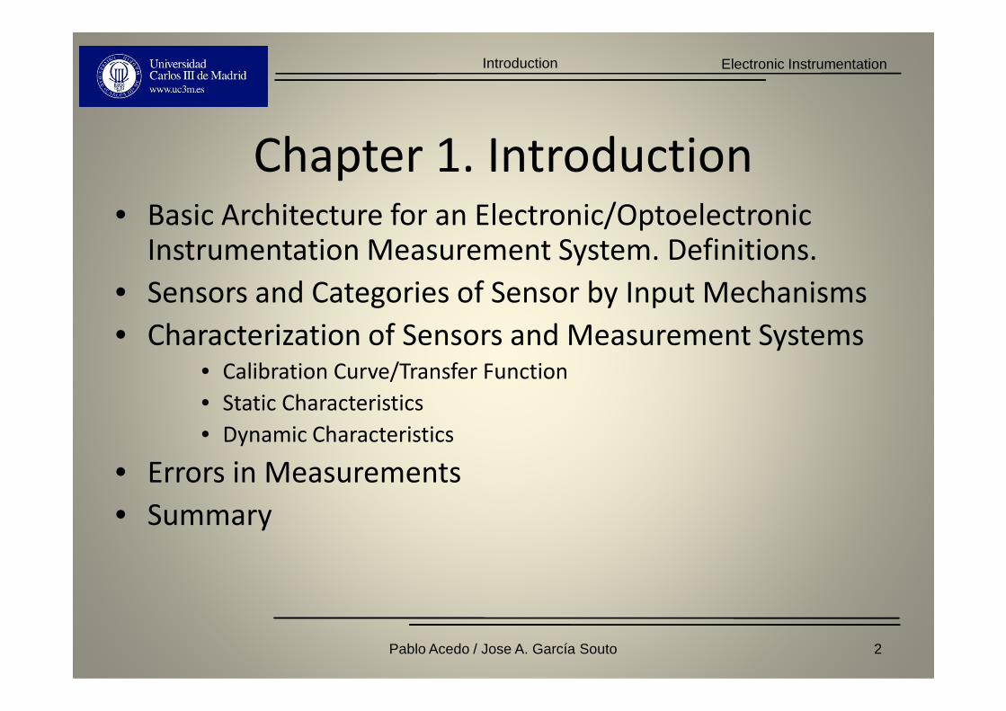
Chapter 1. Introduction• Basic Architecture for an Electronic/Optoelectronic
Instrumentation Measurement System. Definitions.
• Sensors and Categories of Sensor by Input Mechanisms
• Characterization of Sensors and Measurement Systems• Calibration Curve/Transfer Function
• Static Characteristics
• Dynamic Characteristics
• Errors in Measurements
• Summary
2Pablo Acedo / Jose A. García Souto
Electronic InstrumentationIntroduction
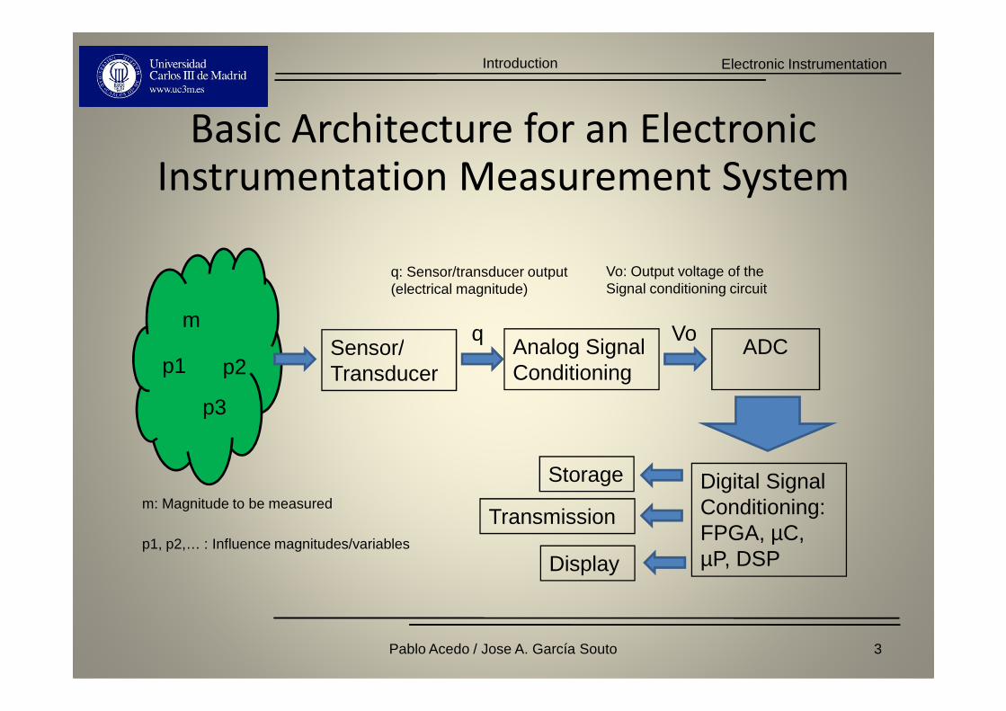
Basic Architecture for an Electronic Instrumentation Measurement System
Sensor/ Analog Signal m
p1 p2
q
q: Sensor/transducer output (electrical magnitude)
ADCVo
Vo: Output voltage of the Signal conditioning circuit
Sensor/Transducer
m: Magnitude to be measured
p1, p2,… : Influence magnitudes/variables
Analog Signal Conditioningp1 p2
p3
ADC
Digital Signal Conditioning: FPGA, µC, µP, DSPDisplay
Transmission
Storage
3Pablo Acedo / Jose A. García Souto
Electronic InstrumentationIntroduction
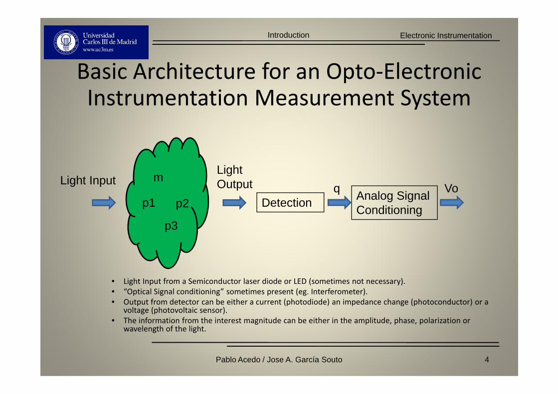
Basic Architecture for an Opto-Electronic Instrumentation Measurement System
m
p1 p2
Light InputLight Output
DetectionAnalog Signal
q Vop1 p2
p3
Detection
• Light Input from a Semiconductor laser diode or LED (sometimes not necessary).
• “Optical Signal conditioning” sometimes present (eg. Interferometer).
• Output from detector can be either a current (photodiode) an impedance change (photoconductor) or a voltage (photovoltaic sensor).
• The information from the interest magnitude can be either in the amplitude, phase, polarization or wavelength of the light.
Analog Signal Conditioning
4Pablo Acedo / Jose A. García Souto
Electronic InstrumentationIntroduction
Sensors
• There is always a form of energy conversion associated to the transduction
process.
A sensor is a device that receives a stimulus and responds with an electrical signal
process.
• A sensor can be a simple sensor or can be a complex system.
• Sensors can be classified in many ways depending on the criteria chosen:
• Field of applications
• Conversion Phenomena
• Specification
• Other
5Pablo Acedo / Jose A. García Souto

Electronic InstrumentationIntroduction
Categories of Sensor Input Mechanisms
• Resistive Sensors
• Variable Inductance/Magnetic Coupling
Sensors
• Capacitive Sensors
Passive Sensors
• Capacitive Sensors
• Voltage Generating Sensors
• Current Generating Sensors/optical Sensors
• Other Sensors
Active Sensors
6Pablo Acedo / Jose A. García Souto
Electronic InstrumentationIntroduction
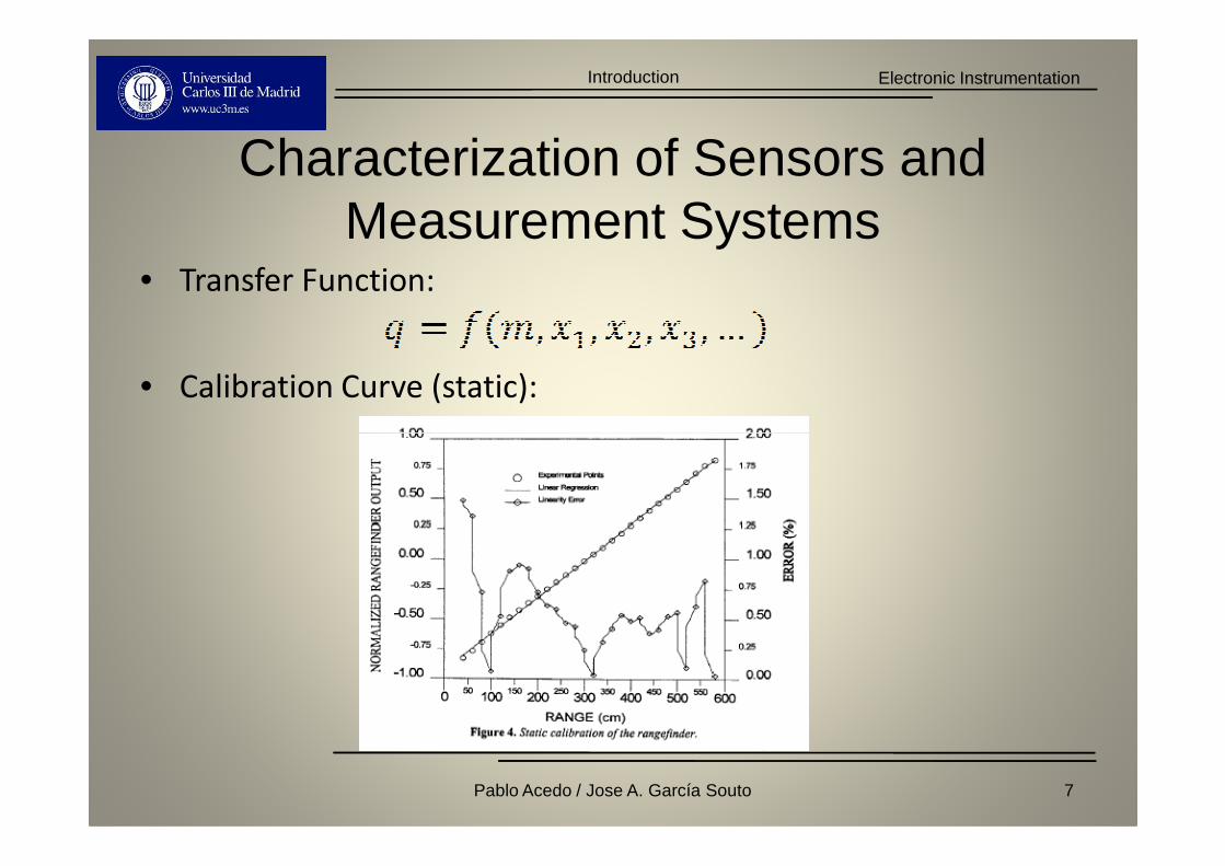
Characterization of Sensors and Measurement Systems
• Transfer Function:
• Calibration Curve (static):
7Pablo Acedo / Jose A. García Souto
Electronic InstrumentationIntroduction
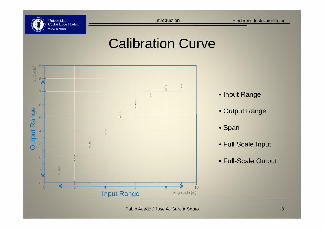
Calibration Curve
6
7
8
9
Out
put (
q)R
ange
• Input Range
• Output Range
0 2 4 6 8 10Magnitude (m)
0
1
2
3
4
5
Input Range
Out
put R
ange • Output Range
• Span
• Full Scale Input
• Full-Scale Output
8Pablo Acedo / Jose A. García Souto
Electronic InstrumentationIntroduction
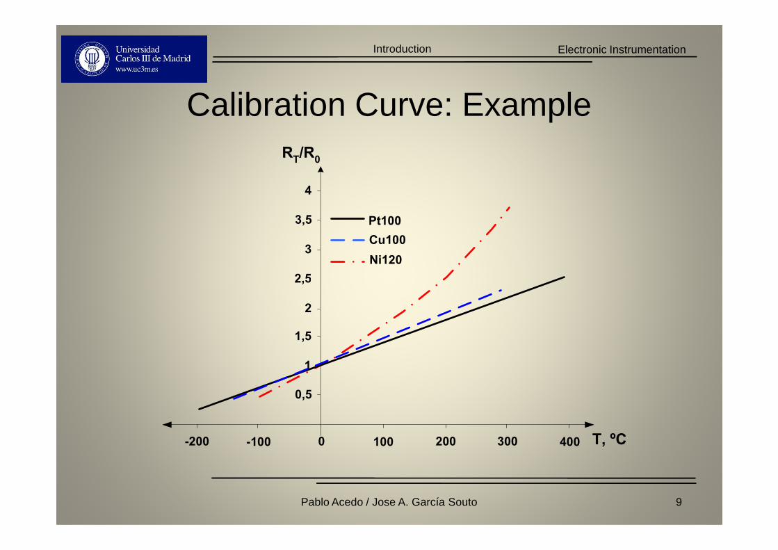
Calibration Curve: Example
2,5
3
3,5
4
RT/R
0
Pt100
Cu100
Ni120
9Pablo Acedo / Jose A. García Souto
0 100 200 300 400-100-200
0,5
1
1,5
2
2,5
T, ºC
Electronic InstrumentationIntroduction
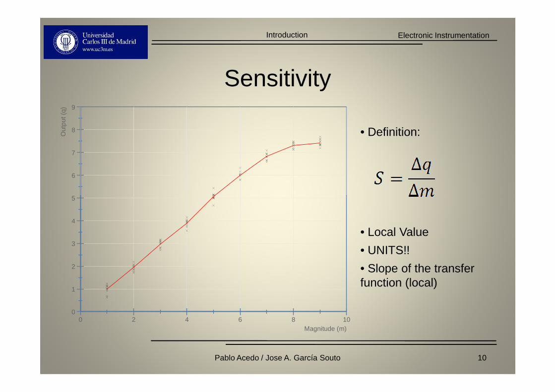
Sensitivity
5
6
7
8
9
Out
put (
q)
• Definition:
0 2 4 6 8 10Magnitude (m)
0
1
2
3
4
5
• Local Value
• UNITS!!
• Slope of the transfer function (local)
10Pablo Acedo / Jose A. García Souto
Electronic InstrumentationIntroduction
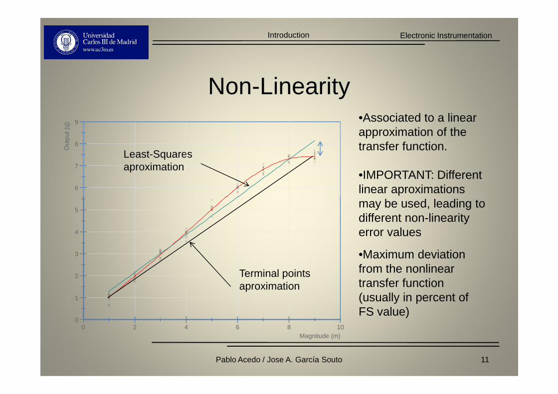
Non-Linearity
6
7
8
9
Out
put (
q)
•Associated to a linear approximation of the transfer function.
•IMPORTANT: Different linear aproximations may be used, leading to
Least-Squares aproximation
0 2 4 6 8 10Magnitude (m)
0
1
2
3
4
5may be used, leading to different non-linearity error values
•Maximum deviation from the nonlinear transfer function (usually in percent of FS value)
Terminal points aproximation
11Pablo Acedo / Jose A. García Souto
Electronic InstrumentationIntroduction
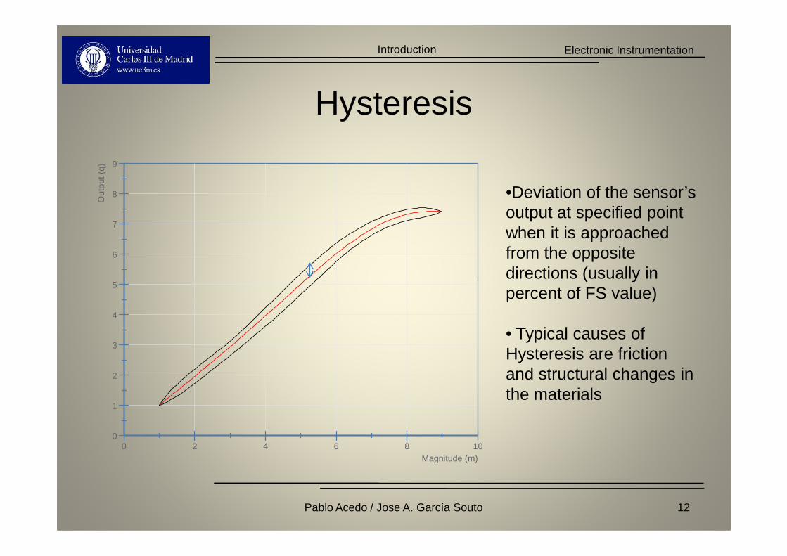
Hysteresis
•Deviation of the sensor’s output at specified point when it is approached from the opposite directions (usually in
6
7
8
9
Out
put (
q)
directions (usually in percent of FS value)
• Typical causes of Hysteresis are friction and structural changes in the materials
0 2 4 6 8 10Magnitude (m)
0
1
2
3
4
5
12Pablo Acedo / Jose A. García Souto

Electronic InstrumentationIntroduction
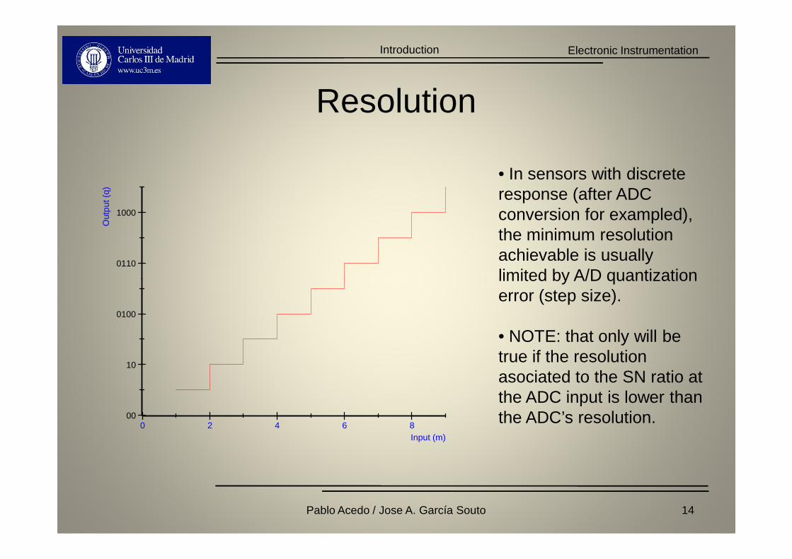
Resolution• Resolution: The smallest increment of the input that can be sensed.
0.4
0.6
0.8
0.4
0.6
0.8
• Important: For sensors with a continuous response some texts talk about infinitesimal resolution. That does not mean “infinite Resolution”.
0 200 400 600 800 1000-0.8
-0.6
-0.4
-0.2
0
0.2
time (ms)
Am
plitu
de (
mV
)
0 200 400 600 800 1000-0.8
-0.6
-0.4
-0.2
0
0.2
time (ms)
Am
plitu
de (
mV
)
Limited by the Signal-to-Noise ratio (S/N=0dB)
13Pablo Acedo / Jose A. García Souto
Electronic InstrumentationIntroduction
Resolution
0110
1000
Out
put (
q)
• In sensors with discrete response (after ADC conversion for exampled), the minimum resolution achievable is usually limited by A/D quantization
0 2 4 6 8Input (m)
00
10
0100
limited by A/D quantization error (step size).
• NOTE: that only will be true if the resolution asociated to the SN ratio at the ADC input is lower than the ADC’s resolution.
14Pablo Acedo / Jose A. García Souto

Electronic InstrumentationIntroduction
Precision/Accuracy
• Precision: consistency of the measurement. It is associated to the capacity of the sensor to give the same output (measurement) under 5
6
7
8
9
Out
put
(q)
output (measurement) under the same input (Stimulus).
• In modern sensors uncertainty is preferred asociated to the Limiting error of the measurement (to be discussed later)
0 2 4 6 8 10Magnitude (m)
0
1
2
3
4
5
15Pablo Acedo / Jose A. García Souto
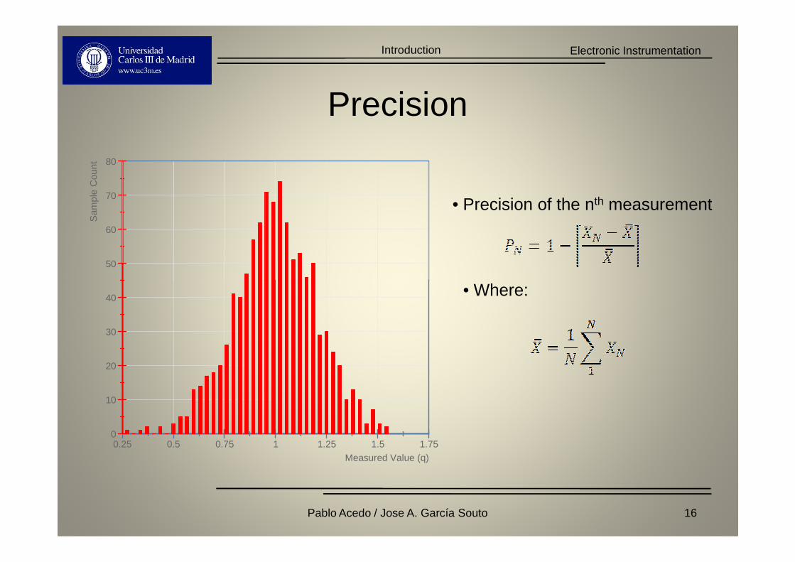
Electronic InstrumentationIntroduction
Precision
50
60
70
80
Sam
ple
Cou
nt
• Precision of the nth measurement
• Where:
0.25 0.5 0.75 1 1.25 1.5 1.75Measured Value (q)
0
10
20
30
40 • Where:
16Pablo Acedo / Jose A. García Souto
Electronic InstrumentationIntroduction
NOTE
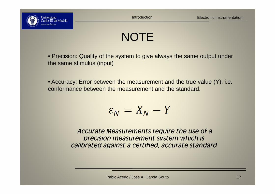
• Precision: Quality of the system to give always the same output under the same stimulus (input)
• Accuracy: Error between the measurement and the true value (Y): i.e. conformance between the measurement and the standard.
Accurate Measurements require the use of a Accurate Measurements require the use of a precision measurement system which is precision measurement system which is
calibrated against a certified, accurate standardcalibrated against a certified, accurate standard
17Pablo Acedo / Jose A. García Souto
Electronic InstrumentationIntroduction
Other Parameters
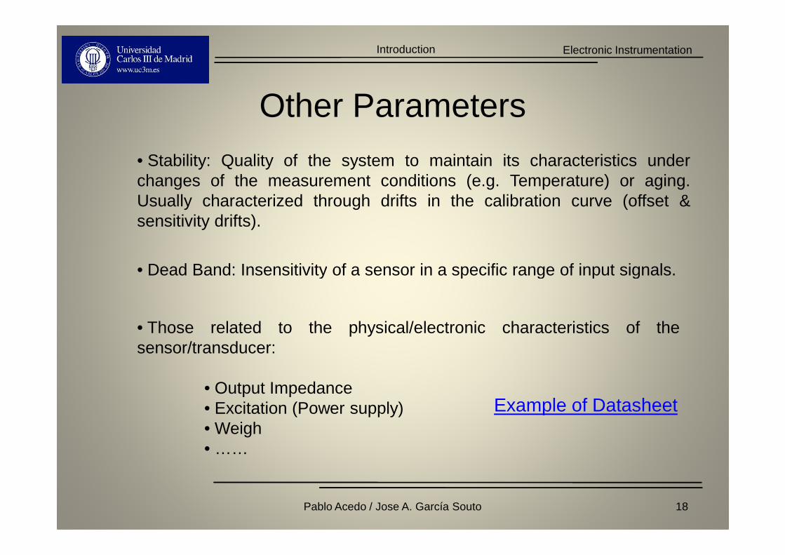
• Stability: Quality of the system to maintain its characteristics underchanges of the measurement conditions (e.g. Temperature) or aging.Usually characterized through drifts in the calibration curve (offset &sensitivity drifts).
• Dead Band: Insensitivity of a sensor in a specific range of input signals.• Dead Band: Insensitivity of a sensor in a specific range of input signals.
• Those related to the physical/electronic characteristics of thesensor/transducer:
• Output Impedance• Excitation (Power supply)• Weigh• ……
18Pablo Acedo / Jose A. García Souto
Example of Datasheet
Electronic InstrumentationIntroduction
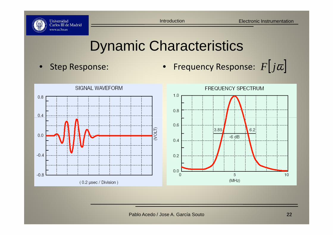
Dynamic Characteristics
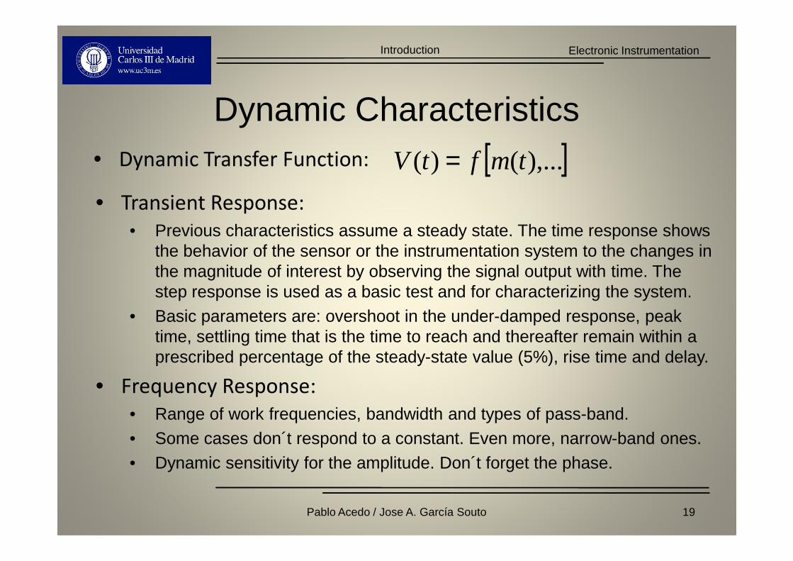
• Transient Response:
• Previous characteristics assume a steady state. The time response shows the behavior of the sensor or the instrumentation system to the changes in the magnitude of interest by observing the signal output with time. The
• Dynamic Transfer Function: [ ]),...()( tmftV =
the magnitude of interest by observing the signal output with time. The step response is used as a basic test and for characterizing the system.
• Basic parameters are: overshoot in the under-damped response, peak time, settling time that is the time to reach and thereafter remain within a prescribed percentage of the steady-state value (5%), rise time and delay.
• Frequency Response:
• Range of work frequencies, bandwidth and types of pass-band. • Some cases don´t respond to a constant. Even more, narrow-band ones.• Dynamic sensitivity for the amplitude. Don´t forget the phase.
19Pablo Acedo / Jose A. García Souto

Electronic InstrumentationIntroduction
Parameters of the time responseStep response
• Os: overshoot• ts: settling time
50%
Output response
Value 2100%
Error band (±ε)
Ostp
tr • ts: settling time• tr: rise time
t10-90
• td: delay• tp: peak time
50%
Magnitude of interest: analog step or discrete change
Value 10%
tdts
20Pablo Acedo / Jose A. García Souto
Electronic InstrumentationIntroduction
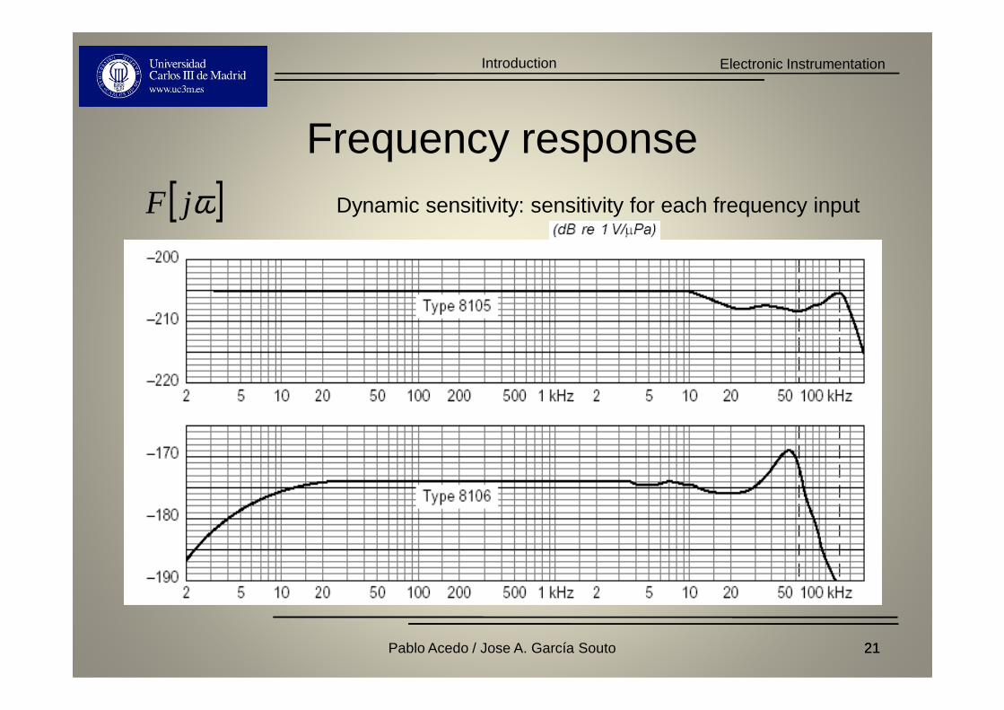
Frequency response[ ]ωjF Dynamic sensitivity: sensitivity for each frequency input
2121Pablo Acedo / Jose A. García Souto
Electronic InstrumentationIntroduction
Dynamic Characteristics• Step Response: • Frequency Response: [ ]ωjF
2222Pablo Acedo / Jose A. García Souto
Electronic InstrumentationIntroduction
Errors in Measurements
All measuring instruments should be regarded as guilty until proven innocent (P.K. Stein)
• Systematic Errors
• Random Errors (Noise/Interference)
• Gross Errors (Northrop)/Human Errors (Stein)
Sources/Classification of Errors
23Pablo Acedo / Jose A. García Souto
Electronic InstrumentationIntroduction
Limiting Error (LE)
Limiting Error (guarantee error) describes the Limiting Error (guarantee error) describes the outer bounds outer bounds of the expected of the expected worst caseworst case errorerror
• It includes all source of errors (gross/human errors
apart)apart)
• Value given by designer/manufacturers to specify
the precision (accuracy) of the instrument/sensor
• Related to uncertainty
24Pablo Acedo / Jose A. García Souto
Electronic InstrumentationIntroduction
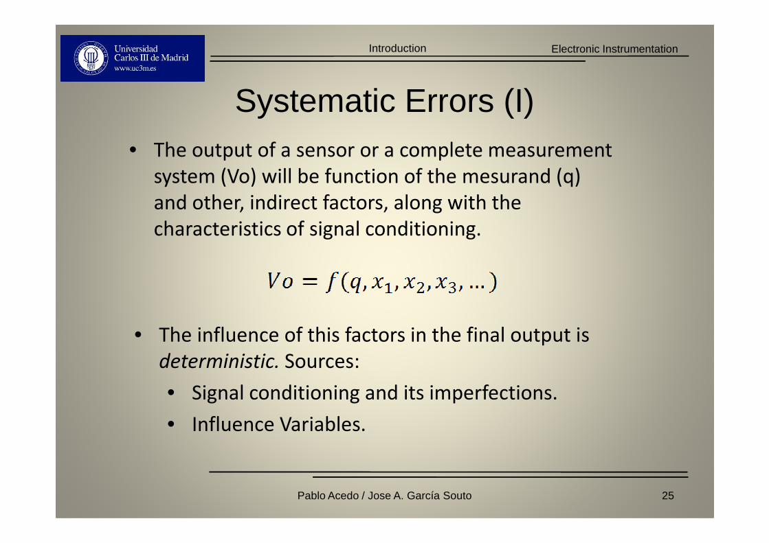
Systematic Errors (I)• The output of a sensor or a complete measurement
system (Vo) will be function of the mesurand (q)
and other, indirect factors, along with the
characteristics of signal conditioning.
• The influence of this factors in the final output is
deterministic. Sources:
• Signal conditioning and its imperfections.
• Influence Variables.
25Pablo Acedo / Jose A. García Souto

Electronic InstrumentationIntroduction
Propagation of Systematic Errors• As the influence of the different parameters is
deterministic, the combined effect of errors (∆xi)
using the linear error-propagation law using Taylor
series and removing all second and higher-order
terms.
• Usually is expressed in relative error.
26Pablo Acedo / Jose A. García Souto
Electronic InstrumentationIntroduction
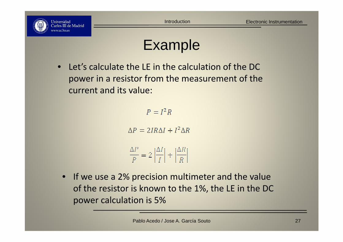
Example• Let’s calculate the LE in the calculation of the DC
power in a resistor from the measurement of the
current and its value:
• If we use a 2% precision multimeter and the value
of the resistor is known to the 1%, the LE in the DC
power calculation is 5%
27Pablo Acedo / Jose A. García Souto

Electronic InstrumentationIntroduction
Influence Variables• The output of the sensor is related not only to the
measurand value and the signal conditioning
(former example), but to other environmental
variables:
• Temperature•• Pressure
• Vibration
• ….
• The influence is also studied using the deterministic
linear error propagation law that allows also for
cancelation of effects (next chapter).
28Pablo Acedo / Jose A. García Souto
Electronic InstrumentationIntroduction
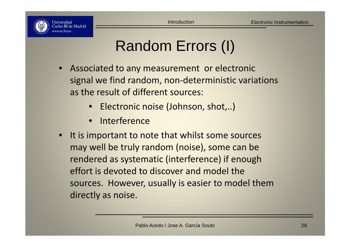
Random Errors (I)• Associated to any measurement or electronic
signal we find random, non-deterministic variations
as the result of different sources:
• Electronic noise (Johnson, shot,..)
• Interference• Interference
• It is important to note that whilst some sources
may well be truly random (noise), some can be
rendered as systematic (interference) if enough
effort is devoted to discover and model the
sources. However, usually is easier to model them
directly as noise.
29Pablo Acedo / Jose A. García Souto
Electronic InstrumentationIntroduction
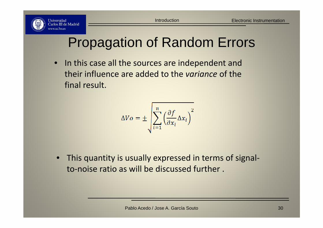
Propagation of Random Errors• In this case all the sources are independent and
their influence are added to the variance of the
final result.
• This quantity is usually expressed in terms of signal-
to-noise ratio as will be discussed further .
30Pablo Acedo / Jose A. García Souto
Electronic InstrumentationIntroduction
Gross/Human Errors
• Humans are always part of an instrument chain as
designers, manufacturers or observers.
• History is full of examples of errors due to wrong • History is full of examples of errors due to wrong
use of measurment units (SI vs Standard/Imperial)
• Instrumentation misuse, calculation errors and
other human mistakes are the main source of
wrong measurements!!!!
31Pablo Acedo / Jose A. García Souto
Electronic InstrumentationIntroduction
Summary
• The typical Architecture for an Electronic/Optoelectronic Instrumentation Measurement System has been presented, along with different sensor input mechanisms
• The Characterization of Sensors and Measurement Systems has been presented through the description of Systems has been presented through the description of the Static and Dynamic Characteristics from the Calibration Curve/Transfer Function
• Errors in Measurements have been also described and classified as something inherent to every measurement.
32Pablo Acedo / Jose A. García Souto


