OECD DEVELOPMENT CENTRE AE.pdf · determinants oecd development centre ... he opinions expressed...

MAKING DEVELOPMENT HAPPEN

Productive capabilities: An empirical investigation of their determinants

OECD DEVELOPMENT CENTRE

Christian Daude, Arne Nagengast and Jose Ramon Perea

Working Paper No. 321

Research area: Latin American Economic Outlook

December 2013

Productive Capabilities: An Empirical Investigation of their Determinants

DEV/DOC(2013)6

2 © OECD 2013

DEVELOPMENT CENTRE WORKING PAPERS

This series of working papers is intended to disseminate the Development Centre’s research findings rapidly among specialists in the field concerned. These papers are generally available in the original English or French, with a summary in the other language.

Comments on this paper would be welcome and should be sent to the OECD Development Centre, 2 rue André Pascal, 75775 PARIS CEDEX 16, France; or to [email protected]. Documents may be downloaded from: http://www.oecd.org/dev/wp or obtained via e-mail ([email protected]).

THE OPINIONS EXPRESSED AND ARGUMENTS EMPLOYED IN THIS DOCUMENT ARE THE SOLE RESPONSIBILITY OF THE AUTHORS AND

DO NOT NECESSARILY REFLECT THOSE OF THE OECD OR OF THE GOVERNMENTS OF ITS MEMBER COUNTRIES

©OECD (2013) Applications for permission to reproduce or translate all or part of this document should be sent to [email protected]

CENTRE DE DÉVELOPPEMENT DOCUMENTS DE TRAVAIL

Cette série de documents de travail a pour but de diffuser rapidement auprès des spécialistes dans les domaines concernés les résultats des travaux de recherche du Centre de développement. Ces documents ne sont disponibles que dans leur langue originale, anglais ou français ; un résumé du document est rédigé dans l’autre langue.

Tout commentaire relatif à ce document peut être adressé au Centre de développement de l’OCDE, 2 rue André Pascal, 75775 PARIS CEDEX 16, France; ou à [email protected]. Les documents peuvent être téléchargés à partir de: http://www.oecd.org/dev/wp ou obtenus via le mél ([email protected]).

LES IDÉES EXPRIMÉES ET LES ARGUMENTS AVANCÉS DANS CE DOCUMENT SONT CEUX DES AUTEURS ET NE REFLÈTENT PAS NÉCESSAIREMENT CEUX DE L’OCDE OU DES GOUVERNEMENTS DE SES PAYS MEMBRES

©OCDE (2013) Les demandes d'autorisation de reproduction ou de traduction de tout ou partie de ce document devront être envoyées à [email protected]

OECD Development Centre Working Paper No.321

DEV/DOC(2013)6

© OECD 2013 3

TABLE OF CONTENTS

ACKNOWLEDGEMENTS .......................................................................................................................... 4

PREFACE ....................................................................................................................................................... 5

RÉSUMÉ ........................................................................................................................................................ 6

ABSTRACT .................................................................................................................................................... 6

I. INTRODUCTION ..................................................................................................................................... 7

II. METHODS AND EMPIRICAL STRATEGY ...................................................................................... 10

III. RESULTS ................................................................................................................................................ 18

IV. CONCLUSION ..................................................................................................................................... 25

ANNEX ........................................................................................................................................................ 27

REFERENCES ............................................................................................................................................. 32

OTHER TITLES IN THE SERIES/ AUTRES TITRES DANS LA SÉRIE .............................................. 35


DEV/DOC(2013)6

4 © OECD 2013

ACKNOWLEDGEMENTS

The authors would like to thank Jake Schurmeier for his capable research assistance and René Orozco who helped editing the paper. All remaining errors are the authors’ responsibility.


DEV/DOC(2013)6

© OECD 2013 5

PREFACE

Economic development requires an eventual change in productive specialisation. This process, known as structural transformation, refers to the reallocation of economic activity across broad economic sectors, and specifically away from agriculture. Recent research has associated structural transformation, and ultimately development, to a change in the type of goods a country produces and exports. This change entails a gradual move towards goods that embody greater physical and/or human capital. Thus, this line of work has also been able to create a variable that embodies the “economic complexity” of a country, otherwise a proxy for the productive capabilities of an economy.

This paper focuses on unveiling the determinants of this variable. In line with the breadth of the related literature, there is a large set of factors that can potentially affect the degree of economic complexity of a country. This, in turn, heightens the uncertainty in selecting the adequate empirical model that explains the behaviour of our dependent variable most accurately. To address this challenge, the paper adopts an econometric methodology that considers all possible combinations of specifications, across a broad set of potential regressors.

The analysis singles out a few variables that are significantly associated with economic complexity. This is the case, for instance, of commodity terms of trade, energy availability, government consumption, capital per worker, arable land or the accrual of capital flows. An identification we deem relevant, not only because of the exhaustive empirical investigation to which these variables have been subjected to; but also because some of them are susceptible to policy intervention.

This work contributes to the OECD Development Centre’s interest to disentangle a more accurate account of which factors, and therefore which policies, facilitate and sustain development. In this way, I hope it will provide valuable guidance on an issue that remains of critical importance for many countries.

Mario Pezzini Director

OECD Development Centre December 2013


DEV/DOC(2013)6

6 © OECD 2013

RÉSUMÉ

Les contributions récentes à la littérature sur la croissance économique ont fait valoir que la structure d'une économie, mesurée par ses capacités de production, est un facteur déterminant pour les différences de développement inter-pays. Les capacités productives sont considérées être hautement prédictives de la croissance économique future, mais leurs déterminants au niveau des pays sont restés inconnus. Dans cet article, nous explorons empiriquement les déterminants à l'aide d'un cadre d'étalement du modèle qui peut gérer un très grand nombre de variables explicatives, sans la nécessité d'une sélection de modèle. Afin d'estimer notre spécification de panel dynamique, nous proposons un nouveau calcul de la procédure de moyenne bayésienne d’estimation classique basé sur l'estimateur simple et efficace corrigé par un estimateur à effets fixes. Notre référence et analyse de robustesse considèrent un grand nombre de variables, périodes d'échantillonnage et prieurs de modèle. Nous constatons que le stock existant de capacités (mesuré par la variable dépendante retardée), les termes de l’échange sur les matières premières, la disponibilité de l’énergie, la consommation publique, le capital par travailleur, les terres arables et les flux de capitaux montrent une association importante et robuste sur les capacités.

ABSTRACT

Recent contributions to the growth literature have argued that the structure of an economy, as measured by its productive capabilities, is a key determinant for inter-country differences in development. Productive capabilities have been shown to be highly predictive of future economic growth, yet their country-level determinants have remained unknown. In this paper, we empirically explore their determinants using a model averaging framework that can handle a very large number of explanatory variables without the need for model selection. In order to estimate our dynamic panel specification, we propose a novel Bayesian Averaging of Classical Estimates procedure based on the simple and efficient bias-corrected LSDV estimator. Our baseline and robustness analysis consider a large number of variables, sample periods and model priors. We find that the existing stock of capabilities (as measured by the lagged dependent variable), commodity terms of trade, energy availability, government consumption, capital per worker, arable land and capital inflows show a strong and robust association with capabilities.

JEL Classification: C11; O11; O14; O33; F43 Keywords: capabilities; economic complexity; exports; growth; Bayesian model averaging.


DEV/DOC(2013)6

© OECD 2013 7

I. INTRODUCTION

Development economists have often argued that the type and range of goods that a country produces and exports is at the core of structural transformation, and ultimately economic development. In essence, economic development is often defined as the transition of production factors from traditional activities, largely in agriculture towards value creation embodying greater physical and human capital (Kuznets, 1955 ; Kaldor ,1963). A major part of the literature has focused on the special role of the abundance of natural resources in developing economies. Primary commodities have been argued to lead to deteriorating terms of trade for natural resource countries (Prebisch, 1950), greater volatility in export revenues (Easterly and Kraay, 2000), Dutch disease (Corden, 1982), and poor institutional quality (Sachs and Warner, 1995; Ross, 2001; Collier and Hoeffler, 2005). More recent research has shifted the focus from differences in sector shares to differences in product characteristics. Accordingly, the process of structural transformation involves a change in the type of goods that are produced, i.e. shifting production from simple to complex or sophisticated goods (Lall, 2000; Hausmann and Klinger, 2006; Hausmann et al., 2007). In this literature, what a country produces is indicative of its developmental stage, with advanced economies generally producing and exporting high-technology and high-skill products. In a recent contribution to this literature, Hidalgo and Hausmann (2009) propose a network theoretic measure of the productive capabilities of an economy based purely on trade data. They do so using the “method of reflections”, which combines the level of export diversification of a country and the average ubiquity of the goods it exports using a bipartite network algorithm. The rationale behind this approach is that countries that export a large range of products (i.e. are highly diversified) are likely to have more capabilities. Similarly, products that are exported by relatively few countries (i.e. products with low ubiquity) seem to require many of hard-to-find capabilities. Hidalgo and Hausmann (2009) show that after controlling for initial levels of development the capabilities measure is highly predictive of future economic growth.1 This work has attracted considerable interest in the literature and international development institutions (Jankowska et al., 2012; Lederman & Maloney, 2012; UNESCAP, 2011 and many others). If capabilities play such an important role for economic growth, it is crucial to understand the process of capability formation. Hausmann and Hidalgo (2011) build a theoretical model that

1 See also Ourens (2013) for a use of alternative data sources and several robustness checks of this finding.


DEV/DOC(2013)6

8 © OECD 2013

features strong path dependence in capability accumulation, which they define as the quiescence trap. Since many products require the combination of several capabilities, countries with few capabilities will have a lower probability of finding alternative uses for any additional capability than countries having a large pool of capabilities. In this way, countries with low capabilities will have lower incentives to accumulate additional capabilities. According to the authors, this trap helps to explain the persistent differential in income levels between countries, since initial differences in capability endowments would be amplified overtime.

The way the relationship between a country’s export profile and development is portrayed in the literature on capabilities also suggests a very specific set of policy recommendations, in particular with regards to industrial policies. According to Hausmann et al. (2011) countries should follow a targeted diversification strategy that favours expansion into more sophisticated activities and aim to increase the number of exported products according to two criteria. First, selecting those which are most sophisticated and hence promise the greatest increase in the country’s capabilities. Second, choosing them according to their proximity, i.e. the match with existing capabilities. All things considered, the literature on capabilities arrives at an interesting crossroad, which motivates our study. On the one hand, the analysis draws bold conclusions about the link between the theoretical construct of capabilities and economic development, some of which depart substantially from conventional trade theory. Yet, this contrasts with the ambiguity that still surrounds the definition of capabilities: Hidalgo and Hausmann (2009) describe capabilities as those requirements that are necessary for producing a certain set of goods and are essentially non-tradeable. Generally, these would include a wide range of factors such as aspects of governance (e.g. rule of law, property rights), the level of infrastructure, and the skill endowment of the labour force. The vice and virtue of the computation of the capabilities variable is that the method of reflections only requires international trade data as input. In doing so, it effectively circumvents the question of which country-level determinants account for the level of capabilities. The lack of clarity on the determinants of capabilities also has ramifications for policy recommendations. If capabilities can be improved by exporting more sophisticated goods, the main policy advice that results is a targeted support of industries based on the sophistication of their products, and their proximity to the current set of capabilities. Even though it is reasonable to assume that the products a country exports without market intervention are a measure of their productive capabilities, to start exporting a particular good at any cost because of the above considerations might not necessarily improve the capabilities of that country. This will be particularly true if structural factors such as the market structure, the factor endowments and infrastructure of a country are not favourable for producing and exporting that particular good. However, if the country-level determinants of capabilities were known an alternative course of action would be the improvement of a particular set of structural variables (e.g. education, infrastructure, business environment, etc.) that can be seen as conducive to the accumulation of


DEV/DOC(2013)6

© OECD 2013 9

capabilities, which would then facilitate the inception and growth of more sophisticated industries. Our study aims to shed light on the determinants of capabilities through an empirical analysis that considers a broad set of potential variables. These encompass institutional, macroeconomic, skill-related, and other “non-tradeable” features of an economy, as suggested in Hidalgo and Hausmann (2009). Specifically, the set of variables we consider can be grouped into different categories related to macroeconomic conditions, financial development, economic structure, external sector, demographics, education and skills, infrastructure and importance of the primary sector. In all, this comprehensive approach allows us to combine variables where the room for policy influence is more evident, as would be case for a variable such as the fiscal deficit; to those that are relatively unaffected by policy, either for being structural in nature (e.g. demography), or for being partially dependent on external factors (e.g. terms of trade). Consequently, the extent to which the policymaking process can influence the capabilities endowments of a country will largely depend on which type of determinant turns out to be more important. The consideration of a large set of potential explanatory variables requires a robust estimation procedure, for which Bayesian Model Averaging (BMA) is the method of choice. As we will see below, BMA is well-suited to account for the uncertainty associated with model selection, a feature that gains importance in empirical specifications that consider many explanatory variables. In our setting, it is desirable to use a fixed effects specification to account for unobserved heterogeneity across countries. Due to the persistence of the capabilities measure over time, this variable needs to be included in lags in the estimation equations. However, the lagged dependent variable in the presence of country-fixed effects leads to the well-known Nickel bias of the least squares dummy variable (LSDV) estimator (Nerlove, 1971; Nickell, 1981). Here, we develop a new BMA procedure based on the simple and efficient bias corrected LSDV estimator Kiviet (1995, 1999) to estimate the dynamic panel specification. The remainder of the paper proceeds as follows. Section II details the construction of the measure on capabilities, as defined in Hidalgo and Haussmann (2009); it describes the BMA methodology and introduces of the bias-corrected LSDV estimator into the BMA framework. Section III discusses the results and their robustness, and section IV concludes.


DEV/DOC(2013)6

10 © OECD 2013

II. METHODS AND EMPIRICAL STRATEGY

In this section, we present in detail how the capabilities variable used as dependent variable in our analysis is constructed. Second, we discuss in detail the Bayesian model averaging approach used in this study, as well as our preferred estimator, the priors and computational implementation. Finally, we introduce the definitions and sources of the explanatory variables included in the empirical analysis.

Capabilities measure

The capabilities measure proposed by Hidalgo and Hausmann (2009) is based on an algorithm that combines information of the diversification of a country and the ubiquity of the products it exports. Whether a country is effectively exporting a good is assessed by its revealed comparative advantage 𝑅𝐶𝐴𝑐𝑝 following Balassa (1965) as the ratio of the export share 𝑥𝑐𝑝 of product 𝑝 in country 𝑐 to the export share of product 𝑝 in world trade

𝑅𝐶𝐴𝑐𝑝 =𝑥𝑐𝑝 ∑ 𝑥𝑐𝑝𝑝⁄

∑ 𝑥𝑐𝑝𝑐 ∑ ∑ 𝑥𝑐𝑝𝑝𝑐⁄

A country is assumed to be competitive in exporting a product 𝑝 if its revealed comparative advantage (𝑅𝐶𝐴𝑐𝑝) is greater than 1, i.e. if the share of product 𝑝 in country 𝑐’s export basket is greater than the share of the same good globally. Therefore, we can define the following indicator function for country 𝑐 having a comparative advantage in product 𝑝 as:

|𝑅𝐶𝐴|𝑐𝑝= � 0 if 𝑅𝐶𝐴𝑐𝑝<1 1 if 𝑅𝐶𝐴𝑐𝑝≥1

The observed level of diversification 𝐾𝑐,0 of a country 𝑐 is then defined as the number of products in which the country has a revealed comparative advantage. Conversely, the ubiquity 𝐾𝑝,0 of a product 𝑝 is defined as the number of countries exporting that product with a revealed comparative advantage:

𝐾𝑐,0 = �|𝑅𝐶𝐴|𝑐𝑝𝑝


DEV/DOC(2013)6

© OECD 2013 11

𝐾𝑝,0 = �|𝑅𝐶𝐴|𝑐𝑝𝑐

Next, these two indicators are combined using a bipartite network representation of countries and products, in which countries and products are connected if a country has a revealed comparative advantage greater than one in that particular product category

𝐾𝑐,𝑁 =1

𝐾𝑐,0�|𝑅𝐶𝐴|𝑐𝑝𝐾𝑝,𝑁−1

𝑝

𝐾𝑝,𝑁 =1

𝐾𝑝,0�|𝑅𝐶𝐴|𝑐𝑝𝐾𝑐,𝑁−1

𝑐

where 𝐾𝑐,𝑁 is the 𝑁th country moment and 𝐾𝑝,𝑁 is the 𝑁th moment on the product side. Iterating the equations for 𝐾𝑐,𝑁 and 𝐾𝑝,𝑁 gradually extracts more information about product sophistication, on the product side, and capabilities, on the country side, and this procedure was iterated until convergence. Then, the capabilities measure was computed based on a sample of 103 countries for which data for the entire time period from 1976-2010 is available. The actual value of the measure is sensitive to the overall connectivity in the network, which changes over time, and hence comparisons across years are only meaningful if the measure is standardised across countries for each year:

𝑐𝑎𝑝𝑎𝑏𝑐 =𝐾𝑐,∞ − 𝐸(𝐾𝑐,∞)

�𝑉𝑎𝑟(𝐾𝑐,∞),

where time subscripts have been omitted to simplify notation. A value of zero in this measure corresponds to a country having the same capabilities as the world average; a value of one corresponds to a country that is one standard deviation above world average. When observing changes over time in this measure, one can determine whether a country has improved its position relative to other countries, while of course it is likely that on average all countries have improved their capabilities over time. The standardisation of the capabilities measure has consequences for our statistical analysis. Since the dependent variable is by definition a relative measure, the actual levels of the explanatory variables are not meaningful and only changes in their values relative to other countries are of importance. Hence, all the independent variables are standardised accordingly for a given cross-section of the panel. This is equivalent to running a regression with standardised coefficients. Therefore, the coefficients are to be interpreted as how many standard deviations the dependent variable changes for a standard deviation increase in the explanatory variables.


DEV/DOC(2013)6

12 © OECD 2013

Bayesian model averaging

As discussed in the introduction, a large number of variables could in principle determine the productive capabilities of a country. If the number of explanatory variables (𝐾) is substantially smaller than the number of observations (𝑁), a simple regression could be run to identify the most important determinants. However, if 𝐾 is close to 𝑁, statistical estimates become too imprecise to yield robust and meaningful results. A popular approach in the growth literature to overcome this problem has been to use Bayesian model averaging (Fernández et al., 2001; Sala-i-Martin et al., 2004; Ciccone and Jarocinski, 2010; Moral-Benito, 2012). Bayesian model averaging focuses on the fact that there is substantial model uncertainty, i.e. that it is not clear which model out of the many possible specifications given a set of 𝐾 explanatory variable has generated the data. Model uncertainty is accounted for by estimating all possible models and by evaluating the probability of each model given the data. Subsequently, the (posterior) model probability can be used to calculate a proxy for the importance of a variable (the posterior inclusion probability) and for calculating weighted averages of the mean and variance of the coefficients. Formally, there are 𝑗 = 1, … ,2𝐾 different models formed by all combinations of the 𝐾 explanatory variables. For a given model 𝑀𝑗 with a subset of independent variables 𝑥𝑗 consider the panel regression of the form

𝑦𝑖𝑡 = 𝑥𝑖𝑡𝑗 𝛽𝑗 + 𝜀𝑖𝑡

𝑗 where 𝑦𝑖𝑡 is the capabilities measure of country 𝑖 in time period 𝑡, 𝛽𝑗 are the marginal effects of the explanatory variables included in the model and 𝜀𝑖𝑡

𝑗 is an error term. In this article, we use Bayesian model averaging of classical estimates following Raftery (1995) and Sala-i-Martin et al. (2004), for which standard econometric methods can be used to estimate this equation. A key statistic in the model averaging framework is the posterior model probability 𝑃�𝑀𝑗�𝑦� of model 𝑀𝑗. We follow Raftery (1995) in using the Schwarz asymptotic approximation to the integrated likelihood which in a panel context is given by

𝑃�𝑀𝑗�𝑦� =𝑃�𝑀𝑗�(𝑁𝑇)−𝑘𝑗 2⁄ 𝑆𝑆𝐸𝑗

−(𝑁𝑇) 2⁄

∑ 𝑃(𝑀𝑖)(𝑁𝑇)−𝑘𝑖 2⁄ 𝑆𝑆𝐸𝑖−(𝑁𝑇) 2⁄2𝐾

𝑖

where 𝑃�𝑀𝑗� is the prior model probability, 𝑁𝑇 is the number of observations (𝑁 is the cross-section and 𝑇 the time dimension), 𝑘𝑗 is the number of parameters included in the model and 𝑆𝑆𝐸𝑗 is the sum of squared residuals of model regression 𝑗. Note that the posterior model probability comprises the degrees of freedom adjustment (𝑁𝑇)−𝑘𝑗 2⁄ , as information criteria do, independent of the prior. An important summary statistic is the posterior inclusion probability (PIP), which is a proxy for the importance of a variable in explaining changes in the dependent variable. The PIP of explanatory variable 𝑘 is given by the sum of the posterior probabilities of all models in which the variables was included:


DEV/DOC(2013)6

© OECD 2013 13

𝑃𝐼𝑃𝑘 = 𝑃(𝜃𝑘 ≠ 0|𝑦) = � 𝑃�𝑀𝑗�𝑦�𝜃𝑘≠0

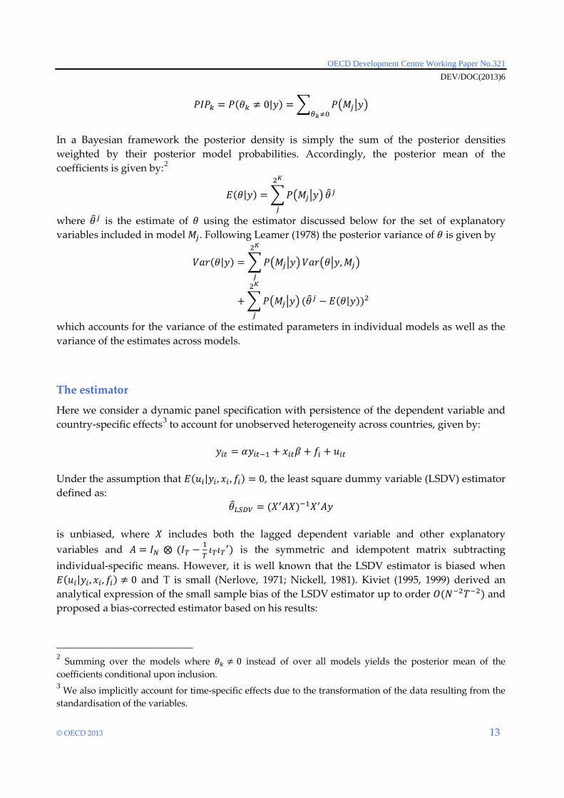
In a Bayesian framework the posterior density is simply the sum of the posterior densities weighted by their posterior model probabilities. Accordingly, the posterior mean of the coefficients is given by:2

𝐸(𝜃|𝑦) = � 𝑃�𝑀𝑗�𝑦�2𝐾

𝑗

𝜃�𝑗

where 𝜃�𝑗 is the estimate of 𝜃 using the estimator discussed below for the set of explanatory variables included in model 𝑀𝑗. Following Leamer (1978) the posterior variance of 𝜃 is given by

𝑉𝑎𝑟(𝜃|𝑦) = � 𝑃�𝑀𝑗�𝑦�2𝐾

𝑗

𝑉𝑎𝑟�𝜃�𝑦, 𝑀𝑗�

+ � 𝑃�𝑀𝑗�𝑦�2𝐾

𝑗

(𝜃�𝑗 − 𝐸(𝜃|𝑦))2

which accounts for the variance of the estimated parameters in individual models as well as the variance of the estimates across models.

The estimator

Here we consider a dynamic panel specification with persistence of the dependent variable and country-specific effects3 to account for unobserved heterogeneity across countries, given by:

𝑦𝑖𝑡 = 𝛼𝑦𝑖𝑡−1 + 𝑥𝑖𝑡𝛽 + 𝑓𝑖 + 𝑢𝑖𝑡 Under the assumption that 𝐸(𝑢𝑖|𝑦𝑖 , 𝑥𝑖 , 𝑓𝑖) = 0, the least square dummy variable (LSDV) estimator defined as:

𝜃�𝐿𝑆𝐷𝑉 = (𝑋′𝐴𝑋)−1𝑋′𝐴𝑦 is unbiased, where 𝑋 includes both the lagged dependent variable and other explanatory variables and 𝐴 = 𝐼𝑁 ⨂ (𝐼𝑇 − 1

𝑇𝜄𝑇𝜄𝑇

′) is the symmetric and idempotent matrix subtracting individual-specific means. However, it is well known that the LSDV estimator is biased when 𝐸(𝑢𝑖|𝑦𝑖 , 𝑥𝑖, 𝑓𝑖) ≠ 0 and T is small (Nerlove, 1971; Nickell, 1981). Kiviet (1995, 1999) derived an analytical expression of the small sample bias of the LSDV estimator up to order 𝑂(𝑁−2𝑇−2) and proposed a bias-corrected estimator based on his results:

2 Summing over the models where 𝜃𝑘 ≠ 0 instead of over all models yields the posterior mean of the coefficients conditional upon inclusion. 3 We also implicitly account for time-specific effects due to the transformation of the data resulting from the standardisation of the variables.


DEV/DOC(2013)6

14 © OECD 2013

𝜃�𝐿𝑆𝐷𝑉𝐶 = 𝜃�𝐿𝑆𝐷𝑉 − 𝐸(𝜃�𝐿𝑆𝐷𝑉 − 𝜃) The bias corrected LSDV estimator (LSDVC) generally has been shown to be a more efficient estimator than alternative IV and GMM-estimators that also address the bias arising from the lagged dependent variable (Anderson and Hsiao, 1981; Arellano and Bond, 1991). For example, Judson and Owen (1999) use Monte Carlo simulations to show that for panels of all sizes the bias corrected estimator consistently has the lowest root mean squared error in comparison to OLS, Anderson-Hsiao and GMM estimators. Moral-Benito (2012) proposes a maximum likelihood estimator whose first moment conditions correspond to those of the GMM problem to deal with the endogeneity of the lagged dependent variable in a Bayesian model averaging context. However, the small-sample properties of this estimator have so far not been investigated. Hence, in this study we combine the estimates of the LSDVC estimator using the model averaging framework outline above. In the robustness analysis, we show that the model averaging results of the LSDV and the LSDVC estimator differ appreciably from each other and that the bias of the LSDV estimator for our dataset is not negligible.

The prior

We use the relatively standard binomial distribution over the model size Κ as a prior distribution (Sala-i-Martin et al., 2004):

Κ~𝐵𝑖𝑛(𝐾, 𝜑)

𝐸(Κ) = 𝐾𝜑 = 𝐾𝑘�𝐾

= 𝑘�

where 𝜑 = 𝑘� 𝐾⁄ is the prior inclusion probability of each variable and 𝑘� is the prior expected model size. In this framework, the prior model probability of model 𝑀𝑗 with 𝑘𝑗 different explanatory variables is

𝑃�𝑀𝑗� = (𝜑)𝑘𝑗(1 − 𝜑)𝐾−𝑘𝑗 . This specification only requires the choice of the prior expected model size, which we set to 𝑘� = 10. This is slightly larger than in previous studies on the determinants of growth in cross-section regressions with 𝑘� = 7 (Sala-i-Martin et al., 2004) and in the panel setting with 𝑘� = 5 (Moral-Benito, 2012). However, as there is currently little prior knowledge on the determinants of productive capabilities and the measure has potentially many determinants we chose a slightly larger expected model size as a reflection of this uncertainty. We investigate the robustness of our results to our prior assumptions in two ways. First, we examine the effect of the prior expected model size of the binomial prior on our results. In the alternative specification 𝑘� is set to 5 and 15. Second, we use a random rather than a fixed prior specification. Using a fixed 𝜑 prior has been criticised by Ley and Steel (2009) on the grounds that the results are more sensitive to the choice of the prior expected model size parameter 𝑘� than


DEV/DOC(2013)6

© OECD 2013 15

alternative hierarchical prior specifications which allow 𝜑 to be random. To address this issues, Ley and Steel (2009) propose the use of a beta-binomial prior over the model size Κ

Κ~𝐵𝑖𝑛(𝐾, 𝜑) 𝜑~𝐵𝑒𝑡𝑎(𝑎, 𝑏),

where 𝑎, 𝑏 > 0 are hyperparameters and 𝜑 is now a probabilistic variable that is drawn from a beta distribution. The prior expected model size in this framework is

𝐸(Κ) =𝑎

𝑎 + 𝑏𝐾.

Ley and Steel (2009) propose a choice of 𝑎 = 1 and 𝑏 = (𝐾 − 𝑘�) 𝑘�⁄ , which allows setting the prior expected model size as in the case of the binomial prior and hence makes the results directly comparable. In our robustness analysis, we set 𝑘� = {5,10,15} to compare the results with those of the fixed binomial prior specification.

Computational implementation

The number of models that has to be evaluated grows exponentially with the number of covariates included in the regression. A complete evaluation of all models with 𝐾 covariates would require running 2𝐾 regressions. For 𝐾 = 30, this is equivalent to 1.07 ∙ 109 model evaluations, which is computationally infeasible. As a solution, algorithms have been developed which carry out Bayesian model averaging without the need for evaluating every possible model (Koop, 2003). Here, we employ the commonly used Markov Chain Monte Carlo Model Composition (MC3) algorithm originally proposed by Madigan, York and Allard (1995). The MC3 constructs a Markov Chain in model space whose stationary distribution converges to the posterior model probability distribution by sampling from regions in model space where the posterior model probability is high. Specifically, the MC3 simulates a chain of models 𝑀(𝑠) for 𝑠 = 1, … , 𝑆 samples where 𝑀(𝑠) is sampled from the set of all possible models {𝑀1, … , 𝑀2𝐾}. The birth-and-death sampler is used to implement the MC3, in which the candidate model 𝑀(𝑠) is identical to the current model 𝑀(𝑠−1) except for one variable. In each iteration, one of the 𝐾 covariates is drawn at random. If the explanatory variable already forms part of the current model 𝑀(𝑠−1), then the variable is deleted in the candidate model 𝑀(𝑠). Similarly, if the drawn explanatory variable is not included in the current model, then it is added in the candidate model. The posterior model probability for the candidate model is computed and the proposal is accepted with probability:

min{𝑃�𝑀(𝑠)�𝑦�

𝑃(𝑀(𝑠−1)|𝑦) , 1}.

If the candidate model is not accepted, then the Markov Chain remains at the current model (𝑀(𝑠) = 𝑀(𝑠−1)). The algorithm was run until convergence, which was verified by the correlation


DEV/DOC(2013)6

16 © OECD 2013

coefficient between the relative frequencies of model visits and the analytical posterior model probabilities for the 10 000 best models (Fernández, Ley and Steel, 2001).

Data

Our data sample is conditioned by the need to incorporate a comprehensive set of variables, representative of all the dimensions that could potentially affect capabilities.4 While a more complete definition of the variables and their sources is included in the appendix, here we simply list the variables used in the baseline specification, along the following thematic classification. - Macroeconomic conditions: GDP volatility, GDP growth, current account balance, government consumption over GDP, inflation, total reserves over GDP, currency overvaluation. - Financial Development: money and quasi-money as percentage of GDP, domestic credit over GDP. - Physical capital: capital per worker, gross capital formation over GDP. - External sector: Trade openness, capital account openness, foreign direct investment over GDP, capital flows over GDP, terms of trade. - Demographics: population, population growth, age dependency ratio, life expectancy. - Education/Skills: average years of schooling, percentage of population with secondary education, percentage of population with tertiary education. - Infrastructure: number of telephone lines per 100 people, energy use, energy production, - Importance of primary sector: agricultural land as percentage of total land, arable land as percentage of total land. The implementation of BMA requires having a balanced panel, a condition that significantly reduces the number of countries for which the previous variables are available. This condition leaves our baseline specification with 43 countries, listed below according to latest 2012 World Bank’s income group classification.5

4 The rationale for the different groups of variables is discussed in the introduction. 5 See http://data.worldbank.org/news/new-country-classifications for details.

http://data.worldbank.org/news/new-country-classifications


DEV/DOC(2013)6

© OECD 2013 17

Lower middle income Upper middle income High income

Bolivia, Cote d’Ivoire, Cameroon, Egypt, Ghana, Guatemala, Honduras, Sri Lanka, Morocco, Pakistan, Philippines, Paraguay, Senegal, El Salvador.

Colombia, Costa Rica, Dominican Republic, Ecuador, Jamaica, Jordan, Mexico, Malaysia, Peru, Thailand, Turkey.

Australia, Canada, Switzerland, Denmark, Finland, Ireland, Israel, Italy, Japan, Republic of Korea, Netherlands, Norway, New Zealand, Sweden, Trinidad and Tobago, United States, Uruguay

Note: Classification based on Gross National Income per capita of 2012 by the World Bank with the following brackets: lower middle income (<USD 1 036 - USD 4 085), upper middle income (USD 4 086 - USD 12 615), high income (USD 12 616 or more). With these countries and variables, we create 5-year-average periods between the years 1976 and 2010, therefore leading to seven time periods. As a robustness check, we estimate two alternative samples that in both cases include the same number of countries and a shorter time span (i.e. only the most recent four periods, between 1991 and 2010).


DEV/DOC(2013)6

18 © OECD 2013

III. RESULTS

Next, we present the results of estimating the alternative specifications and applying the Bayesian model averaging method discussed in the previous section to analyse the determinants of productive capabilities. We first discuss our baseline results. Then we perform a series of robustness tests considering alternative estimation methods, samples, additional variables and different assumption regarding the priors. Finally, we extend the analysis towards interpreting our results separately in the two dimensions (diversification and ubiquity) that combine in the capability measure.

Baseline Results

In Table A.1 (see Annex), we present the estimates for our baseline model that are based on the Bayesian Averaging of Classical Estimates (BACE) LSDVC estimator considering the long panel (from 1976 to 2010). A series of interesting results emerge. On the one hand, in terms of importance of the potential variables considered, we find three variables that stand out with a PIP of 1: the lagged dependent variable, commodity terms of trade and real exchange rate deviations from trend. The substantial autocorrelation in capabilities, with an average coefficient of around 0.51, shows that it is actually useful to think about capabilities as a stock that moves slowly and has to be accumulated over time. On the other hand, variables that a priori would be considered to play an important role in the accumulation of capabilities such as human capital, infrastructure, trade and financial openness do not seem to have a robust effect, in the sense that they have low PIPs. Commodity terms of trade have a negative impact on capabilities. Therefore, improvements in the ratio of export commodity prices versus import commodity prices are associated with a decline in the capabilities index. This effect could in principle be due to different reasons that operate mainly through a combination of impeding diversification and product sophistication. Commodity exporting countries might specialise in exporting less sophisticated products, for example, due to Dutch disease effects that reduce the competitiveness of other tradeable goods. Furthermore, as commodity sectors tend to be very intensive in physical capital, it could be that they create very little employment and spill-over effects within their sector. When the relative prize of commodity exports increases, this feature might become more severe. Finally, upstream and downstream spill-overs might also be limited in natural resource activities. For example, in the mining sector it could potentially involve moving into logistics, transport or machinery,


DEV/DOC(2013)6

© OECD 2013 19

activities that require very different skills, inputs and industrial capabilities that might not be close in technological terms to capabilities accumulated in the mining production stage. The third variable that has a PIP of 1 and also a negative, albeit quantitatively very small, impact on capabilities is the undervaluation of the real exchange rate. This is an interesting finding, as the literature generally argues that an undervalued real exchange rate fosters economic growth through self-discovery or learning-by-doing externalities that are associated with higher capabilities (Rodrik, 2008). Nevertheless, it is consistent with other studies that do not find a significant trade effect of currency undervaluation, such that currency undervaluation might foster growth by other channels than through raising export capabilities: e.g. facilitating the Lewis transition from the traditional rural areas to the modern sector – or keeping labour cheap and allowing therefore for more savings in the corporate sector that can be reinvested in the context of low financial development (see Glüzman et al, 2012). A potential channel of transmission from real appreciation towards capabilities might be that an overvalued exchange rate often reduces the relative price of imported capital goods. Additionally, there is a group of five variables that also have a relatively high PIP. These variables are energy use intensity, government consumption, the capital stock per worker, capital inflows and arable land. Energy use intensity has a positive effect on capabilities, which is expected from a variable that is a proxy of energy availability. Government expenditures also have a positive relationship with capabilities, likely reflecting the provision of public services needed for enabling the accumulation of capabilities by the private sector. This is an interesting result, as in the economic growth literature, government consumption is usually found to have a negative correlation with economic growth (e.g. Sala-i-Martin, 2004). However, both results are not contradictory. For example, it might be that the distortions caused by the way these expenditures are financed and the crowding-out effect of an increase in government expenditure on private investment in the absence of perfect access to international capital markets reduce economic growth, despite the fact that they might also create public goods needed for the accumulation of capabilities. The capital stock per worker has a positive effect on capabilities, such that relatively capital-abundant economies tend to have higher capabilities. This might be due to the fact that sophisticated technologies are often embodied in physical capital. The other two variables, capital flows and arable land have a negative impact on capabilities. The channel of transmission for capital inflows has to differ from the real exchange rate, as the results discussed above imply that appreciations linked to inflow episodes would tend to have a positive impact on capabilities. In our view, the most reasonable alternative might be through macroeconomic instability and financial crises often associated with capital inflow episodes (Kaminski and Reinhart, 1999). This would also be consistent with the evidence that the type of crises associated with capital inflow reversals (sudden stops, banking and debt crises) are frequently followed by a sustained decline in total factor productivity (Blyde et al, 2010). Arable


DEV/DOC(2013)6

20 © OECD 2013

land also has a negative effect on capabilities, which probably reflects the fact that countries with relative abundance of land tend to specialise in primary goods with weak capabilities. To provide some intuition for the magnitude of the coefficients, in particular for the policy-relevant variables, let us consider some examples for the most recent period, 2005-10, of our dataset. In our sample, Japan had the highest value of capabilities with 2.02, the Comoros the lowest value with -1.96 and Colombia was at the median with -0.13. According to our results, raising the level of government spending from the one of the Dominican Republic to the one in Sweden (average of 7.41% GDP vs. 26.4% GDP for the 2005-10 period) would be associated with an increase in the capabilities indicator by 0.15. Similarly, fostering investment to increase the stock of capital per worker from the level of Ghana to the one of the US (average of 10 373 USD at constant 2005 prices vs. 220 928) would raise the level of capabilities by 0.19.

Robustness analysis

Next, we explore a series of robustness checks of our main results. First, we run the model averaging procedure without correcting for the endogeneity bias deriving from the lagged dependent variable. Second, we consider the possibility that the impact of certain variables on capabilities has changed over time by restricting our analysis to the period from 1991 onwards. We also analyse the robustness of our results to different priors regarding the model size by varying the prior expected size, as well as using a random instead of a fixed prior specification.

LSDV estimation

Using the LSDV estimator without correcting for the bias deriving from the lagged dependent variable in the presence of country-fixed effects leads quantitatively to slightly different results from our baseline model (see Table A.2 in the annex). First, the coefficient of the lagged dependent variable has a downward bias using the LSDV estimator, which is expected since the coefficient is positive (Nickell, 1981). Furthermore, the PIP of the real exchange rate deviations from trend, energy use and government consumption is substantially reduced while the one for capital per worker is inflated. The altered PIPs in combination with the bias deriving from the lagged dependent variable also affect the associated average coefficients of the variables. The differences in the estimation results underline the importance of using the correct estimator when considering our dynamic panel dataset.

Shorter sample from 1991 onwards

Since our baseline specification spans a time-period of more than 35 years in which the world economy has undergone substantial structural changes, it is important to consider whether the determinants of capabilities might have concomitantly changed over time. This alternative


DEV/DOC(2013)6

© OECD 2013 21

specification confirms some of the findings of our main results but also provides some important qualifications. The lagged dependent variable and the commodity terms of trade continue to show a PIP close to one and the sign of the average coefficient remains unchanged. Capital per worker appears even more closely linked to high levels of capabilities and is not only important in terms of the PIP, but now also has the highest average effect on capabilities. In contrast, the undervaluation of the real exchange rate has a substantially reduced PIP and the average estimate also reverses its sign, which turns positive in the short panel in accordance with Rodrik (2008). Similarly, energy use, government consumption and to a lesser degree capital inflows turn out to be much less closely linked to capabilities in the last 20 years than considering the whole time span. Some additional variables show a stronger association with export capabilities during this period. For example, some factors that can be influenced via policy such as tertiary education and foreign direct investment seem to play an increasingly important role in the last two decades. This might reflect two trends of globalization recently highlighted by analysts and policy makers. First, the reduction in transportation and communication costs have increased the fragmentation of the production process in global value chains, with FDI becoming an important vehicle in this field, such that vertical integration and trade in tasks has become more relevant (WEF, 2012; OECD, 2013). Second, technological change has been skilled-biased, such that the complementarities between human capital, innovation and upgrading have strengthened.6 Both of these trends should in principle facilitate the accumulation of export capabilities in countries successful in inserting themselves in global value chains through FDI and accumulating human capital. Interestingly, agricultural land is also positively linked with capabilities. However, structural demographic factors associated to low levels of development, such as population growth and the dependency ratio that put a drag on the accumulation of capabilities have also gained in importance.

Robustness to different prior specifications

In a Bayesian framework, the prior probability distribution and its parameters need to be chosen by the researcher. In this section, we investigate the robustness of our results to the prior expected model size 𝑘� and the particular probability distribution of the prior. First, we consider the effect of changing the prior expected model size of the binomial prior on our results. In the alternative specifications 𝑘� is set to 5 and 15 instead of 10, as in the previous section (Figure A.1, Panel a and b in the Annex). Second, we use the beta-binomial prior specification proposed by Ley and Steel (2009), which has been argued to be less sensitive to the choice of the prior expected model size parameter 𝑘� due to its probabilistic formulation. Again we consider a prior expected model size of 5, 10 and 15 in this alternative specification.

6 See Acemoglu (1998, 2002) and Autor et al (1998) for some theory and evidence on this issue.


DEV/DOC(2013)6

22 © OECD 2013

Decreasing the prior expected model size to 𝑘� = 5 favours models with fewer variables, which leads to half the probability mass being concentrated on models with five explanatory variables. Increasing the prior expected model size to 𝑘� = 15 leads to putting more weight on models with more variables and shifts the posterior model probability distribution to the right as well as making it more spread out. Varying the prior expected model size of the binomial prior does not qualitatively change our results with regards to the PIPs (Figure A.1 – Panel b in Annex). The lagged dependent variable, commodity terms of trade and exchange rate undervaluation are always included in all models independent of the prior expected model size. Similarly, there is a set of variables including energy use, government consumption, capital per worker, capital flows and arable land that have a PIP between one and 0.2 for all values of 𝑘�. The other explanatory variables are not important in any specification and always have a PIP between 0.2 and zero. In general, the PIP of every variable for 𝑘� = 5 is lower than in our preferred specification. The PIP of most variables is reduced because the lagged dependent variables, commodity terms of trade and exchange rate undervaluation are always included in all regressions, which leads to all other variables being excluded in small models. This reduces the PIP of these variables since small models receive the largest weighting. For 𝑘� = 15 the PIP of every variable is generally higher than in our preferred specification and the converse reasoning applies in this case. In contrast to the binomial prior with the same value of 𝑘� the beta-binomial prior is more spread out across different model sizes and has more probability mass on small models. The model likelihood, corrected for the combinatorial effect of overweighting medium-sized models, is also more concentrated on small models with virtually no probability mass on models with more than 10 variables. As a consequence the use of the beta-binomial prior leads to smaller posterior model sizes than the binomial prior (Figure A.1 – Panel c in Annex). The lower posterior model size has repercussions on the PIP of the explanatory variables, which is also generally lower for most variables (Figure A.1 – Panel d in Annex). As described above, this is due to the fact that certain variables are (almost) always included in the regressions and therefore leave less room for other variables in small models. Despite these small quantitative differences, the general results remain qualitatively unchanged. The lagged dependent variable and commodity terms of trade are still the most important variables. Exchange rate undervaluation remains important, but is now no longer always included for 𝑘� = 5 and 𝑘� = 10. Energy consumption, government consumption, capital per worker, capital flows and arable land still have a PIP which is markedly larger than zero. All other variables have a PIP very close to zero as before. The only exception is GDP growth volatility which turns out to be important for small model priors.

Effects through the building blocks of capabilities: diversification and ubiquity

In the preceding econometric analysis, we have treated the capabilities variable as an abstract measure for the export potential of a country. Additional insights into the relation between the capabilities measure and our set of explanatory variables can be gained by considering its relation with the international export data that it is based on. The capabilities variable is computed by combining the diversification of a country – the 0th country moment – with the


DEV/DOC(2013)6

© OECD 2013 23

ubiquity of the goods – the 0th product moment – it exports using a bi-partite network representation of world trade. Intuitively, diversification and the average ubiquity of goods have the following relation to capabilities. A highly diversified country requires many different skills to produce the large number of goods it exports and therefore should have a high level of capabilities. Similarly, a country whose goods are on average not very ubiquitous has skills that are scarce and therefore also should have a high level of capabilities relative to other countries. The 1st country moment is the average ubiquity of the goods a country exports. The 2nd country moment is the average diversification of the countries that export the products a country exports and so forth. That means that initially even country moments are more related to the diversification of a country and odd country moments are more related to the ubiquity of goods. Note that the two sources of information become increasingly intertwined and, when standardised, eventually converge to the same values in absolute terms, which is the measure of capabilities proposed by Hidalgo and Hausmann (2009). Additional regressions using lower country moments can therefore determine whether the explanatory variables that turned out to be strongly associated with high capabilities are more related to a) the diversification of a country, b) the average ubiquity of the products it exports or c) a non-trivial combination of the two sources of information. To this end we re-ran our model averaging algorithm for the long sample with the same variables as before, but instead of using the capabilities measure as the dependent variable, we included the diversification (the 0th country moment) and the average ubiquity of the goods a country exports (the 1st country moment) in the regressions. Figure A.2 in the Annex shows the PIP of all explanatory variables arranged by their importance in our baseline estimation as a function of country moments. As one might expect, there is a lot of persistence in the export structure of countries and hence the lagged dependent variable is always included in all regressions. The same applies – albeit at lower PIP values – for capital per worker. The results also indicate when the capabilities measure really adds some value and extracts higher-order information about capabilities that is neither exclusively contained in a country’s diversification nor average product ubiquity. Here we can differentiate between two cases. First, there could be a strong relation of an explanatory variable with capabilities that does not fully show up with either export diversification or average product ubiquity. This is the true for the variables that turned out to be key determinants of capabilities in the previous section, which show only a medium (commodity terms of trade, currency undervaluation, government consumption) and a very low association (energy use capital flows, arable land) with product ubiquity and almost no relation with diversification. This means that price conditions and government consumption exert their influence on capabilities particularly through their impact on product upgrading, but that additional information extracted by the amalgamation of product and country information accounts for the major part of the effect. Second, an explanatory variable could be irrelevant for capabilities, while considering diversification and average product ubiquity alone might lead us to conclude that there is an association. This is the case for the dependency ratio and population size, which seem linked to average product ubiquity but not capabilities, and for tertiary schooling, GDP growth volatility, foreign exchange reserves,


DEV/DOC(2013)6

24 © OECD 2013

agricultural land, capital account openness, phone lines per capita and life expectancy, which matter for diversification but not for capabilities.


DEV/DOC(2013)6

© OECD 2013 25

IV. CONCLUSION

As recent contributions to the literature on international trade and economic growth have argued, the structure of exports – in particular the sophistication of exports baskets – is a good predictor of subsequent economic growth (Hausmann et al, 2007; Hausmann and Hidalgo, 2011). Therefore, it is important to understand what structural conditions of the economy as well as variables amenable to policy action are associated with export capabilities. Our paper’s contribution is to analyse empirically what variables from a large set of potential drivers are significantly and robustly associated with export capabilities. In order to do so, we have used a Bayesian model averaging approach that can handle a very large number of explanatory variables without the need for model selection. Our results show that commodity terms of trade are negatively associated with export capabilities, such that an increase in the relative price of commodity exports to manufacturing reduces export capabilities. This result is robust to different sample periods, estimation methods and priors regarding the prior expected model size. Furthermore, our disaggregated analysis on the moments associated with diversification and ubiquity show that the negative effect on export capabilities of commodity terms of trade changes takes place mainly through the product upgrading channel related to ubiquity rather than product diversification. We also find a positive and significant effect of the lagged dependent variable, which emphasises the importance of considering capabilities as a stock that evolves rather slowly over time. In the case of real exchange rate undervaluations, while the evidence generally indicated that it is important for economic growth, the sign of its effect is less clear. Considering a sample starting in the mid-1970s yields a negative effect of undervaluations on capabilities. This is consistent with Schröder (2013) who actually finds a negative impact of real exchange rate deviation from their equilibrium values, but does not support the results of Rodrik (2008) of a positive link to economic growth, nor his conjecture that undervaluated exchange rate reduce costs associated with self-discovery externalities or coordination failures. However, when considering a shorter panel from the 1990s onwards, the PIP of this variable is significantly reduced and the sign of the average estimated coefficient is reverted, becoming actually consistent with Rodrik’s paper. Therefore, our paper is not conclusive regarding the use of exchange rate undervaluation as a strategy to upgrade and/or diversify the export basket of a country. More research is needed to sort out this issue. Additional variables that have a relatively important and robust effect on capabilities include energy availability, government consumption, capital per worker, arable land and capital


DEV/DOC(2013)6

26 © OECD 2013

inflows. The first three variables are positively related to export capabilities, probably reflecting the availability of important inputs and public goods, as well as embodied technological change in capital that allows for more diversification and product upgrading. The other two have a negative impact on capabilities, showing that countries relatively abundant in land might specialise too much in not very sophisticated goods, as well as the likely negative effects of capital inflows on financial stability. However, these results are somewhat weaker, when considering the last two decades only. Finally, focusing on the most recent period, a couple of policy relevant variables appear to have a more important role in determining export capabilities. In particular, FDI attraction and tertiary education have a positive and robust impact on export capabilities from 1991 onwards. A possible interpretation is that these policy drivers have become more relevant in an era of globalization that has allowed a greater fragmentation of the production process across national borders and where technological change has been skilled-biased. If this process is to intensify, policies that facilitate the accumulation of the relevant human capital and facilitate the integration into global value chains might be successful in strengthening also export capabilities. Looking forward, many questions remained unanswered. In particular, the need to have a relatively long and balanced panel has not allowed us to explore the importance of additional variables, such as different economic and political institutions as well as regulation such as production market regulations for entry, exit and competition in markets. Exploring these aspects would be a necessary step to map results into more concrete areas of policy recommendations, beyond promoting investment and human capital accumulation. In the meantime, some countries might learn from other countries that have successfully upgraded and/or diversified their economies despite having a large commodity export sector.


DEV/DOC(2013)6

© OECD 2013 27

ANNEX

Table A.1. BACE results for the LSDVC estimator, long panel (5-yr averages)

𝑃𝐼𝑃 𝐸(𝜃|𝑦) 𝐸(𝜃|𝑦, 𝐼) 𝑉𝑎𝑟(𝜃|𝑦) 𝑝(𝜃 > 0|𝑦, 𝐼)

Capabilities(t-1) 1.000 0.505 0.505 0.113 1.000 Commodity terms of trade 1.000 -0.051 -0.051 0.030 0.000 RER undervaluation 1.000 -0.009 -0.009 0.043 0.040 Energy use 0.816 0.027 0.033 0.203 0.708 Government consumption 0.638 0.042 0.066 0.093 1.000 Capital per worker 0.552 0.074 0.134 0.221 1.000 Capital flows 0.384 -0.012 -0.032 0.044 0.000 Arable land 0.226 -0.018 -0.081 0.226 0.000 Dependency ratio 0.156 -0.004 -0.025 0.078 0.017 Tertiary education 0.093 0.001 0.006 0.075 0.886 Population growth 0.078 0.001 0.008 0.057 0.828 Foreign direct investment 0.078 0.003 0.036 0.054 1.000 GDP growth volatility 0.077 -0.002 -0.021 0.033 0.000 Foreign exchange reserves 0.068 0.001 0.012 0.033 1.000 Energy production 0.062 -0.001 -0.021 0.112 0.000 Domestic credit 0.062 0.000 0.004 0.058 0.747 M2 0.043 0.001 0.018 0.068 1.000 Agricultural land 0.040 0.002 0.056 0.154 1.000 Real GDP growth 0.040 0.000 -0.010 0.023 0.000 Life expectancy 0.040 0.000 0.004 0.082 0.639 Average years of schooling 0.037 0.000 -0.006 0.119 0.041 Current account balance 0.033 0.000 0.006 0.028 0.719 Telephone lines per capita 0.028 0.001 0.039 0.126 1.000 Trade openness 0.026 0.002 0.064 0.073 1.000 Capital account openness 0.003 0.000 -0.047 0.045 0.000 Secondary education 0.002 0.000 -0.025 0.050 0.000 Gross capital formation 0.002 0.000 -0.012 0.026 0.000 Inflation 0 0 0 - - Real GDP 0 0 0 - - Population 0 0 0 - -


DEV/DOC(2013)6

28 © OECD 2013

Table A.2. PIP and 𝑬(𝜽|𝒚) for the LSDV estimator and for the short panel specification

𝑃𝐼𝑃 𝐸(𝜃|𝑦)

𝐿𝑆𝐷𝑉𝐶 𝐿𝑆𝐷𝑉 1991 − 𝐿𝑆𝐷𝑉𝐶 𝐿𝑆𝐷𝑉 1991 −

Capabilities(t-1) 1.000 1.000 0.999 0.505 0.479 0.495 Commodity terms of trade 1.000 1.000 0.942 -0.051 -0.057 -0.029 RER undervaluation 1.000 0.031 0.317 -0.009 0.000 0.006 Energy use 0.816 0.054 0.008 0.027 0.003 0.000 Government consumption 0.638 0.206 0.044 0.042 0.010 0.001 Capital per worker 0.552 0.880 0.998 0.074 0.149 0.559 Capital flows 0.384 0.321 0.162 -0.012 -0.009 -0.002 Arable land 0.226 0.031 0.266 -0.018 0.000 -0.076 Dependency ratio 0.156 0.048 0.332 -0.004 -0.001 -0.034 Tertiary education 0.093 0.027 0.295 0.001 0.000 0.033 Population growth 0.078 0.029 0.840 0.001 0.000 -0.051 Foreign direct investment 0.078 0.056 0.728 0.003 0.001 0.023 GDP growth volatility 0.077 0.139 0.124 -0.002 -0.003 -0.002 Foreign exchange reserves 0.068 0.030 0.037 0.001 0.000 0.000 Energy production 0.062 0.047 0.031 -0.001 -0.002 0.001 Domestic credit 0.062 0.029 0.260 0.000 0.000 -0.012 M2 0.043 0.029 0.063 0.001 0.000 -0.001 Agricultural land 0.040 0.049 0.397 0.002 0.003 0.083 Real GDP growth 0.040 0.046 0.048 0.000 0.000 0.000 Life expectancy 0.040 0.029 0.024 0.000 0.000 0.001 Average years of schooling 0.037 0.030 0.088 0.000 0.000 0.009 Current account balance 0.033 0.034 0.012 0.000 0.000 0.000 Telephone lines per capita 0.028 0.048 0.095 0.001 0.002 0.007 Trade openness 0.026 0.092 0.025 0.002 0.003 0.000 Capital account openness 0.003 0.064 0.016 0.000 -0.001 0.000 Secondary education 0.002 0.031 0.015 0.000 0.000 0.001 Gross capital formation 0.002 0.042 0.085 0.000 0.000 -0.003 Inflation 0 0.030 0.051 0 0.000 0.001 Real GDP 0 0.050 0.072 0 -0.001 -0.018 Population 0 0.032 0.006 0 -0.001 0.003


DEV/DOC(2013)6

© OECD 2013 29

Figure A.1

(a) Posterior model probability distribution for different values of the prior expected model size of the binomial prior. (b) Posterior inclusion probability of all variables for different values of the prior expected model size of the binomial prior. (c) Posterior model probability distribution for different values of the prior expected model size of the beta-binomial prior. (d) Posterior inclusion probability of all variables for different values of the prior expected model size of the beta-binomial prior.


DEV/DOC(2013)6

30 © OECD 2013

Figure A.2

Posterior inclusion probability of all explanatory variables arranged by their importance in our baseline estimation (grey bars) as a function of country moments. 0: 0th country moment – diversification (blue bars). 1: 1st country moment – average ubiquity of the goods a country exports (orange bars). c: converge even country moment - capability variable (grey bars).


DEV/DOC(2013)6

© OECD 2013 31

Cate

gory

Varia

ble

Nam

eAb

brev

iatio

nDe

scrip

tion

Sour

ceSu

mm

ary

Stat

istic

s (m

ean

; std

dev

)La

gged

Dep

ende

nt

Var

iabl

eC

apab

ilitie

slc

apab

Aut

hor's

cal

cula

tions

H

idal

go a

nd H

ausm

ann

(200

9)(0

.3; 0

.97)

GD

P G

row

th R

ate

RG

DP

GA

nnua

l per

cent

age

grow

th in

GD

P is

cal

cula

ted

usin

g H

esto

n et

al.

(201

2)

PP

P c

onve

rted

GD

P p

er c

apita

(cha

in s

erie

s), a

t 200

5 co

nsta

nt p

rices

.(0

.04;

0.0

3)

GD

P g

row

th V

olat

ility

GD

PG

VO

Lst

anda

rd d

evia

tion

of th

e an

nual

per

cent

age

grow

th in

GD

P o

ver t

he

obse

rvat

ion

perio

d. A

nnua

l per

cent

age

grow

th in

GD

P is

cal

cula

ted

usin

g P

PP

con

verte

d G

DP

per

cap

ita (c

hain

ser

ies)

, at 2

005

cons

tant

pric

es.

(0.0

3; 0

.02)

GD

P p

er c

apita

LRG

DP

log

of P

PP

con

verte

d G

DP

per

cap

ita (c

hain

ser

ies)

, at 2

005

cons

tant

pr

ices

.(8

.39

; 1.3

)

Cur

rent

Acc

ount

Bal

ance

CA

BA

LC

urre

nt a

ccou

nt b

alan

ce is

mea

sure

d as

the

sum

of n

et e

xpor

ts o

f goo

ds,

serv

ices

, net

inco

me,

and

net

cur

rent

tran

sfer

s as

a p

erce

ntag

e of

GD

P.

(-1.9

1; 4

.74)

Gov

ernm

ent C

onsu

mpt

ion

GO

VC

ON

SG

ener

al g

over

nmen

t fin

al c

onsu

mpt

ion

expe

nditu

re a

s a

perc

enta

ge o

f G

DP

(15.

18; 5

.82)

Infla

tion

(Con

sum

er P

rice

Inde

x)C

PI

Ann

ual p

erce

ntag

e ch

ange

in th

e co

st to

the

aver

age

cons

umer

of a

ba

sket

of g

oods

usi

ng th

e La

spey

res

form

ula.

(29.

76; 2

05.2

8)

Inte

rnat

iona

l Res

erve

sR

ES

GD

PTo

tal R

eser

ves

min

us g

old

as a

per

cent

age

of G

DP

in c

urre

nt U

S$

(0.1

; 0.0

9)C

urre

ncy

Und

erva

luat

ion

resi

dA

utho

r's c

alcu

latio

ns u

sing

Hes

ton

et a

l. (2

012)

Rod

rik (2

008)

(-0.0

7; 0

.42)

Mon

ey S

uppl

y as

a P

erce

ntag

e of

GD

PM

2GD

PM

oney

and

qua

si m

oney

as

a pe

rcen

tage

of G

DP

. (5

7.1;

38.

95)

Dom

estic

Cre

dit t

o th

e P

rivat

e S

ecto

rD

OM

CR

ED

Dom

estic

cre

dit t

o th

e pr

ivate

sec

tor a

s a

perc

enta

ge o

f GD

P

(54.

21; 4

5.34

)C

apita

l For

mat

ion

GC

FG

ross

cap

ital f

orm

atio

n as

a p

erce

ntag

e of

GD

PW

orld

Dev

elop

men

t Ind

icat

ors

(21.

96; 5

.22)

Cap

ital P

er W

orke

rLN

KW

OR

KE

Nat

ural

log

of C

apita

l per

wor

ker f

ollo

win

g D

aude

(201

2)H

esto

n et

al.

(201

2)(1

0.75

; 1.1

1)C

apita

l Flo

ws

KFL

OW

SP

rivat

e ca

pita

l flo

ws

as p

erce

ntag

e of

GD

P

(1.1

5; 3

.15)

Trad

e O

penn

ess

OP

EN

Trad

e as

a p

erce

ntag

e of

GD

P(6

6.84

; 31.

48)

Cap

ital A

ccou

nt O

penn

ess

KA

OP

EN

Inde

x m

easu

ring

a co

untry

's d

egre

e of

cap

ital a

ccou

nt o

penn

ess

Chi

nn &

Ito

(200

8)(0

.45;

1.5

)

Fore

ign

Dire

ct In

vest

men

t Lia

bilit

ies

FDIL

GD

PFo

reig

n di

rect

inve

stm

ent l

iabi

litie

s as

a p

erce

ntag

e of

GD

P.

Lane

and

Mile

si-F

erre

tti

(200

7); H

esto

n et

al.

(201

2)(0

.2; 0

.19)

Com

mod

ity T

erm

s of

Tra

deLC

TOT

Nat

ural

log

of c

omm

odity

term

s of

trad

e. C

omm

odity

term

s of

trad

e is

m

easu

red

as th

e ra

tio o

f com

mod

ity e

xpor

t pric

es to

com

mod

ity im

port

pric

es, w

ith e

ach

pric

e w

eigh

ted

by th

e sh

are

of th

e re

leva

nt c

omm

odity

in

the

coun

try's

GD

P o

r tot

al tr

ade.

Tyte

ll an

d S

pata

fora

(200

9)(4

.61;

0.0

4)

Pop

ulat

ion

LPO

PN

atur

al lo

g of

pop

ulat

ion

(9.5

3; 1

.24)

Pop

ulat

ion

Gro

wth

PO

PG

RO

Ann

ual p

erce

ntag

e gr

owth

in p

opul

atio

n(1

.62;

0.9

9)D

epen

denc

y R

atio

DE

PR

AT

Age

dep

ende

ncy

ratio

as

a pe

rcen

tage

of w

orki

ng-a

ge p

opul

atio

n(6

7.62

; 17.

38)

Life

Exp

ecta

ncy

LIFE

EXP

Life

exp

ecta

ncy

at b

irth

(69.

34; 8

.29)

Ave

rage

Yea

rs o

f Sch

oolin

gA

VG

YS

CH

Ave

rage

tota

l yea

rs o

f sch

ool

(7.3

4; 2

.98)

Sec

onda

ry S

choo

ling

Leve

l of A

ttain

men

tS

EC

OS

CH

Per

cent

age

of p

opul

atio

n ag

ed 2

5 an

d ov

er w

ith s

econ

dary

sch

ool

com

plet

ion

as th

eir h

ighe

st le

vel o

f atta

inm

ent

(18.

49; 1

2.2)

Terti

ary

Sch

oolin

g Le

vel o

f Atta

inm

ent

TER

TSC

HP

erce

ntag

e of

pop

ulat

ion

aged

25

and

over

with

terti

ary

scho

ol c

ompl

etio

n as

thei

r hig

hest

leve

l of a

ttain

men

t(8

.55;

6.8

7)

Pho

ne L

ines

PH

ON

EN

umbe

r of t

elep

hone

line

s pe

r 100

peo

ple

(20.

19; 2

1.15

)

Ene

rgy

Use

LNE

NE

US

Nat

ural

log

of e

nerg

y us

e m

easu

red

in k

ilogr

am o

f oil

equi

vale

nt p

er c

apita

(7.1

2; 1

.05)

Ene

rgy

Pro

duct

ion

LNE

NP

RN

atur

al lo

g of

ene

rgy

prod

uctio

n m

easu

red

in k

iloto

n of

oil

equi

vale

nt(9

.21;

2.0

7)A

gric

ultu

ral L

and

AG

RIL

AN

DA

gric

ultu

ral l

and

as a

per

cent

age

of to

tal l

and

area

(38.

74; 2

0.72

)A

rabl

e La

ndA

RA

BLE

Ara

ble

land

as

a pe

rcen

tage

of t

otal

land

are

a(1

3.65

; 10.

91)

Impo

rtanc

e of

prim

ary

sect

or

Bar

ro a

nd L

ee (2

010)

Wor

ld D

evel

opm

ent I

ndic

ator

s

Wor

ld D

evel

opm

ent I

ndic

ator

s

Wor

ld D

evel

opm

ent I

ndic

ator

s

Wor

ld D

evel

opm

ent I

ndic

ator

s

Ext

erna

l Sec

tor

Dem

ogra

phic

s

Edu

catio

n/S

kills

Wor

ld D

evel

opm

ent I

ndic

ator

s

Mac

roec

onom

ic

cond

ition

s

Wor

ld D

evel

opm

ent I

ndic

ator

s

Infra

stru

ctur

e

Fina

ncia

l Dev

elop

men

t

Phy

sica

l cap

ital

Hes

ton

et a

l. (2

012)


DEV/DOC(2013)6

32 © OECD 2013

REFERENCES

ACEMOGLU, D. (2002), “Directed Technical Change”, Review of Economic Studies, 69(4), pp. 781-809. ACEMOGLU, D. (1998), “Why Do New Technologies Complement Skills? Directed Technical Change and

Wage Inequality“, Quarterly Journal of Economics, 113(4), pp. 1055-89. ANDERSON, T. W. and C. HSIAO (1981), “Estimation of Dynamic Models with Error Components”, Journal of

the American Statistical Association, 76, pp. 589-606. ARELLANO, M. and S. BOND (1991), “Some Tests of Specification for Panel Data: Monte Carlo Evidence and

an Application to Employment Equations”, Review of Economic Studies, 58, pp. 277-297. AUTOR, D.H., L.F. KATZ and A.B. KRUEGER (1998), “Computing Inequality: Have Computers Changed the

Labor Market?” Quarterly Journal of Economics, 1998, 113(4), pp. 1169-1213. BALASSA, B. (1965), “Trade Liberalisation and ‘Revealed’ Comparative Advantage”, The Manchester School

of Economic and Social Studies 33(2), pp. 99-123. BARRO, ROBERT and JONG-WHA LEE (2010), “A New Data Set of Educational Attainment in the World, 1950-

2010”, National Bureau of Economic Rresearch Working Paper series, no. 15902. BLYDE, J.S., C. DAUDE and E. FERNÁNDEZ-ARIAS (2010), “Output Collapses and Productivity Destruction”,

Review of World Economics 146(2), pp. 359-387. CHINN, MENZIE D. and HIRO ITO (2008), “A New Measure of Financial Openness”, Journal of Comparative

Policy Analysis, Volume 10, Issue 3, pp. 309-322, September. CICCONE, A. and M. JAROCINSKI (2010), “Determinants of Economic Growth: Will Data Tell?”, American

Economic Journal: Macroeconomics, 2, pp. 223-247. COLLIER, P. and A. HOEFFLER (2005), “Democracy and resource rents”, Working Paper, Department of

Economics, University of Oxford. CORDEN, W.M. and J.P. NEARY (1982), “Booming Sector and De-industrialization in a Small Open

Economy”, Economic Journal, 92(368), pp. 825-848. DAUDE, C. (2012), "Development Accounting: Lessons for Latin America", OECD Development Centre

Working Papers, No. 313, OECD Publishing. doi: 10.1787/5k97f6ws6llp-en EASTERLY, W. and A. KRAAY (2000), “Small States, Small Problems? Income, Growth, and Volatility in Small

States”, World Development, 28(11), pp. 2013-2027. FERNÁNDEZ, C., E. LEY and M. STEEL (2001), “Model Uncertainty in Cross-Country Growth Regressions”,

Journal of Applied Econometrics, 16, pp. 563-576. GLÜZMAN, P.A., E. LEVY-YEYATI and F. STURZENEGGER (2012), “Exchange rate undervaluation and economic

growth: Díaz Alejandro (1965) revisited,” Economics Letters, 117, pp. 666-672. HAUSSMANN, R. and C. HIDALGO (2011), “The Network Structure of Economic Output”, Journal of Economic

Growth, 16, pp. 309-342.


DEV/DOC(2013)6

© OECD 2013 33

HAUSSMANN, R. and B. KLINGER (2006), “Structural Transformation and Patterns of Comparative Advantage in the Product Space”, CID Working Paper, No. 128, Harvard University.

HAUSMANN, R., J. HWANG and D. RODRIK (2007), “What You Export Matters”, Journal of Economic Growth, 12, pp. 1-25.

HAUSSMANN, R., C. HIDALGO, S. BUSTOS, M. COSCIA, S. CHUNG, J. JIMENEZ, A. SIMOES and M. YILDRIM (2011), “The Atlas of Economic Complexity: Mapping Paths to Prosperity” Center for International Development, Harvard University

HESTON, A., R. SUMMERS and B. ATEN (2012), “Penn World Table Version 7.1”, Center for International Comparisons of Production, Income and Prices at the University of Pennsylvania.

HIDALGO, CA. and R. HAUSMANN, “The Building Blocks of Economic Complexity”, Proceedings of the National Academy of Sciences, 106(26) (2009), pp. 10570-10575.

JANKOWSKA, A., A. NAGENGAST and J.R. PEREA (2012), “The Product Space and the Middle-Income Trap: Comparing Asian and Latin American Experiences,” OECD DevelopmentCentre Working Paper 311.

JUDSON, R.A. and A.L. OWEN (1999), “Estimating Dynamic Panel Data Models: A Guide for Macroeconomists”, Economic Letters, 65(1), 9-15.

KALDOR, N. (1963), “Capital Accumulation and Economic Growth.”In: Lutz, F. A. and D. C. Hague (eds.), Proceedings of a Conference Held by the International Economics Association, Macmillan, London.

KAMINSKI, G.L. and C.M. REINHART (1999), “The Twin Crises: The Causes of Banking and Balance-of-Payments Problems”, American Economic Review, 89(3), pp. 473-500.

KIVIET, J.F. (1999), “Expectation of Expansions for Estimators in a Dynamic Panel Data Model; some Results for Weakly Exogenous Regressors”, in: C. Hsiao, K. Lahiri, L.-F. Lee and M.H. Pesaran (Eds.), Analysis of Panel Data and Limited Dependent Variables, Cambridge University Press, Cambridge.

KIVIET, J.F. (1995), “On Bias, Inconsistency, and Efficiency of various Estimators in Dynamic Panel Data Models” Journal of Econometrics, 68, pp. 53-78.

KOOP, D. (2003), “Bayesian Econometrics”, John Wiley & Sons, New York, NY. KUZNETS, S. (1955), “Economic growth and income inequality”, American Economic Review, 45 (1), pp. 1-28. LALL, S. (2000). “The technological structure and performance of developing country manufactured

exports, 1995-1998”. Oxford Development Studies, 28(3), pp. 337-369. LEAMER, E. (1978), “Specification Searches”, John Wiley & Sons, New York, NY. LEDERMAN, D. and MALONEY, W. (2012), “Does What You Export Matter? In Search of Empirical Guidance

for Industrial Policies”, Latin American Development Series,. World Bank, Washington, DC. LEY, E. and M.F. STEEL (2009), “On the Effect of Prior Assumptions in Bayesian Model Averaging with

Applications to Growth Regression”, Journal of Applied Econometrics, 24 (2009), pp. 651-674. MADIGAN, D., J. YORK and D. ALLARD (1995), “Bayesian Graphical Models for Discrete Data”, International

Statistical Review, 63 (1995), pp. 215-232. MORAL-BENITO, E. (2012), “Determinants of Economic Growth: A Bayesian Panel Data Approach”, The

Review of Economics and Statistics, 94(2) (2012), pp. 566-579. NERLOVE, M. (1971), “Further Evidence on the Estimation of Dynamic Economic Relations from a Time

Series of Cross-Sections”, Econometrica: Journal of the Econometric Society, pp. 359-382. NICKELL, S. (1981), “Biases in Dynamic Models with Fixed Effects”, Econometrica: Journal of the Econometric

Society, pp. 1417-1426. OECD (2013), Interconnected Economies: Benefiting from Global Value Chains, OECD Publishing. Paris,

doi: 10.1787/9789264189560-en


DEV/DOC(2013)6

34 © OECD 2013

OURENS, G. (2013), “Can the Method of Reflections Help Predict Future Growth”, Université catholique de Louvain, Institut de Recherches Economiques et Sociales (IRES).

PREBISCH, R. (1950), “The economic development of Latin America and its principal problems”, Economic Bulletin for Latin America, 7, pp. 1-12.

RAFTERY, A.E. (1995), “Bayesian Model Selection in Social Research”, Sociological Methodology, 25, 111-163. RODRIK, D. (2008), “The Real Exchange Rate and Economic Growth: Theory and Evidence”, Brookings

Papers on Economic Activity, Fall, pp. 365-412. ROSS, M.L. (2001), ”Does oil hinder democracy?” World Politics 53: pp. 325-361. SACHS, J. and A. WARNER (1995), “Natural resource abundance and economic growth”. NBER Working

Paper No. 5398, December. SALA-I-MARTIN, X., G. DOPPELHOFER and R.I. MILLER (2004), “Determinants of Long-Term Growth: A

Bayesian Averaging of Classical Estimates (BACE) Approach”, American Economic Review, 9, pp. 813-835.

SCHRÖDER, M. (2013), “Should countries undervalue their currencies?” Journal of Development Economics, 105, pp. 140-151.

SPATAFORA, N.and I. TYTELL (2009), “Commodity Terms of Trade: The History of Booms and Busts”, IMF Working Papers, 09/205, International Monetary Fund, Washington, DC

UNESCAP (2011), “Economic and social survey of Asia and the Pacific 2011”, United Nations Publication. WEF (2012), “The Shifting Geography of Global Value Chains: Implications for Developing Countries and

Trade Policy”, World Economic Forum.


DEV/DOC(2013)6

© OECD 2013 35

OTHER TITLES IN THE SERIES/ AUTRES TITRES DANS LA SÉRIE

The former series known as “Technical Papers” and “Webdocs” merged in November 2003 into “Development Centre Working Papers”. In the new series, former Webdocs 1-17 follow

former Technical Papers 1-212 as Working Papers 213-229.

All these documents may be downloaded from: www.oecd-ilibrary.org/development/oecd-development-centre-working-papers_18151949

or obtained via e-mail ([email protected]).

Recent working papers:

Working Paper No. 320, Capital Flows in Asia-Pacific: Controls, Bonanzas and Sudden Stops, by Margit Molnar, Yusuke Tateno and Amornrut Supornsinchai, September 2013. Working Paper No. 319, The rationale for higher education investment in Ibero-America, by José Joaquín Brunner, August 2013. Working Paper No. 318, How redistributive is fiscal policy in Latin America: The case of Chile and Mexico, by Barbara Castelletti, July 2013. Working Paper No. 317, Opening the Black Box of Contract Renegotiations: An Analysis of Road Concessions in Chile, Colombia and Peru, by Eduardo Bitran, Sebastián Nieto-Parra and Juan Sebastián Robledo, April 2013. Working Paper No. 316, The Politics of Transport Infrastructure Policies in Colombia?, by Sebastián Nieto-Parra, Mauricio Olivera and Anamaría Tibocha, April 2013. Working Paper No. 315, What Drives Tax Morale?, by Christian Daude, Hamlet Gutiérrez and Ángel Melguizo, November 2012. Working Paper No. 314, On the Relevance of Relative Poverty for Developing Countries?, by Christopher Garroway and Juan R. de Laiglesia, September 2012. Working Paper No. 313, Development accounting: lessons for Latin America, by Christian Daude, July 2012. Working Paper No. 312, South-South migration in West Africa: Addressing the challenge of immigrant integration, by Jason Gagnon and David Khoudour-Castéras, April 2012. Working Paper No. 311, The Product Space and the Middle-Income Trap: Comparing Asian and Latin American Experiences, by Anna Jankowska, Arne Nagengast and José Ramón Perea, April 2012.

Date post:	19-May-2018
Category:	Documents
Upload:	trinhdat
View:	216 times
Download:	1 times