of accuracy for shallow water ﬂows q - News | IGPM accuracy for shallow water ﬂows q Sebastian...

Journal of Computational Physics 213 (2006) 474–499

www.elsevier.com/locate/jcp

Well-balanced finite volume schemes of arbitrary orderof accuracy for shallow water flows q

Sebastian Noelle a,*, Normann Pankratz a, Gabriella Puppo b, Jostein R. Natvig c

a Institut fur Geometrie und Praktische Mathematik, RWTH Aachen, Templergraben 55, 52056 Aachen, Germanyb Dipartimento di Matematica, Politecnico di Torino, Corso Duca degli Abruzzi 24, 10129 Torino, Italy

c SINTEF ICT, Forskningsveien 1, N0314 Oslo, Norway

Received 18 March 2005; received in revised form 18 July 2005; accepted 19 August 2005Available online 14 October 2005

Abstract

Many geophysical flows are merely perturbations of some fundamental equilibrium state. If a numerical scheme shallcapture such flows efficiently, it should be able to preserve the unperturbed equilibrium state at the discrete level. Here, wepresent a class of schemes of any desired order of accuracy which preserve the lake at rest perfectly. These schemes shouldhave an impact for studying important classes of lake and ocean flows.� 2005 Elsevier Inc. All rights reserved.

Keywords: Hyperbolic conservation laws; Source terms; Shallow water equations; Well-balanced schemes; Finite volume schemes; WENOreconstruction

1. Introduction

In this introduction, we present some of the key ideas and ingredients of the subsequent sections. We beginwith a brief review of the shallow water equations and their equilibrium states, in particular the lake at rest.Then we show an example of a numerical storm produced by a scheme which is not in discrete equilibrium.Next we review the key ingredient of several of the recent well-balanced schemes, and give some related ref-erences. We close with a preview of our new high order well-balanced schemes.

0021-9991/$ - see front matter � 2005 Elsevier Inc. All rights reserved.

doi:10.1016/j.jcp.2005.08.019

q This joint work was supported by the EU financed network No. HPRN-CT-2002-00282 (‘‘Hyke’’). The work of N.P. was funded byGerman Science Foundation Grant Graduiertenkolleg 775 and that of J.N. by the BeMatA program of the Norwegian Research Council.* Corresponding author. Tel.: +49 241 8093953; fax: +49 241 8092317.E-mail addresses: [email protected] (S. Noelle), [email protected] (N. Pankratz), [email protected]

(G. Puppo), [email protected] (J.R. Natvig).URL: http://www.igpm.rwth-aachen.de/~noelle/ (S. Noelle).

mailto:[email protected]




http://www.igpm.rwth-aachen.de/~noelle/

S. Noelle et al. / Journal of Computational Physics 213 (2006) 474–499 475

1.1. Shallow water equations

Many geophysical flows are modeled by variants of the shallow water equations. In their simplest formthese equations read

ht þ ðhuÞx ¼ 0;

ðhuÞt þ hu2 þ 1

2gh2

� �x

¼ �ghzx.ð1Þ

Here z(x) defines the bottom-topography, h(x, t) denotes the water height above the bottom, and u(x, t) is thehorizontal component of the water velocity at position x at time t. The gravity constant is denoted by g. In (1),we have neglected two-dimensional effects, bottom friction, Coriolis forces arising in a rotational frame, windforces, and, of course, vertical variations of the velocity field. The proper treatment of Coriolis forces is con-sidered, for instance, in [5], see also [6] for a general topography. For an example of more complete shallowwater equations which are used in coastal engineering, we refer to Gjevik et al. [9].

1.2. Equilibrium states

In spite of all of these simplifications, Eq. (1) still contain the most fundamental balances of shallow waterflows. The convective part on the left-hand-side (LHS) is a hyperbolic system of conservation laws similar tothat of compressible fluid flows, and the source term on the right-hand-side (RHS) is due to gravitationalacceleration. Let us look at the equilibrium, or stationary, states. They are given by

hu � const: and1

2u2 þ gH � const.;

where

H :¼ hþ z

is the water level. In this paper, we are particularly interested in the lake at rest, given by

50 m 100 m 150 m 200 m 250 m220 m

230 m

240 m

250 m

260 m

270 m

x

tota

l h

eig

ht

bottom topography

total height

Fig. 1. Cross section of lake Rursee: bottom topography and quiet water level. 296 cells.

476 S. Noelle et al. / Journal of Computational Physics 213 (2006) 474–499

u � 0 and H � const.

Such a situation is shown in Fig. 1 for a cross-section of lake Rursee near Aachen. Let us pause for a momentand look at this balance once more. From (1) and the assumptions of stationary flow with vanishing velocitywe have

0 ¼ gh2

2

� �x

þ ghzx; ð2Þ

which is called hydrostatic balance. The first term is the hydrostatic pressure, which models the tendency of acolumn of water to collapse vertically and at the same time expand laterally under the influence of gravity. Thesecond term is the gravitational acceleration down an inclined bottom z. Now use the chain rule of differen-tiation and divide by h to obtain

0 ¼ gðhþ zÞx ¼ gHx.

Thus, we see that the effective acceleration can be interpreted as gravitational acceleration down a non-flatwater level H.

1.3. Numerical storms

If a numerical scheme does not preserve the fundamental balance (2) at the discrete level, this may result inspurious oscillations, or numerical storms, as seen in Fig. 2. The figure shows a cross-section of lake Rurseenear Aachen, and the water should remain at rest as in Fig. 1. Thus, all waves in Fig. 2 are pure numericalartifacts. Some of them are more than a meter high, especially near the edge of the lake. The computationis run with a standard finite volume scheme, a naive treatment of the source term, and 296 spatial grid cells.Clearly, this scheme on the current grid would not be able to resolve waves which are of the order of magni-tude of the numerical perturbations. One would therefore have to run such a scheme with a much finer grid,which would make the computation rather costly.

1.4. Well-balanced schemes

The results in Fig. 3, which reproduce the lake at rest perfectly, are obtained with a so-called well-balancedscheme, using the same number of spatial grid cells and time steps. Let us briefly sketch the main ingredient ofthe discrete balance which makes the scheme successful. The main difficulty for the schemes is to preserve thebalance of hydrostatic pressure and gravitational acceleration (hydrostatic balance). Given a cell [xL,xR], let

hL ¼ hðxLÞ; hR ¼ hðxRÞ. ð3Þ
Before we proceed, let us note that this notation hides whether these values should represent the left or rightlimits of piecewise smooth reconstructions at the interface, or the value chosen by an approximate Riemannsolver. We postpone this crucial question to Section 2 and continue to outline the main ingredient of well-balancing.
A conservative finite volume discretization of the hydrostatic pressure would then be

gh2

2

� �x

� g2

h2R � h2LDx

. ð4Þ

We will now show that this already implies a canonical well-balanced discretization of the source term. Indeed,suppose that the source term is discretized as

ghzx � g�hDz;

where �h � h and Dz � zx. Now we suppose that u ” 0 and H ” const., and we want to enforce the discretehydrostatic balance

0 ¼ g2

h2R � h2LDx

þ g�hDz. ð5Þ

0 m 50 m 100 m 150 m 200 m 250 m248 m

249 m

250 m

251 m

252 m

tota

l h

eig

ht

x

total height T=0.2 (76 timesteps)exact

0 m 50 m 100 m 150 m 200 m 250 m

0

10

20

30

]s/²

m[m

utn

em

om

x

momentum T=0.2 (76 timesteps)exact

Fig. 2. Numerical storm over lake Rursee, produced by a naive finite volume scheme: water level (top) and momentum (bottom) at timeT = 0.2 (76 time steps).


From (5) we obtain

�hDz ¼ � 1

2

h2R � h2LDx

¼ � hL þ hR2

hR � hLDx

¼ � hL þ hR2

ðHR � zRÞ � ðHL � zLÞDx

¼ hL þ hR2

zR � zLDx

. ð6Þ

50 m 100 m 150 m 200 m 250 m220 m

230 m

240 m

250 m

260 m

270 m

x

tota

l h

eig

ht

bottom topography

total height T=2.0 (time step 71)

50 m 100 m 150 m 200 m 250 m

0

0.2

0.4

0.6

0.8

1 x 10

x

]s/²

m[m

utn

em

om

momentum T=2.0 (time step 271)exact

Fig. 3. Well-balanced computation of quiet lake Rursee: water level (top) and momentum (bottom) at time T = 0.2 (71 time steps). Notethat the scale of the momentum axis is 10�9.


This discretization of the source term was first proposed by Bermudez and Vazquez [3], and it is also the essen-tial ingredient of the recent well-balanced schemes of Jin [16], Kurganov and Levy [19] and Audusse et al. [1].Closely related schemes usually try to discretize the derivative of the convective flux and the source term byone and the same finite difference or finite volume operator, see [2,4,29]. Greenberg, LeRoux and coworkersdeveloped schemes based on the solution of the non-homogeneous Riemann-problem, see [13,11,10]. We


would also like to mention the finite volume Roe schemes of Gallouet and coworkers [8] and the Norwegianfront tracking approach [14]. This list is by far not exhaustive, and we refer to the papers mentioned above forfurther references.

We now comment on the ambiguities hidden in (3). The well-balancing in Eqs. (5) and (6) will only workif some continuity property holds at the equilibrium state. Our paper is based on the recent work of Audu-sse et al. [1], where such a continuity is guaranteed by a hydrostatic reconstruction, plus an additionalcorrection of the source term. Their first and second-order schemes preserve positivity of water heightand the lake at rest. The first-order scheme also satisfies a discrete entropy inequality at discontinuities.

In the present paper, we are interested in very high order accurate well-balanced schemes. These moresophisticated schemes are needed if, for instance, one wants to track small waves over long periods of time.Well-balanced finite difference schemes of high order of accuracy were developed by Vukovic and Sopta 2002[28] and Xing and Shu 2004 [29]. This approach is extended to more general balance laws in [30] for finitedifferences and [31] for finite volumes. Here, we extend the well-balanced finite volume schemes of Audusseet al. [1] to any desired order of accuracy.

We would like to stress that the approach to achieve high order is rather different in the case of finitedifference and finite volume schemes. In the former case, Xing and Shu rewrite the balance law in such away that the fluxes and source terms can be treated by one and the same difference operator. In the presentpaper, we observe that the well-balanced quadrature (6) maintains all its desirable properties under numericalextrapolation. Together with standard high order reconstructions and the hydrostatic correction this leadsimmediately to the desired very high order accurate well-balanced finite volume schemes.

We conjecture that this technique can be applied to many, if not all, of the second-order well-balancedschemes based on (6), once an appropriate continuity condition at the cell interface is enforced. We referthe reader to the recent preprints [30,31] for further examples of interface continuity conditions.

Numerical experiments show the expected convergence rates for a fourth/fifth-order version of our newscheme, and excellent resolution of discontinuities and very small disturbances.

2. High order well-balanced schemes

In this section, we introduce our extrapolation technique. Even though we believe that the approach israther general, we develop it only for the scheme of Audusse et al. [1], and remark on the more general featuresas we go along. We first summarize their second-order well-balanced scheme. Then, for any order of accuracy,we introduce our new treatment of the source term. We close the section with a summary of the new algo-rithm. Details of the WENO reconstruction are given in Appendix A.

2.1. Review of second-order well-balancing via hydrostatic reconstruction

Let U := (h,hu)T be the vector of conservative variables. First we formulate a semidiscrete finite volumescheme for the cell averages,

UiðtÞ :¼1

Dxi

Z xiþ1

2

xi�1

2

Uðx; tÞdx;

with Dxi :¼ xiþ12� xi�1

2. Based on these cell averages, one defines a piecewise polynomial reconstruction, which

will in general be discontinuous at the interfaces xiþ12. Oscillations will be suppressed with limiters. Audusse

et al. use a linear reconstruction with minmod limiter, which leads to a second-order scheme. Within cell i,the left and right values of each component at position xi�1

2þ 0, respectively, xiþ1

2� 0 are denoted by (.)i,l

and (.)i,r.Audusse et al. reconstruct h, H, and u. From this, the bottom topography is computed as z = H � h. This

leaves the lake at rest unperturbed, but it leads to a discontinuous bottom. To get a stable and well-balancedscheme (compare the discussion in Section 1), the following hydrostatic reconstruction is introduced:


z�iþ12:¼ maxðzi;r; ziþ1;lÞ; ð7Þ

h�i;r :¼ maxð0; hi;r þ zi;r � z�iþ12Þ; ð8Þ

h�iþ1;l :¼ maxð0; hiþ1;l þ ziþ1;l � z�iþ12Þ. ð9Þ

Eq. (7) recovers a continuous bottom locally at each interface. The new local values h�i;r and h�iþ1;l of the heightensure that at steady state, i.e., for hi,r + zi,r = hi+1,l + zi+1,l, h* remains continuous across each cell (compare(3)). On the other hand, one has thereby modified the fluxes at the interface, and we will have to correct thisbelow (see Eqs. (11) and (12)). Together the hydrostatic reconstruction and the correction of the interfacefluxes will permit to balance the scheme for any numerical flux consistent with the homogeneous shallow waterequations. The values for h* are used to construct auxiliary values U �

i;r and U �iþ1;l which will enter an approx-

imate Riemann solver (compare (4)):

U �i;r :¼

h�i;rh�i;rui;r

!;

U �iþ1;l :¼

h�iþ1;l

h�iþ1;luiþ1;l

!.

Note that at the interface xiþ12, we have two different reconstructions, namely xiþ1

2�on the left and xiþ1

2þon the

right side. As in [1], the semidiscrete finite volume scheme reads

Dxid

dtU iðtÞ þFrðUi;Uiþ1; zi;r; ziþ1;lÞ �FlðUi�1;Ui; zi�1;r; zi;lÞ ¼ SðjÞ

i . ð10Þ

It remains to specify the numerical fluxes and the source term. The fluxes are given by

FrðUi;Uiþ1; zi;r; ziþ1;lÞ :¼ F ðU �i;r;U

�iþ1;lÞ þ

0g2h2i;r � g

2ðh�i;rÞ

2

!; ð11Þ

FlðUi�1;Ui; zi�1;l; zi;rÞ :¼ F ðU �i�1;r;U

�i;lÞ þ

0g2h2i;l �

g2ðh�i;lÞ

2

!; ð12Þ

where F is a conservative numerical flux consistent with the homogeneous shallow water equations and thesecond term on the RHS is the correction to the interface fluxes due to the modification in the water heightintroduced by the hydrostatic reconstruction. If the hydrostatic reconstruction leaves the water heightuntouched, then h�i;r ¼ hi;r, h�i;l ¼ hi;l and no correction is required. Because of their robustness, the localLax-Friedrichs, Harten–Lax-vanLeer or kinetic solvers are used in [1]. In the present paper, we use the localLax-Friedrichs flux for all our examples.

Let us consider the steady state of the lake at rest. Recall from (7) to (9) that in this case the hydrostaticreconstruction U* is continuous across the interfaces and u = 0. Then any consistent numerical fluxF ðU �

i;r;U�iþ1;lÞ will reduce to the hydrostatic pressure term,

F ðU �i;r;U

�iþ1;lÞ ¼

0g2ðh�i;rÞ

2

!; ð13Þ

F ðU �i�1;r;U

�i;lÞ ¼

0g2ðh�i;lÞ

2

!. ð14Þ

Here, h�i;r and h�i;l correspond to hR and hL in Eq. (4). Thus, the second term on the RHS of (11) and (12)cancels the difference of the hydrostatic pressures based on the piecewise polynomial reconstruction hi,rand hi,l at the interior of the cell and the hydrostatic reconstruction h�i;r and h�i;l at the interfaces xiþ1

2

and xi�12.


The index j = 1,2 represents the order of the numerical source term SðjÞi . It is given by

Sð1Þi :¼

0

0

� �

for j = 1. For a first order reconstruction hi,r = hi = hi,l. Substituting this information in (11) and (12), andusing (13) and (14), one immediately obtains that at steady state Ui remains constant, so that the scheme iswell balanced. For j = 2:

Sð2Þi :¼

0

g hi;lþhi;r2

ðzi;l � zi;rÞ

� �; ð15Þ

Note that this corresponds to the source term discretization (6), and below we review the argument that showshow this leads to a well-balanced scheme for the lake at rest. Together with a second-order Runge–Kutta timediscretization the fully discrete second-order well-balanced scheme of Audusse et al. is now complete. Withconstant reconstruction and without the Runge–Kutta procedure you get the associated first-order scheme[1]. Audusse et al. could show for their scheme that it preserves the nonnegativity of the water height hi(t),it preserves the steady state of the lake at rest, is consistent with the shallow water system and their first-orderscheme does also satisfy an in-cell entropy inequality.

2.2. Second-order well-balancing

To motivate the subsequent development of a well-balanced scheme of very high accuracy, we need to re-view the well-balanced property of Audusse et al.�s second-order semidiscrete scheme (10). Suppose thatH = h + z is constant at time t, and u ” 0. Since Hi,r = Hi+1,l,

h�i;r ¼ maxð0;Hi;r �maxðzi;r; ziþ1;lÞÞ ¼ maxð0;Hiþ1;l �maxðzi;r; ziþ1;lÞÞ ¼ h�iþ1;l

and since ui,r = ui+1,l = 0, we also have

U �i;r ¼ U �

iþ1;l.

Because now the values U �i;r and U �

iþ1;l are equal, and u = 0, the numerical fluxes F ðU �i;r;U

�iþ1;lÞ and

F ðU �i�1;r;U

�i;lÞ reduce to the hydrostatic pressure. Substituting this information in (12) and (11), we find

FrðUi;Uiþ1; zi;r; ziþ1;lÞ ¼0g2h2i;r

!and FlðUi�1;Ui; zi�1;l; zi;rÞ ¼

0g2h2i;l

!.

This, together with the definitions (10)–(15) of the semidiscrete scheme implies

d

dthiðtÞ ¼ 0

and

d

dtmi ¼ � 1

Dxg2h2i;r �

g2h2i;l � g

hi;l þ hi;r2

ðzi;l � zi;rÞ� �

¼ � 1

Dxgh2i;r � h2i;l

2� g

hi;l þ hi;r2

ððHi;l � hi;lÞ � ðHi;r � hi;rÞÞ" #

¼ � 1

Dx�g

ðhi;l þ hi;rÞ2

ðHi;l � Hi;rÞ� �

.

Because of Hi,l = Hi,r = H,

d

dtmiðtÞ ¼ 0;

so

d

dtU iðtÞ ¼ 0.

Therefore, the second-order semidiscrete scheme preserves the stationary state of the lake at rest.


2.3. Higher order well-balancing

The project of the present paper is to show how to extend the first and second-order accurate well-balancedschemes to any desired order of accuracy. Most ingredients which we use are well-established in the literature:high order WENO spatial reconstructions [15], high order Runge–Kutta time discretizations [23,25], andappropriate quadrature rules for the initial data. But there is one essential difficulty to be solved: we needto find a quadrature rule for the source term which is both accurate and well-balanced. The remainder of thissection is devoted to the solution of this question.

As before, let Ui,r, Ui+1,l be the left and right values of a piecewise polynomial reconstruction at interfacexiþ1

2. Of course, this time we work with polynomials of any desired order of accuracy. Define the hydrostatic

reconstruction hiþ12�

by (8) and (9) as before, and set

U �i;r :¼

h�i;rmi;r

� �; U �

iþ1;l :¼h�iþ1;l

miþ1;l

� �. ð16Þ

Note that to achieve orders higher than two, it is convenient to reconstruct in the conservative variable m

(which is computed with full accuracy by the finite volume scheme) instead of the primitive variable u, whichis only derived from the conservative ones. We define the left and right interface fluxes Fl and Fr as before,see (11) and (12). It remains to define a high order, well-balanced numerical quadrature of the source term S(j).

S :¼ �Z x

iþ12

xi�1

2

ghzx dx.

The main observation of this paper is that this can be done by numerical extrapolation. To do so, we subdivideeach cell into N subcells and apply the quadrature (6) to all subcells. This gives the quadrature SN,

SN :¼ gXNj¼1

hj�1 þ hj2

ðzj�1 � zjÞ � S;

where zj ¼ zðxi�12þ jDx=NÞ, etc., are local values of the reconstruction at the interfaces of the subcells. In the

situation of the lake at rest, where

zj�1 � zj ¼ hj � hj�1

the source term reduces to

SN ¼ � g2

XNj¼1

hj�1 þ hj2

ðhj � hj�1Þ ¼ � g2ðh2N � h20Þ ¼ � g

2ðh2i;r � h2i;lÞ.

By the same arguments as for the second-order case this is well-balanced, but it is still only second-order accu-rate (see Table 2).

To get higher orders of accuracy we use numerical extrapolation (see e.g. the textbook of Deuflhard andBornemann [7]). Note that the quadrature (6) is symmetric and second-order accurate. Therefore, from The-orem 4.39 of [7], there exists an asymptotic expansion of the form

SN ¼ S þ c1DxN

� �2

þ c2DxN

� �4

þ � � � ð17Þ

The SN can be combined for different values of N to compute S with any order of accuracy. For example, toget a source term of order four, simply use

4S2 � S1

3¼ S þ ~c2ðDxÞ4 þ � � �

Therefore, we define Sð4Þi by

Sð4Þi :¼

4 g2ðhl;i þ hc;iÞðzl;i � zc;iÞ þ g

2ðhc;i þ hr;iÞðzc;i � zr;iÞ

� �� g

2ðhl;i þ hr;iÞðzl;i � zr;iÞ

� �3

. ð18Þ


Thus for the lake at rest:

TableL1 erro

Numb

Conver

25501002004008001600

Here torder o

Sð4Þi ¼ � g

2ðh2i;r � h2i;lÞ;

which leads to a well balanced scheme.

Remark 1. Compared with S1, the computation of S2 uses only one additional reconstruction point per cell,namely the cell center. Thus we can compute S to fourth-order accuracy using three points per cell, which isanalogous to Simpsons rule (which may be obtained by extrapolating the trapezoidal rule). Note that we couldnot use Simpsons rule directly, because this would not give a well-balanced scheme.

Remark 2. Any scheme that is well balanced with the source term (6) will also be well balanced with thefourth-order source term (18). Besides our quadrature, one only has to add the correct interface fluxes whichcouple the reconstruction in the interior of the cell, used for the quadrature, with the hydrostatic reconstruc-tion used by the numerical fluxes.

We summarize our high order well-balanced finite volume schemes in the following theorem:

Theorem 3. Consider the fully discrete finite volume scheme given by a jth order Runge–Kutta time discretization

of the semidiscrete scheme (10), with kth order spatial reconstruction, hydrostatic reconstruction (8), (9) and (16),interface fluxes defined by (11), (12), and source term S(l) given by an lth order extrapolation of (17). Then

(i) the scheme preserves the stationary state of the lake at rest

(ii) the scheme is consistent of order p: = min{j,k, l} with the shallow water equation (1).

Proof. We have already proved the well-balanced property. The proof of consistency follows closely that ofTheorem 3.1 of [1], q.e.d. h

Definition 4. In the following, we will denote our well balanced WENO schemes with the triplet (j,k, l), wherej,k and l denote, respectively, the accuracy in time of the Runge–Kutta integrator, the accuracy in space of theWENO reconstruction and the accuracy of the quadrature rule (18).

In the numerical experiments in Section 3, we use a scheme of orders (4,5,4) where the classical 4th orderRunge–Kutta scheme is used for time integration, a 5th order WENO reconstruction is used in space (seeAppendix A) and the 4th order extrapolation (18) for the source term. According to Theorem 3, this schemeis formally 4th order accurate. Surprisingly, in experiments with smooth solutions, it clearly gives 5th orderconvergence, see Table 1 below. Note that we could also have used Shu�s TVD Runge–Kutta time discretiza-tions [23] or the recent SSPRK schemes [12,26].

1rs and numerical orders of accuracy for Example 3.1 for the new well-balanced finite volume scheme of order (4,5,4)

er of cells h hu

L1 error Order L1 error Order

gence table with fourth-order source term

1.13E � 02 8.22E � 021.84E � 03 2.61 1.71E � 02 2.272.83E � 04 2.70 2.48E � 03 2.782.07E � 05 3.77 1.77E � 04 3.818.18E � 07 4.66 7.02E � 06 4.662.67E � 08 4.94 2.29E � 07 4.948.40E � 10 4.99 7.21E � 09 4.99

he dominating term in the truncation error is the spatial discretization of the convective part, so the scheme converges with fifthn the grids used.


3. Numerical experiments

3.1. Order of accuracy

To verify the order of accuracy we follow Xing and Shu [29] and choose

TableSame

Numb

Conver

25501002004008001600

Now t

zðxÞ :¼ sin2ðpxÞ;hðx; 0Þ :¼ 5þ ecosð2pxÞ;

huðx; 0Þ :¼ sinðcosð2pxÞÞ.

for bottom topography, initial water height and momentum. Here x 2 [0,1], the boundary conditions are peri-odic, and the gravitational constant g is set to 9.812. We compute up to time t = 0.1 with CFL number 0.4.Since the exact solution for this experiment is not known explicitly, we use the same well-balanced WENOscheme of order (4,5,4) with N = 25,600 cells to compute a reference solution. We use a fifth-order WENOreconstruction with e = 10�6 and optimal weights from (37), together with the weight splitting method [22]to compute the central point values needed in the quadrature (18). Table 1 contains the L1 errors and numer-ical order of accuracy for both components. We achieve full fifth-order convergence in both components. Notethat we have used the fifth-order WENO reconstruction in space, but only a fourth-order accurate extrapo-lation of the source term and the classical fourth-order Runge–Kutta time discretization. Thus not all elementsof the algorithm contribute equally to the overall error. However, a standard second-order discretization ofthe source term does reduce the order of accuracy to two, see Table 2. This shows the relevance of the keynew ingredient of our algorithm. We conjecture that on finer grids the quadrature rule for the source andthe time discretization error would eventually dominate also for the (4,5,4) scheme, lowering the overall accu-racy from fifth to fourth order.

3.2. Perturbation of a lake at rest

The following problem was studied by LeVeque [20]. It shows the behavior of a small perturbation of a lakeat rest with variable bottom topography

zðxÞ ¼0:25ð1þ cosð10pðx� 0:5ÞÞÞ if 1:2 6 x 6 1:4;

0 else;

�

where x 2 [0,2]. The total initial height is given by

Hðx; 0Þ ¼1þ DH if 1:1 6 x 6 1:2;

1 else.

�

2as Table 1, but second-order discretization of the source term S (order (4,5,2))

er of cells h hu

L1 error Order L1 error Order

gence table with second-order source term

1.12E � 02 8.29E � 021.87E � 03 2.58 1.73E � 02 2.272.86E � 04 2.71 2.50E � 03 2.782.18E � 05 3.70 1.82E � 04 3.771.37E � 06 3.99 9.99E � 06 4.192.18E � 07 2.65 1.46E � 06 2.775.05E � 08 2.11 3.31E � 07 2.14

he error of the source term discretization dominates, lowering the overall order of convergence to 2.


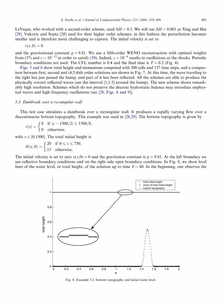
LeVeque, who worked with a second-order scheme, used DH = 0.1. We will use DH = 0.001 as Xing and Shu[29], Vukovic and Sopta [28] used for their higher order schemes: in this fashion the perturbation becomessmaller and is therefore more challenging to capture. The initial velocity is set to

vðx; 0Þ ¼ 0

and the gravitational constant g = 9.81. We use a fifth-order WENO reconstruction with optimal weightsfrom (37) and e = 10�12 in order to satisfy (39). Indeed, e = 10�6 results in oscillations at the shocks. Periodicboundary conditions are used. The CFL number is 0.4 and the final time is T = 0.2 (Fig. 4).

Figs. 5 and 6 show total height and momentum computed with 200 cells and 157 time steps, and a compar-ison between first, second and (4,5,4)th order solutions are shown in Fig. 7. At this time, the wave traveling tothe right has just passed the hump, and part of it has been reflected. All the schemes are able to produce thephysically correct reflected waves (see the interval [1,1.5] around the hump). The new scheme shows remark-ably high resolution. Schemes which do not preserve the discrete hydrostatic balance may introduce unphys-ical waves and high frequency oscillations (see [28, Figs. 8 and 9]).

3.3. Dambreak over a rectangular wall

This test case simulates a dambreak over a rectangular wall. It produces a rapidly varying flow over adiscontinuous bottom topography. This example was used in [28,29]. The bottom topography is given by

zðxÞ ¼8 if jx� 1500=2j 6 1500=8;

0 otherwise;

�

with x 2 [0,1500]. The total initial height is

Hðx; 0Þ ¼20 if 0 6 x 6 750;

15 otherwise.

�

The initial velocity is set to zero v(x,0) = 0 and the gravitation constant is g = 9.81. At the left boundary weuse reflective boundary conditions and on the right side open boundary conditions. In Fig. 8, we show levellines of the water level, or total height, of the solution up to time T = 60. In the beginning, one observes the

0 0.2 0.4 0.6 0.8 1 1.2 1.4 1.6 1.8 20

0.2

0.4

0.6

0.8

1

x

tota

l hei

ght

total initial heightzoom of total initial heightbottom topography

Fig. 4. Example 3.2, bottom topography and initial water level.

0 0.2 0.4 0.6 0.8 1 1.2 1.4 1.6 1.8 20.9999

1

1.0001

1.0002

1.0003

1.0004

1.0005

1.0006

x

tota

l hei

ght

200 cells T=0.2 (time step 157 )exact

Fig. 5. Example 3.2, total height at T = 0.2 computed with 200 cells.

0 0.2 0.4 0.6 0.8 1 1.2 1.4 1.6 1.8 2

0

0.5

1

1.5

2 x 10

x

mom

entu

m

200 cells T=0.2 (time step 157)exact

Fig. 6. Example 3.2, momentum at T = 0.2 computed with 200 cells.


standard rarefaction and shock waves which form the solution of the Riemann problem of the homogeneousshallow water equations. Figs. 9 and 10 show the water level and velocity at T = 15. At time T � 17 the wavescross the two edges of the wall. A part is transmitted, another part reflected, and a remaining part becomes astanding wave. Such standing waves have recently been studied analytically by Klausen and Risebro [17],Towers [27], Klingenberg and Risebro [18], and Seguin and Vovelle [21] who consider the inhomogeneous

0 0.2 0.4 0.6 0.8 1 1.2 1.4 1.6 1.8 20.9999

1

1.0001

1.0002

1.0003

1.0004

1.0005

1.0006

x

tota

l hei

ght

first, second, fifth order solution at T=0.2 (157 time steps) , with 200 cells

first order scheme

second order scheme

fourth order schemes

exact solution

Fig. 7. Example 3.2, total height at T = 0.2 computed with first, second, and (4,5,4)th order schemes and 200 cells.

0 500 1000 1500

100

200

300

400

500

600

700

800

x

times

tep

Fig. 8. Example 3.3, contour plot of water level in the x � t plane.


one dimensional shallow water equations as a system of three conservation laws for (h,hu,z) with ot z = 0. Thissystem has the three wave speeds u�

ffiffiffiffiffigh

pand 0. For later times, the wave system keeps interacting. At time

T = 60, we have six waves in the solution. The main shock and rarefaction waves just hit the boundary of thecomputational domain. Between them we have, from left to right, a standing wave, a weak rarefactiontraveling leftwards, a second standing wave, and a weak compressive wave traveling rightwards. Figs. 11and 12 show cross sections of total height and velocity. Note that the standing waves (which are contact

0 500 1000 15000

2

4

6

8

10

12

14

16

18

20

x

tota

l hei

ght

total height T=15 (time step 211)bottom topography

Fig. 9. Example 3.3, water level at T = 15,600 cells.

0 500 1000 1500

0

0.5

1

1.5

2

2.5

3

x

velo

city

velocity T=15 (time step 211)

Fig. 10. Example 3.3, velocity at T = 15,600 cells.


discontinuities) are not easy to capture. This is discussed, e.g., in [28]. Here we have almost perfect resolutionof all features of this challenging solution.

4. Two dimensional extension

The shallow water equations in 2D are given by

0 500 1000 15000

2

4

6

8

10

12

14

16

18

20

x

tota

l hei

ght

total height T=60 (time step 872)bottom topography

Fig. 11. Example 3.3, water level at T = 60,600 cells.

0 500 1000 15000

0.5

1

1.5

2

2.5

3

3.5

4

x

velo

city

velocity T=60 (time step 872)

Fig. 12. Example 3.3, velocity at T = 60,600 cells.


ht þ ðhuÞx þ ðhvÞy ¼ 0;

ðhuÞt þ hu2 þ 1

2gh2

� �x

þ ðhuvÞy ¼ �ghzx;

ðhvÞt þ ðhuvÞx þ hv2 þ 1

2gh2

� �y

¼ �ghzy ;

ð19Þ


where h is the water height, z is the bottom topography, u is the velocity in x-direction, v is the velocity iny-direction and g is the gravitational constant. We will now discuss how to extend our scheme to twodimensions.

4.1. Overview of the scheme

Rewrite the system (19) in the standard form:

Ut þ F xðUÞ þ GyðUÞ ¼ SðUÞ; ð20Þ
where clearly U = (h,hu,hv)T, F ¼ ðhu; hu2 þ 1
2gh2; huvÞT, G ¼ ðhv; huv; hv2 þ 1

2gh2ÞT and S = (0,�ghzx, �ghzy)

T.We define the cell averages over grid cells I ij ¼ ðxi�1

2; xiþ1

2Þ � ðyj�1

2; yjþ1

2Þ by

Uij ¼1

DxDy

ZIij

Uðx; yÞdxdy; ð21Þ

where Dx ¼ xiþ12� xi�1

2;Dy ¼ yjþ1

2� yj�1

2. Suppose for simplicity that the cells are square: let d = Dx = Dy. Inte-

grating each term in (19) over the cell Iij and invoking the divergence theorem, we get the following semidis-crete scheme for the evolution of the cell averages Uij:

d2d

dtU ijðtÞ þ

Z@Iij

ðF ;GÞ � nds ¼ZI ij

S dxdy;

Rewrite the system as:

d

dtUijðtÞ þ

F iþ12;j� F i�1

2;j

dþGi;jþ1

2� Gi;j�1

2

d¼ Sij; ð22Þ

where

F i�12;j¼ 1

d

Z yjþ12d

yj�12d

F ðUðxi�12; yÞÞdy; ð23Þ

Gi;j�12¼ 1

d

Z xiþ12d

xi�12d

GðUðx; yj�12ÞÞdx; ð24Þ

Sij ¼1

d2

ZI ij

Sðx; yÞdxdy. ð25Þ

In analogy with the 1D case, we reconstruct the variables h, hu, hv, and H, while the bottom topography isgiven by z = H � h. In general, this yields a discontinuous approximation of z. Let Uij(x,y) denote the recon-struction computed in the cell Iij with U denoting any of the reconstructed variables. Again, to preserve theequilibrium states, a hydrostatic reconstruction is needed on the quadrature points on the boundary of thecell, which will be denoted by h*:

h�iþ1;jðxþiþ12; �Þ ¼ max 0;Hiþ1;j xiþ1

2; �

�max zij xiþ1

2; �

; ziþ1;j xiþ1

2; �

;

h�ij x�iþ12; �

¼ max 0;Hij xiþ1

2; �

�max zij xiþ1

2; �

; ziþ1;j xiþ1

2; �

;

h�i;jþ1 �; yþjþ1

2

¼ max 0;Hi;jþ1 �; yjþ1

2

�max zij �; yjþ1

2

; zi;jþ1 �; xjþ1

2

;

h�ij �; y�jþ12

¼ max 0;Hij �; yjþ1

2

�max zij �; yjþ1

2

; zi;jþ1 �; yjþ1

2

.

To approximate the quantities F i�12;j

and Gi;j�12in (23) and (24), we use a quadrature

F i�12;j’Xk

xkF U xi�12; yj þ nkd

;


where xk and nk are the weights and nodes of the quadrature formula. For a fourth-order scheme we use theclassical two-point Gaussian formula

F i�12;j

’ 1

2F U xi�1

2; yj � ad

þ F U xi�1

2; yj þ ad

; ð26Þ

where a ¼ 1=ð2ffiffiffi3

pÞ. A similar formula holds for Gi;j�1

2.

We still need to construct a well balanced approximation to each of the flux evaluations required in (26). Asin 1D, the numerical flux is composed of two contributions. The first contribution (Fh for F and Gh for G) isconsistent with the flux of the homogeneous shallow water equations, the second contribution compensatesthe perturbation introduced by the hydrostatic correction.

The modified state variables that will be applied in the flux computations are

U �ij ¼

h�ijðhuÞijðhvÞij

0B@

1CA.

Along the edge ðxi�12; yÞ for instance the numerical fluxes are

FlðUi�1;j;Ui;j; zi�1;j; zi;jÞi�12;j�a

:¼ F hðU �i�1;j xi�1

2; yj � ad

;U �

ijðxi�12; yj � adÞÞ þ g

2

0

h2ij xi�12; yj � ad

� ðh�Þ2ij xi�1

2; yj � ad

0

0B@

1CA ð27Þ

and

FrðUi;j;Uiþ1;j; zi;j; ziþ1;jÞiþ12;j�a

:¼ F h U �i;j xiþ1

2; yj � ad

;U �

iþ1;j xiþ12; yj � ad

þ g

2

0

h2ij xiþ12; yj � ad

� ðh�Þ2ij xiþ1

2; yj � ad

0

0B@

1CA;

ð28Þ

with similar formulas for Gl and Gr.Thus the semidiscrete scheme can be written as,

d

dtU ijðtÞ ¼ � 1

2dFr

iþ12;jþa þFr

iþ12;j�a �Fl

i�12;jþa �Fl

i�12;j�a þ Gr

iþa;jþ12þ Gr

i�a;jþ12� Gl

iþa;j�12� Gl

i�a;j�12

þ Sij.

ð29Þ
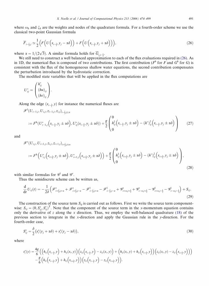
The construction of the source term Sij is carried out as follows. First we write the source term component-
wise: Sij ¼ ð0; Sxij; S

yijÞ

T. Note that the component of the source term in the x-momentum equation containsonly the derivative of z along the x direction. Thus, we employ the well-balanced quadrature (18) of theprevious section to integrate in the x-direction and apply the Gaussian rule in the y-direction. For thefourth-order case,

Sxij ¼

d2

sxi ðyj þ adÞ þ sxi ðyj � adÞ� �

; ð30Þ

where

sxi ðyÞ ¼4g6

hij xi�12; y

þ hijðxi; yÞ

zij xi�1

2; y

� zijðxi; yÞ

þ hijðxi; yÞ þ hij xiþ1

2; y

zijðxi; yÞ � zij xiþ1

2; y

� g

6hij xi�1

2; y

þ hij xiþ1

2; y

zij xi�1

2; y

� zij xiþ1

2; y

.


In the same fashion, we compute the source Syij using (18) in the y-direction and the Gaussian rule in the

x-direction. Again, in the fourth-order case:

Fig. 1recons(xi±a,y

Syij ¼

d2

syjðxi þ adÞ þ syjðxi � adÞ� �

; ð31Þ

where now,

syj ðxÞ ¼4g6

hij x; yj�12

þ hijðx; yjÞ

zij x; yj�1

2

� zijðx; yjÞ

þ hijðx; yjÞ þ hij x; yjþ1

2

zijðx; yjÞ � zij x; yjþ1

2

� g

6hij x; yj�1

2

þ hij x; yjþ1

2

zij x; yj�1

2

� zij x; yjþ1

2

.

Using the same arguments as in the proof of Theorem 3 one can show:

Corollary 5. The 2D scheme is fourth-order accurate and preserves the stationary state of the lake at rest.

4.2. 2D reconstruction

In order to evaluate the numerical flux functions F and G and the source term S, we need to reconstructpoint values of H, h, hu and hv at 12 integration points, 8 on the boundary ðxi�1

2; yj�aÞ; ðxi�a; yj�1

2Þ and 4 in the

interior (xi,yj±a) and (xi±a,yj) as shown on the right of Fig. 13. Note that the interior points are required onlyto compute the source term, which is fourth-order accurate. As in the 1D case we apply a WENO procedure tofind these data.

In 2D this reconstruction is somewhat more involved. Our approach is to reconstruct each variable dimen-sion by dimension. For each cell, the one dimensional WENO procedure has to be applied six times to producepoint values in all quadrature points.

To fix ideas, we illustrate the algorithm for the reconstruction of the variable h. In this section only, wedenote the cell averages as �hij, to distinguish the averages computed on a cell (a double integral) from the aver-ages computed along only one segment (a single integral).

We start applying the WENO reconstruction procedure in the y direction, starting from the cell averages�hij. We apply the reconstruction defined by the constants in Appendix A (38) and we find approximations inthe points (xi,yj+a) and (xi,yj�a) to the function:

�hijðxi; yj�aÞ ¼1

d

Z xiþd2

xi�d2

hðx; yj�aÞdx.

3. (Left) The positions of the reconstructed cross section averages (xi±a, Æ) (dashed lines), (Æ ,yj±a) (black lines) for the firsttruction step. (Right) The Gaussian integration points for the edges ðxi�1

2; yj�aÞ; ðxi�a; yj�1

2Þ and for the interior, (xi,yj±a) and

j). The point values in these locations are computed in the second step of the reconstruction.


Once these data are available for all i, we apply again the WENO reconstruction along the x axis to get therequired point values, i.e., hijðxi�1

2; yjþaÞ, hij(xi,yj+a) and hijðxiþ1

2; yjþaÞ, starting from �hijðxi; yjþaÞ. With another

reconstruction, we find hijðxi�12; yj�aÞ, hij(xi,yj�a) and hijðxiþ1

2; yj�aÞ, starting from �hijðxi; yj�aÞ. This set of oper-

ations will be called y–x sweep, see Fig. 14.To get the quadrature points along the dashed lines on the right in Fig. 13, we perform the same operations

in the reversed order. This will be called x-y sweep, see Fig. 15.Now, all the quantities appearing in the semidiscrete scheme (22) have been defined. Finally, to get a fully

discrete scheme, we need to specify a method to march forward in time. As in the 1D scheme, we apply theclassic fourth-order Runge–Kutta method. For other cases, it might be advantageous to use the recent TVD orSSP Runge–Kutta schemes [23,12,26].

4.3. Well-balanced test in two dimensions

The two dimensional experiments we present here follow closely the work of Xing and Shu [29]. We checkthe behavior of the two dimensional scheme in a lake at rest situation on a rectangular domain [0,1] · [0,1],with a non-flat, fully two-dimensional, bottom topography

Fig. 14side. Iðxi; yj�

Fig. 15side. In(right

zðx; yÞ ¼ 0:8e�50ððx�0:5Þ2þðy�0:5Þ2Þ. ð32Þ

. In the first step of the y–x-sweep we compute averages over cross sections (Æ ,yj±a) marked with black lines in the figure on the leftn the second step of the y–x-sweep we use the cross section averages to compute point values at quadrature points ðxi�1

2; yj�aÞ;

aÞ (right figure).

. In the first step of the x–y-sweep we compute averages over cross sections (Æ ,xi±a) marked with dotted lines in the figure on the leftthe second step of the x–y-sweep we use the cross section averages to compute point values at quadrature points ðxi�a; yj�1

2Þðxi�a; yjÞ

figure).


The initial water height is

TableL1-erro

Numb

2550100200400800

hðx; yÞ ¼ 1� zðx; yÞ; ð33Þ
so that the water surface level H is constant, with H ” 1.0. The momentum in x and y direction is set to zero:
huðx; y; t ¼ 0Þ ¼ 0 and hvðx; y; t ¼ 0Þ ¼ 0. ð34Þ
The lake is at rest initially, and should remain at rest indefinitely. In this situation, a scheme without well-balancing would produce unphysical waves. For this test we use a uniform 100 · 100 grid and compute thesolution at time t = 0.1. We get the following L1-errors for the conservative components: ihi1 = 1.23E�16,ihui1 = 2.20E�16 and ihvi1 = 2.22E�16. The errors are all of the magnitude of the rounding error 10�16 thusthe scheme is indeed perfectly well-balanced.
4.4. Testing the order of accuracy

To check the numerical order of accuracy we use the same experiment as Xing and Shu [29]. On the unitsquare [0,1] · [0,1] we choose the bottom topography:

zðx; yÞ ¼ sinð2pxÞ þ cosð2pyÞ
the initial water surface level:
hðx; y; t ¼ 0Þ ¼ 10þ esinð2pxÞ cosð2pyÞ
and the initial momentum in the x and y directions, respectively:
huðx; y; t ¼ 0Þ ¼ sinðcosð2pxÞÞ sinð2pyÞ;hvðx; y; t ¼ 0Þ ¼ cosð2pxÞ cosðsinð2pyÞÞ.

We compute up to time T = 0.05 with CFL-number 0.8. For the WENO reconstruction we use the optimalweights of 37,38 and set e = 10�6. The reference solution is computed with the same scheme and 1600 ·1600 cells, since the exact solution is unknown.

For this experiment we expect fourth-order of accuracy in all conservative components. The applied stan-dard Runge–Kutta time integration, the integration of the numerical fluxes with Gaussian rule and the cellcentered source term are all formally fourth-order accurate, while the applied WENO reconstruction isfifth-order accurate. Table 3 contains the L1-errors and orders of accuracy. We can clearly see that for thistwo dimensional test case, fourth-order accuracy (in fact almost fifth-order) is indeed achieved in allcomponents.

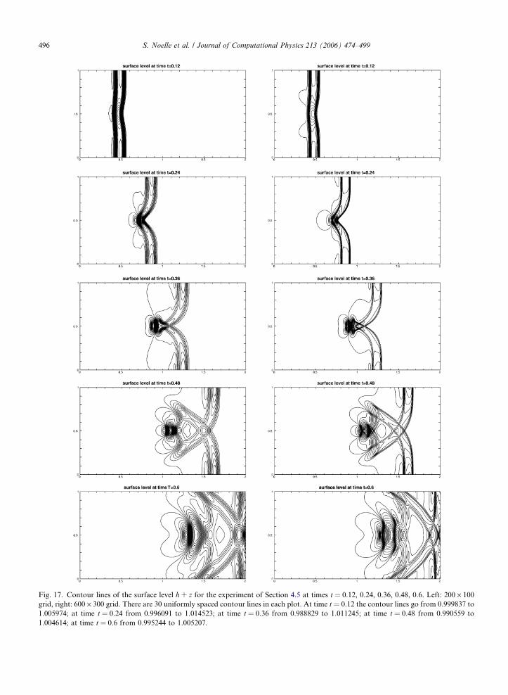
4.5. A small perturbation of a two dimensional steady-state lake

This classical problem is given by LeVeque [20] and is also computed in [29]. For this problem we considerthe rectangular domain [0,2] · [0,1]. The bottom topography is displayed in Fig. 16 and it is given by:

zðx; yÞ ¼ 0:8e �5ðx�0:9Þ2�50ðy�0:5Þ2ð Þ.

3rs and numerical order of accuracy for the convergence test 4.4

er of points CFL h hu hv

L1 error Order L1 error Order L1 error Order

0.5 8.77E � 03 3.42E � 02 6.71E � 020.5 1.10E � 03 3.00 2.73E � 03 3.65 9.40E � 03 2.840.5 9.84E � 05 3.48 1.56E � 04 4.13 7.85E � 04 3.580.5 4.91E � 06 4.32 6.58E � 06 4.57 3.93E � 05 4.320.5 1.82E � 07 4.76 2.41E � 07 4.77 1.46E � 06 4.750.5 6.06E � 09 4.91 7.94E � 09 4.92 4.90E � 08 4.90

0

0.5

1

1.5

2

0

0.5

10

0.2

0.4

0.6

0.8

xy

Fig. 16. Bottom topography of experiment 4.5 zðx; yÞ ¼ 0:8eð�5ðx�0:9Þ2�50ðy�0:5Þ2Þ.


The initial water surface level is given by:

hðx; y; t ¼ 0Þ ¼1:01� zðx; yÞ if 0:05 6 x 6 0:15;

1� zðx; yÞ otherwise;

�

so the initial surface level is almost flat, only in the region 0.05 < x < 0.15 it is perturbed upward by the dis-placement 0.01. The initial momentum in the x and y directions is:

huðx; y; t ¼ 0Þ ¼ 0;

hvðx; y; t ¼ 0Þ ¼ 0.

We compute using two different uniform meshes with 200 · 100 cells and 600 · 300 cells.Fig. 17 shows 30 uniformly spaced contour lines of the surface level H at times t = 0.12,0.24,0.36,0.48 and

final time T = 0.6. The results obtained with the coarse grid appear on the left side, while on the right we findthe numerical solution obtained with the fine grid.

In the simulation with the coarse grid we use e = 10�6 and for the fine grid e = 10�9. In both experiments wechoose the CFL-number equal to 0.5. As we can see, we get results comparable to the finite differenceapproach in [29].

5. Conclusion

In this paper, we have constructed well-balanced finite volume schemes for the shallow water equations,which are of any desired order of accuracy. The new schemes generalize a class of second-order schemes pro-posed by Audusse et al. [1]. A (4,5,4)th order version of the new scheme gives the expected high resolutionboth for smooth and non-smooth flows, and perfect balance for the lake at rest in one and two spatial direc-tions. The key technique, a new quadrature formula for the source term, can be applied to a wide variety offirst and second-order well balanced schemes, to raise their order of accuracy. Work on stable schemes forflows with dry areas is in progress.

We would like to thank an unknown referee for pointing us to the recent preprints [30,31], where a class ofmore general balance laws is treated via different techniques. Our high order accurate quadrature technique

Fig. 17. Contour lines of the surface level h + z for the experiment of Section 4.5 at times t = 0.12, 0.24, 0.36, 0.48, 0.6. Left: 200 · 100grid, right: 600 · 300 grid. There are 30 uniformly spaced contour lines in each plot. At time t = 0.12 the contour lines go from 0.999837 to1.005974; at time t = 0.24 from 0.996091 to 1.014523; at time t = 0.36 from 0.988829 to 1.011245; at time t = 0.48 from 0.990559 to1.004614; at time t = 0.6 from 0.995244 to 1.005207.



using extrapolation carries over to that class as well, and it will be well-balanced exactly if the continuity con-dition (4.8) of [31] holds. For the lake at rest, (4.8) is given by the hydrostatic reconstruction, but for eachsystem of balance laws, an analogous technique has to be established (seperately for each scheme). We willleave this to future work.

Acknowledgements

We are grateful to two unknown referees for asking inspiring questions about the deeper mechanism of ourbalancing approach. Moreover, we would like to thank Francois Bouchut for lively and stimulating discus-sions. Francois gave us a version of his first and second-order well-balanced scheme. We would also like tothank the Institute of Hydraulic Engineering and Water Resources Management of RWTH Aachen for pro-viding the topographical data of lake Rursee. Part of this work was done while the first author was in residenceat CMA, ‘‘Center of Mathematics for Application’’ at Oslo University. The first and second authors wouldlike to thank CMA and its members for their generous hospitality.

Appendix A. WENO reconstruction

For completeness, we review the WENO reconstruction [15,24] for uniform grids in 1D. We aim to givesufficient details of all parameters so that the reader could reconstruct our algorithm and recover the numer-ical experiments. Necessarily, we present this as concisely as possible. For more details, we refer to the relevantliterature.

A main ingredient that we were not able to find elsewhere in the literature are the accuracy constants for thepoints in the Gaussian quadrature at the edges of the two-dimensional cells.

Given cell averages

ui :¼1

jCij

ZCi

uðxÞdx

on cell Ci of a smooth function u(x) and a fixed point x* 2 Cj, the WENO procedure provides a highly accu-rate piecewise polynomial approximation R(x*) of u(x*).

Rðx�Þ ¼ uðx�Þ þ OðDx2r�1Þ ð35Þ

1. Define r small stencils, composed of r cells, around the cell containing xj

Sk :¼ ðxjþk�rþ1; xjþk�rþ2; . . . ; xjþkÞ; k ¼ 0; . . . ; r � 1

and one large stencil

T :¼[r�1

k¼0

Sk

which contains all the cells from the r smaller stencils.2. Given cell averages uj compute the interpolation polynomials pk(x) of degree (r � 1) associated with the

stencils Sk for k = 0, . . ., r � 1 and the higher order reconstruction polynomial Q(x), of degree (2r�1) asso-ciated with the large stencil T. Here, interpolation is understood in the sense of cell averages.

3. Find the linear weights Cr0; . . . ;C

rr�1 such that:

Qðx�Þ ¼Xr�1

k¼0

Crkpkðx�Þ. ð36Þ

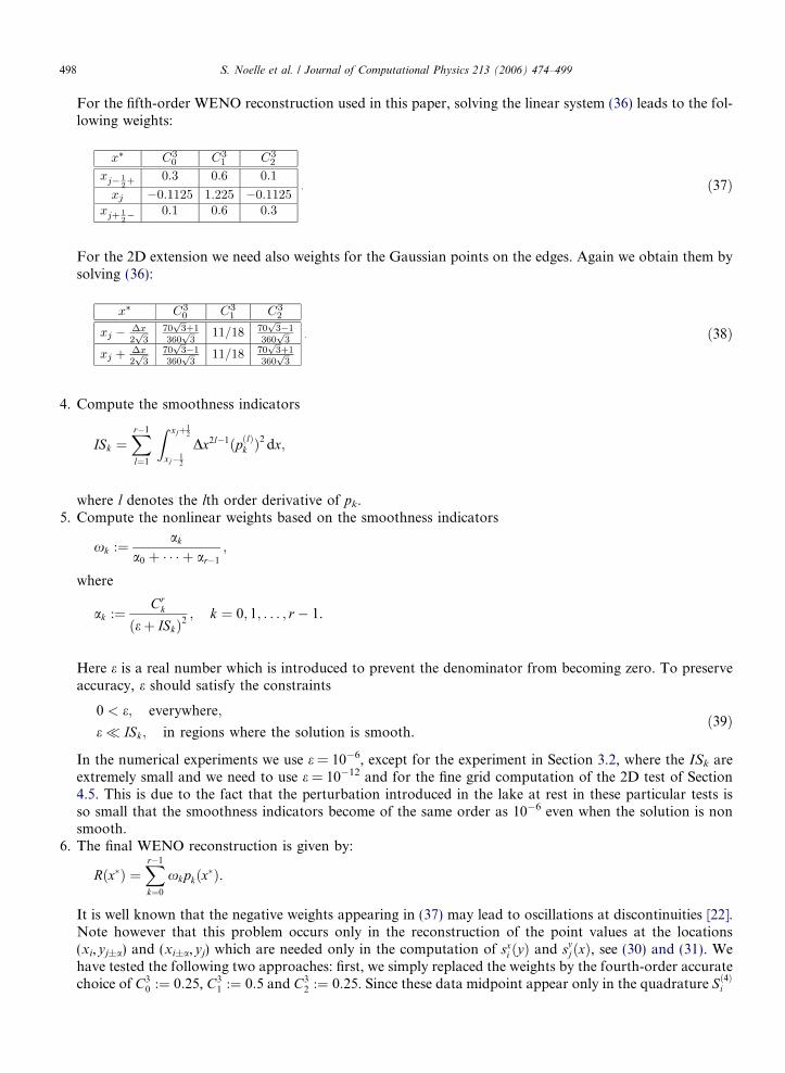
For the fifth-order WENO reconstruction used in this paper, solving the linear system (36) leads to the fol-lowing weights:


ð37Þ

For the 2D extension we need also weights for the Gaussian points on the edges. Again we obtain them bysolving (36):

ð38Þ

4. Compute the smoothness indicators

ISk ¼Xr�1

l¼1

Z xjþ12

xj�12

Dx2l�1ðpðlÞk Þ2 dx;

where l denotes the lth order derivative of pk.5. Compute the nonlinear weights based on the smoothness indicators

xk :¼ak

a0 þ � � � þ ar�1

;

where

ak :¼Cr

k

ðeþ ISkÞ2; k ¼ 0; 1; . . . ; r � 1.

Here e is a real number which is introduced to prevent the denominator from becoming zero. To preserveaccuracy, e should satisfy the constraints

0 < e; everywhere;

e � ISk; in regions where the solution is smooth.ð39Þ

In the numerical experiments we use e = 10�6, except for the experiment in Section 3.2, where the ISk areextremely small and we need to use e = 10�12 and for the fine grid computation of the 2D test of Section4.5. This is due to the fact that the perturbation introduced in the lake at rest in these particular tests isso small that the smoothness indicators become of the same order as 10�6 even when the solution is nonsmooth.

6. The final WENO reconstruction is given by:

Rðx�Þ ¼Xr�1

k¼0

xkpkðx�Þ.

It is well known that the negative weights appearing in (37) may lead to oscillations at discontinuities [22].Note however that this problem occurs only in the reconstruction of the point values at the locations(xi,yj±a) and (xi±a,yj) which are needed only in the computation of sxi ðyÞ and syjðxÞ, see (30) and (31). Wehave tested the following two approaches: first, we simply replaced the weights by the fourth-order accuratechoice of C3

0 :¼ 0:25, C31 :¼ 0:5 and C3

2 :¼ 0:25. Since these data midpoint appear only in the quadrature Sð4Þi


for the source term, which is only fourth-order accurate anyway, this does not decrease the overall order(4,5,4) of the algorithm. The second cure is the splitting technique of Shi, Hu and Shu [22]. For the prob-lems presented in this paper, this more expensive approach did not lead to superior results.

References

[1] E. Audusse, F. Bouchut, M.-O. Bristeau, R. Klein, B. Perthame, A fast and stable well-balanced scheme with hydrostaticreconstruction for shallow water flows, SIAM J. Sci. Comp. 25 (2004) 2050–2065.

[2] D.S. Bale, R.J. LeVeque, S. Mitran, J.A. Rossmanith, A wave propagation method for conservation laws and balance laws withspatially varying flux functions, SIAM J. Sci. Comp. 24 (2002) 955–978.

[3] A. Bermudez, M.E. Vazquez, Upwind methods for hyperbolic conservation laws with source terms, Comput. Fluids 23 (1994) 1049–1971.

[4] N. Botta, R. Klein, S. Langenberg, S. Lutzenkirchen, Well-balanced finite volume methods for nearly hydrostatic flows, J. Comp.Phys. 196 (2004) 539–565.

[5] F. Bouchut, J. Le Sommer, V. Zeitlin, Frontal geostrophic adjustment and nonlinear-wave phenomena in one dimensional rotatingshallow water. Part 2: high-resolution numerical simulations, J. Fluid Mech. 514 (2004) 35–63.

[6] F. Bouchut, M. Westdickenberg, Gravity driven shallow water models for arbitrary topography, Comm. Math. Sci. 2 (2004) 359–389.[7] P. Deuflhard, F. Bornemann, Numerische Mathematik 2., Anfangs- und Randwertprobleme gewohnlicher Differentialgleichungen, de

Gruyter, (2002), ISBN 3-11-017181-3.[8] T. Gallouet, J. Herard, N. Seguin, Some approximate Godunov schemes to compute shallow-water equations with topography,

Comput. Fluids 32 (2003) 479–513.[9] B. Gjevik, H. Moe, A. Ommundsen, Idealized model simulations of barotropic flow on the Catalan shelf, Continental Shelf Res. 22

(2002) 173–198.[10] L. Gosse, A.-Y. LeRoux, A well-balanced scheme designed for inhomogeneous scalar conservation laws, C.R. Acad. Sci. Paris Ser. I

Math. 323 (1996) 543–546.[11] L. Gosse, A well-balanced flux-vector splitting scheme designed for hyperbolic systems of conservation laws with source terms, Comp.

Math. Appl. 39 (2000) 135–159.[12] S. Gottlieb, C.-W. Shu, E. Tadmor, Strong stability-preserving high-order time discretization methods, SIAM Rev. 43 (2001) 89–112.[13] J.M. Greenberg, A.Y. LeRoux, A well-balanced scheme for the numerical processing of source terms in hyperbolic equations, SIAM

J. Num. Anal. 33 (1996) 1–16.[14] R. Holdahl, H. Holden, K.-A. Lie, Unconditionally stable splitting methods for the shallow water equations, BIT 39 (1999) 451–472.[15] G. Jiang, C.-W. Shu, Efficient implementation of weighted ENO schemes, J. Comp. Phys. 126 (1996) 202–228.[16] S. Jin, A steady-state capturing method for hyperbolic systems with geometrical source terms, M2ANMath. Model. Numer. Anal. 35

(2001) 631–645.[17] R.A. Klausen, N.H. Risebro, Stability of conservation laws with discontinuous coefficients, J. Diff. Eqn. 157 (1999) 41–60.[18] C. Klingenberg, N.H. Risebro, Stability of a resonant system of conservation laws modeling polymer flow with gravitation, J. Diff.

Eqn. 170 (2001) 344–380.[19] A. Kurganov, D. Levy, Central-upwind schemes for the Saint-Venant system, M2ANMath. Model. Numer. Anal. 36 (2002) 397–425.[20] R.J. LeVeque, Balancing source terms and flux gradients in high-resolution Godunov methods: the quasi-steady wave-propagation

algorithm, J. Comp. Phys. 146 (1998) 346–356.[21] N. Seguin, J. Vovelle, Analysis and approximation of a scalar conservation law with a flux function with discontinuous coefficient,

M3AS 13 (2003) 221–257.[22] J. Shi, C. Hu, C.-W. Shu, A technique of treating negative weights in WENO schemes, J. Comp. Phys. 175 (2002) 108–127.[23] C.-W. Shu, Total-variation-diminishing time discretization, SIAM J. Sci. Statist. Comp. 9 (1988) 1073–1084.[24] C.-W. Shu, Essentially non-oscillatory and weighted essentially non-oscillatory schemes for hyperbolic conservation laws, in: B.

Cockburn, C. Johnson, C.W. Shu, E. Tadmor (Eds.), Advanced Numerical Approximation of Nonlinear Hyperbolic Equations,Lecture Notes in Mathematics, Springer-Verlag, Berlin/New York, 1998, pp. 325–432.

[25] C.-W. Shu, S. Osher, Efficient implementation of essentially non-oscillatory shock capturing schemes, J. Comp. Phys. 77 (1988) 439.[26] R.J. Spiteri, S.J. Ruuth, A new class of optimal high-order strong-stability-preserving time discretization methods, SIAM J. Num.

Anal. 40 (2) (2002) 469–491.[27] J.D. Towers, Convergence of a difference scheme for conservation laws with a discontinuous flux, SIAM J. Num. Anal. 38 (2000) 681–

698.[28] S. Vukovic, L. Sopta, ENO and WENO schemes with the exact conservation property for one-dimensional shallow water equations,

J. Comp. Phys. 179 (2002) 593–621.[29] Y. Xing, C.-W. Shu, High order finite difference WENO schemes with the exact conservation property for the shallow water

equations, J. Comp. Phys. 208 (2005) 206–227.[30] Y. Xing C.-W. Shu, High order well-balanced finite difference WENO schemes for a class of hyperbolic systems with source terms, J.

Sci. Comp. (to appear).[31] Y. Xing, C.-W. Shu, High order well-balanced finite volume WENO schemes and discontinuous Galerkin methods for a class of

hyperbolic systems with source terms, J. Comp. Phys. Brown Scientific Computing Report BrownSC-2005-08, Available from:<http://www.dam.brown.edu/scicomp/publications/publications.htm> (submitted for publication).

http://www.dam.brown.edu/scicomp/publications/publications.htm

Date post:	11-Mar-2018
Category:	Documents
Upload:	vodung
View:	215 times
Download:	0 times

of accuracy for shallow water ﬂows q - News | IGPM accuracy for shallow water ﬂows q Sebastian...

Documents