~OF~ - DTIC

~OF~

Isolated Digit Recognition

Without Time Alignment

THESISJeffrey Mark GayCaptain, USAF

AFIT/GE/ENG/94D- 12

DEPARTMENT OF THE AIR FORCE

AIR UNIVERSITY

AIR FORCE INSTITUTE OF TECHNOLOGY

Wright-Patterson Air Force Base, Ohio

AFIT/GE/ENG/94D- 12



THESISJeffrey Mark Gay

Captain, USAF

AFIT/GE/ENG/94D- 12

Approved for public release; distribution unlimited

Acknowledgements

As is the case with any worthwhile work, this thesis was a team effort. There are many

key players that I would like to thank. First, I thank my Father in Heaven for blessing me with

the abilities that I have and for guiding me through this stressful period here at AFIT. It is to

His glory that this work is dedicated. Next, I thank my wife, JoNell. Without your wonderful

and loving support I could not have made it through this program. You encouraged me, fed

me, and never complained about the long hours and what must have been a lonely eighteen

months. I love you JoNell, and I thank God daily for bringing you into my life. I also owe a

great deal to my advisor, Dr Martin DeSimio. Thanks for the encouragement and for taking

me on as your charge in this effort. Without your help and expertise, this thesis would never

have been completed. Also, many thanks to the guys in the study team. We accomplished

things that would have been impossible alone. I am indebted to you all for helping me through

the tough course work leading up to this thesis. I owe a special note of thanks to Captain

Dave Jennings. The ideas that came from a conversation that we had resulted in a major

breakthrough in this work. Finally, to Terry and Shelley. Thanks for keeping the faith with

JoNell and me through this difficult period in our lives. We made it through with our dreams

intact and we're pressing on to Diamond. Ain't it great! See you at the top!

Jeffrey Mark Gay

/!,..ce::ojm For

CiTiSa C. I

\j --j7I I'...

"ii

AFIT/GE/ENG/94D- 12



THESIS

Presented to the Faculty of the School of Engineering

of the Air Force Institute of Technology

Air University

In Partial Fulfillment of the

Requirements for the Degree of

Master of Science in Electrical Engineering

Jeffrey Mark Gay, BSEE

Captain, USAF

Dec, 1994

Approved for public release; distribution unlimited

Table of Contents

Page

Acknowledgements ............................... ii

List of Figures .......... ................................. vii

List of Tables .......... .................................. viii

Abstract ............ .................................... xiii

I. Introduction ......... ............................... 1-1

1.1 Background ........ ......................... 1-1

1.2 Problem Description ........ .................... 1-2

1.3 Assumptions ......... ........................ 1-2

1.4 Scope ......... ............................ 1-3

1.5 Approach and Methodology ...... ................. 1-3

1.6 Materials and Equipment ......................... 1-4

1.7 Conclusions ........ ......................... 1-4

II. Literature Review ......... ............................ 2-1

2.1 Introduction ........ ......................... 2-1

2.2 Dynamic Time Warping and Hidden Markov Models . . .. 2-1

2.3 Artificial Neural Networks ...... ................. 2-2

2.4 Real-Time Recognition of Spoken Words ............... 2-4

2.5 Digit Recognition Using Vector Quantization ............. 2-4

2.6 Digit Recognition Using Neural Networks ............... 2-5

2.7 Conclusions ........ ......................... 2-6

ii

Page

III. Methodology .......... .............................. 3-1

3.1 Introduction ........ ......................... 3-1

3.2 Feature Extraction, ESPS ....... .................. 3-1

3.2.1 Conversion to ESPS Format ................. 3-2

3.2.2 Converting Sampled Data to Acoustic Features . . 3-3

3.3 Time/Frequency Averaged Spectrograms ..... .......... 3-5

3.3.1 Critical Band Energy Features ................ 3-5

3.3.2 Energy Profile Feature Extraction .............. 3-8

3.4 DTW with Critical Band Energy Features ............... 3-9

3.5 Concatenation of Feature Vectors ...... .............. 3-9

3.5.1 Averaged LPC and LPC Cepstral Features ..... 3-9

3.6 Baseline Experiments/Dynamic Time Warping ........... 3-10

3.6.1 List Preparation ....... .................. 3-10

3.7 Recognition Without Time Alignment ................. 3-12

3.7.1 Experiments Using LNKnet ................. 3-12

3.8 Quantifying the Results ....... ................... 3-15

3.9 Summary ........ .......................... 3-15

IV. Results .......... ................................. 4-1

4.1 Introduction ........ ......................... 4-1

4.2 Optimum Feature Length Determination ................ 4-2

4.3 Dynamic Time Warping .......................... 4-4

4.3.1 DTW Results Using LPC Cepstral Features . . . 4-4

4.4 DTW Results Using Critical Band Energy Features ..... 4-5

4.5 Results For Recognition Without Time Alignment ...... .... 4-10

4.5.1 Critical Band Energy Feature Classification . . . . 4-10

4.5.2 Results Using Concatenated Feature Vectors . . . . 4-10

iii

Page

4.5.3 Critical Band Energy, Averaged LPC Cepstral, and

LPC Features ....... ................... 4-13

4.6 Accuracy Comparison for Various Feature Sets ........... 4-16

4.7 Statistical Hypothesis Testing ...................... 4-18

4.8 Performance Breakdown ....... .................. 4-20

4.9 Conclusions ........ ......................... 4-23

V. Conclusions and Recommendations ....... ................... 5-1

5.1 Conclusions ........ ......................... 5-1

5.2 Accomplishments ........ ...................... 5-1

5.3 Recommendations ........ ..................... 5-2

5.3.1 Expanding the Vocabulary .................. 5-2

5.3.2 Performance in Noise ...... ............... 5-2

5.3.3 How Does It Work? . . . . . .. . . . . . . . . . .. . . . . . 5-3

5.3.4 Real-time Recognizer ...... ............... 5-3

Appendix A. Experimental Results ....... .................... A-1

A.1 Introduction ........ ......................... A-1

A.2 Classifier Accuracy Comparison ...... .............. A-1

A.3 Results For Individual Feature Sets .................. A-1

A.3.1 Critical Band Energy Feature Set ..... ......... A-3

A.3.2 Energy Profile Feature Set .................. A-11

A.3.3 LPC Cepstral Coefficient Feature Set .... ....... A-13

A.3.4 LPC Coefficient Feature Set ................. A-16

A.4 Experiments With Concatenated Vectors ..... .......... A-19

A.4.1 Critical Band Energy and Energy Profile Features A-19

A.4.2 Critical Band Energy and LPC Coefficient Features A-21

A.4.3 Critical Band Energy and LPC Cepstral Features . A-24

iv

Page

A.4.4 Critical Band Energy, LPC Cepstral, and LPC Coeffi-

cient Features ...... ................... A-27

Appendix B. C-shells ......... .......................... B-1

B.l Introduction ........ ......................... B-1

B.2 C-shells for Controlling ESPS Experiments .............. B-1

B.2.1 Binary to Sampled Data Conversion ............ B-2

B.2.2 Segmenting Sampled Data Files ............... B-2

B.2.3 Converting Sampled Data Files to Acoustic Feature

Files ........ ........................ B-2

B.2.4 Generic Header Item ...... ............... B-5

B.2.5 Performing Dynamic Time Warping ............ B-6

B.2.6 Quantifying The Results From ESPS ............ B-8

B.2.7 Converting MATLAB Files to ESPSFEA Files . . . B-12

B.3 C-shells For Controlling LNKnet Experiments .... ....... B-12

B.3.1 Preparing The Data For LNKnet .............. B-12

B.3.2 Setting The Defaults ...................... B-13

B.3.3 Classifying The Features With LNKnet .......... B-15

B.3.4 Quantifying The Results ................... B-16

B.3.5 Obtaining an Overall Confusion Matrix .......... B-18

B.4 Feature Vector Averaging ....... .................. B-27

Appendix C. MATLAB Files ........ ........................ C-1

C.1 Introduction ........ ......................... C-1

C.2 Critical Band Energy Feature Calculation for the Training Data

Set ......... ............................. C-1

C.3 Critical Band Energy Feature Calculation for the Testing Data

Set ......... ............................. C-4

C.4 Adding The Class Indicator To The Feature Vectors ..... C-7

v

Page

C.5 Energy Window Computation ................ C-10

C.6 Concatenating Feature Vectors ...... ............... C-12

C.6.1 Removing The Classes From A Feature Set . . .. C-13

C.7 Statistical Hypothesis Testing ...................... C-14

Bibliography .......... .................................. BIB-1

Vita .......... ...................................... VITA-1

vi

List of Figures

Figure Page

2.1. A multi-layer perceptron with one hidden layer .................. 2-3

3.1. Example digit "six," illustrating silence surrounding each utterance. . . 3-2

3.2. Pre-emphasis filter magnitude response ....................... 3-4

3.3. Spectrogram of the digit "zero." ....... ................... 3-6

3.4. The mel scale ......... .............................. 3-6

3.5. Typical 9-element critical band energy feature vectors for ten utterances of

the digit zero by speaker ml .............................. 3-7

3.6. Segmentation by envelope detection: (a) Original utterance of the digit"six," (b) Absolute value of the utterance, (c) Envelope of the utterance

(with threshold), (d) Segmented utterance ...................... 3-8

3.7. Typical averaged 12th-order LPC cepstral features for ten utterances of the

digit "zero." . ....... ............................. 3-11

3.8. Typical averaged 1 0th-order LPC coefficient features for ten utterances of

the digit "zero.. . ................................. 3-11

3.9. Typical processing steps for classification using DTW with the LPC cepstral

feature set ........... .............................. 3-12

3.10. Typical processing steps for classification using a MLP with the critical

band energy feature set ........ ......................... 3-13

3.11. A MLP classifier that considers three different sets of features ...... ... 3-14

4.1. Comparison of recognition accuracy versus the number of elements per

feature vector using both male and female speakers ................ 4-2


feature vector using male speakers only. ...................... 4-3


feature vector using female speakers only ...................... 4-3

vii

List of Tables

Table Page

4.1. Confusion matrix for DTW classification using LPC cepstral features with

both male and female speakers ....... ..................... 4-5

4.2. Overall results for DTW classification using LPC cepstral features with

both male and female speaker sets ........................... 4-6

4.3. Confusion matrix for DTW classification using critical band energy features

and a short reference list with both male and female speaker sets .... 4-7

4.4. Overall results for DTW classification using critical band energy features

and a short reference list with both male and female speaker sets ..... 4-7


and a short reference list with male speakers only ................. 4-8


and a short reference list with male speakers only ................. 4-8


and a long reference list with male speakers only ................. 4-9


and a long reference list with male speakers only ................. 4-9

4.9. Confusion matrix for the MLP classifier using critical band energy features

for both the male and female speakers with nine-element feature vectors. 4-11

4.10. Overall results for the MLP classifier with critical band energy features for

both the male and female speakers using 9-element feature vectors. . . 4-11

4.11. Confusion matrix for the MLP classifier with critical band energy features

for male speakers only using 9-element feature vectors ............. 4-12

4.12. Overall results for the MLP classifier with critical band energy features for

male speakers only using 9-element feature vectors ............... 4-12

4.13. Confusion matrix for MLP classification using concatenated critical band

energy and averaged 10th-order LPC coefficient features for male speakers

only ......... ................................... 4-14

viii

Table Page

4.14. Overall results for MLP classification using concatenated critical band

energy and averaged 10th-order LPC coefficient features for male speakers

only ........... ................................. 4-14


energy and averaged 12th-order LPC cepstrum features for male speakers

only ........... ................................. 4-15


energy and averaged 12th-order LPC cepstrum features for male speakers

only. ......... .................................. 4-15


energy, averaged LPC cepstrum, and averaged LPC coefficient features for

male speakers only. ................................. 4-16


energy, averaged LPC cepstrum, and averaged LPC coefficient features for

male speakers only ........ ........................... 4-17

4.19. Comparison of MLP recognition accuracy for the original critical band

energy features and the various concatenated feature sets ............ 4-17

4.20. Per speaker recognition accuracies for male speakers only. The confidenceinterval for the overall results is 95% ....... .................. 4-19

4.21. Per speaker recognition accuracies for both male and female speaker sets.

The confidence interval for the overall results is 95% .............. 4-19

4.22. Error synopsis for male-only speaker-independent recognition using con-

catenated critical band energy, LPC cepstral, and LPC coefficient features. 4-21

4.23. Error synopsis for male-only speaker-independent recognition using the

critical band energy features .............................. 4-21


LPC cepstral features ........ .......................... 4-22


LPC coefficient features ................................ 4-22

A. 1. MLP classifier accuracy per number of features for male, female, and

complete speaker sets using critical band energy features ........ .... A-2

ix

Table Page

A.2. KNN classifier accuracy per number of features for male, female, and


A.3. Gaussian classifier accuracy per number of features for male, female, and


A.4. Confusion matrix for the MLP classifier using critical band energy features

for the female speaker set ................................ A-3

A.5. Overall results for the MLP classifier using critical band energy features


A.6. Confusion matrix for the KNN classifier using critical band energy features

for both the male and female speakers using 9-element feature vectors.. A-4

A.7. Overall results for the KNN classifier using critical band energy features

for both the male and female speakers using 9-element feature vectors.. A-5

A.8. Confusion matrix for the KNN classifier using critical band energy features

for the male speaker set ................................. A-5

A.9. Overall results for the KNN classifier using critical band energy features


A. 10. Confusion matrix for the KNN classifier using critical band energy features


A. 11. Overall results for the KNN classifier using critical band energy features


A.12. Confusion matrix for the Gaussian classifier using critical band energy

features for both the male and female speakers using 9-element feature

vectors ......... ................................. A-7

A. 13. Overall results for the Gaussian classifier using critical band energy features

for both the male and female speakers with 9-element feature vectors. A-8

A. 14. Confusion matrix for the Gaussian classifier using critical band energy

features for the male speaker set ........................... A-8



A.16. Confusion matrix for the Gaussian classifier using critical band energy

features for the female speaker set ........................... A-9

x

Table Page


for the female speaker set ............................... A-10

A. 18. Confusion matrix results for the MLP classifier using energy profile features

for the male speaker set ................................ A-11

A. 19. Overall results for the MLP classifier using energy profile features for the

male speaker set ........... .......................... A- 12

A.20. Confusion matrix for the MLP classifier using 12th-order LPC cepstralfeatures for both the male and female speaker sets ................. A-13

A.21. Overall results for the MLP classifier using 12th-order LPC cepstral fea-

tures for both the male and female speaker sets .................. A-14

A.22. Confusion matrix for the MLP classifier using 12th-order LPC cepstral

features for the female speaker set .......................... A-14

A.23. Overall results for the MLP classifier using 12th-order LPC cepstral fea-

tures for the female speaker set ........................... A-15

A.24. Confusion matrix for the MLP classifier using 10th-order LPC coefficient

features for both the male and female speaker sets ................. A-16

A.25. Overall results for the MLP classifier using 10th-order LPC coefficient

features for both the male and female speaker sets ................. A-17

A.26. Confusion matrix for the MLP classifier using 1Oth-order LPC coefficient


A.27. Overall results for the MLP classifier using 10th-order LPC coefficient


A.28. Confusion matrix for the MLP classifier using concatenated critical band

and energy profile features for male speakers only. .... ........... A-19

A.29. Overall results for the MLP classifier using concatenated critical band and

energy profile features for male speakers only.. ................. A-20

A.30. Confusion matrix for the MLP classifier using concatenated critical band

energy and averaged 10th-order LPC coefficient features for female speak-

ers only. ......... ................................ A-21

A.3 1. Overall results for the MLP classifier using concatenated critical band en-

ergy and averaged 10th-order LPC coefficient features for female speakers

only. ......... .................................. A-22

xi

Table Page

A.32. Confusion matrix for the MLP classifier using concatenated critical bandenergy and averaged 10th-order LPC coefficient features for both male and

female speakers ............................. A-22

A.33. Overall results for the MLP classifier using concatenated critical bandenergy and averaged 10th-order LPC coefficient features for both male and


A.34. Confusion matrix for the MLP classifier using concatenated critical bandenergy and averaged 12th-order LPC cepstral features for female speakers

only. . . . . . . . . . . . . . . . . . . . . . . . . . . . . . . . . . . A -24

A.35. Overall results for the MLP classifier using concatenated critical bandenergy and averaged 12th-order LPC cepstral features for female speakers

onl y .. . . . . . . . . . . . . . . . . . . . . . . . . . . . . . . . . . A -25

A.36. Confusion matrix for the MLP classifier using concatenated critical bandenergy and averaged 12th-order LPC cepstral features for both male and


A.37. Overall results for the MLP classifier using concatenated critical bandenergy and averaged 12th-order LPC cepstral features for both male and


A.38. Confusion matrix for the MLP classifier using concatenated critical bandenergy, averaged 12th-order LPC cepstrum, and averaged 10th-order LPC

coefficient features for female speakers only. .............. A-27

A.39. Overall results for the MLP classifier using concatenated critical bandenergy, averaged 12th-order LPC cepstral, and averaged 10th-order LPC

coefficient features for female speakers only ............... A-28

A.40. Confusion matrix for the MLP classifier using concatenated critical bandenergy, averaged 12th-order LPC cepstral, and averaged 10th-order LPC

coefficient features for both male and female speakers .......... A-28

A.41. Overall results for the MLP classifier using concatenated critical bandenergy, averaged 12th-order LPC cepstral, and averaged 10th-order LPC

coefficient features for both male and female speakers .......... A-29

xii

AFIT/GE/ENG/94D

Abstract

This thesis examines methods for isolated digit recognition without using time align-

ment. Resource requirements for isolated word recognizers that use time alignment can

become prohibitively large as the vocabulary to be classified grows. Thus, methods capable

of achieving recognition rates comparable to those obtained with current methods using these

techniques are needed.

The goals of this research are to find feature sets for speech recognition that perform

well without using time alignment, and to identify classifiers that provide good performance

with these features. Using the digits from the T146 database, baseline speaker-independent

recognition rates of 95.2% for the complete speaker set, and 98.1% for the male speaker set,

are established using dynamic time warping (DTW).

This work begins with features derived from spectrograms of each digit. Based on a

critical band frequency scale covering the telephone bandwidth (300-3000 Hz), these critical

band energy features are classified alone, and in combination with several other feature sets,

with several different classifiers. With this method, there is one "short" feature vector per

word. For this work, the number of features per vector ranges from 9 to 31, based on the

combination of features involved.

For speaker-independent recognition using the complete speaker set and a multi-layer

perceptron (MLP) classifier, a recognition rate of 92.4% is achieved. For the same classifier

with the male speaker set, a recognition rate of 97.1% is achieved. For the male speaker set,

there is no statistical difference between results using DTW and those using the MLP and no

time alignment. This shows that there are feature sets that may provide high recognition rates

for isolated word recognition without the need for time alignment.

xiii



I. Introduction

1.1 Background

Achieving total control over machines through voice commands has been a dream of

many scientists and engineers for over forty years. However, while most people have no

trouble perceiving what is said by another person speaking a common language, regardless of

who the speaker is or the time interval between words, speech recognition systems have yet

to reach this level of maturity.

The complexities of speech recognition have forced researchers to seek intermediate

solutions by classifying recognizers according to the speaker and the time relationship between

words. For example, a system that is accurate with voice input from only one speaker is called

a speaker-dependent recognizer while a system that requires pauses between adjacent words

is called an isolated-word recognizer.

Research in speech recognition in the 1980s was characterized by a shift in technology

from template-based approaches to statistical modeling methods (15). Indeed, statistical

approaches based on hidden Markov models (HMMs) are the most accurate recognizers

available today (14), (17). To improve the performance of these statistical approaches, the

concept of time normalization or time alignment using dynamic programming techniques was

developed. Time normalization is the process of stretching or compressing the time axis in

order to compare an input to a stored pattern.

Dynamic programming is a broad mathematical concept for analyzing processes in-

volving optimal decisions, which has been widely applied to many problems outside the

speech realm (6). A popular method of accomplishing time normalization that uses dynamic

1-1

programming techniques is a procedure called dynamic time warping (DTW). While HMMs

provide the best recognition rates, it has been shown that template-based recognizers using

DTW can provide similar results (13). Thus, this work is constrained to DTW methods for

time alignment to provide a baseline recognition rate.

As systems develop and mature using these techniques, resource requirements can

become prohibitively large. To that end, many other techniques are continuously under study.

One method that has been gaining in popularity in recent years is the application of artificial

neural networks (ANNs) to the speech recognition task.

ANNs attempt to mimic the dense parallel nature of the human nervous system, by

employing dense interconnections of simple, nonlinear, computational elements. Using this

principle, topologies known as multi-layer perceptrons (MLPs) are proving to be useful for

speech recognition.

1.2 Problem Description

Sufficient features for recognition of isolated digits already exist. However, feature

selection is more of an art than a science. Therefore, alternative feature sets exist which may

have advantages over the commonly used feature sets. The goals of this research are to find

feature sets for speech recognition that perform well without using time alignment and to

identify classifiers that provide good performance with these features.

A performance baseline is established with existing feature sets using a DTW-based

classifier. Then, the developed feature sets are judged based on relative accuracy and compu-

tational complexity. The relative merits of several classifiers are also tested in this work as

they apply to the new feature sets.

1.3 Assumptions

The underlying premise of this research is that alternative feature sets exist that may

have advantages over those commonly used for isolated word recognition. To test such

an hypothesis requires that a significant number of speech samples be recorded or otherwise

1-2

obtained. For this work, the digits from the Texas Instruments T146 Word Speech Database are

used. Recorded in 1980 under controlled conditions, all data are assumed to be un-corrupted

and usable.

Another premise of this research is that recognition rates approaching or exceeding those

from methods using time alignment are achievable. By realizing high recognition accuracies

with alternative feature sets that are insensitive to the need for time alignment, a framework

will be provided for isolated word recognition that dramatically reduces resource requirements

relative to those of current statistical models.

1.4 Scope

The goals of this research are to generate and test feature sets and classifiers, without

using time alignment, for use in isolated word recognition, and to provide a basis for further

research in this area. Throughout this work, the vocabulary to be recognized is limited to

the digits zero through nine. Several classifiers are considered, beginning with the Gaussian

classifier, since it is the simplest. Other classifiers considered are the multi-layer perceptron

(MLP) and k-nearest neighbors (KNN).

1.5 Approach and Methodology

Linear Prediction Coefficient (LPC) cepstral features coupled with a DTW-based clas-

sification strategy are considered as part of the base-lining procedure for this work. A DTW-

based classifier is also used to classify the critical band energy feature set described below.

These results provide the benchmark, for methods using time alignment, for comparison with

recognition rates from the other classifiers that are considered.

The baseline feature set for classification without time alignment consists of critical

band energies derived from the time-averaged spectrogram of each digit in the TI database.

For these features, the frequency range is restricted to the telephone bandwidth, defined to

be 300 to 3000 Hz. These features are initially tested using a Gaussian classifier. MLP and

1-3

KNN classifiers are used next, since they have proven successful for digit recognition in the

past (11).

From this procedure, a sufficient number of features is determined empirically based

on the accuracy obtainable with the critical band energy feature set, and the MLP is found to

provide the best results of the three classifiers listed above.

Using averaged 12th-order LPC cepstral and 10th-order LPC feature sets, various

multiple set combinations, constructed by concatenation with the critical band energy features,

are classified with an MLP. Recognition rates are computed for each individual speaker for

each experiment, as well as overall accuracies for each particular feature set and classifier.

Confusion matrices are generated from each experiment, and individual and combined results

are considered in analyzing the recognition rates.

Finally, statistical hypothesis testing is used to compare the results of the experiments

performed without time alignment to the baseline DTW experimental results.

1.6 Materials and Equipment

No special equipment beyond a general purpose workstation with approximately 1 GB

of disk space is required for this work. The software required includes MATLAB, UNIX,

Entropics Signal Processing System (ESPS), and LNKnet. The only outside resource required

is the TI database.

1.7 Conclusions

While there have been studies in the past regarding isolated word recognition without

using time alignment (11), (21), the current belief is that some form of time alignment is

necessary in order to achieve the best results. This work will show that such resource

intensive methods need not be used without regard for the alternatives. With the advent

of back propagation algorithms for neural network training, the MLP has become a viable

alternative to the current statistical models.

1-4

Given the simplicity of the individual elements in a neural network, and the ability to

form dense, largely parallel systems with them, the MLP approach lends itself nicely to VLSI

technology. In fact, Intel manufactures the ETANN (Electrically Trainable Analog Neural

Network) chip, which is a complete hardware-software tool set for simulating, training, and

prototyping neural networks (2).

Since the direct storage of massive quantities of training patterns is not required for a

fully trained MLP recognizer, there is a great potential reduction in resource overhead versus

that required for methods using time alignment.

1-5

H. Literature Review

2.1 Introduction

This chapter examines current literature in the field of speech recognition, with emphasis

on isolated word recognition (IWR), and the recognition rates provided by various methods

currently in use. Classification methods that use time alignment are considered, and currently

published results and system limitations are discussed.

This is followed by a discussion of artificial neural networks, emphasizing recent

developments that make them an attractive choice for IWR systems, and a brief look at a paper

by Pols, which provides useful concepts for feature extraction.

Finally, the results from two IWR experiments where no time alignment was used

are considered. Both experiments make use of the same TI database used in this work.

By comparing the results from these experiments to those obtained through the use of time

alignment, ample support is given for pursuing IWR methods that do not use time alignment.

2.2 Dynamic Time Warping and Hidden Markov Models

Although there are many theories and procedures available for application to the field of

speech recognition, those currently enjoying the most popularity and success usually employ

some form of time alignment. At the heart of these systems is a procedure called dynamic

programming.

Dynamic programming (DP) has a rich and varied history in mathematics. It is a broad

mathematical concept for analyzing processes involving optimal decisions (6). Silverman and

Morgan describe the history of DP along with an extensive bibliography in (22). The first

paper to apply these methods to speech was published by Nagato, Kato, and Chiba (8), but

it was the paper by Sakoe and Chiba (18) that initially attracted the attention of the speech

processing community.

2-1

The interest in time alignment arises from the fact that different utterances of the same

word will generally be of different duration. Since initial attempts at improved recognition

accuracy through linear expansion and compression of the time axis did not achieve the desired

results, the concept of nonlinear time modification or time warping was developed. This was

incorporated with the benefits of DP resulting in a process called dynamic time warping.

Dynamic time warping (DTW) is fundamentally a feature matching scheme that inher-

ently accomplishes time alignment of pairs of reference and test feature vectors through a DP

procedure. The DTW approach to recognition of isolated words underlies a relatively mature

technology that is the basis for many recognition systems (6).

In experiments performed at AT&T Bell Laboratories, using the digit vocabulary, the

recognition rate for a DTW classifier was 98.2% (13). However, while dynamic time warping

has been successfully employed in simple applications requiring relatively straightforward

algorithms and minimal hardware, this method requires that a template be available for every

utterance to be recognized. Thus, DTW-based IWR systems that can account for numerous

sources of variation in speech and large vocabularies are not feasible, due to the resources

required to implement them.

Another type of algorithm that uses time alignment is the hidden Markov model (HMM).

HMMs are currently the most accurate speech recognition algorithms (14), (17). According

to (5), digits can be recognized using HMMs with a recognition rate of 99.7%, for a speech

database recorded under laboratory conditions in a soundproof booth. However, HMMs

require large amounts of training data which can also result in prohibitively large resource

requirements.

2.3 Artificial Neural Networks

With the recent development of efficient training algorithms, neural network-based

speech recognizers are gaining in acceptance. Although single-layer networks known as

perceptrons have existed since the late 1950s, they did not see widespread application due to

limited classification ability and the lack of a training algorithm for the multi-layer case (20).

2-2

However, there are many advantages inherent in the structure of neural networks that make

them attractive candidates for speech recognition.

Figure 2.1 shows a multi-layer perceptron (MLP), where each interconnected circle

represents an artificial neuron. These neurons are the basic building blocks of the MLP.

Using recently developed back-propagation training algorithms, MLPs have exhibited superior

classification abilities over the original perceptron (10). A major advantage of the MLP is

Output

Input

Figure 2.1 A multi-layer perceptron with one hidden layer.

that it can readily implement a massive degree of parallel computation. This parallel structure

also lessens the sensitivity of the MLP to noise or defects within the structure (15).

Since the neural net is a highly parallel structure composed of simple, identical com-

putational elements, it is readily implemented with VLSI technology. In an August 1994

report (2), Hopfield and Mitchell discuss a chip containing 128 trainable neurons that is cur-

rently available. Called ETANN (Electrically Trainable Analog Neural Network), this device

can be electrically trained for numerous applications.

2-3

2.4 Real-Time Recognition of Spoken Words

In a paper published in 1971, Louis C. W. Pols discusses experimental results from

a real-time speech recognizer based on spectral analysis of the input utterances (12). Even

though Pols uses linear time alignment to prepare the data for comparison, his ideas for feature

space reduction and octave band filtering proved useful for this work.

Using 18 1/3-band octave filters, the spectra of 12 Dutch vowels spoken by a group of

50 male speakers were determined. Using principal components analysis, Pols reduced the

18-dimensional space describing the vowels to a 4-dimensional subspace.

Pols conducted real-time recognition experiments using a vocabulary of 20 Dutch words,

including the ten digits. For these experiments, 17 filters were used, and an 1 8th channel,

consisting of information about the overall level of the speech sample, was added.

Again using principal components analysis, Pols was able to reduce this 18-dimensional

space to a 3-dimensional subspace. Three-dimensional traces were stored for each of the 20

words for 20 different speakers. After linear time alignment, the traces were compared with

20 reference traces. Pols reports a recognition rate of 98.8% for the 20-word vocabulary.

2.5 Digit Recognition Using Vector Quantization

There are experimental results that support the notion of performing speech recognition

without using time alignment. In a paper published in 1983, Shore and Burton obtained

accuracies greater than 98% for speaker-dependent recognition of a ten-word vocabulary

containing the ten digits, without using time alignment. The database for their experiments

was the same T146 database used in this work (21).

Their approach was based on vector quantization using code books designed by an

iterative clustering technique. Classification of the words was accomplished using two gain-

insensitive versions of the Itakura-Saito distortion measure; the gain-insensitive Itakuro-Saito

distortion, and the gain-normalized distortion. To classify the digits, distortion measurements

2-4

were accumulated at each frame for all codebooks, and the word corresponding to the smallest

cumulative distortion was chosen.

Using vector quantization code books for features restricted to the telephone bandwidth

(defined by Shore and Burton to be 4000 Hz), they achieved a speaker-dependent recognition

accuracy of 98.8% for 1280 utterances.

Speaker-independent experiments were performed using the 8 male speakers in the

data base. To accomplish these experiments, a hold-one-out method was used in which the

utterances from the speaker to be classified are held out of the training process. Training is then

accomplished using the utterances from the seven remaining speakers, and classification then

proceeds using both the test and training sequences from the held out speaker. To facilitate

this process, the data are partitioned into male and female sets. Each of these sets is also

partitioned by speaker number.

The hold-one-out procedure used by Shore and Burton has the effect of increasing the

amount of training data, and the total number of classifications. Their accuracy for speaker-

independent classification using vector quantization code books is 95.9%.

2.6 Digit Recognition Using Neural Networks

In a more recent effort, Lippmann reports good results using MLP and KNN classifiers

for digit recognition (11). Using the TI database, Lippmann classified the first seven single-

syllable digits ("one,""two,""three,""four,""five,'"'six," and "eight").

The features used to classify the digits were 11th-order mel cepstral coefficients ex-

tracted using 10 msec frames. Each classifier was presented with 22 input coefficients for

every test or training utterance. Eleven of the coefficients were obtained from the highest-

energy frame for the word, and 11 from the frame preceding the highest-energy frame by 30

msec (11).

2-5

Multi-layer perceptron classifiers trained with back propagation were compared with

Gaussian and KNN classifiers involving speech from a variety of speakers. All MLP classifiers

had 22 inputs, seven outputs, and used logistic sigmoidal nonlinearities.

The KNN classifier provided a recognition rate of 94%, while a single-layer perceptron

had the worst rate at 85.6%. The Gaussian classifier gave an intermediate results of 91.3%,

while the two and three-layer MLP provided accuracies of 92.4% and 92.3%, respectively.

2.7 Conclusions

While dynamic time warping and hidden Markov models are proven performers in a

laboratory environment, the overhead in terms of resources make systems for large vocabu-

laries undesirable. Much of the overhead for these systems results from the use of nonlinear

time-normalization, and dynamic programming methods.

To establish a performance baseline for this work, a DTW-based classifier is used. This

decision was based partly on the fact the ESPS provides built-in DTW-based classifiers. Also,

since the experiments performed at AT&T Bell Laboratories using a DTW-based classifier

performed slightly better than an HMM classifier (98.2% versus 98.1% accuracy) (13) for

digit recognition, a baseline established with DTW should be reasonable.

In searching for examples of IWR systems that do not use time alignment, it was found

that several researchers have had success in the past with the digit recognition task. Even

though Pols used time normalization with his principal components analysis approach, his

method was a simple linear normalization amounting to end-point matching. However, his

concepts for feature space reduction are useful in searching for new feature sets.

Shore and Burton's results using vector quantization, more than a decade ago, indicate

that recognition rates in the high 90s, for isolated digits, can be achieved without the use of

time alignment. This, coupled with the recent renewal of interest in the MLP as a speech

classifier indicates that there are at least a few methods available that can be applied to new

feature sets.

2-6

Considering the past successes in IWR without using time alignment, there is ample

reason to believe that there are feature set and classifier combinations that may yield recognition

rates similar to those currently available with methods using time alignment.

2-7

III. Methodology

3.1 Introduction

This chapter explains the methodology of experimentation, including database analysis,

preparation, and baselining procedures. Feature extraction and classification using the Entropic

Signal Processing System (ESPS) and the LNKnet software environment are discussed, as

well as conversion of MATLAB features to the ESPS format. The classification methods

discussed in this chapter include dynamic time warping (DTW), multi-layer perceptrons

(MLPs), Multivariate Gaussian, and k-nearest neighbors (KNN).

The database used for all classification experiments is the digit subset from the T146

Word Speech Database, Speaker-Dependent Isolated Word Corpus. This corpus of isolated

spoken words was designed and collected at Texas Instruments (TI) in 1980, and contains

16 speakers: 8 males labeled ml, ... , m8 and 8 females labeled fl, ... , f8, with 46 words

per speaker. Each utterance was recorded in a low noise sound isolation booth, using an

Electro-voice RE-16 cardioid dynamic microphone, positioned two inches from the speaker's

mouth and out of the breath stream (1). For this work, all non-digit utterances were removed

from the database.

It is assumed that the data are "noise free." However, during the segmentation process

many utterances appeared to contain more noise relative to the majority. This is significant

where segmentation of the waveforms is concerned, as discussed below.

The C-shells used to manipulate data, control experiments, and quantify results are

contained in Appendix B. All MATLAB m-files used to generate and manipulate feature sets

are included in Appendix C.

3.2 Feature Extraction, ESPS

Since this work considers digit recognition without using time alignment as compared

to techniques using time alignment, a baseline recognition rate is established in which time

3-1

alignment is used in the classification process. To accomplish this, ESPS is used since it has

the built-in capability to perform dynamic time warping based recognition experiments on a

given set of input data.

3.2.1 Conversion to ESPS Format. Since the TI database files are provided in

binary form, conversion to the ESPS sampled data format is required. To accomplish this, the

ESPS btosps utility is used. btosps converts a header-less binary sampled data file into an

ESPS FEA..SD file.

During this conversion several utterances were selected at random and viewed. This

process showed that the actual utterance of each digit is surrounded on either side by about

200 msec of silence, as shown in Figure 3.1. Since this can adversely affect the DTW results,

each utterance is segmented to remove the silence portions from just before and after each

word.

2000I

I1 - I I

I1000 -- -- - --- -. L-- --L--- - - -- __1500 --------L--------L ------- ------- L ---- L-I

I

I

I I -

-

I I I

II

-1000 ----- L------------ ---- -~ - - -------

I I

I

I

I o

I I

I

I I

-1500 ........ I -

-------- I .......

I ------- L -------

L----

I U I

I0 200

400 600

800 1000

1200

I I

I

Time (msec)

3-2

3.2.1.1 Data Segmentation. The data were segmented using the ESPS

find-ep utility. During this procedure ESPS occasionally provided an empty file as the

segmented result. Error messages showed that during segmentation find-ep was unable to

locate the end of that particular utterance, indicating a possible word starting at the end of the

file.

Viewing the source files from which the empty files were generated showed that low-

level noise or "clicks" and "pops" were the culprits. In other words, there was enough noise

(samples above the threshold in find-ep) following the completion of an utterance to convince

ESPS that there might be a word there.

At this point, the noisy utterances were manually segmented. During this process, any

noise that might cause find-ep to start segmenting is ignored, and only the actual utterance is

selected. Since relatively few utterances are manually segmented, some of the final samples

might actually have silence portions left in them by find-ep. This should be considered in the

final outcome of the DTW experiments.

3.2.2 Converting Sampled Data to Acoustic Features. 12th-order LPC cepstral

coefficients, which are the coefficients of the Fourier transform representation of the log

magnitude spectrum (15), are the features used in the first series of DTW experiments. To

obtain these features, the ESPS acf utility is used. This utility takes a single channel FEASD

fie, reads frames of data, and produces acoustic features based on each frame.

In order to extract features from the sampled speech waveform, a series of typical

preprocessing steps are completed (7). These steps process the data into a form better suited

for subsequent analysis and classification. These initial steps include the following.

* Pre-emphasis filtering (for cepstral)

* Framing

o Window selection

3.2.2.1 Pre-emphasis Filtering. Pre-emphasis filtering is the process of

applying a filter to the speech sample that increases the relative energy of the high frequency

3-3

spectrum (above about 3500 Hz). This has the effect of flattening the spectrum, removing the

natural roll-off of speech. Typically, a filter with the system function

P(z) = 1 - AZ-' (3.1)

is used with p ; 1. This filter introduces a zero near w = 0, and a 6-dB per octave shift in the

speech spectrum (6). For this work, /t = 0.95 is used, based on recommendations in (15). The

magnitude response for this filter is shown in Figure 3.2.

t- -

-10

2 0 . . . . . . . . . . . . . . . . . . . . . .. . . . . . . . . . . . . . . . . . . . . . . . . . . . .. . . . . . . . . . . . . . . . . . . . . . . .. . . . . . . .. . .

-2 5 . ...... . ..... .. .... ...... ........ . . . . . . . ................. ................. ...............

03 1000 2000 3000 4000 5000 6000Frequency (Hz)

Figure 3.2 Pre-emphasis filter magnitude response.

3.2.2.2 Framing and Window Selection. Framing and window selection are

applied after pre-emphasis. Each individual frame is windowed so as to minimize the signal

dliscontinuities at the beginning and end of each frame (15). A Hamming window was chosen

for this work.

Frame sizes for speech are based on assumptions of a stationary speech signal. Typical

valid assumptions for speech stationarity range from 50 msec to 70 msec (15).

3-4

Finally, a frame rate is chosen. The frame rate describes the amount of overlap that

occurs as each frame is shifted across the speech waveform. Typical frame rates range between

one third to one half of the frame length. For this work, the frame length is 12 msec with a

step size of 6 msec. At 12,500 samples per second, this corresponds to 150 sample frames,

with a step size of 75 samples.

Pre-emphasis filtering, framing, and windowing are accomplished by the ESPS acf

utility. To extract the desired features with this utility, an acf-params file is required. This file

lists the pre-emphasis filter weight (it), frame length, overlap, window type, and one or more

of several features to be extracted. An example acf.params file is provided in Appendix B.

3.3 Time/Frequency Averaged Spectrograms

The search for features that could be used to perform digit recognition without time

alignment began by considering the spectrogram of each digit. A typical spectrogram for the

digit zero is shown in Figure 3.3. The spectrograms were created using 12 msec frames, with

a 6 msec step size and a Hamming window with no pre-emphasis. A simple way to convert a

spectrogram into an n-dimensional feature vector is to average the spectrogram over time and

frequency based on some predetermined window format. Applying this procedure to each file

in the database results in a single feature vector per utterance.

3.3.1 Critical Band Energy Features. The first reduced dimensionality feature set

created for this work consists of critical band energies computed from spectrograms of the

digits. The first step in computing these features is to linearly average each spectrogram over

time. Next, the frequency axis is segmented into bands based on the mel scale approximation

to the critical band scale and the energy in each band is averaged.

The mel scale is a perceptual frequency scale that approximates human auditory per-

ception (6). As shown in Figure 3.4, mel scale frequencies are linearly distributed up to

about 1 kHz, and logarithmically distributed above 1 kHz. The frequency interval end points

used for each critical band are computed using Equation 3.2, which gives the mel scale

3-5

6000.

5000-

N 4000"

~3000

a,L-2000

". .:ii ....: ...... . i:

1000.L - :: ............. .....

0 0.2 0.4 0.6 0.8Time (sec)

Figure 3.3 Spectrogram of the digit "zero."

3500

3000

2500

S1500

1000

2 5 0 0 . ... ... . .. . . ........... ........... ............ ....... ... .. ......... ............. ...........

1000 2000 3000 4000 5000 6000 7000Frequency (Hz)

Figure 3.4 The mel scale.

3-6

approximation (6).1000e 10 0 log(1 + (3.2)fe= log 2 l muuu"IOHZO

Equation 3.2 is used to determine the start and stop frequencies for a specified number of

critical bands covering the range from 300 Hz to 3000 Hz. Feature sets are generated with 6,

9, 12, 15, 18, 21, and 24 critical band energy features per vector.

Since the database contains 1600 training utterances, and 2542 test utterances, this

procedure generates 4142 n-element feature vectors per feature set (there should be 2560 test

utterances, but the database provided for this work was missing the 18 test files indicated in

Appendix A).

A plot of ten typical nine-element critical band energy feature vectors, created by this

process, is shown in Figure 3.5. This figure shows ten feature vectors from the digit zero,

spoken by the same individual.

5000

4000

,3000

C:w 2 0 0 0

1000

02 4 6 8

Frequency Band

Figure 3.5 Typical 9-element critical band energy feature vectors for ten utterances of thedigit zero by speaker ml.

3-7

3.3.2 Energy Profile Feature Extraction. As a second attempt at creating additional

features, a form of linear time alignment was used. The procedure consisted of segmenting

each utterance, breaking them into 9 equal-duration intervals, and computing the energy

over each interval. Endpoint detection for the segmenting routine is accomplished using the

envelope of the utterance, as shown in Figure 3.6.

0.80.5-

(D 0.6.

E<0.4

-0.5-0.2

0 200 400 600 800 1000 200 400 600 800 1000

(a) (b)

0.14-

0.12-

0.1-

:90.08

E< 0.06

0.04 -0.5

0.02]

0 200 400 600 800 1000 0 100 200 300 400 500Time (msec) Time (msec)

(c) (d)

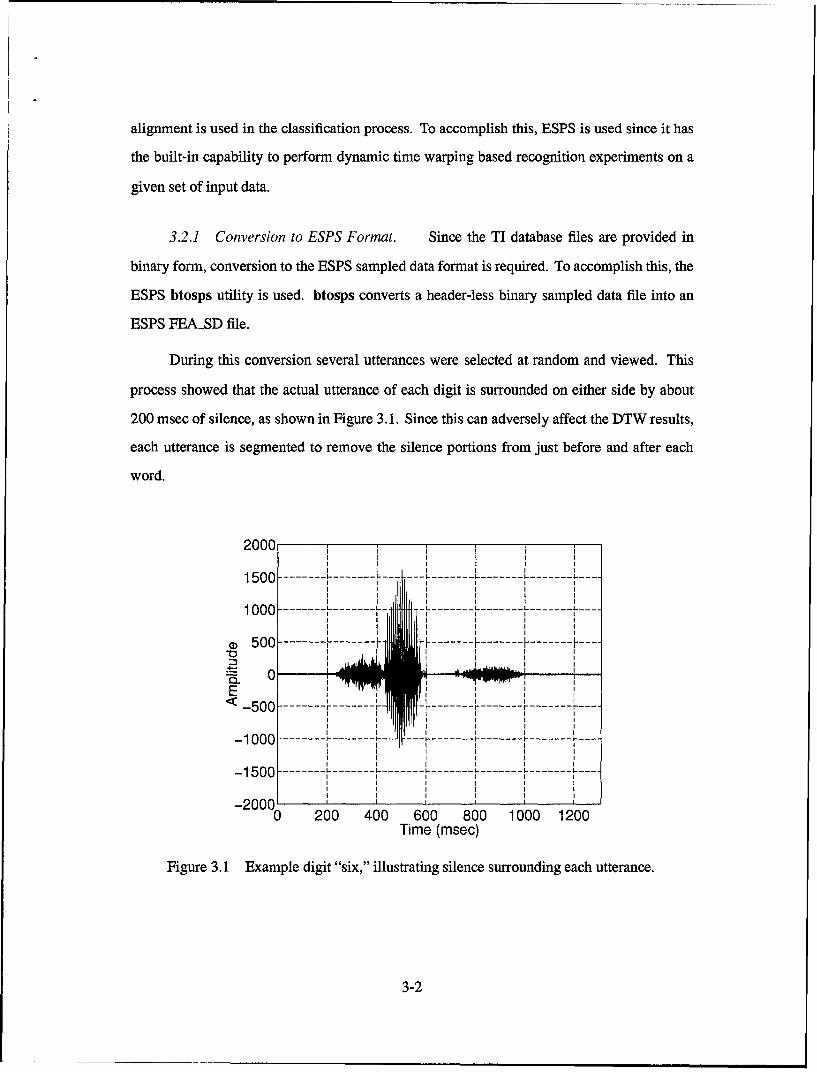
Figure 3.6 Segmentation by envelope detection: (a) Original utterance of the digit "six," (b)Absolute value of the utterance, (c) Envelope of the utterance (with threshold),(d) Segmented utterance.

A threshold was determined empirically, and applied to the envelope of each utterance

(see Figure 3.6 (c)). The starting point for a segmented utterance is located by the first breech

of the threshold by the envelope, and the stop point is marked by the second crossing.

3-8

Due to the large number of files, it is impractical to visually inspect segmentation

performance for the entire working database. However, by viewing about 100 examples,

this simple method proved to be adequate in obtaining a segmented utterance with which to

calculate the energy per interval as described above. Once the energies are computed, the total

energy per feature vector is normalized to one.

3.4 DTW with Critical Band Energy Features

To create a benchmark, experiments using dynamic time warping are conducted with

critical band energy features. These features are generated by omitting time averaging from

the critical band energy feature extraction method, and converting the resulting MATLAB files

to the ESPS format using the mat2fea utility. Thus, each matrix contained 9 rows representing

the number of critical bands, and a number of columns equal to the number of frames required

to cover the segmented utterance. Since dtw-rec considers one column of the input matrix

at a time, these features provide a valid set for comparison between the DTW results and the

results from experiments where time alignment is not used.

3.5 Concatenation of Feature Vectors

Another way to create feature sets is to concatenate previously generated features with

each other. Since the critical band energy and energy profile features were generated with

MATLAB, they were easily concatenated with another MATLAB routine. The procedure for

converting features created by ESPS is discussed below.

3.5.1 Averaged LPC and LPC Cepstral Features. A major premise of this work

is that each word may be represented by a single feature vector computed over the duration

of the word. The time-averaged critical band energy spectrogram is one such feature vector.

Jennings reports successfully using averaged LPC coefficients in an isolated digit recognition

task (4).

3-9

We are deeply indebted to Captain Dave Jennings for suggesting this unique approach,

and for providing the C code that performs the averaging and attaches a class label to each

vector. The procedure is to linearly average the LPC coefficients from each frame over the

word duration. A similar procedure is performed on the LPC cepstral coefficients. Typical

averaged LPC cepstral and LPC coefficients are show in Figures 3.7 and 3.8, respectively. A

copy of Jenning's code is provided in Appendix B.

3.6 Baseline Experiments/Dynamic Time Warping

Figure 3.9 illustrates the procedures involved in performing DTW classification using

the LPC cepstral feature set. A step by step procedure for obtaining the feature sets and

controlling the experiments for this work is provided in Appendix B.

3.6.1 List Preparation. With the data now ready for the dynamic time warping utility

dtw-rec, the final preparatory step is creating the lists necessary to control the experiments.

dtw-rec requires lists designating the training and testing templates for each pass through the

classification routine. For this work, the lists were set up to perform hold-one-out speaker-

independent recognition of the form used by (21).

With this method, the lists of reference templates (a series of LPC or LPC cepstral

vectors) each contain all the templates (from TI/train and TI/test) for each of the speakers

except the one to be classified. The test lists contain not only the test templates, but also the

training templates from the held out speaker. This method increases the size of the actual

training and testing sets, while providing speaker-independent classification. dtw-rec uses

the lists to pair up test and reference templates for distance measurements.

Having extracted the features and prepared the lists, the digits are classified using

dtw-rec. A single speaker-independent DTW experiment using all 16 speakers requires about

24 hours to complete. Once an experiment is completed, results are quantified by totaling the

number of digits classified, and computing the accuracies collectively, and on a per speaker

basis.

3-10

1.5

CU

a)S0.5

U-

0

-0.5 2 4 6 8 10 12

Index

Figure 3.7 Typical averaged 12th-order LPC cepstral features for ten utterances of the digit" zero."

3

2

(Dl

CO

U-- 1

-2-

2 4 6 8 10Index

Figure 3.8 Typical averaged 10th-order LPC coefficient features for ten utterances of the

digit "zero."

3-11

Frame SizeN= 150

Step Size w[n] p= 10f samp =12500 Hz M =75•- w •I

-Autocorr. )rm(s[n] Preemphasis Framing Windowing Analysis

Templates

Confusion Matrix cm(t) am(t)Confsio2M1wuanify =T LPC Param. LPC

Overall Accuracy] Results I I Conversion analysis

Figure 3.9 Typical processing steps for classification using DTW with the LPC cepstralfeature set.

To obtain the recognition accuracies for each digit, the number of correctly classified

digits is divided by the total number of digits classified for each digit. The result is multiplied

by 100, providing the percent accuracy for each digit.

Finally, the overall results are obtained by adding up the individual results and dividing

by ten. Confusion matrices for each experiment were generated by hand. These results are

used as a baseline against which the recognition rates for the other feature set and classifier

combinations are compared.

3.7 Recognition Without Time Alignment

The experiments in speaker-independent digit recognition without time alignment were

accomplished using LNKnet. LNKnet is a software environment that simplifies the application

of neural network, statistical, and machine learning pattern classification algorithms to new

databases (9).

Figure 3.10 shows a block diagram of the procedures involved in classifying the digits

using a multi-layer perceptron classifier with critical band energy features. The process is

similar for the other classifiers.

3.7.1 Experiments Using LNKnet. To determine the number of critical bands

resulting in the highest recognition accuracy for the LNKnet experiments, feature sets with

vectors containing 6, 9, 12, 15, 18, 21, and 24 elements are classified using Gaussian, multi-

3-12

samp Uniform Time f Critical Band

s[n] Spectrogram Average Freq. Average

Test Patterns A TrainingIndividual I <1!

Confusion MatrixC~nusin•Quantify I lvP • i9•MLP

Oveal Acuac l esults ; Classification \-- Training

Overall Accuracy Wit

Figure 3.10 Typical processing steps for classification using a MLP with the critical bandenergy feature set.

layer perceptron (MLP), and k-nearest neighbors (KNN) classifiers. The programs and step

by step procedures for performing these experiments are given in appendix B.

3.7.1.1 Gaussian Classifier. Gaussian classifiers are the simplest and most

common classifiers (9). The Gaussian classifier models each class with a Gaussian distribution

centered on the mean of that class. For this work, the variance was computed for each

class, using full covariance matrices with a minimum allowable variance of le-05. A priori

probabilities used during classification were computed from the training data using all of the

features.

3.7.1.2 Multi-layer Perceptron. Multi-layer perceptrons have been shown to

be useful for the digit recognition task (11). While LNKnet provides tremendous flexibility in

designing the structure of the MLP network, the same configuration is used for all experiments

in this work.

For these experiments, a two-layer perceptron with 25 hidden nodes is used. The number

of output nodes is set to ten (one for each digit), and the number of input nodes is determined

by the number of features per input feature vector. Gradient descent back propagation is used

to update the weights, with a step size of 0.1 and momentum equal to 0.6. The tolerance is

set such that back propagation is turned off if one of the outputs is within 0.01 of the desired

output. A squared error cost function and standard sigmoid nonlinearity are used, and the

3-13

weights are updated after each trial. Training is performed over 20 epochs, where each epoch

represents a single pass through the entire training set.

Several experiments are conducted using the MLP classifier. These experiments involve

both original and concatenated feature vectors. The theory behind the use of concatenated

feature vectors is that different types of features may have different strong points when

compared to each other.

For example, suppose critical band energies perform better in classifying male speakers

versus female speakers, or all the digits except twos and eights, whereas LPC cepstral features

perform well with female speakers and twos. By using multiple perspectives of each word,

one may be able to combine the benefits from each feature set, thereby classifying both male

and female speakers, and twos, with greater accuracy.

An example of an MLP classifier that combines three different feature sets for the digit

recognition task is shown in Figure 3.11. Given the nature of the training process where back

"One" "...Three" "Five" "Seven" "Nine""Two" "Four" "Six" "Eight" "...Ten"

InputII II

9 Critical Band 12 LPC Cepstral 10 LPCEnergy Coefficients Coefficients Coefficients

Figure 3.11 A MLP classifier that considers three different sets of features.

propagation is used, by introducing multiple feature sets at the MLP inputs, a sort of feature

3-14

fusion takes place. The different feature set combinations considered in this work are shown

below.

* Critical band energy and energy features

* Critical band energy and averaged LPC cepstral features

* Critical band energy and averaged LPC coefficient features

* Critical band energy, averaged LPC cepstral and LPC coefficient features

Experiments are completed using an MLP classifier and each of these feature sets for all 16

speakers, as well as for the male and female speaker sets individually.

3.7.1.3 k-Nearest Neighbors. According to (11), the KNN classifier performs

equal to or slightly better than the MLP for digit recognition. For this work, a KNN algorithm

with k = 1, and no cross-validation was used.

3.8 Quantifying the Results

In order to determine overall recognition rates, C-shells were written to gather the results

for each speaker and compute the overall accuracies. Confusion matrices are generated for

each experiment, and are presented in Chapter IV. All C-shells written to compile the results

are contained in appendix B.

3.9 Summary

To facilitate the continuance of this research we hope that the next group to take up this

effort can make use of, and improve upon, the ad hoc codes generated for this work. Several

conclusions that can be drawn from the actual experiments are listed below.

* When time alignment is used, words shall be segmented to eliminate silence preceding

and following an utterance.

* The DTW classifier with both critical band energy and LPC cepstral coefficients provides

a benchmark for testing new feature set/classifier combinations without time alignment.

3-15

" The time-averaged critical band energy feature set is used for initial experiments in

recognition without time alignment. The best number of bands is found empirically.

" Three classifiers are considered for initial classification of the critical band energy

features.

1. Gaussian.

2. MLP

3. KNN

"* The MLP is selected to exploit its inherent "feature fusion" capability.

"* Concatenated feature vectors are used to build new feature sets. The sets include

1. Critical band energy + energy profile.

2. Critical band energy + averaged LPC coefficients.

3. Critical band energy + averaged LPC cepstral coefficients.

4. Critical band energy + averaged LPC + averaged LPC cepstral coefficients.

3-16

11. Results

4.1 Introduction

This chapter discusses the results of the experiments detailed in Chapter H. For this

work, only speaker-independent recognition is considered, using the hold-one-out method

described in Chapter III, and in (15). Optimal feature length determination for the critical

band feature set is considered first. Comparisons are made between the recognition rates for

Gaussian, KNN, and MLP classifiers using several different vector lengths.

Three sets of experiments are conducted for most of the classifiers. These are male-only

recognition using the eight male speakers, female-only recognition using the eight female

speakers, and male-female recognition using the complete sixteen speaker set.

The results of the DTW experiments are introduced first, providing a baseline recog-

nition accuracy that is used as a goal for the experiments accomplished without using time

alignment. Features considered for the DTW experiments are 12th-order LPC cepstral coef-

ficients, and critical band energies.

Following the DTW experiments, results for the classifications without time alignment

are presented. The features sets considered in these experiments are the critical band energy,

averaged 12th-order LPC cepstral coefficients, averaged 10th-order LPC coefficients, and

energy profiles.

Several combinations of these feature sets are constructed by concatenation, and clas-

sified using a multi-layer perceptron. These combinations include the time-averaged critical

band energy features concatenated with the energy profile, averaged 12th-order LPC cepstral

coefficient, averaged 10th-order LPC coefficient, and averaged 12th-order LPC cepstral and

10th-order LPC coefficient features.

Statistical hypothesis testing is used to compare the DTW results with the results from

classifiers in which time-alignment is not used. The chapter is concluded by considering the

4-1

performance of the concatenated feature sets versus the critical band energy feature set with

the MLP classifier.

4.2 Optimum Feature Length Determination

To determine the optimum vector length for the critical band energy features described

in Chapter EI, several experiments were completed for three classifiers for vectors containing

6, 9, 12, 15, 18, 21, and 24 features. Figure 4.1 shows a plot of the recognition accuracy versus

the number of features for Gaussian, KNN, and MLP classifiers, using all sixteen speakers.

These experiments were repeated for the male-only and female-only speaker sets, yielding the

results shown in Figures 4.2 and 4.3.

While the accuracy for the MLP is slightly higher at eighteen elements versus nine in

Figure 4.1, all three classifiers show little or no improvement beyond nine elements. A similar

effect is seen for the male-only and female-only results of Figures 4.2 and 4.3.

78

76-

-. 74-

872

<70 -

68 ,, gauss+ knn

mip66-6 10 15 20 25

Number of Critical Bands

Figure 4.1 Comparison of recognition accuracy versus the number of elements per featurevector using both male and female speakers.

4-2

86

84-

-82

80-

<78

76 gauss

7+ 6n

m745 10 15 20 25

Number of Critical Bands

Figure 4.2 Comparison of recognition accuracy versus the number of elements per featurevector using male speakers only.

82

80

78

p--76-

874

°72

70m gauss

68 +g..* mlp1'0p

5 10 15 20 25Number of Critical Bands

Figure 4.3 Comparison of recognition accuracy versus the number of elements per featurevector using female speakers only.

4-3

Based on these results, it was determined that nine elements are sufficient for this feature

set. Thus, for all experiments involving the concatenation of vectors, nine-element critical

band energy feature vectors are used. Figures 4.1 through 4.3 also indicate that the MLP gives

the best results for the critical band energy feature set. Thus, the MLP is used to perform the

remaining experiments that do not involve time alignment.

Finally, since the male speaker recognition rate is substantially higher than the other

configurations (a phenomenon cited by (21) as common), results for this speaker set are

emphasized throughout this work.

4.3 Dynamic Time Warping

This section presents results from the dynamic time warping experiments. The ba-

sic experimental setup is discussed and confusion matrices and percent accuracy tables are

presented.

4.3.1 DTW Results Using LPC Cepstral Features. In the first DTW experiment,

12th-order LPC cepstral coefficients were used to classify the digits for both the male and

female speakers, yielding an overall recognition rate of 95.2%. This experiment was executed

to provide an idea as to what could be achieved using dynamic time warping. Table 4.1 shows

the confusion matrix for this experiment.

For this experiment, a short reference list was used for the distance computations.

Relative to a long list, a short reference list contains only one of ten possible templates for

each digit per each speaker. This was done to save time, since it took hours to complete a

DTW experiment.

For example, using a long list and a SPARC 20 work station, it took over 13 hours

to complete a speaker-independent experiment for just 8 of the 16 speakers! By reducing

the number of templates per digit per speaker from ten to one, the time required to run an

experiment was reduced to four or five hours for an eight speaker set.

4-4

Table 4.1 Confusion matrix for DTW classification using LPC cepstral features with bothmale and female speakers.

Computed DesiredClass Class

0 1 2 3 4 5 6 7 8 90 398 8 11 6 2 10 3 11 386 2 232 4 1 389 2 3 6 13 1 403 54 3 2 402 1 35 2 2 2 4 380 1 3 96 4037 8 1 10 2 4 405 28 3 4009 14 6 23 2 1 378

Total 410 415 415 414 414 414 414 416 416 414

Table 4.2 shows individual results for all sixteen speakers. There is a discrepancy here

in the number of results for speaker m5, versus the number for the rest of the experiments.

Apparently, for these features, the distance measurement for sample 08m5set9 (digit 8, male

speaker 5, session enrollment token 9) was outside the maximum distance allowed by dtw-rec.

Therefore, a distance measurement was not computed for this template. This did not occur

for any other experiments.

It is interesting to note that a visual inspection of this sample (and many others for m5)

shows that the plosive burst, or t is missing from this utterance, indicating poor enunciation

by the speaker.

4.4 DTW Results Using Critical Band Energy Features

To create an experiment that would provide a valid comparison with the non time-

alignment results from LNKnet, feature vectors were generated with elements obtained through

critical band frequency averaging of the spectrograms for each digit. Linear time averaging

was not used for this feature set. These features were applied to dtw-rec for classification.

4-5

Table 4.2 Overall results for DTW classification using LPC cepstral features with both male

and female speaker sets.

Speaker Classified Errors IAccuracy (%)fl 258 1 99.6f2 259 3 98.8f3 259 12 95.4f4 259 19 92.7f5 260 7 97.3f6 260 18 93.1f7 260 4 98.5f8 260 3 98.8

ml 260 13 95.0m2 260 2 99.2m3 260 6 97.7m4 256 0 100.0m5 255 17 93.3m6 258 12 95.4m7 257 10 96.1m8 260 70 73.1

Total 4141 J 197 95.2

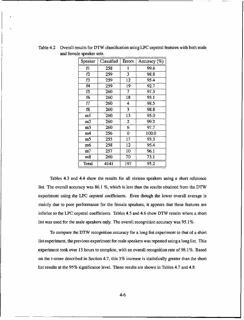
Tables 4.3 and 4.4 show the results for all sixteen speakers using a short reference

list. The overall accuracy was 86.1 %, which is less than the results obtained from the DTW

experiment using the LPC cepstral coefficients. Even though the lower overall average is

mainly due to poor performance for the female speakers, it appears that these features are

inferior to the LPC cepstral coefficients. Tables 4.5 and 4.6 show DTW results where a short

list was used for the male speakers only. The overall recognition accuracy was 95.1%.

To compare the DTW recognition accuracy for a long list experiment to that of a short

list experiment, the previous experiment for male speakers was repeated using a long list. This

experiment took over 13 hours to complete, with an overall recognition rate of 98.1%. Based

on the t-score described in Section 4.7, this 3% increase is statistically greater than the short

list results at the 95% significance level. These results are shown in Tables 4.7 and 4.8.

4-6

Table 4.3 Confusion matrix for DTW classification using critical band energy features anda short reference list with both male and female speaker sets.


0 1 2 3 4 5 6 7 8 90 359 23 1 2 11 13 1 111 4 299 4 37 5 122 15 2 374 79 4 29 3 173 15 2 38 324 3 1 10 94 10 11 392 2 9 15 14 2 340 25

6 .1 2 357 87 11 1 384 18 1 5 25 3809 7 53 2 35 1 355

Total 410 415 415 414 414 414 414 416 416 414

Table 4.4 Overall results for DTW classification using critical band energy features and ashort reference list with both male and female speaker sets.

Speaker Classified Errors Accuracy (%)fl 258 27 89.5f2 259 41 84.2f3 259 68 73.8

f4 259 88 66.0f5 260 67 74.2f6 260 71 72.7

V 260 34 86.9f8 260 81 68.8ml 260 7 97.3m2 260 11 95.8m3 260 24 90.8m4 256 18 93.0m5 256 14 94.5m6 258 10 96.1m7 257 10 96.1m8 260 7 97.3

Total [ 4142 1 578 86.1

4-7

Table 4.5 Confusion matrix for DTW classification using critical band energy features anda short reference list with male speakers only.


0 1 2 3 4 5 6 7 8 90 202 1 21 189 1 2

2 3 202 7 83 4 193 1 5 4

4 2 2045 1 199 226 204 47 11 1 207 18 1 4 1 1919 2 3 2 7 1 175

Total 203 208 208 208 208 208 208 208 208 208

Table 4.6 Overall results for DTW classification using critical band energy features and a

short reference list with male speakers only.

Speaker Classified Errors Accuracy (%)ml 260 7 97.3m2 260 11 95.8m3 260 24 90.8m4 256 18 93.0m5 256 14 94.5m6 258 10 96.1m7 257 10 96.1m8 260 7 97.3

Total I 2067 101 [ 95.1

4-8

Table 4.7 Confusion matrix for DTW classification using critical band energy features anda long reference list with male speakers only.


0 1 2 3 4 5 6 7 8 90 2031 206 32 3 197 23 7 202 1 14 206 45 203 96 2 2047 2078 1 2 1 2089 2 1 3 193

Total 203 208 208 208 208 208 208 208 208 208

Table 4.8 Overall results for DTW classification using critical band energy features and along reference list with male speakers only.

Speaker Classified Errors Accuracy(%)ml 260 5 98.1m2 260 3 98.8m3 260 13 95.0m4 256 3 98.8m5 256 7 97.3m6 258 2 99.2m7 257 0 100.0m8 260 6 97.7

Total 2067 j 39 j 98.1

4-9

4.5 Results For Recognition Without Time Alignment

This section contains the results from all experiments accomplished without using time

alignment. The classifiers used for these experiments are the multi-layer perceptron, k-nearest

neighbors, and Gaussian.

The first experiment was accomplished using the critical band energy features. Note

that these features take the form of one vector per word versus numerous (usually more than

100) vectors per word for the DTW experiments. This represents a tremendous savings in

storage space for this procedure.

These experiments were followed by classification of the energy profile vectors, aver-

aged LPC cepstral features, averaged LPC coefficient features and various combinations of

these features.

4.5.1 Critical Band Energy Feature Classification. A confusion matrix for the

nine-element critical band feature set using all sixteen speakers with an MLP classifier is

shown in Table 4.9. Individual results for each speaker are given in Table 4.10. Similar results

for the KNN and Gaussian classifiers are provided in Appendix A. The overall recognition

accuracy for this experiment is 76.2%.

4.5.1.1 Best Results for Critical Band Features. As indicated in Figure 4.2,

the highest recognition accuracy for the MLP classifier using critical band energy features was

obtained for the male-only experiment. The confusion matrix and individual speaker results

for this experiment are shown in tables 4.11 and 4.12, respectively. The overall accuracy for

this configuration was 84.7%.

4.5.2 Results Using Concatenated Feature Vectors. In an attempt to improve the

MLP classifier accuracy, experiments were conducted with various concatenated feature sets in

which the original critical band energy features were kept, with different features concatenated

to them. Before concatenation, each feature set to be included with the critical band features

was classified by itself. In no instance did these other features provide a higher accuracy than

4-10

Table 4.9 Confusion matrix for the MLP classifier using critical band energy features for

both the male and female speakers with nine-element feature vectors.


0 1 2 3 4 5 6 7 8 90 288 6 5 22 2 1 1 27 1 111 4 283 1 14 19 5 312 20 11 239 69 4 2 23 43 152 286 4 194 19 30 393 2 1 25 55 4 367 3 526 4 3 6 336 28 66 37 17 3 1 1 4 6 339 3 158 1 13 29 66 3 3259 14 27 2 1 21 5 300

Total 410 415 415 414 414 414 414 416 416 414

Table 4.10 Overall results for the MLP classifier with critical band energy features for boththe male and female speakers using 9-element feature vectors.

Speaker Classified Errors Accuracy (%)

fl 258 71 72.5f2 259 74 71.4B 259 66 74.5f4 259 104 59.8f5 260 73 71.9f6 260 67 74.2P7 260 52 80.0f8 260 47 81.9ml 260 97 62.7m2 260 48 81.5

m3 260 36 86.2m4 256 16 93.8m5 256 75 70.7m6 258 41 84.1m7 257 54 79.0m8 260 65 75.0

Total j 4142 [ 986 76.2

4-11

Table 4.11 Confusion matrix for the MLP classifier with critical band energy features formale speakers only using 9-element feature vectors.


0 1 2 3 4 5 6 7 8 90 176 19 1 2 31 1 191 9 4 2 182 1 175 19 3 23 20 30 165 2 6 14 11 197 1

5 3 190 40

6 1 174 25 21 37 1 1 7 173 98 5 3 3 19 1759 2 2 11 6 135

Total 207 207 207 206 206 206 206 208 208 206

Table 4.12 Overall results for the MLP classifier with critical band energy features for malespeakers only using 9-element feature vectors.

Speaker Classified Errors J Accuracy (%)ml 260 53 79.6m2 260 38 85.4m3 260 28 89.2m4 256 21 91.8m5 256 50 80.5m6 258 15 94.2m7 257 66 74.3m8 260 45 82.7

Total 2067 3161 84.7

4-12

the critical band energy features alone. The results of these individual experiments are given

in Appendix A.

4.5.2.1 Critical Band Energy and Energy Profile Features. The first con-

catenated feature set contained the critical band energy features and features obtained by

computing the energy in nine equal-duration segments spread across the length of each utter-

ance. The energy computations were detailed in Chapter III. As shown in Appendix A, this

experiment resulted in a slight increase in recognition accuracy (from 84.7% to 85.9%) for the

male speaker set.

4.5.2.2 Critical Band Energy and Averaged LPC Coefficients. The next

feature set consists of the critical band energy features concatenated with averaged 10th-order

LPC coefficients. These feature vectors contain 19 elements.

The confusion matrix for the male speaker set is shown Table 4.13. As Table 4.14

shows, this experiment results in a recognition rate of 94.1%. The tables for the female and

male-female experiments, contained in Appendix A, indicate recognition rates of 86.2% and

88.4%, respectively.

4.5.2.3 Critical Band Energy and Averaged LPC Cepstral Coefficients. The

third feature set consists of the critical band energy features concatenated with averaged

12th-order LPC cepstral coefficients. These feature vectors contain 21 elements.

The confusion matrix for the male speaker set is shown in Table 4.15. As Table 4.16

shows, this experiment results in a recognition accuracy of 94.6%. The tables for the female

and male-female experiments, contained in Appendix A, indicate recognition accuracies of

86.5% and 89.0%, respectively.

4.5.3 Critical Band Energy, Averaged LPC Cepstral, and LPC Features. The last

feature set considered consists of the critical band energy features combined with both the

4-13

Table 4.13 Confusion matrix for MLP classification using concatenated critical band energy

and averaged 10th-order LPC coefficient features for male speakers only.


0 1 2 3 4 5 6 7 8 9

0 192 3 2 26 1 1 31 1 193 2 2 162 2 202 1 13 8 3 176 14 7 2045 1 201 12

6 1 203 10 17 1 1 3 1968 1 3 1 205 19 1 3 2 173

Total 207 207 207 206 206 206 206 208 208 206

Table 4.14 Overall results for MLP classification using concatenated critical band energy

and averaged 10th-order LPC coefficient features for male speakers only.Speaker Classified [Errors I Accuracy (%)

ml 260 18 93.1

m2 260 9 96.5m3 260 25 90.4m4 256 0 100.0m5 256 35 86.3m6 258 8 96.9

m7 257 12 95.3m8 260 15 94.2

Total 2067 122 94.1

4-14

Table 4.15 Confusion matrix for MLP classification using concatenated critical band energy

and averaged 12th-order LPC cepstrum features for male speakers only.


0 1 2 3 4 5 6 7 8 90 196 10 1 1 1 31 191 1 10

2 6 1 191 5 13 2 4 197 1 14 6 206 15 1 200 8 76 205 4 27 1 1 1 1 189 78 2 1 2 1 2049 . 9 4 4 177

Total 207 207 207 206 206 206 206 208 208 206

Table 4.16 Overall results for MLP classification using concatenated critical band energyand averaged 12th-order LPC cepstrum features for male speakers only.


Total 2067 111 [ 94.6

4-15

averaged 12th-order LPC cepstral coefficients and averaged 10th-order LPC coefficients. The

resulting feature vectors contain 31 elements.

The confusion matrix for the male speaker set is shown in Table 4.17. Table 4.18

indicates a recognition accuracy of 97.1% for this experiment. This represents an improvement

from 84.7% to 97.1%, or 12.4%, as compared to the results obtained using the critical band

energy features alone.

Table 4.17 Confusion matrix for MLP classification using concatenated critical band energy,averaged LPC cepstrum, and averaged LPC coefficient features for male speakersonly.


0 1 2 3 4 5 6 7 8 90 203 5 31 1 201 14

2 2 202

3 1 202 1 24 1 206 1

5 205 1 11

6 206 8 17 1968 1 206

9 5 1 2 179

Total 207 207 207 206 206 206 206 208 208 206

4.6 Accuracy Comparison for Various Feature Sets

Table 4.19 provides a comparison of the recognition accuracies achieved for the various

feature set configurations. For the chosen combinations, the accuracy improves as the number

of different features is increased. This supports the theory that recognition rates can benefit

from multiple perspectives of a word, especially when MLP classifiers are used.

4-16

Table 4.18 Overall results for MLP classification using concatenated critical band energy,averaged LPC cepstrum, and averaged LPC coefficient features for male speakersonly.

Speaker IClassifiedI Errors I Accuracy (%)

ml 260 10 96.2m2 260 2 99.2m3 260 7 97.3m4 256 3 98.8m5 256 23 91.0m6 258 0 100.0m7 257 7 97.3m8 260 9 96.5

j Total [ 2067 1 61 j 97.1

Table 4.19 Comparison of MLP recognition accuracy for the original critical band energyfeatures and the various concatenated feature sets.

Feature Male Female Male-FemaleSet % Accuracy % Accuracy % Accuracy

Critical Band Energy 84.7 77.9 76.2LPC Features 79.4 74.9 74.4

Energy Profile Features 61.0 - -

Cepstral Features 78.4 74.5 69.7Critical Band/Energy 85.9 - -

Critical Band/LPC 94.1 88.2 88.4Critical Band/LPC Cepstrum 94.6 86.5 89.0

Critical Band/LPC Cepstrum/LPC 97.1 89.1 92.4

4-17

4.7 Statistical Hypothesis Testing

In order to compare the DTW results with those from the MLP classifier, one can look

at the statistical significance of the accuracy differences. Using the results for male speakers

only, there are eight speakers to consider for each experiment.

Table 4.20 shows the per-speaker accuracy for the best MLP results, and the short and

long list DTW results. To determine whether or not DTW and the MLP have a statistically

significant difference in average recognition rates, the t-score is computed as

t n - 1(d[i] - m[i]) (4.1)

where i = 1,... ,8, and d[i] and m[i] are the percent accuracy results for speaker i for the

DTW and MLP classifiers, and Sd is the sample standard deviation of the paired differences,

and n is the number of pairs.

In these experiments, the paired differences have a t distribution with seven degrees

of freedom (3). Under these conditions, a t-score greater than 1.895 indicates that the DTW

recognition rate is greater than the MLP rate at the 95% significance level. A t-score less than

-1.895 indicates that the DTW recognition rate is less than the MLP at the 95% significance

level (19).

The t-score for the MLP v.s. long list comparison is t = 1.1537, indicating no statistical

difference for the DTW recognition rate versus the MLP. The t-score for the MLP versus

the short list DTW comparison is t = -1.5266. Thus, for a short DTW reference list there is

again no statistical difference between the accuracy of dynamic time warping versus the MLP

classifier. Table 4.20 also includes the overall accuracy and 95% confidence interval for each

of the methods.

These results are impressive, considering that it takes over thirteen hours to complete

the long-list DTW experiment for eight speakers, over 3 hours to complete the short-list DTW

experiment, and only a few minutes to complete the MLP experiment. Table 4.21 shows

individual speaker accuracies for all sixteen speakers for the short list DTW experiment and

4-18

Table 4.20 Per speaker recognition accuracies for male speakers only. The confidenceinterval for the overall results is 95%.

Speaker % AccuracyMLP DTW Short DTW Long

ml 96.2 97.3 98.1m2 99.2 95.8 98.8m3 97.3 90.8 95.0m4 98.8 93.0 98.8m5 91.0 94.5 97.3m6 100.0 96.1 99.2m7 97.3 96.1 100.0m8 96.5 97.3 97.7

Overall 97.1 ± 2.3 95.1 ± 1.9 98.1 ± 1.3

Table 4.21 Per speaker recognition accuracies for both male and female speaker sets. Theconfidence interval for the overall results is 95%.

Speaker % AccuracyMLP DTW Short

fl 89.9 99.6f2 96.5 98.803 96.9 95.4f4 79.9 92.7f5 91.5 97.3f6 90.8 93.1V 90.8 98.5f8 93.8 98.8ml 75.8 95.0m2 98.1 99.2m3 95.8 97.7m4 99.6 100.0m5 87.9 93.3m6 97.7 95.4m7 98.8 96.1m8 94.6 73.1

Overall 92.4 ± 3.6 95.2 ± 3.4

4-19

the MLP using the concatenated critical band energy, averaged 12th-order LPC cepstral, and

averaged 10th-order LPC coefficient feature set.

For these data, the t-score is t = 1.3065. Again, there is no statistically significant

difference between the recognition rates of the two classifiers. However, it should be noted

that this is not a completely fair test since there were fewer reference templates (due to the

short reference lists) for the DTW classifier than there were training samples for the MLP. The

overall accuracy and confidence interval for both methods is also shown in Table 4.21.

4.8 Performance Breakdown

One possible question, given these results, is "how can such a dramatic improvement in

the recognition rate be achieved by concatenating three feature sets that perform rather poorly

on an individual basis?" To try to answer this question, consider Tables 4.22, through 4.25.

These tables give a digit by digit synopsis of the performance of each speaker for the

three sets of features used to get the best results for the male speaker set. Table 4.22 shows

the individual results that combine to yield a 97.1% recognition rate. The two digits with the

highest error rates are seven and nine. In fact, nearly 40% of the errors for this experiment

can be attributed to speaker ml uttering the digit "seven" and speaker m5 uttering the digit

"nine." From the confusion matrix (see Table 4.17), it is apparent that "seven" is most often

confused with "six," whereas "nine" is most often confused with "one" and "five."

Considering Tables 4.23 through 4.25, insight is gained as to what occurs. In general,

utterances of the digit nine by speaker m5 are not well recognized for any of the feature sets,

and the combined feature sets seem unable to improve the overall results for this speaker-digit

combination.

However, the digit seven results for the critical band energy features show only four

errors for speaker ml versus for the combined features. It seems possible that the 23 errors

resulting with the LPC cepstral features somehow hampers the ability of the combined feature

sets to provide substantial improvement.

4-20

Table 4.22 Error synopsis for male-only speaker-independent recognition using concate-nated critical band energy, LPC cepstral, and LPC coefficient features.

Digit Number of ErrorsSpoken Per Speaker

ml [ m2] m3 I m4 m5 I m6 I m7 [ im78l Totals

zero 0 0 1 0 0 0 3 0 4one 0 0 1 0 0 0 1 4 6two 0 0 0 0 0 0 0 5 5

three 0 0 1 0 3 0 0 0 4four 0 0 0 0 0 0 0 0 0five 0 0 0 0 0 0 1 0 1six 0 0 0 0 0 0 0 0 0

seven 7 0 1 1 2 0 1 0 12eight 1 0 0 0 1 0 0 0 2nine 23 2 17 0 1 0 27

Totals 10 2 7 3 23 0 7 9 61

Table 4.23 Error synopsis for male-only speaker-independent recognition using the criticalband energy features.


mlm21 m3 m4[m5Im6 m7Im8 11Totalszero 2 1 1 0 0 6 19 2 31one 0 0 3 0 10 1 1 1 16two 3 0 1 0 0 1 10 17 32


seven 4 0 0 5 0 1 17 8 35eight 15 9 0 2 1 0 0 6 33nine 24 23 4 0 14 0 2 4 71

Totals 53 38 28 21_1 50 15 66 45 -316

4-21

Table 4.24 Error synopsis for male-only speaker-independent recognition using the LPCcepstral features.


_ _ml m2 [ m3 I m4 1m5 1 m6 I m7 I m8 11 Totals

zero 22 26 20 1 1 15 11 2 98one 0 0 1 4 15 12 15 11 58two 24 15 4 1 23 1 3 26 97


seven 23 1 3 0 9 1 9 0 46eight 7 1 0 0 2 0 0 1 11nine 1 0 6 4 25 1 14 3 54

Totals 85 50 43 15 101 39 66 47 446

Table 4.25 Error synopsis for male-only speaker-independent recognition using the LPCcoefficient features.


ml m2 m3 m4] m5 I m6 [m7 Im8 Totals

zero 15 4 6 7 5 11 19 8 75one 3 1 6 0 4 4 1 13 32two 11 25 16 5 6 1 6 14 84


seven 7 4 3 7 14 6 0 1 42eight 5 0 7 0 6 0 1 0 19nine 19 0 5 3 18 5 3 1 54

Totals 72 1 58 53 25 85 51 31 5011 425

4-22

Yet, this type of result pertains to only a few of the 80 combinations shown in Table 4.22.

Specifically, there are only 4 of 80 speaker-digit combinations where performance is worse for

the combined feature set versus the critical band energy features, and only 3 of the remaining

76 cases where the performance is the same. Thus, the recognition rate is improved for 73 out

of 80 speaker-digit combinations.

Tables 4.23 through 4.25 also show that the combined feature set performs better on

all digits across all speakers when compared with the individual feature sets. Through this

analysis, the MLP is seen to perform feature fusion, improving upon the best features from

each individual feature set, for each digit.

4.9 Conclusions

From the results given in this chapter, one can conclude that for speaker-independent

recognition of male speakers, an MLP classifier can achieve results statistically equal to

classifiers using dynamic time warping.

The recognition rates for both the male and female speakers are also shown to be

statistically equivalent for a shortened list of reference templates for the DTW classifier versus

an MLP classifier. Therefore, recognition accuracies equal to those obtainable with DTW can

be achieved with the MLP.

These results also show that the MLP can be used to perform feature fusion when several

different feature sets are presented at the inputs to the classifier. Even though the feature sets

considered in this work are newly developed, they are based on well known parameters. The

results given in this chapter support the hypothesis that high accuracy speech recognition is

possible without performing time alignment.

4-23

V Conclusions and Recommendations

5.1 Conclusions

The goals of this research are to find feature sets for speech recognition that perform

well without using time alignment, and to identify classifiers that provide good performance

with these features. Using the digits from the T146 database, baseline speaker-independent

recognition rates of 95.2% for the complete speaker set, and 98.1% for the male speaker set,

are established using dynamic time warping.

Energies for a selected number of critical bands covering 300 to 3000 Hz were computed

from time-averaged spectrograms of the digits. These features performed poorly by themselves

in experiments without time alignment using an MLP classifier.

Other features considered in this work include linearly averaged LPC and LPC cepstral

coefficients. While these additional features also performed poorly on an individual basis, by

concatenating them with the original time-averaged critical band energy features recognition

accuracy was dramatically improved.

For the male speaker subset, there was no statistical difference between the recognition

rates using DTW and those using the MLP with no time alignment. These results support

further research into speech recognition without time alignment.

5.2 Accomplishments

Through this work, the following objectives were successfully accomplished:

Feature sets were found that perform well in the digit recognition task without the need

for time alignment of the data. All experiments were conducted using the hold-one-out

method for speaker-independent recognition, and telephone bandwidth (300 - 3000 Hz)

critical band energy features.

1. 94.1% accuracy was achieved for the male speaker set using concatenated critical

band energy and averaged LPC coefficient features.

5-1


band energy and averaged LPC cepstral features.


band energy, and averaged LPC cepstral and LPC coefficient features.

4. 92.4% accuracy was achieved for the complete male and female speaker set using

concatenated critical band energy, and averaged LPC cepstral and LPC coefficient

features.

5.3 Recommendations

Considering the accuracies obtained by Lippmann (11), and by Shore and Burton (21),

as well as the results from this work, there is enough evidence to support further research

into obtaining alternative feature sets for speech recognition without time alignment. Due

to time limitations, an extensive search for new feature sets was not completed here. Some

suggestions for carrying on this work include:

"* Further consideration of new feature sets.

"* Continue looking at combinations of existing features as new feature sets.

"* Analysis of the strengths of individual feature sets and classifiers.

5.3.1 Expanding the Vocabulary. Given the successful performance of the features

generated for this work on the digit recognition task, and the interest in voice recognition for

limited vocabulary applications such as the cockpit vocabulary studied by (16), extending the

vocabulary to the complete T146 database should be considered.

5.3.2 Performance in Noise. Since this is a crucial consideration for many military

applications, a comprehensive analysis of the effects of noise should be considered in future

research.

5-2

5.3.3 How Does It Work? An interesting aspect of the results obtained from this

work are the individual results for each speaker that combine to give the overall results. While

this was briefly analyzed in Chapter IV, there are still many open questions in this area. One

area to consider is:

9 Is there a mathematical basis for why the averaged LPC and LPC cepstral coefficients

add useful information to the critical band energy feature set?

5.3.4 Real-time Recognizer. Since the structure of the MLP with multiple identical

elements is compatible with current VLSI technology, the possibility of creating a real-time

word recognizer seems reasonable. The ETANN chip discussed in (2) is available with 128

trainable "neurons," which is enough to reproduce the software MLP used in this work. Since

the chip is trainable, new feature sets could be tested with such a system.

5-3

Appendix A. Experimental Results

A.1 Introduction

This appendix contains experimental results generated by this work that do not directly

contribute to the overall conclusions. Confusion matrices and individual speaker accuracies are

briefly discussed. This material is presented to provide a complete package of all experimental

results obtained from this work.

By file name, the 18 files missing from the testing data set provided for this work are

00flsltO, 00flsltl, OOf2sltO, OOf3sltO, OOf4sltO, 00m4s4tl, 04m4s8t0, 05m4s7t0, 09m4s5t1,

02m5s4t1, 04m5s6t1, 06m5s2tl, 09m5sltO, 03m6s4tl, 05m6s4t1, Olm7s4tl, 03m7s4t1, and

06m7s7t0.

A.2 Classifier Accuracy Comparison

To determine the optimum number of features per feature vector, experiments were

completed for 6, 9, 12, 15, 18, 21, and 24 element feature vectors. Plots of recognition

accuracy versus the number of features are shown in Chapter IV.

Figures A. 1, A.2, and A.3 show, in tabular form, the recognition accuracies obtained for

the MLP, KNN, and Gaussian classifiers. Based on these results, it is determined that nine-

element feature vectors are sufficient when considering time-averaged critical band energies.

The tables also indicate that the MLP classifier gives the best results for the critical band

energy feature set.

A.3 Results For Individual Feature Sets

This section contains the classification results for each feature set considered before

concatenations are performed. Confusion matrices and individual speaker results are provided,

with a brief discussion of each.

A-1

Table A. 1 MLP classifier accuracy per number of features for male, female, and completespeaker sets using critical band energy features.

Number of Overall Accuracy Overall Accuracy Overall AccuracyFeatures Male (%) Female (%) Both (%)

6 79.40 74.88 71.869 84.71 77.93 76.2112 85.30 80.82 75.7715 84.73 80.04 75.6318 84.44 79.85 77.1221 83.81 78.98 75.5824 85.25 78.44 74.08

Table A.2 KNN classifier accuracy per number of features for male, female, and completespeaker sets using critical band energy features.


6 74.76 66.59 67.739 81.38 72.33 74.3412 81.21 72.23 75.0015 82.41 71.51 74.8018 82.84 71.85 75.0521 82.27 70.16 74.4224 84.01 71.60 75.08

Table A.3 Gaussian classifier accuracy per number of features for male, female, and com-plete speaker sets using critical band energy features.


6 79.74 72.81 69.739 82.22 76.23 75.25

12 82.03 73.97 72.9615 80.44 75.12 71.7818 80.84 73.97 71.1521 80.89 72.86 70.0724 80.79 71.76 69.49

A-2

A.3.1 Critical Band Energy Feature Set. Tables A.4 and A.5 show the results for the

female speaker set for the MLP classifier, using critical band energy features. The confusion

matrices for the nine-element KNN and Gaussian classifier results for the complete feature

set, the male speaker set, and the female speaker set are shown in even numbered tables A.6

through A. 16, while the individual speaker results are shown in odd numbered tables A.7

through A. 17.

The overall recognition rate for the MLP classifier for the female speaker set is 77.93%.

The overall recognition rates for the complete speaker set for the KNN and Gaussian classifiers

are 74.34% and 75.25%, respectively. Results for the male speaker set are 81.38% for the

KNN classifier and 82.22% for the Gaussian classifier, and results for the female speaker set

are 72.33% for the KNN classifier and 76.23% for the Gaussian classifier.

Table A.4 Confusion matrix for the MLP classifier using critical band energy features forthe female speaker set.


0 1 2 3 4 5 6 7 8 90 147 2 6 5 6 4 1 41 155 2 15 182 14 11 103 64 11 2 13 10 93 1274 19 4 199 15 1 26 1 176 146 5 11 178 2 307 4 1 1 3 190 2 28 2 27 1739 6 10 1 16 169

Total 203 208 208 208 208 208 208 208 208 208

A-3

Table A.5 Overall results for the MLP classifier using critical band energy features for thefemale speaker set.

Speaker I Classified I Errors Accuracy (%)fi 258 57 77.91f2 259 41 84.17f3 259 39 84.94f4 259 104 59.85f5 260 75 71.15f6 260 59 77.31f7 260 40 84.62f8 260 43 83.46

Total 2075 j 458 j 77.__93

Table A.6 Confusion matrix for the KNN classifier using critical band energy features forboth the male and female speakers using 9-element feature vectors.


0 1 2 3 4 5 6 7 8 90 297 8 18 50 4 3 16 3 121 8 315 0 18 22 4 462 13 1 273 90 3 7 83 55 107 240 2 2 18 124 8 18 387 2 35 42 2 348 1 546 6 5 11 314 25 85 37 5 2 3 1 2 1 12 337 3 178 12 9 20 1 79 7 299 19 6 29 2 41 1 14 269

Total 410 415 415 414 414 414 414 416 416 414

A-4

Table A.7 Overall results for the KNN classifier using critical band energy features for boththe male and female speakers using 9-element feature vectors.

Speaker [ Classified Errors Accuracy(%)

fl 258 108 72.48f2 259 49 71.43f3 259 61 74.52f4 259 131 59.85f5 260 84 71.92f6 260 82 74.23f7 260 42 80.00f8 260 50 81.92ml 260 75 62.69m2 260 41 81.54m3 260 59 86.15m4 256 31 93.75m5 256 66 70.70m6 258 57 84.11m7 257 49 78.99m8 260 78 75.00

Total 4142 j 1063 74.34

Table A.8 Confusion matrix for the KNN classifier using critical band energy features forthe male speaker set.


0 1 2 3 4 5 6 7 8 90 56 6 14 32 68 39 4 15 4 101 4 72 10 11 5 13 3 3 7 562 17 22 94 15 18 14 3 213 46 31 33 87 47 13 43 19 414 51 11 19 26 50 50 1 8 5 195 3 7 9 8 11 14 3 2 156 2 2 2 150 6 22 27 22 15 16 12 5 12 18 111 5 118 4 21 5 2 3 19 5 139 119 5 21 6 13 12 2 22

Total [-207 207 207 206 206 206 206 208 208 206

A-5

Table A.9 Overall results for the KNN classifier using critical band energy features for themale speaker set.

Speaker Classified [ Errors Accuracy (%)

ml 260 61 76.54m2 260 32 87.69m3 260 47 81.92m4 256 28 89.06m5 256 61 76.17m6 258 39 84.88m7 257 42 83.66m8 260 75 71.15

Total 2067 385 81.38

Table A. 10 Confusion matrix for the KNN classifier using critical band energy features forthe female speaker set.


0 1 2 3 4 5 6 7 8 90 151 7 3 15 3 2 2 2 81 3 133 7 26 262 7 113 75 3 9 2 23 21 82 96 1 54 7 13 197 45 38 1 171 1 176 1 7 10 158 8 33 17 2 2 1 5 168 5 18 9 1 12 39 14 1619 2 17 10 2 153

Total 203 208 208 208 208 208 208 208 208 208

A-6

Table A. 11 Overall results for the KNN classifier using critical band energy features for thefemale speaker set.

Speaker Classified J Errors I Accuracy (%)fl 258 92 64.34f2 259 46 82.24f3 259 59 77.22f4 259 115 55.60f5 260 83 68.08f6 260 80 69.23f7 260 41 84.23f8 260 58 77.69

Total 2075 574 72.33

Table A. 12 Confusion matrix for the Gaussian classifier using critical band energy featuresfor both the male and female speakers using 9-element feature vectors.


0 1 2 3 4 5 6 7 8 90 308 7 12 16 2 5 3 28 20 211 8 279 1 27 48 2 1 352 4 312 78 8 4

3 60 74 295 13 184 1 39 378 15 1 31 5 326 2 316 1 . 2 4 293 11 55 37 9 1 6 1 22 299 5 108 7 8 2 75 56 3129 18 58 1 13 33 18 1 314

Total 410 415 415 414 414 414 414 416 416 414

A-7

Table A. 13 Overall results for the Gaussian classifier using critical band energy features forboth the male and female speakers with 9-element feature vectors.

Speaker Classified Errors I Accuracy (%)]

fl 258 108 72.48f2 259 49 71.43f3 259 61 74.52f4 259 131 59.85f5 260 84 71.92f6 260 82 74.23f7 260 42 80.00

f8 260 50 81.92ml 260 75 62.69m2 260 41 81.54m3 260 59 86.15m4 256 31 93.75m5 256 66 70.70m6 258 57 84.11m7 257 49 78.99m8 260 78 75.00

Total 4142 1026 j 75.25

Table A. 14 Confusion matrix for the Gaussian classifier using critical band energy featuresfor the male speaker set.


0 1 2 3 4 5 6 7 8 90 163 1 11 1 3 10 10 21 4 183 9 2 3 102 162 15 73 33 33 180 2 84 6 1925 5 4 183 1 406 1 159 15 21 37 3 2 1 21 164 78 4 13 1699 4 13 4 1 19 1 15 144

Total 207 207 207 206 206 206 206 208 208 206

A-8

Table A. 15 Overall results for the Gaussian classifier using critical band energy features forthe male speaker set.

Speaker Classified Errors Ac~curacy(%)

ml 260 88 66.15m2 260 31 88.08m3 260 48 81.54m4 256 25 90.23m5 256 41 83.98m6 258 19 92.64m7 257 58 77.43m8 260 58 77.69

Total 2067 368 82.22

Table A. 16 Confusion matrix for the Gaussian classifier using critical band energy featuresfor the female speaker set.


0 1 2 3 4 5 6 7 8 90 179 3 10 2 3 12 12 61 131 5 9 3 312 6 131 55 9 2 13 10 73 139 7 34 3 11 197 2 15 39 177 1 296 1 4 144 5 197 1 2 3 1 5 176 5 28 40 5 1689 4 24 1 1 19 3 140

Total 203 208 208 208 208 208 208 208 208208

A-9

Table A. 17 Overall results for the Gaussian classifier using critical band energy features forthe female speaker set.

Speaker [Classified Errors Accuracy (%)

fl 258 75 70.93f2 259 42 83.78f3 259 67 74.13f4 259 100 61.93f5 260 67 74.23f6 260 68 73.85f7 260 26 90.00f8 260 48 81.54

Total [ 2075 1 493 j 76.23

A-10

A.3.2 Energy Profile Feature Set. Tables A. 18 and A. 19 show the confusion matrix

and individual speaker results for the male speaker set for MLP classification of the energy

profile feature set. The overall recognition accuracy is 38.99%. There are no results for the

female and complete speaker sets.

Table A. 18 Confusion matrix results for the MLP classifier using energy profile features forthe male speaker set.


0 1 2 3 4 5 6 7 8 90 56 6 14 32 68 39 4 15 4 101 4 72 10 11 5 13 3 3 7 562 17 22 94 15 18 14 3 213 46 31 33 87 47 13 43 19 414 51 11 19 26 50 50 1 8 5 19

5 3 7 9 8 11 14 3 2 156 2 2 2 150 6 22 27 22 15 16 12 5 12 18 111 5 118 4 21 5 2 3 19 5 139 119 5 21 6 13 12 2 22

Total 208 208 208 208 208 208 208 208 208 208

A-11

Table A. 19 Overall results for the MLP classifier using energy profile features for the malespeaker set.

Speaker Classified J Errors Accuracy (%)ml 260 132 49.23m2 260 142 45.38m3 260 151 41.92m4 260 157 39.62m5 260 165 36.54m6 260 174 33.08m7 260 152 41.54m8 260 196 24.62

Total 2080 1269 [ 38.99

A-12

A.3.3 LPC Cepstral Coefficient Feature Set. Tables A.20 and A.21 show the confu-

sion matrix and individual speaker results for the complete speaker set for MLP classification

of the 12thorder LPC cepstral coefficient feature set. The overall recognition accuracy is

69.7 1 %. The recognition accuracy for the female speaker set, shown in Table A.23, is 74.5 1 %.

Table A.20 Confusion matrix for the MLP classifier using 12th-order LPC cepstral features

for both the male and female speaker sets.

Computed Desired

Class Class

0 1 2 3 4 5 6 7 8 9

0 211 134 32 7 68 9 22 50

1 34 176 42 2 5 28

2 39 37 177 54 1 25 3 37

3 4 1 91 303 3 24 184 55 27 325 9 27 4

5 8 11 380 18 12

6 1 404 4

7 17 13 17 5 11 9 287 15 148 3 7 28 1 1 17 374 19 39 40 53 3 2 13 250

Total 410 415 415 414 414 414 414 416 ýý 414

A-13

Table A.21 Overall results for the MLP classifier using 12th-order LPC cepstral features forboth the male and female speaker sets.

Speaker Classified Errors Accuracy(%)


Total 4142 1255 69.71

Table A.22 Confusion matrix for the MLP classifier using 12th-order LPC cepstral featuresfor the female speaker set.


0 1 2 3 4 5 6 7 8 90 132 22 18 5 19 6 1 4 101 13 122 16 6 1 342 14 15 104 31 1 12 113 1 44 165 2 214 31 20 170 3 1 105 3 1 4 4 176 10 12

6 7 204 10 37 18 1 5 8 4 164 1 18 1 1 4 1799 8 28 3 2 3 8 7 130

Total 203 208 208 208 208 208 208 208 208 208

A-14

Table A.23 Overall results for the MLP classifier using 12th-order LPC cepstral features forthe female speaker set.

Speaker Classified [Errors [Accuracy (%)

fl 258 62 75.97f2 259 19 92.66

B3 259 67 74.13f4 259 112 56.76f5 260 36 86.15

f6 260 70 73.08f7 260 55 78.85f8 260 108 58.46

Total 2075 529 74.5 1

A-15

A.3.4 LPC Coefficient Feature Set. Tables A.24 and A.25 show the confusion

matrix and individual speaker results for the complete speaker set for MLP classification of

the 10th-order LPC coefficient feature set. The overall recognition accuracy is 74.40%. The

recognition accuracy for the female speaker set, shown in Table A.27 is 74.93%.

Table A.24 Confusion matrix for the MLP classifier using 10th-order LPC coefficient fea-tures for both the male and female speaker sets.


0 1 2 3 4 5 6 7 8 90 213 15 48 27 1 5 621 7 291 21 19 2 252 41 12 199 2 10 34 12 22 1 163 20 2 357 5 9 14 54 4 13 36 348 4 5 25 17 8 28 1 31 293 33 66 1 389 19 107 30 12 7 1 25 10 321 11 38 4 3 16 3 5 3759 74 76 65 4 5 51 1 295

Total 410 415 415 414 414 414 414 416 416 414

A-16

Table A.25 Overall results for the MLP classifier using 10th-order LPC coefficient featuresfor both the male and female speaker sets.

Speaker Classified Errors Accuracy(%)

fi 258 74 71.32f2 259 74 71.43f3 259 84 67.57f4 259 56 78.38

f5 260 74 71.54f6 260 111 57.31f7 260 15 94.23

f8 260 68 73.85ml 260 69 73.46m2 260 62 76.15m3 260 79 69.62m4 256 38 85.16m5 256 57 77.73m6 258 61 76.36m7 257 63 75.49m8 260 76 70.77

Total 4142 1061 74.40

Table A.26 Confusion matrix for the MLP classifier using 10 th-order LPC coefficient fea-

tures for the female speaker set.


0 1 2 3 4 5 6 7 8 9

0 74 1 35 1 1 8 1 281 1 163 2 3 132 36 2 105 3 7 5 15

3 6 1 195 5 34 5 5 12 180 195 20 11 20 115 20 2

6 204 1 67 9 10 1 46 178 1 28 7 4 2 1969 52 26 43 5 13 1 145

Total 203 208 208 208 208 208 208 208 208 208

A-17

Table A.27 Overall results for the MLP classifier using 10th-order LPC coefficient featuresfor the female speaker set.

Speaker [Classified I Errors Accuracy (%)

fl 258 58 77.52f2 259 35 86.49f3 259 106 59.07f4 259 100 61.39

f5 260 53 79.62f6 260 67 74.23f7 260 24 90.77

f8 260 77 70.38

Total 2075 1 520 74.94

A-18

A.4 Experiments With Concatenated Vectors

This section contains the results for experiments involving the concatenation of feature

vectors with the original time-averaged critical band energy features.

A.4.1 Critical Band Energy and Energy Profile Features. Tables A.28 and A.29

show the confusion matrix and individual speaker results for the concatenated critical band

energy and energy profile feature set. Each feature vector in this set contains eighteen elements.

The first nine elements are the original critical band energy features, and the last nine elements

are the energy profile features. The results of this experiment are an increase in recognition

accuracy from 84.71% to 85.93

Table A.28 Confusion matrix for the MLP classifier using concatenated critical band and

energy profile features for male speakers only.


0 1 2 3 4 5 6 7 8 90 179 4 26 1 3 4 51 191 10 4 1 232 171 15 4 13 22 32 160 1 1 14 4 195 2 15 2 181 35

6 1 1 192 14 13 37 1 1 1 1 5 184 58 4 3 4 5 1849 . 5 20 2 139

Total 207 207 207 206 206 206 206 208 208 206

A-19

Table A.29 Overall results for the MLP classifier using concatenated critical band and energyprofile features for male speakers only.


Total 2067 J291J 85.93

A-20

A.4.2 Critical Band Energy and LPC Coefficient Features. The results shown in

Tables A.30 through A.33 are for the female and complete speaker set MLP classifications

using the concatenated critical band energy and averaged 10th-order LPC coefficient feature

set. The improvement over the critical band energy features alone is from 77.92% to 88.15%

for the female speaker set and from 76.21% to 88.45% for the complete speaker set.

Table A.30 Confusion matrix for the MLP classifier using concatenated critical band energy

and averaged 10th-order LPC coefficient features for female speakers only.


0 1 2 3 4 5 6 7 8 90 145 1 12 18 3 41 2 171 5 12 192 16 2 189 13 4 7 1844 10 1 203

5 9 172 3 14

6 3 200 77 2 2 192 6

8 5 1 8 2 2029 21 24 1 22 171

Total 203 208 208 208 208 208 208 208 208 208

A-21

Table A.31 Overall results for the MLP classifier using concatenated critical band energy

and averaged 10th-order LPC coefficient features for female speakers only.

Speaker Classified Errors Accuracy (%)fl 258 15 94.19f2 259 24 90.73f3 259 32 87.64f4 259 50 80.69f5 260 33 87.31f6 260 28 89.23f7 260 8 96.92f8 260 56 78.46

Total 2075 246 88.15

Table A.32 Confusion matrix for the MLP classifier using concatenated critical band energyand averaged 10th-order LPC coefficient features for both male and femalespeakers.


0 1 2 3 4 5 6 7 8 90 312 2 4 6 1 4 10 1 241 1 332 1 6 6 582 26 10 400 1 11 6 23 11 3 389 54 12 10 400 2 15 2 8 7 370 8 1 176 3 405 20 57 22 1 3 357 10 28 2 4 19 6 8 388 19 19 53 2 31 1 310

Total 410 415 415 414 414 414 414 416 416 414

A-22

Table A.33 Overall results for the MLP classifier using concatenated critical band energyand averaged 10th-order LPC coefficient features for both male and femalespeakers.

Speaker Classified Errors Accuracy (%)


Total 4142 ] 479 88.45

A-23

A.4.3 Critical Band Energy and LPC Cepstral Features. The results shown in

Tables A.34 through A.37 are for the female and complete speaker set MLP classifications

using the concatenated critical band energy and averaged 12th-order LPC cepstrum feature

set. The improvement over the critical band energy features alone is from 77.92% to 86.51%

for the female speaker set and from 76.21% to 88.97% for the complete speaker set.

Table A.34 Confusion matrix for the MLP classifier using concatenated critical band energy

and averaged 12th-order LPC cepstral features for female speakers only.


0 1 2 3 4 5 6 7 8 90 170 2 26 7 3 1 4 21 163 3 3 62 9 1 144 19 1 6 13 1 35 178 194 23 15 199 15 4 186 3 266 208 6 37 2 2 1 189 18 1 4 1 1839 23 15 175

Total 203 208 208 208 208 208 208 208 208 208

A-24

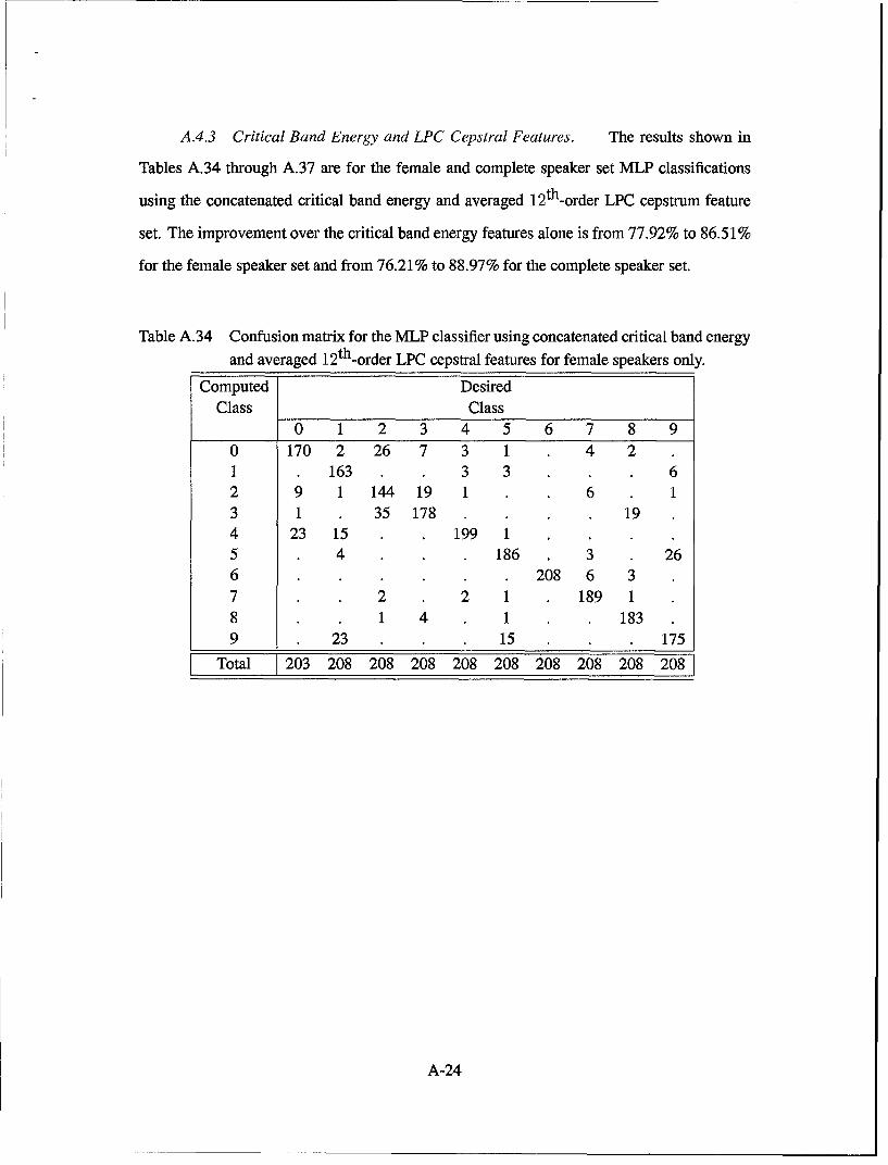
Table A.35 Overall results for the MLP classifier using concatenated critical band energyand averaged 12th-order LPC cepstral features for female speakers only.

Speaker I Classified I Errors I Accuracy (%)fl 258 31 87.98f2 259 8 96.91f3 259 28 89.19f4 259 51 80.31f5 260 19 92.69f6 260 19 92.69f7 260 25 90.38f8 260 99 61.92

Total 2075 [ 280 [ 86.51

Table A.36 Confusion matrix for the MLP classifier using concatenated critical band en-ergy and averaged 12th-order LPC cepstral features for both male and femalespeakers.


0 1 2 3 4 5 6 7 8 90 335 4 42 1 2 31 2 91 5 356 1 3 3 382 34 8 336 22 5 53 2 26 374 2 12 14 19 9 403 2 15 2 1 6 395 2 296 1 413 2 17 4 1 3 4 361 9 108 5 5 16 1 9 392 29 3 36 2 1 10 3 320

Total 410 415 415 414 414 414 414 416 416 414

A-25

Table A.37 Overall results for the MLP classifier using concatenated critical band energy andaveraged 12th-order LPC cepstral features for both male and female speakers.

Speaker Classified Errors Accuracy (%)fi 258 39 84.88f2 259 28 89.19B3 259 10 96.14f4 259 62 76.06f5 260 21 91.92f6 260 42 83.85f7 260 28 89.23f8 260 35 86.54ml 260 50 80.77m2 260 21 91.92m3 260 12 95.38m4 256 1 99.61m5 256 39 84.77m6 258 25 90.31m7 257 13 94.94m8 260 31 88.08

Total 4142 457 88.97

A-26

A.4.4 Critical Band Energy, LPC Cepstral, and LPC Coefficient Features. The

results shown in Tables A.38 through A.41 are for the female and complete speaker set MLP

classifications using the concatenated critical band energy, averaged 12th-order LPC cepstral,

and averaged 10th-order LPC coefficient feature set. The improvement over the critical band

features alone is from 77.92% to 89.07% for the female speaker set and from 76.21% to

92.40% for the complete speaker set.

Table A.38 Confusion matrix for the MLP classifier using concatenated critical band energy,

averaged 12th-order LPC cepstrum, and averaged 10th-order LPC coefficientfeatures for female speakers only.


0 1 2 3 4 5 6 7 8 90 148 17 14 1 41 3 184 2 1 52 21 6 161 2 43 29 188 11

4 26 1 203 25 3 185 1 236 2 207 1 27 1 1 2 5 198 1

8 4 1 1 1959 2 14 14 179

Total 203 208 208 208 208 208 208 208 208 208

A-27

Table A.39 Overall results for the MLP classifier using concatenated critical band energy,

averaged 12th-order LPC cepstral, and averaged 10th-order LPC coefficientfeatures for female speakers only.

Speaker Classified Errors Accuracy (%)fl 258 16 93.80f2 259 8 96.91f3 259 27 89.58f4 259 53 79.54f5 260 12 95.38f6 260 24 90.77f7 260 24 90.77f8 260 63 75.77

Total 2075 227 89.07

Table A.40 Confusion matrix for the MLP classifier using concatenated critical band energy,averaged 12th-order LPC cepstral, and averaged 10th-order LPC coefficientfeatures for both male and female speakers.


0 1 2 3 4 5 6 7 8 90 352 0 19 4 4 27 161 1 356 5 2 2 312 15 12 387 2 1 10 73 2 2 406 3 184 24 3 408 25 1 2 394 96 413 2 107 4 1 374 1 18 5 1 3879 1 42 1 1 11 350

Total 410 415 415 414 414 414 414 416 416 414

A-28

Table A.41 Overall results for the MLP classifier using concatenated critical band energy,averaged 12th-order LPC cepstral, and averaged 10th-order LPC coefficientfeatures for both male and female speakers.

Speaker Classified Errors [Accuracy (%)


Total 4142 315 92.40

A-29

Appendix B. C-shells

B.1 Introduction

This appendix contains the C-shells written to control experiments and compute results

for this work. The sections are arranged sequentially so that each experiment can be reproduced

with minimum effort. The interested reader need only pay attention to file and extension names

when reproducing the code. Questions may be directed to Capt Jeff Gay or Dr Martin DeSimio

at E-mail address [email protected] or [email protected].

Most of the routines were written to be executed within the directory containing the data.

While the shells provided in no way represent optimum code for conducting word recognition

experiments, they are proven examples. There are "man" pages available that explain the

operation of the ESPS utilities. They are obtained by typing emanfilename.

To avoid confusion, the database is broken up by individual speaker. This format is

adhered to throughout all experiments. Thus, the converted SD files are stored in directories

identified by gender and type of data (either test or training). These were further broken down

by speaker numbers ml,... , m8 for the male speaker set and fl, ... , f8 for the female speaker

set.

This format is crucial for the LNKnet experiments, since the data for each speaker

has the same filename. For example, for a 31 element feature vector belonging to any male

speaker, the filename for data stored in the directories ml, ... , m8 is m.tr31 for the training

set and m.te31 for the test set.

B.2 C-shells for Controlling ESPS Experiments

This section contains the C-shells used to manipulate data, and control the experiments

performed in this work using ESPS. Each shell was written for implementation within the

directory containing the data. In each case, a foreach loop is used to cycle through the large

number of data files.

B-1

B.2.1 Binary to Sampled Data Conversion. The following shell can be used to

convert the TI database files to ESPS FEASD, or "SD" files. This procedure is necessary

whenever the input data are given in binary form. The input files carry a .way extension, and

the output files have a .s d extension. The ESPS utility btosps performs the proper conversion

from binary to the ESPS SD format.

foreach i (*.wav)set oname = $i:rset oname = $oname.sdbtosps -f 12500 -t short -S 1024 -c "Binary to ESPS" $iend

B.2.2 Segmenting Sampled Data Files. The following shell can be used to remove

silence portions from before and after the actual utterance within a sampled speech file. This

procedure is called segmenting, and may enhance the accuracy of the classification process.

The ESPS utility that performs segmentation is called find-ep.

The input files for find-ep are the filename. sd files produced by btosps, and the output

files carry the same . sd extension. The path given for the output file location is a typical path

for this work.

foreach i (*.sd)find-ep -w $i /home/cub2/jgay/test-stuff/mtest-seg/ml/$iend

B.2.3 Converting Sampled Data Files to Acoustic Feature Files. The following

shell can be used to convert ESPS SD fies to ESPS ACF files. These "acoustic feature" files

can be used with the various classification methods provided with ESPS. The input files for

the acf utility are the filename. sd files from either btosps or find-ep, depending on whether

or not segmentation was used. The output fies carry a .acf extension.

All paths shown are particular to this work. The file acf-params is required by ESPS.

It designates the features that are to be extracted by acf. A typical acf.params file is shown

following the shell. The example below is for the male speaker set from this work.

B-2

cd Ifea..stufflfea-malelmlforeach i (*.sd)set oname = $i:rset oname = $oname.acfacf -P IParamslacf-params $i IAcousticslmjtcfsl$onameendcd Ifea-stufflfea-malelni2foreach i (*.sd)set oname = $i:rset oname = $oname.acfacf -P /Params/acf..params $i /Acoustics/m..acfs/$onameendcd Ifea-stufflfea-malelmforeach i (*.sd)set oname = $i:rset oname = $oname.acfacf -P /Params/aef-params $i IAcousticslm-acfsl$onameendcd Ifea..stufflfea-malelm4foreach i (*.sd)set oname = $i:rset oname = $oname.acfacf -P IParanislacf-params $i /Acoustics/m-acfs/$onameendcd Ifea..stufflfea..male/m5foreach i (*.sd)set oname = $i:rset oname = $oname.acfacf -P /Params/acf-params $i /Acoustics/m-acfs/$onameendcd Ifea-stufflfea-malelm6foreach i (*.sd)set oname = $i:rset oname = $oname.acfacf -P /Params/acf-params $i IAcousticslm-acfsl$onameendcd Ifea-stufflfea-malelm7foreach i (*.sd)set oname = $i:rset oname = $oname.acfad' -P /Params/acf..params $i IAcoustics/m-acfsl$onameend

B-3

cd /fea-stuff/fea-male/m8foreach i (*.sd)set oname = $i:rset oname = $oname.acfacf -P /Params/acf-params $i /Acoustics/m-acfs/$onameend

B.2.3.1 Typical acf-params File. The list shown below is a typical acf-params

file, indicating which features are to be extracted by ESPS. This particular file indicates that

pre-emphasis filtering with p = 0.95 is to be used. Also indicated are a frame length of 150

with 50% overlap using a Hamming window.

This file instructs ESPS to extract the power, zero crossing, 10th-order LPC coefficients,

12th-order LPC cepstrum, and 1024 point FFr features. Thus, with a single file, many acoustic

features are made available for classification.

string sd-field-name = "samples";float pre-emphasis = 0.950000;float frame-len = 150.000000;float start = 0.000000;float step = 75.000000;float nan = 0.000000;string window-type = "HAMMING";string units = "samples";int sdilag = 0;string sdlfname = "sd";int pwr-flag = 1;string pwrlfname = "power";int zcilag = 1;string zclfname = "zero-crossing";int aciflag = 0;string acifname = "auto-corr";int ac-order = 10;int rciflag = 0;string rclfname = "refcof";int Ipc-flag = 1;string lpclfname = "lpc.coeffs";int lartlag = 0;string larifname = "log-areaxratio";int Isfflag = 0;

B-4

string 1sf name ="line-spec-freq";float Isf-freq-res = 9.000000;jut Ipccep-flag =1;string lpccepi'name = "lpc-cepstrum";jut Ipccep-order = 12;string Ipccep-deriv = ";

float warp-param = 0.000000;jut ffcep..flag = 0;string ffcep fuame M-ffcepstrum";jut ffcep..order = 0;string ffcep-deny =

jut ff-flag = 1;jut if-order = 10;

B.2.4 Generic Header Item. In addition to the above database preparations, a

generic header item can be added to each acf file to make interpreting the classification results

easier. For this work, this was accomplished in a loop with the ESPS addgen utility, as shown

below. With the header item added, the results from a classifier such as dtw-rec are distance

measures and pairs of classes instead of distance measures and pairs of filenames

foreach i (00m*)addgen -g sequence-id -t CHAR -v zero -F $iendforeach i (01m*)addgen -g sequence-id -t CHAR -v one -F $iendforeach i (02m'*)addgen -g sequence-id -t CHAR -v two -F $iendforeach i (03m*)addgen -g sequence-id -t CHAR -v three -F $iendforeach i (04m*)addgen -g sequence-id -t CHAR -v four -F $iendforeach i (05m*)addgen -g sequence-id -t CHAR -v five -F $iendforeach i (06m*)addgen -g sequence-id -t CHAR -v six -F $i

B-5

endforeach i (07m*)addgen -g sequence-id -t CHAR -v seven -F $iendforeach i (08m*)addgen -g sequence-id -t CHAR -v eight -F $iendforeach i (09m*)addgen -g sequence-id -t CHAR -v nine -F $iend

B.2.5 Performing Dynamic Time Warping. The file below shows the commands

needed to run a complete DTW experiment for a 16 speaker data set. Again, the paths shown

are particular to this work, but represent a typical setup for this type of experiment.

To perform DTW, ESPS requires several lists. The list dtw.params tells ESPS which

acoustic features to use for classification. The following example tells ESPS to use the LPC

cepstrum for classification, and return only the closest distance measurement.

string sequence-field = "lpc-cepstrum";int delta = 0;int best-list-length = 1;

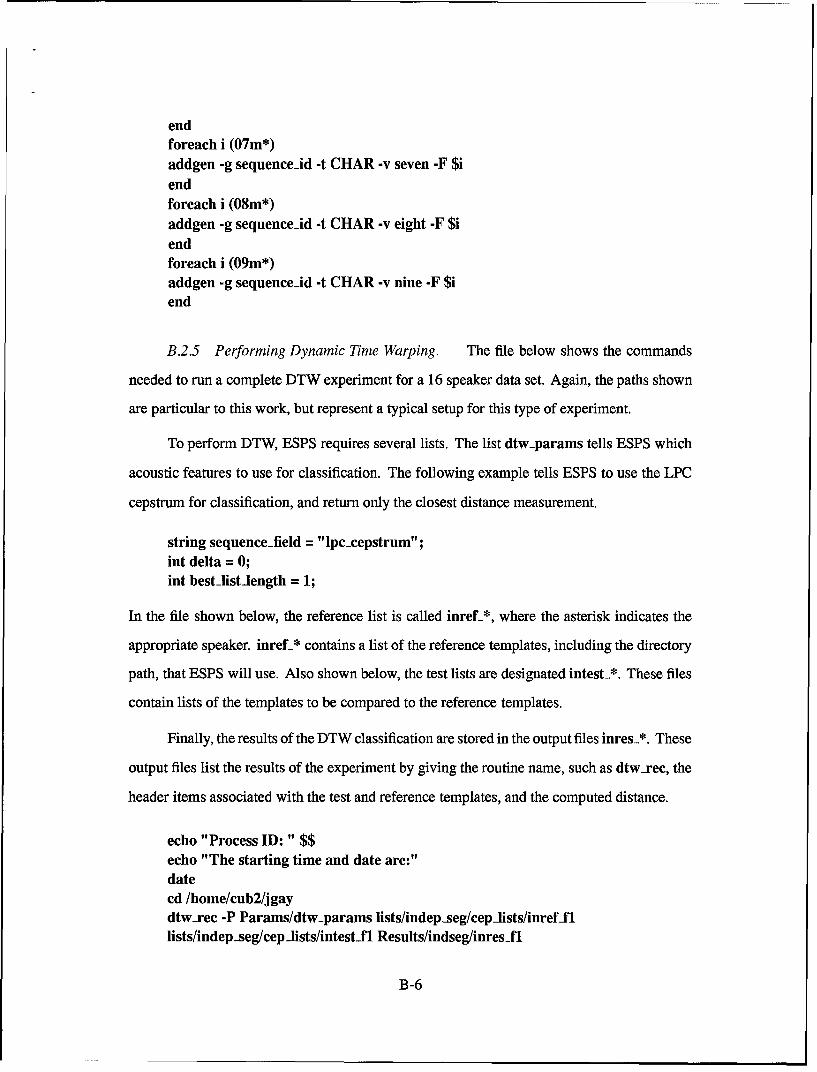
In the file shown below, the reference list is called inref_*, where the asterisk indicates the

appropriate speaker. inref_* contains a list of the reference templates, including the directory

path, that ESPS will use. Also shown below, the test lists are designated intest-*. These files

contain lists of the templates to be compared to the reference templates.

Finally, the results of the DTW classification are stored in the output files inres_*. These

output files fist the results of the experiment by giving the routine name, such as dtw-rec, the

header items associated with the test and reference templates, and the computed distance.

echo "Process ID: " $$echo "The starting time and date are:"datecd /home/cub2/j gaydtwxrec -P Params/dtw-params lists/indep-seg/ceplists/inreffllists/indep-seg/ceplists/intestfl Results/indseg/inres-fl

B-6

dtwxrec -P Params/dtw..params lists/indep-seglcep-lists/inrefl2lists/indep-seglcep-lists/intestl2 Results/indseglinresf2dtw-rec -P Params/dtw-params lists/indep..seglcep-lists/inrefi3lists/indep-seglcepiists/intestlf3 Results/indseglinresif3dtw-rec -P Params/dtw-params lists/indep-seglcep-lists/inreflf4lists/indep..seglcepiists/intest-f4 Results/indseglinresl4dtw-rec -P Params/dtw-params lists/indep..seglcepiists/inrefl35lists/indep-seglcepiists/intestlf5 Results/indseglinresi5dtw-rec -P Params/dtw-params lists/indep-seglcepiists/inref-f6lists/indep-seglcepiists/intestlf6 Results/indseglinresif6dtw-rec -P Params/dtw..params lists/indep-seglcepiists/inrefl7lists/indep-seglcep-lists/intesti'7 Results/indseglinresif7dtw-rec -P Params/dtw-params lists/indep-seglceplfists/inrefl'lists/indep..seglcep-lists/intestA'8 Results/indseg/inresl8dtw..rec -P Params/dtw-params lists/indep-seglcepiists/inref-mllists/indep-seglcepiists/intest-ml Results/indseglinres..m1dtwxrec -P Params/dtw..params lists/indep-seglcep-lists/inrefni2lists/indep-seglcepiists/intest-m2 Results/indseglinres-m2dtw-rec -P Params/dtw-params Iists/indep..seglcep-lists/inrefin3llsts/indep-seglcepiists/intestni3 Results/indseglinres-m3dtw-rec -P Params/dtw-params lists/indep-seglcep-lists/inref-m4lists/indep-seglceplists/intest-m4 Results/indseglinres-m4dtw-xec -P Paranis/dtw-params lists/indep..seglceplists/inref-m5lists/indep-seglcep-lists/intestsn5 Results/indseglinres-m5dtw-xec -P Params/dtw-params lists/indep..seg/cep-lists/inref-n6Iists/indep..seglcep-lists/intest-m6 Results/indseglinres-m6dtw-rec -P Params/dtw-params lists/indep-seglcep-lists/inref-m7lists/indep-seglcepiists/intest-m7 Results/indseglinres-m7dtwxrec -P Params/dtw..params 1ists/indep..seg/cepiists/inref-n8lists/indep-seg/cep~ists/intest-ii8 Results/indseglinres-m8echo "The stop time and date are:"date

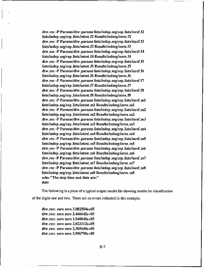
The following is a piece of a typical output results file showing results for classification

of the digits one and two. There are no errors indicated in this example.

dtw-rec: zero zero 3.082504e+05dtwxrec: zero zero 2.446642e+05dtw-rec: zero zero 1.940040e+05dtwsrec: zero zero 2.022112e+,05dtw-rec: zero zero 2.30J5640e+05dtw..xec: zero zero 3.996790e+05

B -7

dtw-rec: zero zero 2.185334e+05dtw-rec: zero zero 2.581923e+05dtw-rec: zero zero 3.141368e+05dtw-rec: zero zero 2.884247e+05dtw-rec: one one 1.918850e+05dtwirec: one one 1.772558e+05dtw-rec: one one 1.188105e+05dtw.rec: one one 1.255484e+05dtwxrec: one one 1.169767e+05dtwxrec: one one 1.287016e+05dtwxrec: one one 1.106396e+05dtw.rec: one one 1.632882e+05dtw-rec: one one 1.416697e+05dtwxrec: one one 1.187777e+05

B.2.6 Quantifying The Results From ESPS. Since the output from the procedures

discussed above are lists of raw results, a method of quantification is needed to bring it all

together. The shell listed below can be used to score the results from a DTW experiment.

awk -f iesps-utils/confawk $1

This one-line script uses awk to call the shell called confawk. Shown below, this shell

totals up the number of matches for each digit, as well as the overall number of classified

digits. These two values are used to compute a classification accuracy for each digit, which is

printed to the screen.

For this work, the shell was called results. Thus, to quantify the results of a DTW

experiment you would type results inres-ml to get the results for speaker ml. A typical output

listing is shown following the shell.

BEGIN{count = 0zeroc = 0onec = 0twoc = 0threec = 0fourc = 0fivec = 0sixc = 0

B-8

sevenc = 0eightc = 0ninec = 0rightO = 0

righti = 0right2 = 0right3 = 0right4 = 0right5 = 0right6 = 0right7 = 0right8 = 0right9 = 0}{true = $2assigned = $3if(true == "zero"){ zeroc += 1}

if(true == "one"){ onec += 1}

if(true == "two"){ twoc += 1}if(true == "three"){ threec += 1}if(true == "four"){ fourc += 1}if(true == "five"){ fivec += 1}

if(true =="six") sixc += 1}if(true == "seven"){ sevenc += 1}if(true == "eight"){ eightc += 1}

if(true == "nine"){ ninec += 1}if( true == "zero" && assigned == "zero" ) {rightO += 1}

if( true == "one" && assigned == "one" ) {rightl += 1}

if( true == "two" && assigned == "two" ) {right2 += 1}

if( true == "three" && assigned == "three" ) {right3 += 1}

if( true == "four" && assigned == "four" ) {right4 += 1}

if( true == "five" && assigned == "five" ) {right5 += 1}

if( true == "six" && assigned == "six" ) {right6 += 1}

if( true = "seven" && assigned == "seven" ) {right7 += 1}

if( true == "eight" && assigned == "eight" ) {right8 += 1}

if( true == "nine" && assigned == "nine" ) {right9 += 1}

}END{printf(" number of zeroes classified is: %d \n", zeroc)printf(" correctly classified zeros: %d \n", rightO)printf(" number of ones classified is: %d \n", onec)

B-9

printf(" correctly classified ones: %d \n", righti)printf(" number of twos classified is: %d \n", twoc)printf(" correctly classified twos: %d \n", right2)printf(" number of threes classified is: %d \n", threec)printf(" correctly classified threes: %d \n", right3)printf(" number of fours classified is: %d \n", fourc)printf(" correctly classified fours: %d \n", right4)printf(" number of fives classified is: %d \n", fivec)printf(" correctly classified fives: %d \n", right5)printf(" number of sixes classified is: %d \n", sixc)printf(" correctly classified sixes: %d \n", right6)printf(" number of sevens classified is: %d \n", sevenc)printf(" correctly classified sevens: %d \n", right7)printf(" number of eights classified is: %d \n", eightc)printf(" correctly classified eights: %d \n", right8)printf(" number of nines classified is: %d \n", ninec)printf(" correctly classified nines: %d \n", right9)printf(" zero classification accuracy: %f % \n", 100*rightO/zeroc)printf(" one classification accuracy: %f % \n", 100*rightl/onec)printf(" two classification accuracy: %f % \n", 100*right2/twoc)printf(" three classification accuracy: %f % \n", 100*right3/threec)printf(" four classification accuracy: %f % \n", 100*right4/fourc)printf(" five classification accuracy: %f % \n", 100*right5/fivec)printf(" six classification accuracy: %f % \n", 100*right6/sixc)printf(" seven classification accuracy: %f % \n", 100*right7/sevenc)printf(" eight classification accuracy: %f % \n", 100*right8/eightc)printf(" nine classification accuracy: %f % \n", 100*right9/ninec)numright = rightO + rightl + right2 + right3 + right4 + right5 + right6numright = numright + right7 + right8 + right9total = zeroc + onec + twoc + threec + fourc + fivec + sixctotal = total + sevenc + eightc + ninecoverall = numright/total

B-10

printf(" overall classification accuracy: %f \n", 100*overall)}

The following is a typical output listing created by the results C-shell listed above. The

default output device is the terminal screen, but can easily be redirected to a separate file for

each speaker.

number of zeroes classified is: 26correctly classified zeros: 26number of ones classified is: 26correctly classified ones: 25number of twos classified is: 26correctly classified twos: 25number of threes classified is: 26correctly classified threes: 24number of fours classified is: 26correctly classified fours: 26number of five classified is: 26correctly classified fives: 25number of six classified is: 26correctly classified sixes: 26number of seven classified is: 26correctly classified sevens: 26number of eights classified is: 25correctly classified eights: 25number of nines classified is: 26correctly classified nines: 24zero classification accuracy: 100.000000 %one classification accuracy: 96.153846 %two classification accuracy: 96.153846 %three classification accuracy: 92.307692 %four classification accuracy: 100.000000 %five classification accuracy: 96.153846 %six classification accuracy: 100.000000 %seven classification accuracy: 100.000000 %eight classification accuracy: 100.000000 %nine classification accuracy: 92.307692 %overall classification accuracy: 97.297297

B-11

B.2.7 Converting MATLAB Files to ESPSFEA Files. In order to perform DTW ex-

periments on features created with MATLAB, the MATLAB files must be converted to ESPSFEA

files. This can be done with the shell listed below.

foreach i (*.f9)set oname = $i:rset oname = $oname.feaaddfeahd -c "convert type" -aiesps-utils/ASCII2esps $i-/feamod/mtefea/$onameend

This script uses the ascii2esps file to format and label the MATLAB files for use with

ESPS. The typical ascii2esps file is shown below indicates that there are nine elements per

row of the input matrix. The converted data is given the label crit-band-en and designated as

floating point.

crit-band-en FLOAT 9

B.3 C-shells For Controlling LNKnet Experiments

This section lists and discusses the C-shells used to control experiments performed

using LNKnet. While LNKnet is mainly window driven, we were able to perform multiple

experiments, without accessing the windows each time, with the codes included below. This

section is designed such that if followed step by step, the interested reader should be able to

reproduce the experiments discussed in this work.

B.3.1 Preparing The Data For LNKnet. LNKnet requires ASCII data files in order

to perform its classification routines. For this work, we used either MATLAB results that were

saved in ASCII form, or the ESPS pplain utility to convert acoustic features generated with

acf to ASCII form.

LNKnet requires that the first element in each line of the ASCII data file be the class

indicator for that line. For this work, each line was a feature vector, and since we were

interested in classifying digits, the first element of each vector was one of the digits from "0"

to "9."

B-12

B.3.2 Setting The Defaults. LNKnet gets important information for classification

fromtwo defaultfiles. The files are call fname. test. default and fname. train. default.

These files tell LNKnet the number of input features to look for, the number of output classes,

the number of patterns to be tested, and the labels to attach to each pattern. An example

fname. test. default file is shown below.

describe -ninputs 31 -noutputs 10 -npatterns 260 -labelszero,one,two,three,four,five,six,seven,eight,nine

This file should be entered as a single line. The example indicates 31 features per

feature vector, ten output classes, 260 possible patterns to be classified, and that the English

words for each digits are to be attached as labels. Similarly, a fname. train, defaults file

should appear as below.

describe -ninputs 31 -noutputs 10 -npatterns 3640 -labelszero,one,two,three,four,five,six,seven,eight,nine

This file indicates 31 features per feature vector, ten output classes, and 3640 possible

training patterns, with the English words for the digits attached as labels.

The shell shown below automatically creates the proper default files for LNKnet. We

called it snb-setup. To run this file you would type snb-setup 31 1 at the command line. The

"31" indicates the number of features, and the "1" is an arbitrarily chosen speaker number.

rm indep.trainrm indep.test# enter extension to identify number of critical bandsecho begin at:dateecho Process ID is: $$foreach k ([f1[$2]/)set speaker = 'echo $k I cut -cl-2 -'

foreach i ([t1[1-8]/[fI.tr{$1} [m][1-8]/[m].tr{ $1})set j = 'echo $i I cut -cl-2 -'if ($j == $speaker) thenset pre = $i:rset namel = {$pre}.te{$1}cat $namel >> indep.test

B-13

echo $namel will hold test dataset name2 = { $pre}.tr{$1}cat $name2 > > indep.testecho $name2 will hold test dataelseset pre = $i:rset namel = {$pre}.te{$1}cat $namel >> indep.trainecho $namel copied to indep.trainset name2 = {$pre}.tr{$1}cat $name2 >> indep.trainecho $name2 copied to indep.trainendifendset ntr-pat = 'wc -1 indep.train I cut -cl-8'set nte-pat = 'wc -1 indep.test I cut -cl-8'echo $ntr-patecho $nte-patecho describe -ninputs {$1} -noutputs 10 -npatterns 3640 -labelszero,one,two,three,four,five,six,seven,eight,nine >! indep.train.defaultsecho describe -ninputs {$1} -noutputs 10 -npatterns 260 -labelszero,one,two,three,four,five,six,seven,eight,nine >! indep.test.defaultsecho finished with $speakerendecho end at:date

The first two lines of this code remove any existing . default files. Following a time

and date stamp and process ID labeling, the program cycles through the individual speaker

directories one at a time. This program is setup to perform hold-one-out speaker-independent

word recognition as described in Chapter III and in (21)

If speaker "1" is chosen when the command is entered, that speaker is "held out" of the

training process. Thus, this routine stores the patterns for speaker fl in the test .def ault s

file, and the rest of the "training" patterns in the train, defaults file.

B.3.2.1 Getting The .run File. Several files are created by LNKnet each

time an experiment is executed. In order to run multiple experiments without accessing the

windows environment, a . run file is needed. To get this, a single LNKnet experiment is

B-14

executed. Executing an experiment generates all of the necessary files for multiple passes

through LNKnet.

B.3.3 Classifying The Features With LNKnet. After obtaining the necessary files

as described above, we were able to conduct multiple experiments - one for each speaker.

This was accomplished using a shell called snb.runex. This program is nearly identical to

the setup program, except that it cycles through all sixteen speakers instead of just one. To

execute this program for a feature set containing 31 features per vector, type snb-runex 31.

The actual shell is shown below.

rm indep.trainrm indep.test# enter extension to identify number of critical bandsecho begin at:dateecho Process ID is: $$foreach k ([f][1-8]/ [m][1-8]/)set speaker = 'echo $k I cut -cl-2 -'

foreach i ([f][1-8]/[ft.tr{$1} [m][1-8]/[ml.tr{$1})set j = 'echo $i I cut -cl-2 -'if ($j == $speaker) thenset pre = $i:rset namel = {$pre}.te{$1}cat $namel >> indep.testecho $namel will hold test dataset name2 = {$pre}.tr{$1}cat $name2 > > indep.testecho $name2 will hold test dataelseset pre = $i:rset namel = {$pre}.te{$1}cat $namel > > indep.trainecho $namel copied to indep.trainset name2 = {$pre}.tr{$1}cat $name2 > > indep.trainecho $name2 copied to indep.trainendifendset ntr.pat = 'wc -1 indep.train I cut -cl-8'

B-15

set nte-pat = 'wc -1 indep.test I cut -cl-8'echo $ntr-patecho $nte-patecho describe -ninputs {$1} -noutputs 10 -npatterns 3640 -labelszero,one,two,three,four,five,six,seven,eight,nine >! indep.train.defaultsecho describe -ninputs {$1} -noutputs 10 -npatterns 260 -labelszero,one,two,three,four,five,six,seven,eight,nine >! indep.test.defaultsecho finished with $speaker# LNKnet is called here to do a train and test run for each# held out speaker Xl*.run >! results.{$speaker}rm indep.trainrm indep.testecho finished with $speakerendecho end at:date

B.3.4 Quantifying The Results. Once a set of experiments is completed, the results

need to be quantified. Notice that the classification results are saved in files designated

results f 1, ... , results .m8. These files contain confusion matrices, individual speaker

results, and a great deal of other information. In order to pick out just the individual results,

the following shell was used.

set variable sumSamp = 0set variable sumErr = 0grep model Xl*.param > total.resecho" " >> total.resecho "Results Samples Errors %Error StdDev RMS Err" >> total.resecho"-" >> total.resforeach i (results.*)grep Overall $i > > total.resset Samp = 'grep Overall $i I cut -c14-16'@ sumSamp = $sumSamp + $Sampset Err = 'grep Overall $i I cut -c25-27'@ sumErr = $sumErr + $Errendecho"-" >> total.resecho" " >> total.resawk -f /link-utils/gather total.res > > total.res

B-16

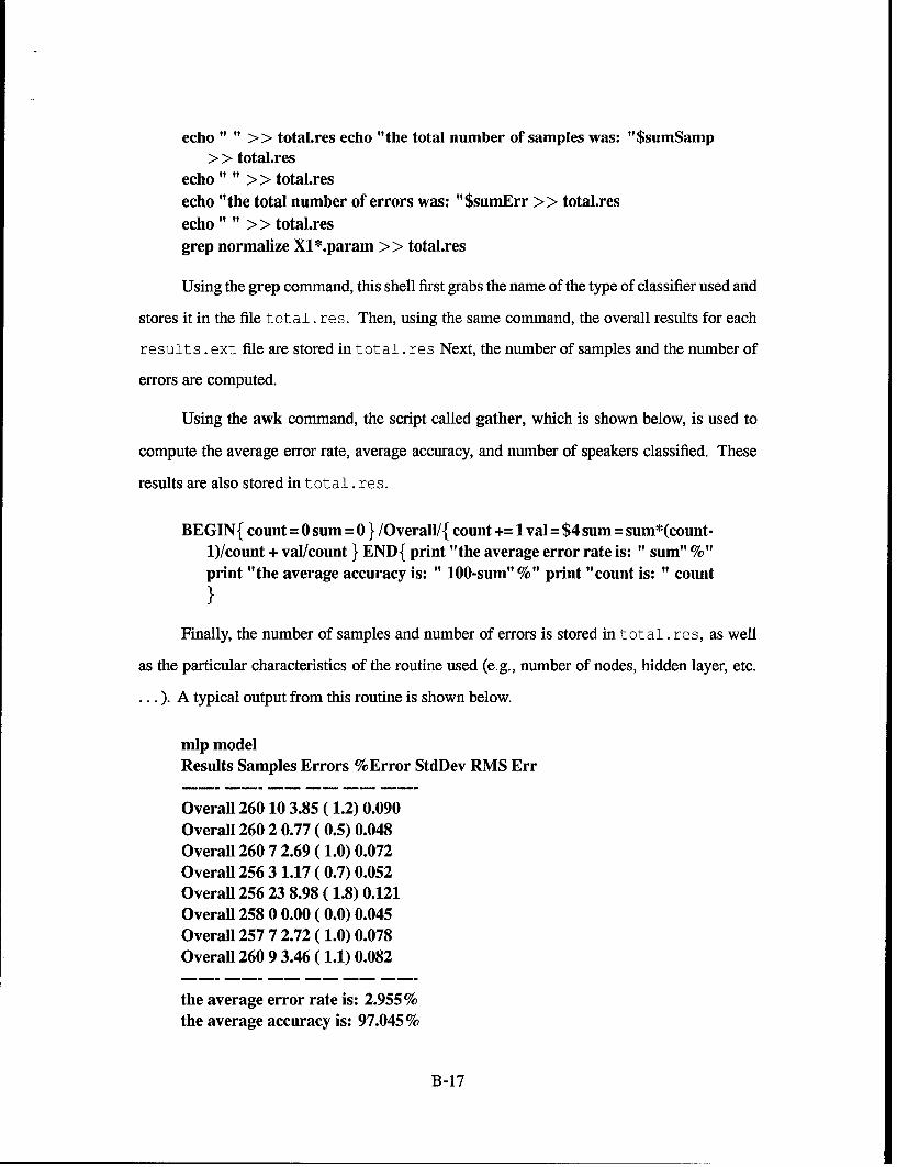
echo" " >> total.res echo "the total number of samples was: "$sumSamp> > total.res

echo" " > > total.resecho "the total number of errors was: "$sumErr >> total.resecho" " >> total.resgrep normalize X1*.param > > total.res

Using the grep command, this shell first grabs the name of the type of classifier used and

stores it in the file total. res. Then, using the same command, the overall results for each

results. ext file are stored in total. res Next, the number of samples and the number of

errors are computed.

Using the awk command, the script called gather, which is shown below, is used to

compute the average error rate, average accuracy, and number of speakers classified. These

results are also stored in total. res.

BEGIN{ count = 0 sum = 0 } /Overall/{ count += 1 val = $4 sum = sum*(count-1)/count + val/count } END{ print "the average error rate is: " sum" %"print "the average accuracy is: " 100-sum" %" print "count is: " count

}Finally, the number of samples and number of errors is stored in total. res, as well

as the particular characteristics of the routine used (e.g., number of nodes, hidden layer, etc.

... ). A typical output from this routine is shown below.

mip modelResults Samples Errors %Error StdDev RMS Err

Overall 260 10 3.85 ( 1.2) 0.090Overall 260 2 0.77 (0.5) 0.048Overall 260 7 2.69 (1.0) 0.072Overall 256 3 1.17 (0.7) 0.052Overall 256 23 8.98 ( 1.8) 0.121Overall 258 0 0.00 (0.0) 0.045Overall 257 7 2.72 (1.0) 0.078Overall 260 9 3.46 (1.1) 0.082

the average error rate is: 2.955%the average accuracy is: 97.045%

B-17

count is: 8the total number of samples was: 2067the total number of errors was: 61-debug 0 -verbose 3 -verror I -nodes 31,25,10 -alpha 0.6 -etta 0.1

B.3.4.1 Extra Procedures For MLP Quantification. If the classifier used was

a MLP, there is an extra step necessary to obtain the quantified results of the experiments.

Before running the routine described above, the shell shown below must be executed. This

shell arranges the results for use with the above routine, and stores them in the files mip re s . f 1,

.... mlpres.m8.

foreach i (results.*)set name = $i:esed -n '138,156 p' $i >! mlpres.$nameend

Once this is completed, the original quantifying script should be altered such that

results. * is replaced by mipres. * in the loop argument. Also, the word "normalize"

should be replaced with "nodes." It is helpful to have separate shells instead of continuously

altering the original shell.

B.3.5 Obtaining an Overall Confusion Matrix. To get an overall confusion matrix

for the MLP classifier from the individual matrices provided for each speaker, the shell shown

below can be used.

mlp-confuscoldcut grpmatrefuz prepmatcleanup

This script calls four separate shells that each perform a specific task. The shell called

mlp.confus, shown below, cuts the confusion matrices out of each individual results . * file

and stores them in the file called grpmat.

foreach i (results.*)set name = $i:e

B-18

sed -n '123,132 p' $i >> grpmatend

Next, the script called coldcut, shown below, uses a different script called blank2zero

to place the digit "0" into the blank spaces in the original confusion matrices.

cut -c4 $1 >! bob-linescut -clO-12 $1 >! bob-zeroescut -c16-18 $1 >! bob-onescut -c22-24 $1 >! bobtwoscut -c28-30 $1 >! bob-threescut -c34-36 $1 >! bob-fours

cut -c40-42 $1 >! bob-fivescut -c46-48 $1 >! bob-sixescut -c52-54 $1 >! bob-sevenscut -c58-60 $1 >! bob-eightscut -c64-66 $1 >! bob-ninescut -c71-73 $1 >! bob-totalsawk -f Ilink-utils/blank2zero bob-lines >! reallinesawk -f /link-utils/blank2zero bob-zeroes >! real-zeroesawk -f /link-utils/blank2zero bob-ones >! real-onesawk -f /link-utils/blank2zero bobtwos >! real-twosawk -f /link-utils/blank2zero bob-threes >! real-threesawk -f /link-utils/blank2zero bob-fours >! real-foursawk -f /link-utils/blank2zero bob-fives >! real-fivesawk -f /link-utils/blank2zero bob-sixes >! real-sixesawk -f /link-utils/blank2zero bob-sevens >! real-sevensawk -f /link-utils/blank2zero bob-eights >! real-eightsawk -f /link-utils/blank2zero bob-nines >! real-ninesawk -f /link-utils/blank2zero bob-totals >! real-totals

paste real-lines real-zeroes real-ones real-twos real-threes real-foursreal-fives real-sixes real-sevens real-eights real-ninesreal-totals >! prepmat

The results from this script are stored in a file called prepmat. The blank2zero script

is shown below.

{ printf(" %d \n" ,$1) }

Finally, the shell called refuz constructs the overall confusion matrix using yet another

shell called fuzme. These two files are shown below in order of precedence.

B-19

awk -f-/link-utils/fuzme $1 > total.con

BEGIN{ count = 0total = 0zeroc = 0 onec = 0twoc = 0threec = 0fourc = 0fivec = 0sixc = 0sevenc = 0eightc = 0ninec = 0zero-one = 0zerotwo = 0zerothree = 0zero-four = 0zero-five = 0zero-six = 0zero-seven = 0zero-eight = 0zero-nine = 0zero-total = 0one-zero = 0one-two = 0onethree = 0one-four = 0one-five = 0one-six = 0one-seven =0one-eight = 0one-nine = 0one-total = 0two-zero = 0two-one = 0two-three = 0two-four = 0two-five = 0two-six = 0two-seven = 0two-eight = 0two-nine = 0two-total = 0

B-20

three-zero = 0three-one = 0three-two = 0three-four =0three-five = 0three-six = 0three-seven = 0three-eight = 0three-nine = 0three-total = 0four-zero = 0four-one = 0four-two = 0four-three = 0four-five = 0four-six = 0four-seven = 0four-eight = 0four-nine = 0four-total = 0five-zero = 0

five-one = 0five-two = 0

five-three = 0five-four = 0five-six = 0

five-seven = 0five-eight = 0five-nine = 0five-total = 0

six-zero = 0six-one = 0six-two = 0six-three = 0six-four = 0six-five = 0

six-seven = 0six-eight = 0six-nine = 0six-total = 0seven-zero = 0seven-one = 0

B-21

seven-two = 0seven-three = 0seven-four = 0seven-five 0

seven-six = 0seven-eight = 0seven-nine = 0seven-total = 0eight-zero 0eight-one = 0eight-two - 0eight-three = 0eight-four = 0

eight-five = 0eight-six = 0eight-seven = 0eight-nine = 0eighttotal = 0nine-zero 0

nine-one = 0nine-two = 0nine-three = 0nine-four = 0nine-five = 0nine-six = 0nine-seven = 0nine-eight = 0

nine-total = 0}{linenum = $1addO = $2addi = $3add2 = $4add3 = $5add4 = $6add5 = $7add6 = $8add7 = $9add8 = $10add9 = $11addtot = $12

B-22

if(linenum == "O"){zeroc = zeroc + addOzero-one = zero-one + add1

zerotwo = zerotwo + add2

zero-three = zero-three + add3

zero-four = zero-four + add4zero-five = zero-five + add5

zero-six = zero-six + add6zero-seven = zero-seven + add7zero-eight = zero-eight + add8zero-nine = zero-nine + add9zerototal = zerototal + addtot}if(linenum == "l"){onec = onec + addlone-zero = one-zero + addOone-two = one-two + add2onethree = one-three + add3one-four = one-four + add4one-five = one-five + add5one-six = one-six + add6one-seven = one-seven + add7one-eight = one-eight + add8one-nine = one-nine + add9one-total = onetotal + addtot}if(linenum == "2"){twoc = twoc + add2two-zero = two-zero + addOtwo-one = two-one + add1two-three = twothree + add3two-four = two-four + add4two-five = two-five + add5two-six = two-six + add6two-seven = two-seven + add7two-eight = two-eight + add8two-nine = two-nine + add9two-total = twototal + addtot}if(linenum == "3"){threec = threec + add3

three-zero = three-zero + addOthree-one = three-one + add1three-two = threetwo + add2three-four = three-four + add4three-five = three-five + add5three-six = three-six + add6three-seven = three-seven + add7three-eight = three-eight + add8

B-23

three-nine = three-nine + add9three-total = three-total +i addtot}if(linenum == "4"){fourc = fourc + add4f'our-zero =four-zero + addOfour-one =four-one + addl.four-two =four-two + add2four-three = four-three + add3four-five = four-five + add5four-six = four-six + add6four-seven =four-seven + add7four-eight =four-eight + add8four-nine = four-nine + add9four-total = four-total + addtot}if(linenum == "5"){flvec = flvec + add5five-zero = flve-zero + addOfive-one = five-one + addifiveiwo = fiveiwo + add2flveihree = flve-three + add3five-four = five-four + add4five-six = five-six + add6five-seven =five-seven + add7five-eight =five-eight + add8five-nine = five-nine + add9flve-total = five-total + addtot}if(linenum == "6")f{sixc = sixc + add6six-zero = six-zero + addOsix-one = six-one + addisix-two = sixitwo + add2sixihree = sixihree + add3six-four = six-four + add4six-five = six-ilve + add5six-seven =six-seven + add7six-eight =six-eight + add8six-nine = sixunine + add9sixitotal = sixitotal + addtot}if(linenum == "7"){sevenc = sevenc + add7seven-zero =seven-zero + addOseven-one =seven-one + addisevenitwo =sevenitwo + add2seven-three = seven-three + add3seven-four = seven-four + add4seven-five = seven-five + add5

B -24

seven-six = seven-six + add6seven-eight =seven-eight + add8seven-nine =seven-nine + add9seveniotal =seven-total + addtot}if(linenum == "8"){eighte eightc + add8eight-zero =eight-zero + addOeight-one =eight-one + addieigh~two =eigh~two + add2eigh~three = eight-three + add3eight-four = eight-four + add4eight-five = eight-five + add5eight-six = eight-six + add6eight-seven =eight-seven + add7eight-nine = eight-nine + add9eigh~total = eigh~total + addtot}if(linenum == "9"){ninec ninec + add9nine-zero nine-zero + addOnine-.one =nine-one + addinine-two =nineiwo + add2nineihree = nineihree + add3nine-four = nine-four + add4nine-five = nine-five + add5nine-six = nine-six + add6nine-seven =nine-seven + add7nine-eight =nine.-eight + add8nine total =nineiotal + addtot}

END{ printf(" %d %d %d %d %d %d %d %d %d %d %d\ n", zeroc,zero-one,zero-two,zero three zero. four,zero-five,zero-six,zero-seven,zero-eight,zero.-ine,zero-tota1)printf(" %d %d %d %d %d %d %d %d %d %d %d\ n", one-zero,onec,one-two,oneihree one-four,one-five,one-six,one-seven,one..eight,one-nine,one-total)printf(" %d %d %d %d %d %d %d %d %d %d %d\ n", two-zero,two-one,twoc,two~hree,two-four,two-five,two-six,two-seven,two-eight,two-nine,two-total)printf(" %d %d %d %d %d %d %d %d %d %d %d\ n", three-zero,three-one,three-two,threec,threei'our,three-ive,three-six,three-seven three-eight,three-nine,three-total)printf(" %d %d %d %d %d %d %d %d %d %d %d\ n", four-zero,four-one,four..two,fourihree,fourc,four-five,four-six,four-seven,four-eight,four-nine,four-total)

B -25

printf(" %d %d %d %d %d %d %d %d %d %d %d\n", five-zero,five-one,fivetwo,fivethree,five-four,fivec,five-six,five-seven,five-eight,five-nine,five-total)

printf(" %d %d %d %d %d %d %d %d %d %d %d\n", six-zero,six-one,sixtwo,sixthree,sixifour,

six-five,sixc,six-seven,six-eight,six-nine,sixAotal)printf(" %d %d %d %d %d %d %d %d %d %d %d\n", seven-zero,seven-one,seven-two,seventhree,sevenfour,seven-five,s,seven-six,sevenc,seven-eight,seven-nine,seven-total)printf(" %d %d %d %d %d %d %d %d %d %d %d\n", eight-zero,eight-one,eighttwo,eightthree,eight-four,eight-flve,eight-six,eight-seven,eightc,eight-nine,eight-total)printf(" %d %d %d %d %d %d %d %d %d %d %d\n", nine-zero,nine-one,nine-two,ninethree, nine-four,nine-five,nine-six,nine-seven,nine-eight,ninec,nine-total)}

The first thing this file does is initialize a multitude of variables. Next, the fields in

prepmat that contain the class and each of the digits are stored in the variables linenum, addO,

add9, and addtot. This is followed by a count of each digit for each line in prepmat.

Next, the lines containing the totals for each digit are printed to the file total. con.

Finally, the cleanup removes from the current directory the multitude of files that are created

by this process. Thus, the overall confusion matrix is stored in total . con.

B.3.5.1 Modifications For Other Classifiers. If a classifier other than the

MLP is used, the routine mlp-confus will probably have to be modified for the overall

confusion matrix procedure to work properly, since the individual confusion matrices are

located at different line numbers in the result s .ext file based on which classifier was used.

The only modification necessary is in the "sed" line of this routine. In this line, substitute

the appropriate line numbers for "123,132." It is helpful to have separate files to quantify the

results of different classifiers.

B-26

B.4 Feature Vector Averaging

The following program, written in C, was provided by Captain Dave Jennings. This

program is used to compute the average LPC coefficient and LPC cepstral coefficient features

for the acoustic features converted from the ESPS ACF format to ASCII. The program requires

lists designating the input file names and the class that the file falls in as shown in the example

below.

00mlsetO.acf 001mlsetO.acf 102mlsetO.acf 2

09mlsetO.acf 9

It should be noted that there is a bug in this program. The output is typically a file of

vectors of all utterances of the ten digits by a single speaker, with the class attached as the first

element of each vector. For some reason, the code duplicates the last vector. For this work,

the last vector is simply deleted from each file.

After compiling the code, the feature vectors are averaged by calling the routine as

follows.

lpcmeans listname /path/outfile.ext

The actual program is shown below. The variable numlpc can be set to accommodate

any number of coefficients.

Program Name: LPCmeans.cThesis Task : Neural nets on features on isolated word recognition.Program Task : Calculate the means of the lpc-cepstral data and outputthe information in a format compatible with LNKnet.Author: Lt David L. JenningsWritten: 4 Aug 1994

/* ................... MAIN PROGRAM ......................... *main(int argc,char *argvyl){

B-27

FILE *jn-file,*out-fjle,*file-ljst;jut count,i,numlpc;char fname[80],class[80];float a[20],mean[1201;* ..... Check command line arguments......

if(argc<2)

printf(" You need to provide the names of input and outputfiles.\nV1);printf("The format is: LPCmeans {input file list} {outputfile}\n");exit(1);

1*........... Open input files..............if((file-iist =fopen(argv [1]," r" ))= =NULL)

printf(" Cannot open input file\ n")

exit(1);

Iif((outiile =fopen(argv[121," w" ))==NULL)

Iprintf("Cannot open output file\n");exit(1);

Inumlpc = 12;while(!feof(file-list))

Ifscanf(file-list," %s" ,fname);fscanf(fileilist," %s" ,class);if((in-file = fopen(fname," r" ))==NULL)

Iprintf(" Cannot open input file specified in file list.\n");printf(" %s is the culprit" ,fname);exit(1);

Ifor (i=0;i<numlpc;i++) mean[i] = 0;count = 0;for (i=0;i<numlpc;i++) fscanf(in-file," %f" ,&a[i]);while(!feoffin-file))

Ifor (i=0;i<numlpc;i++) mean[i] = mean[i] + a[i];for (i=0;i<numlpc;i++) fscanf(in-.file," %f" ,&a[i]);

B-28

count+i+;

for (i=O;i<numlpc;i++) mean[i] = mean[iI/count;for (i=O;i<numlpc;i-i+) printf(" %5.4f ",meanfi]);printfC' \n" );felose(in-file);fprintf(outfile," %s ",class);for (i=O;i<numlpc;i-i+) fprintf(out-file," %5.4f ",mean[i]);fprintf(out-file," \')Ifelose(fileilist);felose(out-file);

B -29

Appendix C. MATLAB Files

C.1 Introduction

This appendix contains the m-files and functions used for this work. In many cases,

multiple files exist that perform the same functions, but for different speaker sets. This is

noted in the descriptions that accompany each file, but only one example of each file is given.

C.2 Critical Band Energy Feature Calculation for the Training Data Set

The following m-file can be used to compute the critical band energy features from a

set of binary sampled data speech files. This file was used to create feature vectors for the

male training set from the TI data base. Another file was created to compute the features for

the female training set.

%function []=mtrainfeat(window,overlap)clear

% Masters Thesis"% Advisor: Dr Martin P. DeSimio, [email protected]"% Student: Capt Jeffrey M. Gay, [email protected]"% Program: mtrainfeat.m

"% PURPOSE: Spectrogram and feature vector computation."% DESCRIPTION: This m-file compute critical band energy features for"% each input file. First, a spectrogram is computed for the"% file, then the features vectors are created from the"% spectrograms. The results are stored in matrices comprised"% of the set of all utterances of the same digit for each"% speaker. That is, each matrix contains the features"% representing all utterances of the same digit for a"% particular speaker. The data are saved in ascii form.

% BEGIN:

% 1. Set frame length to 150 samples.% 2. Set frame overlap to 50%.% 3. Determine number of frame shifts to be completed.

C-1

window = 150;overlap = 1/2;

OL = fix(window*(1-overlap));

% 1. Read the data.

forj 1:8;for k =0:9for i= 0:9filename = ['O',int2str(k),'m',int2str(j),'set',int2str(i)];fname = [filename,'.wav'];fid = fopen(fname,'r');data = fread(fid,'short');fclose(fid);data = data(513:length(data));

% 1. Remove one frame length from the data length.% 2. Determine number of windows needed.

N = length(data);done = fix((N-window)/OL);

% Compute spectrogram-

% 1. Multiply frame by given window.% a. Rectangular implied if no "win" selected.% 2. Compute Fourier transform, and select zero to pi points.

% 3. Average the frequency bin over time.

windat = zeros(window,1);win = hamming(window);for ii= 1:donestop = window + (OL*ii-OL);start = 1 + (OL*ii-OL);temp - data(start: stop);windat(:,ii) = win .* temp;endWindat = abs(fft(windat,256));Windat = Windat((1:128),:);[m,n] =size(Windat);

timeavg(i+l,:) = (1/n)*sum(Windat');Windat = -Windat;

C-2

end

% 1. Set counter for number of features per vector.

for b = 6:3:24

% 1. Compute bin endpoint locations based on critical band scale.

delta = 128/6250;end-pt(1) = 380;piece = (2000 - 380) / b;for s = 2:bend-pt(s) = end-pt(s - 1) + piece;endend-pt(b + 1) = 2000;Lh = (exp(end-pt*log(2)/1000) - 1)*1000;bin-temp = round(fLh * delta);right = [bin-temp(2:b) - 1,bin-temp(b + 1)];

bins = [bin-temp(l :b)',right'];

% 1. Average the critical band frequency windows.

for y = 1:10for kk = l:bforl= 1:2a(l) = bins(kk,l);endcount = a(1):a(2);div = length(count);freqavg(y,kk) = (1/div)*sum(timeavg(y,a(1):a(2)));endend

% 1. Store the matrix containing the critical band energy features.

filename2 = ['m',int2str(j),'dig',int2str(k),'all'];fname = [filename2,'.f',int2str(b)];savmag = ['save ',fname,' freqavg -ascii'];eval(savmag);clear end-ptclear freqavgend

C-3

clear timeavgendend

C.3 Critical Band Energy Feature Calculation for the Testing Data Set

The following m-file can be used to compute the critical band energy features from a

set of binary sampled data speech files. This file was used to create feature vectors for the

male test set from the TI data base. Another file was created to compute the features for the

female test set.

%function[]=mtrainfeat(window,overlap)clear

"% Masters Thesis"% Advisor: Dr Martin P. DeSimio, [email protected]"% Student: Capt Jeffrey M. Gay, [email protected]"% Program: mtestfeat.m

"% PURPOSE: Spectrogram and feature vector computation."% DESCRIPTION: This m-file compute critical band energy features for"% each input file. First, a spectrogram is computed for the"% file, then the features vectors are created from the"% spectrograms. The results are stored in matrices comprised"% of the set of all utterances of the same digit for each"% speaker. That is, each matrix contains the features"% representing all utterances of the same digit for a"% particular speaker. The data are saved in ascii form.

% BEGIN:

% 1. Set frame length to 150 samples.% 2. Set frame overlap to 50%.% 3. Determine number of frame shifts to be completed.

window - 150;overlap - 1/2;OL = fix(window*(1-overlap));

% 1. Read the data.

C-4

forj = 1:8;for k = 0:9for m = 0:1fori= 1:8filename = ['O',int2str(k),'m',int2str(j),'s',int2str(i),'t',int2str(m)];fname = [filename,'.wav'];fid = fopen(fname,'r');if fid == -1Warning = ['The data 0',int2str(k),'m',int2str(j),'s',int2str(i),'t',...int2str(m),' is missing or inaccessible.']elsedata = fread(fid,'short');fclose(fid);data = data(513:length(data));

% 1. Remove one frame length from the data length.% 2. Determine number of windows needed.

N = length(data);done = fix((N-window)/OL);

% Compute spectrogram-% 1. Multiply frame by given window.% a. Rectangular implied if no "win" selected.% 2. Compute Fourier transform, and select zero to pi points.% 3. Sum the frequency bin over time.

windat = zeros(window, 1);win = hamming(window);for ii = 1:donestop = window + (OL*ii-OL);start = 1 + (OL*ii-OL);temp = data(start: stop);windat(:,ii) = win .* temp;endWindat = abs(fft(windat,256));Windat = Windat((1:128),:);[zz,n] =size(Windat);timeavg(i+m*8,:) = (1/n)*sum(Windat');Windat = -Windat;clear data

C-5

endendend

% 1. Set counter for number of features per vector.%

for b = 6:3:24

% 1. Compute bin endpoint locations based on critical band scale.

delta = 128/6250;end-pt(1) = 380;piece = (2000 - 380) / b;for s = 2:bend-pt(s) = end-pt(s - 1) + piece;endend-pt(b + 1) = 2000;fh = (exp(end-pt*log(2)/1000) - 1)* 1000;bin-temp = round(fih * delta);right = [bin-temp(2:b) - l,bin-temp(b + 1)];

bins = [bin-temp(l:b)',right'];

% 1. Average the critical band frequency windows.

for y = 1:16for kk = 1:bfor I = 1:2a(l) = bins(kk,l);endcount = a(1):a(2);div = length(count);freqavg(y,kk) = (1/div)*sum(timeavg(y,a(l):a(2)));endend

% 1. Store the matrix containing the critical band energy features.

filename2 = ['tin',int2str(j),'dig',int2str(k),'all'];fname = [filename2,'.f',int2str(b)];savmag = ['save ',fname,' freqavg -ascii'];eval(savmag);clear end-pt

C-6

clear freqavgendclear timeavgendend

C.4 Adding The Class Indicator To The Feature Vectors

Before the features created from the previous file can be used with LNKnet, a class

indicator must be added as the first element of each feature vector. This could be incorporated

into the previous file, but for this work, was left to the file shown below.

This file adds a non-integer class as the first element of each feature vector. This happens

because the rest of the data in each vector is floating point data. If integer class indicators are

desired, conversion is most easily done with the vi editor.

clear

% Masters Thesis% Advisor: Dr Martin P. DeSimio, [email protected]% Student: Capt Jeffrey M. Gay, [email protected]% Program: addclass.m

% PURPOSE: Add a class indicator as the first element of each% feature vector.% DESCRIPTION: This program adds as the first element of each% feature vector a class indicator. For the digits, this is% one of the numbers 0, ... , 9. The files, which are% matrices of features, are then stacked and stored according% to speaker sex and number.

% BEGIN:

% 1. Set variable equal to feature vector length.% 2. Initialize counters.% 3. Load feature files% 4. Concatenate class and feature vectors.% 5. Increment counters.% 6. Stack the features.% 7. Save the new feature files.

C-7

z = 9;for j =8:8cntmI = 0;cntm2 = 0;cntf 1 = 0;cntf2 = 0;for k =0:9classm = fix((zeros(1, 10) + k)');classf = fix((zeros(1, 10) + k)');ifilenamel = ['in',int2stroj), 'dig' ,int2str(k), 'all'];fflename2 = ['f' ,int2stroj), 'dig' ,int2str(k), 'all'];fnamel = [filenamel ,'.f',int2str(z)];fname,2 = [filename2, '.f',int2str(z)];fnamel = [filenamel,'.asc'];fname2 = [filename2,'.asc'];eval(['load 'fnamel]);eval(['load 'fname2]);eval(['m ',int2stroj), 'dig' ,int2str(k), 'all[classm~m' ,int2stroj), 'dig' ,int2str(k), 'all];'])eval(['f',int2stroj),'dig',int2str(k),'alI =[classf,f' ,int2stroj), 'dig' ,int2str(k). 'all];'])cntml = 10*k + 1;cntmn2 = crtntmI + 9;cntfl = 10O*k + 1;cntf2 = cntf 1 + 9;eval(['tempm((cntml1:cntm2),:) = in',int2stroj), 'dig' ,int2str(k), 'all;'])eval(['clear ','m' ,int2stroj), 'dig' ,int2str(k), 'all;'])eval(['teinpf((cntfl1:cntf2),:) = f' ,int2stroj), 'dig' ,int2str(k), 'all;'])eval(II'clear ','f ',int2stroj), 'dig' ,int2str(k), 'all;'])end[roa,coa] = size(tempin);savenamelur = ['mtrainspkr ',int2strOj)];

snarnelin = [savenameim. ' .L',int2str(coa - 1)];eval(['save ',snamelmi,' teinpi -ascii ']);savenameif = ['ftrainspkr ',int2strOj)];

snameif = [savenamel1f, '.L',int2str(coa - 1)];eval(['save ',snamelf,' tempf -ascii']);end

% 1. Initialize counters.% 2. Load feature files.

C-8

% 3. Concatenate class and feature vectors.% 4. Increment counters.% 5. Stack the features.% 6. Save the new feature files.

for j =8:8jm = 0;

jf = 0;cntml = 0;cntm2 = 0;cntf 1 = 0;cntf2 = 0;for k =0:9classtmn = fix((zeros(1,16) + k)');classtf = fix((zeros(1,16) + k)');filenamel = ['tin',int2stroj), 'dig' ,int2str(k), 'all'];filename,2 = ['if' ,int2stroj), 'dig' ,int2str(k), 'all'];fnamel = [filename 1,' .f' ,int2str(z)];fname2 = [filename2, '.f ',int2str(z)];

fnamel = [filenamel,'.asc'];fname2 = [filename2,'.asc'];eval(['load 'fnamel]);eval(['load 'fname2]);eval(II'tm' ,int2stroj), 'dig' ,int2str(k), 'all[classtm,tm' ,int2stroj), 'dig' ,int2str(k), 'all];'])eval(['tf ',int2stroj).'dig' ,int2str(k), 'all =

[classtf,tf ',int2stroj), 'dig' ,int2str(k), 'all];'])cntml = 16*k + 1;cntm2 = cntml + 15;cntfl = 16*k + 1;cntf2 = cntfl + 15;eval(['temptm((cntmnl:cntm2),:) = tn' ,int2stroj), 'dig' ,int2str(k), 'all;'])eval(['clear ','tm' ,int2stroj), 'dig' ,int2str(k), 'all;'])eval(['temptf((cntf 1 :cntf2),:) = tf' ,int2stroj), 'dig' ,int2str(k), 'all;'])eval(['clear ','if' ,int2stroj), 'dig' ,int2str(k), 'all;'])end[rob,cob] = size(temptm);savename2m = ['mtestspkr ',int2stroj)];

sname2m =[savename2m,'.L',int2str(cob - 1)];

eval(['save ',sname2m,' temptin -ascii']);savename2f = ['ftests~pkr' ,int2strOj)];sname2f = [savename2f,'.L',int2str(cob - 1)];

C-9

eval(['save ',sname2f,' temptf -ascii']);end

C.5 Energy Window Computation

The following m-file computes the energy in each of nine identical length segments

of each digit utterance. Each "energy profile" result is a feature in an energy profile feature

vector.

clear

% Masters Thesis% Advisor: Dr Martin P. DeSimio, [email protected]% Student: Capt Jeffrey M. Gay, [email protected]% Program: profile.m

"% PURPOSE: Compute the energy in nine separated equal sized segments"% spanning each input speech sample."% DESCRIPTION: This program detects the endpoints of an input speech"% sample by first computing the envelope of the data, then"% thresholding the envelope. The endpoints are those points"% at which the threshold is initially and finally breached."% Using this "segmented" data, an energy profile is computed"% for a selected number of energy windows. The Energy is% normalized to 1.

% BEGIN:

% 1. Read a data file.% 2. Normalize the amplitude of the sample for a maximum value of 1.% 3. Compute the envelope of the sample data.

for j =8:8for k =0:9for i= 0:9filename = ['0',int2str(k),'m',int2str(j),'set',int2str(i)];fname = [filename,'.wav'];fid = fopen(fname,'r');data = fread(fid,'short');fclose(fid);data = data(513:length(data));

C-10

norm-div = max(abs(data));norm-dat = data / norm-div;check = abs(norm-dat);[b,a] = butter(5,0.008);Y = filter(b,a,check);Y-norm-div =max(Y);

Y-norm = Y /Y-.norm-div;

% 1. Find the endpoints based on empirically derived threshold.

done = length (Y-.norm);cnt = 0;for s= L~doneif Y-.norm(s) >= 0.0063 15cnt =cnt + 1;stop..pt s ;if cnt == 1start-pt s ;endendend

% 1. Segment the data based on the computed endpoints.% 2. Compute the normalized energy for each segment.% 3. Store results in ascii form.

seg-dat = data(start-pt:stop-pt);E = seg-dat' * seg-dat;norm..E = seg-dat / sqrt(E);[ro,col] = size(seg-dat);increase = floor(ro/9);for s = 1:9inda = 1 + (s - 1) * increase;indb, = increase * s;chunk(:,s) = norm-E(inda:indb,1);endbob-E(i+1,:) = sum(chunk. ^2);clear chunkendfiename2 = ['in',int2stroj), 'dig',int2str(k), 'all'];fname2 = [filename2,'.asc'];eval(['save ',fname2,' bob-E -ascii'])

C-11

endend

C.6 Concatenating Feature Vectors

The following m-file may be used to concatenate feature vectors. Again, this example

covers the male feature set, but is easily modified for the female feature set. Be sure to remove

the class indicator from the feature vectors being attached, or you will have a class indicator

in the middle of your new feature vectors. A file to remove the indicator is given in the next

section.

clear

"% Masters Thesis"% Advisor: Dr Martin P. DeSimio, [email protected]"% Student: Capt Jeffrey M. Gay, [email protected]% Program: concat.m

"% PURPOSE: Concatenate different feature vectors to be used"% later in recognition experiments.% DESCRIPTION: This program concatenates two input vectors to create"% a single feature vector. Concatenation is by class, but"% only one first input vector should have the class included"% as the first elements of each vector. If needed, the file"% "bobcat.m" can be used to remove the classes from the"% second input vector before use in this file.

% FORMAT:

% 1. The naming convention for files containing the classes is% m.tr21 for a 21-element feature vector, from the training% set.% 2. The naming convention for classless files is mlcat.tr21 for% speaker ml, 21-element feature vectors, from the training% set.

% BEGIN:

% 1. Load vectors to be concatenated.% 2. Concatenate vectors.

C-12

% 3. Store new vectors in ascii form.

for j=1:8ifienamel = ['m',int2stroj)];fflename3 = ['m',int2str0j),'cat'iI;filename4 = ['tm',int2str0j),'cat'];filename5 = ['treat' ,int2stroj)];fflename6 = ['tecat',int2stroj)];fhamel = [filenamel,'.tr2l'];fname2 =[filenamel,'.te2l '];fname3 = [filename3,'.asc'];fhame4 = [filenamne4, '.asc'];fname5 = [filename5,'.tr2l'];fhame6 = [filename6,'.te2l '];eval(['load 'fnamel1]);eval(['load 'fname3]);eval([II'oad 'fname4]);eval(II'traincatn' ,int2str0j),' = [in',int2stroj), ',m' ,int2stroj), 'cat]; 'i)eval(['save ',fname5,' traincatm' ,int2stroj),' -ascii'])eval(II'clear m' ,int2stroj)])eval([II'oad ', fname2]);eval(['testcatm'jnt2str0j),' = [m' ,int2stroj), ',tm' ,int2stroj), 'cat];'])eval(II'save ',fname6,' testcatm' ,int2stroj),' -ascii'])end

C.6.1 Removing The Classes From A Feature Set. In order to concatenate two sets

of features that both have class elements included, the class must be removed from the set

to be concatenated. The following in-file removes the class elements from an input feature

vector.

clear

% Masters Thesis% Advisor: Dr Martin P. DeSimio, [email protected]% Student: Capt Jeffrey M. Gay, [email protected]% Program: bobcat.m

"% PURPOSE: Remove the class elements from a feature set."% DESCRIPTION: This program removes the first element in each row of"% an input feature set.

C-13

% FORMAT:

% 1. The naming convention for files containing the classes is% ml.trl0 for speaker ml, with 10-element feature vectors,% from the training% set.% 2. The naming convention for classless files is mlcat.asc for% speaker ml, with 10-element feature vectors, from the% training set.

% BEGIN:

% 1. Load vector to be stripped.% 2. Remove first element from each row.% 3. Store new vectors in ascii form.

fork= 1:8eval(['load m',int2str(k),'.trl0'])eval(['data = m',int2str(k),'(:,(2: 11));'])eval(['save m',int2str(k),'cat.asc data -ascii'])end

C.7 Statistical Hypothesis Testing

The following m-file computes the t-distribution for two input vectors of the same

length. To run this file, the first vector is "d," the second vector is "m," the number of

elements per vector is "n," and a is called "c-val." The variable "a" is taken from a table of

t-distribution values for a particular number of degrees of freedom. The output from this file

is the degrees of freedom, t score, and the confidence interval for each vector.

% Masters Thesis% Advisor: Dr Martin P. DeSimio, [email protected]"% Student: Capt Jeffrey M. Gay, [email protected]"% Program: tdist.m

"% PURPOSE: This program calculates the t-distribution, degrees of freedom,"% and confidence interval for pairs of input vectors.

% BEGIN:

C-14

% 1. Compute degrees of freedom.% 2. Compute vector difference.% 3. Compute mean of the difference vector.% 4. Compute the standard deviation of the difference vector.

dof = n - 1diff = d - m;mn-diff = mean(dift);sd.diff = std(diff);

% 1. Compute t-distribution for the input vectors.% 2. Compute confidence interval for each vector.

t = mn-diff * sqrt(n) / sd-diffsdd = std(d);sdm = std(m);dconf.int = c.val * sd-d / sqrt(n)mconf-int = c.val * sd-m / sqrt(n)

C-15

Bibliography

1. "TI 46 Word Speech Database Speaker-Dependent Isolated Word Corpus (T146)."September 1991.

2. "Cal Tech Neural Net Course Augments Simulation." Innovator, Vol. 7, NO. 2. 3-5.August 1994.

3. Box, Hunter and Hunter. Statistics for Experimenters. John Wiley & Sons, Inc., 1978.

4. David L. Jennings, Capt, USAF. Multiclassifier Fusion of an Ultrasonic Lip Reader inAutomatic Speech Recognition. MS thesis, Wright-Patterson AFB, OH, December 1994.

5. Gauvin, J. and C. H. Lee. "Improved Acoustic Modeling with Bayesian Learning." IEEEICCASP 92 Transactions on Acoustics, Speech, and Signal Processing. 481-484. 1992.

6. J. R. Deller, J. G. Proakis and J. H. L. Hansen. Discrete-Time Processing of SpeechSignals. New York: Macmillan Publishing Company, 1993.

7. John M.Colombi, Capt, USAF Cepstral and Auditory Model Features for SpeakerRecognition. MS thesis, Wright-Patterson AFB, OH, December 1992.

8. K. Nagata, Y Kato and S. Chiba. "Spoken Digit Recognizer for the Japanese Language."Proceedings of the 4th International Conference on Acoustics. 1962.

9. Kukolich, Linda and Richard Lippmann. LNKnet User's Guide. MIT Lincoln Labora-tory, First Edition: MIT, July 1993.

10. Lippmann, R. P. "An Introduction to Computing with Neural Nets." IEEE ASSP, Vol. 4,N2. 4-22. April 1987.

11. Lippmann, Richard P. "Neural Net Classifiers for Speech Recognition." The LincolnLaboratory Journal, Vol. 1, No. 1. 107-124. 1988.

12. Pols, Louis C. W. "Real-Time Recognition of Spoken Words." IEEE Transactions onComputers, Vol. 20, No. 9. 972-978. September 1971.

13. Rabiner, L. R. and B. H. Juang. "An Introduction to Hidden Markov Models." IEEEASSP Magazine. 4-16. January 1986.

14. Rabiner, Lawrence R. "Applications of Voice Processing to Telecommunications." IEEEProceedings, Vol. 82, NO. 2. 199-228. February 1994.

15. Rabiner, Lawrence R. and Biing-Hwang Juang. Fundamentals of Speech Recognition.Englewood Cliffs, New Jersey 07632: Prentice Hall, 1993.

16. Recla, Wayne F A Study in Speech Recognition Using a Kohonen Neural NetworkDynamic Programming and Multi-feature Fusion. MS thesis, Wright-Patterson AFB,OH, December 1989.

17. Roe, David B. and Jay G. Wilpon. "Whither Speech Recognition: The Next 25 Years."IEEE Communications Magazine. 54-62. November 1993.

BIB-1

18. Sakoe, H. and S. Chiba. "Dynamic Programming Algorithm Optimization for Spoken

Word Recognition." IEEE Transactions on Acoustics, Speech, and Signal Processing,

Vol. 26. 43-49. Feb 1978.

19. Schaeffer, Richard L. and James T. McClave. Statistics for Engineers. Boston: Prindle,

Weber & Schmidt, 1982.

20. Schalkoff, Robert J. Pattern Recognition, Statistical, Structural, andNeural Approaches.

New York: John Wiley & Sons, Inc., 1992.

21. Shore, John E. and David K. Burton. "Discrete Utterance Speech Recognition Without

Time Alignment." IEEE Transactions on Information Theory, Vol. IT-29, No. 4. 473-490.1983.

22. Silverman, H. F and D. P. Morgan. "The Application of Dynamic Programming to

Connected Word Speech Recognition." IEEE Acoustics, Speech, and Signal Processing

Magazine, Vol. 7. 6-25. July 1990.

BIB-2

Vita

Captain Jeffrey M. Gay was born on December 1, 1960 in Panama City, Florida. He

graduated from Mesa Verde High School in Sacramento, California in 1978. Jeff Gay enlisted

in the Air Force in February of 1979, and completed basic training at Lackland AFB, Texas.

After completing technical training at Lowry AFB in Denver, Colorado in October 1979, he

was assigned to the Air Force Technical Applications Center (AFTAC) at McClellan AFB,

in Sacramento, as a laboratory electronics technician. Airman Gay attended night school

for six years, receiving an Associates degree in math and physical science from American

River Junior College in Sacramento. In July of 1986, SSgt Gay was accepted into the AECP

program. He attended New Mexico State University in Las Cruces, New Mexico, graduating

in 1989 with high honors in the electrical engineering program. Having successfully earned

his B SEE, Mr Gay completed the 12 week Officer Training School (OTS) program at Medina,

on Lackland AFB. His first assignment as a commissioned officer was at Eglin AFB, Florida.

Lt Gay spent four years at the Hypervelocity Research Facility on Okaloosa Island, designing,

testing, and building control circuitry for electro-magnetic launchers. In June of 1993, Capt

Gay entered the MSEE program at the Graduate School of Engineering, Air Force Institute

of Technology, Wright Patterson AFB, Ohio. Following completion of his masters program,

Capt Gay will begin his sixteenth year of military service at Patrick AFB, Florida, again

working for AFTAC.

Permanent address: 5651 Longford RdHuber Heights, OH 45424

VITA-1

Form Approved"REPORT DOCUMENTATION PAGE OMB No. 0704-0188

Public reporting burden for this collection of information is estimated to average 1 hour per response, including the time for reviewing instructions, searching existing data sources,gathering and maintaining the data needed, and completing and reviewing the collection of information. Send comments regarding this burden estimate or any other aspect of thiscollection of information, including suggestions for reducing this burden, to Washington Headquarters Services, Directorate for Information Operations and Reports, 1215 JeffersonDavis Highway, Suite 1204, Arlington, VA 22202-4302, and to the Office of Management and Budget, Paperwork Reduction Project (0704-0188), Washington, DC 20503.

1. AGENCY USE ONLY (Leave blank) 2. REPORT DATE _ 3. REPORT TYPE AND DATES COVERED

Fecember 1994 Master's Thesis4. TITLE AND SUBTITLE 5. FUNDING NUMBERS

Isolated Digit Recognition Without Time Alignment

6. AUTHOR(S)

Jeffrey M. Gay

7. PERFORMING ORGANIZATION NAME(S) AND ADDRESS(ES) 8. PERFORMING ORGANIZATIONREPORT NUMBER

Air Force Institute of Technology, WPAFB OH 45433-6583 A EOT/ NUME RAFIT/GE/ENG/94D

9. SPONSORING/ MONITORING AGENCY NAME(S) AND ADDRESS(ES) 10. SPONSORING / MONITORING

Dr Timothy Anderson AGENCY REPORT NUMBER

AL/CFBAWPAFB OH 45433-6583

11. SUPPLEMENTARY NOTES

12a. DISTRIBUTION/ AVAILABILITY STATEMENT 12b. DISTRIBUTION CODE

Distribution Unlimited

13. ABSTRACT (Maximum 200 words) This thesis examines methods for isolated digit recognition without using time align-ment. Resource requirements for isolated word recognizers that use time alignment can become prohibitively largeas the vocabulary to be classified grows. Thus, methods capable of achieving recognition rates comparable to thoseobtained with current methods using these techniques are needed. The goals of this research are to find feature setsfor speech recognition that perform well without using time alignment, and to identify classifiers that provide goodperformance with these features. Using the digits from the T146 database, baseline speaker-independent recognitionrates of 95.2% for the complete speaker set and 98.1% for the male speaker set are established using dynamic timewarping (DTW). This work begins with features derived from spectrograms of each digit. Based on a critical bandfrequency scale covering the telephone bandwidth (300-3000 Hz), these critical band energy features are classifiedalone and in combination with several other feature sets, with several different classifiers. With this method, thereis one "short" feature vector per word. For speaker-independent recognition using the complete speaker set and amulti-layer perceptron (MLP) classifier, a recognition rate of 92.4% is achieved. For the same classifier with themale speaker set, a recognition rate of 97.1% is achieved. For the male speaker set, there is no statistical differencebetween results using DTW, and those using the MLP and no time alignment. This shows that there are featuresets that may provide high recognition rates for isolated word recognition without the need for time alignment.

14. SUBJECT TERMS 15. NUMBER OF PAGES

Isolated Word Recognition, Time Alignment, Critical Bands 14416. PRICE CODE

17. SECURITY CLASSIFICATION 18. SECURITY CLASSIFICATION 19. SECURITY CLASSIFICATION 20. LIMITATION OF ABSTRACTOF REPORT I OF THIS PAGE OF ABSTRACT

UNCLASSIFIED UNCLASSIFIED jJNCLASSIFIED UL

NSN 7540-01-280-5500 Standard Form 298 (Rev. 2-89)Prescribed by ANSI Std. Z39-18298-102

GENERAL INSTRUCTIONS FOR COMPLETING SF 298

The Report Documentation Page (RDP) is used in announcing and cataloging reports. It is importantthat this information be consistent with the rest of the report, particularly the cover and title page.Instructions for filling in each block of the form follow. It is important to stay within the lines to meetoptical scanning requirements.

Block 1. Agency Use Only (Leave blank). Block 12a. Distribution/Availability Statement.Denotes public availability or limitations. Cite any

Block2. Report Date. Full publication date availability to the public. Enter additional /including day, month, and year, if available (e.g. 1 limitations or special markings in all capitals (e.g.Jan 88). Must cite at least the year. NOFORN, REL, ITAR).

Block 3. Type of Report and Dates Covered. DOD - See DoDD 5230.24, "DistributionState whether report is interim, final, etc. If Statements on Technicalapplicable, enter inclusive report dates (e.g. 10 Documents."Jun 87- 30 Jun 88). DOE - See authorities.

Block 4. Title and Subtitle. A title is taken from NASA - See Handbook NHB 2200.2.

the part of the report that provides the most NTIS - Leave blank.meaningful and complete information. When areport is prepared in more than one volume, Block 12b. Distribution Code.repeat the primarytitle, add volume number, andinclude subtitle for the specific volume. On DOD - Leave blank.classified documents enter the title classification DOE - Enter DOE distribution categoriesin parentheses. from the Standard Distribution for

Block 5. Funding Numbers. To include contract Unclassified Scientific and Technical

and grant numbers; may include program Reports.

element number(s), project number(s), task NASA - Leave blank.

number(s), and work unit number(s). Use the NTIS - Leave blank.

following labels:

C - Contract PR - Project Block 13. Abstract. Include a brief(MaximumG - Grant TA - Task 200 words) factual summaryof the mostPE - Program WU - Work Unit significant information contained in the report.

Element Accession No.

Block 6. Author(s). Name(s) of person(s) Block 14. Subiect Terms. Keywords or phrasesresponsible for writing the report, performing identifying major subjects in the report.the research, or credited with the content of thereport. If editor or compiler, this should followthe name(s). Block 15. Number of Pages. Enter the total

number of pages.Block7. Performing Organization Name(s) andAddress(es). Self-explanatory. Block 16. Price Code. Enter appropriate price

Block 8. Performing Organization Report code (NTIS only).Number. Enter the unique alphanumeric reportnumber(s) assigned by the organization Blocks 17.- 19. Security Classifications. Self-perform ing the report. explanatory. Enter U.S. Security Classification in

Block 9. Sponsoring/Monitoring Agency Name(s) accordance with U.S. Security Regulations (i.e.,and Address(es). Self-explanatory. UNCLASSIFIED). If form contains classified

information, stamp classification on the top andBlock 10. Sponsoring/Monitoring Agency bottom of the page.Report Number. (If known)

Block 11. Supplementary Notes. Enter Block 20. Limitation of Abstract. This block mustinformation not included elsewhere such as: be completed to assign a limitation to thePrepared in cooperation with...; Trans. of...; To be abstract. Enter either UL (unlimited) or SAR (samepublished in.... When a report is revised, include as report). An entry in this block is necessary ifa statement whether the new report supersedes the abstract is to be limited. If blank, the abstractor supplements the older report. is assumed to be unlimited.

Standard Form 298 Back (Rev. 2-89)

* U.S.GPO: 1990-0-273-271

Date post:	07-Dec-2021
Category:	Documents
Upload:	others
View:	0 times
Download:	0 times