225
Uppsala University
Department of Materials Science
Systems and Control Group
CONTROL AND ESTIMATION
STRATEGIES APPLIED TO THE
ACTIVATED SLUDGE PROCESS
Carl-Fredrik Lindberg
UPPSALA UNIVERSITY 1997
Abstract i
Dissertation for the Degree of Doctor of Philosophy in Automatic Con-trol presented at Uppsala University in 1997.
ABSTRACTLindberg, C-F. 1997. Control and Estimation Strategies Applied to theActivated Sludge Process, 214pp. Uppsala. ISBN 91-506-1202-6.
Requirements for treated wastewater are becoming increasingly more strin-gent. This, in combination with increasing loads, and limited availabilityof land, calls for more e�cient procedures for wastewater treatment plants.In this thesis, control and estimation strategies are developed in order toimprove the e�ciency of the activated sludge process.
Four di�erent controllers for control of the external carbon ow rateare evaluated in a simulation study, and in pilot plant experiments. Allcontrollers utilize feedforward from measurable disturbances.
On-line methods for estimating the time-varying respiration rate andthe nonlinear oxygen transfer function from measurements of the dissolvedoxygen concentration and the air ow rate are presented. The approachesare successfully applied to real data.
Two strategies for designing a DO controller are developed and practi-cally evaluated. The basic idea is to explicitly take the nonlinear oxygentransfer function into account in the controller design. A supervision con-troller for the DO process is developed. Practical experiments in a pilotplant show that it is possible with this control strategy to keep the am-monium concentration at a constant and low level, and at the same timereduce the energy consumption and the e�uent nitrate concentration.
Finally, multivariable controllers have been designed and evaluated in asimulation study. The key objective is to keep e�uent ammonium and ni-trate at low levels. The controllers are based on a linear state-space model,estimated by a subspace system identi�cation method. The main advan-tage of these controllers, compared to SISO controllers, is that interactionsin the process model are taken into account.
Key-words: Activated sludge, dissolved oxygen control, estimation, �lter-ing, multivariable control, nonlinear control, oxygen transfer rate, recursiveidenti�cation, respiration rate, smoothing, supervision control.
Carl-Fredrik Lindberg, Systems and Control Group, Uppsala University,
Box 27, SE-751 03 Uppsala, Sweden
c Carl-Fredrik Lindberg 1997
ISBN 91-506-1202-6Printed in Sweden by Graphic Systems AB, Stockholm 1997
ii Preface
Preface
The thesis consists of seven chapters. In the �rst chapter an introductionto wastewater treatment and control of an activated sludge process is given.The second chapter gives a description of the pilot plant in Uppsala, anda simulation model of the pilot plant. The simulation model mimics acomplete activated sludge process. Most simulation examples in the thesisare based on this model. The �ndings reported in the chapters have eitherbeen published or been accepted to various scienti�c journals or conferences.
Chapter 2, is based on
Carlsson, B., S. Hasselblad, E. Plaza, S. M�artensson and C-F. Lindberg(1997). Design and operation of a pilot-scale activated sludge plant.Vatten 53(1), 27{32.
Carlsson, B. and C-F. Lindberg (1995). A control and supervision sys-tem for an activated sludge pilot plant. Ninth Forum for AppliedBiotechnology, 27{29 Sept. pp 2491{2494.
Carlsson, B., J. Latomaa and C-F. Lindberg (1994b). A control and su-pervision system for an activated sludge process (ett styr- och �over-vakningssytem f�or en aktivslamprocess. Reglerm�ote '94, 25{26 Oct.,V�aster�as, Sweden (in Swedish).
Chapter 3, has partly been published in
Hallin, S., C-F. Lindberg, M. Pell, E. Plaza and B. Carlsson (1996). Micro-bial adaptation, process performance and a suggested control strategyin a pre-dentrifying system with ethanol dosage. Water Science and
Technology 34(1{2), 91{99.
Lindberg, C-F. and B. Carlsson (1996a). Adaptive control of external car-bon ow rate in an activated sludge process. Water Science and
Technology 34(3{4), 173{180.
Lindberg, C-F. and B. Carlsson (1996b). Control strategies for the activatedsludge process (styrstrategier f�or en aktivslambass�ang i reningsverk).Reglerm�ote '96, 6{7 June, Lule�a, Sweden (in Swedish).

Preface iii
Chapter 4, is partly based on:
Lindberg, C-F. and B. Carlsson (1996d). Estimation of the respirationrate and oxygen transfer function utilizing a slow DO sensor. Water
Science and Technology 33(1), 325{333.
Carlsson, B., C-F. Lindberg, S. Hasselblad and S. Xu (1994a). On-lineestimation of the respiration rate and the oxygen transfer rate atKungs�angen wastewater plant in Uppsala. Water Science and Tech-
nology. 30(4), 255{263.
Lindberg, C-F. and B. Carlsson (1993). Evaluation of some methods foridentifying the oxygen transfer rate and the respiration rate in anactivated sludge process. Technical Report UPTEC 93032R. Systemsand Control Group, Uppsala University. Uppsala, Sweden.
Chapter 5, is partly presented in:
Lindberg, C-F. and B. Carlsson (1996b). Control strategies for the activatedsludge process (styrstrategier f�or en aktivslambass�ang i reningsverk).Reglerm�ote '96, 6{7 June, Lule�a, Sweden (in Swedish).
Lindberg, C-F. and B. Carlsson (1996c). E�cient control of the DO in anactivated sludge process. Vatten 52(3), 209{212. (in Swedish).
Lindberg, C-F. and B. Carlsson (1996e). Nonlinear and set-point control ofthe dissolved oxygen dynamic in an activated sludge process. Water
Science and Technology 34(3{4), 135{142.
Lindberg, C-F. and B. Carlsson (1994a). Nonlinear control of the dissolvedoxygen in an activated sludge process. (Olinj�ar reglering av syrehal-ten i en aktivslam bass�ang). Reglerm�ote '94, 25{26 Oct. V�aster�as,Sweden (in Swedish).
Lindberg, C-F. and B. Carlsson (1994b). Nonlinear control of the dissolvedoxygen in an activated sludge process. Technical Report UPTEC94076R. Systems and Control Group, Uppsala University. Uppsala,Sweden.
Chapter 6, will partly be presented in
Lindberg, C-F. (1997). Multivariable modeling and control of an activatedsludge process. Accepted for the 7th IAWQ Workshop on Instrumen-tation, Control & Automation of Water & Wastewater Treatment &Transportation Systems, Brighton UK, 6{11 July 1997.
iv Preface
Chapter 7, gives a conclusion, and some topics for future research.
Several of the results and �ndings in the thesis appear also in a morepreliminary form in
Lindberg, C-F. (1995). Control of wastewater treatment plants. Licenti-ate thesis. UPTEC 95071R. Systems and Control Group, UppsalaUniversity, Sweden
This work has been carried out in the STAMP project. STAMP is anabbreviation in Swedish for control of wastewater treatment plants, newmethods and new process technology. The project was initiated and �-nanced by the Swedish Board for Technical Development. One of the pur-poses of STAMP is to combine the di�erent competence in a project onwastewater treatment. The project is hence interdisciplinary. It involvesresearch in automatic control, microbiology, environmental technology, andwork science. The research is also organized in four di�erent consortia,which are located in Uppsala, Stockholm, Gothenburg and Lund/Malm�o.
During my studies I have also been a co-supervisor for the followingMaster thesis projects:
Latomaa, J. (1994). A control and supervision system for an activatedsludge pilot plant. Master's thesis. Systems and Control Group,Uppsala University. UPTEC 94077E.
Luttmer, J. (1995). Design of a simulator for an activated sludge process.Master's thesis. Systems and Control Group, Uppsala University.UPTEC 95149E.
Nakajima, S. (1996). On-line estimation of the respiration rate and theoxygen transfer function using an extended kalman �lter. Master'sthesis. Department of Signals, Sensors and Systems: Royal Instituteof Technology, Sweden.
Acknowledgment v
Acknowledgment
I would like to express my gratitude to my supervisor, Associate Prof.Bengt Carlsson for his encouragement, support and constructive criticism ofmy ideas and all work. I would also like to thank the head of the group Prof.Torsten S�oderstr�om, for providing a well organized PhD programme and forgiving many valuable comments on the manuscript. I thank Associate Prof.Mikael Sternad who has been available for many discussions concerningvarious control problems.
I want to thank all members of the Systems and Control Group, andthe Signals and Systems Group who have contributed by creating pleasantand stimulating working conditions. It has also been a pleasure to be amember at the STAMP research consortium in Uppsala and I wish to thankmy colleges of the \STAMP-group". The support from the personnel atKungs�angsverket sewage treatment plant and Uppsala Municipal ServiceDepartment is gratefully acknowledged. A special thank to Jan S�oderlundand Stefan M�artensson for their special concern of the pilot plant.
I also want to thank following persons for reading and improving var-ious parts of the manuscript: Serena Hasselblad, Claes Tidestav and Dr.Torbj�orn Wigren.
I thank Jouko Latomaa for his programming of the computerized controland supervision system for the pilot plant and Ove Ewerlid for sharing hisexpert knowledge in C++ and Linux.
This work has been �nancially supported by the Swedish NationalBoard for Technical Development (Nutek), contract 93-04185P, which isgratefully acknowledged. The pilot plant and its equipment were �nancedby the Public Works and Real Estate Department, Uppsala.
The experiment with surface active agents and their in uence on theoxygen transfer rate, presented in Section 4.7, was �nancially supportedby �Orebro, Karlstad, G�avle and Borl�ange wastewater treatment plant,Naturv�ardsverket, Cellpa teknik and VA-ingenj�orerna.

vi Acknowledgment
Contents
1 Wastewater treatment | An introduction 1
1.1 A short historical review of Swedish wastewater treatment . 21.2 A wastewater treatment plant . . . . . . . . . . . . . . . . . 41.3 The activated sludge process . . . . . . . . . . . . . . . . . 6
1.3.1 Basic description . . . . . . . . . . . . . . . . . . . . 61.3.2 Biological nitrogen removal . . . . . . . . . . . . . . 81.3.3 Mathematical models . . . . . . . . . . . . . . . . . 9
1.4 Control of wastewater treatment plants . . . . . . . . . . . 111.5 Outline of the thesis . . . . . . . . . . . . . . . . . . . . . . 16
2 Pilot plant and simulation model 21
2.1 The pilot plant . . . . . . . . . . . . . . . . . . . . . . . . . 222.1.1 General layout of the pilot plant . . . . . . . . . . . 222.1.2 The control and supervision system . . . . . . . . . 242.1.3 A simulator based on the control and supervision sys-
tem . . . . . . . . . . . . . . . . . . . . . . . . . . . 252.2 Conducted experiments in the pilot plant . . . . . . . . . . 27
2.3 The simulation model . . . . . . . . . . . . . . . . . . . . . 292.3.1 Model of the pilot plant . . . . . . . . . . . . . . . . 292.3.2 The bioreactor model . . . . . . . . . . . . . . . . . 312.3.3 Di�erential equations and parameter values . . . . . 312.3.4 The settler model . . . . . . . . . . . . . . . . . . . . 352.3.5 Simulation tool . . . . . . . . . . . . . . . . . . . . . 382.3.6 Conclusions . . . . . . . . . . . . . . . . . . . . . . . 38
3 Control of external carbon ow rate 41
3.1 Modeling the nitrate process . . . . . . . . . . . . . . . . . 433.2 Control strategy . . . . . . . . . . . . . . . . . . . . . . . . 463.3 A PID-controller . . . . . . . . . . . . . . . . . . . . . . . . 483.4 A model-based adaptive PI controller . . . . . . . . . . . . . 49
3.4.1 Extention of the model-based adaptive PI controller 50
3.5 A direct adaptive controller . . . . . . . . . . . . . . . . . . 51
viii CONTENTS
3.5.1 Parameter estimation . . . . . . . . . . . . . . . . . 53
3.6 An indirect adaptive controller . . . . . . . . . . . . . . . . 55
3.6.1 Identi�cation of the process . . . . . . . . . . . . . . 56
3.6.2 Observer polynomials . . . . . . . . . . . . . . . . . 58
3.6.3 Calculation of the controller . . . . . . . . . . . . . . 59
3.7 Practical aspects for the adaptive controllers . . . . . . . . 61
3.7.1 Potter's square root algorithm . . . . . . . . . . . . 61
3.7.2 Choice of initial covariance matrix and initial regressor 62
3.7.3 The forgetting factor � . . . . . . . . . . . . . . . . . 62
3.7.4 Estimator windup . . . . . . . . . . . . . . . . . . . 62
3.7.5 Scaling the regressors . . . . . . . . . . . . . . . . . 65
3.7.6 Including the reference signal . . . . . . . . . . . . . 65
3.7.7 A servo �lter . . . . . . . . . . . . . . . . . . . . . . 66
3.7.8 Choice of sampling rate . . . . . . . . . . . . . . . . 66
3.8 Simulations . . . . . . . . . . . . . . . . . . . . . . . . . . . 66
3.8.1 Simulation setup for the activated sludge process . 67
3.8.2 PI control . . . . . . . . . . . . . . . . . . . . . . . . 67
3.8.3 Direct adaptive control . . . . . . . . . . . . . . . . 69
3.8.4 Indirect adaptive control . . . . . . . . . . . . . . . . 70
3.8.5 Model-based adaptive PI control . . . . . . . . . . . 71
3.8.6 Extended model-based adaptive PI control . . . . . 72
3.8.7 Illustration of feedforward . . . . . . . . . . . . . . . 74
3.9 Evaluation in the pilot plant . . . . . . . . . . . . . . . . . . 76
3.9.1 Conditions on the plant . . . . . . . . . . . . . . . . 76
3.9.2 The controller . . . . . . . . . . . . . . . . . . . . . . 76
3.9.3 Results . . . . . . . . . . . . . . . . . . . . . . . . . 77
3.10 Conclusions . . . . . . . . . . . . . . . . . . . . . . . . . . . 79
4 Estimation of the DO dynamics 81
4.1 The oxygen transfer function . . . . . . . . . . . . . . . . . 83
4.2 The dissolved oxygen dynamics . . . . . . . . . . . . . . . . 84
4.2.1 A continuous time model . . . . . . . . . . . . . . . 84
4.2.2 A discrete-time model . . . . . . . . . . . . . . . . . 86
4.3 The estimator . . . . . . . . . . . . . . . . . . . . . . . . . . 87
4.3.1 Di�erent models of the nonlinear KLa function . . . 88
4.3.2 Modeling the time-varying respiration rate . . . . . 91
4.3.3 Putting the models together . . . . . . . . . . . . . . 92
4.3.4 The Kalman �lter . . . . . . . . . . . . . . . . . . . 93
4.3.5 An alternative approach of estimating KLa . . . . . 96
4.4 Estimation utilizing a slow DO sensor . . . . . . . . . . . . 97
4.4.1 Simple illustration of the problem . . . . . . . . . . 97
4.4.2 Filtering the DO measurements . . . . . . . . . . . . 98
CONTENTS ix
4.4.3 Determination of A, B, k and � . . . . . . . . . . . . 101
4.4.4 An example . . . . . . . . . . . . . . . . . . . . . . . 101
4.5 Simulated examples . . . . . . . . . . . . . . . . . . . . . . 103
4.5.1 Simulation setup . . . . . . . . . . . . . . . . . . . . 104
4.5.2 Estimation results of the simulations . . . . . . . . . 105
4.5.3 Simulation with time-varying KLa . . . . . . . . . . 111
4.5.4 Simulation with a slow DO sensor . . . . . . . . . . 112
4.6 Application to real data . . . . . . . . . . . . . . . . . . . . 113
4.6.1 Including the valve characteristics in KLa . . . . . . 113
4.6.2 A practical experiment . . . . . . . . . . . . . . . . . 114
4.6.3 Laboratory batch experiments . . . . . . . . . . . . 115
4.7 Experiments with surface active agents . . . . . . . . . . . . 115
4.7.1 Laboratory batch experiments . . . . . . . . . . . . 120
4.8 Conclusions . . . . . . . . . . . . . . . . . . . . . . . . . . . 121
5 Control of the DO 123
5.1 The control problem . . . . . . . . . . . . . . . . . . . . . . 125
5.2 The nonlinear DO controller . . . . . . . . . . . . . . . . . . 125
5.2.1 Pole-placement with a PI-controller . . . . . . . . . 127
5.2.2 Linear quadratic (LQ) control with feedforward . . . 129
5.3 Simulations . . . . . . . . . . . . . . . . . . . . . . . . . . . 130
5.3.1 Simulation setup . . . . . . . . . . . . . . . . . . . . 131
5.3.2 Examples . . . . . . . . . . . . . . . . . . . . . . . . 132
5.4 Practical experiment . . . . . . . . . . . . . . . . . . . . . . 136
5.5 Control of the dissolved oxygen set-point . . . . . . . . . . . 139
5.5.1 A practical experiment . . . . . . . . . . . . . . . . . 140
5.5.2 Tuning of the DO set-point controller . . . . . . . . 142
5.6 Pressure control . . . . . . . . . . . . . . . . . . . . . . . . . 145
5.7 Conclusions . . . . . . . . . . . . . . . . . . . . . . . . . . . 148
6 Multivariable modeling and control 149
6.1 Modeling . . . . . . . . . . . . . . . . . . . . . . . . . . . . 150
6.1.1 What to model? . . . . . . . . . . . . . . . . . . . . 151
6.1.2 Subspace identi�cation . . . . . . . . . . . . . . . . . 153
6.1.3 Application of subspace identi�cation to the activatedsludge process . . . . . . . . . . . . . . . . . . . . . 155
6.2 Control . . . . . . . . . . . . . . . . . . . . . . . . . . . . . 161
6.2.1 Controller design . . . . . . . . . . . . . . . . . . . . 162
6.2.2 Controller design on di�erential form . . . . . . . . . 163
6.2.3 Controller design with integration states . . . . . . . 168
6.2.4 Comparison between the two multivariable controllers 171
6.2.5 Comparison between SISO and MIMO control . . . 172
x CONTENTS
6.3 Some remarks . . . . . . . . . . . . . . . . . . . . . . . . . . 1756.4 Conclusions . . . . . . . . . . . . . . . . . . . . . . . . . . . 175
7 Conclusions and topics for future research 177
7.1 Conclusions . . . . . . . . . . . . . . . . . . . . . . . . . . . 1777.2 Topics for future research . . . . . . . . . . . . . . . . . . . 179
7.2.1 Spatial DO control . . . . . . . . . . . . . . . . . . . 1797.2.2 Further studies of the e�ect of surfactants . . . . . . 1797.2.3 Analyzing the information of the carbon dosage . . . 1797.2.4 Control of the sludge blanket and the biomass . . . 1807.2.5 Plant-wide optimization . . . . . . . . . . . . . . . . 1807.2.6 Cost functions . . . . . . . . . . . . . . . . . . . . . 1817.2.7 Extremum control . . . . . . . . . . . . . . . . . . . 182
A The generalized minimum-variance controller 185
A.1 Derivation of the controller . . . . . . . . . . . . . . . . . . 185
B LQ-control with feedforward 189
B.1 The LQ problem . . . . . . . . . . . . . . . . . . . . . . . . 190B.1.1 Choice of the degrees of the controller polynomials . 194
C Cubic spline 197
C.1 Derivation of the linear regression form . . . . . . . . . . . 198
D Estimation using an extended Kalman �lter 201
Bibliography 202
Chapter 1
Wastewater treatment | An
introduction
Water is something special. Every living thing on earth { microorganisms,plants, animals, humans and even our brain { consists mostly of water.The earth also contains a lot of water. More than 70% of the earth'ssurface is covered by water, only a small part of which is suitable for eitherhuman consumption or agricultural use (approximately 0.5% of all waterin the world). This small fraction is diminishing as agriculture, industryand housekeeping pollute and consume more and more of the drinkablewater supply. Natural water cycles must be allowed to continue and humanimpact on water resources must be limited if disasters is to be avoided.
Central to this is proper treatment of wastewater whereby the nutrientstrapped in sludge from wastewater treatment processes can be transferredback to soil.
This thesis considers di�erent applications of control and estimationmethods that aim to improve the operation of the activated sludge processin wastewater treatment plants. The suggested methods reduce the e�u-ent nutrient concentrations, save energy, and reduce the need for externalchemicals if such are used. The methods are veri�ed both in simulationsand in pilot plant experiments.
In Section 1.1 of this chapter a short historical review of the developmentof wastewater treatment in Sweden is presented. Section 1.2 contains abrief description of how a wastewater treatment plant works. The activatedsludge process, an important step in wastewater treatment plant operations,is explained in Section 1.3. The di�erent control strategies are applied to
2 Wastewater treatment | An introduction
this process. Section 1.4 gives some ideas on how advanced control theorycan be applied using new on-line sensors and biological models. Finally, anoutline of the other chapters is given in Section 1.5.
1.1 A short historical review of Swedish waste-
water treatment
Much of the material in this section is taken from Lundgren (1994) andFinnson (1994).
Up until the nineteenth century the majority of the Swedish populationlived in the countryside. Cities and towns were small and water closets wererare. Wastewater posed only minor problems. In the end of the 1800's theurban areas expanded rapidly, causing a variety of sanitary problems andepidemics. Suitable drinking water became increasingly harder to �nd whilewaste accumulated. The traditional method of garbage disposal, throwingit over the doorstep became untenable.
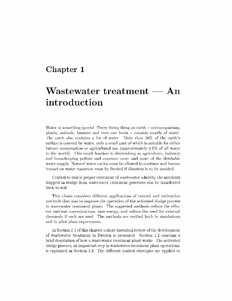
The introduction of water closets, in the beginning of the nineteenthcentury, solved many of these problems. Disease decreased and the ur-ban population avoided many problems associated with latrines; emptyinglatrine-barrels (see Figure 1.1) and bad smell. The water closet was at the�rst sight a great technical simpli�cation { waste just disappeared!
Figure 1.1: Latrine carrying in Stockholm, drawing from 1828
(Kommunf�orbundet 1988).
As an interesting sidenote, the toilet makes use of control technology.(Coury 1996). When you ush, the valve at the bottom of the tank opensand remains open because the valve oats, but when the tank is empty itcloses. Another valve then opens and water starts to �ll the tank again. Asthe water level rises a oat is carried upward which closes the oat valvewhen the tank is full. This system depends on two control loops where thewater level is used for feedback. To avoid ooding at a failure there is also
1.1 A short historical review of Swedish wastewater treatment 3
a ush valve tube inside the tank.
The use of water closets, however, soon started to a�ect the recipients1.First to be detected were the visual problems, caused by untreated wastew-ater. These were partly solved by constructing long pipes to the sea, whichin those days was believed to be capable of absorbing in�nite amounts ofwastewater. The risk of pollution and loss of fertilizer were considereda reasonable price to pay compared to the positive e�ects. The positivee�ects were also seen immediately, while the negative consequences tooklonger to detect. Almost 50 years went by before the associated pollutionproblems began to receive serious attention in Sweden.
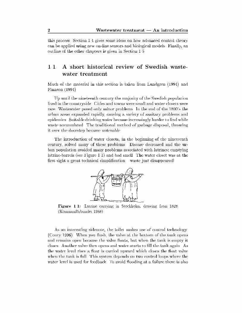
Sedimentation tanks were introduced in the 1930's to deal with thevisual problems with wastewater. By the 1950's biological treatment wasinitiated after problems began to show up with oxygen depletion in therecipients. Combined biological-chemical treatment was introduced in the1970's, due to the eutrophication of lakes from phosphorus and nitrogen inwastewater. Developments in wastewater treatment technologies between1965 and 1990 in Sweden are shown in Figure 1.2.
Figure 1.2: The development of wastewater treatment 1965{1990 in
Sweden (Hultman 1992).
1The river, lake or other watercourse where the treated wastewater is let out into.
4 Wastewater treatment | An introduction
In 1992 a European Community directive required all member statesto improve their wastewater treatment by the turn of the century. Swedenhas decided to decrease of the nitrogen discharges by approximately 50%for larger wastewater treatment plants located on the coast from Norway toStockholm. Phosphorus removal should also be increased for these plants.Further reduction of nitrogen demands more e�cient control and operationof the wastewater treatment plants. This is one of the major motivationsbehind this thesis.
1.2 A wastewater treatment plant
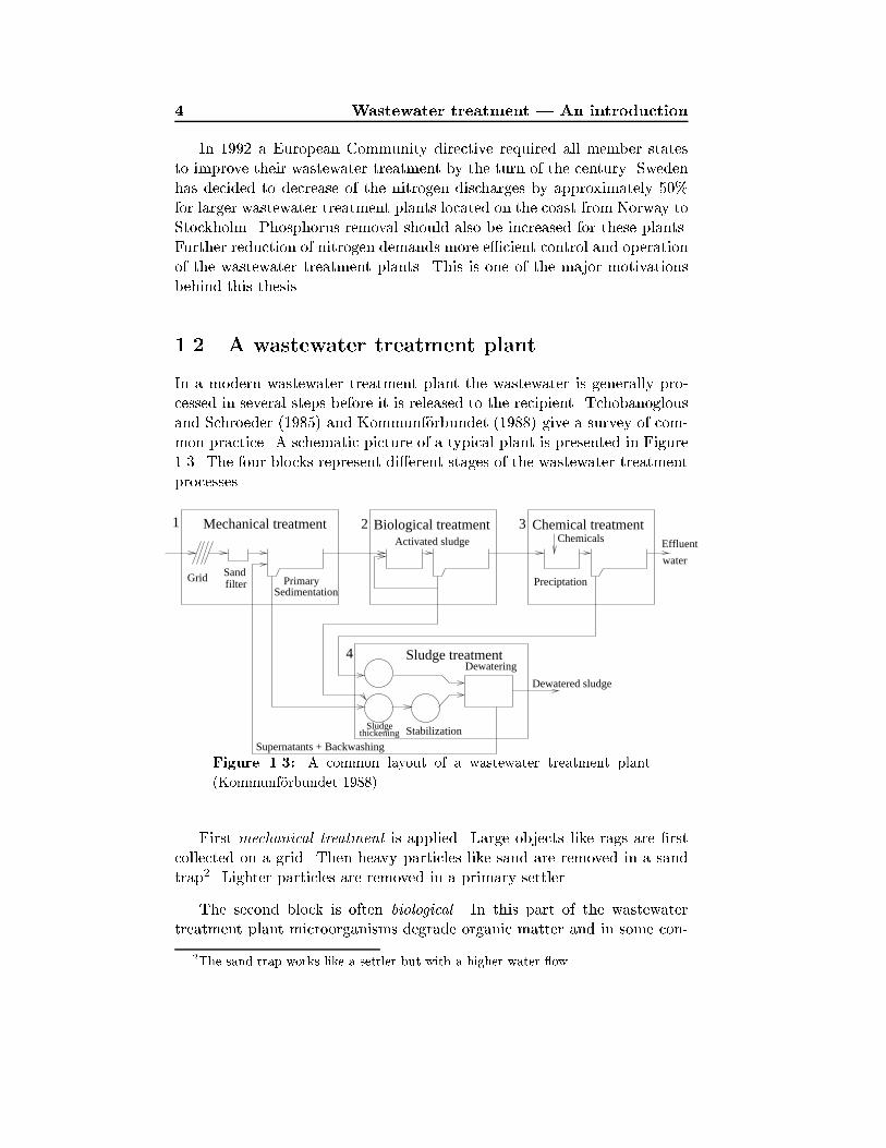
In a modern wastewater treatment plant the wastewater is generally pro-cessed in several steps before it is released to the recipient. Tchobanoglousand Schroeder (1985) and Kommunf�orbundet (1988) give a survey of com-mon practice. A schematic picture of a typical plant is presented in Figure1.3. The four blocks represent di�erent stages of the wastewater treatmentprocesses.
Chemical treatment
Sludge treatment
PrimarySedimentation
Dewatered sludge
water
Sludgethickening Stabilization
Dewatering
Biological treatment
Sandfilter
Grid
Activated sludge
Supernatants + Backwashing
Effluent
Mechanical treatment 321
4
Chemicals
Preciptation
Figure 1.3: A common layout of a wastewater treatment plant
(Kommunf�orbundet 1988).
First mechanical treatment is applied. Large objects like rags are �rstcollected on a grid. Then heavy particles like sand are removed in a sandtrap2. Lighter particles are removed in a primary settler.
The second block is often biological. In this part of the wastewatertreatment plant microorganisms degrade organic matter and in some con-
2The sand trap works like a settler but with a higher water ow.
1.2 A wastewater treatment plant 5
�gurations nutrients are also removed. Di�erent biological processes exist,but most larger wastewater treatment plants make use of the activated
sludge process. In its basic con�guration the activated sludge process con-sists of an aerated tank and a settler. The microorganisms grow slowly inthe aerated tank. In order to maintain their population sizes, sludge fromthe settler which contains microorganisms is recirculated back to the aer-ated tank. Excess sludge is removed to both avoid sludge in e�uent waterand to maintain a reasonable suspended solids concentration. Further in-formation is to be found in Section 1.3. Other types of biological treatmentare also available. An oxidation pond, for example, is a pond where thewastewater is retained for 20{40 days. During this period the wastewateris treated by microorganisms, algae, and the in uence of sunlight. Thetrickling �lter is another kind of biological treatment. It is a construction�lled with rocks or plastic objects to which the microorganisms attach andgrow. The wastewater becomes treated while it trickles through the �lter.Air is also blown through the �lter to increase the oxygen concentrationand hence improve treatment. Wetlands are yet a further biological alter-native. In a wetland, wastewater is spread out over a large area with awater depth of around 0.5 meters. Plants and microorganisms treat thewastewater. Wetlands are usually used as a �nal polishing step and notas a replacement for an activated sludge process. In this thesis only theactivated sludge process will be considered.
Phosphorus is often removed from the wastewater by chemical treat-
ment as shown in the third block of Figure 1.3. But it is also common tohave this step in the beginning { pre-precipitation. A precipitation chem-ical is added which turns phosphate into insoluble fractions. Precipitationchemicals also stimulate the creation of ocks. The insoluble phosphates aswell as organically bounded phosphate then absorb or adhere to the ocks.The ocks are separated by either sedimentation or otation. Instead ofusing chemicals, enhanced phosphorus removal can be applied in the acti-vated sludge process by biological treatment. A special con�guration of theactivated sludge process makes this possible. Henze et al. (1995b), Balm�erand Hultman (1988) and Isaacs and Henze (1995) discuss this further.
As a �nal step sometimes chlorination for disinfection and removal ofbad smell is included before the water is released in the recipient.
Sludge from the di�erent blocks is processed in the sludge treatment.The sludge consists of organic material which has to be stabilized to avoidodor and reduce the pathogenic content. The stabilization is commonlydone in anaerobic digesters. In the digesters organic matter is degraded,and most pathogenic bacteria and microorganisms die due to the high tem-
6 Wastewater treatment | An introduction
perature. Bio-gas, methane and carbon dioxide are produced during diges-tion. Before sludge is transported away it is dewatered, either mechanicallyby centrifuging, �ltering, and pressing, or by drying. This is done to reducetransportation costs since the sludge contains about 95% water. After treat-ment, sludge may be dumped or used as a fertilizer and soil conditioner. Ifthe content of heavy metals or other poisonous matter in the sludge is toohigh, it is of course not suitable to use in agricultural practice. It may alsobe used as fuel or in construction materials (Bradley et al. 1992). Lue-Hinget al. (1992) gives a more detailed description on municipal sewage sludgemanagement. The waste gathered in the grid and sand �lter, in the me-chanical treatment, is usually not treated. It is instead directly transportedto a garbage dump.
1.3 The activated sludge process
A basic description of the activated sludge process is presented. How theactivated sludge process can be extended for nitrogen removal is also ex-plained. Finally, a simple mathematical model is given.
1.3.1 Basic description
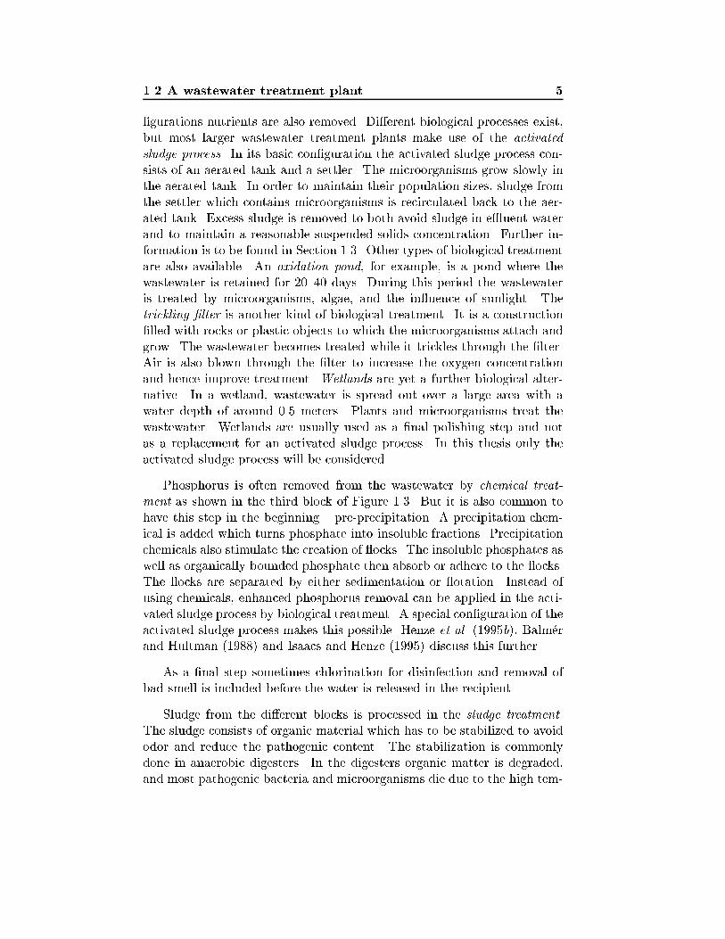
In Figure 1.4 the basic layout of an activated sludge process is shown. The
Recirculated sludge Excess sludge
Effluent waterwaterInfluent SettlerAerated tank
Figure 1.4: An activated sludge process with an aerated tank and a
sedimentation tank.
activated sludge process is a biological process in which microorganisms ox-idize and mineralize organic matter. All microorganisms enter the systemwith the in uent wastewater. The composition of the species depends notonly on the in uent wastewater but also on the design and operation of thewastewater treatment plant. Microorganisms are kept suspended either byblowing air into the tank or by the use of agitators. Oxygen is used by themicroorganisms to oxidize organic matter. To maintain the microbiologi-cal population, sludge from the settler is recirculated to the aerated tank.
1.3 The activated sludge process 7
The growth of the microorganisms and in uent particulate inert matter isremoved from the process as excess sludge. Microorganism concentrationis controlled by the excess sludge ow rate.
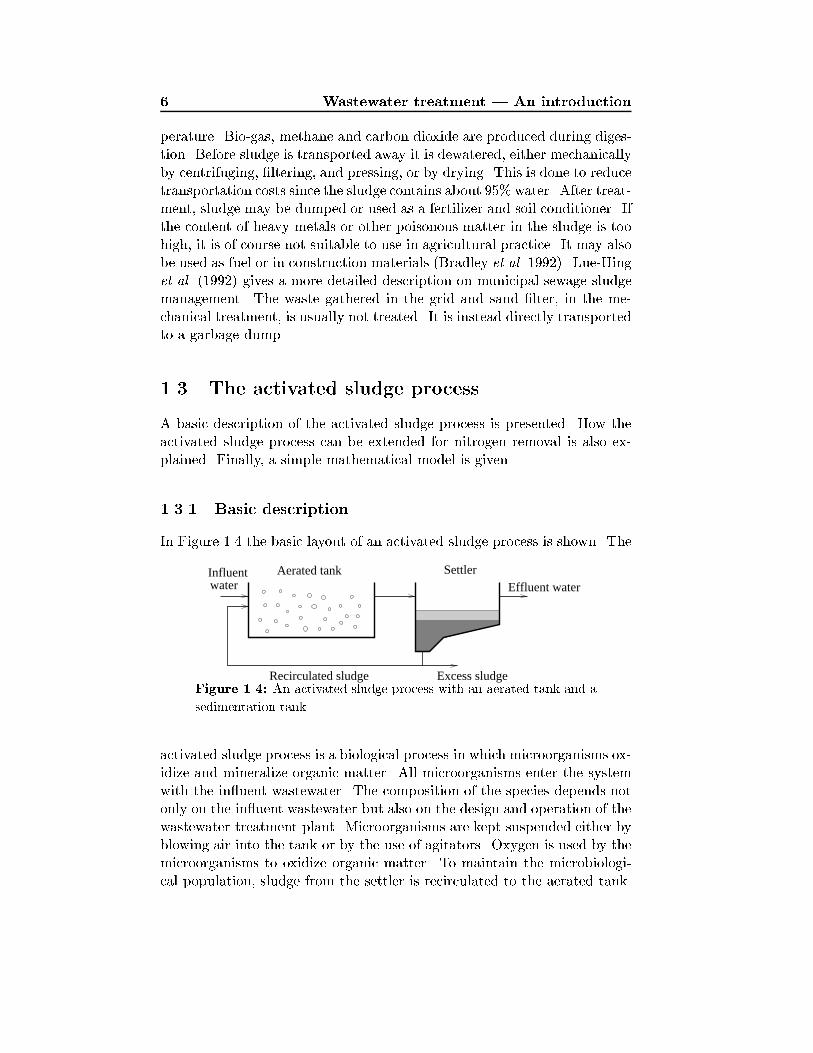
A basic model of the biological renewal process in an activated sludgeprocess is illustrated in Figure 1.5. Organic matter enters the plant inseveral di�erent forms and is converted to other forms by biological pro-cesses. Hydrolysis transforms larger organic molecules in the initial fraction
Slowly degradable material
Readily degradable material
Biomass
Inert material
Decay
Biological growth
Hydrolysis
?
?
?
-
Figure 1.5: The biological renewal process (Henze et al. 1995a).
of slowly degradable matter into smaller, more easily accessible molecules(readily degradable matter). The speed of hydrolysis may be a constraintin a wastewater treatment plant if the in uent wastewater mainly consistsof slowly biodegradable matter, since the hydrolysis process is relativelyslower than the growth rate of the microorganisms (biomass). The biomassgrowth rate depends on many variables such as the amount of biomass,the substrate, temperature, pH, and the presence of toxins. During biore-duction (decay of microorganisms), biologically inert (non-biodegradable)matter is produced. Incoming wastewater will contain some inert matteras well. This matter ows una�ected through the process and is collectedand removed in the settler.
8 Wastewater treatment | An introduction
1.3.2 Biological nitrogen removal
Nitrogen is present in several forms in wastewater, e.g. as ammonium(NH+
4 ), nitrate (NO�3 ), nitrite (NO�2 ) and as organic compounds. Nitro-
gen is an essential nutrient for biological growth and is one of the mainconstituents in all living organisms. The presence of nitrogen in e�uentwastewater, however, presents many problems (Barnes and Bliss 1983).
� Ammonia (NH3) is toxic to aquatic organisms, especially for higherlife forms such as �sh.
� When ammonium is oxidized to nitrate, a signi�cant oxygen demandin the receiving water may give rise to a severe depletion of the dis-solved oxygen concentration.
� Nitrite in drinking water is toxic, especially for human infants.
� Nitrogen is a nutrient stimulating growth of aquatic plants. Whenthe plants die, oxygen is consumed by organisms degrading the litter.
� The presence of ammonium in the drinking water supply requires anincreased chlorine dosages.
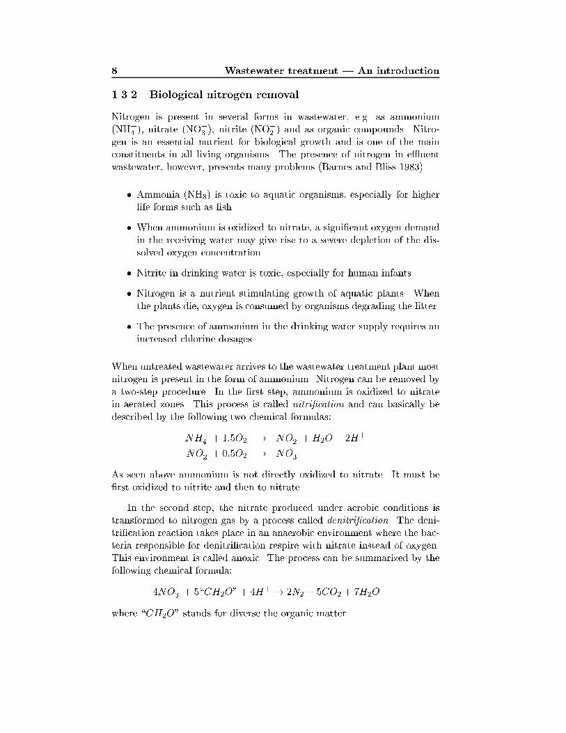
When untreated wastewater arrives to the wastewater treatment plant mostnitrogen is present in the form of ammonium. Nitrogen can be removed bya two-step procedure. In the �rst step, ammonium is oxidized to nitratein aerated zones. This process is called nitri�cation and can basically bedescribed by the following two chemical formulas:
NH+4 + 1:5O2 ! NO�2 +H2O + 2H+
NO�2 + 0:5O2 ! NO�3
As seen above ammonium is not directly oxidized to nitrate. It must be�rst oxidized to nitrite and then to nitrate.
In the second step, the nitrate produced under aerobic conditions istransformed to nitrogen gas by a process called denitri�cation. The deni-tri�cation reaction takes place in an anaerobic environment where the bac-teria responsible for denitri�cation respire with nitrate instead of oxygen.This environment is called anoxic. The process can be summarized by thefollowing chemical formula:
4NO�3 + 5\CH2O" + 4H+ ! 2N2 + 5CO2 + 7H2O
where \CH2O" stands for diverse the organic matter.
1.3 The activated sludge process 9
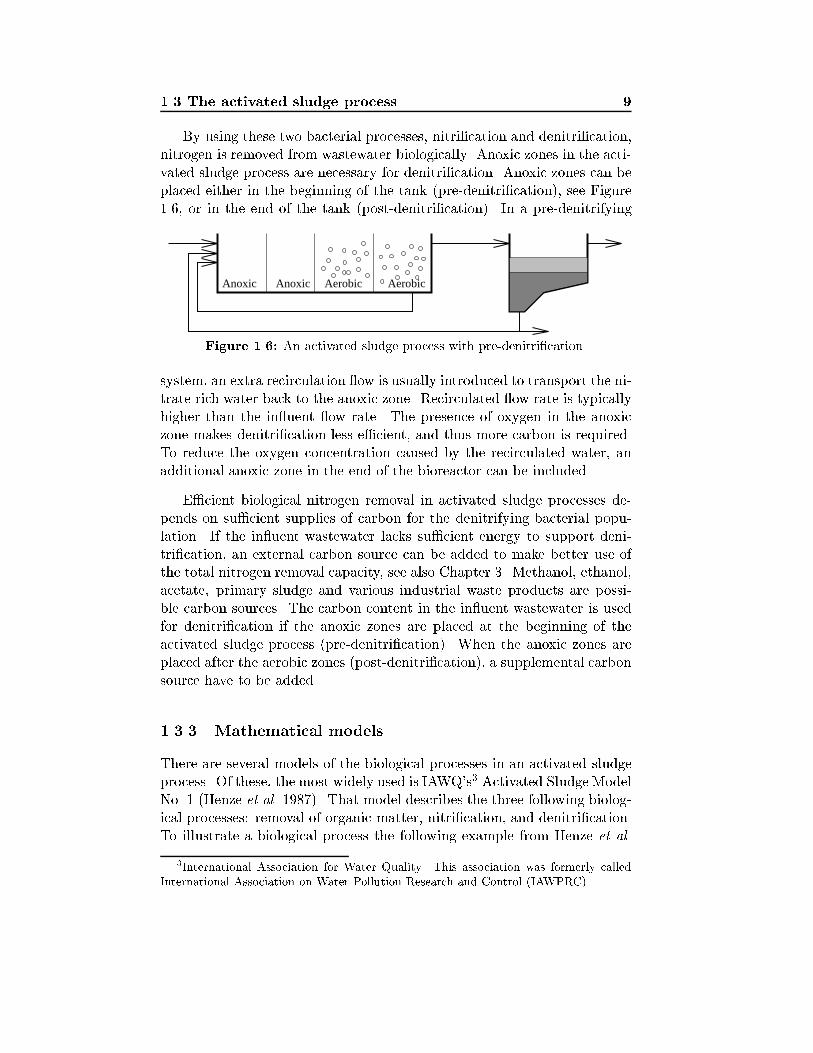
By using these two bacterial processes, nitri�cation and denitri�cation,nitrogen is removed from wastewater biologically. Anoxic zones in the acti-vated sludge process are necessary for denitri�cation. Anoxic zones can beplaced either in the beginning of the tank (pre-denitri�cation), see Figure1.6, or in the end of the tank (post-denitri�cation). In a pre-denitrifying
Anoxic Anoxic Aerobic Aerobic
Figure 1.6: An activated sludge process with pre-denitri�cation.
system, an extra recirculation ow is usually introduced to transport the ni-trate rich water back to the anoxic zone. Recirculated ow rate is typicallyhigher than the in uent ow rate. The presence of oxygen in the anoxiczone makes denitri�cation less e�cient, and thus more carbon is required.To reduce the oxygen concentration caused by the recirculated water, anadditional anoxic zone in the end of the bioreactor can be included.
E�cient biological nitrogen removal in activated sludge processes de-pends on su�cient supplies of carbon for the denitrifying bacterial popu-lation. If the in uent wastewater lacks su�cient energy to support deni-tri�cation, an external carbon source can be added to make better use ofthe total nitrogen removal capacity, see also Chapter 3. Methanol, ethanol,acetate, primary sludge and various industrial waste products are possi-ble carbon sources. The carbon content in the in uent wastewater is usedfor denitri�cation if the anoxic zones are placed at the beginning of theactivated sludge process (pre-denitri�cation). When the anoxic zones areplaced after the aerobic zones (post-denitri�cation), a supplemental carbonsource have to be added.
1.3.3 Mathematical models
There are several models of the biological processes in an activated sludgeprocess. Of these, the most widely used is IAWQ's3 Activated Sludge ModelNo. 1 (Henze et al. 1987). That model describes the three following biolog-ical processes: removal of organic matter, nitri�cation, and denitri�cation.To illustrate a biological process the following example from Henze et al.
3International Association for Water Quality. This association was formerly calledInternational Association on Water Pollution Research and Control (IAWPRC).
10 Wastewater treatment | An introduction
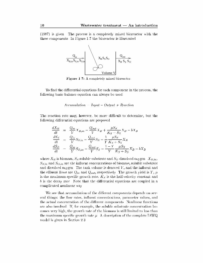
(1987) is given. The process is a completely mixed bioreactor with thethree components. In Figure 1.7 the bioreactor is illustrated.
Volume V
Q QX S SSB O
in out
X S SB,in S,in X S SS OO,in B
Figure 1.7: A completely mixed bioreactor.
To �nd the di�erential equations for each component in the process, thefollowing basic balance equation can always be used.
Accumulation = Input { Output + Reaction
The reaction rate may, however, be more di�cult to determine, but thefollowing di�erential equations are proposed
dXB
dt=
Qin
VXB;in � Qout
VXB +
�SSKS + SS
XB � bXB
dSSdt
=Qin
VSS;in � Qout
VSS � 1
Y
�SSKS + SS
XB
dSOdt
=Qin
VSO;in � Qout
VSS � 1� Y
Y
�SSKS + SS
XB � bXB
where XB is biomass, SS soluble substrate and SO dissolved oxygen. XB;in,SS;in and SO;in are the in uent concentrations of biomass, soluble substrateand dissolved oxygen. The tank volume is denoted V , and the in uent andthe e�uent ows are Qin and Qout, respectively. The growth yield is Y , �is the maximum speci�c growth rate, KS is the half-velocity constant andb is the decay rate. Note that the di�erential equations are coupled in acomplicated nonlinear way.
We see that accumulation of the di�erent components depends on sev-eral things: the ow rates, in uent concentrations, parameter values, andthe actual concentration of the di�erent components. Nonlinear functionsare also involved. If, for example, the soluble substrate concentration be-comes very high, the growth rate of the biomass is still limited to less thanthe maximum speci�c growth rate �. A description of the complete IAWQmodel is given in Section 2.3.
1.4 Control of wastewater treatment plants 11
1.4 Control of wastewater treatment plants
The allowed levels of pollutants in treated wastewater have become in-creasingly stringent with time. Taking into account current environmentalproblems, it is not unrealistic to believe that the this trend will continue. Atthe same time loads on existing plants plants are expected to increase dueto growth of urban areas. This situation demands more e�cient treatmentprocedures for wastewater.
One way to improve e�ciency could be to construct new and largerbasins, but this is expensive and often impossible since the land requiredis just not available. Another way would be the introduction of more ad-vanced control and operating systems. This is expected to reduce the needfor larger volumes, improve the e�uent water quality, decrease the use ofchemicals, and save energy and operational costs. Sustainable solutionsto the problems of wastewater treatment will require the development ofadequate information systems for control and supervision of the process.
Today many wastewater treatment plants use very simple control tech-nologies or no automatic control at all. Control techniques in current use in-clude simple PLC-techniques, time control, manual control, rules of thumb,or simple proportional control. Advanced models of the processes in awastewater plant such as the IAWQ's Activated Sludge Model No. 1 havebeen developed over the years, but have not been used to any extent forpractical control design. It is di�cult to design a sensible controller basedon the IAWQ model, which is nevertheless a very useful model to evaluatedi�erent control strategies. Several advanced control strategies have pre-viously been suggested, see e.g. Bastin and Dochain (1990), Van Impe etal. (1992), Dochain and Perrier (1993), Nielsen and Lynggaard (1993), andYoussef et al. (1995).
The following reasons may explain why advanced control have not beenextensively used. (See Olsson (1993a) for a more throughly treatment ofthe subject.)
� The e�uent standards have not been tight enough. Economic penal-ties for exceeding the regulations along with stricter e�uent regula-tions which are not based solely on long average values could encour-age implementation of better control.
� Wastewater treatment is often considered as a non-productive pro-cess. Since control systems are expensive it may be di�cult to con-vince a manager to introduce a more advanced system, especiallywhen pro�t can not be guaranteed.
12 Wastewater treatment | An introduction
� On-line sensors have been unreliable and require a lot of maintenance.
� Many pumps, valves, and other actuators are not controllable; oftenthey can only be switched on or o�.
� The process is very complex and it is not obvious how to control andoptimize the plant.
� Few control engineers have devoted their attention to wastewatertreatment plants.
Interest for applying more sophisticated control is, however, growing.The reasons for this are most economical:
� Cost e�ective solutions are becoming more and more important. Asthe loads on existing plants increase, control and optimization maybe able to handle the increasing loads with the same volumes.
� Sti�er requirements on treated wastewater.
� Fees and taxes related to the e�uent water quality are making it moreexpensive to release pollutions.
� The general public's awareness of environmental issues is increasingand more and more focused on issues of sustainability and energyconsumption.
� Improved on-line sensors and actuators are being continuously devel-oped.
� More complex process alternatives, which are di�cult to control man-ually.
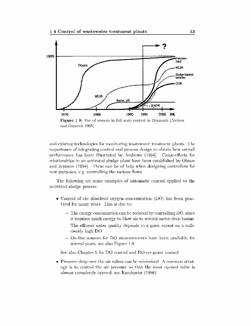
Application of modern control theory in combination with new on-linesensors and the appropriate parts of advanced models has great potentialto improve the e�uent water quality, decrease the use of chemicals and tosave energy and money, see Van Impe et al. (1992), Carlsson (1995), andCarlsson (1997) for more discussions. Nielsen and �Onnerth (1995) suggestan expert system which use on-line sensors to control and optimize the plantperformance. They also give a short overview of the development of on-linesensors over the last 25 years. The use of on-line sensors has increasedrapidly in the last years, see Figure 1.8. This trend is expected to continuedue to the large potential for reducing costs when used in combinationwith automatic control. Vanrolleghem and Verstraete (1993) surveyed new
1.4 Control of wastewater treatment plants 13
Figure 1.8: Use of sensors in full-scale control in Denmark (Nielsen
and �Onnerth 1995).
and existing technologies for monitoring wastewater treatment plants. Theimportance of integrating control and process design to obtain best overallperformance has been illustrated by Andrews (1994). Cause-e�ects forrelationships in an activated sludge plant have been established by Olssonand Jeppson (1994). These can be of help when designing controllers fornew purposes, e.g. controlling the various ows.
The following are some examples of automatic control applied to theactivated sludge process.
� Control of the dissolved oxygen concentration (DO) has been prac-ticed for many years. This is due to:
{ The energy consumption can be reduced by controlling DO, sinceit requires much energy to blow air to several meter deep basins.
{ The e�uent water quality depends to a great extent on a su�-ciently high DO.
{ On-line sensors for DO measurements have been available forseveral years, see also Figure 1.8.
See also Chapter 5 for DO control and DO set-point control.
� Pressure drop over the air valves can be minimized. A common strat-egy is to control the air pressure so that the most opened valve isalmost completely opened, see Rundqwist (1986).
14 Wastewater treatment | An introduction
� The nitrate concentration can be kept low by adding an external car-bon source. Using on-line measurements of the nitrate concentration,a proper ow rate of the external carbon source can be given, seeHellstr�om and Bosander (1990), and Isaacs et al. (1993). By usingfeedforward control from in uent total organic carbon (TOC) andrecirculated nitrate, disturbances in in uent water can be better re-jected, Chapter 3 discuss this.
� It is important to control the chemical dosage in a wastewater plant.Phosphorus, for example, is removed by chemical precipitation. Acombination of feedback and feedforward control from on-line sensors, ow rates and an experience data base may be useful to maintainappropriate chemical dosages.
� The ammonium concentration can be controlled by the DO set-pointand/or the number of aerated zones. This is an alternative to using a�xed DO set-point, see Nielsen and Lynggaard (1993), and Chapter3.
� Optimizing the di�erent ow rates in the plant is an interesting �eldof research, see e.g. Nielsen and Lynggaard (1993), and Vanrolleghem(1994). Some of the ows determine the amount of biomass in the sys-tem. Maintaining a high concentration of biomass is a tempting strat-egy to improve plant performance, since a large biomass can degrademore organic material. Unfortunately, the sedimentation propertiescan be a�ected detrimentally and foam can also be created. Otherforms of microorganisms may also adapt to the high concentration ofbiomass, which in turn makes the activated sludge process less e�-cient. At present it is, however, di�cult to predict how an increasedsludge concentration will in uence sludge sedimentation properties.
� In uent ow can to some extent be controlled by constructing ad-ditional tanks or using the large wastewater tunnels as reservoirs.The large variations in the in uent wastewater ow can then be sig-ni�cantly reduced. Variations in in uent ow are mainly caused byrain water leaking into the pipes, or by drainage water. This typeof variation forces plants to work with higher ows during short pe-riods which is less e�cient compared to a constant ow. Sometimesone also has to do by-pass actions to avoid sludge loss from the sec-ondary clari�er. There have been experiments in G�oteborg where thewastewater tunnels were used as reservoirs (Gustafsson et al. 1993).Also, outside Malm�o (Nyberg et al. 1996) and in Denmark (Nielsenet al. 1996), similar trials have been done to avoid problems duringhigh in uent ow rates.
1.4 Control of wastewater treatment plants 15
� The clari�er has the dual task of clarifying and thickening the sludge.Its function is crucial to the operation of the activated sludge process.Hence modeling, diagnostics, and control of the sedimentation processare also important topics, see e.g. Jeppsson (1996), and Bergh (1996).
� The activated sludge process is a multivariable process, i.e. it hasseveral inputs (control handles) and several outputs. There are alsomany cross couplings. If, for example, the DO set-point is changed,both the ammonium and nitrate concentrations are a�ected. If theinternal recirculation is varied, this a�ects several parameters in theprocess. Hence a multivariable controller which can use cross cou-plings e�ciently, may be useful to optimize the plant performance.Dochain and Perrier (1993), and Chapter 6 take this up.
� A key goal in wastewater treatment is to maintain e�uent qualitystandards at a minimum cost. Obviously, it is not enough to havean e�ective control of various subprocesses. One must also considervarious types of supervision control based on some cost function. Suchstrategies have been discussed by Vanrolleghem et al. (1996).
� Control theories may also be used to design software sensors for esti-mating the respiration rate from measurements of the dissolved oxy-gen concentration and air ow rate, see Chapter 4.
The above list of control strategies for wastewater treatment is by no meanscomplete. More ideas, examples and motivations can, for instance, be foundin the IAWQ proceedings of the workshops in Instrumentation, Controland Automation of Water and Wastewater Treatment and TransportationSystems.
New control strategies may involve the use of simpli�ed biological/physicalmodels, feedforward control from measurable disturbances, simple estima-tion models, supervision control, and real-time estimation.
For a control engineer the activated sludge process in a wastewatertreatment plant is a challenging topic for several reasons.
� The process is time-varying. It is a biological process where temper-ature, composition of in uent water, amount of biomass, ows, etc,vary in time.
� The process is non-linear and time-varying. Several things make theprocess (model) nonlinear, e.g. the Monod functions ( �SS
KS+SS), and
16 Wastewater treatment | An introduction
multiplication of states (bilinearity). The pump ows, which variesin time, make the dynamic time-varying.
� The process has sti� dynamics. It has time constants which rangefrom seconds to months. This may not have to be a major problemsince cascade control may be applied. Cascade control means that afast controller controls a fast sub-process and a slower controls theset-point of the fast controller.
� The process is multivariable. The process has several inputs andoutputs. What should be considered as inputs and outputs are notobvious. An input could, for example, be a set-point for a fast con-troller, and an output does not necessarily have to be a concentrationin the e�uent, it could be a concentration in a zone. There are alsolarge cross-couplings, e.g. if a ow is changed, many other variablesare a�ected.
� Many sensors are still not reliable. Much progress has been made insensor development in recent years. Common problems are that thesensors are fairly noisy, have long response times, require frequentmaintenance, and that they drift.
� Large disturbances a�ect the process. Especially in uent ow andin uent concentrations are subject to large variation.
1.5 Outline of the thesis
In this section a brief summary of the main contributions in the thesis ispresented. Note that each chapter contains a review of previous research.
In chapter 2 the pilot plant is presented. The pilot plant was designedto study new methods for e�cient nutrient removal using advanced processtechnology, applied microbiology and automatic control. It is controlled byan advanced control and supervision system (CSS), where the user can viaa graphical interface operate the plant, control data acquisition, save andplot data, respond to alarms and tune controllers. The CSS was developedas a Masters project (Latomaa 1994), where I have been co-supervisor.A simulator based on the control and supervision system has been thesubject of another Masters project (Luttmer 1995), where I also have beenco-supervisor. The simulator's main function is to run simulations on anactivated sludge process. As such, the simulator is an e�ective teachingaid.
1.5 Outline of the thesis 17
A simulation model is also presented in Chapter 2. This model is usedin most simulations in this thesis. It is an approximation of the pilot plant,and the same volumes and ows are also used. The parameters in the modelare, however, not calibrated to the real process. Prior experiments with thepilot plant, simulations are very useful to evaluate control strategies, or testdi�erent controllers.
An external carbon source can increase the denitri�cation rate and com-pensate for de�ciencies in the in uent carbon/nitrogen ratio. In Chapter 3the problem of controlling the ow rate of an external carbon source is con-sidered. The control strategy for the carbon dosage is based on keeping thenitrate level in the anoxic zone at a constant and low level. To better rejectdisturbances, feedforward from the mass ow of in uent TOC and recircu-lated nitrate are used. Four di�erent types of feedforward controllers areevaluated: a PID-controller, a direct adaptive controller, an indirect adap-tive controller, and a model-based adaptive PID controller. The controllersare compared in a simulation study, and the direct adaptive controller isfurther tested in the pilot plant. Additionally a number of problems andtheir solutions concerning adaptive control are discussed in this chapter.
In Chapter 4, methods for estimating two essential parameters whichcharacterize the dissolved oxygen concentration (DO) dynamics in an acti-vated sludge process are presented. The two variables are the respirationrate R(t), and the oxygen transfer function KLa. The respiration rate is akey variable that characterizes the DO process and the associated removaland degradation of biodegradable matter. The oxygen transfer functionKLa describes the rate with which oxygen is transferred to the activatedsludge by the aeration system. The KLa function is expected to be a non-linear function of the air ow rate. The estimation algorithm is based ona Kalman �lter which uses measurements of the dissolved oxygen concen-tration and air ow rate. To improve estimation, di�erent models of thetime-varying respiration rate and nonlinear oxygen transfer function havebeen developed, and evaluated in a simulation study and on real data. Ifthe DO sensor has dynamic, this must be taken into account, otherwisethe estimates will be biased. A �lter which compensates for the DO sensordynamic has been designed. This �lter is not only useful for DO measure-ments, it can be applied to any sensor where there is need for compensationof the sensor dynamic. In a Masters project (Nakajima 1996), where I havebeen a co-supervisor, an extended Kalman �lter was utilized, instead ofthe suggested �lter to compensate for the sensor dynamic. Surfactantsmay reduce the oxygen transfer function KLa. The suggested estimationalgorithm has been used to study the e�ect surfactants has on KLa. BothKLa and the respiration rate were found to be reduced by the addition
18 Wastewater treatment | An introduction
of a surfactant. An improvement over previous methods, this estimationalgorithm is capable of both estimating a nonlinear KLa function and atime-varying respiration rate. Further, the �lter which compensates forthe sensor dynamics has tuning knobs for both smoothing lag and noisesensitivity.
The estimated nonlinear oxygen transfer function is used to design anonlinear controller of the dissolved oxygen concentration in Chapter 5.The DO in the aerobic part of an activated sludge process should be suf-�ciently high in order for microorganisms to degrade organic matter andconvert ammonium to nitrate. On the other hand, an excessively high DO,which requires a high air ow rate, results in high energy consumption andmay even deteriorate sludge quality. Control of the DO is therefore im-portant. Since the KLa function is nonlinear, the gain of the process willvary with varying air ow rate. By designing a nonlinear controller, a com-pensation for the nonlinearity can be made and high control performancemay be obtained under all operating conditions. Simulations and practi-cal experiments con�rm these results. An outline for DO set-point controlare given. Its purpose is to control the ammonium concentration in theaerated zone by the DO set-point. An experiment in the pilot plant withthe set-point controller showed that it was not only possible to save energydue to a lower DO set-point, the e�uent nitrate concentration was alsosigni�cantly reduced. Possible disadvantages may be that sludge proper-ties deteriorate due to the low DO, and nitrous oxide (N2O) can be formedwhen the DO is low. These problems should, however, be compared to theachieved improvements. Spatial DO set-point control may also reduce thisproblem by switching o� aeration in some zones when the DO set-pointbecomes too low. The DO set-point can then be increased in the remainingzones. A pressure controller is �nally presented in this chapter. The idea,which is well known, is to control air pressure so that the most open airvalve becomes almost completely open. This was later con�rmed in thepilot plant.
Multivariable linear quadratic (LQ) controllers are designed in Chapter6. The controllers are based on a linear state-space model estimated by asubspace system identi�cation method. The main advantage of these con-trollers, compared to SISO controllers, are that they take all interactions inthe process model into account. This allows for a sensible trade o� betweenthe di�erent control handles and outputs. The following inputs are used:external carbon, internal recirculation rate, and DO set-point. Ammoniumand nitrate in the last aerated zone are used as outputs. The controllersoutlined also use feedforward from the measurable disturbances: in uent ow rate, in uent ammonium and in uent carbon. The two di�erent mul-
1.5 Outline of the thesis 19
tivariable controllers have been evaluated in a simulation study. One of thecontrollers is based on di�erentiating the states, and the other has addi-tional integration states. Both controllers have shown good performance insimulations. It was, however, found that the modeling part was crucial forthe control performance.
Conclusions and some topics for future research are summarized inChapter 7. Means of optimizing the activated sludge process using eco-nomic cost functions discussed are discussed. By setting prices on thee�uent discharges, and on the control variables, i.e. blowing air, dosing ex-ternal carbon, running pumps, etc., the most economically way to run theplant can be determined. Parts of this strategy could also be implementedin an extremum controller. Further discussions involves how wastewatertreatment plants can be divided in di�erent sub-processes, where each sub-process then are optimized separately.

20 Wastewater treatment | An introduction
Chapter 2
Pilot plant and simulation
model
This chapter describes the pilot-scale activated sludge plant at the mainmunicipal wastewater treatment plant in Uppsala, Sweden, and a simula-tion model of the pilot plant.
The pilot plant consists of two separate lines for pre-denitri�cation.The main purpose of the plant has been to study new methods for e�cientnutrient removal using advanced process technology, applied microbiologyand automatic control. Both lines are extensively monitored by on-line in-struments and sampling programs. The plant is controlled by an advancedcontrol and supervision system, where the user can via a graphical interfaceoperate the plant, control data acquisition, save and plot data, respond toalarms and tune controllers.
To numerically evaluate di�erent controllers and control strategies it isimportant to use a model which realistically simulates a true plant. A sim-ulation model of the pilot plant has therefore been designed. The IAWQ'sActivated Sludge Model No. 1. (Henze et al. 1987) has been used to modeleach zone of the bioreactor and the clari�cation-thickening model in Tak�acset al. (1991) has been used to model the settler.
This chapter is organized as follows. In the next section, a generaldescription of the pilot plant and its instrumentation is given. The plantis controlled by a control and supervision system which is presented inSection 2.1.2. A simulator, based on the control and supervision systemhas been designed, and is outlined in Section 2.1.3. The di�erent conductedexperiment are presented in Section 2.2. A model of the pilot plant is
22 Pilot plant and simulation model
presented in Section 2.3.1, and the bioreactor model of each zone in the pilotplant is given in Section 2.3.2. The di�erential equations and parametervalues for the activated sludge process are presented in Section 2.3.3. Thesettler model, simulation tool, and conclusions are given in Sections 2.3.4,2.3.5 and 2.3.6, respectively.
2.1 The pilot plant
2.1.1 General layout of the pilot plant
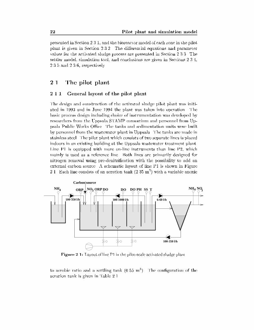
The design and construction of the activated sludge pilot plant was initi-ated in 1993 and in June 1994 the plant was taken into operation. Thebasic process design including choice of instrumentation was developed byresearchers from the Uppsala STAMP consortium and personnel from Up-psala Public Works O�ce. The tanks and sedimentation units were builtby personnel from the wastewater plant in Uppsala. The tanks are made instainless steel. The pilot plant which consists of two separate lines is placedindoors in an existing building at the Uppsala wastewater treatment plant.Line P1 is equipped with more on-line instruments than line P2, whichmainly is used as a reference line. Both lines are primarily designed fornitrogen removal using pre-denitri�cation with the possibility to add anexternal carbon source. A schematic layout of line P1 is shown in Figure2.1. Each line consists of an aeration tank (2.35 m3) with a variable anoxic
DOORP DO TSSNO ORPNH4 3
300-1000 l/h100-350 l/h
100-350 l/h
6-60 l/h
PHDO NH4 NO3
Carbon source
Figure 2.1: Layout of line P1 in the pilot-scale activated sludge plant.
to aerobic ratio and a settling tank (0.55 m3). The con�guration of theaeration tank is given in Table 2.1.
2.1 The pilot plant 23
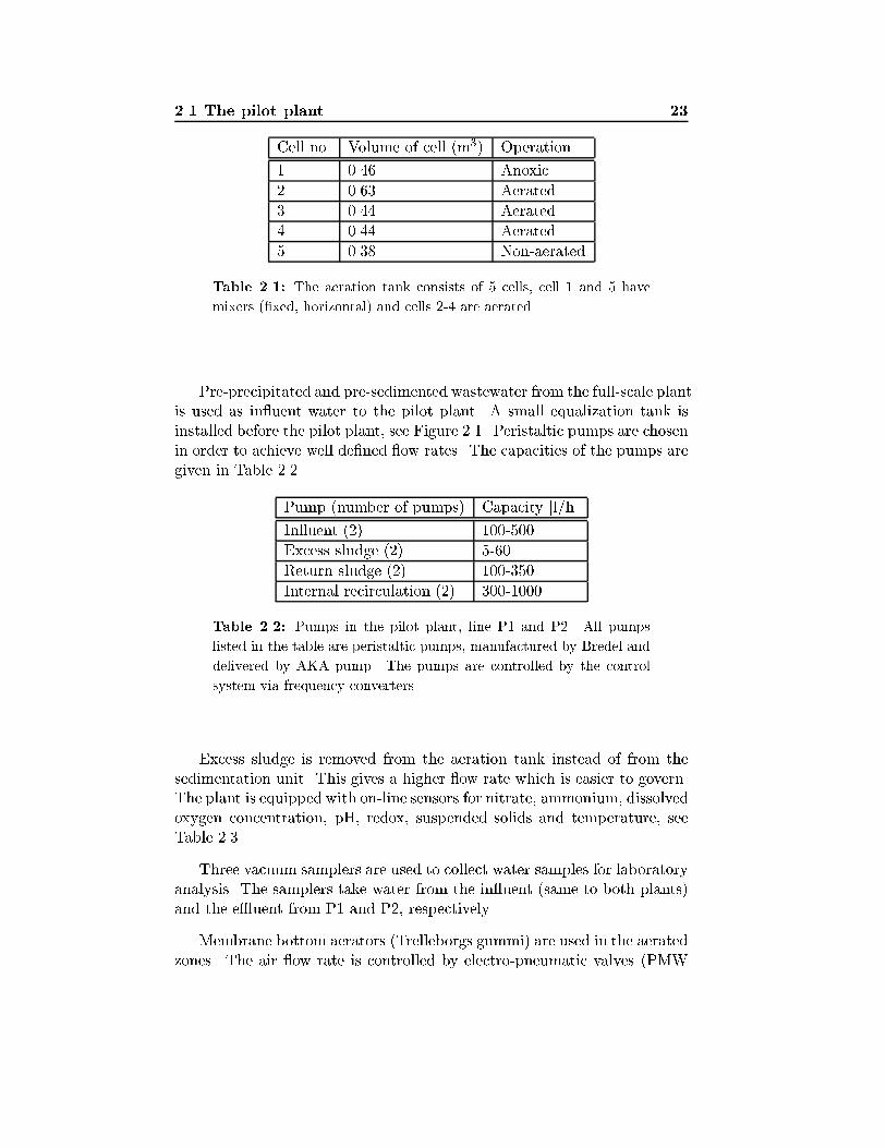
Cell no. Volume of cell (m3) Operation
1 0.46 Anoxic
2 0.63 Aerated
3 0.44 Aerated
4 0.44 Aerated
5 0.38 Non-aerated
Table 2.1: The aeration tank consists of 5 cells, cell 1 and 5 have
mixers (�xed, horizontal) and cells 2-4 are aerated.
Pre-precipitated and pre-sedimented wastewater from the full-scale plantis used as in uent water to the pilot plant. A small equalization tank isinstalled before the pilot plant, see Figure 2.1. Peristaltic pumps are chosenin order to achieve well de�ned ow rates. The capacities of the pumps aregiven in Table 2.2.
Pump (number of pumps) Capacity [l/h]
In uent (2) 100-500
Excess sludge (2) 5-60
Return sludge (2) 100-350
Internal recirculation (2) 300-1000
Table 2.2: Pumps in the pilot plant, line P1 and P2. All pumps
listed in the table are peristaltic pumps, manufactured by Bredel and
delivered by AKA pump. The pumps are controlled by the control
system via frequency converters.
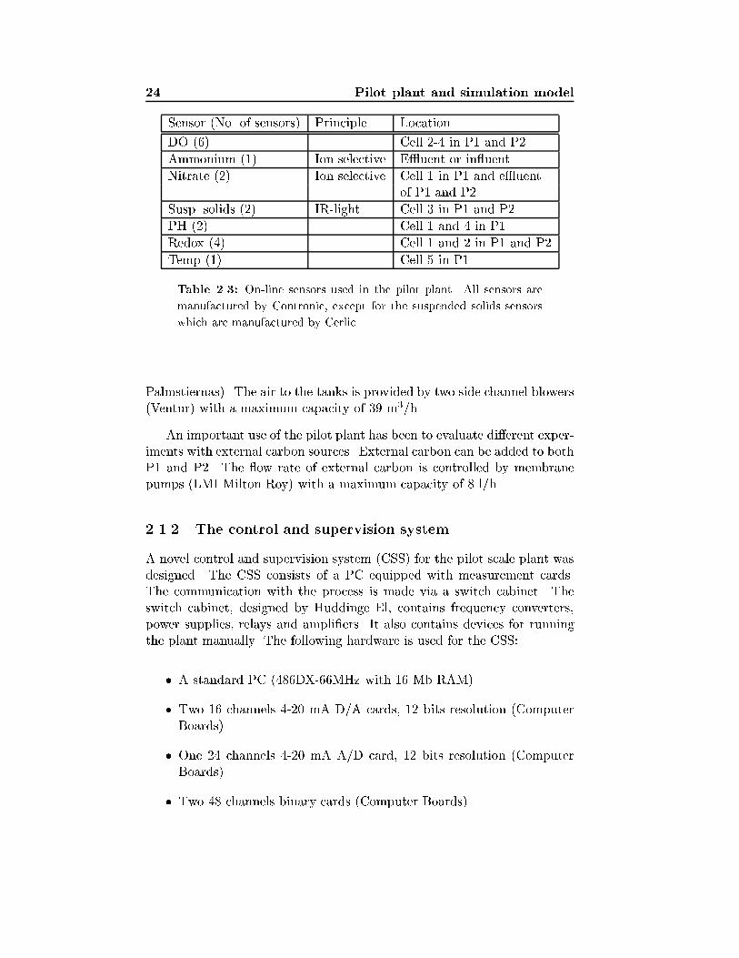
Excess sludge is removed from the aeration tank instead of from thesedimentation unit. This gives a higher ow rate which is easier to govern.The plant is equipped with on-line sensors for nitrate, ammonium, dissolvedoxygen concentration, pH, redox, suspended solids and temperature, seeTable 2.3.
Three vacuum samplers are used to collect water samples for laboratoryanalysis. The samplers take water from the in uent (same to both plants)and the e�uent from P1 and P2, respectively.
Membrane bottom aerators (Trelleborgs gummi) are used in the aeratedzones. The air ow rate is controlled by electro-pneumatic valves (PMW
24 Pilot plant and simulation model
Sensor (No. of sensors) Principle Location
DO (6) Cell 2-4 in P1 and P2
Ammonium (1) Ion selective E�uent or in uent
Nitrate (2) Ion selective Cell 1 in P1 and e�uentof P1 and P2
Susp. solids (2) IR-light Cell 3 in P1 and P2
PH (2) Cell 1 and 4 in P1
Redox (4) Cell 1 and 2 in P1 and P2
Temp (1) Cell 5 in P1
Table 2.3: On-line sensors used in the pilot plant. All sensors are
manufactured by Contronic, except for the suspended solids sensors
which are manufactured by Cerlic.
Palmstiernas). The air to the tanks is provided by two side channel blowers(Ventur) with a maximum capacity of 39 m3/h.
An important use of the pilot plant has been to evaluate di�erent exper-iments with external carbon sources. External carbon can be added to bothP1 and P2. The ow rate of external carbon is controlled by membranepumps (LMI Milton Roy) with a maximum capacity of 8 l/h.
2.1.2 The control and supervision system
A novel control and supervision system (CSS) for the pilot scale plant wasdesigned. The CSS consists of a PC equipped with measurement cards.The communication with the process is made via a switch cabinet. Theswitch cabinet, designed by Huddinge El, contains frequency converters,power supplies, relays and ampli�ers. It also contains devices for runningthe plant manually. The following hardware is used for the CSS:
� A standard PC (486DX-66MHz with 16 Mb RAM)
� Two 16 channels 4-20 mA D/A cards, 12 bits resolution (ComputerBoards)
� One 24 channels 4-20 mA A/D card, 12 bits resolution (ComputerBoards)
� Two 48 channels binary cards (Computer Boards)

2.1 The pilot plant 25
Linux, a public domain UNIX dialect was chosen as operating system. Mostof the programming was made as a Master thesis work, see Latomaa (1994).The CSS was implemented in C++ and separated into two di�erent pro-cesses which communicate through a common memory area. One processhandles the actual control of the plant, i.e. start and stop of pumps, cal-culation of control signals, collection of data, checking alarms, etc. Theother process manages the graphical user interface (GUI). The GUI wasprogrammed by using Motif. Special attention was made to create a user-friendly interface which should be easy to interpret and e�ectively presentthe status of the plant, see Carlsson and Lindberg (1995) and Carlssonet al. (1994b). The user can via the GUI operate the plant and performother tasks such as control data acquisition, plot data, respond to alarms,tune controllers, etc. Data from the on-line sensors are stored every 10thminute (averaged values are computed if the process is sampled faster than10 min).
The plant is schematically drawn in the GUI, see Figure 2.2. The owrate of a pump is changed by clicking on the pump symbol and then enteringthe ow rate. The pump symbol also indicates if the pump is switched o�,is in auto or manual mode, or if there is a pump failure. The DO iscontrolled by varying the position of the air valves. The valve opening isusually controlled by PID controllers, but more advanced control schemeswere evaluated in the experiments.
One interesting feature in the GUI is that the width of the pipes in thedrawing is proportional to the actual ow rate in the plant, see also Olsson(1993b). To further improve the presentation of the status of the plant,staples, \pie-charts" and color coding are used.
For more information about the pilot plant, see Carlsson et al. (1997).
2.1.3 A simulator based on the control and supervision sys-tem
A simulator for an activated sludge process has been designed. What isspecial with this simulator compared to other simulators, is that the pre-vious outlined control and supervision system is used. This means thatthe same user friendly GUI is used. It is hence very easy to, for example,change pump ow rates, DO set-points or carbon dosage. It is also easy toplot the di�erent concentrations and vary the composition of the in uentwastewater. The only di�erence to the GUI in the CSS is that a simulatedprocess is controlled instead of the pilot scale plant, and the simulationruns of course much faster than the processes in the pilot scale plant.
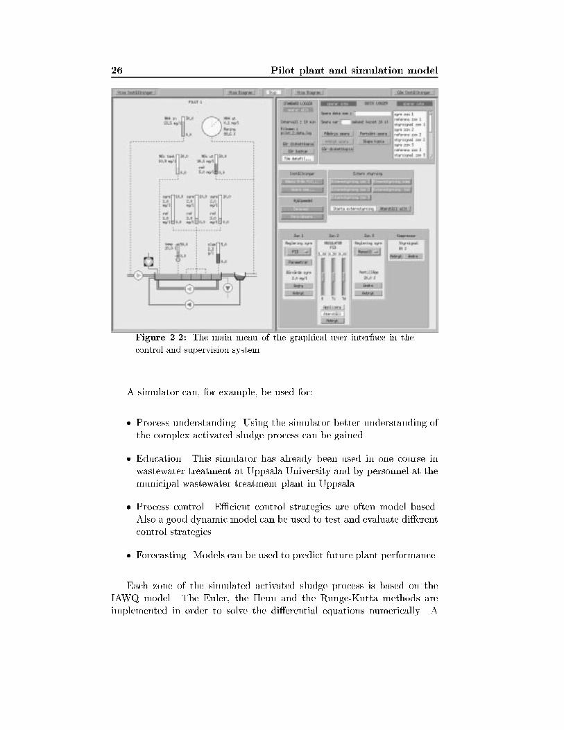
26 Pilot plant and simulation model
Figure 2.2: The main menu of the graphical user interface in the
control and supervision system.
A simulator can, for example, be used for:
� Process understanding. Using the simulator better understanding ofthe complex activated sludge process can be gained.
� Education. This simulator has already been used in one course inwastewater treatment at Uppsala University and by personnel at themunicipal wastewater treatment plant in Uppsala.
� Process control. E�cient control strategies are often model based.Also a good dynamic model can be used to test and evaluate di�erentcontrol strategies.
� Forecasting. Models can be used to predict future plant performance.
Each zone of the simulated activated sludge process is based on theIAWQ model. The Euler, the Heun and the Runge-Kutta methods areimplemented in order to solve the di�erential equations numerically. A
2.2 Conducted experiments in the pilot plant 27
number of parameters can be varied in the simulator model during run-time, for example, in uent wastewater composition, zone volumes, ows,controller parameters, etc., but the number of zones is �xed, as well as thesensor con�guration and placement of pumps. The programming work wasmade as a Master thesis work, see Luttmer (1995). For more informationabout the simulator see Carlsson and Hasselblad (1996), and Carlsson andLindberg (1995).
2.2 Conducted experiments in the pilot plant
A pilot plant has been constructed. It is located at the main municipalwastewater treatment plant in Uppsala, Sweden. The main purpose of theplant has been to study new methods for e�cient nutrient removal usingadvanced process technology, applied microbiology and automatic control.
During the period June 1994 to July 1996 a number of experiments havebeen conducted in the pilot plant. Many of the results have been publishedin leading journals and conference proceedings. For a quick reference, ashort summary of all the experiments are given below. Detailed descrip-tions can be found in the cited references. The control related experimentsdiscussed in this thesis are: 2, 4, 5, 6, and 8, see also Section 1.5.
1. Improved sedimentation by addition of weighting agents was studiedby Andersson and Lundberg (1995). Experiments in the pilot plantwere performed to evaluate the role of weighting agents on the limit-ing solids ux. It was found that the addition of calcium carbonateincreased the limiting solids ux from by a factor of 2 and calculatedon the volatile suspended solids by a factor of 1.5.
2. Addition of an external carbon source may be needed to improve thedenitri�cation in an activated sludge process. Process performanceand microbial adaption with ethanol in pre-denitrifying system werestudied in Behse (1995) and Hallin et al. (1996). It was found thatdespite a rapid (30-40 h) response to ethanol on the nitrogen re-moval e�ciency, it took around 12 days before the bacteria werefully adapted. Denitri�cation rate measured as mg N2O-N/gVSSh was about 5 times higher in the ethanol line (P1) than in refer-ence line (P2) after the adaptation period was completed. It wasfound that ethanol addition causes enzyme induction rather than al-terations in species composition. Moreover, a control strategy for acarbon source dosage, based on measurements of nitrate-nitrogen wasproposed. The objective was to control the ow rate of external car-
28 Pilot plant and simulation model
bon so that the nitrate level in the last anoxic zone is kept at a lowvalue despite load changes. Practical tests showed that the controlstrategy worked well despite a rather noisy nitrate sensor, see furtherLindberg and Carlsson (1996a) and Chapter 3.
3. A study how intermittent addition of ethanol to a pre-denitri�cationsystem a�ects the process performance and biological denitrifying ca-pacity is reported in Hasselblad and Hallin (1996). The studied pro-cedure mimics a possible operation strategy with addition of ethanolonly at certain periods, e.g. weekends. The results show that in orderto maintain process stability with intermittent dosage, the denitrify-ing bacteria have to sustain at a high capacity at each intermission.The rapid response to ethanol allows the use of advanced regulationstrategies.
4. A nonlinear dissolved oxygen concentration (DO) controller has beenimplemented in the control and supervision system. The controlleruses an estimate of the nonlinear oxygen transfer rate (see Carlssonet al. (1994a)) in order to linearize the DO process. By practicalexperiments in the pilot plant it was shown that this nonlinear con-troller outperform a standard linear controller, see further Lindbergand Carlsson (1996d) and Chapter 5.
5. A supervision DO controller has been suggested and evaluated inthe pilot plant, see Lindberg and Carlsson (1996d), Lindberg andCarlsson (1996b) and Chapter 5. The main idea is to determine theDO so that a low e�uent ammonium concentration is obtained. Adesired ammonium level is compared with the actual level. If thee�uent ammonium is too high the DO is increased and vice versa.This can lead to signi�cant energy savings. In the experiment the air ow rate could be lowered considerable but also the nitrate level inthe e�uent decreased .
6. The problem to estimate the respiration rate and oxygen transfer ratefrom measurements of the DO and air ow rate (or valve positioning)has been studied in the pilot plant. The estimated respiration rate wasclose to values obtained from batch samples analysis. The estimatedoxygen transfer function was nonlinear with respect to the air valveposition. The estimation methods and result evaluation are reportedin Lindberg and Carlsson (1996c), Carlsson et al. (1994a) and Chapter4.
7. Seeding technology was studied to improve the nitri�cation processin order to obtain a high e�ciency of the nitrogen removal during
2.3 The simulation model 29
winter time at low temperatures, and to decrease the volume needs,see Hultman et al. (1997). In this operational mode, excess activatedsludge with high fraction of nitrifying bacteria (line P2) is seeded intothe other activated sludge tank (line P1) to facilitate the nitri�cationprocess there. Line P1 was operated as a non-nitrifying system dur-ing the seeding test and with pre-sedimented wastewater as in uent,while line P2 was operated with supernatant water (water from thesludge dewatering) as in uent. The experiments indicated that theseeding e�ect of nitri�ers grown in activated sludge tank, allows ni-tri�cation at sludge ages that would otherwise preclude nitri�cation(tests were performed with aerobic sludge ages of 2.6, 1.4 and 0.9days, respectively). The seeding was supplied with primary settledwastewater, and reject water which pass into the activated sludgetank. The maximum value of the growth rate for nitri�cation bacte-ria in the supernatant was about 0.24 days�1. The developed modelfor seeding e�ects to an activated sludge process could reasonably wellpredict the obtained experiment data for the wastewater treatmentline.
8. The pilot plant has been used in to evaluate how surfactants, whichare important ingredients in modern washing agents, a�ect the oxygentransfer rate. External surfactants were added to the in uent waterin the pilot plant and KLa (oxygen transfer function) was both mea-sured in laboratory batch experiments and estimated by the methodsuggested in Chapter 4. It was found that the external surfactantclearly reduced the KLa. Principal investigator was \Institutet f�orvatten- och luftv�ardsforskning" (IVL).
2.3 The simulation model
To evaluate di�erent controllers and control strategies it is important to usea model which realistically simulates a true plant. Here IAWQ's ActivatedSludge Model No. 1 (from now on only referred as the IAWQ model) byHenze et al. (1987) has been used to model each zone of the bioreactor, andthe clari�cation-thickening model by Tak�acs et al. (1991) has been used tomodel the settler.
2.3.1 Model of the pilot plant
The practical experiments are performed in the pilot plant. Hence, it maybe a good idea to design a simulation model which approximately models
30 Pilot plant and simulation model
the pilot plant for a prior evaluation of the controllers and control strategies.
All volumes and ows are approximately the same in the simulationmodel and in the pilot plant. The bioreactor and settler model are, how-ever, not calibrated to the real plant. Instead default values for the modelsare used. The reason for not calibrating the models is that the suggestedcontrollers and control strategies should be possible to apply to a largevariety of plant con�gurations. The particular values of the controller pa-rameters are not important. What is interesting is to study if a controllermanages to control such a complex process as the activated sludge process.Further, it is also di�cult, and time consuming to calibrate the physicalmodels.
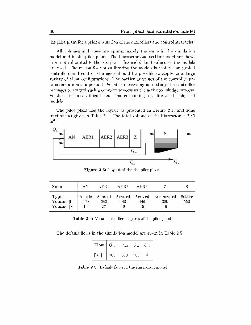
The pilot plant has the layout as presented in Figure 2.3, and zonefractions as given in Table 2.4. The total volume of the bioreactor is 2.35m3.
AER1 AER2 AER3AN ZS
Q
Q
Q Q
in
int
sl w
Figure 2.3: Layout of the the pilot plant.
Zone AN AER1 AER2 AER3 Z S
Type Anoxic Aerated Aerated Aerated Non-aerated SettlerVolume [l] 460 630 440 440 380 550Volume [%] 19 27 19 19 16
Table 2.4: Volume of di�erent parts of the pilot plant
The default ows in the simulation model are given in Table 2.5.
Flow Qin Qint Qsl Qw
[l/h] 200 600 200 4
Table 2.5: Default ows in the simulation model

2.3 The simulation model 31
2.3.2 The bioreactor model
The bioreactor model describes removal of organic matter, nitri�cation,and denitri�cation. The bioreactor model is simulated with IAWQ modelpresented by Henze et al. (1987) with the following exceptions:
� SI (inert soluble organic matter) and SALK (total alkalinity) are notincluded, since they are not needed in this study.
� The inert (XI;IAWQ) and particulate (XP;IAWQ) matter are combinedinto one variable since their di�erent fractions are not interesting inthis study. Hence let XI = XI;IAWQ +XP;IAWQ.
� A term to describe the oxygen transfer has been added in the equationfor the dissolved oxygen (SO). It is KLa(u)(SO;sat�SO), where KLais the oxygen transfer function, u is the air ow rate, and SO;sat is thesaturated dissolved oxygen concentration.
This is the same model as is implemented in Simnon (Elmqvist et al.
1986) by Wikstr�om (1993), but is slightly modi�ed for the use in Regsim
(Gustafsson 1988). Another settler model is also implemented, see Section2.3.4.
2.3.3 Di�erential equations and parameter values
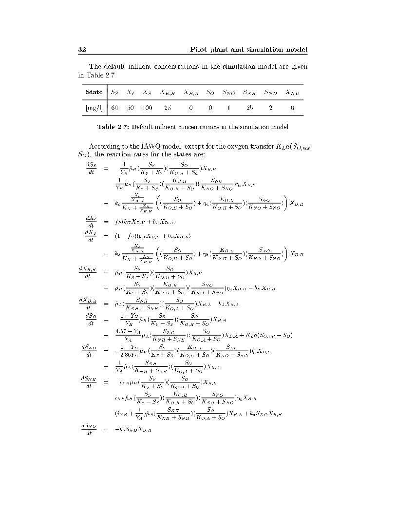
The reaction rates for the states are in Table 2.6 are presented here.
SNH(t) soluble ammonium nitrogenSNO(t) soluble nitrate nitrogenSND(t) soluble biodegradable organic nitrogenSO(t) dissolved oxygenSS(t) soluble substrateXB;A(t) autotrophic biomassXB;H(t) heterotrophic biomassXND(t) particulate biodegradable organic nitrogenXS(t) slowly biodegradable substrateXI(t) particulate matter & products
Table 2.6: States included in the model.
The states starting with an X are particulate and the ones with a S aresoluble.
32 Pilot plant and simulation model
The default in uent concentrations in the simulation model are givenin Table 2.7.
State SS XI XS XB;H XB;A SO SNO SNH SND XND
[mg/l] 60 50 100 25 0 0 1 25 2 6
Table 2.7: Default in uent concentrations in the simulation model
According to the IAWQmodel, except for the oxygen transferKLa(SO;sat�SO), the reaction rates for the states are:
dSS
dt= �
1
YH�H(
SS
KS + SS)(
SO
KO;H + SO)XB;H
�1
YH�H(
SS
KS + SS)(
KO;H
KO;H + SO)(
SNO
KNO + SNO)�gXB;H
+ kh
XSXB;H
KX + XSXB;H
�(
SO
KO;H + SO) + �h(
KO;H
KO;H + SO)(
SNO
KNO + SNO)
�XB;H
dXI
dt= fP (bHXB;H + bAXB;A)
dXS
dt= (1� fP )(bHXB;H + bAXB;A)
� kh
XSXB;H
KX + XSXB;H
�(
SO
KO;H + SO) + �h(
KO;H
KO;H + SO)(
SNO
KNO + SNO)
�XB;H
dXB;H
dt= �H(
SS
KS + SS)(
SO
KO;H + SO)XB;H
+ �H(SS
KS + SS)(
KO;H
KO;H + SO)(
SNO
KNO + SNO)�gXB;H � bHXB;H
dXB;A
dt= �A(
SNH
KNH + SNH)(
SO
KO;A + SO)XB;A � bAXB;A
dSO
dt= �
1� YH
YH�H(
SS
KS + SS)(
SO
KO;H + SO)XB;H
�4:57 � YA
YA�A(
SNH
KNH + SNH)(
SO
KO;A + SO)XB;A +KLa(SO;sat � SO)
dSNO
dt= �
1� YH
2:86YH�H(
SS
KS + SS)(
KO;H
KO;H + SO)(
SNO
KNO + SNO)�gXB;H
+1
YA�A(
SNH
KNH + SNH)(
SO
KO;A + SO)XB;A
dSNH
dt= �iXB�H(
SS
KS + SS)(
SO
KO;H + SO)XB;H
� iXB �H(SS
KS + SS)(
KO;H
KO;H + SO)(
SNO
KNO + SNO)�gXB;H
� (iXB +1
YA)�A(
SNH
KNH + SNH)(
SO
KO;A + SO)XB;A + kaSNDXB;H
dSND
dt= �kaSNDXB;H

2.3 The simulation model 33
+XND
XS
kh
XSXB;H
KX + XSXB;H
�(
SO
KO;H + SO) + �h(
KO;H
KO;H + SO)(
SNO
KNO + SNO)
�XB;H
dXND
dt= (iXB � fP iXP )(bHXB;H + bAXB;A)
�XND
XSkh
XSXB;H
KX + XSXB;H
�(
SO
KO;H + SO) + �h(
KO;H
KO;H + SO)(
SNO
KNO + SNO)
�XB;H
where the parameter values are given in Table 2.8, which are the defaultvalues reported in Henze et al. (1987) for a temperature of 20oC. Some ofthese parameters show little variation from wastewater to wastewater andmay be considered as constants, but others have larger variations. Thevalues given in Table 2.8 are considered typical for neutral pH and domesticwastewater, but many paramters are strongly in uenced by environmentalconditions, see Henze et al. (1987).
To obtain the complete di�erential equations for the di�erent states, thepreviously given reaction rates have to be complemented with the terms forthe mass balance:
D(t)Zin �D(t)Z
where Zin(t) is the in uent concentration, Z(t) is the e�uent concentrationwhich is equal to the concentration in the zone if the zone is completelymixed, D(t) is the dilution rate ( ow/volume).
To give more understanding of the di�erent di�erential equations whichdescribes the reaction rates for the states, some comments for a couple ofthe equations are given (taken from Jeppsson (1996)).
� The change in heterotrophic biomass (XB;H) depends on three pro-cesses: Aerobic growth (the term which is multiplied by SO), anoxicgrowth (the term which is multiplied by SNO), and decay.
� The change in autotrophic biomass (XB;A) is similar to the changein XB;H , but there is no growth in an anoxic environment.
� The soluble substrate (SS) concentration is reduced by the growth ofheterotrophic bacteria (XB;H) and increased by hydrolysis.
� The ammonium concentration (SNH) is a�ected by the growth ofboth XB;H and XB;A, since ammonium is used as a nitrogen sourcein the cell mass. The nitri�cation process also reduce the ammoniumconcentration.
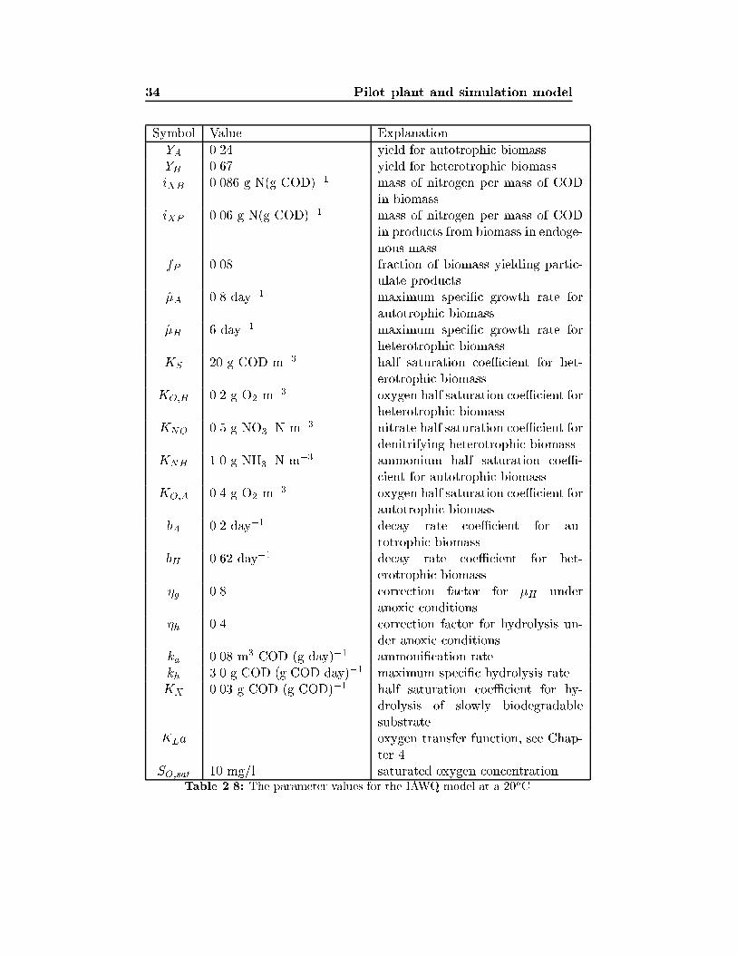
34 Pilot plant and simulation model
Symbol Value Explanation
YA 0.24 yield for autotrophic biomassYH 0.67 yield for heterotrophic biomassiXB 0.086 g N(g COD)�1 mass of nitrogen per mass of COD
in biomassiXP 0.06 g N(g COD)�1 mass of nitrogen per mass of COD
in products from biomass in endoge-nous mass
fP 0.08 fraction of biomass yielding partic-ulate products
�A 0.8 day�1 maximum speci�c growth rate forautotrophic biomass
�H 6 day�1 maximum speci�c growth rate forheterotrophic biomass
KS 20 g COD m�3 half saturation coe�cient for het-erotrophic biomass
KO;H 0.2 g O2 m�3 oxygen half saturation coe�cient for
heterotrophic biomassKNO 0.5 g NO3�N m�3 nitrate half saturation coe�cient for
denitrifying heterotrophic biomassKNH 1.0 g NH3�N m�3 ammonium half saturation coe�-
cient for autotrophic biomassKO;A 0.4 g O2 m
�3 oxygen half saturation coe�cient forautotrophic biomass
bA 0.2 day�1 decay rate coe�cient for au-totrophic biomass.
bH 0.62 day�1 decay rate coe�cient for het-erotrophic biomass
�g 0.8 correction factor for �H underanoxic conditions
�h 0.4 correction factor for hydrolysis un-der anoxic conditions
ka 0.08 m3 COD (g day)�1 ammoni�cation ratekh 3.0 g COD (g COD day)�1 maximum speci�c hydrolysis rateKX 0.03 g COD (g COD)�1 half saturation coe�cient for hy-
drolysis of slowly biodegradablesubstrate
KLa oxygen transfer function, see Chap-ter 4
SO;sat 10 mg/l saturated oxygen concentrationTable 2.8: The parameter values for the IAWQ model at a 20oC.
2.3 The simulation model 35
� The nitrate concentration (SNO) is increased by nitri�cation, anddecreased by denitri�cation.
2.3.4 The settler model
The settler is an important part of the activated sludge process. It is usedfor two purposes: clari�cation and thickening. In a settler, particulatematter in the water from the bioreactor sink to the bottom of the settler(thickening), and clear water is produced (clari�cation) and removed inthe top of the settler. The particulate matter at the bottom of the settler(the activated sludge) contains necessary microorganisms for the biologicalreactions. The sludge is recirculated to the bioreactor to maintain a desiredsolids level.
There exist many di�erent settler models in the literature. Grijspeerdtet al. (1995) have, however, made a comparative study where they foundthat the model by Tak�acs et al. (1991) gave the most reliable results.
Jeppsson (1996) points out that in the traditional layer models, the uxes are de�ned by empirical reasoning and sometimes contain ad hoc
assumptions. The solution will then depend on the number of layers andthere is no guarantee that the model produces physically relevant solutionssatisfying the continuity equation. Despite the important fact as Jeppsson(1996) points out, the model by Tak�acs et al. (1991) will be used since itstill provides a good description of the real behavior.
The settler model by Tak�acs et al. (1991) is used with two extensions:
� Soluble matters are included, and described by the following model:
dS
dt=Q
V(Sin � S)
where S represent any soluble state in Table 2.6.
� The composition of the suspended material is considered, and ishence not treated as a whole MLVSS (mixed liquor volatile suspendedsolids). That is, XI , XS , XBA, XBH , and XND are calculated in eachlayer. Example: XI is calculated in the bottom layer according to
dXI;n
dt=
1
h
�(Qs +Qw)
A(XI;n�1 �XI;n) + min(vs;n�1XI;n�1; vs;nXI;n)
�
The settler is modeled as a tank with several horizontal layers whereeach layer is assumed to be completely mixed, see Figure 2.4.
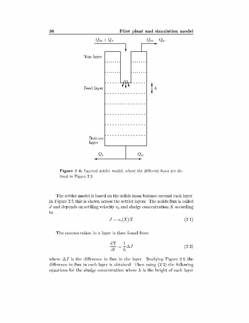
36 Pilot plant and simulation model
?
-
� -
6?
?�� BBN
Qin �Qw
QwQs
Qin +Qs
Top layer
Feed layer
Bottomlayer
h
Figure 2.4: Layered settler model, where the di�erent ows are de-
�ned in Figure 2.3.
The settler model is based on the solids mass balance around each layer.In Figure 2.5 this is shown across the settler layers. The solids ux is calledJ and depends on settling velocity vs and sludge concentration X accordingto
J = vs(X)X (2.1)
The concentration in a layer is then found from
dX
dt=
1
h�J (2.2)
where �J is the di�erence in ux in the layer. Studying Figure 2.5 thedi�erence in ux in each layer is obtained. Then using (2.2) the followingequations for the sludge concentration where h is the height of each layer
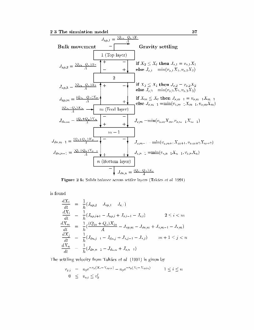
2.3 The simulation model 37
Gravity settlingBulk movement
1 (Top layer)
2
m (Feed layer)
m+ 1
n (Bottom layer)
6
?
??
? ?
??
6
6
-
?
?
?-
if X2 � Xt then Js;1 = vs;1X1
else Js;1 =min(vs;1X1; vs;2X2)
if X3 � Xt then Js;2 = vs;2X2
else Js;2 =min(vs;2X2; vs;3X3)
if Xm � Xt then Js;m�1 = vs;m�1Xm�1
else Js;m�1 =min(vs;m�1Xm�1; vs;mXm)
Js;m =min(vs;mXm; vs;m+1Xm+1)
Js;m+1 =min(vs;m+1Xm+1; vs;m+2Xm+2)
Js;n�1 =min(vs;n�1Xn�1; vs;nXn)
Jup;2 =(Qin�Qw)X2
A
Jup;3 =(Qin�Qw)X3
A
Jup;m = (Qin�Qw)Xm
A
Jdn;m = (Qs+Qw)Xm
A
Jdn;m+1 =(Qs+Qw)Xm+1
A
Jdn;n�1 =(Qs+Qw)Xn�1
A
+
+
+
+
+ +
++
��
�
�
� �
� �
�
�Jup;1 =
(Qin�Qw)X1
A
(Qin+Qs)Xin
A
Jdn;n =(Qs+Qw)Xn
A
Figure 2.5: Solids balance across settler layers (Tak�acs et al. 1991).
is found.
dX1
dt=
1
h(Jup;2 � Jup;1 � Js;1)
dXi
dt=
1
h(Jup;i+1 � Jup;i + Js;i�1 � Js;i) 2 � i < m
dXm
dt=
1
h((Qin +Qs)Xin
A� Jup;m � Jdn;m + Js;m�1 � Js;m)
dXj
dt=
1
h(Jdn;j�1 � Jdn;j + Js;j�1 � Js;j) m+ 1 � j < n
dXn
dt=
1
h(Jdn;n�1 � Jdn;n + Js;n�1)
The settling velocity from Tak�acs et al. (1991) is given by
vs;i = v0e�rh(Xi�Xmin) � v0e
�rp(Xi�Xmin) 1 � i � n
0 � vs;i � v00
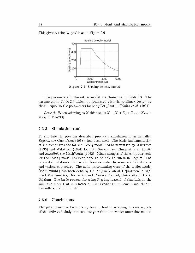
38 Pilot plant and simulation model
This gives a velocity pro�le as in Figure 2.6.
0 2000 4000 60000
100
200
300
400
Concentration (X)
Set
tling
vel
ocity
(vs
)
Settling velocity model
Figure 2.6: Settling velocity model.
The parameters in the settler model are chosen as in Table 2.9. Theparameters in Table 2.9 which are connected with the settling velocity arechosen equal to the parameters for the pilot plant in Tak�acs et al. (1991).
Remark: When referring to X this means X = XI+XS+XBA+XBH+XND (=MLVSS).
2.3.5 Simulation tool
To simulate the previous described process a simulation program calledRegsim, see Gustafsson (1988), has been used. The basic implementationof the computer code for the IAWQ model has been written by Wikstr�om(1993) and Wikstr�om (1994) for both Simnon, see Elmqvist et al. (1986)and Simulink, see MathWorks (1992). Minor changes of the computer codefor the IAWQ model has been done to be able to run it in Regsim. Theoriginal simulation code has also been extended by some additional zonesand various controllers. The main programming work of the settler model(for Simulink) has been done by Dr. Zhiguo Yuan at Department of Ap-plied Mathematics, Biometrics and Process Control, University of Gent,Belgium. The basic reasons for using Regsim, instead of Simulink, in thesimulations are that it is faster and it is easier to implement models andcontrollers than in Simulink.
2.3.6 Conclusions
The pilot plant has been a very fruitful tool in studying various aspectsof the activated sludge process, ranging from innovative operating modes,
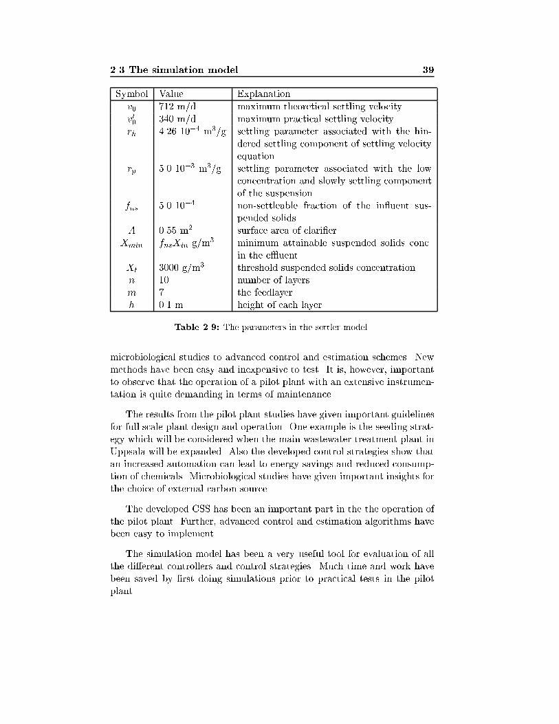
2.3 The simulation model 39
Symbol Value Explanation
v0 712 m/d maximum theoretical settling velocity.v00 340 m/d maximum practical settling velocity.rh 4.26 10�4 m3/g settling parameter associated with the hin-
dered settling component of settling velocityequation.
rp 5.0 10�3 m3/g settling parameter associated with the lowconcentration and slowly settling componentof the suspension.
fns 5.0 10�4 non-settleable fraction of the in uent sus-pended solids.
A 0.55 m2 surface area of clari�er.Xmin fnsXin g/m3 minimum attainable suspended solids conc.
in the e�uent.Xt 3000 g/m3 threshold suspended solids concentration.n 10 number of layers.m 7 the feedlayer.h 0.1 m height of each layer.
Table 2.9: The parameters in the settler model.
microbiological studies to advanced control and estimation schemes. Newmethods have been easy and inexpensive to test. It is, however, importantto observe that the operation of a pilot plant with an extensive instrumen-tation is quite demanding in terms of maintenance.
The results from the pilot plant studies have given important guidelinesfor full scale plant design and operation. One example is the seeding strat-egy which will be considered when the main wastewater treatment plant inUppsala will be expanded. Also the developed control strategies show thatan increased automation can lead to energy savings and reduced consump-tion of chemicals. Microbiological studies have given important insights forthe choice of external carbon source.
The developed CSS has been an important part in the the operation ofthe pilot plant. Further, advanced control and estimation algorithms havebeen easy to implement.
The simulation model has been a very useful tool for evaluation of allthe di�erent controllers and control strategies. Much time and work havebeen saved by �rst doing simulations prior to practical tests in the pilotplant.

40 Pilot plant and simulation model
Chapter 3
Control of external carbon
ow rate in a
pre-denitrifying activated
sludge process
Biological nitrogen removal in activated sludge processes is dependent onsu�cient supplies of easily metabolized carbon compounds for the denitrify-ing bacterial population. An external carbon source can increase denitri�-cation rates and compensate for de�ciencies in the in uent carbon/nitrogenratio. This works, however, only if the denitri�cation process is carbonconstrained. Possible carbon sources include methanol, ethanol, acetate,primary sludge and various industrial waste products. In this chapter somedi�erent controllers and control strategies for the external carbon sourcedosage in a pre-denitrifying activated sludge process are suggested.
It is important to control the ow rate of the external carbon source.A too low dosage will leave the denitri�cation process carbon constrainedand the full capacity for nitrogen removal is not used. A too high carbondosage is expensive, may cause carbon spill and increases the sludge pro-duction which a�ects the nitri�cation capacity, see Aspegren et al. (1992)and Hellstr�om and Bosander (1990). Another problem with overdosing,discussed in Hallin and Pell (1996), is that the microorganisms may losetheir capacity to use natural existing carbon sources.
When adding an external carbon source one should be aware that avery selected microbial system may be induced, and it may take weeks for
42 Control of external carbon ow rate
the microorganisms to adapt to the external carbon. It has been arguedby Nyberg et al. (1993) and Andersson et al. (1995) that the ow rateof external carbon source should not be controlled automatically, due tothe obtained sensitive microbial system, reliability problems with on-linesensors, and because the e�uent standard of nitrate is based on averagevalues. To sustain the adapted microbial system, which can metabolizeexternal carbon, the external carbon ow rate should never be switchedo�. It is easy to design a controller which never give a carbon ow ratebelow a pre-speci�ed minimum ow rate. Note also that it is possible toswitch o� some carbon sources for several days (e.g. ethanol) without losingdenitri�cation capacity, see Hasselblad and Hallin (1996). Further, thereliability problems with the on-line sensors can be reduced by maintainingthese frequently. It is also likely that on-line nitrate sensors will be morereliable in the future. According to e.g. Lynggaard-Jensen et al. (1996)reliable sensors already exist.
A constant ow rate of carbon is only advantageous when the in uentvariations of the carbon/nitrogen ratio are small. When the variations arelarge, a constant carbon dosage will be too low during some hours and toohigh during other periods. The average nitrate concentration will then notbe reduced as much with a constant dosage as it would with a controlleddosage. In a typical plant the load often varies by a factor of 6 or more,see Van Impe et al. (1992). If external carbon is added in the last step of awastewater treatment plant, it is very important to give a correct dosage,since there are no later steps in the plant where an excessive dosage canbe degraded. An example is control of the nitrate concentration in a sand�lter, see Hultman et al. (1994).
A reasonable control strategy for the carbon dosage is to keep the nitratelevel in the anoxic zone (just before the aerobic zone in a pre-denitrifyingplant) at a constant low level. That strategy has been discussed in Hell-str�om and Bosander (1990). An approach where the controller design isbased on the IAWQ model has been done by Yuan et al. (1996). Anotherstrategy where the carbon dosage is based on presence or no presence ofnitrate in the e�uent has been suggested by Vanrolleghem et al. (1993).The carbon dosage has been controlled by considering the oxygen demandin Linde (1993). Brenner (1991) presented a simulation study with anexternal carbon source and found that the aerobic volume fraction andrecirculation rate should be increased when carbon is added, but the aero-bic volume fraction could be decreased if the biomass instead is increased.Londong (1992) has also controlled the nitrate level, but the interest wasmainly focused on the recirculation rate instead of the carbon dosage. Therecirculation rate has also been considered in Andersson et al. (1995). The
3.1 Modeling the nitrate process 43
carbon dosage control in an alternating nitri�cation-denitri�cation processis di�erent compared to the continuous activated sludge plant. In thatprocess, the nitrate level is not used for control. Instead a model of thedenitri�cation rate is estimated, which is then used to determine the carbondosage, so that the denitri�cation is completed within the current operationcycle, see e.g. Isaacs et al. (1993).
The carbon dosage controllers presented here can all use feedforwardfrom in uent mass ow of Total Organic Carbon (TOC) and mass ow ofnitrate in recirculated water. Instead of using feedforward from recirculatednitrate, in uent ammonium may be used, but the recirculated nitrate moredirectly in uences the nitrate level in the anoxic zone. Flow changes inthe internal recirculation will also make that feedforward more unreliable,hence feedforward from the nitrate concentration is preferred.
The outline of the chapter is as follows. In Section 3.1 the model of thenitrate process is discussed. The di�erential equation for the nitrate con-centration is studied further and an ARX approximation is presented. Thecontrol strategy is outlined in Section 3.2. Signals suitable for feedforward,and di�erent types of controllers are also discussed. The following four dif-ferent controllers are evaluated: a PID-controller with �xed parameters inSection 3.3, a model-based adaptive PID controller in Section 3.4, a directadaptive controller in Section 3.5, and an indirect adaptive controller inSection 3.6. Some practical aspect for adaptive control are considered inSection 3.7. Simulations using the four di�erent controllers are presentedin Section 3.8. The direct adaptive controller is also evaluated at the pilotplant; the experiment is presented in Section 3.9. Finally, conclusions aregiven in Section 3.10.
3.1 Modeling the nitrate process
To design a controller with high performance, some kind of process modelis usually needed. The IAWQ model is rather complex, since it involves 13nonlinear coupled di�erential equations, and several more or less unknownparameters, which are di�cult to estimate on-line, see e.g., Jeppsson (1993).The complete IAWQ model is not suitable for controller design, parts of itmay, however, be useful. This has been used in the design by Yuan et al.
(1996) together with the assumption that there are only small variationsin the parameters of the IAWQ. To illustrate some of the problems in thedynamics of the nitrate concentration, its di�erential equation based on theIAWQ model is studied. Assuming zero dissolved oxygen concentration,which is reasonable for an anoxic zone, the following di�erential equation
44 Control of external carbon ow rate
for the soluble nitrate SNO(t) is obtained.
dSNO
dt= DinSNOin�DoutSNO�1� YH
2:86YH�H(
SSKS + SS
)(SNO
KNO + SNO
)�gXB;H
(3.1)where
SNO(t) is the soluble nitrateSNOin(t) is the in uent soluble nitrateSS(t) is the soluble substrate. The external carbon is included in SSXB;H(t) is the heterotrophic biomassDin(t) is the in uent dilution rate ( ow/volume)Dout(t) is the e�uent dilution rateYH is the yield for heterotrophic biomass = 0.67�H is the maximum speci�c growth rate for heterotrophic biomass
= 0.25 (=6/24) h�1 at 20o CKS is the half saturation coe�cient for heterotrophic biomass
= 20 g COD m�3
KNO is the nitrate half saturation coe�cient for denitrifyingheterotrophic biomass = 0.5 g NO3� N m�3
�g is the correction factor for �H under anoxic conditions = 0.8
The parameters in (3.1) are not constant. They vary with, e.g., waste-water composition, temperature, and heterotrophic biomass which usuallyis not measurable. The values given above are the default values at 20o Cin Henze et al. (1987).
As can be seen in equation (3.1) the gain of the process varies with theSS, SNO, and XB;H . It also depends on time varying parameters as KS
and KNO, and ow rates. Since there are so many uncertainties in theprocess, we prefer to estimate an ARX model, which is easier to estimatethan all the model parameters in (3.1). An ARX model is also easier touse in a controller design. An approach to estimate a model where some ofthe physical knowlegde in (3.1) is used will, however, also be utilized. Byusing real-time estimation (estimation for time-varying systems) the linearmodel can be adapted to time-varying operating points. If the parametervariations in the estimated linear model are large it may be suitable to usean adaptive controller, but if the estimated model is almost time-invariantit is better to use a non-adaptive controller.
The following ARX model will be used to model the nitrate process
A(q�1)y(t) = B(q�1)q�ku(t)+D1(q�1)q�d1w1(t)+D2(q
�1)q�d2w2(t)+n(t)(3.2)
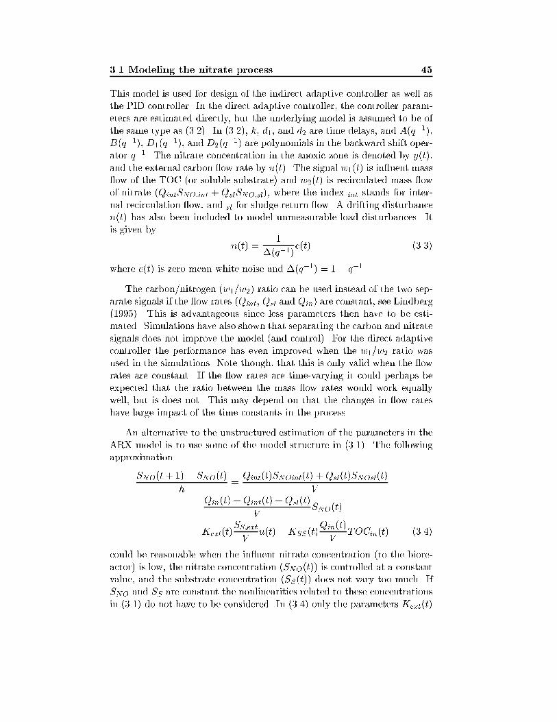
3.1 Modeling the nitrate process 45
This model is used for design of the indirect adaptive controller as well asthe PID controller. In the direct adaptive controller, the controller param-eters are estimated directly, but the underlying model is assumed to be ofthe same type as (3.2). In (3.2), k, d1, and d2 are time delays, and A(q
�1),B(q�1), D1(q
�1), and D2(q�1) are polynomials in the backward shift oper-
ator q�1. The nitrate concentration in the anoxic zone is denoted by y(t),and the external carbon ow rate by u(t). The signal w1(t) is in uent mass ow of the TOC (or soluble substrate) and w2(t) is recirculated mass owof nitrate (QintSNO;int + QslSNO;sl), where the index int stands for inter-nal recirculation ow, and sl for sludge return ow. A drifting disturbancen(t) has also been included to model unmeasurable load disturbances. Itis given by
n(t) =1
�(q�1)e(t) (3.3)
where e(t) is zero mean white noise and �(q�1) = 1� q�1.
The carbon/nitrogen (w1=w2) ratio can be used instead of the two sep-arate signals if the ow rates (Qint, Qsl and Qin) are constant, see Lindberg(1995). This is advantageous since less parameters then have to be esti-mated. Simulations have also shown that separating the carbon and nitratesignals does not improve the model (and control). For the direct adaptivecontroller the performance has even improved when the w1=w2 ratio wasused in the simulations. Note though, that this is only valid when the owrates are constant. If the ow rates are time-varying it could perhaps beexpected that the ratio between the mass ow rates would work equallywell, but is does not. This may depend on that the changes in ow rateshave large impact of the time constants in the process.
An alternative to the unstructured estimation of the parameters in theARX model is to use some of the model structure in (3.1). The followingapproximation
SNO(t+ 1)� SNO(t)
h=Qint(t)SNOint(t) +Qsl(t)SNOsl(t)
V
�Qin(t) +Qint(t) +Qsl(t)
VSNO(t)
�Kext(t)SS;extV
u(t)�KSS(t)Qin(t)
VTOCin(t) (3.4)
could be reasonable when the in uent nitrate concentration (to the biore-actor) is low, the nitrate concentration (SNO(t)) is controlled at a constantvalue, and the substrate concentration (SS(t)) does not vary too much. IfSNO and SS are constant the nonlinearities related to these concentrationsin (3.1) do not have to be considered. In (3.4) only the parameters Kext(t)
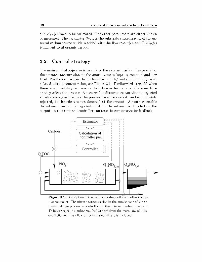
46 Control of external carbon ow rate
and KSS(t) have to be estimated. The other parameters are either knownor measured. The parameter SS;ext is the substrate concentration of the ex-ternal carbon source which is added with the ow rate u(t), and TOCin(t)is in uent total organic carbon.
3.2 Control strategy
The main control objective is to control the external carbon dosage so thatthe nitrate concentration in the anoxic zone is kept at constant and lowlevel. Feedforward is used from the in uent TOC and the internally recir-culated nitrate concentration, see Figure 3.1. Feedforward is useful whenthere is a possibility to measure disturbances before or at the same timeas they a�ect the process. A measurable disturbance can then be rejectedsimultaneously as it enters the process. In some cases it can be completelyrejected, i.e. its e�ect is not detected at the output. A non-measurabledisturbance can not be rejected until the disturbance is detected on theoutput, at this time the controller can start to compensate by feedback.
Estimator
Controller
controller par.Calculation of
NO3
Carbon
Q NO3,slsl
Q TOC
Q NO3,intint
in
Figure 3.1: Description of the control strategy with an indirect adap-
tive controller. The nitrate concentration in the anoxic zone of the ac-
tivated sludge process is controlled by the external carbon ow rate.
To better reject disturbances, feedforward from the mass ow of in u-
ent TOC and mass ow of recirculated nitrate is included.
3.2 Control strategy 47
In the controller design, it is assumed that the measured TOC levelin the in uent water is correlated with the in uent soluble substrate (SS).The external carbon source is also treated as soluble substrate. Note thatthis assumption makes the model valid only for a process where the sludgehas adapted to the external carbon source. When using a carbon sourcewhere the microorganisms need long time to adapt, e.g. methanol, it isprobably necessary to extend the IAWQ model with an extra substratestate to be able to model the slow adaptation phase of the external carbonto the process. This is a topic for future research.
When no sensors for feedforward measurements are available, one couldconsider the possibility to model the daily variations in in uent concentra-tions and use the predicted disturbances in a feedforward controller. Thistype of feedforward from a knowledge database is also a topic for futureresearch.
Four di�erent carbon dosage controllers will be presented. A PID-controller, a direct adaptive, an indirect adaptive controller, and a model-based adaptive PID controller are studied. In the direct adaptive controllerthe controller parameters are estimated directly, the block calculation of
controller parameters in Figure 3.1 is hence not needed for this controller.The indirect adaptive controller is based on a recursively estimated pro-cess model, which is used for controller design, see Figure 3.1. The fourcontrollers are evaluated on the simulation model of the activated sludgeprocess which was presented in Section 2.3. The direct adaptive controllerhas also been tested at the pilot plant at Kungs�angsverket, Uppsala.
The con�guration of the activated sludge process and sensor placementused in all simulations is shown in Figure 3.1. The activated sludge processhence consists of �ve zones and a settler. The external carbon is added inthe �rst zone, which is anoxic. The nitrate concentration is also measuredin that zone. The following three zones are aerobic, where the dissolvedoxygen is controlled at a certain prespeci�ed level. The last zone is non-aerated, in order to reduce the dissolved oxygen (DO) concentration in therecirculated water to improve denitri�cation. In all the recirculated water(internal rec. and sludge rec.) the nitrate concentration is measured. Thenitrate concentration in the in uent water is so small that it is no pointto use feedforward from that ow. The TOC concentration in the in uentwastewater is, however, measured. If the mass ow variations of nitrate inthe recirculated sludge are small, feedforward from this variation does notgive any performance improvement, and this sensor is hence not necessary.
48 Control of external carbon ow rate
3.3 A PID-controller
The PID controller is probably the most widely used controller. Well tunedit can give reasonable performance for many processes. It is, however, di�-cult to tune a PID controller manually, especially if the process dynamics isslow. There exist di�erent ways to tune a PID controller. For example, theclassical Ziegler-Nichols rules can be used, but they give fairly low damping.Often, a better choice is auto-tuning which is based on the relay method,see �Astr�om and H�agglund (1984). Auto-tuning works as follows, the con-troller is disconnected and replaced by a relay, which induces a limit cycleoscillation. The period and the amplitude of the oscillations give a pointon the Nyquist curve, which is used to choose the controller parameters.This method of tuning can also be applied to other controller structuresthan PID-controllers.
Another way to obtain the controller parameters is to identify a modelof the system using a system identi�cation algorithm, for example, a leastsquares method or a prediction error method, see e.g. S�oderstr�om and Sto-ica (1989). The identi�ed model is then used to derive the controller pa-rameters for a desired closed loop response. A problem with this methodis that the closed loop poles can only be chosen arbitrary for a limited setof model structures.
An approach to derive the feedforward is to estimate a model of theprocess and use it together with the feedback (the PID-controller) to derivean optimal (in LQ sense) feedforward. Another simpler approach is just toapply a static gain from the feedforward measurements. In the simulationsin Section 3.8 such an approach is used.
The PID-controller with feedforward has the following structure.
�u(t) = K[(e(t)� e(t� 1)) +h
Tie(t) � TD
h(yf (t)� 2yf (t� 1) + yf (t� 2))]
+ Kf1�w1(t) +Kf2�w2(t) (3.5)
u(t) = u(t� 1) + �u(t) (3.6)
e(t) = yref (t)� y(t) (3.7)
yf (t) = pyf (t� 1) + (1� p)y(t) (3.8)
where K, Ti TD are the usual PID parameters, h is the sampling interval,Kf1 and Kf2 are the feedforward gains, yf (t) is y(t) low-pass �ltered and�w1(t) and �w2(t) are the di�erentiated (�w1(t) = w1(t) � w1(t � 1))feedforward signals, i.e. in uent mass ow of the TOC, and recirculatedmass ow of nitrate. In (3.5), the derivative of the error e(t) is not used,instead only the derivative of yf (t) is used to avoid large changes in the
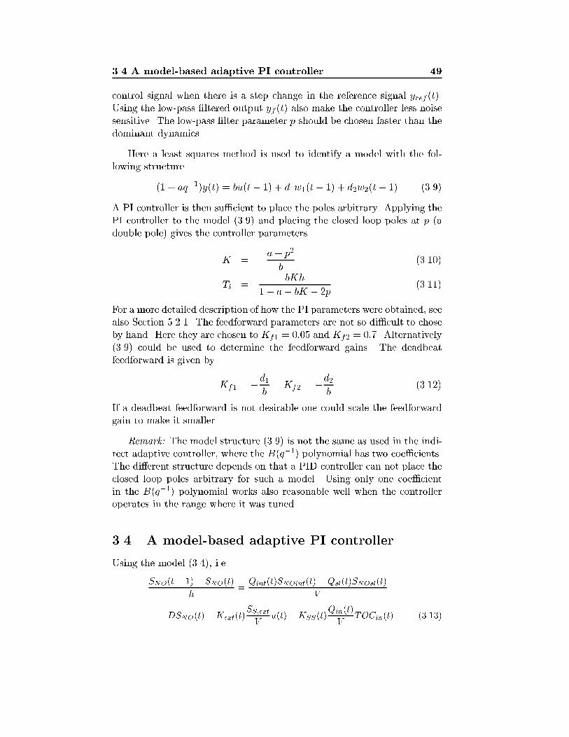
3.4 A model-based adaptive PI controller 49
control signal when there is a step change in the reference signal yref (t).Using the low-pass �ltered output yf (t) also make the controller less noisesensitive. The low-pass �lter parameter p should be chosen faster than thedominant dynamics.
Here a least squares method is used to identify a model with the fol-lowing structure
(1 + aq�1)y(t) = bu(t� 1) + d1w1(t� 1) + d2w2(t� 1) (3.9)
A PI controller is then su�cient to place the poles arbitrary. Applying thePI controller to the model (3.9) and placing the closed loop poles at p (adouble pole) gives the controller parameters
K = �a+ p2
b(3.10)
Ti =bKh
1� a� bK � 2p(3.11)
For a more detailed description of how the PI parameters were obtained, seealso Section 5.2.1. The feedforward parameters are not so di�cult to choseby hand. Here they are chosen to Kf1 = 0:05 and Kf2 = 0:7. Alternatively(3.9) could be used to determine the feedforward gains. The deadbeatfeedforward is given by
Kf1 = �d1b
Kf2 = �d2b
(3.12)
If a deadbeat feedforward is not desirable one could scale the feedforwardgain to make it smaller.
Remark: The model structure (3.9) is not the same as used in the indi-rect adaptive controller, where the B(q�1) polynomial has two coe�cients.The di�erent structure depends on that a PID controller can not place theclosed loop poles arbitrary for such a model. Using only one coe�cientin the B(q�1) polynomial works also reasonable well when the controlleroperates in the range where it was tuned.
3.4 A model-based adaptive PI controller
Using the model (3.4), i.e.
SNO(t+ 1)� SNO(t)
h=Qint(t)SNOint(t) +Qsl(t)SNOsl(t)
V
�DSNO(t)�Kext(t)SS;ext
Vu(t)�KSS(t)
Qin(t)
VTOCin(t) (3.13)
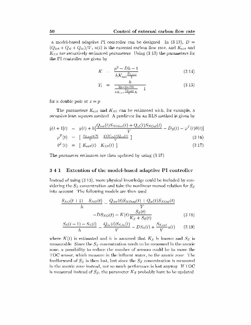
50 Control of external carbon ow rate
a model-based adaptive PI controller can be designed. In (3.13), D =(Qint +Qsl +Qin)=V , u(t) is the external carbon ow rate, and Kext andKSS are recursively estimated parameters. Using (3.13) the parameters forthe PI controller are given by
K =p2 +Dh� 1
hKextSS;extV
(3.14)
Ti =h
2p�2+Dh
hKextSS;extV
K� 1
(3.15)
for a double pole at z = p.
The parameters Kext and KSS can be estimated with, for example, arecursive least squares method. A predictor for an RLS method is given by
y(t+ 1jt) = y(t) + h[Qint(t)SNOint(t) +Qsl(t)SNOsl(t)
V�Dy(t)� 'T (t)�(t)]
'T (t) = [ SS;extu(t)V
TOCin(t)Qin(t)V
] (3.16)
�T (t) = [ Kext(t) KSS(t) ] (3.17)
The parameter estimates are then updated by using (3.57).
3.4.1 Extention of the model-based adaptive PI controller
Instead of using (3.13), more physical knowledge could be included by con-sidering the SS concentration and take the nonlinear monod relation for SSinto account. The following models are then used
SNO(t+ 1)� SNO(t)
h=Qint(t)SNOint(t) +Qsl(t)SNOsl(t)
V
�DSNO(t)�K(t)SS(t)
KS + SS(t)(3.18)
SS(t+ 1)� SS(t)
h=Qin(t)SS;in(t)
V�DSS(t) +
SS;extV
u(t) (3.19)
where K(t) is estimated and it is assumed that KS is known and SS ismeasurable. Since the SS concentration needs to be measured in the anoxiczone, a possibility to reduce the number of sensors could be to move theTOC sensor, which measure in the in uent water, to the anoxic zone. Thefeedforward of SS is then lost, but since the SS concentration is measuredin the anoxic zone instead, not so much performace is lost anyway. If TOCis measured instead of SS, the parameter KS probably have to be updated.
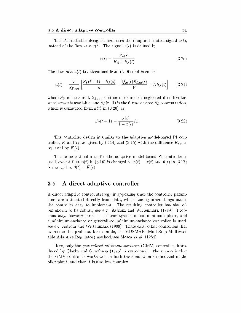
3.5 A direct adaptive controller 51
The PI controller designed here uses the temporal control signal x(t),instead of the ow rate u(t). The signal x(t) is de�ned by
x(t) =SS(t)
KS + SS(t)(3.20)
The ow rate u(t) is determined from (3.19) and becomes
u(t) =V
SS;ext
�SS(t+ 1)� SS(t)
h� Qin(t)SS;in(t)
V+DSS(t)
�(3.21)
where SS is measured, SS;in is either measured or neglected if no feedfor-ward sensor is available, and SS(t+1) is the future desired SS concentration,which is computed from x(t) in (3.20) as
SS(t+ 1) =x(t)
1� x(t)KS (3.22)
The controller design is similar to the adaptive model-based PI con-troller, K and Ti are given by (3.14) and (3.15) with the di�erence Kext isreplaced by K(t).
The same estimator as for the adaptive model-based PI controller isused, except that '(t) in (3.16) is changed to '(t) = x(t) and �(t) in (3.17)is changed to �(t) = K(t).
3.5 A direct adaptive controller
A direct adaptive control strategy is appealing since the controller param-eters are estimated directly from data, which among other things makesthe controller easy to implement. The resulting controller has also of-ten shown to be robust, see e.g. �Astr�om and Wittenmark (1989). Prob-lems may, however, arise if the true system is non-minimum phase, anda minimum-variance or generalized minimum-variance controller is used,see e.g. �Astr�om and Wittenmark (1989). There exist other controllers thatovercome this problem, for example, the MUSMAR (MultiStep Multivari-able Adaptive Regulator) method, see Mosca et al. (1984).
Here, only the generalized minimum-variance (GMV) controller, intro-duced by Clarke and Gawthrop (1975) is considered. The reason is thatthe GMV controller works well in both the simulation studies and in thepilot plant, and that it is also less complex.
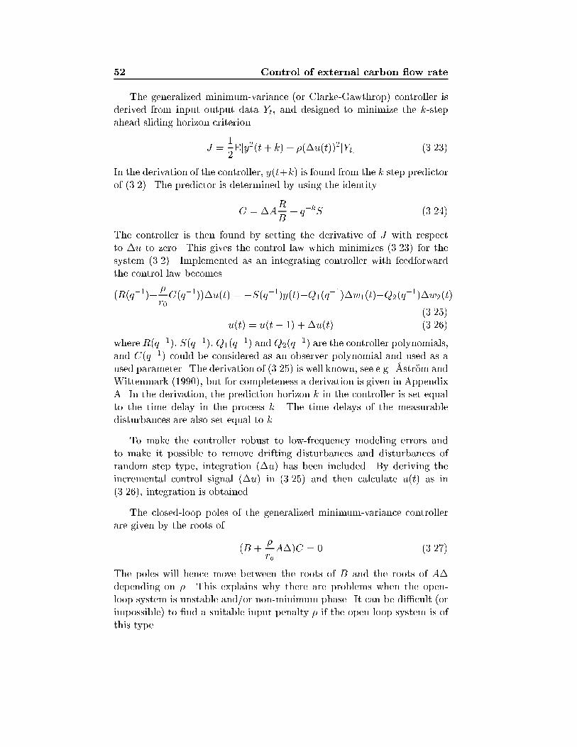
52 Control of external carbon ow rate
The generalized minimum-variance (or Clarke-Gawthrop) controller isderived from input output data Yt, and designed to minimize the k-stepahead sliding horizon criterion
J =1
2E[y2(t+ k) + �(�u(t))2jYt] (3.23)
In the derivation of the controller, y(t+k) is found from the k step predictorof (3.2). The predictor is determined by using the identity
C = �AR
B+ q�kS (3.24)
The controller is then found by setting the derivative of J with respectto �u to zero. This gives the control law which minimizes (3.23) for thesystem (3.2). Implemented as an integrating controller with feedforwardthe control law becomes
(R(q�1)+�
r0C(q�1))�u(t) = �S(q�1)y(t)�Q1(q
�1)�w1(t)�Q2(q�1)�w2(t)
(3.25)u(t) = u(t� 1) + �u(t) (3.26)
where R(q�1), S(q�1), Q1(q�1) and Q2(q
�1) are the controller polynomials,and C(q�1) could be considered as an observer polynomial and used as aused parameter. The derivation of (3.25) is well known, see e.g. �Astr�om andWittenmark (1990), but for completeness a derivation is given in AppendixA. In the derivation, the prediction horizon k in the controller is set equalto the time delay in the process k. The time delays of the measurabledisturbances are also set equal to k.
To make the controller robust to low-frequency modeling errors andto make it possible to remove drifting disturbances and disturbances ofrandom step type, integration (�u) has been included. By deriving theincremental control signal (�u) in (3.25) and then calculate u(t) as in(3.26), integration is obtained.
The closed-loop poles of the generalized minimum-variance controllerare given by the roots of
(B +�
roA�)C = 0 (3.27)
The poles will hence move between the roots of B and the roots of A�depending on �. This explains why there are problems when the open-loop system is unstable and/or non-minimum phase. It can be di�cult (orimpossible) to �nd a suitable input penalty � if the open loop system is ofthis type.
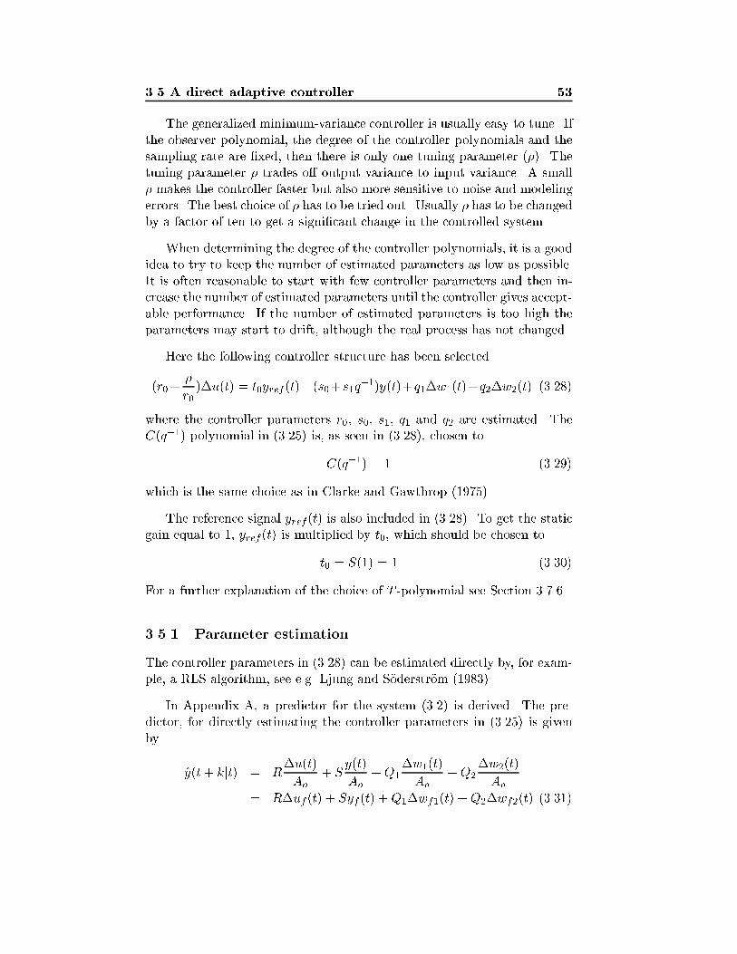
3.5 A direct adaptive controller 53
The generalized minimum-variance controller is usually easy to tune. Ifthe observer polynomial, the degree of the controller polynomials and thesampling rate are �xed, then there is only one tuning parameter (�). Thetuning parameter � trades o� output variance to input variance. A small� makes the controller faster but also more sensitive to noise and modelingerrors. The best choice of � has to be tried out. Usually � has to be changedby a factor of ten to get a signi�cant change in the controlled system.
When determining the degree of the controller polynomials, it is a goodidea to try to keep the number of estimated parameters as low as possible.It is often reasonable to start with few controller parameters and then in-crease the number of estimated parameters until the controller gives accept-able performance. If the number of estimated parameters is too high theparameters may start to drift, although the real process has not changed.
Here the following controller structure has been selected
(r0+�
r0)�u(t) = t0yref(t)�(s0+s1q
�1)y(t)+q1�w1(t)+q2�w2(t) (3.28)
where the controller parameters r0, s0, s1, q1 and q2 are estimated. TheC(q�1) polynomial in (3.25) is, as seen in (3.28), chosen to
C(q�1) = 1 (3.29)
which is the same choice as in Clarke and Gawthrop (1975).
The reference signal yref (t) is also included in (3.28). To get the staticgain equal to 1, yref(t) is multiplied by t0, which should be chosen to
t0 = S(1) = 1 (3.30)
For a further explanation of the choice of T -polynomial see Section 3.7.6.
3.5.1 Parameter estimation
The controller parameters in (3.28) can be estimated directly by, for exam-ple, a RLS algorithm, see e.g. Ljung and S�oderstr�om (1983).
In Appendix A, a predictor for the system (3.2) is derived. The pre-dictor, for directly estimating the controller parameters in (3.25) is givenby
y(t+ kjt) = R�u(t)
Ao
+ Sy(t)
Ao
+Q1�w1(t)
Ao
+Q2�w2(t)
Ao
= R�uf (t) + Syf (t) +Q1�wf1(t) +Q2�wf2(t) (3.31)
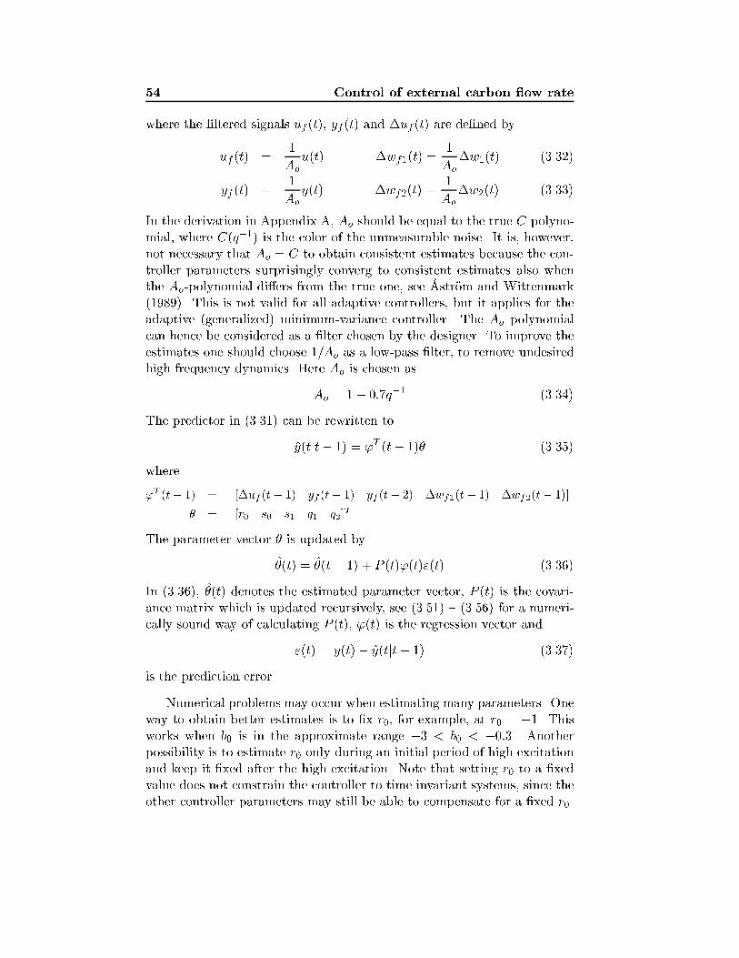
54 Control of external carbon ow rate
where the �ltered signals uf (t), yf (t) and �uf (t) are de�ned by
uf (t) =1
Ao
u(t) �wf1(t) =1
Ao
�w1(t) (3.32)
yf (t) =1
Aoy(t) �wf2(t) =
1
Ao�w2(t) (3.33)
In the derivation in Appendix A, Ao should be equal to the true C polyno-mial, where C(q�1) is the color of the unmeasurable noise. It is, however,not necessary that Ao = C to obtain consistent estimates because the con-troller parameters surprisingly converg to consistent estimates also whenthe Ao-polynomial di�ers from the true one, see �Astr�om and Wittenmark(1989). This is not valid for all adaptive controllers, but it applies for theadaptive (generalized) minimum-variance controller. The Ao polynomialcan hence be considered as a �lter chosen by the designer. To improve theestimates one should choose 1=Ao as a low-pass �lter, to remove undesiredhigh frequency dynamics. Here Ao is chosen as
Ao = 1� 0:7q�1 (3.34)
The predictor in (3.31) can be rewritten to
y(tjt� 1) = 'T (t� 1)� (3.35)
where
'T (t� 1) = [�uf (t� 1) yf (t� 1) yf (t� 2) �wf1(t� 1) �wf2(t� 1)]
� = [r0 s0 s1 q1 q2]T
The parameter vector � is updated by
�(t) = �(t� 1) + P (t)'(t)"(t) (3.36)
In (3.36), �(t) denotes the estimated parameter vector, P (t) is the covari-ance matrix which is updated recursively, see (3.51) { (3.56) for a numeri-cally sound way of calculating P (t), '(t) is the regression vector and
"(t) = y(t)� y(tjt� 1) (3.37)
is the prediction error.
Numerical problems may occur when estimating many parameters. Oneway to obtain better estimates is to �x r0, for example, at r0 = �1. Thisworks when b0 is in the approximate range �3 < b0 < �0:3. Anotherpossibility is to estimate r0 only during an initial period of high excitationand keep it �xed after the high excitation. Note that setting r0 to a �xedvalue does not constrain the controller to time invariant systems, since theother controller parameters may still be able to compensate for a �xed r0.
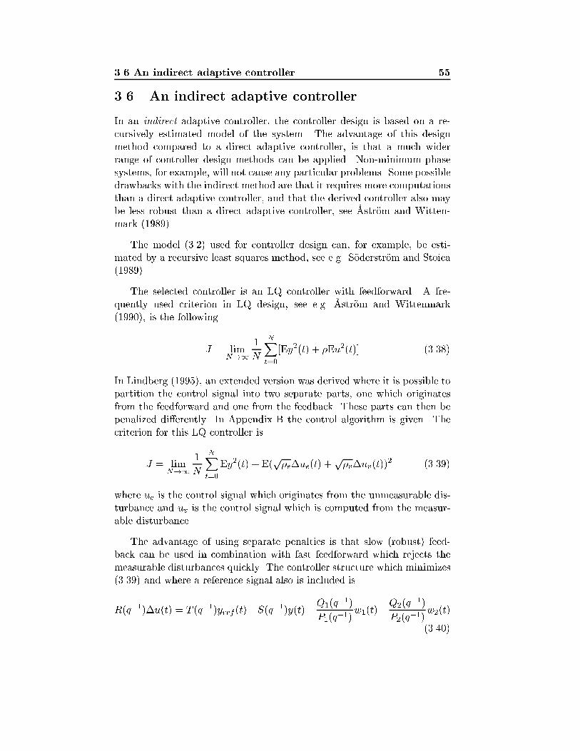
3.6 An indirect adaptive controller 55
3.6 An indirect adaptive controller
In an indirect adaptive controller, the controller design is based on a re-cursively estimated model of the system. The advantage of this designmethod compared to a direct adaptive controller, is that a much widerrange of controller design methods can be applied. Non-minimum phasesystems, for example, will not cause any particular problems. Some possibledrawbacks with the indirect method are that it requires more computationsthan a direct adaptive controller, and that the derived controller also maybe less robust than a direct adaptive controller, see �Astr�om and Witten-mark (1989).
The model (3.2) used for controller design can, for example, be esti-mated by a recursive least squares method, see e.g. S�oderstr�om and Stoica(1989).
The selected controller is an LQ controller with feedforward. A fre-quently used criterion in LQ design, see e.g. �Astr�om and Wittenmark(1990), is the following
J = limN!1
1
N
NXt=0
[Ey2(t) + �Eu2(t)] (3.38)
In Lindberg (1995), an extended version was derived where it is possible topartition the control signal into two separate parts, one which originatesfrom the feedforward and one from the feedback. These parts can then bepenalized di�erently. In Appendix B the control algorithm is given. Thecriterion for this LQ controller is
J = limN!1
1
N
NXt=0
Ey2(t) + E(p�e�ue(t) +
p�v�uv(t))
2 (3.39)
where ue is the control signal which originates from the unmeasurable dis-turbance and uv is the control signal which is computed from the measur-able disturbance.
The advantage of using separate penalties is that slow (robust) feed-back can be used in combination with fast feedforward which rejects themeasurable disturbances quickly. The controller structure which minimizes(3.39) and where a reference signal also is included is
R(q�1)�u(t) = T (q�1)yref (t)�S(q�1)y(t)�Q1(q�1)
P1(q�1)w1(t)�Q2(q
�1)
P2(q�1)w2(t)
(3.40)
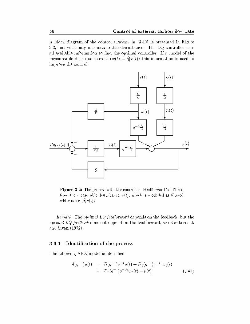
56 Control of external carbon ow rate
A block diagram of the control strategy in (3.40) is presented in Figure3.2, but with only one measurable disturbance. The LQ controller usesall available information to �nd the optimal controller. If a model of themeasureable disturbance exist (w(t) = G
Hv(t)) this information is used to
improve the control.
m m
QP
1R� q�k B
A
?-
6
- - - -
�S
q�d DA
CA
1�
GH
����HHHj
?
�
?
? ?
�
�+
n(t)
e(t)v(t)
y(t)u(t)
w(t)
Tyref (t)
Figure 3.2: The process with the controller. Feedforward is utilized
from the measurable disturbance w(t), which is modelled as �ltered
white noise (GHv(t)).
Remark: The optimal LQ feedforward depends on the feedback, but theoptimal LQ feedback does not depend on the feedforward, see Kwakernaakand Sivan (1972).
3.6.1 Identi�cation of the process
The following ARX model is identi�ed
A(q�1)y(t) = B(q�1)q�ku(t) +D1(q�1)q�d1w1(t)
+ D2(q�1)q�d2w2(t) + n(t) (3.41)
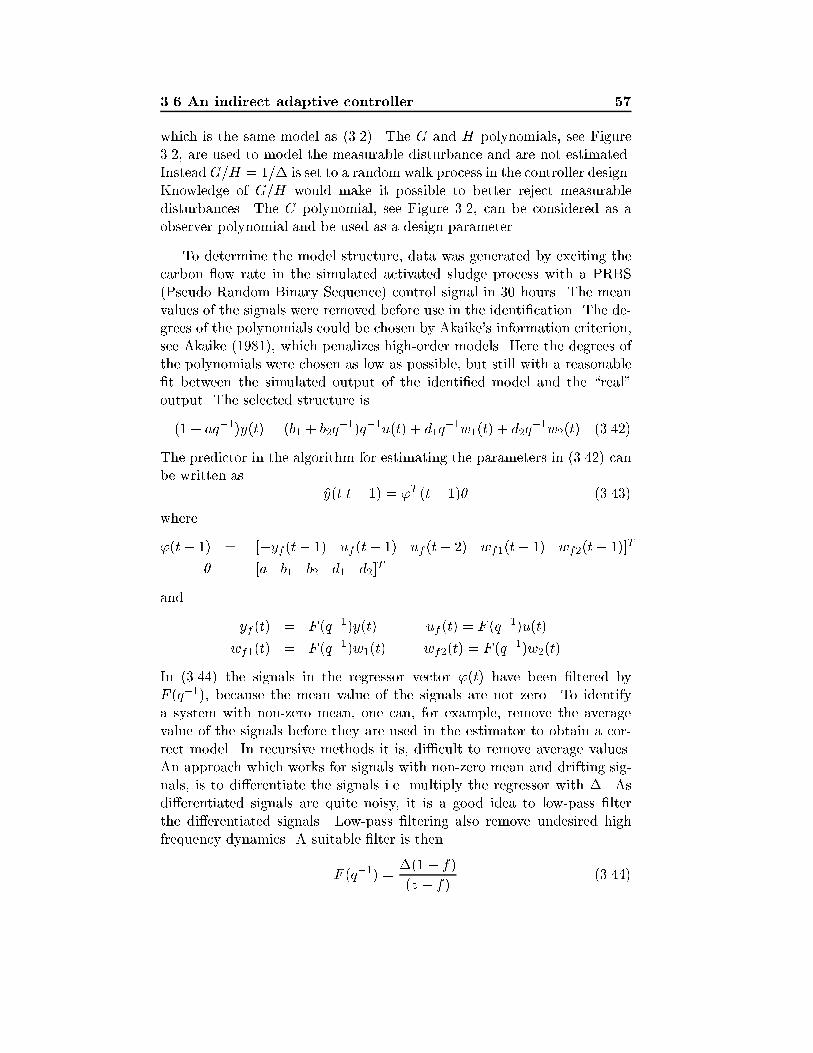
3.6 An indirect adaptive controller 57
which is the same model as (3.2). The G and H polynomials, see Figure3.2, are used to model the measurable disturbance and are not estimated.InsteadG=H = 1=� is set to a random walk process in the controller design.Knowledge of G=H would make it possible to better reject measurabledisturbances. The C polynomial, see Figure 3.2, can be considered as aobserver polynomial and be used as a design parameter.
To determine the model structure, data was generated by exciting thecarbon ow rate in the simulated activated sludge process with a PRBS(Pseudo Random Binary Sequence) control signal in 30 hours. The meanvalues of the signals were removed before use in the identi�cation. The de-grees of the polynomials could be chosen by Akaike's information criterion,see Akaike (1981), which penalizes high-order models. Here the degrees ofthe polynomials were chosen as low as possible, but still with a reasonable�t between the simulated output of the identi�ed model and the \real"output. The selected structure is
(1 + aq�1)y(t) = (b1 + b2q�1)q�1u(t) + d1q
�1w1(t) + d2q�1w2(t) (3.42)
The predictor in the algorithm for estimating the parameters in (3.42) canbe written as
y(tjt� 1) = 'T (t� 1)� (3.43)
where
'(t� 1) = [�yf (t� 1) uf (t� 1) uf (t� 2) wf1(t� 1) wf2(t� 1)]T
� = [a b1 b2 d1 d2]T
and
yf (t) = F (q�1)y(t) uf (t) = F (q�1)u(t)
wf1(t) = F (q�1)w1(t) wf2(t) = F (q�1)w2(t)
In (3.44) the signals in the regressor vector '(t) have been �ltered byF (q�1), because the mean value of the signals are not zero. To identifya system with non-zero mean, one can, for example, remove the averagevalue of the signals before they are used in the estimator to obtain a cor-rect model. In recursive methods it is, di�cult to remove average values.An approach which works for signals with non-zero mean and drifting sig-nals, is to di�erentiate the signals i.e. multiply the regressor with �. Asdi�erentiated signals are quite noisy, it is a good idea to low-pass �lterthe di�erentiated signals. Low-pass �ltering also remove undesired highfrequency dynamics. A suitable �lter is then
F (q�1) =�(1� f)
(z � f)(3.44)
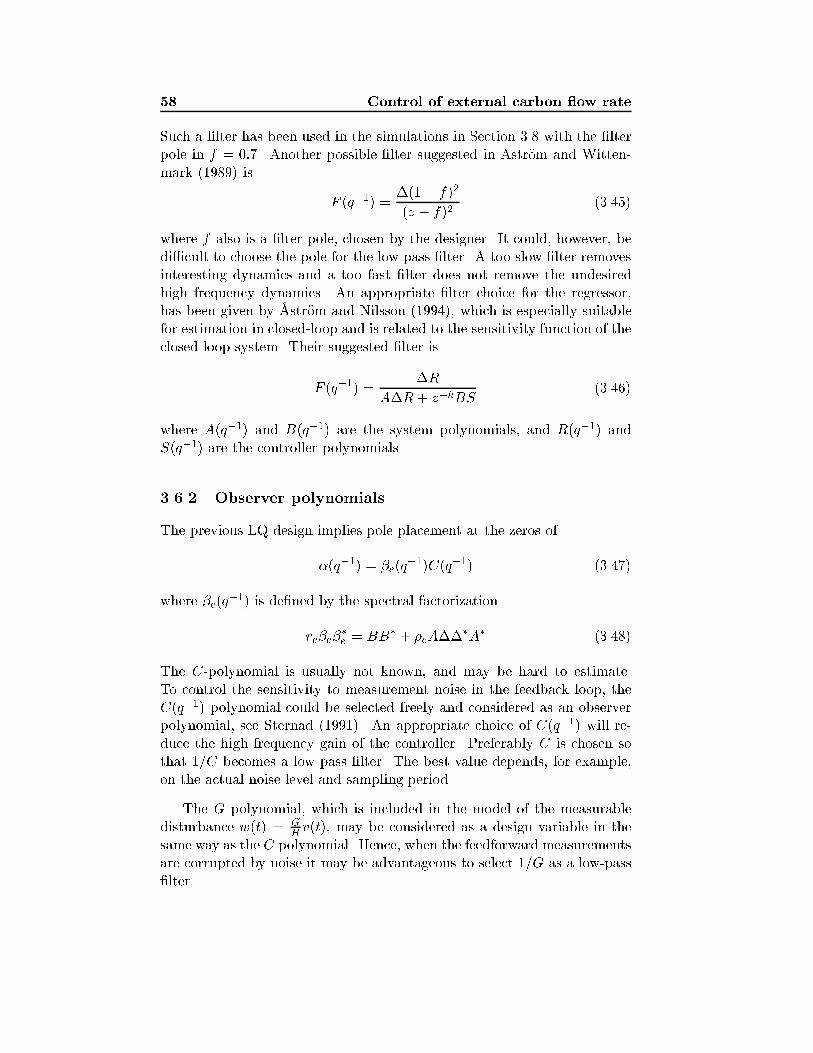
58 Control of external carbon ow rate
Such a �lter has been used in the simulations in Section 3.8 with the �lterpole in f = 0:7. Another possible �lter suggested in �Astr�om and Witten-mark (1989) is
F (q�1) =�(1� f)2
(z � f)2(3.45)
where f also is a �lter pole, chosen by the designer. It could, however, bedi�cult to choose the pole for the low pass �lter. A too slow �lter removesinteresting dynamics and a too fast �lter does not remove the undesiredhigh frequency dynamics. An appropriate �lter choice for the regressor,has been given by �Astr�om and Nilsson (1994), which is especially suitablefor estimation in closed-loop and is related to the sensitivity function of theclosed-loop system. Their suggested �lter is
F (q�1) =�R
A�R+ z�kBS(3.46)
where A(q�1) and B(q�1) are the system polynomials, and R(q�1) andS(q�1) are the controller polynomials.
3.6.2 Observer polynomials
The previous LQ design implies pole placement at the zeros of
�(q�1) = �e(q�1)C(q�1) (3.47)
where �e(q�1) is de�ned by the spectral factorization
re�e��e = BB� + �eA��
�A� (3.48)
The C-polynomial is usually not known, and may be hard to estimate.To control the sensitivity to measurement noise in the feedback loop, theC(q�1) polynomial could be selected freely and considered as an observerpolynomial, see Sternad (1991). An appropriate choice of C(q�1) will re-duce the high frequency gain of the controller. Preferably C is chosen sothat 1=C becomes a low pass �lter. The best value depends, for example,on the actual noise level and sampling period.
The G polynomial, which is included in the model of the measurabledisturbance w(t) = G
Hv(t), may be considered as a design variable in the
same way as the C polynomial. Hence, when the feedforward measurementsare corrupted by noise it may be advantageous to select 1=G as a low-pass�lter.
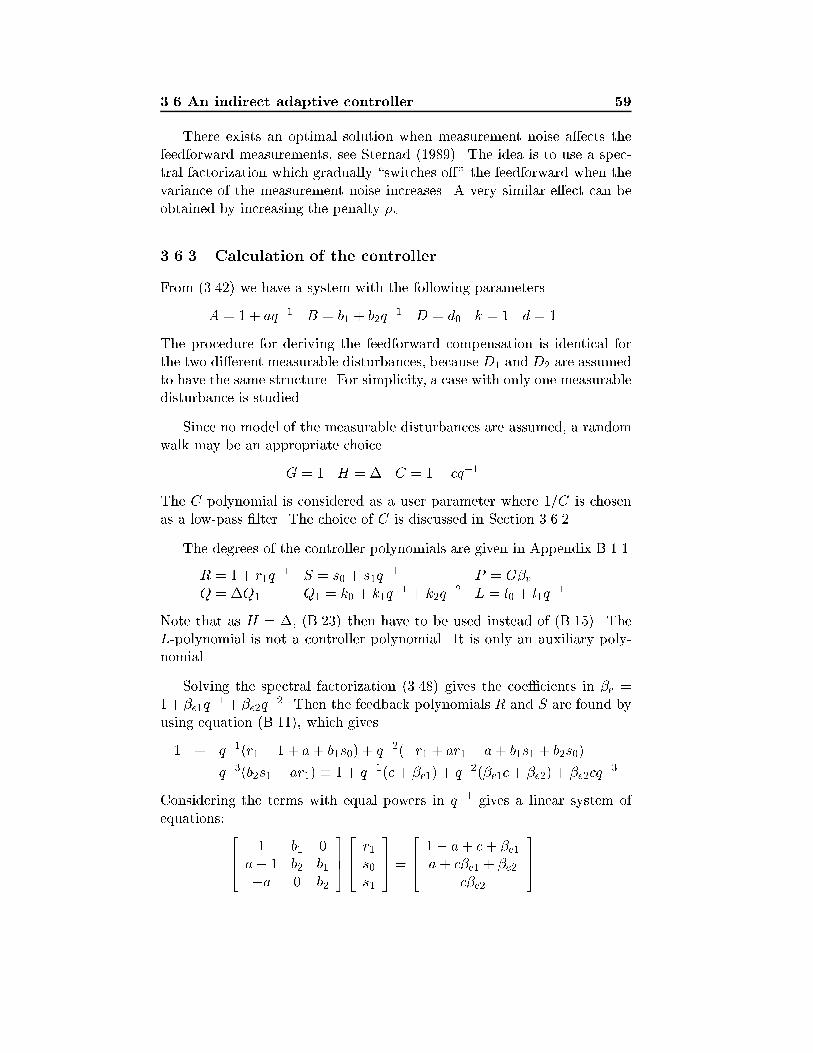
3.6 An indirect adaptive controller 59
There exists an optimal solution when measurement noise a�ects thefeedforward measurements, see Sternad (1989). The idea is to use a spec-tral factorization which gradually \switches o�" the feedforward when thevariance of the measurement noise increases. A very similar e�ect can beobtained by increasing the penalty �v.
3.6.3 Calculation of the controller
From (3.42) we have a system with the following parameters
A = 1 + aq�1 B = b1 + b2q�1 D = d0 k = 1 d = 1
The procedure for deriving the feedforward compensation is identical forthe two di�erent measurable disturbances, because D1 and D2 are assumedto have the same structure. For simplicity, a case with only one measurabledisturbance is studied.
Since no model of the measurable disturbances are assumed, a randomwalk may be an appropriate choice.
G = 1 H = � C = 1 + cq�1
The C polynomial is considered as a user parameter where 1=C is chosenas a low-pass �lter. The choice of C is discussed in Section 3.6.2.
The degrees of the controller polynomials are given in Appendix B.1.1
R = 1 + r1q�1 S = s0 + s1q
�1 P = G�vQ = �Q1 Q1 = k0 + k1q
�1 + k2q�2 L = l0 + l1q
�1
Note that as H = �, (B.23) then have to be used instead of (B.15). TheL-polynomial is not a controller polynomial. It is only an auxiliary poly-nomial.
Solving the spectral factorization (3.48) gives the coe�cients in �e =1+�e1q
�1+�e2q�2. Then the feedback polynomials R and S are found by
using equation (B.11), which gives
1 + q�1(r1 � 1 + a+ b1s0) + q�2(�r1 + ar1 � a+ b1s1 + b2s0)
+ q�3(b2s1 � ar1) � 1 + q�1(c+ �e1) + q�2(�e1c+ �e2) + �e2cq�3
Considering the terms with equal powers in q�1 gives a linear system ofequations: 264 1 b1 0
a� 1 b2 b1�a 0 b2
375264 r1s0s1
375 =264 1� a+ c+ �e1a+ c�e1 + �e2
c�e2
375
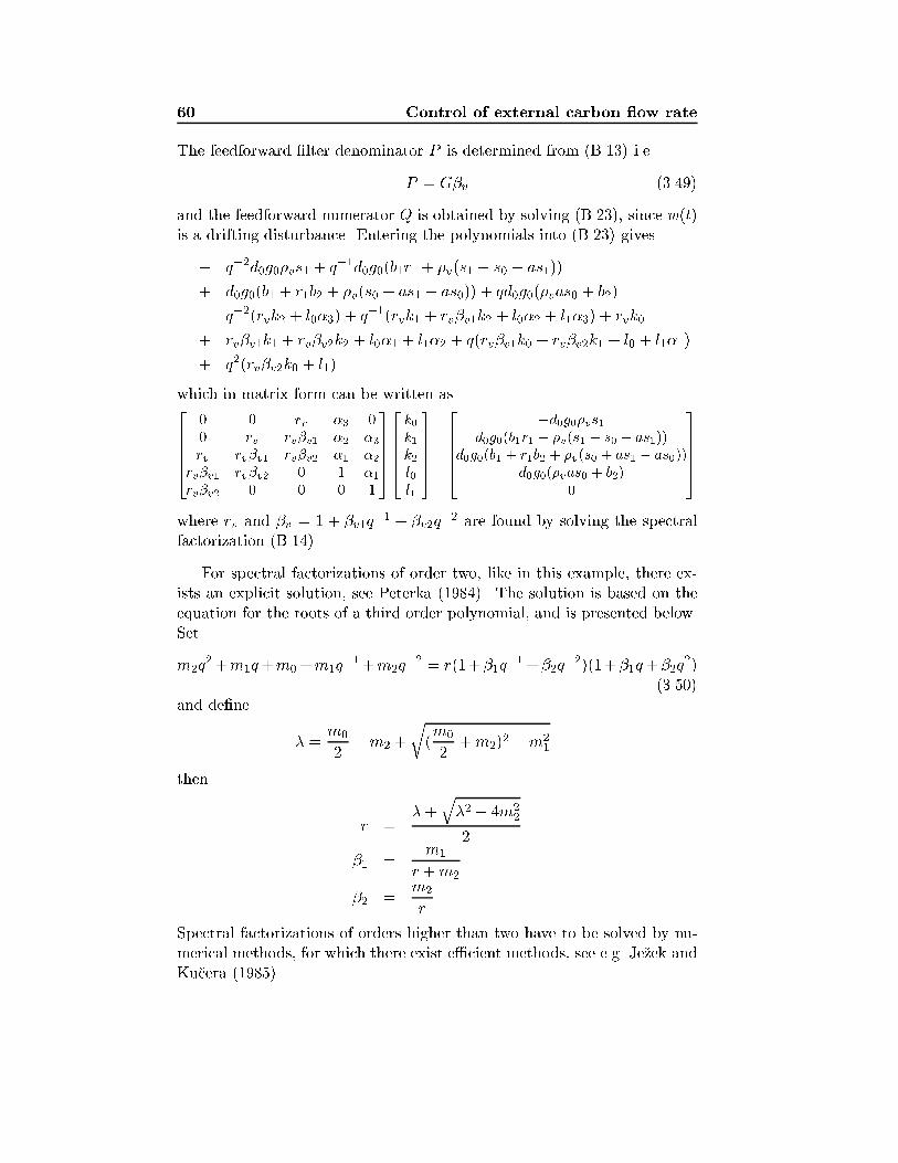
60 Control of external carbon ow rate
The feedforward �lter denominator P is determined from (B.13) i.e.
P = G�v (3.49)
and the feedforward numerator Q is obtained by solving (B.23), since w(t)is a drifting disturbance. Entering the polynomials into (B.23) gives
� q�2d0g0�vs1 + q�1d0g0(b1r1 + �v(s1 � s0 � as1))
+ d0g0(b1 + r1b2 + �v(s0 + as1 � as0)) + qd0g0(�vas0 + b2)
= q�2(rvk2 + l0�3) + q�1(rvk1 + rv�v1k2 + l0�2 + l1�3) + rvk0
+ rv�v1k1 + rv�v2k2 + l0�1 + l1�2 + q(rv�v1k0 + rv�v2k1 + l0 + l1�1)
+ q2(rv�v2k0 + l1)
which in matrix form can be written as2666640 0 rv �3 00 rv rv�v1 �2 �3rv rv�v1 rv�v2 �1 �2
rv�v1 rv�v2 0 1 �1rv�v2 0 0 0 1
377775266664k0k1k2l0l1
377775=266664
�d0g0�vs1d0g0(b1r1 + �v(s1 � s0 � as1))
d0g0(b1 + r1b2 + �v(s0 + as1 � as0))d0g0(�vas0 + b2)
0
377775where rv and �v = 1 + �v1q
�1 + �v2q�2 are found by solving the spectral
factorization (B.14).
For spectral factorizations of order two, like in this example, there ex-ists an explicit solution, see Peterka (1984). The solution is based on theequation for the roots of a third order polynomial, and is presented below.Set
m2q2+m1q+m0+m1q
�1+m2q�2 = r(1+�1q
�1+�2q�2)(1+�1q+�2q
2)(3.50)
and de�ne
� =m0
2�m2 +
r(m0
2+m2)2 �m2
1
then
r =�+
q�2 � 4m2
2
2
�1 =m1
r +m2
�2 =m2
r
Spectral factorizations of orders higher than two have to be solved by nu-merical methods, for which there exist e�cient methods, see e.g. Je�zek andKu�cera (1985).
3.7 Practical aspects for the adaptive controllers 61
Remark: When deriving the control signal, one may instead of multi-plying Q1 with � and then obtaining (Q1�)w(t) = Qw(t), di�erentiatew(t) and then let Q1 operate on �w(t).
3.7 Practical aspects for the adaptive controllers
Some important problems in adaptive control and their (possible) solutionswill considered in this section.
3.7.1 Potter's square root algorithm
When updating the parameters in a recursive algorithm, the covariance ma-trix P (t) is used. To avoid numerical problems with accumulating roundingerrors and which leads to P (t) becoming inde�nite, Potter's square root al-gorithm can be used, see e.g. Ljung and S�oderstr�om (1983).
De�ne the matrix S(t) through
P (t) = S(t)ST (t) (3.51)
and update S(t) instead of P (t) as
f(t) = ST (t� 1)'(t) (3.52)
�(t) = �+ fT (t)f(t) (3.53)
�(t) =1
�(t) +p�(t)�
(3.54)
L(t) = S(t� 1)f(t) (3.55)
S(t) =S(t� 1)� �(t)L(t)fT (t)p
�(3.56)
The parameter estimates are then updated as
�(t) = �(t� 1) + L(t)"(t)
�(t)(3.57)
Note that there will be less computations in (3.57) if "(t) is divided by �(t)before it is multiplied by L(t).
If Potter's algorithm is not used, the diagonal elements of P (t) couldbe checked instead. The matrix P (t) should always be positive de�nite,which means that all diagonal elements of P (t) always must be larger thanzero. If they are not, P (t) can be set to an identity matrix times a smallconstant. Note that positive diagonal elements does not guarantee thatP (t) is positive de�nite, but this test is at least better than no checking atall.
62 Control of external carbon ow rate
3.7.2 Choice of initial covariance matrix and initial regres-sor
The initial covariance matrix P (0) should re ect the uncertainty of theparameter vector. Usually the uncertainty is large and P (0) could be chosenas P (0) = �2I, where � is a large value which in is related to the varianceof the elements in the ' vector, and the parameter vector is set to �(0) = 0.Note that the regressor '(t) has to be �lled with \real signal values" beforethe estimation algorithm can be started. Otherwise the parameters takehuge steps in wrong directions, and it may then be hard or impossible forthe parameters to recover to reasonable values.
It is also a good idea to disconnect the controller and replace the controlsignal with a PRBS signal, for example, and then only run the estimatorduring the �rst 30-50 samples. This gives the system a high excitation andthe parameters can better converge. Note that this is only possible if theopen loop system is stable.
3.7.3 The forgetting factor �
The forgetting factor � should re ect the parameter variations in the realprocess. To determine � one could use the relation for the memory length,which is approximately equal to 2=(1 � �). A value of � between 0.95 and0.998 is often suitable. When there is little noise and few parameters areestimated a smaller � can be selected. In the simulations � = 0:95 wasused.
3.7.4 Estimator windup
A common problem when using a forgetting factor � < 1 is estimatorwindup, which makes the covariance matrix P (t) grow exponentially duringperiods with low excitation. An example of estimator windup is shown inFigure 3.3. It is the indirect adaptive controller with feedforward, appliedto control the nitrate concentration. Note that the scale in Figure 3.3 forthe trace of the covariance matrix is logarithmic. As seen, the trace ofP (t) grows exponentially, during low excitation, and when the system isexcited again the estimated parameters take a too large step. The systemcontrolled by this controller (not shown) has very bad performance.
There exist di�erent methods to avoid estimator windup. One feasi-ble strategy to reduce the problem, which is used here, is a combinationof the algorithm suggested in Ahl�en and Sternad (1988) and �Astr�om and
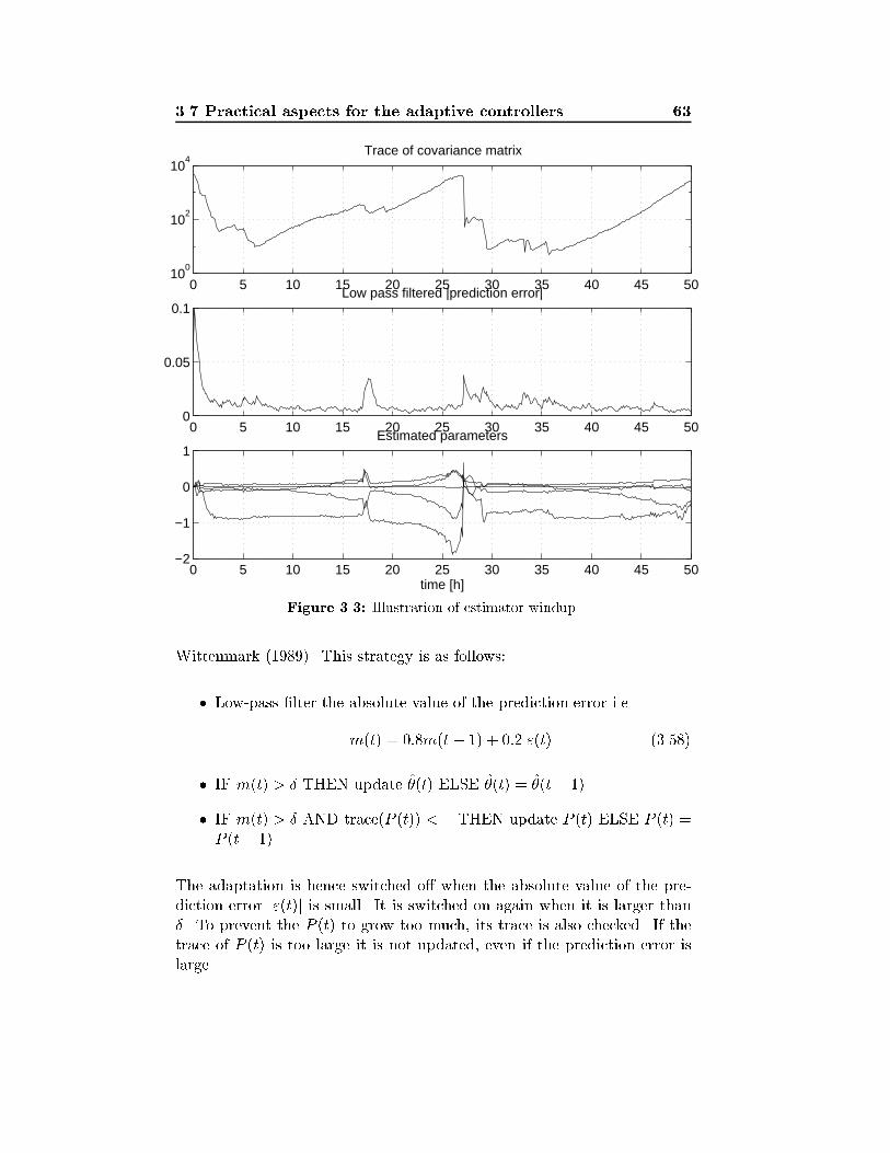
3.7 Practical aspects for the adaptive controllers 63
0 5 10 15 20 25 30 35 40 45 5010
0
102
104
Trace of covariance matrix
0 5 10 15 20 25 30 35 40 45 500
0.05
0.1Low pass filtered |prediction error|
0 5 10 15 20 25 30 35 40 45 50−2
−1
0
1Estimated parameters
time [h]
Figure 3.3: Illustration of estimator windup.
Wittenmark (1989). This strategy is as follows:
� Low-pass �lter the absolute value of the prediction error i.e.
m(t) = 0:8m(t � 1) + 0:2j"(t)j (3.58)
� IF m(t) > � THEN update �(t) ELSE �(t) = �(t� 1)
� IF m(t) > � AND trace(P (t)) < � THEN update P (t) ELSE P (t) =P (t� 1)
The adaptation is hence switched o� when the absolute value of the pre-diction error j"(t)j is small. It is switched on again when it is larger than�. To prevent the P (t) to grow too much, its trace is also checked. If thetrace of P (t) is too large it is not updated, even if the prediction error islarge.
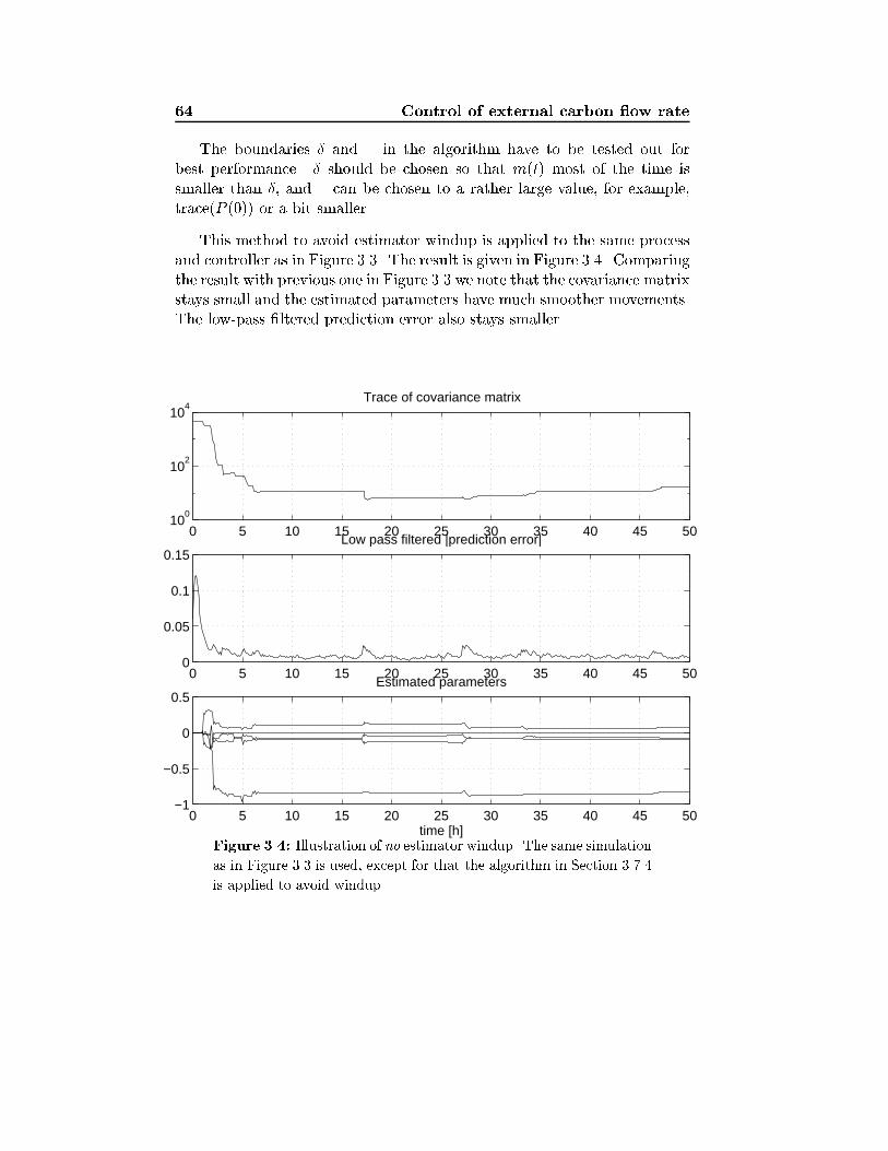
64 Control of external carbon ow rate
The boundaries � and � in the algorithm have to be tested out forbest performance. � should be chosen so that m(t) most of the time issmaller than �, and � can be chosen to a rather large value, for example,trace(P (0)) or a bit smaller.
This method to avoid estimator windup is applied to the same processand controller as in Figure 3.3. The result is given in Figure 3.4. Comparingthe result with previous one in Figure 3.3 we note that the covariance matrixstays small and the estimated parameters have much smoother movements.The low-pass �ltered prediction error also stays smaller.
0 5 10 15 20 25 30 35 40 45 5010
0
102
104
Trace of covariance matrix
0 5 10 15 20 25 30 35 40 45 500
0.05
0.1
0.15Low pass filtered |prediction error|
0 5 10 15 20 25 30 35 40 45 50−1
−0.5
0
0.5Estimated parameters
time [h]Figure 3.4: Illustration of no estimator windup. The same simulation
as in Figure 3.3 is used, except for that the algorithm in Section 3.7.4
is applied to avoid windup.
3.7 Practical aspects for the adaptive controllers 65
3.7.5 Scaling the regressors
If the estimated parameters di�ers much in size, e.g. more than a factor 10,then the signal in the regressor can be scaled. This improves the numericalproperties and the estimates, see also �Astr�om and Wittenmark (1989).
3.7.6 Including the reference signal
The direct adaptive controller is extended with a reference signal yref(t) inthe following way
(R(q�1) +�
r0C(q�1))�u(t) = T (q�1)yref(t)� S(q�1)y(t)�Q(q�1)�w(t)
(3.59)and the indirect adaptive controller in this way
R(q�1)�u(t) = T (q�1)yref (t)� S(q�1)y(t)� Q(q�1)
P (q�1)w(t) (3.60)
The T (q�1) polynomial �lters the reference signal and may be chosen to
T (q�1) = mC(q�1) (3.61)
where m is a constant which is selected to obtain the static gain equal toone. This is obtained by choosing
m =�e(1)
B(1)=S(1)
C(1)(3.62)
where �e is de�ned in the spectral factorization (3.48). This choice of m isfound by deriving the closed loop system from yref (t) to y(t), which is
y(t) =q�kBT
AR�+ q�kBSyref(t) (3.63)
and by using AR�+ q�kBS = �eC, together with �(1) = 0.
For the direct controller, the identity (3.24) can be used to determine theclosed loop denominator AR�+ q�kBS, which then becomes BC. Hence,if C(q�1) = 1 then T = S(1) = C(1) = 1. It may, however, happen thatS(1) 6= 1. It is then better to use T = S(1), because this makes the staticgain more safer equal to one.
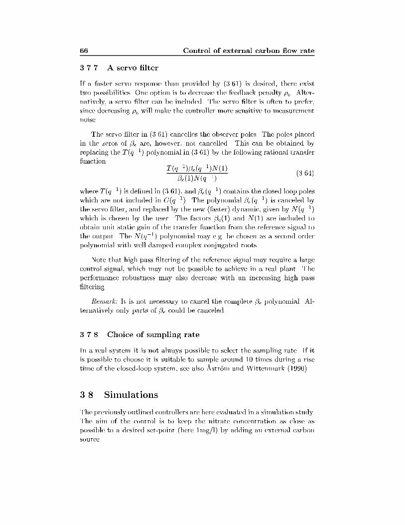
66 Control of external carbon ow rate
3.7.7 A servo �lter
If a faster servo response than provided by (3.61) is desired, there existtwo possibilities. One option is to decrease the feedback penalty �e. Alter-natively, a servo �lter can be included. The servo �lter is often to prefer,since decreasing �e will make the controller more sensitive to measurementnoise.
The servo �lter in (3.61) cancelles the observer poles. The poles placedin the zeros of �e are, however, not cancelled. This can be obtained byreplacing the T (q�1) polynomial in (3.61) by the following rational transferfunction
T (q�1)�e(q�1)N(1)
�e(1)N(q�1)(3.64)
where T (q�1) is de�ned in (3.61), and �e(q�1) contains the closed loop poles
which are not included in C(q�1). The polynomial �e(q�1) is canceled by
the servo �lter, and replaced by the new (faster) dynamic, given by N(q�1)which is chosen by the user. The factors �e(1) and N(1) are included toobtain unit static gain of the transfer function from the reference signal tothe output. The N(q�1) polynomial may e.g. be chosen as a second orderpolynomial with well damped complex conjugated roots.
Note that high pass �ltering of the reference signal may require a largecontrol signal, which may not be possible to achieve in a real plant. Theperformance robustness may also decrease with an increasing high pass�ltering.
Remark: It is not necessary to cancel the complete �e polynomial. Al-ternatively only parts of �e could be canceled.
3.7.8 Choice of sampling rate
In a real system it is not always possible to select the sampling rate. If itis possible to choose it is suitable to sample around 10 times during a risetime of the closed-loop system, see also �Astr�om and Wittenmark (1990).
3.8 Simulations
The previously outlined controllers are here evaluated in a simulation study.The aim of the control is to keep the nitrate concentration as close aspossible to a desired set-point (here 1mg/l) by adding an external carbonsource.
3.8 Simulations 67
3.8.1 Simulation setup for the activated sludge process
In all simulations, the true process is simulated by the model presented inChapter 2.3 with the following exceptions:
� Measurement noise: Zero mean white noise with standard deviation0.1 is added to the nitrate measurements.
� Flows and concentrations: The ows and concentrations presented inFigure 3.5 are used, all other ows and concentrations are the defaultones in Section 2.3.
0 5 10 15 20 25 30 35 400
0.2
0.4
0.6
0.8
time [h]
m^3
/h
Influent flow (−) and internal recirculation (−−)
0 5 10 15 20 25 30 35 4010
20
30
40
50
60
70
time [h]
mg/
l
Influent substrate (−) and influent ammonium (−−)
Figure 3.5: Variations in in uent ow, internal recirculation, in uent
soluble substrate and in uent ammonium during the simulation.
3.8.2 PI control
A PI-controller with feedforward is used here to control the nitrate level inthe anoxic zone. The PI controller is tuned based on pole placement, usingan estimated linear process model
(1 + aq�1)y(t) = bu(t� 1) (3.65)
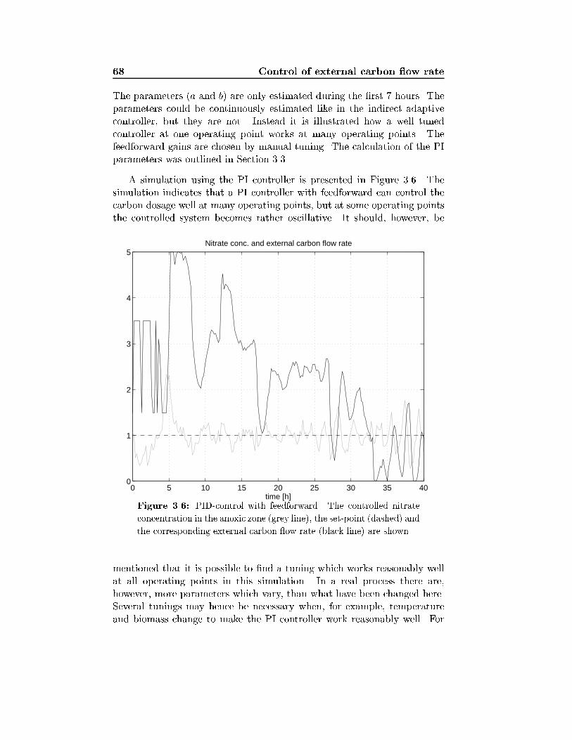
68 Control of external carbon ow rate
The parameters (a and b) are only estimated during the �rst 7 hours. Theparameters could be continuously estimated like in the indirect adaptivecontroller, but they are not. Instead it is illustrated how a well tunedcontroller at one operating point works at many operating points. Thefeedforward gains are chosen by manual tuning. The calculation of the PIparameters was outlined in Section 3.3.
A simulation using the PI controller is presented in Figure 3.6. Thesimulation indicates that a PI controller with feedforward can control thecarbon dosage well at many operating points, but at some operating pointsthe controlled system becomes rather oscillative. It should, however, be
0 5 10 15 20 25 30 35 400
1
2
3
4
5
time [h]
Nitrate conc. and external carbon flow rate
Figure 3.6: PID-control with feedforward. The controlled nitrate
concentration in the anoxic zone (grey line), the set-point (dashed) and
the corresponding external carbon ow rate (black line) are shown.
mentioned that it is possible to �nd a tuning which works reasonably wellat all operating points in this simulation. In a real process there are,however, more parameters which vary, than what have been changed here.Several tunings may hence be necessary when, for example, temperatureand biomass change to make the PI controller work reasonably well. For
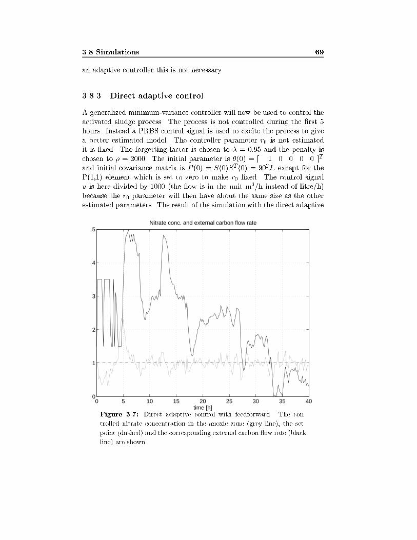
3.8 Simulations 69
an adaptive controller this is not necessary.
3.8.3 Direct adaptive control
A generalized minimum-variance controller will now be used to control theactivated sludge process. The process is not controlled during the �rst 5hours. Instead a PRBS control signal is used to excite the process to givea better estimated model. The controller parameter r0 is not estimatedit is �xed. The forgetting factor is chosen to � = 0:95 and the penalty ischosen to � = 2000. The initial parameter is �(0) = [ �1 0 0 0 0 ]T
and initial covariance matrix is P (0) = S(0)ST (0) = 902I, except for theP(1,1) element which is set to zero to make r0 �xed. The control signalu is here divided by 1000 (the ow is in the unit m3/h instead of litre/h)because the r0 parameter will then have about the same size as the otherestimated parameters. The result of the simulation with the direct adaptive
0 5 10 15 20 25 30 35 400
1
2
3
4
5
time [h]
Nitrate conc. and external carbon flow rate
Figure 3.7: Direct adaptive control with feedforward. The con-
trolled nitrate concentration in the anoxic zone (grey line), the set-
point (dashed) and the corresponding external carbon ow rate (black
line) are shown.
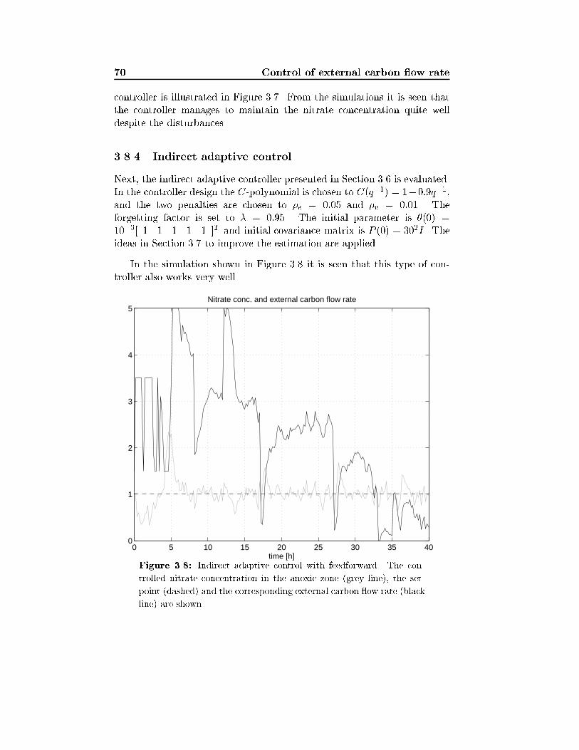
70 Control of external carbon ow rate
controller is illustrated in Figure 3.7. From the simulations it is seen thatthe controller manages to maintain the nitrate concentration quite welldespite the disturbances.
3.8.4 Indirect adaptive control
Next, the indirect adaptive controller presented in Section 3.6 is evaluated.In the controller design the C-polynomial is chosen to C(q�1) = 1�0:9q�1,and the two penalties are chosen to �e = 0:05 and �v = 0:01. Theforgetting factor is set to � = 0:95. The initial parameter is �(0) =10�3[ 1 1 1 1 1 ]T and initial covariance matrix is P (0) = 302I. Theideas in Section 3.7 to improve the estimation are applied.
In the simulation shown in Figure 3.8 it is seen that this type of con-troller also works very well.
0 5 10 15 20 25 30 35 400
1
2
3
4
5
time [h]
Nitrate conc. and external carbon flow rate
Figure 3.8: Indirect adaptive control with feedforward. The con-
trolled nitrate concentration in the anoxic zone (grey line), the set-
point (dashed) and the corresponding external carbon ow rate (black
line) are shown.
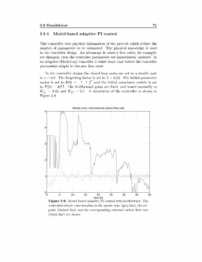
3.8 Simulations 71
3.8.5 Model-based adaptive PI control
This controller uses physical information of the process which reduce thenumber of parameters to be estimated. The physical knowledge is usedin the controller design. An advantage is when a ow rates, for example,are changed, then the controller parameters are immediately updated. Inan adaptive (black-box) controller it takes some time before the controllerparameters adapts to the new ow rates.
In the controller design the closed loop poles are set to a double polein z = 0:8. The forgetting factor is set to � = 0:95. The initial parametervector is set to �(0) = [ 1 1 ]T and the initial covariance matrix is setto P (0) = 302I. The feedforward gains are �xed, and tuned manually toKf1 = 0:05 and Kf2 = 0:7. A simulation of the controller is shown inFigure 3.9.
0 5 10 15 20 25 30 35 400
1
2
3
4
5
time [h]
Nitrate conc. and external carbon flow rate
Figure 3.9: Model-based adaptive PI control with feedforward. The
controlled nitrate concentration in the anoxic zone (grey line), the set-
point (dashed line) and the corresponding external carbon ow rate
(black line) are shown.
72 Control of external carbon ow rate
Remark 1: Using the same model, an LQ controller with feedforwardcould be also be designed, but this has not been considered here.
Remark 2: One idea to maintain the dynamic for the nitrate concentra-tion model could be to vary the sampling rate when the ow rates changes.For a system with the following dynamic
y(t+ 1) = y(t) +Qh
V(u(t)� y(t))
the discrete-time transfer function is constant, if the variations in Q arecompensated with variations in the sampling interval h, i.e. Qh is keptconstant. A problem with this approach on the carbon dosage dynamics,is that a change in the sampling rate a�ects many parameters. It hence isnot obvious if this approach could introduce a simpli�cation.
3.8.6 Extended model-based adaptive PI control
This controller uses some extensions compared to the model-based adaptivePI control, and it was described in Section 3.4.1.
In the controller design the closed loop poles are set to a double polein z = 0:8. The forgetting factor is set to � = 0:95. The initial parameteris set to �(0) = 0:1 and the initial covariance matrix is set to P (0) = 302.The feedforward gain is �xed and tuned manually to Kf1 = 0:07
The performance is similar to the model-based adaptive PI controller,but since this controller take the nonlinearity of the SS concentration intoaccount, the variations in the control signal becomes larger during distur-bances in the ow rate, as seen in Figure 3.10. The higest peaks are notshown in this �gure, but in Figure 3.11 it is shown that the maximumamplitude of the control signal is around 10 l/h.
This or the model-based adaptive PI controller has probably the bestperformance.
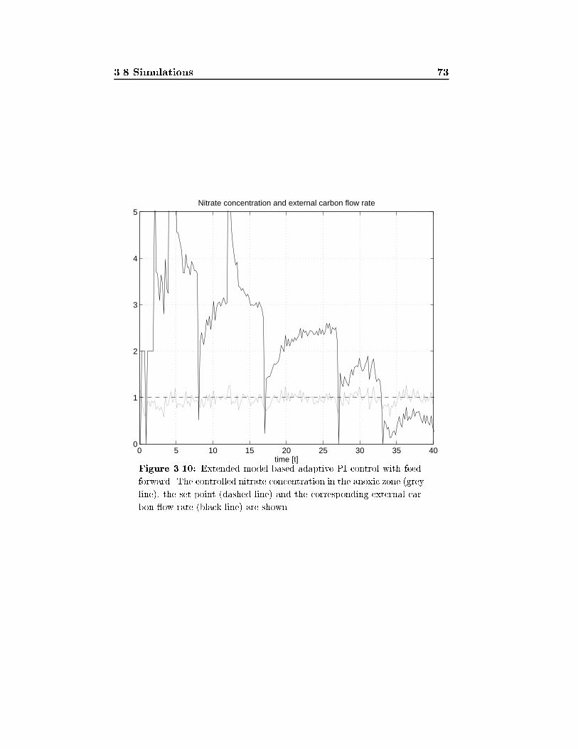
3.8 Simulations 73
0 5 10 15 20 25 30 35 400
1
2
3
4
5
time [t]
Nitrate concentration and external carbon flow rate
Figure 3.10: Extended model-based adaptive PI control with feed-
forward. The controlled nitrate concentration in the anoxic zone (grey
line), the set-point (dashed line) and the corresponding external car-
bon ow rate (black line) are shown.

74 Control of external carbon ow rate
3.8.7 Illustration of feedforward
Two comparisons with and without feedforward are simulated here. Inthe �rst comparison the model-based PI controller with and without feed-forward is studied. In the second comparison an indirect adaptive LQcontroller is studied.
The controllers use the same initialization as in Section 3.8.6 and Section3.8.4, but measurement noise is set to zero to make the di�erence betweenthe two strategies easier to see. Another di�erence is that the model-basedPI controller is tuned slower, the closed loop poles in 0.85 instead of 0.8.
In Figure 3.11 a simulation with the model-based PI controller is shown.
0 5 10 15 20 25 30 35 400
1
2
time [t]
mg/
l
Nitrate concentration
0 5 10 15 20 25 30 35 400
2
4
6
8
10
time [t]
l/h
External carbon flow rate
Figure 3.11: Illustration of a controller with and without feedforward
for the model-based PI controller. The solid lines correspond to the
controller with feedforward, and the dashed lines to the controller
without feedforward. The set-point line is dotted.
The controller rejects, as expected, the disturbances faster with feedfor-ward. The ow rate disturbances seem, however, very hard to reject. De-spite large variations (notches) in control signal, these disturbances are not
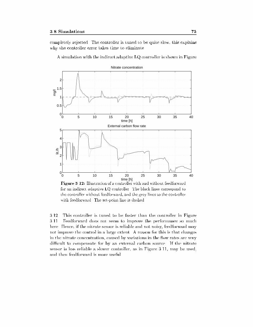
3.8 Simulations 75
completely rejected. The controller is tuned to be quite slow, this explainswhy the controller error takes time to eliminate.
A simulation with the indirect adaptive LQ controller is shown in Figure
0 5 10 15 20 25 30 35 400
0.5
1
1.5
2
time [h]
mg/
l
Nitrate concentration
0 5 10 15 20 25 30 35 400
1
2
3
4
5
time [h]
lit./h
External carbon flow rate
Figure 3.12: Illustration of a controller with and without feedforward
for an indirect adaptive LQ controller. The black lines correspond to
the controller without feedforward, and the grey lines to the controller
with feedforward. The set-point line is dashed.
3.12. This controller is tuned to be faster than the controller in Figure3.11. Feedforward does not seem to improve the performance so muchhere. Hence, if the nitrate sensor is reliable and not noisy, feedforward maynot improve the control in a large extent. A reason for this is that changesin the nitrate concentration, caused by variations in the ow rates are verydi�cult to compensate for by an external carbon source. If the nitratesensor is less reliable a slower controller, as in Figure 3.11, may be used,and then feedforward is more useful.
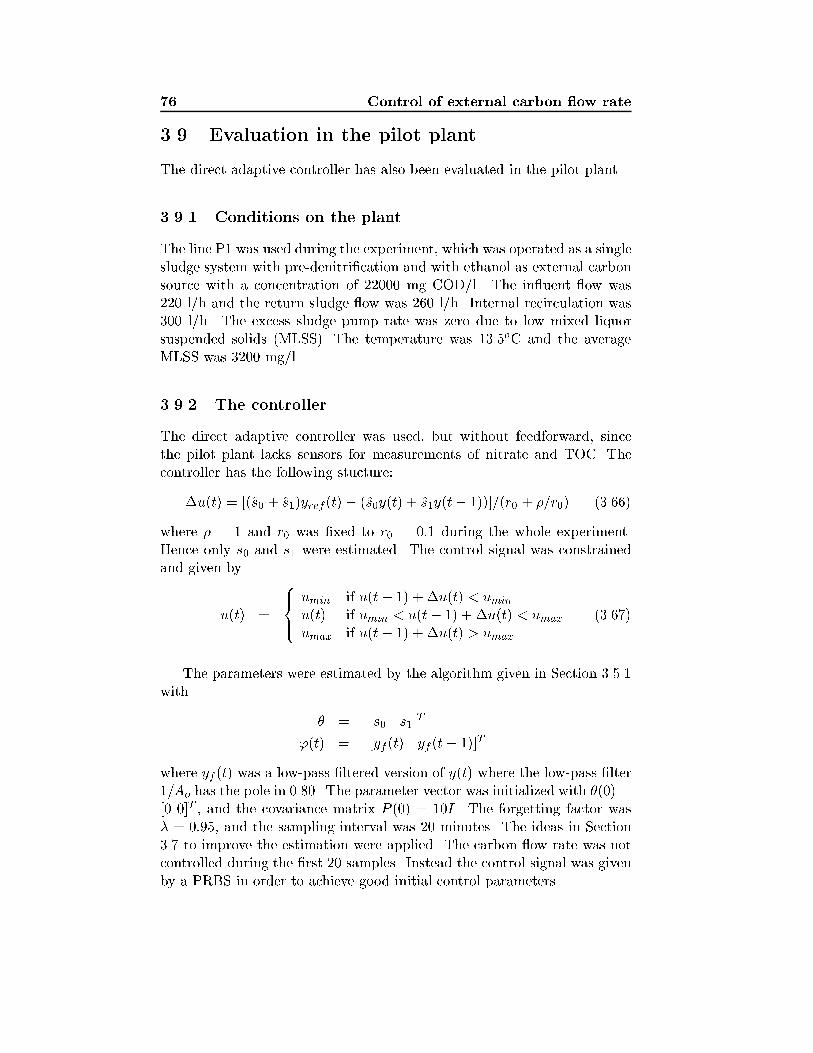
76 Control of external carbon ow rate
3.9 Evaluation in the pilot plant
The direct adaptive controller has also been evaluated in the pilot plant.
3.9.1 Conditions on the plant
The line P1 was used during the experiment, which was operated as a singlesludge system with pre-denitri�cation and with ethanol as external carbonsource with a concentration of 22000 mg COD/l. The in uent ow was220 l/h and the return sludge ow was 260 l/h. Internal recirculation was300 l/h. The excess sludge pump rate was zero due to low mixed liquorsuspended solids (MLSS). The temperature was 13.5oC and the averageMLSS was 3200 mg/l.
3.9.2 The controller
The direct adaptive controller was used, but without feedforward, sincethe pilot plant lacks sensors for measurements of nitrate and TOC. Thecontroller has the following stucture:
�u(t) = [(s0 + s1)yref(t)� (s0y(t) + s1y(t� 1))]=(r0 + �=r0) (3.66)
where � = 1 and r0 was �xed to r0 = 0:1 during the whole experiment.Hence only s0 and s1 were estimated. The control signal was constrainedand given by
u(t) =
8><>:umin if u(t� 1) + �u(t) < uminu(t) if umin < u(t� 1) + �u(t) < umaxumax if u(t� 1) + �u(t) > umax
(3.67)
The parameters were estimated by the algorithm given in Section 3.5.1with
� = [s0 s1]T
'(t) = [yf (t) yf (t� 1)]T
where yf (t) was a low-pass �ltered version of y(t) where the low-pass �lter1=Ao has the pole in 0.80. The parameter vector was initialized with �(0) =[0 0]T , and the covariance matrix P (0) = 10I. The forgetting factor was� = 0:95, and the sampling interval was 20 minutes. The ideas in Section3.7 to improve the estimation were applied. The carbon ow rate was notcontrolled during the �rst 20 samples. Instead the control signal was givenby a PRBS in order to achieve good initial control parameters.
3.9 Evaluation in the pilot plant 77
3.9.3 Results
The experiment with the adaptive controller is presented in Figure 3.13.The di�erent events which occured during the test period (18 { 26 Jan1996) is described in Table 3.1.
0 1 2 3 4 5 6 7 8 90
2
4
6
8
time [days]
[mg/
l]
Nitrate conc. in anoxic zone and effluent
0 1 2 3 4 5 6 7 8 90
0.5
1
1.5
2
2.5
time [days]
[l/h]
Carbon dosage
Figure 3.13: Upper plot: Nitrate concentration in the anoxic zone
(solid line) and in e�uent water (dotted line). Lower plot: The carbon
ow rate. The carbon source has the conc. 22000 mg COD/l.
Due to a malfunction, starting around day 5, in the real plant, the CODconcentration in the in uent water to the pilot-scale plant increased fromapproximately 200 mg COD/l to 600 mg COD/l. This may explain thedecreased carbon ow rate at the end of the experiment. This problemmay also have masked the e�ect of the changes made in the in ow rate, seeTable 3.1.
The controller performed quite well despite the rather noisy nitratesensor, and it also rejected disturbances well. The latter can be seen bythe behavior when the sensor is calibrated (the sensor output then goesabruptly down). It is also interesting to study the variations of carbon ow
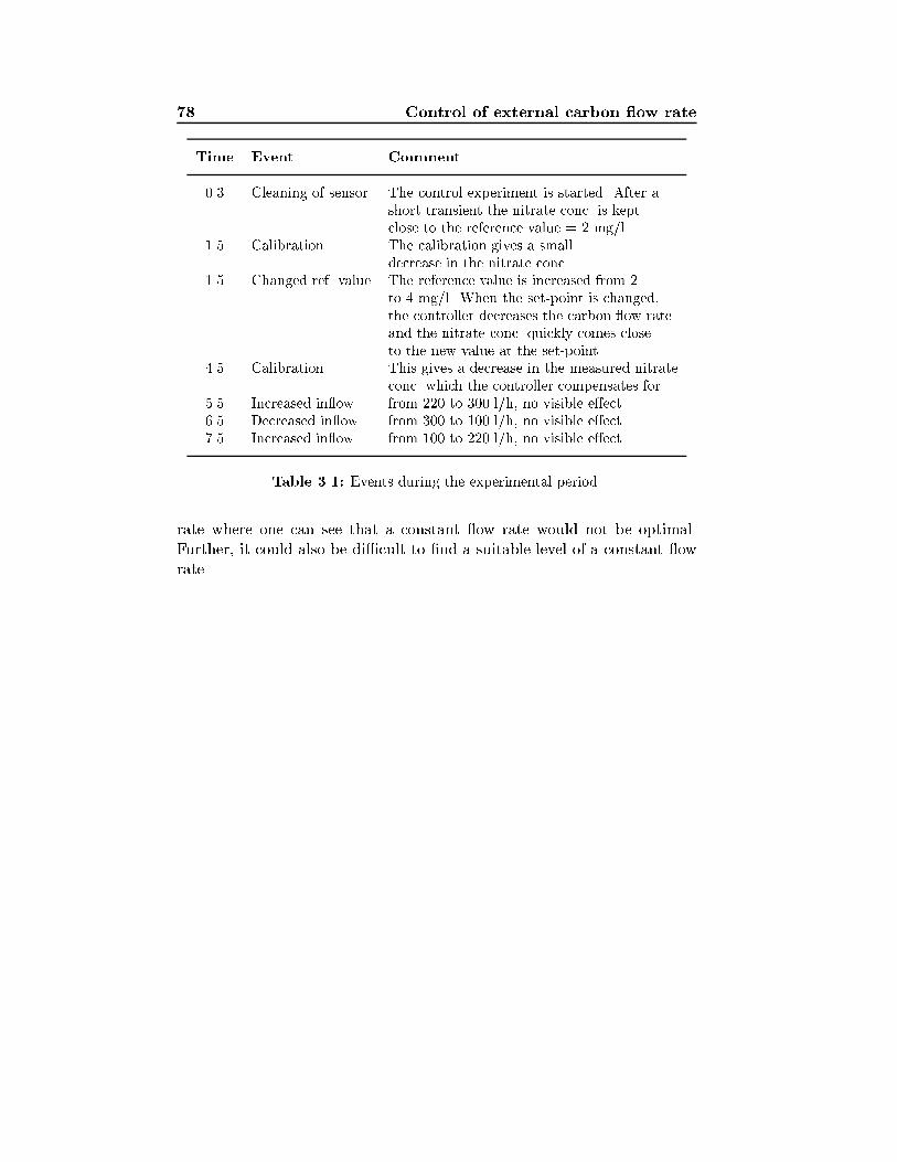
78 Control of external carbon ow rate
Time Event Comment
0.3 Cleaning of sensor The control experiment is started. After ashort transient the nitrate conc. is keptclose to the reference value = 2 mg/l.
1.5 Calibration The calibration gives a smalldecrease in the nitrate conc.
1.5 Changed ref. value The reference value is increased from 2to 4 mg/l. When the set-point is changed,the controller decreases the carbon ow rateand the nitrate conc. quickly comes closeto the new value at the set-point.
4.5 Calibration This gives a decrease in the measured nitrateconc. which the controller compensates for.
5.5 Increased in ow from 220 to 300 l/h, no visible e�ect6.5 Decreased in ow from 300 to 100 l/h, no visible e�ect7.5 Increased in ow from 100 to 220 l/h, no visible e�ect
Table 3.1: Events during the experimental period.
rate where one can see that a constant ow rate would not be optimal.Further, it could also be di�cult to �nd a suitable level of a constant owrate.
3.10 Conclusions 79
3.10 Conclusions
In this chapter four di�erent types of controllers for the external carbon ow rate have been evaluated by means of simulation studies. One of thecontrollers was also tested in a practical experiment.
The evaluated controllers were a PID-controller, a generalized minimum-variance (direct adaptive) controller, an indirect adaptive controller, anda model-based PI controller. All controllers used feedforward from therecirculated nitrate mass ow and in uent TOC mass ow. The controlstrategy was based on keeping the nitrate concentration in the anoxic zoneat a constant and low level.
It can be concluded that all four controllers have similar performancefor control of the nitrate concentration. Any of them may hence be a usefultool for a more pertinent control of the activated sludge process.
Some individual comments about the controllers could, however, begiven:
� The PID-controller gave reasonably good control. It was easy toimplement but it may be di�cult to tune. It may also give poorcontrol when the process is time-varying and may then even becomeunstable.
� The direct adaptive controller gave reasonably good performance andadapts well to changes in the process.
� The indirect adaptive controller also gave reasonably good perfor-mance and adapted well to changes in the process. The estimatedprocess model can be be used for a wide range of controller designs.This means that unstable and non-minimum phase systems are of noparticular problem. A drawback is that the suggested LQ controlleris more complex and requires more computations than the other con-trollers.
� The model-based adaptive PI controller has high control performance.It used much physical information about the process and few param-eters needed to be estimated. By using physical knowledge of theprocess in the controller design, the controller could, for example,immediately update the controller parameters when there is a changein a ow rate.
The adaptive controllers requires a safety net to work properly. The safety

80 Control of external carbon ow rate
net was described and simulations have shown that the adaptive controllerswork well.
A practical experiment with the direct adaptive controller has also beenperformed. It showed that the direct adaptive controller managed well tocontrol the nitrate concentration in the anoxic zone.
A possible extension could be to control the reference value of the nitrateconcentration in the anoxic zone so that the e�uent nitrate could be keptat a constant and low level.
Chapter 4
Estimation of the dissolved
oxygen concentration
dynamics
In this chapter methods for estimating two essential parameters which char-acterize the dissolved oxygen concentration (DO) dynamics in an activatedsludge process are presented. The two variables are the respiration rateR(t), and the oxygen transfer function KLa. The name oxygen transferfunction is chosen to stress that it depends on several variables. Othercommon names in the literature are e.g. oxygen transfer rate and masstransfer coe�cient. Knowledge of these two variables are of interest inboth process diagnosis, Olsson and Andrews (1978), and process controlincluding dissolved oxygen control, see, e.g., Spanjers (1993), Klapwijk et
al. (1993), Spanjers et al. (1996) and Lindberg and Carlsson (1996d).
The respiration rate is the key variable that characterizes the DO pro-cess and the associated removal and degradation of biodegradable matter.It is the only true indicator of biologically degradable load, Holmberg et al.(1989). If toxic matter enters the plant, for example, this can be detectedas a decrease in the respiration rate, since the microorganisms slow downtheir activity or some of them die. A rapid decrease in the respiration ratemay hence be used as a warning that toxic matter has entered the plant anda by-pass action may be taken to save the microorganisms. The respirationrate can also be used for improved DO control, see Chapter 5. For morecontrol applications using the respiration rate, see Spanjers et al. (1996).
The oxygen transfer function KLa (actually it is KLa(u)(yset�y)) de-
82 Estimation of the DO dynamics
scribes the rate with which oxygen is transferred to the activated sludgeby the aeration system. The KLa function can be expected to be nonlin-ear and it depends on several factors. Here, only its main time-varyingdependence is considered, namely the air ow rate.
To �nd the respiration rate and theKLa function one could e.g. do batchtests, use a respirometer (the respirometer do not measure KLa) or applyan estimation algorithm (software sensor). The latter method is used here.The estimation algorithm is based on measurements of the dissolved oxygenconcentration and the air ow rate which are used as inputs to a Kalman�lter. Several estimation approaches have been suggested e.g. by Holmberg(1981), Ko et al. (1982), Holmberg and Olsson (1985), Holmberg et al.
(1989), Bocken et al. (1989), Cook and Jowitt (1985), Carlsson and Wigren(1993), Carlsson et al. (1994a) and Lukasse et al. (1996). Many of theseapproaches have used simpli�ed assumptions. For example, the respirationrate is assumed to be time invariant, or the oxygen transfer function is alinear function or a linear trend of the air ow rate. In Holmberg (1990)it was argued that a linear trend model of KLa leads to identi�abilityproblems. Here a method is suggested which may avoid these problems.The simpli�ed assumptions are not used, and also, the DO sensor dynamicsis considered.
In the suggested estimation scheme, two models of the nonlinear KLafunction are suggested, an exponential function and a cubic spline function.For other possible parameterizations of KLa, see Lindberg and Carlsson(1993). Di�erent models of the time-varying respiration rate are studied.In particular, a �ltered random walk model is considered, including twospecial cases: a random walk model and an integrated random walk model.These cases are obtained by speci�c choices of the �lter pole in the modelfor describing the time variation. TheKLa function and the respiration rateare tracked by a Kalman �lter by using the measurements of air ow rateand DO, see also Holmberg and Olsson (1985) and Ljung and S�oderstr�om(1983).
When estimating the respiration rate and oxygen transfer function frommeasurements of DO and air ow rates, it is necessary that a high excitationin the air ow rate, both in frequency and amplitude, is used. A high excita-tion of the air ow rate, implies rapid changes in DO. If the DO sensor is notfast, the estimates will be biased. A �ltering procedure developed by Ahl�enand Sternad (1989) is applied to reduce the in uence of the DO sensor dy-namics. The �ltered DO measurements can then be used for estimating therespiration rate and the oxygen transfer function. The suggested method issuccessfully illustrated both in simulations and on real data from the pilot
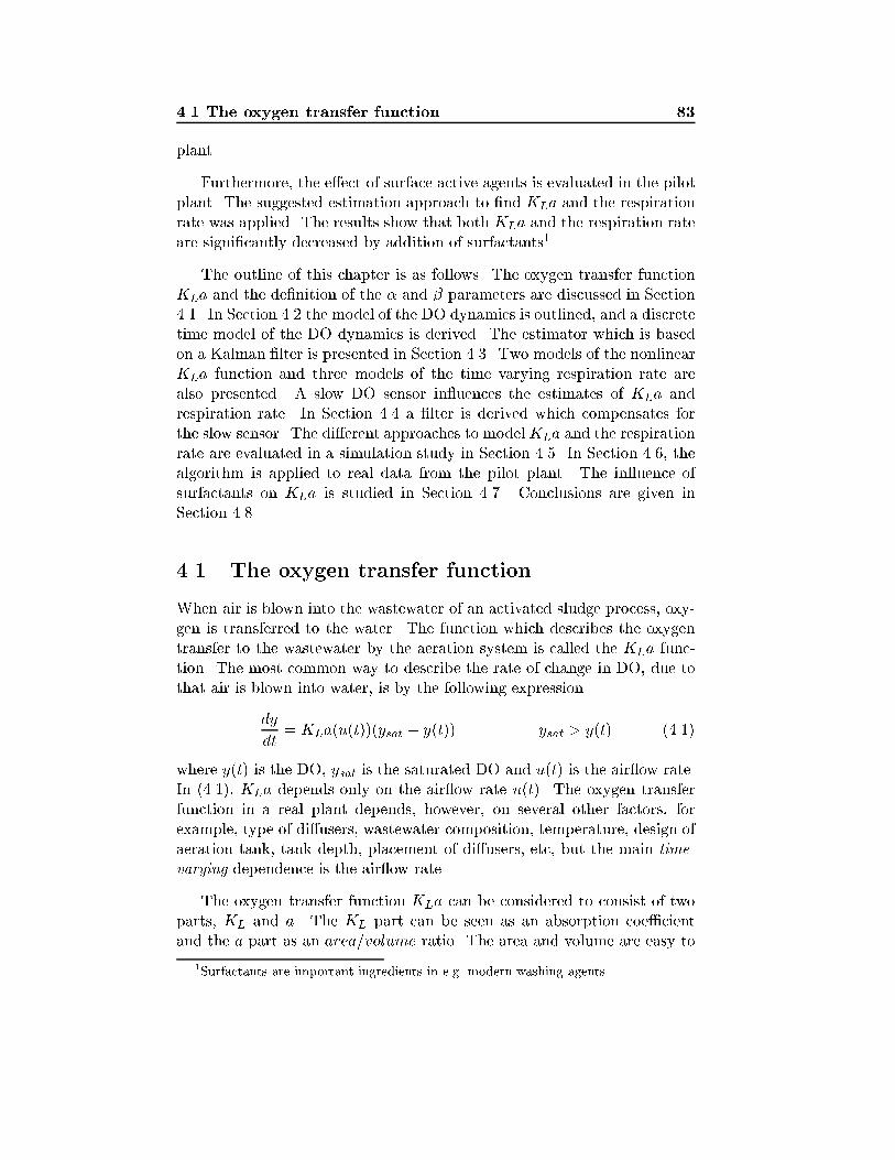
4.1 The oxygen transfer function 83
plant.
Furthermore, the e�ect of surface active agents is evaluated in the pilotplant. The suggested estimation approach to �nd KLa and the respirationrate was applied. The results show that both KLa and the respiration rateare signi�cantly decreased by addition of surfactants1.
The outline of this chapter is as follows. The oxygen transfer functionKLa and the de�nition of the � and � parameters are discussed in Section4.1. In Section 4.2 the model of the DO dynamics is outlined, and a discretetime model of the DO dynamics is derived. The estimator which is basedon a Kalman �lter is presented in Section 4.3. Two models of the nonlinearKLa function and three models of the time varying respiration rate arealso presented. A slow DO sensor in uences the estimates of KLa andrespiration rate. In Section 4.4 a �lter is derived which compensates forthe slow sensor. The di�erent approaches to modelKLa and the respirationrate are evaluated in a simulation study in Section 4.5. In Section 4.6, thealgorithm is applied to real data from the pilot plant. The in uence ofsurfactants on KLa is studied in Section 4.7. Conclusions are given inSection 4.8.
4.1 The oxygen transfer function
When air is blown into the wastewater of an activated sludge process, oxy-gen is transferred to the water. The function which describes the oxygentransfer to the wastewater by the aeration system is called the KLa func-tion. The most common way to describe the rate of change in DO, due tothat air is blown into water, is by the following expression
dy
dt= KLa(u(t))(ysat � y(t)) ysat > y(t) (4.1)
where y(t) is the DO, ysat is the saturated DO and u(t) is the air ow rate.In (4.1), KLa depends only on the air ow rate u(t). The oxygen transferfunction in a real plant depends, however, on several other factors, forexample, type of di�users, wastewater composition, temperature, design ofaeration tank, tank depth, placement of di�users, etc, but the main time-
varying dependence is the air ow rate.
The oxygen transfer function KLa can be considered to consist of twoparts, KL and a. The KL part can be seen as an absorption coe�cientand the a part as an area=volume ratio. The area and volume are easy to
1Surfactants are important ingredients in e.g. modern washing agents.
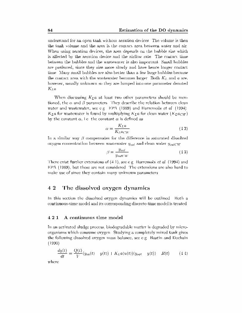
84 Estimation of the DO dynamics
understand for an open tank without aeration devices. The volume is thenthe tank volume and the area is the contact area between water and air.When using aeration devices, the area depends on the bubble size whichis a�ected by the aeration device and the air ow rate. The contact timebetween the bubbles and the wastewater is also important. Small bubblesare preferred, since they rise more slowly and have hence longer contacttime. Many small bubbles are also better than a few large bubbles becausethe contact area with the wastewater becomes larger. Both KL and a are,however, usually unknown so they are lumped into one parameter denotedKLa.
When discussing KLa at least two other parameters should be men-tioned, the � and � parameters. They describe the relation between cleanwater and wastewater, see e.g. EPA (1989) and Harremo�es et al. (1994).KLa for wastewater is found by multiplyingKLa for clean water (KLaCW )by the constant �, i.e. the constant � is de�ned as
� =KLa
KLaCW(4.2)
In a similar way � compensates for the di�erence in saturated dissolvedoxygen concentration between wastewater ysat and clean water ysatCW
� =ysat
ysatCW(4.3)
There exist further extensions of (4.1), see e.g. Harremo�es et al. (1994) andEPA (1989), but these are not considered. The extensions are also hard tomake use of since they contain many unknown parameters.
4.2 The dissolved oxygen dynamics
In this section the dissolved oxygen dynamics will be outlined. Both acontinuous-time model and its corresponding discrete-time model is treated.
4.2.1 A continuous time model
In an activated sludge process, biodegradable matter is degraded by micro-organisms which consume oxygen. Studying a completely mixed tank givesthe following dissolved oxygen mass balance, see e.g. Bastin and Dochain(1990)
dy(t)
dt=Q(t)
V(yin(t)� y(t)) +KLa(u(t))(ysat � y(t))�R(t) (4.4)
where
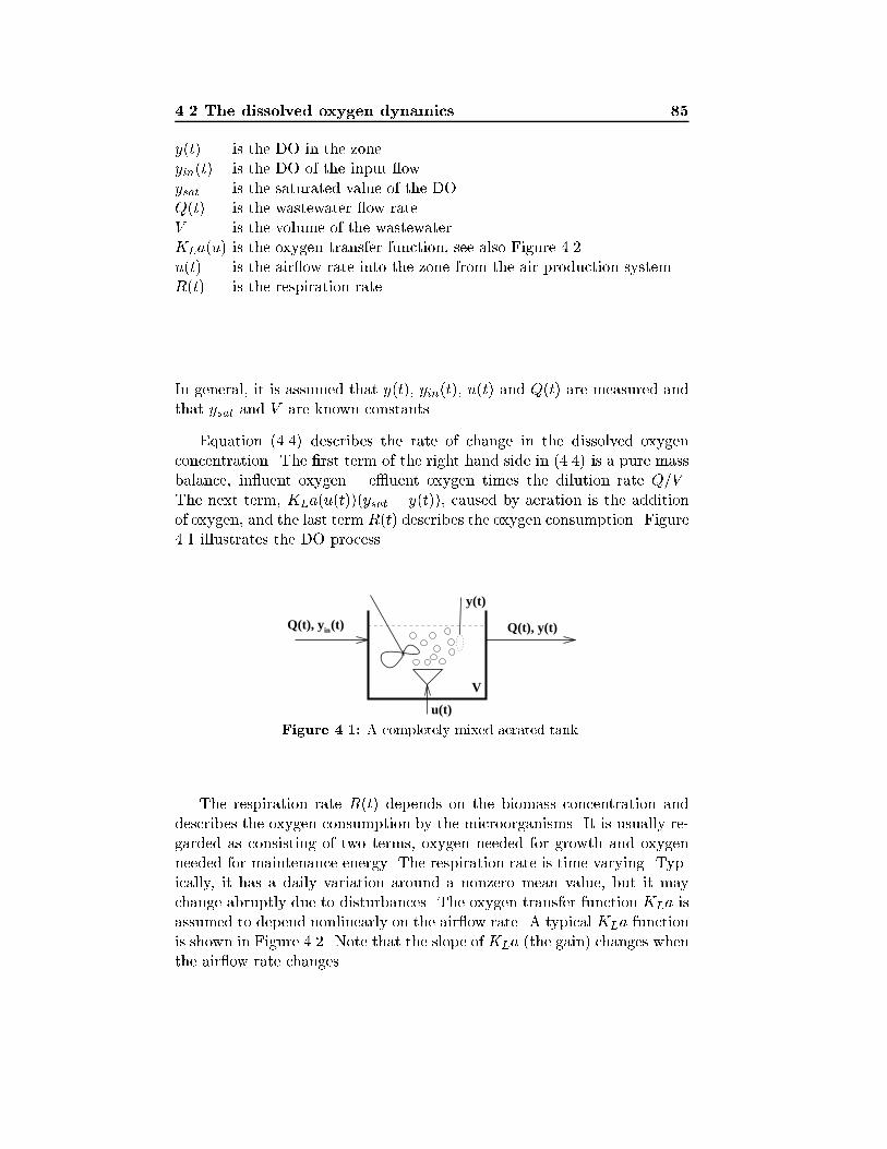
4.2 The dissolved oxygen dynamics 85
y(t) is the DO in the zoneyin(t) is the DO of the input owysat is the saturated value of the DOQ(t) is the wastewater ow rateV is the volume of the wastewaterKLa(u) is the oxygen transfer function, see also Figure 4.2u(t) is the air ow rate into the zone from the air production systemR(t) is the respiration rate
In general, it is assumed that y(t), yin(t), u(t) and Q(t) are measured andthat ysat and V are known constants.
Equation (4.4) describes the rate of change in the dissolved oxygenconcentration. The �rst term of the right hand side in (4.4) is a pure massbalance, in uent oxygen { e�uent oxygen times the dilution rate Q=V .The next term, KLa(u(t))(ysat � y(t)), caused by aeration is the additionof oxygen, and the last term R(t) describes the oxygen consumption. Figure4.1 illustrates the DO process.
Q(t), y(t)
V
Q(t), yin(t)
u(t)
y(t)
Figure 4.1: A completely mixed aerated tank.
The respiration rate R(t) depends on the biomass concentration anddescribes the oxygen consumption by the microorganisms. It is usually re-garded as consisting of two terms, oxygen needed for growth and oxygenneeded for maintenance energy. The respiration rate is time-varying. Typ-ically, it has a daily variation around a nonzero mean value, but it maychange abruptly due to disturbances. The oxygen transfer function KLa isassumed to depend nonlinearly on the air ow rate. A typical KLa functionis shown in Figure 4.2. Note that the slope of KLa (the gain) changes whenthe air ow rate changes.
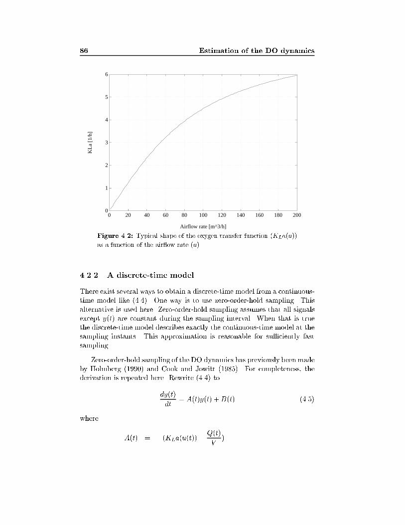
86 Estimation of the DO dynamics
0
1
2
3
4
5
6
0 20 40 60 80 100 120 140 160 180 200
Airflow rate [m^3/h]
KL
a [1
/h]
Figure 4.2: Typical shape of the oxygen transfer function (KLa(u))
as a function of the air ow rate (u).
4.2.2 A discrete-time model
There exist several ways to obtain a discrete-time model from a continuous-time model like (4.4). One way is to use zero-order-hold sampling. Thisalternative is used here. Zero-order-hold sampling assumes that all signalsexcept y(t) are constant during the sampling interval. When that is truethe discrete-time model describes exactly the continuous-time model at thesampling instants. This approximation is reasonable for su�ciently fastsampling.
Zero-order-hold sampling of the DO dynamics has previously been madeby Holmberg (1990) and Cook and Jowitt (1985). For completeness, thederivation is repeated here. Rewrite (4.4) to
dy(t)
dt= A(t)y(t) +B(t) (4.5)
where
A(t) = �(KLa(u(t)) +Q(t)
V)

4.3 The estimator 87
B(t) = �R(t) + Q(t)
Vyin(t) +KLa(u(t))ysat
Assuming that A(t) and B(t) are constant within each sampling period,model (4.5) is sampled by using theory in, for example, �Astr�om and Wit-tenmark (1990) which gives
y(kh+ h)) = eA(kh)hy(kh) +B(kh)
A(kh)(eA(kh)h � 1) (4.6)
where h is the sampling interval and k is the discrete time. Now set
h� =1
A(kh)(eA(kh)h � 1) (4.7)
and the sampled model becomes
y(kh+ h)) � y(kh)
h�= A(kh)y(kh) +B(kh) (4.8)
In the following we will for notational simplicity replace kh with t. Thisgives together with A and B inserted in (4.8)
y(t+1) = y(t)+h�[Q(t)
V(yin(t)�y(t))+KLa(u(t))(ysat�y(t))�R(t)]+w(t)
(4.9)In (4.9), a term w(t) has been added to describe measurement noise andmodel mis�t.
4.3 The estimator
What makes it nontrivial to identify the dissolved oxygen dynamics is that
� The respiration rate R(t) is time-varying.
� The oxygen transfer function KLa is nonlinear.
� The absolute levels of the respiration rate and KLa are hard touniquely determine.
� The DO sensor may have a signi�cant dynamics.
A possible remedy to the above problems is
� Use a Kalman �lter approach to track the time-varying respirationrate.
88 Estimation of the DO dynamics
� Use the three following assumptions regarding the KLa function:
A1 The oxygen transfer function KLa can be su�ciently well de-scribed by a static nonlinearity of the air ow rate u(t).
A2 The parameters in the KLa model change slowly in comparisonwith the respiration rate.
A3 The oxygen transfer function is zero when the air ow rate is zero,i.e. KLa(0) = 0, see Carlsson and Wigren (1993) and Carlssonet al. (1994a).
� Pre-�ltering may reduce the in uence of the DO sensor dynamics, seeSection 4.4.
Assumption A1 is reasonable in cases where not very fast sampling is usedso that the dynamics of the air pipes etc. can be neglected. AssumptionA2 may not be valid for all wastewater plants but preliminary experimentsfrom the municipal treatment plant in Uppsala do not indicate any fastchanges in the KLa parameters apart from changes due to variations inthe air ow rate. A more detailed evaluation of this point is, however, aninteresting topic for further investigations. Assumption A3 holds if theoxygen transfer function from the surrounding air is neglected. This is areasonable approximation if KLa is small for zero air ow rate as comparedto the average air ow rates. AssumptionA3 means that a \bias free" modelstructure can be used which improves the accuracy of the estimates.
Remark: Instead of estimating the respiration rate, other methods maybe used. For example, the respiration rate can be measured by a respirom-eter, see e.g. Spanjers (1993). In a respirometer, water from the activatedsludge process is pumped into a vessel, where the decay in oxygen con-centration is used to determine the respiration rate. An o�-gas method isanother alternative to measure the respiration rate. It is based on mea-surements of O2, the air ow rate, and CO2 in the exhaust air. A problemwith this method is to collect all the exhaust air. A third alternative toobtain the respiration rate, is to switch the aeration on and o�, see Ryck-aert et al. (1995). When the aeration is switched o�, the decay in oxygenconcentration is used to estimate the respiration rate. When the aerationis switched on again a �xed value of KLa may be estimated.
4.3.1 Di�erent models of the nonlinear KLa function
That KLa not is linear has been discussed in e.g. Bennett (1980) whopresents various physical models of KLa, Holmberg (1981) and Holmberg
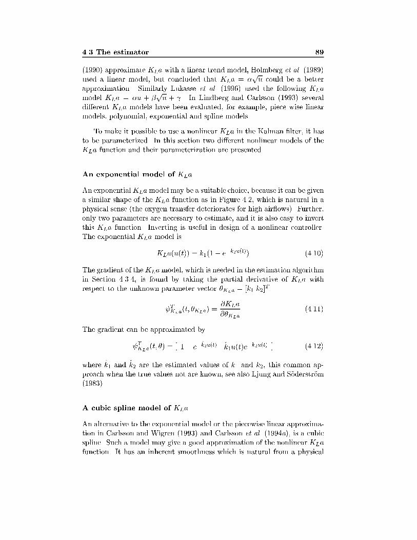
4.3 The estimator 89
(1990) approximate KLa with a linear trend model, Holmberg et al. (1989)used a linear model, but concluded that KLa = �
pu could be a better
approximation. Similarly Lukasse et al. (1996) used the following KLamodel KLa = �u + �
pu + . In Lindberg and Carlsson (1993) several
di�erent KLa models have been evaluated, for example, piece wise linearmodels, polynomial, exponential and spline models.
To make it possible to use a nonlinear KLa in the Kalman �lter, it hasto be parameterized. In this section two di�erent nonlinear models of theKLa function and their parameterization are presented.
An exponential model of KLa
An exponentialKLamodel may be a suitable choice, because it can be givena similar shape of the KLa function as in Figure 4.2, which is natural in aphysical sense (the oxygen transfer deteriorates for high air ows). Further,only two parameters are necessary to estimate, and it is also easy to invertthis KLa function. Inverting is useful in design of a nonlinear controller.The exponential KLa model is
KLa(u(t)) = k1(1� e�k2u(t)) (4.10)
The gradient of theKLamodel, which is needed in the estimation algorithmin Section 4.3.4, is found by taking the partial derivative of KLa withrespect to the unknown parameter vector �KLa = [k1 k2]
T
TKLa(t; �KLa) =
@KLa
@�KLa(4.11)
The gradient can be approximated by
TKLa(t; �) = [ 1� e�k2u(t) k1u(t)e
�k2u(t) ] (4.12)
where k1 and k2 are the estimated values of k1 and k2, this common ap-proach when the true values not are known, see also Ljung and S�oderstr�om(1983).
A cubic spline model of KLa
An alternative to the exponential model or the piecewise linear approxima-tion in Carlsson and Wigren (1993) and Carlsson et al. (1994a), is a cubicspline. Such a model may give a good approximation of the nonlinear KLafunction. It has an inherent smoothness which is natural from a physical

90 Estimation of the DO dynamics
uuu 1 2 3
u
1
3
2
x xx1 2 3
L
u0
K a
θθ
θ
Figure 4.3: A spline approximation of KLa .
point of view. In Figure 4.3 a cubic spline is shown, together with some ofthe parameter de�nitions.
From Dahlquist et al. (1974) it follows that a cubic spline polynomialcan be written in the following form where u is in the interval ui�1 � u < ui
KLa(u)i = mi�i + (1�mi)�i�1
+ ximi(1�mi)[(ki�1 � di)(1�mi)� (ki � di)mi] (4.13)
where �i is de�ned in Figure 4.3 and
xi = ui � ui�1
di =�i � �i�1
xi
mi =u� ui�1
xi; u 2 [ui�1; ui]
i = 1; 2; : : : ; n n = number of grid points � 1
The variables k0; k1; :::; kn are the derivatives of the spline in the grid points.Note that KLa(ui)i = �i.
The linear regression form for the spline model is
KLa(u(t)) = TKLa(t)�KLa (4.14)
�KLa = [�0 : : : �n]T (4.15)
The derivation and de�nition of TKLa(t) is given in Appendix C.
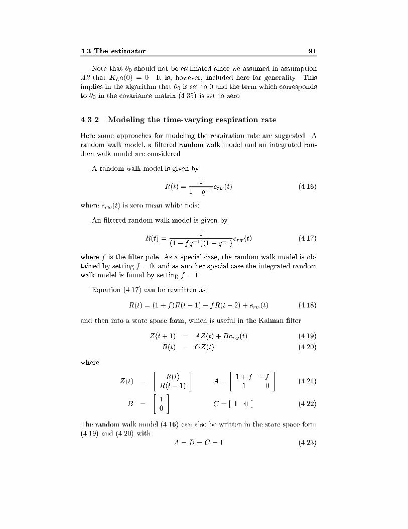
4.3 The estimator 91
Note that �0 should not be estimated since we assumed in assumptionA3 that KLa(0) = 0. It is, however, included here for generality. Thisimplies in the algorithm that �0 is set to 0 and the term which correspondsto �0 in the covariance matrix (4.35) is set to zero.
4.3.2 Modeling the time-varying respiration rate
Here some approaches for modeling the respiration rate are suggested. Arandom walk model, a �ltered random walk model and an integrated ran-dom walk model are considered.
A random walk model is given by
R(t) =1
1� q�1erw(t) (4.16)
where erw(t) is zero mean white noise.
An �ltered random walk model is given by
R(t) =1
(1� fq�1)(1 � q�1)erw(t) (4.17)
where f is the �lter pole. As a special case, the random walk model is ob-tained by setting f = 0, and as another special case the integrated randomwalk model is found by setting f = 1.
Equation (4.17) can be rewritten as
R(t) = (1 + f)R(t� 1)� fR(t� 2) + erw(t) (4.18)
and then into a state space form, which is useful in the Kalman �lter.
Z(t+ 1) = AZ(t) +Berw(t) (4.19)
R(t) = CZ(t) (4.20)
where
Z(t) =
"R(t)
R(t� 1)
#A =
"1 + f �f1 0
#(4.21)
B =
"10
#C = [ 1 0 ] (4.22)
The random walk model (4.16) can also be written in the state space form(4.19) and (4.20) with
A = B = C = 1 (4.23)
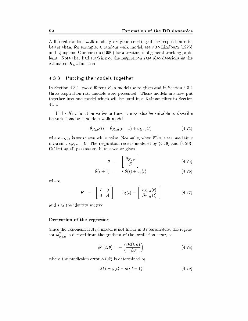
92 Estimation of the DO dynamics
A �ltered random walk model gives good tracking of the respiration rate,better than, for example, a random walk model, see also Lindbom (1995)and Ljung and Gunnarsson (1990) for a treatment of general tracking prob-lems. Note that bad tracking of the respiration rate also deteriorates theestimated KLa function.
4.3.3 Putting the models together
In Section 4.3.1, two di�erent KLa models were given and in Section 4.3.2three respiration rate models were presented. These models are now puttogether into one model which will be used in a Kalman �lter in Section4.3.4.
If the KLa function varies in time, it may also be suitable to describeits variations by a random walk model
�KLa(t) = �KLa(t� 1) + eKLa(t) (4.24)
where eKLa is zero mean white noise. Normally, when KLa is assumed timeinvariant, eKLa = 0. The respiration rate is modeled by (4.19) and (4.20).Collecting all parameters in one vector gives
� =
"�KLa
Z
#(4.25)
�(t+ 1) = F�(t) + e�(t) (4.26)
where
F =
"I 00 A
#e�(t) =
"eKLa(t)Berw(t)
#(4.27)
and I is the identity matrix.
Derivation of the regressor
Since the exponential KLa model is not linear in its parameters, the regres-sor TKLa
is derived from the gradient of the prediction error, as
T (t; �) = ��@"(t; �)
@�
�(4.28)
where the prediction error "(t; �) is determined by
"(t) = y(t)� y(tjt� 1) (4.29)

4.3 The estimator 93
Inserting the predictor y(tjt� 1), which is based on equation (4.9) gives
"(t) = y(t)� y(t� 1) + h�[
Q(t� 1)
V(yin(t� 1)� y(t� 1))
+ dKLa(u(t� 1))(ysat � y(t� 1)) � R(t� 1)]
!(4.30)
Applying (4.28) with the prediction error in (4.30) gives
T (t; �) = h�[(ysat � y(t))@dKLa@�
�@R@�
] (4.31)
which can be written as
T (t; �) = h�[(ysat � y(t)) TKLa(t) �C ] (4.32)
where TKLais given by (4.11) for the exponential model and (C.21) for the
spline model. The C-vector is either given by (4.22) or (4.23) dependingon the model of the respiration rate.
4.3.4 The Kalman �lter
A Kalman �lter interpretation is used to estimate the time-varying respi-ration rate and the nonlinear oxygen transfer function. This approach usesmeasurements of DO and air ow rate to estimate the oxygen transfer func-tion KLa and the respiration rate by a Kalman �lter. A schematic �gureof the estimator is shown in Figure 4.4.'
&
$
%
Kalman �lter
"(t) = y(t)� by(t)�(t) = F �(t� 1) +K(t)"(t)
-y(t)
-u(t)
-dKLa(u)
-R(t)
Figure 4.4: The estimator where KLa and R(t) are estimated from
measurements of DO and air ow rate, see also Carlsson et al. (1994a).
The Kalman �lter equations can, for example, be found in Ljung andS�oderstr�om (1983). These equations together with the parameter modelingfrom Section 4.3.3 give
�(t) = F �(t� 1) +K(t)"(t) (4.33)

94 Estimation of the DO dynamics
K(t) =FP (t� 1) (t)
r2 + T (t)P (t� 1) (t)(4.34)
P (t) = FP (t� 1)F T � FP (t� 1) (t) T (t)P (t� 1)F T
r2 + T (t)P (t� 1) (t)+R1(4.35)
where "(t) is de�ned in (4.29), � in (4.25), (t) in (4.32), and the choice ofR1 in (4.37) for a random walk and (4.38) for a �ltered random walk, andr2 = 1.
In the predictor, the parameters y(t), yin(t), u(t) and Q(t) are mea-sured, V and ysat are assumed known and R(t) and �KLa are estimated.The parameter h� is derived according to (4.7) with an estimated value ofKLa(u).
Choice of R1 and r2
The covariance matrix R1 is given by
R1 = Ee�(t)e�(t)T =
"Ee2KLa
0
0 BBTEe2rw
#(4.36)
and describes how fast the di�erent components in � are expected to vary.Usually Ee2KLa
and Ee2rw are not known. The variance of the measurementnoise w(t) is denoted by r2. It is possible to rewrite (4.35) so that R1 isreplaced by R1=r2 and r2 by 1. Then only R1 is used as a design parameter.This is reasonable, since in most cases neither R1 nor r2 are known.
Setting R1 = 0 implies no tracking capability, since K(t) then goes tozero when t ! 1. Hence to be able to track time-varying parameters itis necessary to set R1 > 0. The magnitude of R1 should re ect the truevariations of the time varying parameters and has in general to be triedout.
In the dissolved oxygen dynamics, the respiration rate is time-varyingand the KLa function is assumed to be a very slowly changing (or time-invariant) nonlinearity of the air ow rate. The covariance matrix R1 thenbecomes
R1 =
264 1 0 00 1 00 0 2
375 (4.37)
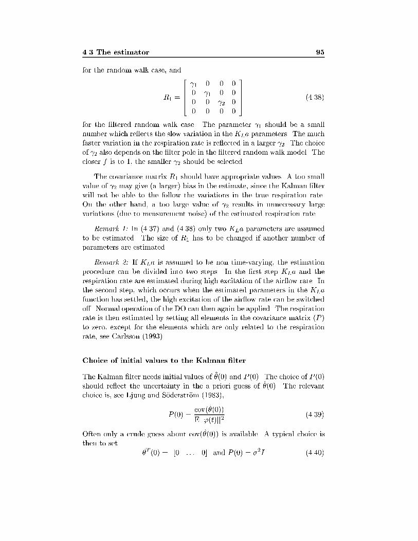
4.3 The estimator 95
for the random walk case, and
R1 =
26664 1 0 0 00 1 0 00 0 2 00 0 0 0
37775 (4.38)
for the �ltered random walk case. The parameter 1 should be a smallnumber which re ects the slow variation in the KLa parameters. The muchfaster variation in the respiration rate is re ected in a larger 2. The choiceof 2 also depends on the �lter pole in the �ltered random walk model. Thecloser f is to 1, the smaller 2 should be selected.
The covariance matrix R1 should have appropriate values. A too smallvalue of 2 may give (a larger) bias in the estimate, since the Kalman �lterwill not be able to the follow the variations in the true respiration rate.On the other hand, a too large value of 2 results in unnecessary largevariations (due to measurement noise) of the estimated respiration rate.
Remark 1: In (4.37) and (4.38) only two KLa parameters are assumedto be estimated. The size of R1 has to be changed if another number ofparameters are estimated.
Remark 2: If KLa is assumed to be non time-varying, the estimationprocedure can be divided into two steps. In the �rst step KLa and therespiration rate are estimated during high excitation of the air ow rate. Inthe second step, which occurs when the estimated parameters in the KLafunction has settled, the high excitation of the air ow rate can be switchedo�. Normal operation of the DO can then again be applied. The respirationrate is then estimated by setting all elements in the covariance matrix (P )to zero, except for the elements which are only related to the respirationrate, see Carlsson (1993)
Choice of initial values to the Kalman �lter
The Kalman �lter needs initial values of �(0) and P (0). The choice of P (0)should re ect the uncertainty in the a priori guess of �(0). The relevantchoice is, see Ljung and S�oderstr�om (1983),
P (0) =cov(�(0))
Ejj'(t)jj2 (4.39)
Often only a crude guess about cov(�(0)) is available. A typical choice isthen to set
�T (0) = [0 : : : 0] and P (0) = �2I (4.40)

96 Estimation of the DO dynamics
where I is the identity matrix, and �2 should be chosen large.
Remark: A very important practical issue when using any kind of re-cursive algorithm is the initialization. If one uses a large � at t = 0 and theregressor is �lled with zeros, it is very likely that the parameters take somelarge steps in a wrong direction which they often never recover from. Aremedy is to wait with the updating until the regressor is �lled with data.
4.3.5 An alternative approach of estimating KLa
A possible alternative approach to the Kalman �lter approach discussedabove is to �rst di�erentiate the model and treat the di�erentiated res-piration rate as white noise. Di�erentiating is a well known method insystem identi�cation to be applied to systems with non-zero means, see,e.g., S�oderstr�om and Stoica (1989).
Since the di�erentiated respiration rate is treated as a white noise, fewerparameters have to be estimated than in the previously mentioned ap-proaches where the respiration rate also was estimated. Estimating fewerparameters usually implies higher accuracy of the remaining parameters.The value of the respiration rate is not lost by the use of this approach, itcan still be determined by using equation (4.9) together with the estimatedKLa.
Using (4.9) (neglecting the noise w(t)) and calculating y(t + 1) � y(t)gives
y(t+ 1)� y(t) = y(t)� y(t� 1) + h�[Q(t)
V(yin(t)� y(t))
�Q(t� 1)
V(yin(t� 1)� y(t� 1)) +KLa(u(t))(ysat � y(t))
�KLa(u(t� 1))(ysat � y(t� 1))� (R(t)�R(t� 1))] (4.41)
Assuming that the respiration rate can be modeled by
R(t) =1
1� q�1erw(t) (4.42)
where the noise erw is assumed to be zero mean white noise, gives
R(t)�R(t� 1) = erw(t) (4.43)
Inserting (4.43) in (4.41) gives the predictor
y(t+ 1jt) = 2y(t)� y(t� 1) + h�[Q(t)
V(yin(t)� y(t))

4.4 Estimation utilizing a slow DO sensor 97
� Q(t� 1)
V(yin(t� 1)� y(t� 1)) +KLa(u(t))(ysat � y(t� 1))
� KLa(u(t� 1))(ysat � y(t� 1))] (4.44)
The gradient of (4.44) becomes
T (t) = h[(ysat � y(t� 1)) TKLa(t� 1)� (ysat � y(t� 2)) TKLa
(t� 2)] (4.45)
where TKLa(t) is de�ned in (4.11). Note that this predictor is di�erent as
compared to the previous one.
This method works very well when no measurement noise exists, evenbetter than the other methods. Its performance deteriorates, however,fast (faster than it does for the other methods) when measurement noiseis added. A possible explaination could be that di�erentiation ampli�esnoise.
4.4 Estimation utilizing a slow DO sensor
When estimating the respiration rate and oxygen transfer function frommeasurements of DO and air ow rates, it is necessary that a high excitationin the air ow rate is used. A high excitation in air ow rate implies rapidchanges in DO. If the DO sensor is not fast, the estimates will be biased. Inthis section a �ltering procedure, developed by Ahl�en and Sternad (1989),is applied to reduce the in uence of the DO sensor dynamics. The �lteredDO measurements are then used for estimating the respiration rate and theoxygen transfer function.
4.4.1 Simple illustration of the problem
Assume for simplicity that Q(t) = u(t) = 0. Inserting this in (4.4) givesthe respiration rate
R(t) = �dydt
(4.46)
The respiration rate can hence be estimated from the slope of the sensoroutput. If the DO sensor is slow, how will then the estimated respira-tion rate be a�ected, when using (4.46)? An example will illustrate thisquestion.
Let the DO sensor have a step response as shown in Figure 4.5. Thetrue DO is changed from zero to one mg/l at time t = 0.
If the DO is 2 mg/l at t = 0, applying the respiration rate in the lowerplot of Figure 4.6 then gives the DO shown in the upper plot in the same

98 Estimation of the DO dynamics
0 20 40 60 80 100 120 140 160 180 2000
0.2
0.4
0.6
0.8
1
time [s]
mg/
l
Step response of a DO sensor
Figure 4.5: Step response of a DO sensor.
�gure. We can see that DO sensor output is slower than the true DO. Usingthe derivative of the sensor output as an estimate of the respiration rate willhence not give a correct estimate. It takes time before a reliable estimate ofthe respiration rate is achieved. If there is a step change in the respirationrate, the settling-time to obtain a correct estimate will then be as long asthe settling-time for the DO sensor. The estimate of the respiration rate is�ltered by the sensor dynamics.
When the air ow rate is highly excited, which it should be to give goodestimates of the respiration rate and KLa, the DO sensor output will notfollow the true DO and the estimates will be biased.
4.4.2 Filtering the DO measurements
Assume that the DO is measured by a sensor. Obviously, what is availablefor data processing is the output from the sensor (denoted ys(t) below).By �ltering the DO measurements it is possible to reduce in uence of thesensor dynamics. This is utilized by using a �xed lag smoother. A blockdiagram of the sensor, the input model and the �lter is shown in Figure4.7.
We would like to �nd a �lter, which based on the measurements of thesensor output (ys(t)) gives the actual DO in the activated sludge process.The problem is to �nd a �lter which minimizes the mean square errorbetween the true DO and the �ltered DO, i.e. we want to minimize
E(y(t)� y(tjt�m))2 (4.47)
where y(tjt � m) denotes a prediction of y(t) based on data up to timet�m. The user choice m determines whether we have a predictor (m > 0),
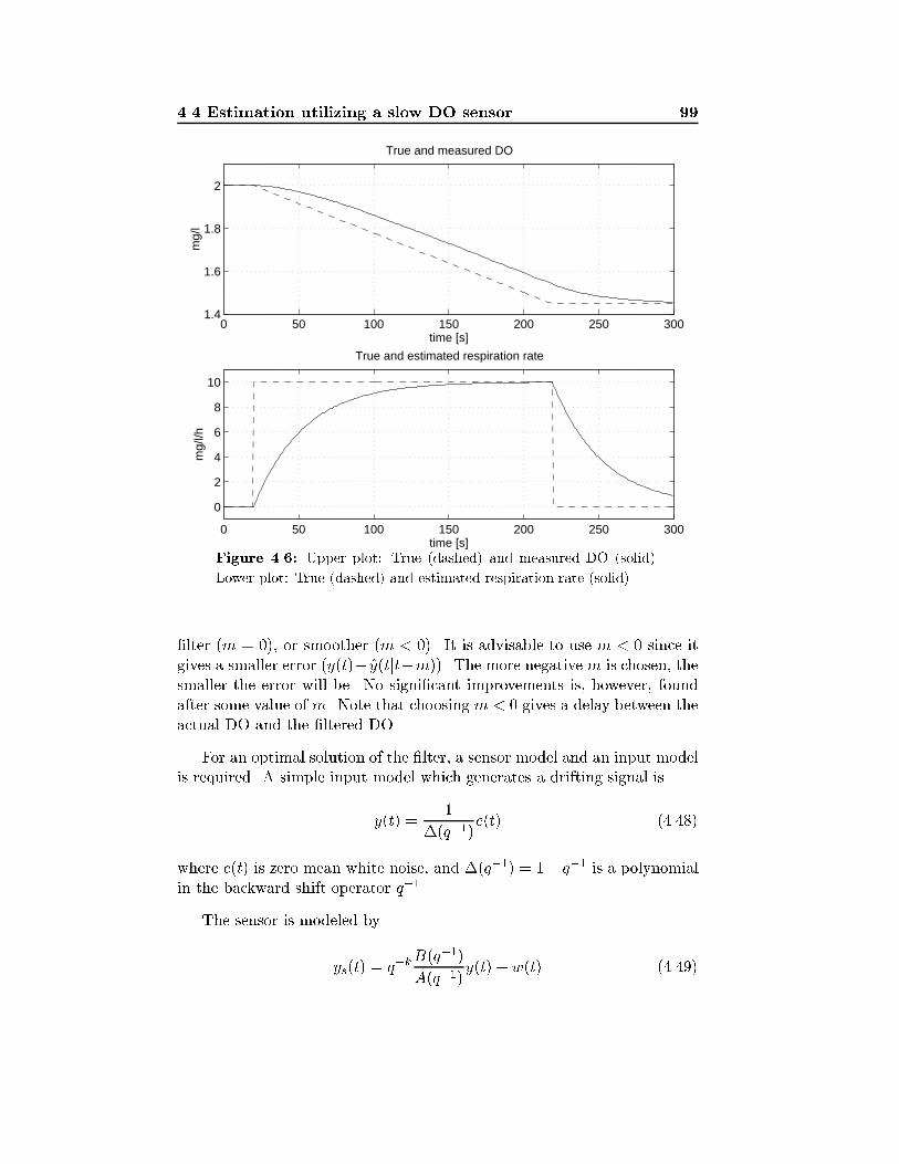
4.4 Estimation utilizing a slow DO sensor 99
0 50 100 150 200 250 3001.4
1.6
1.8
2
True and measured DO
time [s]
mg/
l
0 50 100 150 200 250 300
0
2
4
6
8
10
True and estimated respiration rate
time [s]
mg/
l/h
Figure 4.6: Upper plot: True (dashed) and measured DO (solid).
Lower plot: True (dashed) and estimated respiration rate (solid).
�lter (m = 0), or smoother (m < 0). It is advisable to use m < 0 since itgives a smaller error (y(t)� y(tjt�m)). The more negative m is chosen, thesmaller the error will be. No signi�cant improvements is, however, foundafter some value of m. Note that choosing m < 0 gives a delay between theactual DO and the �ltered DO.
For an optimal solution of the �lter, a sensor model and an input modelis required. A simple input model which generates a drifting signal is
y(t) =1
�(q�1)e(t) (4.48)
where e(t) is zero mean white noise, and �(q�1) = 1� q�1 is a polynomialin the backward shift operator q�1.
The sensor is modeled by
ys(t) = q�kB(q�1)
A(q�1)y(t) + w(t) (4.49)
100 Estimation of the DO dynamics
����1� q�k B
A q�mQR
- - - - -?
SensorDO
�+
+
Inputmodel Filter
e(t) y(t) ys(t) y(tjt�m)
w(t)
Figure 4.7: Block diagram of the input signal, the sensor model and
the �lter.
In (4.49) k is a time delay, A(q�1) and B(q�1) are polynomials and w(t) iszero mean white measurement noise.
The problem of minimizing (4.47) is an LQ problem, which either couldbe solved by a Kalman �lter approach or by a polynomial approach. Thelatter method is applied here.
The �lter which minimizes (4.47) is given by
y(tjt�m) = q�mQ(q�1)
R(q�1)ys(t) (4.50)
where the Q(q�1) and R(q�1) polynomials are found by solving the follow-ing design equations, see Ahl�en and Sternad (1989)
r��� = BB� + �A�A��� (4.51)
zm+kB� = r��Q1 + z�L� (4.52)
Q = Q1A (4.53)
R = � (4.54)
In (4.51) { (4.54) and in the following the argument (q�1) is left out forsimplicity. Conjugate polynomials (denoted by �) are used in (4.51) and(4.52). A conjugate polynomial is de�ned as follows. Consider a generalpolynomial P = p0 + p1q
�1 + � � � + pnP q�nP . The conjugate polynomial
is then de�ned by P� = p0 + p1q + � � � + pnP qnP . The polynomial � is
a stable (the roots of � are inside the unit circle) and monic (the �rstcoe�cient in the polynomial is 1) polynomial. The polynomial L is anauxiliary polynomial, and � = Ew2=Ee2 is the noise to signal ratio, whichis normally used as user design parameter.
4.4 Estimation utilizing a slow DO sensor 101
The degrees of the polynomials in the design equations (4.51){(4.54)are given by:
n� =
(nB if � = 0maxfnB; nA+ 1g if � > 0
(4.55)
nQ1 = maxf�m� k; 0g (4.56)
nL = maxfnB +m+ k; n�g � 1 (4.57)
where nB denotes the degree of the B polynomial, etc.
Remark 1: The presented approach may, for example, also be of interestfor DO sensors used in respirometers, see e.g. Spanjers and Olsson (1992).
Remark 2: E�cient numerical methods exist for solving the spectralfactorization (4.51), which can only be solved analytically for degrees of �less than 3.
Remark 3: It is possible to derive a �lter for a more general case wherethe measurement noise w(t) is colored and the input model is more general,see further Ahl�en and Sternad (1989).
4.4.3 Determination of A, B, k and �
The sensor model, i.e. the A and B polynomials and time delay k, can bedetermined by a least squares method, where suitable polynomial degreesand time delay have to be tried out, see e.g. S�oderstr�om and Stoica (1989).Necessary data for estimating the sensor dynamics can be achieved by mov-ing the the DO sensor between waters with di�erent DO and register thesensor response.
The parameter � is probably easiest to �nd by trial and error. A small� gives a noisy result and a large � gives a slow response to changes inDO. When estimating the respiration rate from the DO measurements,simulations have indicated that it is better to choose a too small than atoo large �.
4.4.4 An example
To illustrate the procedure outlined above, an example is given. The dy-namics of the sensor in this example corresponds to the model obtainedfor the DO sensor at the pilot plant in Uppsala. For a sampling intervalof 10s the following parameters were identi�ed from the data given in theexperiment shown in Figure 4.8 using a least squares method (ARX model
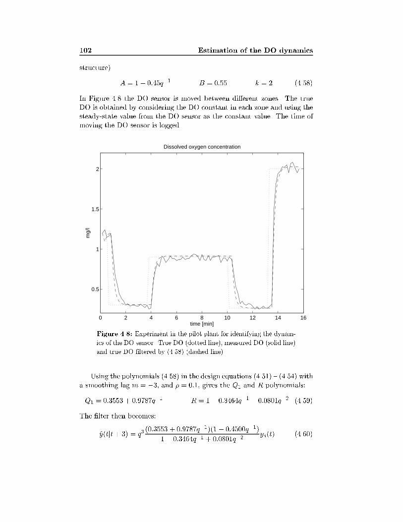
102 Estimation of the DO dynamics
structure)
A = 1� 0:45q�1 B = 0:55 k = 2 (4.58)
In Figure 4.8 the DO sensor is moved between di�erent zones. The trueDO is obtained by considering the DO constant in each zone and using thesteady-state value from the DO sensor as the constant value. The time ofmoving the DO sensor is logged.
0 2 4 6 8 10 12 14 16
0.5
1
1.5
2
time [min]
mg/
l
Dissolved oxygen concentration
Figure 4.8: Experiment in the pilot plant for identifying the dynam-
ics of the DO sensor. True DO (dotted line), measured DO (solid line)
and true DO �ltered by (4.58) (dashed line).
Using the polynomials (4.58) in the design equations (4.51) { (4.54) witha smoothing lag m = �3, and � = 0:1, gives the Q1 and R polynomials:
Q1 = 0:3553 + 0:9787q�1 R = 1� 0:3464q�1 + 0:0801q�2 (4.59)
The �lter then becomes:
y(tjt+ 3) = q3(0:3553 + 0:9787q�1)(1 � 0:4500q�1)
1� 0:3464q�1 + 0:0801q�2ys(t) (4.60)
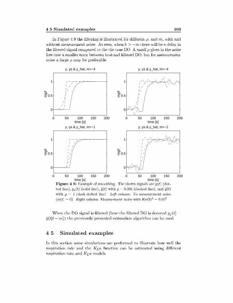
4.5 Simulated examples 103
In Figure 4.9 the �ltering is illustrated for di�erent �, and m, with andwithout measurement noise. As seen, when k > �m there will be a delay inthe �ltered signal compared to the the true DO. A small � gives in the noisefree case a smaller error between true and �ltered DO, but for measurementnoise a large � may be preferable.
0 50 100 150 200
0
0.5
1
y, ys & y_hat, m=−4
time [s]
mg/
l
0 50 100 150 200
0
0.5
1
y, ys & y_hat, m=−4
time [s]m
g/l
0 50 100 150 200
0
0.5
1
y, ys & y_hat, m=−1
time [s]
mg/
l
0 50 100 150 200
0
0.5
1
y, ys & y_hat, m=−1
time [s]
mg/
l
Figure 4.9: Example of smoothing. The shown signals are y(t) (dot-
ted line), ys(t) (solid line), y(t) with � = 0:001 (dashed line), and y(t)
with � = 1 (dash-dotted line). Left column: No measurement noise
(w(t) = 0). Right column: Measurement noise with Ew(t)2 = 0:052.
When the DO signal is �ltered (here the �ltered DO is denoted yf (t) =y(tjt�m)) the previously presented estimation algorithm can be used.
4.5 Simulated examples
In this section some simulations are performed to illustrate how well therespiration rate and the KLa function can be estimated using di�erentrespiration rate and KLa models.

104 Estimation of the DO dynamics
4.5.1 Simulation setup
In the simulations, a setup is used which approximately corresponds to the�rst aerobic zone in the pilot plant at Kungs�angsverket. In the pilot plantthe air ow rate can not be measured. Instead the valve opening is used, seeSection 4.6.1 for more details. If the air ow rate or valve opening is useddoes not change the estimation algorithm, the general idea is the same.
The system used for generating the data is simulated by
y(t+1) = y(t)+h�[Q(t)
V(yin(t)�y(t))+KLa(u(t))(ysat�y(t))�R(t)] (4.61)
where
� The wastewater ow, Q = 1000 l/h
� The volume of the zone, V = 630 l
� The saturated DO, ysat = 10 mg/l
� The in uent DO, yin(t) = 0 mg/l
� The oxygen transfer function KLa(u) = 5 arctan( 20u1000 ) h�1
� The respiration rate R(t) = 20 + 15 sin(6t) mg/l/h.
� h�(t) = 1A(t) (e
A(t)h � 1), A(t) = �(KLa(u(t)) +Q(t)V
)
� The sampling period, h = 1=360 h, (10s)
� Zero mean white measurement noise with standard deviation 0.1 hasbeen added to the output.
In the estimation algorithm the following setup is used:
� Correct values were used for Q=V , yin(t) and ysat.
� In the covariance matrix R1, 1 is set to 0, and 2 is given by:
* 2 = 100 for the random walk model.
* 2 = 0:05 for the integrated random walk model.
* 2 = 0:2 for the �ltered random walk model where f = 0:97.
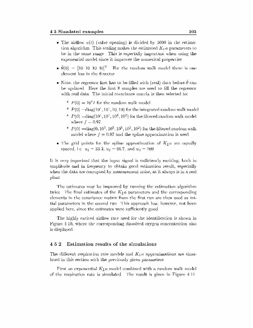
4.5 Simulated examples 105
� The air ow u(t) (valve opening) is divided by 1000 in the estima-tion algorithm. This scaling makes the estimated KLa parameters tobe in the same range. This is especially important when using theexponential model since it improves the numerical properties.
� �(0) = [10 10 10 10]T . For the random walk model there is oneelement less in the �-vector.
� Note, the regressor �rst has to be �lled with (real) data before � canbe updated. Here the �rst 8 samples are used to �ll the regressorwith real data. The initial covariance matrix is then selected to:
* P (0) = 104I for the random walk model.
* P (0) =diag(104; 104; 10; 10) for the integrated random walk model.
* P (0) =diag(104; 104; 102; 102) for the �ltered random walk modelwhere f = 0:97.
* P (0) =diag(0; 105; 105; 105; 102; 102) for the �ltered random walkmodel where f = 0:97 and the spline approximation is used.
� The grid points for the spline approximation of KLa are equallyspaced, i.e. u1 = 33:3, u2 = 66:7, and u3 = 100.
It is very important that the input signal is su�ciently exciting, both inamplitude and in frequency to obtain good estimation result, especiallywhen the data are corrupted by measurement noise, as it always is in a realplant.
The estimates may be improved by running the estimation algorithmtwice. The �nal estimates of the KLa parameters and the correspondingelements in the covariance matrix from the �rst run are then used as ini-tial parameters in the second run. This approach has, however, not beenapplied here, since the estimates were su�ciently good.
The highly excited air ow rate used for the identi�cation is shown inFigure 4.10, where the corresponding dissolved oxygen concentration alsois displayed.
4.5.2 Estimation results of the simulations
The di�erent respiration rate models and KLa approximations are simu-lated in this section with the previously given parameters.
First an exponential KLa model combined with a random walk modelof the respiration rate is simulated. The result is given in Figure 4.11.
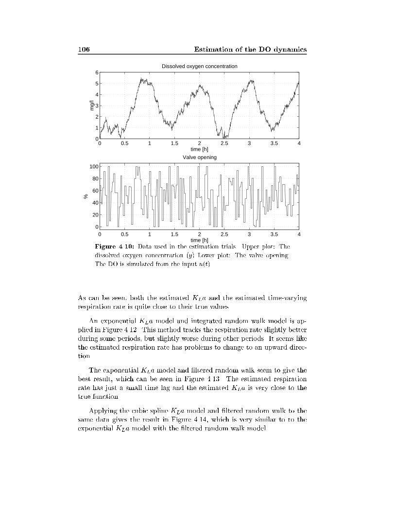
106 Estimation of the DO dynamics
0 0.5 1 1.5 2 2.5 3 3.5 40
1
2
3
4
5
6
time [h]
mg/
l
Dissolved oxygen concentration
0 0.5 1 1.5 2 2.5 3 3.5 40
20
40
60
80
100
time [h]
%
Valve opening
Figure 4.10: Data used in the estimation trials. Upper plot: The
dissolved oxygen concentration (y) Lower plot: The valve opening.
The DO is simulated from the input u(t).
As can be seen, both the estimated KLa and the estimated time-varyingrespiration rate is quite close to their true values.
An exponential KLa model and integrated random walk model is ap-plied in Figure 4.12. This method tracks the respiration rate slightly betterduring some periods, but slightly worse during other periods. It seems likethe estimated respiration rate has problems to change to an upward direc-tion.
The exponential KLa model and �ltered random walk seem to give thebest result, which can be seen in Figure 4.13. The estimated respirationrate has just a small time lag and the estimated KLa is very close to thetrue function.
Applying the cubic spline KLa model and �ltered random walk to thesame data gives the result in Figure 4.14, which is very similar to to theexponential KLa model with the �ltered random walk model.

4.5 Simulated examples 107
0 1 2 3 40
5
10
15
20Estimated Kla−parameters
time [h]0 50 100
0
1
2
3
4
5
6
1/h
True & estimated Kla function
Valve opening [%]
0 0.5 1 1.5 2 2.5 3 3.5 4
0
10
20
30
40True and estimated respiration rate
time [h]
mg/
l/h
Figure 4.11: A simulation with an exponentialKLamodel and a ran-
dom walk model of the respiration rate. Upper left plot: The settling
of the parameters in the exponential KLa model. Upper right plot:
True KLa (solid line) and estimated KLa (dashed line) at the �nal
time. Lower plot: True (smooth line) and and estimated respiration
rate.
As a conclusion one can say that the di�erent suggested methods do notshow any large di�erences. What is most important is the initialization ofthe covariance matrix P and choice of the R1 matrix. A �ltered randomwalk model seems, however, to be to prefer. A spline or exponential modelgive almost identical results. Since the exponential model is simpler wemight as well use that one.
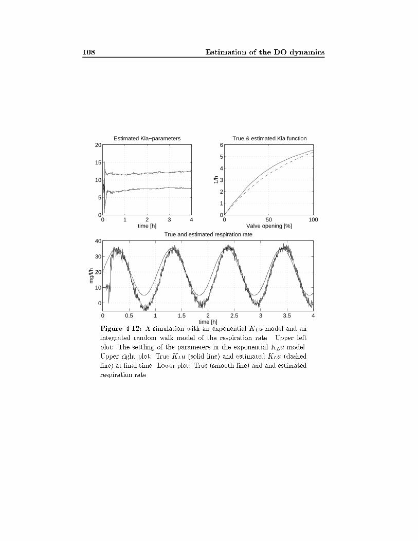
108 Estimation of the DO dynamics
0 1 2 3 40
5
10
15
20Estimated Kla−parameters
time [h]0 50 100
0
1
2
3
4
5
6
1/h
True & estimated Kla function
Valve opening [%]
0 0.5 1 1.5 2 2.5 3 3.5 4
0
10
20
30
40True and estimated respiration rate
time [h]
mg/
l/h
Figure 4.12: A simulation with an exponential KLa model and an
integrated random walk model of the respiration rate. Upper left
plot: The settling of the parameters in the exponential KLa model.
Upper right plot: True KLa (solid line) and estimated KLa (dashed
line) at �nal time. Lower plot: True (smooth line) and and estimated
respiration rate.
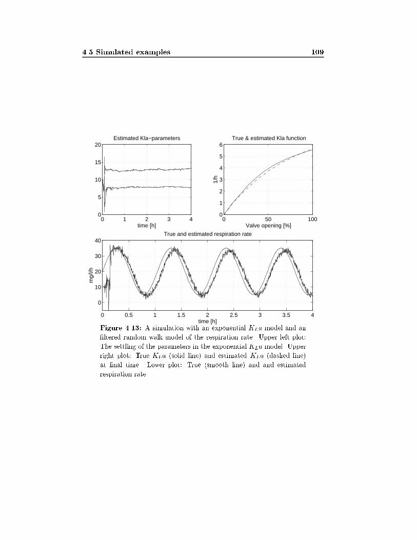
4.5 Simulated examples 109
0 1 2 3 40
5
10
15
20Estimated Kla−parameters
time [h]0 50 100
0
1
2
3
4
5
6
1/h
True & estimated Kla function
Valve opening [%]
0 0.5 1 1.5 2 2.5 3 3.5 4
0
10
20
30
40True and estimated respiration rate
time [h]
mg/
l/h
Figure 4.13: A simulation with an exponential KLa model and an
�ltered random walk model of the respiration rate. Upper left plot:
The settling of the parameters in the exponential KLa model. Upper
right plot: True KLa (solid line) and estimated KLa (dashed line)
at �nal time. Lower plot: True (smooth line) and and estimated
respiration rate.
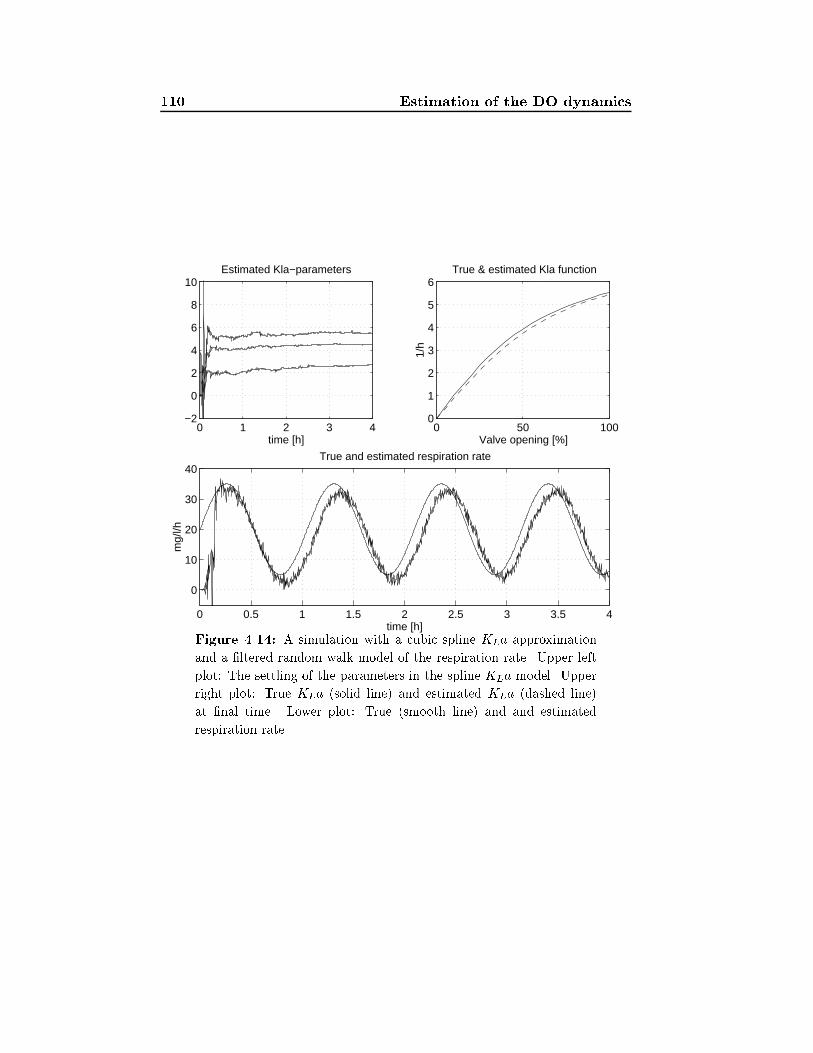
110 Estimation of the DO dynamics
0 1 2 3 4−2
0
2
4
6
8
10Estimated Kla−parameters
time [h]0 50 100
0
1
2
3
4
5
6
1/h
True & estimated Kla function
Valve opening [%]
0 0.5 1 1.5 2 2.5 3 3.5 4
0
10
20
30
40True and estimated respiration rate
time [h]
mg/
l/h
Figure 4.14: A simulation with a cubic spline KLa approximation
and a �ltered random walk model of the respiration rate. Upper left
plot: The settling of the parameters in the spline KLa model. Upper
right plot: True KLa (solid line) and estimated KLa (dashed line)
at �nal time. Lower plot: True (smooth line) and and estimated
respiration rate.
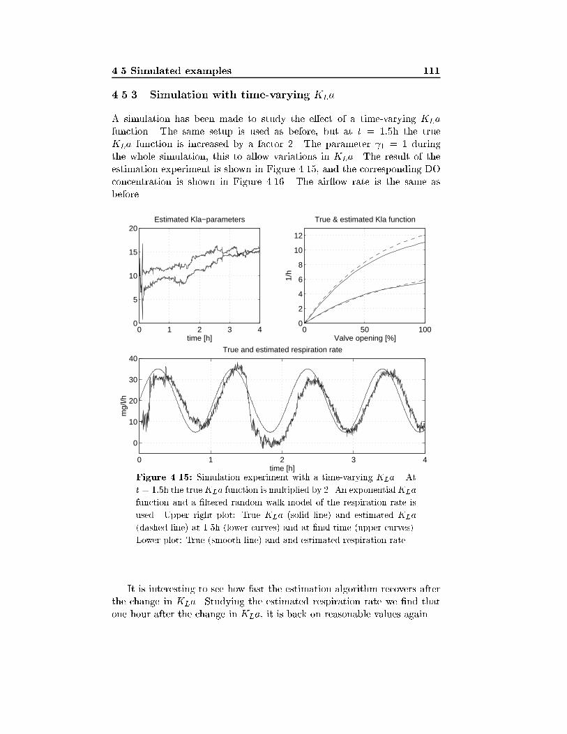
4.5 Simulated examples 111
4.5.3 Simulation with time-varying KLa
A simulation has been made to study the e�ect of a time-varying KLafunction. The same setup is used as before, but at t = 1:5h the trueKLa function is increased by a factor 2. The parameter 1 = 1 duringthe whole simulation, this to allow variations in KLa. The result of theestimation experiment is shown in Figure 4.15, and the corresponding DOconcentration is shown in Figure 4.16. The air ow rate is the same asbefore.
0 1 2 3 40
5
10
15
20Estimated Kla−parameters
time [h]0 50 100
0
2
4
6
8
10
12
Valve opening [%]
1/h
True & estimated Kla function
0 1 2 3 4
0
10
20
30
40
time [h]
mg/
l/h
True and estimated respiration rate
Figure 4.15: Simulation experiment with a time-varying KLa . At
t = 1:5h the trueKLa function is multiplied by 2. An exponentialKLa
function and a �ltered random walk model of the respiration rate is
used. Upper right plot: True KLa (solid line) and estimated KLa
(dashed line) at 1.5h (lower curves) and at �nal time (upper curves).
Lower plot: True (smooth line) and and estimated respiration rate.
It is interesting to see how fast the estimation algorithm recovers afterthe change in KLa. Studying the estimated respiration rate we �nd thatone hour after the change in KLa, it is back on reasonable values again.
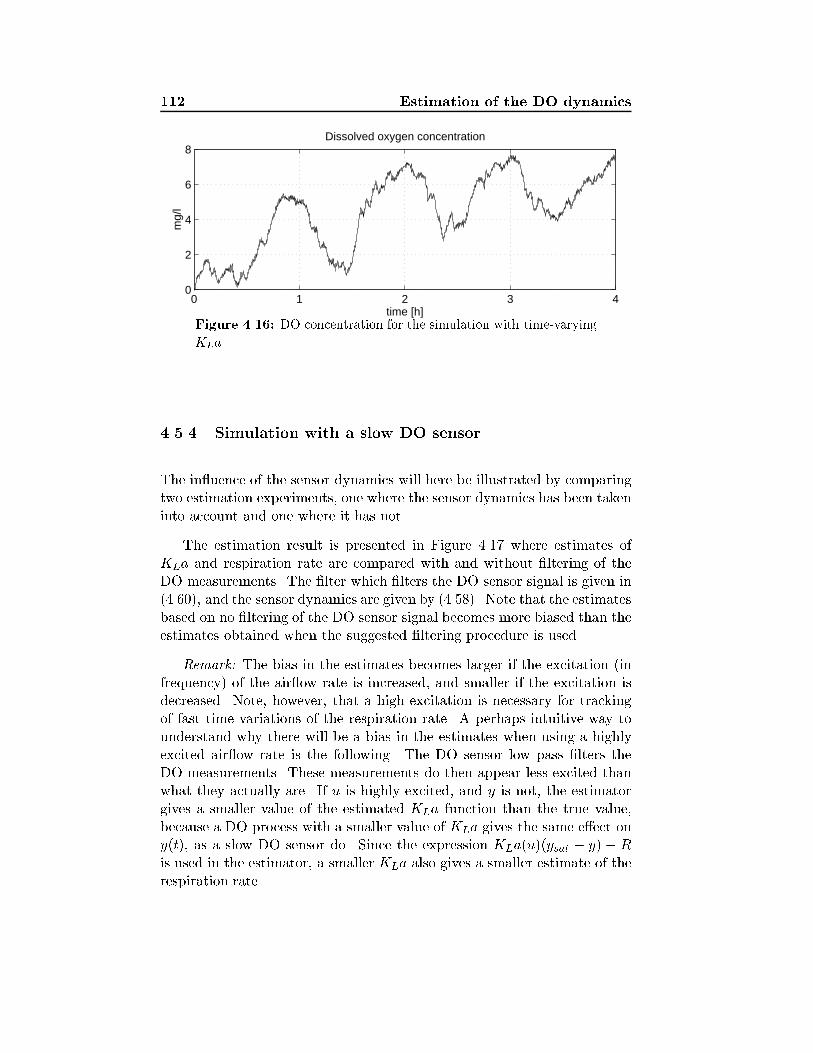
112 Estimation of the DO dynamics
0 1 2 3 40
2
4
6
8
time [h]
mg/
l
Dissolved oxygen concentration
Figure 4.16: DO concentration for the simulation with time-varying
KLa.
4.5.4 Simulation with a slow DO sensor
The in uence of the sensor dynamics will here be illustrated by comparingtwo estimation experiments, one where the sensor dynamics has been takeninto account and one where it has not.
The estimation result is presented in Figure 4.17 where estimates ofKLa and respiration rate are compared with and without �ltering of theDO measurements. The �lter which �lters the DO sensor signal is given in(4.60), and the sensor dynamics are given by (4.58). Note that the estimatesbased on no �ltering of the DO sensor signal becomes more biased than theestimates obtained when the suggested �ltering procedure is used.
Remark: The bias in the estimates becomes larger if the excitation (infrequency) of the air ow rate is increased, and smaller if the excitation isdecreased. Note, however, that a high excitation is necessary for trackingof fast time variations of the respiration rate. A perhaps intuitive way tounderstand why there will be a bias in the estimates when using a highlyexcited air ow rate is the following. The DO sensor low pass �lters theDO measurements. These measurements do then appear less excited thanwhat they actually are. If u is highly excited, and y is not, the estimatorgives a smaller value of the estimated KLa function than the true value,because a DO process with a smaller value of KLa gives the same e�ect ony(t), as a slow DO sensor do. Since the expression KLa(u)(ysat � y) � Ris used in the estimator, a smaller KLa also gives a smaller estimate of therespiration rate.
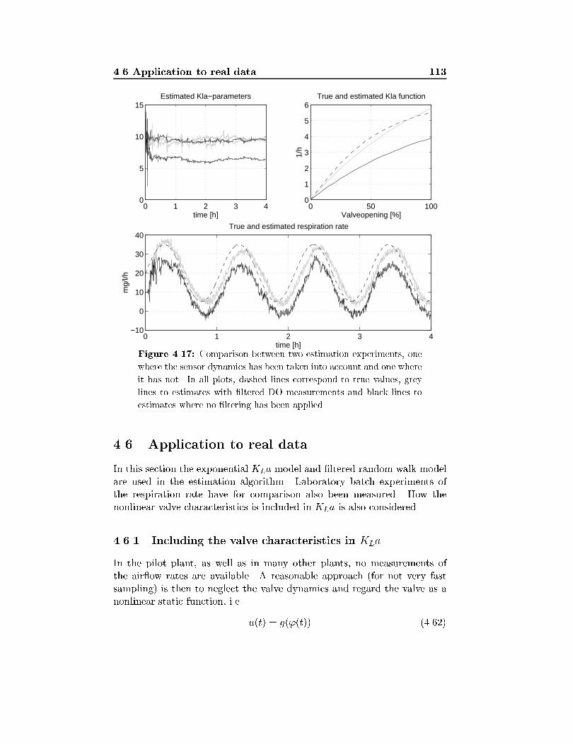
4.6 Application to real data 113
0 1 2 3 40
5
10
15
time [h]
Estimated Kla−parameters
0 1 2 3 4−10
0
10
20
30
40
time [h]
mg/
l/h
True and estimated respiration rate
0 50 1000
1
2
3
4
5
6
Valveopening [%]
1/h
True and estimated Kla function
Figure 4.17: Comparison between two estimation experiments, one
where the sensor dynamics has been taken into account and one where
it has not. In all plots, dashed lines correspond to true values, grey
lines to estimates with �ltered DO measurements and black lines to
estimates where no �ltering has been applied.
4.6 Application to real data
In this section the exponential KLa model and �ltered random walk modelare used in the estimation algorithm. Laboratory batch experiments ofthe respiration rate have for comparison also been measured. How thenonlinear valve characteristics is included in KLa is also considered.
4.6.1 Including the valve characteristics in KLa
In the pilot plant, as well as in many other plants, no measurements ofthe air ow rates are available. A reasonable approach (for not very fastsampling) is then to neglect the valve dynamics and regard the valve as anonlinear static function, i.e.
u(t) = g('(t)) (4.62)

114 Estimation of the DO dynamics
where u(t) is the air ow rate, g is a static function and '(t) is the valveopening which is measurable.
Including (4.62) in the KLa model gives
y(t+1) = y(t)+h[Q(t)
V(yin(t)�y(t))+KLa
g('(t))(ysat�y(t))�R(t)]+w(t)(4.63)
where
KLag('(t)) = KLa(g('(t))) (4.64)
The approach presented in Section 4.3 can now be applied by replacingKLa with KLa
g.
4.6.2 A practical experiment
Several experiments have been performed to estimate KLa and the respira-tion rate, both in the pilot plant and in the full scale plant, see e.g. Carlssonand Wigren (1993), Carlsson (1993), Carlsson et al. (1994a) and Lindbergand Carlsson (1996c). Here, one of the experiment in the pilot plant atUppsala wastewater treatment plant is presented.
In the experiment �ltering of the DO measurement is applied. Thesetup of the DO �lter and the estimator is identical to the setup used inthe simulation study presented in Section 4.5.4. The respiration rate hasfor comparison also been measured in laboratory batch experiments, seeSection 4.6.3 for a further explanation.
In Figure 4.18 the estimated and measured respiration rate are pre-sented. Note that the di�erent methods almost obtain the same values ofthe respiration rate.
Remark 1: If the DO measurement is not �ltered, the estimated respi-ration rate became lower, here � 3 mg/l/h.
Remark 2: Practical experiment have shown that the estimated res-piration rate depends on the air ow rate and/or DO. This was detectedin sequential experiments with identical excitation sequences where a cor-relation between the estimated respiration rates was detected. The truerespiration rate probably depends on the DO since, for example, DO=0gives R(t) � 0.
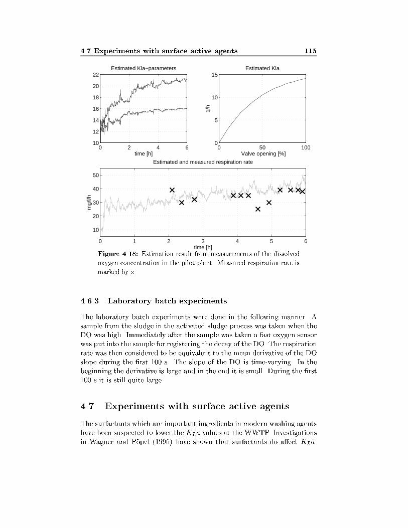
4.7 Experiments with surface active agents 115
0 2 4 610
12
14
16
18
20
22
time [h]
Estimated Kla−parameters
0 50 1000
5
10
15
Valve opening [%]
1/h
Estimated Kla
0 1 2 3 4 5 6
10
20
30
40
50
time [h]
mg/
l/h
Estimated and measured respiration rate
Figure 4.18: Estimation result from measurements of the dissolved
oxygen concentration in the pilot plant. Measured respiration rate is
marked by x.
4.6.3 Laboratory batch experiments
The laboratory batch experiments were done in the following manner. Asample from the sludge in the activated sludge process was taken when theDO was high. Immediately after the sample was taken a fast oxygen sensorwas put into the sample for registering the decay of the DO. The respirationrate was then considered to be equivalent to the mean derivative of the DOslope during the �rst 100 s. The slope of the DO is time-varying. In thebeginning the derivative is large and in the end it is small. During the �rst100 s it is still quite large.
4.7 Experiments with surface active agents
The surfactants which are important ingredients in modern washing agentshave been suspected to lower the KLa values at the WWTP. Investigationsin Wagner and P�opel (1996) have shown that surfactants do a�ect KLa.
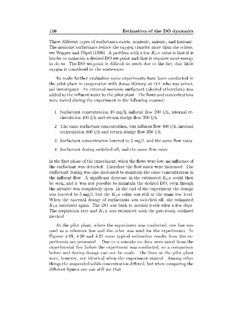
116 Estimation of the DO dynamics
Three di�erent types of surfactants exists, nonionic, anionic, and kationic.The nonionic surfactants reduce the oxygen transfer more than the others,see Wagner and P�opel (1996). A problem with a low KLa value is that it isharder to maintain a desired DO set-point and that it requires more energyto do so. The DO set-point is di�cult to reach due to the fact that littleoxygen is transfered to the wastewater.
To make further evaluation some experiments have been conducted inthe pilot plant in cooperation with Jonas R�ottorp at IVL who was princi-pal investigator. An external nonionic surfactant (alcohol ethoxylate) wasadded to the in uent water to the pilot plant. The ows and concentrationswere varied during the experiment in the following manner:
1. Surfactant concentration 10 mg/l, in uent ow 200 l/h, internal re-circulation 400 l/h and return sludge ow 200 l/h.
2. The same surfactant concentration, but in uent ow 400 l/h, internalrecirculation 800 l/h and return sludge ow 350 l/h.
3. Surfactant concentration lowered to 5 mg/l, and the same ow rates.
4. Surfactant dosing switched o�, and the same ow rates.
In the �rst phase of the experiment, when the ows were low, no in uence ofthe surfactant was detected. Therefore the ow rates were increased. Thesurfactant dosing was also increased to maintain the same concentration inthe in uent ow. A signi�cant decrease in the estimated KLa could thenbe seen, and it was not possible to maintain the desired DO, even thoughthe airvalve was completely open. In the end of the experiment the dosagewas lowered to 5 mg/l, but the KLa value was still at the same low level.When the external dosage of surfactants was switched o�, the estimatedKLa increased again. The DO was back at normal levels after a few days.The respiration rate and KLa was estimated with the previously outlinedmethod.
At the pilot plant, where the experiment was conducted, one line wasused as a reference line and the other was used for the experiments. InFigures 4.19, 4.20 and 4.21 some typical estimation results from the ex-periments are presented. Due to a mistake no data were saved from theexperimental line before the experiment was conducted, so a comparisonbefore and during dosage can not be made. The lines at the pilot plantwere, however, not identical when the experiment started. Among otherthings the suspended solids concentration di�ered, but when comparing thedi�erent �gures one can still see that
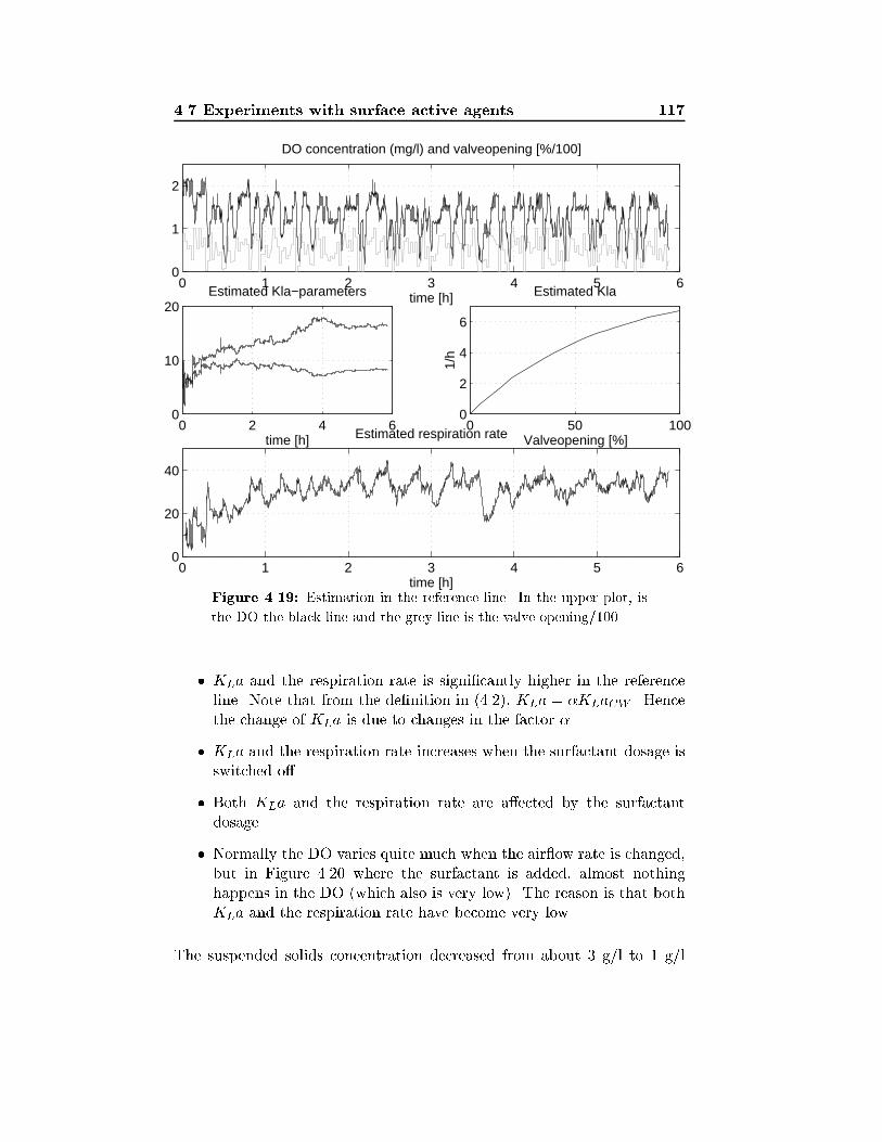
4.7 Experiments with surface active agents 117
0 1 2 3 4 5 60
1
2
time [h]
DO concentration (mg/l) and valveopening [%/100]
0 2 4 60
10
20Estimated Kla−parameters
time [h]0 50 100
0
2
4
6
Estimated Kla
Valveopening [%]1/
h
0 1 2 3 4 5 60
20
40
Estimated respiration rate
time [h]Figure 4.19: Estimation in the reference line. In the upper plot, is
the DO the black line and the grey line is the valve opening/100.
� KLa and the respiration rate is signi�cantly higher in the referenceline. Note that from the de�nition in (4.2), KLa = �KLaCW . Hencethe change of KLa is due to changes in the factor �.
� KLa and the respiration rate increases when the surfactant dosage isswitched o�.
� Both KLa and the respiration rate are a�ected by the surfactantdosage.
� Normally the DO varies quite much when the air ow rate is changed,but in Figure 4.20 where the surfactant is added, almost nothinghappens in the DO (which also is very low). The reason is that bothKLa and the respiration rate have become very low.
The suspended solids concentration decreased from about 3 g/l to 1 g/l
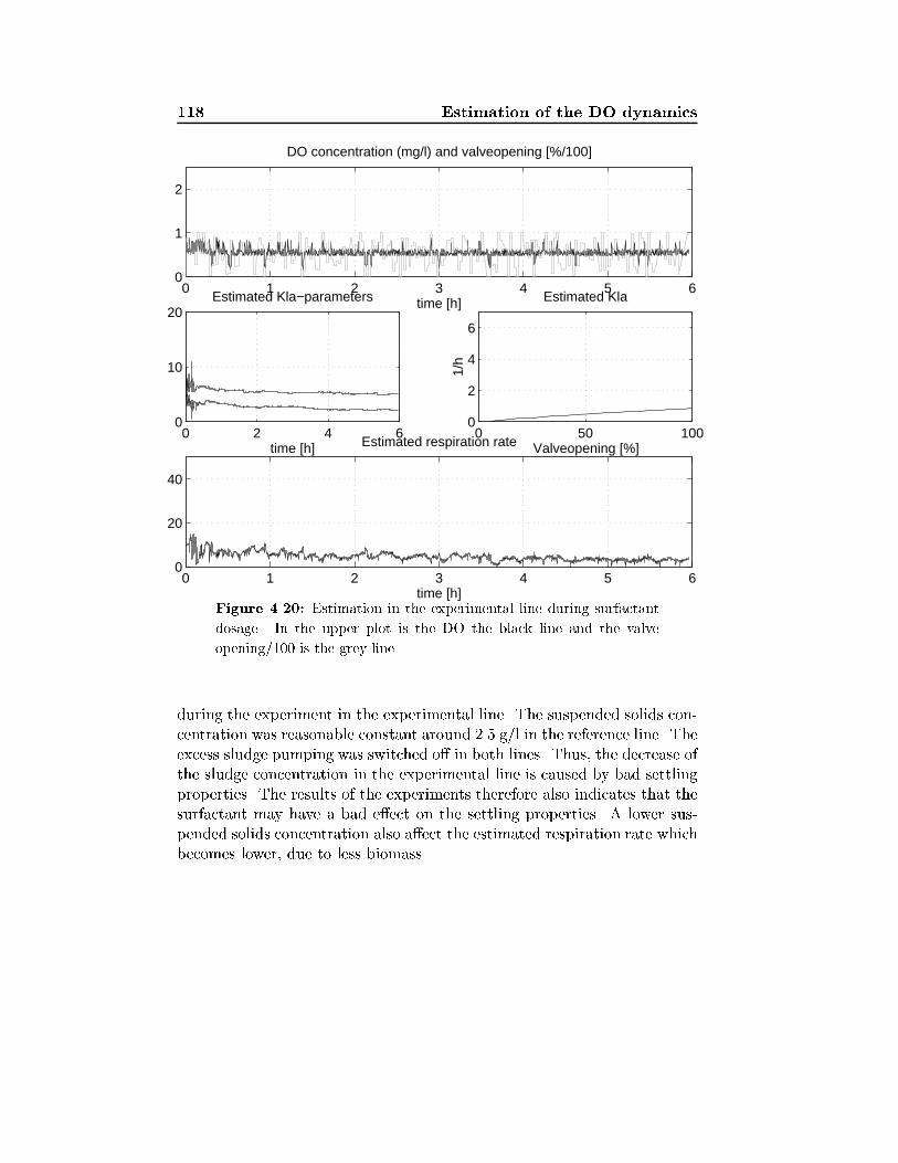
118 Estimation of the DO dynamics
0 1 2 3 4 5 60
1
2
time [h]
DO concentration (mg/l) and valveopening [%/100]
0 2 4 60
10
20Estimated Kla−parameters
time [h]0 50 100
0
2
4
6
Estimated Kla
Valveopening [%]1/
h
0 1 2 3 4 5 60
20
40
Estimated respiration rate
time [h]Figure 4.20: Estimation in the experimental line during surfactant
dosage. In the upper plot is the DO the black line and the valve
opening/100 is the grey line.
during the experiment in the experimental line. The suspended solids con-centration was reasonable constant around 2.5 g/l in the reference line. Theexcess sludge pumping was switched o� in both lines. Thus, the decrease ofthe sludge concentration in the experimental line is caused by bad settlingproperties. The results of the experiments therefore also indicates that thesurfactant may have a bad e�ect on the settling properties. A lower sus-pended solids concentration also a�ect the estimated respiration rate whichbecomes lower, due to less biomass.
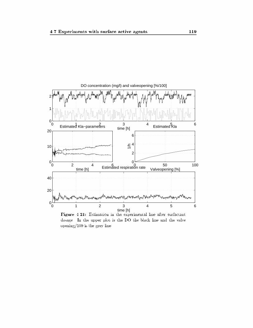
4.7 Experiments with surface active agents 119
0 1 2 3 4 5 60
1
2
time [h]
DO concentration (mg/l) and valveopening [%/100]
0 2 4 60
10
20Estimated Kla−parameters
time [h]0 50 100
0
2
4
6
Estimated Kla
Valveopening [%]
1/h
0 1 2 3 4 5 60
20
40
Estimated respiration rate
time [h]Figure 4.21: Estimation in the experimental line after surfactant
dosage. In the upper plot is the DO the black line and the valve
opening/100 is the grey line.
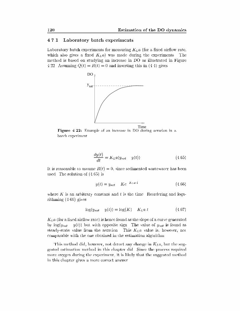
120 Estimation of the DO dynamics
4.7.1 Laboratory batch experiments
Laboratory batch experiments for measuring KLa (for a �xed air ow rate,which also gives a �xed KLa) was made during the experiments. Themethod is based on studying an increase in DO as illustrated in Figure4.22. Assuming Q(t) = R(t) = 0 and inserting this in (4.4) gives
saty
DO
TimeFigure 4.22: Example of an increase in DO during aeration in a
batch experiment.
dy(t)
dt= KLa(ysat � y(t)) (4.65)
It is reasonable to assume R(t) = 0, since sedimented wastewater has beenused. The solution of (4.65) is
y(t) = ysat �Ke�KLa t (4.66)
where K is an arbitrary constant and t is the time. Reordering and loga-rithming (4.66) gives
log(ysat � y(t)) = log(K)�KLa t (4.67)
KLa (for a �xed air ow rate) is hence found as the slope of a curve generatedby log(ysat � y(t)) but with opposite sign. The value of ysat is found assteady-state value from the aeration. This KLa value is, however, notcomparable with the one obtained in the estimation algorithm.
This method did, however, not detect any change in KLa, but the sug-gested estimation method in this chapter did. Since the process requiredmore oxygen during the experiment, it is likely that the suggested methodin this chapter gives a more correct answer.
4.8 Conclusions 121
4.8 Conclusions
Identi�cation algorithms for estimating the time-varying respiration rateand the nonlinear KLa function have been presented. The estimation isbased on measurements of the dissolved oxygen concentration and the air- ow rate. Two di�erent models of the nonlinear KLa function have beensuggested: an exponential model and a cubic spline model. Three mod-els for modeling the respiration rate have also been considered: a randomwalk model, a �ltered random walk model, and an integrated random walkmodel. The exponential model and a cubic spline model were approxi-mately equally good. The �ltered random walk model was the best one ofthe di�erent respiration rate models.
In order to track the time varying respiration rate and the nonlinearKLa function, a Kalman �lter was used. To illustrate the estimation pro-cedure simulation studies have been performed with good results. Theresults from the simulations were also con�rmed on real data from a pilotactivated sludge plant, where the estimated respiration rate was comparedwith batch laboratory measurements. Also, a nonlinear model of the oxy-gen transfer function was achieved.
When the DO sensor has dynamics it should not be neglected. By �l-tering the output from the DO sensor, the in uence of the sensor dynamicscan be reduced. The �ltering procedure may also be useful in other appli-cations where there is need for compensating the sensor dynamics, e.g. inrespirometers.
An experiment with surface active agents was performed and the sug-gested estimation method was applied to detect changes in KLa and therespiration rate. Signi�cant changes were detected in both KLa and therespiration rate which decreased to almost zero. An interesting observationis that when the DO is a�ected by surfactants, the DO is almost constant.The DO will not become lower due to the respiration rate is almost zero,and the DO will not increase by increased air ow rate due to KLa is almostzero.

122 Estimation of the DO dynamics
Chapter 5
Control of the dissolved
oxygen concentration
The dissolved oxygen concentration (DO) in the aerobic part of an acti-vated sludge process should be su�ciently high to supply enough oxygento the microorganisms in the sludge, so organic matter is degraded andammonium is converted to nitrate. On the other hand, an excessively highDO, which requires a high air ow rate, leads to a high energy consumptionand may also deteriorate the sludge quality. A high DO in the internallyrecirculated water also makes the denitri�cation less e�cient, see Olssonand Jeppson (1994). Hence, both for economical and process reasons, it isof interest to control the DO. Several control strategies for the DO havebeen suggested in the past. Flanagan et al. (1977) presented a linear PIcontroller with feedforward from the respiration rate and the ow rate. InWells (1979) di�erent control strategies for the activated sludge processwere applied, among others DO control. A dead-beat controller, based ona recursively estimated model with a linear KLa was designed in Ko et al.(1982). Holmberg et al. (1989) and Bocken et al. (1989) also base their de-sign on a recursively estimated model with a linear KLa, but the excitationof the process was improved by invoking a relay which increases the exci-tation. Pole placement was then used to design the controller. Rundqwist(1986) designed a self-tuning controller, and Carlsson et al. (1994a) haveapplied auto-tuning.
One problem with controlling the DO is that the process dynamicsare nonlinear. This means that high control performance for all operatingconditions may be hard to achieve with a linear controller. The objective ofthe work presented here is a design method which gives a high performance
124 Control of the DO
controller for all operating conditions. The key idea is to explicitly take thenonlinear characteristics of the oxygen transfer function KLa into accountin the control design. The design method consists of two separate parts: anestimation part described in Chapter 4 and a controller design part whichis presented here.
The controller design is based on a linearization of the DO process, ob-tained by using the inverse of the estimated KLa(u). Two di�erent controldesign approaches are suggested for the linearized DO process:
� A pole-placement design with a PI controller
� A linear quadratic (LQ) controller which uses feedforward from therespiration rate upstream.
An advantage compared to auto-tuning of PID-regulators, see �Astr�om andH�agglund (1984) or �Astr�om and Wittenmark (1989), is that the suggestednonlinear controller requires only one single tuning (estimation) event,while auto-tuning of a gain scheduling regulator may require several tuningsfor this type of nonlinear process.
An important issue is the choice of set-point for the DO controller. Inpractice the DO set-point often is kept at some �xed level. A DO set-pointcontroller is suggested, where the set-point is selected so that a prespeci-�ed ammonium concentration in the last aerated zone is obtained, see alsoNielsen and Lynggaard (1993). Using the set-point controller in the pilotplant made it not only possible to save energy due to a lower DO set-point, the e�uent nitrate concentration was also reduced signi�cantly. Thenitrate reduction probably depends on that the lower DO levels made den-itri�cation in the aerated zones possible. The naturally existing carbon inthe aerated zones is then in a larger extent used for denitri�cation insteadof being oxidized. Less oxygen is also recirculated when using a low DOset-point, which improves denitri�cation in the anoxic zone. Possible disad-vantages may be that the sludge properties deteriorate due to the low DO,and that nitrous oxide (N2O) can be formed when the DO is low. Theseproblems should, however, be compared to the achieved improvements.
To save energy the air pressure in the aeration system can be con-trolled. A strategy suggested in, for example Rundqwist (1986) and Robin-son (1990) has been evaluated in the pilot plant with positive result.
The outline of the chapter is as follows. The control problem is pre-sented in Section 5.1, where problems using linear control of a nonlinearprocess are discussed. The controller design of a nonlinear PI-controller
5.1 The control problem 125
and a nonlinear LQ-controller with feedforward are is given in Section 5.2.The di�erent control strategies are compared in some simulation studies inSection 5.3. The proposed controllers are compared at the pilot plant inSection 5.4. Section 5.5 presents a controller for controlling the set-pointof the dissolved oxygen. It is based on control of the ammonium concen-tration. A practical experiment with the DO set-point controller has beenmade in the pilot plant. Section 5.6 gives a short review of a common pres-sure controller which minimizes the pressure drop over the throttle valves.Finally, the conclusions are given in Section 5.7.
5.1 The control problem
The gain of the DO process varies with respect to the air ow rate due to thenonlinear KLa function, see Figure 4.2 and Olsson and Piani (1992). TheDO process also has a bilinear term (KLa(u)y), see further (5.1). This maycause problems when using a linear controller. In Figure 5.1 such a problemis illustrated, where a linear PI-controller is tuned for high performanceduring a high air ow rate but used for a low air ow rate. More examplesare given in Section 5.3. A high air ow rate corresponds here to 80% openvalve. When the load to the plant decreases, the process gain (the derivativeof KLa) increases, and an oscillating system is obtained.
If the linear controller instead was tuned for high performance during alow load, a slow closed loop response would be obtained for a high load. Afair step response for all loads is however possible by taking the nonlinearKLa into account. This is utilized in the following sections.
5.2 The nonlinear DO controller
In the past there has been an extensive research in controller design forlinear systems, and many high performance controllers for linear systemsexist. The DO process is, however, not a linear system. From Chapter4, the following discrete-time model of the dissolved oxygen dynamics wasgiven.
y(t+1) = y(t)+h�[Q(t)
V(yin(t)�y(t))+KLa(u(t))(ysat�y(t))�R(t)] (5.1)
The DO dynamics in (5.1) can be linearized by introducing a variable x(t),de�ned as
x(t) = KLa(u(t))(ysat � y(t)) (5.2)
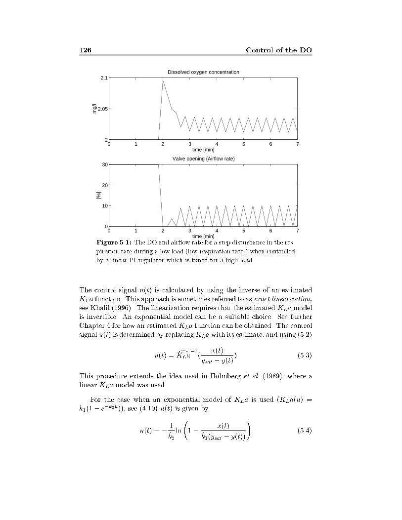
126 Control of the DO
0 1 2 3 4 5 6 72
2.05
2.1Dissolved oxygen concentration
time [min]
mg/
l
0 1 2 3 4 5 6 70
10
20
30Valve opening (Airflow rate)
time [min]
[%]
Figure 5.1: The DO and air ow rate for a step disturbance in the res-
piration rate during a low load (low respiration rate ) when controlled
by a linear PI-regulator which is tuned for a high load.
The control signal u(t) is calculated by using the inverse of an estimatedKLa function. This approach is sometimes referred to as exact linearization,see Khalil (1996). The linearization requires that the estimated KLa modelis invertible. An exponential model can be a suitable choice. See furtherChapter 4 for how an estimated KLa function can be obtained. The controlsignal u(t) is determined by replacingKLa with its estimate, and using (5.2)
u(t) = dKLa�1(
x(t)
ysat � y(t)) (5.3)
This procedure extends the idea used in Holmberg et al. (1989), where alinear KLa model was used.
For the case when an exponential model of KLa is used (KLa(u) =k1(1� e�k2u)), see (4.10) u(t) is given by
u(t) = � 1
k2ln
1� x(t)
k1(ysat � y(t))
!(5.4)

5.2 The nonlinear DO controller 127
-yref �����+
{
-e Controller -x dKLa�1( xysat�y
) -u Process -y
6 6
Figure 5.2: The basic idea with the nonlinear controller.
A block diagram of the linearized process is shown in Figure 5.2.
If the derivative of the estimated KLa is di�erent from the derivative ofthe trueKLa function, the gain of the process model (the derivative ofKLa)will also be di�erent. This may deteriorate the controller performance. Ifthe estimated KLa is smaller than the true, the controller gain will belarger than expected. A too large controller gain may result in a noiseand modeling error sensitive controller. If the estimated KLa becomeslarger than the true KLa the resulting controller will instead be slowerthan expected.
Inserting (5.3) in the process model (5.1) and assuming a correctlyestimated KLa gives the linearized process model
(q � 1 +Q
Vh�)y(t) = h�x(t) + h�
Q
Vyin(t)� h�R(t) (5.5)
Note that the ow (Q) usually is time-varying. When using (5.5) for con-troller design the controller parameters will then also be time-varying.
Remark: In the above discussions we have neglected the valve character-istics. If the valve characteristic is nonlinear, two approaches are possible.
� Use cascade control, where a local controller controls the air ow rate,see Rundqwist (1986) and Robinson (1990). Obviously this approachrequires the air ow rate to be measured.
� Use a model to compensate for the nonlinear valve characteristics.This can easily be incorporated in the KLa model, see further Section4.6.1.
5.2.1 Pole-placement with a PI-controller
Pole-placement will here be used to choose suitable parameters of a PI-regulator. The controller design is performed in two steps. First the closed
128 Control of the DO
loop transfer function is derived, then the controller parameters are deter-mined from a user speci�ed pole-placement, e.g. a double pole.
The transfer function for a continuous-time PI-regulator is
X(s) = K(1 +1
TIs)E(s) (5.6)
where X(s) and E(s) are the Laplace transforms of the controller outputand error signal, K is the proportional gain and TI is the integration time.The error signal is de�ned as
e(t) = yref(t)� y(t) (5.7)
Sampling the PI controller (5.6) with an Euler (backward di�erence) ap-proximation gives
x(t) = K(1 +qh
TI(q � 1))e(t) (5.8)
where h is the sampling period. By combing the transfer function from x(t)to y(t) in (5.5) with the controller (5.8), the closed loop transfer functionfrom yref(t) to y(t) is found to be
HCL(z) =Kh�((1 + h
TI)z � 1)
z2 + z(h�(QV+K + Kh
TI)� 2) + 1� h�(Q
V+K)
(5.9)
To calculate suitable parameter values for K and TI , the closed looppoles are selected to be a double pole in z = p. Complex conjugated poleswould of course also be possible, but will not be considered. Comparingthe poles of (5.9) with the desired pole location
(z � p)2 = z2 � 2zp+ p2 (5.10)
gives two equations, where K and TI are found to be
K =1� p2
h�� Q
V(5.11)
TI =h
1K(2�2p
h�� Q
V)� 1
(5.12)
This method is an easy way of tuning a PI-controller. The user has only tochoose one parameter, the pole location p. The pole location approximatelytrades o� control energy and speed. A double pole close to 1 gives a slowcontroller which is less sensitive to noise and modeling errors, while a polelocation close to the origin gives a fast closed loop system that, however, issensitive system to noise and modeling errors.
5.2 The nonlinear DO controller 129
Remark 1: To calculate the controller parameters K and TI , the param-eter h� is needed, see (4.7). Since it involves KLa(u), which is not known,this might be di�cult. Reasonable choices are to approximate KLa(u) in hwith a �xed value of KLa(u), for example KLa(umax)=2, or to iterate twiceto �nd a reasonable u(t) which determines KLa(u).
Remark 2: Feedforward from yin(t) may be used in combination witha PI-regulator. The feedforward can be derived from (B.23), where thePI-controller has to be expressed in the form of R(q�1) and S(q�1) poly-nomials. An alternative is to use a static feedforward compensator.
Remark 3: The zeros can not be controlled with this structure of thePI controller. Zeros slower than the poles may cause overshoot in the stepresponse despite real valued poles. Unstable zeros cause a non-minimumphase system, where the step response �rst may go in the wrong direction.The zeros can be moved by scaling the reference signal.
Remark 4: The PI controller (5.8) can be implemented in di�erentialform, i.e.
�x(t) = K(�e(t) +h
TIe(t)) (5.13)
x(t) = x(t� 1) +�x(t) (5.14)
which makes it easy to constrain the control signal when it has reached itslimit.
5.2.2 Linear quadratic (LQ) control with feedforward
An LQ controller with feedforward can be applied to the linearized DOprocess (5.5). The controller design is started by rewriting the linearizedDO process model (5.5) into q�1 notation
(1 + q�1(Q
Vh� � 1))y(t) = q�1h�x(t) + q�1h�
Q
Vyin(t)� q�1h�R(t) (5.15)
Assume that the respiration rate and the DO of the input ow can bemodeled as random walks, i.e.
yin(t) =1
�v1(t) R(t) =
1
�v2(t) (5.16)
Adding a term C(q�1) 1�e(t) to describe unmodelled disturbances, the model(5.15) can be written as
A(q�1)y(t) = q�kB(q�1)x(t) + q�d1D1(q�1)
1
�v1(t)
+ q�d2D2(q�1)
1
�v2(t) + C(q�1)
1
�e(t) (5.17)
130 Control of the DO
where the noise sequences v1(t), v2(t) and e(t) are all zero mean white noise,and the polynomials and parameters in are given by
A(q�1) = 1 + q�1(QVh� � 1) D1(q
�1) = h�QV
B(q�1) = h� D2(q�1) = h�
C(q�1) = 1 + cq�1 k = 1 d1 = 1 d2 = 1
The C(q�1) polynomial can be considered as a user parameter and is chosenso that 1=C becomes low-pass, as suggested in Section 3.6.2. This choicemakes the controller less noise sensitive since the high frequency gain isreduced.
The LQ-controller to be used has the following structure
R(q�1)�u(t) = T (q�1)yref (t)�S(q�1)y(t)� Q1(q�1)
P1(q�1)yin(t)� Q2(q
�1)
P2(q�1)R(t)
(5.18)The derivation of the controller polynomials in (5.18) are identical to thecalculations in Section 3.6.3 with b2 = 0. The T (q�1) polynomial is givenby (3.61) in Section 3.7.6.
This controller uses feedforward from both in uent DO and in uentrespiration rate. If all aerated zones are controlled, the in uent DO to azone can then be expected to have small variations. Not much can then begained by using feedforward from in uent water.
The respiration rate can either be measured by a respirometer or es-timated by the algorithm outlined in Chapter 4. Note that it is possibleto �x KLa and only estimate the respiration rate by setting all elementsin the covariance matrix to zero, except for the ones corresponding to therespiration rate. It is then not necessary to use a high excitation in theair ow rate to estimate the respiration rate.
Remark: For the DO process, it is possible to calculate the PI-controllerparameters K and TI from the pole location in �, see (B.12). The PI-controller will, however, not be identical to the LQ-controller, since thePI-controller moves the closed loop zeros, which the LQ-controller doesnot.
5.3 Simulations
In Section 5.1 a simulation example was given where the nonlinearKLa wasnot taken into account in the controller design. This resulted in oscillativecontrol. Some additional examples are given here, where the advantage of
5.3 Simulations 131
nonlinear control is illustrated. An example where feedforward from therespiration rate is applied, is also shown.
5.3.1 Simulation setup
In the simulations in this section the following setup has been used, whichto some extent corresponds to the �rst aerated zone in the pilot plant atKungs�angsverket, see Section 2.1.
The true system has been simulated by (5.1), i.e.
y(t+1) = y(t)+h�[Q(t)
V(yin(t)�y(t))+KLa(u(t))(ysat�y(t))�R(t)] (5.19)
where
� The ow through the zone, Q = 1000 l/h
� The volume of zone, V = 630 l
� The saturated DO, ysat = 10 mg/l
� The in uent DO, yin(t) = 0 mg/l
� The oxygen transfer function, KLa(u) = 15(1 � e�15u(t)1000 ) h�1
� Two cases for variations of the respiration rate R(t) are considered,a low load case and a high load case. In the low load case there is astep from 40 to 5 mg O2/l/h, and in the high load case a step from60 to 85 mg O2/l/h.
� h�(t) = 1A(t) (e
A(t)h � 1), A(t) = �(KLa(u(t)) +Q(t)V
)
� The sampling period, h = 1=360 h
� The KLa used for generating the data and the KLa used in the non-linear controller design are identical.
To get a fair comparison between the linear and nonlinear controller, bothcontrollers should be tuned for equal performance at a given operatingpoint. This can be achieved by adjusting the gain of the controllers appro-priately.
For the linear PI-controller, the controller gain is constant at all op-erating points. This gain is denoted by K lin
PI . The gain of the nonlinear
132 Control of the DO
PI-controller can be considered to consist of two parts. A linear part fromthe PI-controller, denoted Knonlin
PI and the gain from the inverse of the es-timated KLa function. The latter gain is denoted by Knonlin
inv . At a givenoperating point (u0), it is determined by
Knonlininv =
1dKLa(u)
du(ysat � y(t))
ju=u0 (5.20)
The linear and the nonlinear controller becomes equal at a given operatingpoint if
K linPI = Knonlin
inv KnonlinPI (5.21)
This relation will be used in the comparisons.
Remark: The simulations here correspond to values of the pilot plant atKungs�angsverket, where the air ow rate cannot be measured. The air owrate u(t) is instead replaced by the valve opening in the simulations.
5.3.2 Examples
The following simulation examples are given here:
� Fast control of the DO, corresponding to pole placement in 0.5.
� Slower control of the DO, corresponding to pole placement in 0.9.
� LQ control with and without feedforward.
All examples are simulated both for a step change at low load where therespiration rate decreases from 40 to 5 mg O2/l/h, and at a high load wherethe respiration rate increases from 60 to 85 mg O2/l/h.
The parameters of the nonlinear PI-controller are determined by (5.11)and (5.12), and the gain of the linear controller is given by (5.21).
The fast control case is shown in Figure 5.3. The �gure illustratesthat a linear controller which works well for low loads becomes quite slowduring high loads. If the linear controller instead is tuned for a high loadit becomes oscillative for a low load. The nonlinear controller on the otherhand keeps the system well damped at all loads. The reason is that thenonlinear controller change its gain to compensate for the gain changes inthe system.
In the next example, a case is illustrated where the controllers are tunedto be slower than in Figure 5.3. What can be seen in Figure 5.4 is that
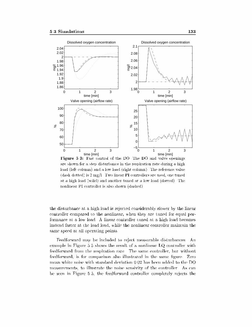
5.3 Simulations 133
0 1 2 3
50
60
70
80
90
100
time [min]
%
Valve opening (airflow rate)
0 1 2 31.861.881.9
1.921.941.961.98
22.022.04
time [min]
mg/
l
Dissolved oxygen concentration
0 1 2 31.98
2
2.02
2.04
2.06
2.08
2.1
time [min]
mg/
l
Dissolved oxygen concentration
0 1 2 3−5
0
5
10
15
20
25
time [min]
%
Valve opening (airflow rate)
Figure 5.3: Fast control of the DO. The DO and valve openings
are shown for a step disturbance in the respiration rate during a high
load (left column) and a low load (right column). The reference value
(dash-dotted) is 2 mg/l. Two linear PI controllers are used, one tuned
at a high load (solid) and another tuned at a low load (dotted). The
nonlinear PI-controller is also shown (dashed).
the disturbance at a high load is rejected considerably slower by the linearcontroller compared to the nonlinear, when they are tuned for equal per-formance at a low load. A linear controller tuned at a high load becomesinstead faster at the load load, while the nonlinear controller maintain thesame speed at all operating points.
Feedforward may be included to reject measurable disturbances. Anexample in Figure 5.5 shows the result of a nonlinear LQ controller withfeedforward from the respiration rate. The same controller, but withoutfeedforward, is for comparison also illustrated in the same �gure. Zeromean white noise with standard deviation 0.02 has been added to the DOmeasurements, to illustrate the noise sensivity of the controller. As canbe seen in Figure 5.5, the feedforward controller completely rejects the
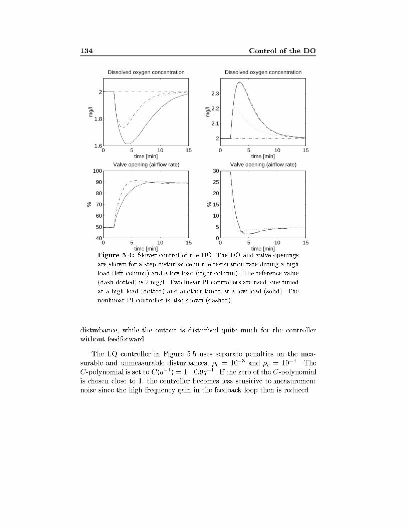
134 Control of the DO
0 5 10 151.6
1.8
2
time [min]
mg/
l
Dissolved oxygen concentration
0 5 10 1540
50
60
70
80
90
100
time [min]
%
Valve opening (airflow rate)
0 5 10 15
2
2.1
2.2
2.3
time [min]
mg/
l
Dissolved oxygen concentration
0 5 10 150
5
10
15
20
25
30
time [min]
%
Valve opening (airflow rate)
Figure 5.4: Slower control of the DO. The DO and valve openings
are shown for a step disturbance in the respiration rate during a high
load (left column) and a low load (right column). The reference value
(dash-dotted) is 2 mg/l. Two linear PI controllers are used, one tuned
at a high load (dotted) and another tuned at a low load (solid). The
nonlinear PI-controller is also shown (dashed).
disturbance, while the output is disturbed quite much for the controllerwithout feedforward.
The LQ controller in Figure 5.5 uses separate penalties on the mea-surable and unmeasurable disturbances, �e = 10�3 and �v = 10�4. TheC-polynomial is set to C(q�1) = 1�0:9q�1. If the zero of the C-polynomialis chosen close to 1, the controller becomes less sensitive to measurementnoise since the high frequency gain in the feedback loop then is reduced.
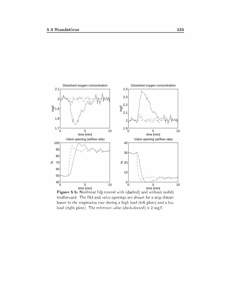
5.3 Simulations 135
0 5 1040
50
60
70
80
90
100
time [min]
%
Valve opening (airflow rate)
0 5 100
10
20
30
40
time [min]
%
Valve opening (airflow rate)
0 5 101.9
2
2.1
2.2
2.3
2.4
time [min]
mg/
l
Dissolved oxygen concentration
0 5 101.7
1.8
1.9
2
2.1
time [min]
mg/
l
Dissolved oxygen concentration
Figure 5.5: Nonlinear LQ control with (dashed) and without (solid)
feedforward. The DO and valve openings are shown for a step distur-
bance in the respiration rate during a high load (left plots) and a low
load (right plots). The reference value (dash-dotted) is 2 mg/l.
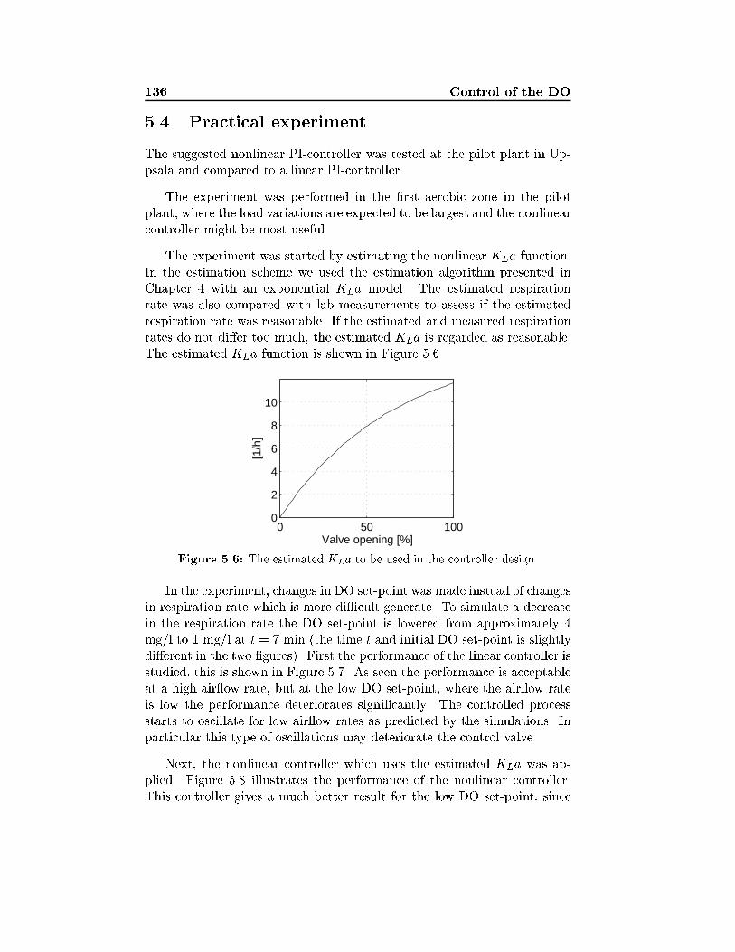
136 Control of the DO
5.4 Practical experiment
The suggested nonlinear PI-controller was tested at the pilot plant in Up-psala and compared to a linear PI-controller.
The experiment was performed in the �rst aerobic zone in the pilotplant, where the load variations are expected to be largest and the nonlinearcontroller might be most useful.
The experiment was started by estimating the nonlinear KLa function.In the estimation scheme we used the estimation algorithm presented inChapter 4 with an exponential KLa model. The estimated respirationrate was also compared with lab measurements to assess if the estimatedrespiration rate was reasonable. If the estimated and measured respirationrates do not di�er too much, the estimated KLa is regarded as reasonable.The estimated KLa function is shown in Figure 5.6.
0 50 1000
2
4
6
8
10
Valve opening [%]
[1/h
]
Figure 5.6: The estimated KLa to be used in the controller design.
In the experiment, changes in DO set-point was made instead of changesin respiration rate which is more di�cult generate. To simulate a decreasein the respiration rate the DO set-point is lowered from approximately 4mg/l to 1 mg/l at t = 7 min (the time t and initial DO set-point is slightlydi�erent in the two �gures). First the performance of the linear controller isstudied, this is shown in Figure 5.7. As seen the performance is acceptableat a high air ow rate, but at the low DO set-point, where the air ow rateis low the performance deteriorates signi�cantly. The controlled processstarts to oscillate for low air ow rates as predicted by the simulations. Inparticular this type of oscillations may deteriorate the control valve.
Next, the nonlinear controller which uses the estimated KLa was ap-plied. Figure 5.8 illustrates the performance of the nonlinear controller.This controller gives a much better result for the low DO set-point, since
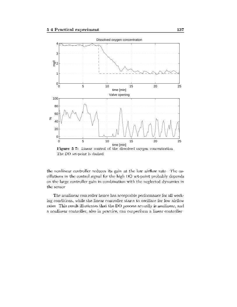
5.4 Practical experiment 137
0 5 10 15 20 250
1
2
3
4
time [min]
mg/
l
Dissolved oxygen concentration
0 5 10 15 20 250
20
40
60
80
100
time [min]
%
Valve opening
Figure 5.7: Linear control of the dissolved oxygen concentration.
The DO set-point is dashed.
the nonlinear controller reduces its gain at the low air ow rate. The os-cillations in the control signal for the high DO set-point probably dependson the large controller gain in combination with the neglected dynamics inthe sensor.
The nonlinear controller hence has acceptable performance for all work-ing conditions, while the linear controller starts to oscillate for low air owrates. This result illustrates that the DO process actually is nonlinear, anda nonlinear controller, also in practice, can outperform a linear controller.
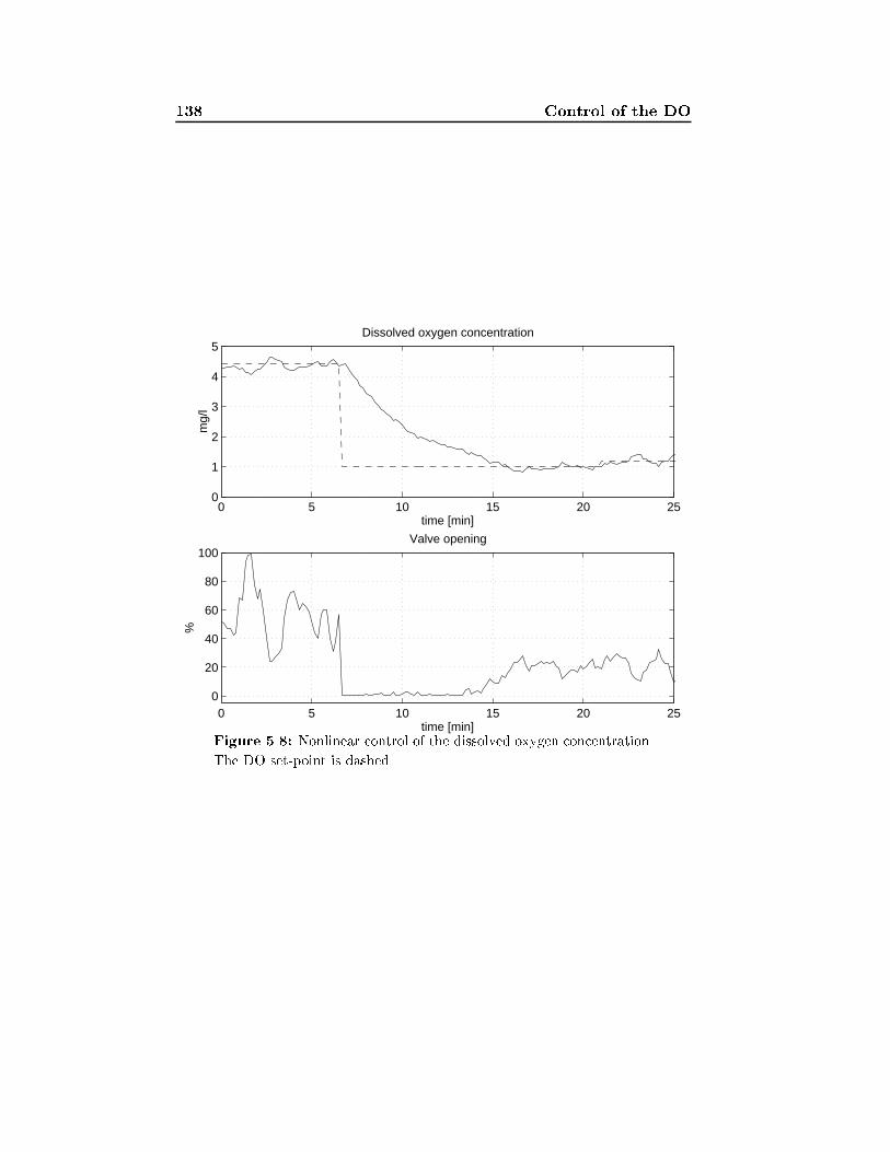
138 Control of the DO
0 5 10 15 20 250
1
2
3
4
5
time [min]
mg/
l
Dissolved oxygen concentration
0 5 10 15 20 250
20
40
60
80
100
time [min]
%
Valve opening
Figure 5.8: Nonlinear control of the dissolved oxygen concentration.
The DO set-point is dashed.

5.5 Control of the dissolved oxygen set-point 139
5.5 Control of the dissolved oxygen set-point
In the aerobic part of an activated sludge process, ammonium is convertedto nitrate by nitri�cation, see also Section 1.3. The nitri�cation processrequires oxygen, which is obtained by blowing air into the tank. Normallya constant DO, controlled by varying the air ow rate guarantees that suf-�cient oxygen is supplied to the process. An alternative to a constant DOset-point is to use a time-varying DO set-point, which is determined bythe ammonium concentration in the last aerobic zone, see also e.g. Nielsenand Lynggaard (1993), and Sorensen et al. (1994) for control of the DOset-point in a Bio-denitroTM process.
The DO set-point control gives or may give the following advantages,depending on the existing plant performance:
� Better control of e�uent ammonium.
� Lower average DO set-point which saves energy (due to a lower airconsumption).
� Lower nitrate concentration in the e�uent, because of improved den-itri�cation due to a lower DO.
� Lower dosage of external carbon (if it is added).
Possible disadvantages may be that the sludge properties deteriorate dueto the low DO, and that nitrous oxide (N2O) can be formed when theDO is low. These problems should, however, be compared to the achievedimprovements. Another variant of DO set-point control may reduce theseproblems. When there are several aerated zones, which often is the case,spatial DO control is possible. The idea is to switch on or o� aeration inthe �rst or last zone(s) when the DO set-point becomes too high or toolow. This latter strategy avoids that the DO set-point becomes too low,and it is probably better than using the same DO set-point in all aeratedzones. This strategy has, however, not been evaluated.
The basic idea is to control the DO set-point from on-line measure-ments of the ammonium concentration, this is illustrated in Figure 5.9.This structure is referred to as cascade control, where the inner DO loopis much faster than outer the ammonium loop. The controller tries tomaintain a prespeci�ed ammonium concentration by varying the DO set-point. To avoid the DO set-point becomes too high or too low, it shouldonly be allowed to vary in an interval e.g. 0.5{4 mg O2/l, which is easilyimplemented.
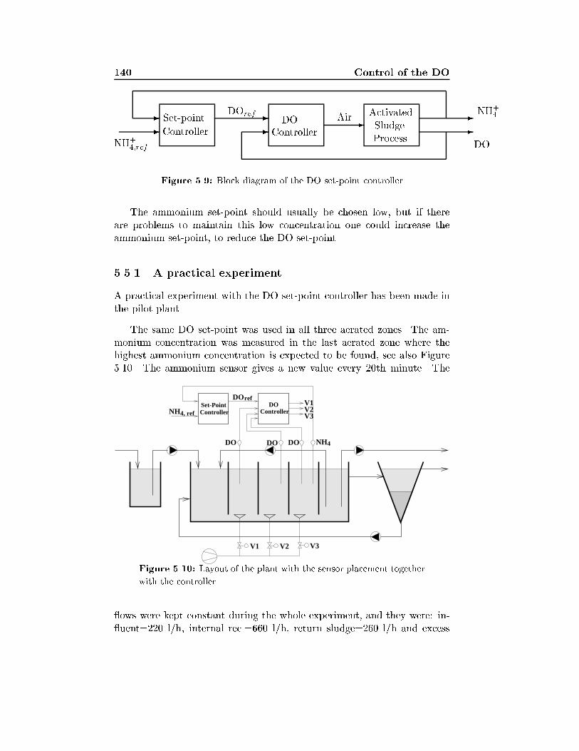
140 Control of the DO
--
----
-Process
Activated
SludgeControllerDOSet-point
Controller
DO
DOref AirNH+
4
NH+4;ref
Figure 5.9: Block diagram of the DO set-point controller
The ammonium set-point should usually be chosen low, but if thereare problems to maintain this low concentration one could increase theammonium set-point, to reduce the DO set-point.
5.5.1 A practical experiment
A practical experiment with the DO set-point controller has been made inthe pilot plant.
The same DO set-point was used in all three aerated zones. The am-monium concentration was measured in the last aerated zone where thehighest ammonium concentration is expected to be found, see also Figure5.10. The ammonium sensor gives a new value every 20th minute. The
DO DODO NH4
4, ref
DOrefV1
V3V2Controller
Set-PointController
DONH
V1 V2 V3
Figure 5.10: Layout of the plant with the sensor placement together
with the controller.
ows were kept constant during the whole experiment, and they were: in- uent=220 l/h, internal rec.=660 l/h, return sludge=260 l/h and excess
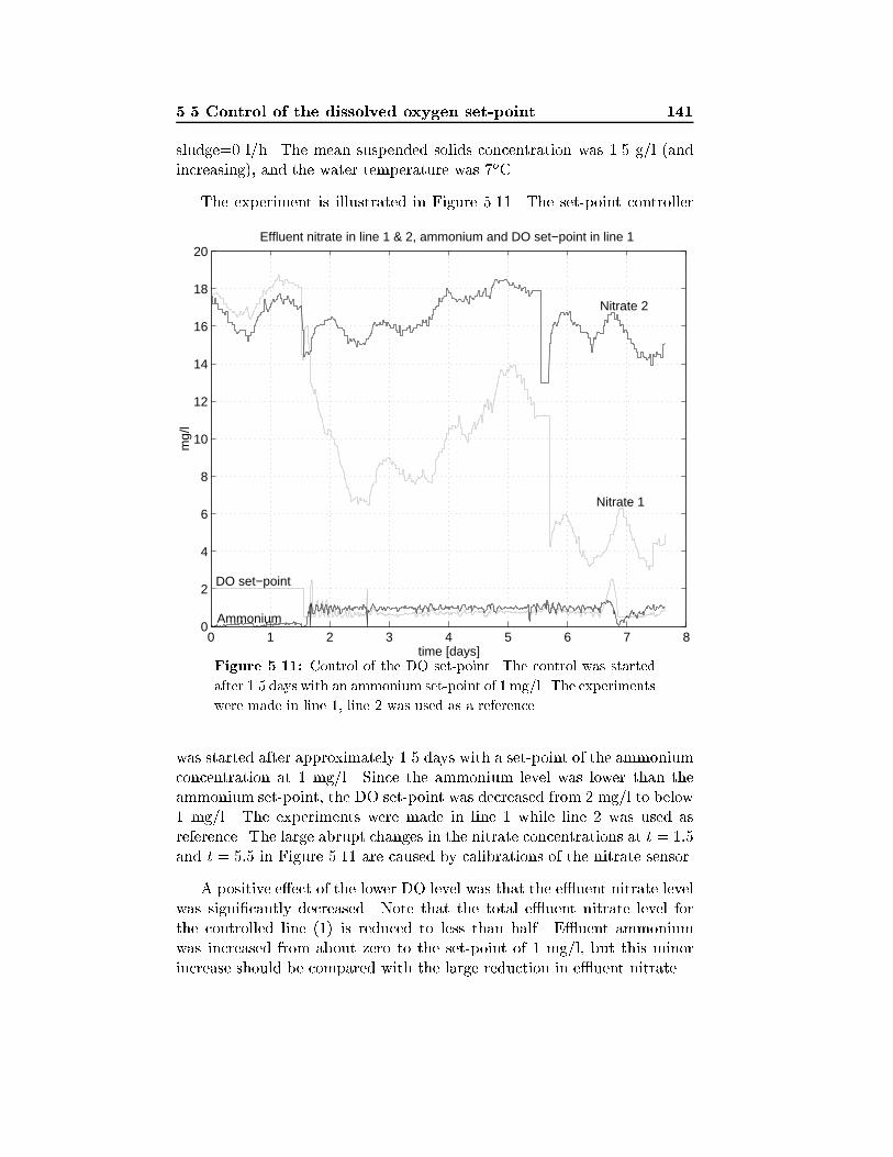
5.5 Control of the dissolved oxygen set-point 141
sludge=0 l/h. The mean suspended solids concentration was 1.5 g/l (andincreasing), and the water temperature was 7oC.
The experiment is illustrated in Figure 5.11. The set-point controller
0 1 2 3 4 5 6 7 80
2
4
6
8
10
12
14
16
18
20Effluent nitrate in line 1 & 2, ammonium and DO set−point in line 1
mg/
l
time [days]
DO set−point
Ammonium
Nitrate 1
Nitrate 2
Figure 5.11: Control of the DO set-point. The control was started
after 1.5 days with an ammonium set-point of 1 mg/l. The experiments
were made in line 1, line 2 was used as a reference.
was started after approximately 1.5 days with a set-point of the ammoniumconcentration at 1 mg/l. Since the ammonium level was lower than theammonium set-point, the DO set-point was decreased from 2 mg/l to below1 mg/l. The experiments were made in line 1 while line 2 was used asreference. The large abrupt changes in the nitrate concentrations at t = 1:5and t = 5:5 in Figure 5.11 are caused by calibrations of the nitrate sensor.
A positive e�ect of the lower DO level was that the e�uent nitrate levelwas signi�cantly decreased. Note that the total e�uent nitrate level forthe controlled line (1) is reduced to less than half. E�uent ammoniumwas increased from about zero to the set-point of 1 mg/l, but this minorincrease should be compared with the large reduction in e�uent nitrate.
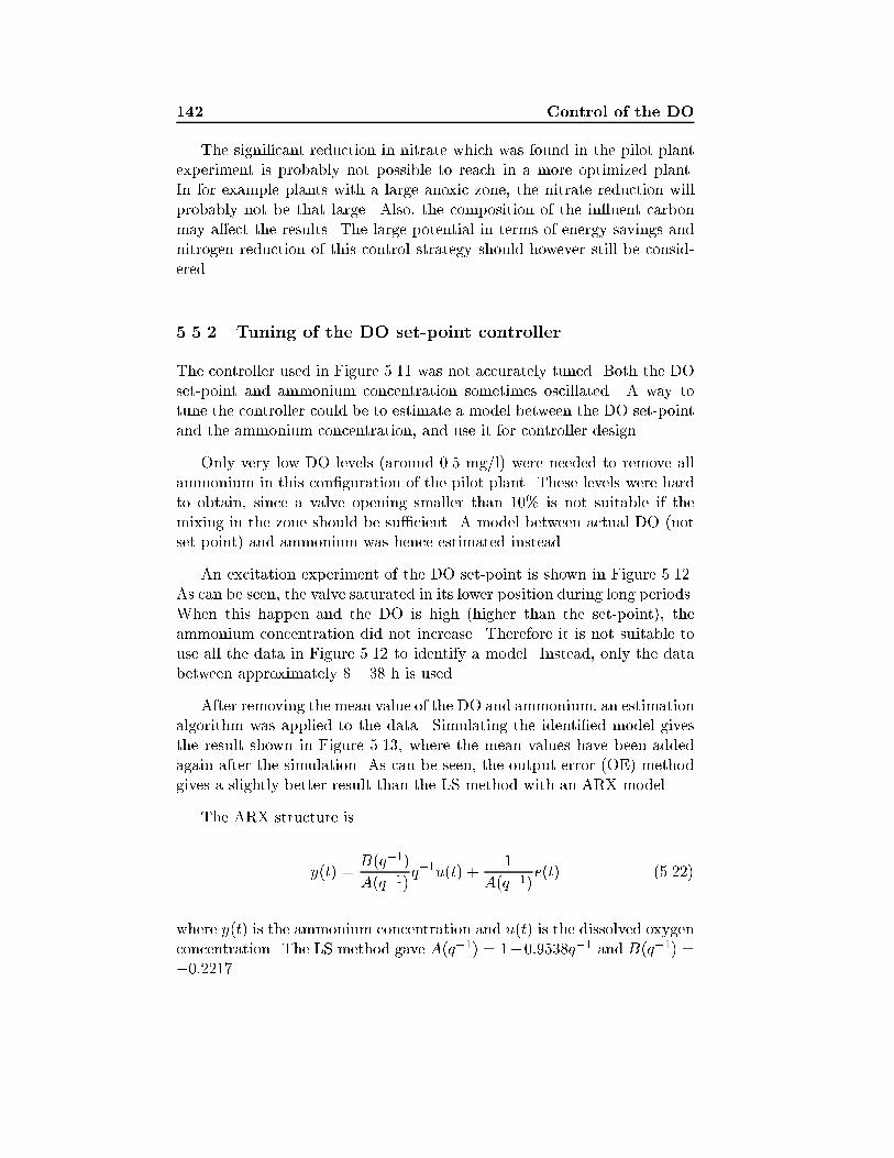
142 Control of the DO
The signi�cant reduction in nitrate which was found in the pilot plantexperiment is probably not possible to reach in a more optimized plant.In for example plants with a large anoxic zone, the nitrate reduction willprobably not be that large. Also, the composition of the in uent carbonmay a�ect the results. The large potential in terms of energy savings andnitrogen reduction of this control strategy should however still be consid-ered.
5.5.2 Tuning of the DO set-point controller
The controller used in Figure 5.11 was not accurately tuned. Both the DOset-point and ammonium concentration sometimes oscillated. A way totune the controller could be to estimate a model between the DO set-pointand the ammonium concentration, and use it for controller design.
Only very low DO levels (around 0.5 mg/l) were needed to remove allammonium in this con�guration of the pilot plant. These levels were hardto obtain, since a valve opening smaller than 10% is not suitable if themixing in the zone should be su�cient. A model between actual DO (notset-point) and ammonium was hence estimated instead.
An excitation experiment of the DO set-point is shown in Figure 5.12.As can be seen, the valve saturated in its lower position during long periods.When this happen and the DO is high (higher than the set-point), theammonium concentration did not increase. Therefore it is not suitable touse all the data in Figure 5.12 to identify a model. Instead, only the databetween approximately 8 { 38 h is used.
After removing the mean value of the DO and ammonium, an estimationalgorithm was applied to the data. Simulating the identi�ed model givesthe result shown in Figure 5.13, where the mean values have been addedagain after the simulation. As can be seen, the output error (OE) methodgives a slightly better result than the LS method with an ARX model.
The ARX structure is
y(t) =B(q�1)
A(q�1)q�1u(t) +
1
A(q�1)e(t) (5.22)
where y(t) is the ammonium concentration and u(t) is the dissolved oxygenconcentration. The LS method gave A(q�1) = 1�0:9538q�1 and B(q�1) =�0:2217.

5.5 Control of the dissolved oxygen set-point 143
0 10 20 30 40 50 60 70 800
0.5
1
1.5DO, DO set−point and valve opening/100
time [h]
0 10 20 30 40 50 60 70 800
1
2Ammonium concentration
mg/
l
time [h]Figure 5.12: Excitation of the DO set-point in the pilot plant, for
generating data to estimate the dynamics between DO set-point and
ammonium concentration. In the upper plot are DO (solid) DO set-
point (dotted) and valve opening/100 (dashed) shown. In the lower
plot, the ammonium concentration is shown.
The output error structure is
y(t) =B(q�1)
A(q�1)q�1u(t) + e(t) (5.23)
Applying the OE method gave A(q�1) = 1 � 0:9675q�1 and B(q�1) =�0:2115.
Some advantages with the OE method are given in S�oderstr�om (1996).They are:
� The estimates may be consistent even if the noise is colored.
� The number of parameters could be chosen low, because the noise isnot modeled.
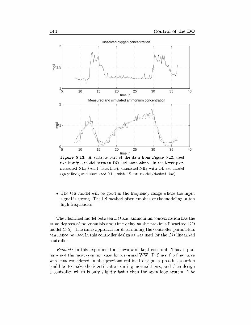
144 Control of the DO
5 10 15 20 25 30 35 400
1
2Measured and simulated ammonium concentration
time [h]
mg/
l
5 10 15 20 25 30 35 401
1.5
2Dissolved oxygen concentration
time [h]
mg/
l
Figure 5.13: A suitable part of the data from Figure 5.12, used
to identify a model between DO and ammonium. In the lower plot,
measured NH4 (solid black line), simulated NH4 with OE-est. model
(grey line), and simulated NH4 with LS-est. model (dashed line).
� The OE model will be good in the frequency range where the inputsignal is strong. The LS method often emphasize the modeling in toohigh frequencies.
The identi�ed model between DO and ammonium concentration has thesame degrees of polynomials and time delay as the previous linearized DOmodel (5.5). The same approach for determining the controller parameterscan hence be used in this controller design as was used for the DO linearizedcontroller.
Remark: In this experiment all ows were kept constant. That is per-haps not the most common case for a normal WWTP. Since the ow rateswere not considered in the previous outlined design, a possible solutioncould be to make the identi�cation during `normal ows, and then designa controller which is only slightly faster than the open loop system. The
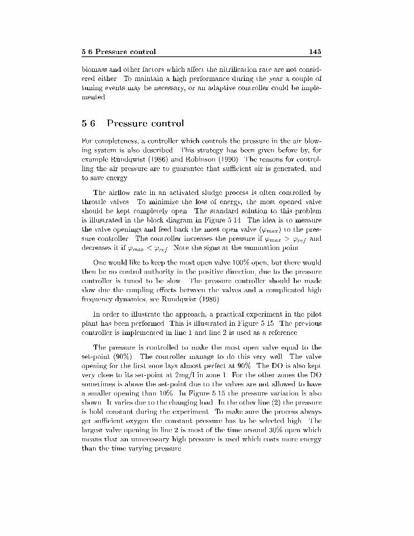
5.6 Pressure control 145
biomass and other factors which a�ect the nitri�cation rate are not consid-ered either. To maintain a high performance during the year a couple oftuning events may be necessary, or an adaptive controller could be imple-mented.
5.6 Pressure control
For completeness, a controller which controls the pressure in the air blow-ing system is also described. This strategy has been given before by, forexample Rundqwist (1986) and Robinson (1990). The reasons for control-ling the air pressure are to guarantee that su�cient air is generated, andto save energy.
The air ow rate in an activated sludge process is often controlled bythrottle valves. To minimize the loss of energy, the most opened valveshould be kept completely open. The standard solution to this problemis illustrated in the block diagram in Figure 5.14. The idea is to measurethe valve openings and feed back the most open valve ('max) to the pres-sure controller. The controller increases the pressure if 'max > 'ref anddecreases it if 'max < 'ref . Note the signs at the summation point.
One would like to keep the most open valve 100% open, but there wouldthen be no control authority in the positive direction, due to the pressurecontroller is tuned to be slow. The pressure controller should be madeslow due the coupling e�ects between the valves and a complicated highfrequency dynamics, see Rundqwist (1986).
In order to illustrate the approach, a practical experiment in the pilotplant has been performed. This is illustrated in Figure 5.15. The previouscontroller is implemented in line 1 and line 2 is used as a reference.
The pressure is controlled to make the most open valve equal to theset-point (90%). The controller manage to do this very well. The valveopening for the �rst zone lays almost perfect at 90%. The DO is also keptvery close to its set-point at 2mg/l in zone 1. For the other zones the DOsometimes is above the set-point due to the valves are not allowed to havea smaller opening than 10%. In Figure 5.15 the pressure variation is alsoshown. It varies due to the changing load. In the other line (2) the pressureis hold constant during the experiment. To make sure the process alwaysget su�cient oxygen the constant pressure has to be selected high. Thelargest valve opening in line 2 is most of the time around 30% open whichmeans that an unnecessary high pressure is used which costs more energythan the time varying pressure.
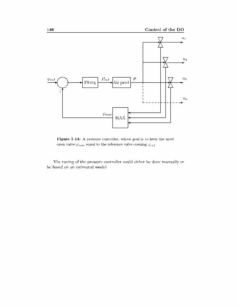
146 Control of the DO
����
PI-reg Air prod.- - - AAA���
AAA ���-
- -
-
--
-
MAX���
��� AAA
6
'ref Pref P
u1
u2
u3
un
�
+
'max
Figure 5.14: A pressure controller, whose goal is to keep the most
open valve 'max equal to the reference valve opening 'ref .
The tuning of the pressure controller could either be done manually orbe based on an estimated model.
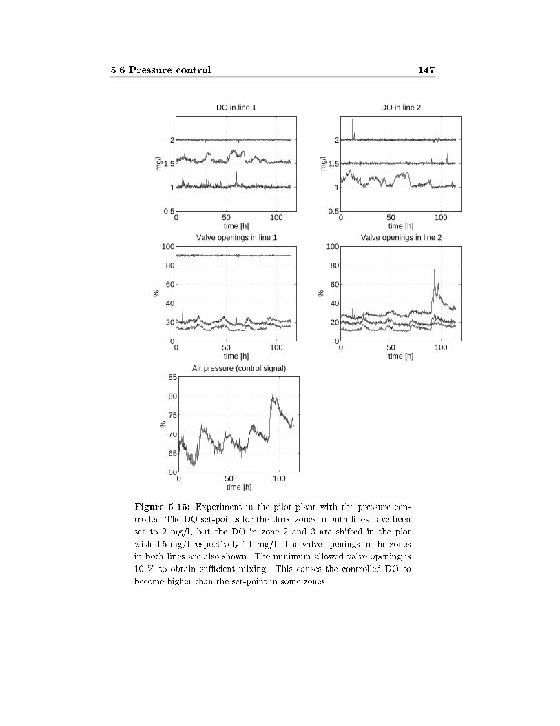
5.6 Pressure control 147
0 50 1000.5
1
1.5
2
DO in line 1
time [h]
mg/
l
0 50 1000.5
1
1.5
2
DO in line 2
time [h]
mg/
l
0 50 1000
20
40
60
80
100Valve openings in line 1
time [h]
%
0 50 1000
20
40
60
80
100Valve openings in line 2
%
time [h]
0 50 10060
65
70
75
80
85Air pressure (control signal)
time [h]
%
Figure 5.15: Experiment in the pilot plant with the pressure con-
troller. The DO set-points for the three zones in both lines have been
set to 2 mg/l, but the DO in zone 2 and 3 are shifted in the plot
with 0.5 mg/l respectively 1.0 mg/l. The valve openings in the zones
in both lines are also shown. The minimum allowed valve opening is
10 % to obtain su�cient mixing. This causes the controlled DO to
become higher than the set-point in some zones.
148 Control of the DO
5.7 Conclusions
The control of the DO in an activated sludge process is an important prob-lem both for economical and process reasons. The basic idea has been toexplicitly take the nonlinear oxygen transfer function KLa into account inthe control design. The oxygen transfer function was found from an estima-tion experiment where a Kalman �lter was used. Two design approacheswere applied on the linearized process: pole-placement with a PI-regulatorand linear quadratic control with feedforward.
In a simulation study, the performance of the controllers were illus-trated. It was shown that the nonlinear DO controller outperforms a stan-dard linear PI controller. The nonlinear controller has also been tested in apilot plant. The tests con�rmed the positive results from the simulations.
A set-point controller for the DO process was presented. The basicidea was to control the DO set-point so that the ammonium concentrationin the last aerobic zone was kept low. An experiment in the pilot plantshowed that, by using this controller not only energy could be saved due toa lower DO set-point, but also the e�uent nitrate concentration becomessigni�cantly lower. How the set-point controller could be tuned was alsodiscussed.
Finally an experiment with a pressure controller in the pilot plant wasmade. It illustrated that it was possible to control the air pressure so thatthe most open valve was almost completely open.
Chapter 6
Multivariable modeling and
control
The activated sludge process is a quite complex process where many statesand nonlinear relations are involved. The process is multivariable, i.e. ithas several inputs and outputs. This means among other things that oneinput a�ects several outputs. For example, a change in the air ow ratea�ect both the ammonium and nitrate concentrations. Another problemis that the activated sludge process is nonlinear, for example the dynamicsdepends on actual ow rates and concentrations.
In this chapter, a linear time-invariant multivariable model is estimatedaround an operating point. The model uses the external carbon ow rate,the internal recirculation rate, and the DO set-point as inputs (the DOset-point can be used as input instead of the air ow rate when cascadecontrol is applied). Ammonium and nitrate in the last aerated zone areused as outputs. The model also includes in uent ow rate, in uent am-monium and in uent carbon (substrate) as measurable disturbances. Theestimated model is then used for controller design. Two di�erent integrat-ing LQ controllers are designed which uses feedforward from the measurabledisturbances.
The main advantage of such a controller is that it takes the interac-tions in the process model into account and an optimal (in an LQ sense)trade-o� between the di�erent inputs and outputs can be utilized. In thepast, mostly SISO (single input single output) control strategies have beensuggested for control of the nitrate and ammonium concentration. Forexample, Londong (1992) controlled the nitrate level by varying the inter-
150 Multivariable modeling and control
nal recirculation rate and Lindberg and Carlsson (1996a) by varying thedosage of an external carbon source. The ammonium concentration can becontrolled by the DO. This has been demonstrated in e.g. Lindberg andCarlsson (1996d) and Sorensen et al. (1994). Few examples of multivari-able control applied to wastewater treatment is found in the literature, andthose who are found have not controlled the ammonium and nitrate level.For examples, Dochain and Perrier (1993), Bastin and Dochain (1990),and Youssef et al. (1995) have designed multivariable controllers, but onlyvalidated their control strategy on simpli�ed models.
6.1 Modeling
As mentioned previously, the activated sludge process is a complex processwhere many components and nonlinear relations are involved. It is hencea delicate problem to �nd a model which su�ciently well describe thisprocess. One way to �nd such a model is to use physical knowledge of theprocess. Several such models have been suggested, and the most widely usedone is probably the IAWQ model, presented by Henze et al. (1987), see alsoChapter 2. This model contains 13 coupled nonlinear di�erential equationsand around 20 more or less unknown parameters. An activated sludgeprocess also consists of several zones and a settler. The IAWQ model onlydescribes one zone. Several IAWQ models therefore have to be connected toeach other in order to model a bioreactor. Finally a settler model, about ascomplex as the IAWQ model, also has to be included. It is not easy to tunesuch a model or use it for controller design. Another approach to modelingis to use a black-box model, which is linear and time invariant. A systemidenti�cation method can then be applied to estimate its parameters frominput-output data. Such a model is suitable for controller design, whichis the main purpose here. It will also be shown (by simulations) that theidenti�ed black-box model, describes the activated sludge process well, atleast around an operating point. A drawback with this type of model isthat the physical insight of the process is lost. For example, the states arearti�cial and it is not possible to understand how a process variable, whichnot is directly included in the model, a�ects the process. An advantage isthat this model only needs input/output data to be estimated.
Since the activated sludge process is nonlinear we may need di�erentsets of linear models to be able to approximate the process at di�erentoperating points. When the activated sludge process is controlled we tryto stay around an operating point. This reduces the nonlinear e�ects, andit may be su�cient with only one linear model. It will also be shown (by
6.1 Modeling 151
simulations) that the estimated model works well for large changes in bothin uent ows and in uent concentrations. If, however, one linear modelcan not approximate the real process, a couple of models may be used atdi�erent operating points.
Grey-box modeling, where parts of the physical model structure is in-cluded, could be an alternative to black-box modeling. Since the structureis very complex in the connected IAWQ models and the settler model, suchan approach has been abandoned.
6.1.1 What to model?
What to model is an interesting question. Often one knows what to modelsince the inputs and outputs are known, and the model establishes a relationbetween these signals. For an activated sludge process it is, however, notclear what should be considered as an input or an output. This dependsamong other things on the purpose of the model. Where to measure is notobvious either.
The purpose of the modeling is, as mentioned before, to use the derivedmodel for controller design. In an activated sludge process it is desired tokeep the e�uent ammonium concentration and the e�uent nitrate concen-tration at low levels. Our aim will therefore be to control these concentra-tions, and keep them close to the desired set-points.
The activated sludge process contains dynamics with time constantswhich range from seconds (e.g. pressure in air pipes) to weeks (e.g. sludgeretention time). To cover all dynamics in one model is not suitable. Abetter solution is to divide the model into a couple of smaller models whichapproximately have the same time constants. The set-point of a fast processcan then be controlled by a slower process (cascade control). In that waythe fast dynamics may be neglected when considering the slower models.An example is a model of the dissolved oxygen concentration (DO), whereonly the relation between DO and air ow rate is included, the relationbetween valve position and the air ow rate is excluded. Here, the set-pointof the DO is considered as an input instead of e.g. air ow rate.
From e.g. Olsson and Jeppson (1994) we �nd that the following controlhandles: external carbon dosage, internal recirculation rate, and DO set-point a�ect the ammonium and nitrate concentrations, and they also do itin approximately the same time scale (hours). Hence, these three controlvariables will therefore be used as inputs. As outputs we consider ammo-nium and nitrate. To improve the model, in uent ow, in uent carbon
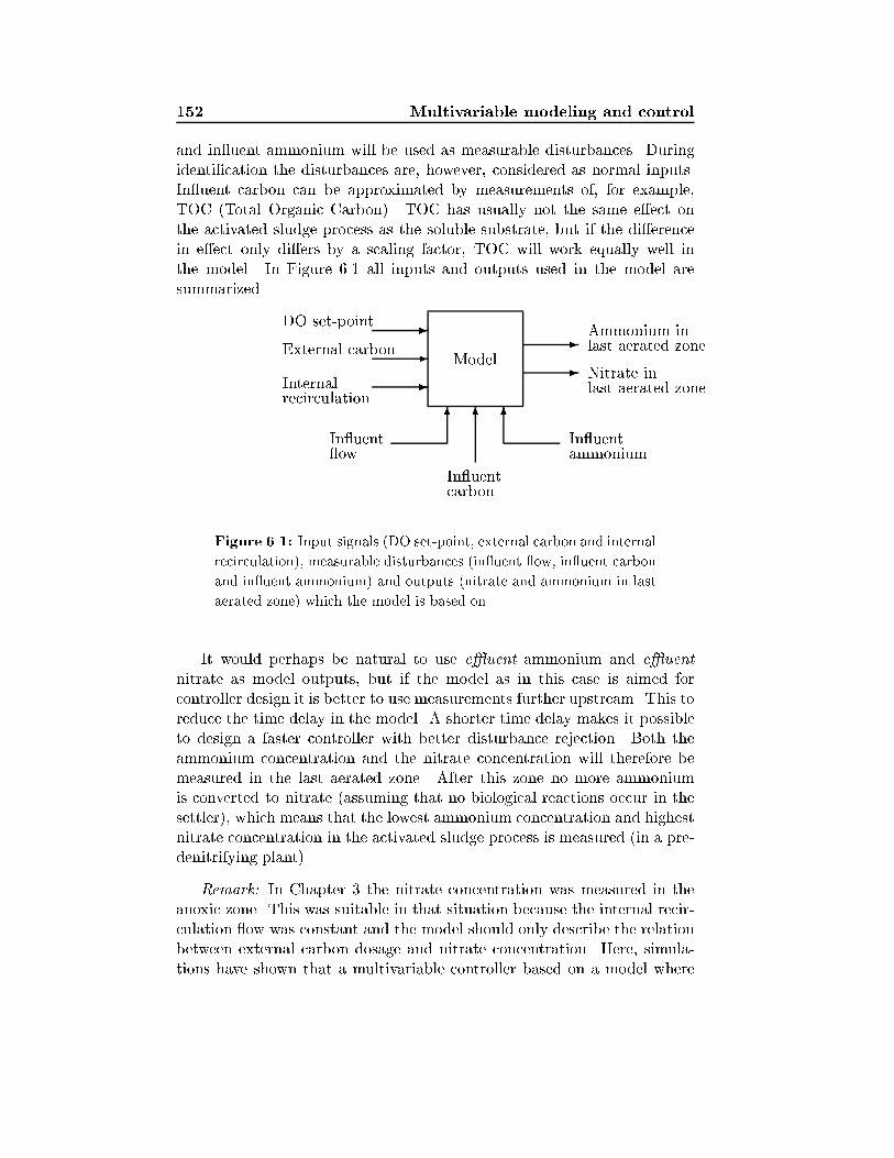
152 Multivariable modeling and control
and in uent ammonium will be used as measurable disturbances. Duringidenti�cation the disturbances are, however, considered as normal inputs.In uent carbon can be approximated by measurements of, for example,TOC (Total Organic Carbon). TOC has usually not the same e�ect onthe activated sludge process as the soluble substrate, but if the di�erencein e�ect only di�ers by a scaling factor, TOC will work equally well inthe model. In Figure 6.1 all inputs and outputs used in the model aresummarized.
Model-
-
-
-
-
66 6
DO set-point
External carbon
Internalrecirculation
In uent ow
In uentcarbon
In uentammonium
Nitrate inlast aerated zone
Ammonium inlast aerated zone
Figure 6.1: Input signals (DO set-point, external carbon and internal
recirculation), measurable disturbances (in uent ow, in uent carbon
and in uent ammonium) and outputs (nitrate and ammonium in last
aerated zone) which the model is based on
It would perhaps be natural to use e�uent ammonium and e�uent
nitrate as model outputs, but if the model as in this case is aimed forcontroller design it is better to use measurements further upstream. This toreduce the time delay in the model. A shorter time delay makes it possibleto design a faster controller with better disturbance rejection. Both theammonium concentration and the nitrate concentration will therefore bemeasured in the last aerated zone. After this zone no more ammoniumis converted to nitrate (assuming that no biological reactions occur in thesettler), which means that the lowest ammonium concentration and highestnitrate concentration in the activated sludge process is measured (in a pre-denitrifying plant).
Remark: In Chapter 3 the nitrate concentration was measured in theanoxic zone. This was suitable in that situation because the internal recir-culation ow was constant and the model should only describe the relationbetween external carbon dosage and nitrate concentration. Here, simula-tions have shown that a multivariable controller based on a model where
6.1 Modeling 153
the nitrate concentration in the anoxic zone is an output will fail. Sucha controller switch o� the internal recirculation, probably due to the factthat the nitri�cation process is badly modeled. By switching o� the inter-nal recirculation, it is easy to maintain a low nitrate concentration in theanoxic zone for a pre-denitrifying activated sludge process, but the e�uentnitrate concentration will be rather high.
6.1.2 Subspace identi�cation
For SISO (Single Input Single Output) systems polynomial models like AR-MAX models are convenient both for identi�cation and controller designpurposes. For MIMO (Multiple Input Multiple Output) systems, poly-nomial models are complex, since they become matrix fraction decompo-sitions. In these models it is not obvious how to choose the polynomialdegrees and the time delays. An alternative to polynomial models, is touse Subspace State Space System Identi�cation (4SID). The advantages arethat the user has relatively few design variables, the methods have robustnumerical properties, and relatively low computational complexity (Viberget al. 1995).
A short introduction to subspace identi�cation
The problem formulation in subspace identi�cation is as follows: Giveninput and output measurements, �nd an appropriate order n and systemmatrices (Van Overschee and De Moor 1996). This is a very general formu-lation and in system identi�cation which could �t to many identi�cationmethods. The solution to the problem in the subspace based techniques is,however, quite di�erent compared to the techniques based on an iterativesearch. The subspace methods uses projections and singular value decom-positions to �nd the model. The following derivation is mostly taken fromViberg (1994) who gives an overview of existing subspace based techniques.
Assume that the true system can be described by
x(t+ 1) = Ax(t) +Bu(t) (6.1)
y(t) = Cx(t) +Du(t) (6.2)

154 Multivariable modeling and control
and de�ne
U =
2666666666664
u(0) u(1) u(2) : : : u(j � 1)u(1) u(2) u(3) : : : u(j)...
......
...u(i� 1) u(i) u(i+ 1) : : : u(i+ j � 2)u(i) u(i+ 1) u(i+ 2) : : : u(i+ j � 1)...
......
...u(2i� 1) u(2i) u(2i+ 1) : : : u(2i+ j � 2)
3777777777775(6.3)
where the number of columns j typically is chosen to j = N�2i+1 so thatall data are used. Matrices for the output Y and the state X are generatedin the same way as for the input U , replace all u with y respectively x.The parameter i is a user parameter, similar to the number of block rowsin some algorithms, e.g. N4SID1.
Introduce the extended observability matrix � and the lower blockToeplitz matrix H
� =
266664CCA...
CA2i�1
377775 H =
266664D 0 : : : 0CB D : : : 0...
.... . .
...CA2i�2B CA2i�3B : : : D
377775 (6.4)
The following matrix equation can then be derived
Y = �X +HU (6.5)
and the orthogonal projection onto the null space of U , introduced as
�?UT = I � UT (UUT )�1U (6.6)
Multiplying (6.5) by �?UT
gives
Y�?UT = �X�?UT (6.7)
since U�?UT
= 0. Now, make a singular value composition of Y�?UT
andpartition it as
Y�?UT = QsSsVTs +QnSnV
Tn (6.8)
where the Q matrices contains the left singular vectors, the S matrices arediagonal matrices with the corresponding singular values, and the V ma-trices contains the right singular vectors. The product of the matrices with
1Numerical algorithms for Subspace State Space System Identi�cation (Van Overscheeand De Moor 1996).
6.1 Modeling 155
the index s contains the signal subspace, and the product of the matriceswith the index n contains the noise subspace. In absence of noise Sn = 0.Data from a real process always contains noise, hence Sn 6= 0. One thenhave to �nd the border between Ss and Sn. A common approach is thento set the border where the singular values drop to small values.
The observability matrix � is then estimated by
� = Qs (6.9)
In fact, � should be chosen so that R(�) = R(Qs). The particular choice(6.9) is simple and corresponds to a speci�c realization dependent choiceof coordinates. The system matrix A is found from � through the relation
�2:n = �1:n�1A (6.10)
where �2:n is � with the �rst block row deleted and �1:n�1 is � with thelast block row deleted. The system of equations (6.10) is over-determinedin the unknown matrix A, and can be solved in several ways. The C matrixis given by the �rst row(s) of �, according to (6.4).
Multiplying (6.5) with QTn yields
QTnY = QT
nHU (6.11)
which gives an over-determined system of equations that can be solved ina least squares sense with respect to B and D. Note that QT
n� = 0 since� = Qs, which is orthogonal to Qn.
The presented algorithm is just one of many variants. There existsmethods which are more e�cient and take care of process and measurementnoise, see e.g. Van Overschee and De Moor (1996).
6.1.3 Application of subspace identi�cation to the activatedsludge process
In Section 6.1.1 it was concluded that a model should be found which mod-els the two outputs, nitrate and ammonium in the last aerated zone, basedon the three inputs DO set-point, external carbon, internal recirculation,and the three measurable disturbances in uent ow, in uent carbon andin uent ammonium.
A discrete-time model is estimated from the input-output data usingsubspace identi�cation:
x(t+ 1) = Fx(t) +Gu(t) +Gdd(t) (6.12)
y(t) = Cx(t) (6.13)

156 Multivariable modeling and control
where y(t) is the outputs, u(t) the inputs, d(t) the measurable disturbances,and x(t) is a state vector. The state vector x(t) is \arti�cial", created bythe subspace algorithm, and it does usually not contain any measurablestates. The other parameters in (6.12) and (6.13), i.e. F , G, Gd, and C arematrices.
The structure of (6.12) is not directly suitable for identi�cation. It canbe rewritten such that the measurable disturbances d(t) are considered asinputs and included in the input vector as
x(t+ 1) = Fx(t) + [ G Gd ]
"u(t)d(t)
#(6.14)
Generation of data
It is very important to excite the input signals in a sensible way to beable to estimate a linear black-box model from input-output data. Theinput signals should have a su�cient excitation in both amplitude andfrequency. The output concentrations should not deviate too much fromnormal operating levels.
The activated sludge process is simulated by the model presented inSection 2.3 with the input signals given in Figure 6.2 and measurabledisturbances in Figure 6.3. The return sludge ow in Figure 6.4 is alsovaried, but not included in the model. The internal recirculation, and re-turn sludge, were generated by low pass �ltering white noise. Values abovethe maximum limit or below the minimum limit have been set to the limitfor each control signal. The gain and bandwidth of the low pass �lters isdi�erent for the di�erent signals, as well as the mean values. The exci-tation of the DO set-point was the most critical signal to generate. Theactivated sludge process is very nonlinear for DO values close to zero. Toavoid that the ammonium concentration, which also depends on the DO,becomes large, a PID controller for the DO set-point is used, as outlinedin Section 5.5. The DO set-point is hence generated by a PID controllerduring the simulation. The PID controller tries to follow a reference signalin the ammonium concentration by varying the DO set-point. The ammo-nium reference signal is excited by PRBS (Pseudo Random Binary Signals).This (usually) gives a control signal with reasonable excitation in both am-plitude and frequency. The reason for that the ammonium concentration inFigure 6.5 does not look like a PRBS is that the PID controller constrainsthe DO set-point between 0.2 { 4 mg/l. The carbon ow rate was gener-ated in a similar way as the DO set-point. The nitrate concentration in theanxoic zone was controlled by the controller outlined in Section 3.4. The
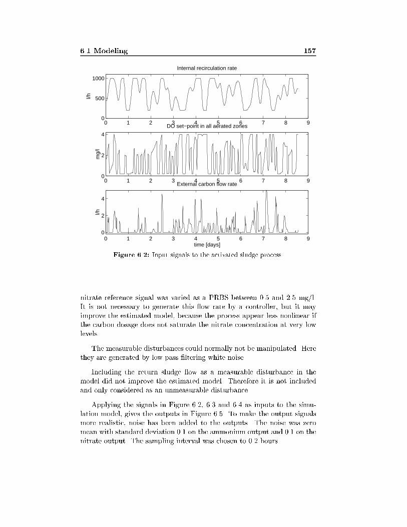
6.1 Modeling 157
0 1 2 3 4 5 6 7 8 90
500
1000
l/h
Internal recirculation rate
0 1 2 3 4 5 6 7 8 90
2
4
mg/
l
DO set−point in all aerated zones
0 1 2 3 4 5 6 7 8 90
2
4
time [days]
l/h
External carbon flow rate
Figure 6.2: Input signals to the activated sludge process.
nitrate reference signal was varied as a PRBS between 0.5 and 2.5 mg/l.It is not necessary to generate this ow rate by a controller, but it mayimprove the estimated model, because the process appear less nonlinear ifthe carbon dosage does not saturate the nitrate concentration at very lowlevels.
The measurable disturbances could normally not be manipulated. Herethey are generated by low pass �ltering white noise.
Including the return sludge ow as a measurable disturbance in themodel did not improve the estimated model. Therefore it is not includedand only considered as an unmeasurable disturbance.
Applying the signals in Figure 6.2, 6.3 and 6.4 as inputs to the simu-lation model, gives the outputs in Figure 6.5. To make the output signalsmore realistic, noise has been added to the outputs. The noise was zeromean with standard deviation 0.1 on the ammonium output and 0.1 on thenitrate output. The sampling interval was chosen to 0.2 hours.
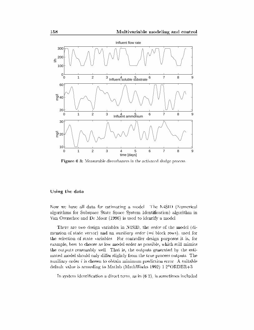
158 Multivariable modeling and control
0 1 2 3 4 5 6 7 8 90
100
200
300
l/h
Influent flow rate
0 1 2 3 4 5 6 7 8 910
20
30
time [days]
mg/
l
Influent ammonium0 1 2 3 4 5 6 7 8 9
20
40
60
mg/
l
Influent soluble substrate
Figure 6.3: Measurable disturbances in the activated sludge process.
Using the data
Now we have all data for estimating a model. The N4SID (Numericalalgorithms for Subspace State Space System Identi�cation) algorithm inVan Overschee and De Moor (1996) is used to identify a model.
There are two design variables in N4SID, the order of the model (di-mension of state vector) and an auxiliary order (=i block rows), used forthe selection of state variables. For controller design purposes it is, forexample, best to choose as low model order as possible, which still mimicsthe outputs reasonably well. That is, the outputs generated by the esti-mated model should only di�er slightly from the true process outputs. Theauxiliary order i is chosen to obtain minimum prediction error. A suitabledefault value is according to Matlab (MathWorks 1992) 1.2*ORDER+3.
In system identi�cation a direct term, as in (6.2), is sometimes included
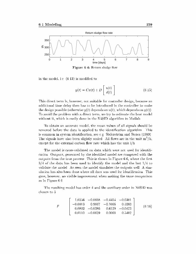
6.1 Modeling 159
0 1 2 3 4 5 6 7 8 9
250
300
350
time [days]
l/h
Return sludge flow rate
Figure 6.4: Return sludge ow.
in the model, i.e. (6.13) is modi�ed to
y(t) = Cx(t) +D
"u(t)d(t)
#(6.15)
This direct term is, however, not suitable for controller design, because anadditional time delay then has to be introduced in the controller to makethe design possible (otherwise y(t) depends on u(t), which depends on y(t)).To avoid the problem with a direct term, we try to estimate the best modelwithout it, which is easily done in the N4SID algorithm in Matlab.
To obtain an accurate model, the mean values of all signals should beremoved before the data is applied to the identi�cation algorithm. Thisis common in system identi�cation, see e.g. S�oderstr�om and Stoica (1989).The signals have also been slightly scaled. All ows are in the unit m3/h,except for the external carbon ow rate which has the unit l/h.
The model is cross-validated on data which were not used for identi�-cation. Outputs, generated by the identi�ed model are compared with theoutputs from the true process. This is shown in Figure 6.6, where the �rst3/4 of the data has been used to identify the model and the last 1/4 tovalidate the model. As seen the model simulates the outputs well. A sim-ulation has also been done where all data was used for identi�cation. Thisgave, however, no visible improvement when making the same comparisonas in Figure 6.6.
The resulting model has order 4 and the auxiliary order in N4SID waschosen to 5.
F =
266641:0356 �0:0668 �0:4454 �0:0301
�0:0013 0:9667 �0:1066 0:52830:0802 �0:0386 0:6120 �0:04730:0110 �0:0629 0:0069 0:5402
37775 (6.16)
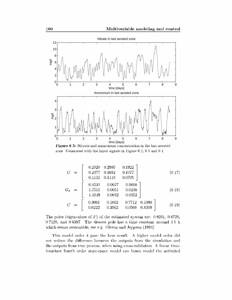
160 Multivariable modeling and control
0 1 2 3 4 5 6 7 8 90
2
4
6
8
10
12
time [days]
mg/
l
Nitrate in last aerated zone
0 1 2 3 4 5 6 7 8 90
1
2
3
4
time [days]
mg/
l
Ammonium in last aerated zone
Figure 6.5: Nitrate and ammonium concentration in the last aerated
zone. Generated with the input signals in Figure 6.2, 6.3 and 6.4.
G =
264 �0:2920 0:2985 �0:1922�0:2377 0:1682 0:1077�0:1155 0:1119 0:0705
375 (6.17)
Gd =
264 �0:4531 �0:0027 �0:0066�1:7515 0:0051 �0:0236�1:4949 0:0032 �0:0352
375 (6.18)
C =
"0:3081 0:1062 0:7712 0:1098
�0:0222 �0:3962 �0:0508 0:8309
#(6.19)
The poles (eigenvalues of F ) of the estimated system are: 0.9291, 0.8728,0.7128, and 0.6397. The slowest pole has a time constant around 4.5 hwhich seems reasonable, see e.g. Olsson and Jeppson (1994).
This model order 4 gave the best result. A higher model order didnot reduce the di�erence between the outputs from the simulation andthe outputs from true process, when using cross-validation. A linear time-invariant fourth order state-space model can hence model the activated
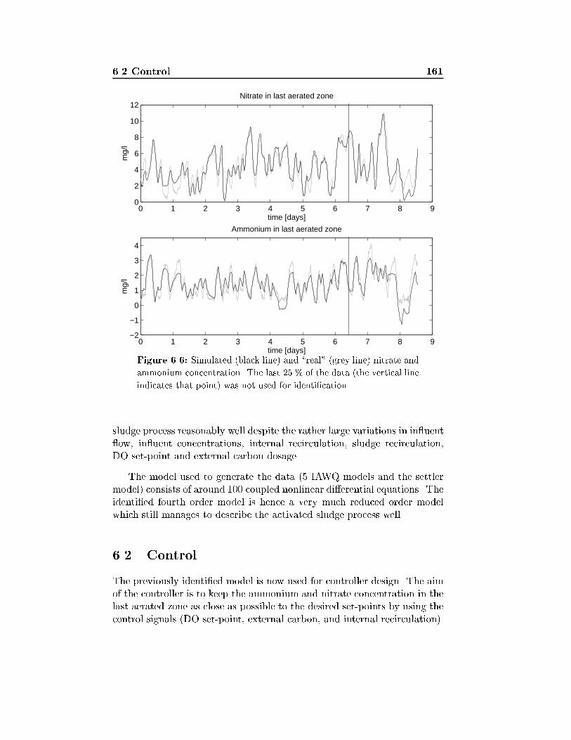
6.2 Control 161
0 1 2 3 4 5 6 7 8 9−2
−1
0
1
2
3
4
time [days]
mg/
l
Ammonium in last aerated zone
0 1 2 3 4 5 6 7 8 90
2
4
6
8
10
12
time [days]
mg/
l
Nitrate in last aerated zone
Figure 6.6: Simulated (black line) and \real" (grey line) nitrate and
ammonium concentration. The last 25 % of the data (the vertical line
indicates that point) was not used for identi�cation.
sludge process reasonably well despite the rather large variations in in uent ow, in uent concentrations, internal recirculation, sludge recirculation,DO set-point and external carbon dosage.
The model used to generate the data (5 IAWQ models and the settlermodel) consists of around 100 coupled nonlinear di�erential equations. Theidenti�ed fourth order model is hence a very much reduced order modelwhich still manages to describe the activated sludge process well.
6.2 Control
The previously identi�ed model is now used for controller design. The aimof the controller is to keep the ammonium and nitrate concentration in thelast aerated zone as close as possible to the desired set-points by using thecontrol signals (DO set-point, external carbon, and internal recirculation).
162 Multivariable modeling and control
Feedforward from in uent ow, in uent carbon and in uent ammoniumis also applied. To make the controller able to remove stationary errors,integration is included.
It should be stressed that the most critical part in the controller designis to obtain a good model. A su�ciently good model may be estimated ifthe input signals are designed with care, like in the previous section.
6.2.1 Controller design
In Section 6.1.3 a state-space model (6.12) of the process was identi�ed
x(t+ 1) = Fx(t) +Gu(t) +Gdd(t) (6.20)
y(t) = Cx(t) (6.21)
The state vector can be augmented with the measurable disturbances d(t)as
"x(t+ 1)d(t+ 1)
#=
"F Gd
0 Fd
# "x(t)d(t)
#+
"G0
#u(t) +
"vx(t)vd(t)
#(6.22)
y(t) = [ C 0 ]
"x(t)d(t)
#+ e(t) (6.23)
where the zeros are matrices of suitable size �lled with zeros. By includingd(t) in the state vector, the feedforward design in the LQ controller willbe convenient, see also Kwakernaak and Sivan (1972). To include d(t) inthe state vector, its dynamic has to be modeled, and therefore the matrixparameter Fd is included. It could e.g. be selected as Fd = 0:99I, whichalmost makes d(t) a random walk process. To make the measurable dis-turbance d(t) not be completely deterministic (which it of course is not),the noise vd(t) has been added. The noises vx(t), vd(t) and e(t) are notused in the controller design, they are only included for completeness. Inan observer design their variances could be used as design variables.
There exists di�erent strategies to design an integrating controller. Twoapproaches will be studied. The �rst one is based on di�erentiating thesystem and deriving an incremental controller, see e.g. Garc��a et al. (1989).This approach is commonly used in Model Predictive Control (MPC). Thesecond approach is to include additional integration states for each output,see e.g. �Astr�om and Wittenmark (1990).
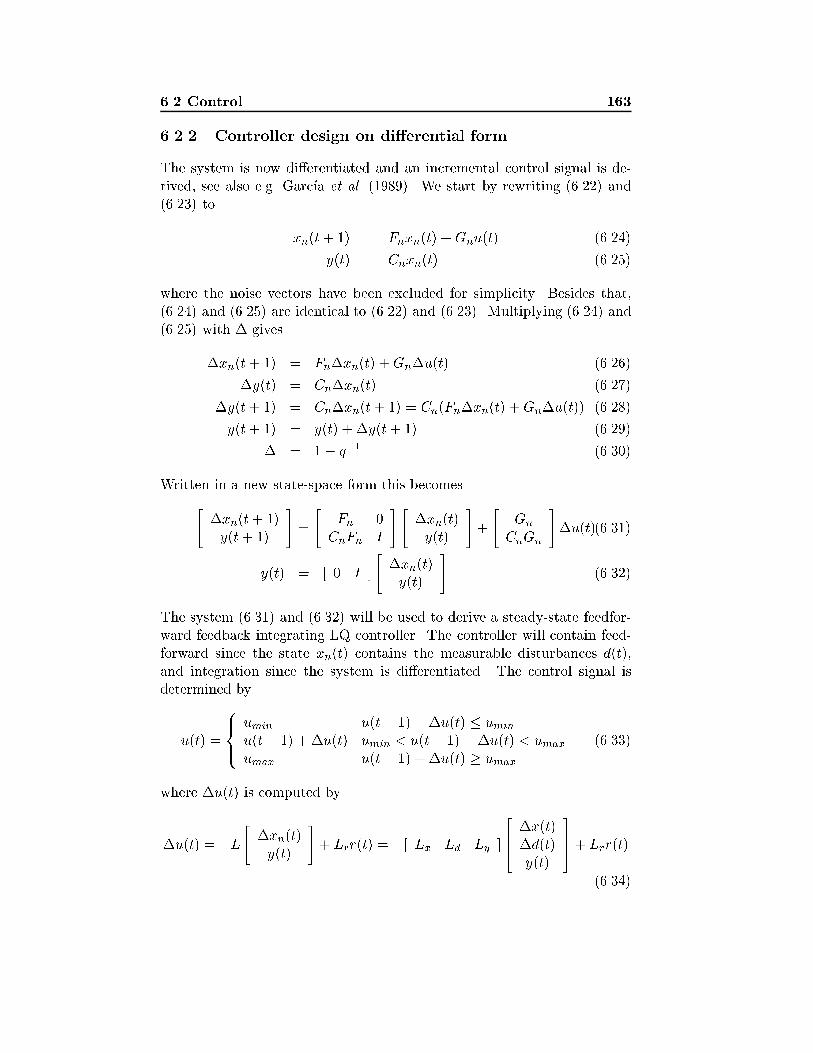
6.2 Control 163
6.2.2 Controller design on di�erential form
The system is now di�erentiated and an incremental control signal is de-rived, see also e.g. Garc��a et al. (1989). We start by rewriting (6.22) and(6.23) to
xn(t+ 1) = Fnxn(t) +Gnu(t) (6.24)
y(t) = Cnxn(t) (6.25)
where the noise vectors have been excluded for simplicity. Besides that,(6.24) and (6.25) are identical to (6.22) and (6.23). Multiplying (6.24) and(6.25) with � gives
�xn(t+ 1) = Fn�xn(t) +Gn�u(t) (6.26)
�y(t) = Cn�xn(t) (6.27)
�y(t+ 1) = Cn�xn(t+ 1) = Cn(Fn�xn(t) +Gn�u(t)) (6.28)
y(t+ 1) = y(t) + �y(t+ 1) (6.29)
� = 1� q�1 (6.30)
Written in a new state-space form this becomes"�xn(t+ 1)y(t+ 1)
#=
"Fn 0CnFn I
# "�xn(t)y(t)
#+
"Gn
CnGn
#�u(t)(6.31)
y(t) = [ 0 I ]
"�xn(t)y(t)
#(6.32)
The system (6.31) and (6.32) will be used to derive a steady-state feedfor-ward feedback integrating LQ controller. The controller will contain feed-forward since the state xn(t) contains the measurable disturbances d(t),and integration since the system is di�erentiated. The control signal isdetermined by
u(t) =
8><>:umin u(t� 1) + �u(t) � uminu(t� 1) + �u(t) umin < u(t� 1) + �u(t) < umaxumax u(t� 1) + �u(t) � umax
(6.33)
where �u(t) is computed by
�u(t) = �L"�xn(t)y(t)
#+ Lrr(t) = �[ Lx Ld Ly ]
264 �x(t)�d(t)y(t)
375+ Lrr(t)
(6.34)
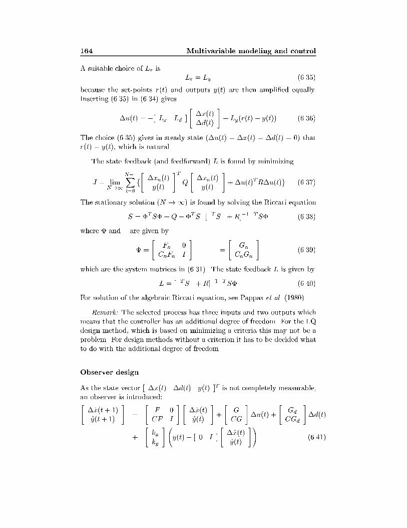
164 Multivariable modeling and control
A suitable choice of Lr isLr = Ly (6.35)
because the set-points r(t) and outputs y(t) are then ampli�ed equally.Inserting (6.35) in (6.34) gives
�u(t) = �[ Lx Ld ]
"�x(t)�d(t)
#+ Ly(r(t)� y(t)) (6.36)
The choice (6.35) gives in steady state (�u(t) = �x(t) = �d(t) = 0) thatr(t) = y(t), which is natural.
The state feedback (and feedforward) L is found by minimizing
J = limN!1
N�1Xt=0
f"�xn(t)y(t)
#TQ
"�xn(t)y(t)
#+�u(t)TR�u(t)g (6.37)
The stationary solution (N !1) is found by solving the Riccati equation
S = �TS�+Q� �TS�[�TS� +R]�1�TS� (6.38)
where � and � are given by
� =
"Fn 0CnFn I
#� =
"Gn
CnGn
#(6.39)
which are the system matrices in (6.31). The state feedback L is given by
L = [�TS� +R]�1�TS� (6.40)
For solution of the algebraic Riccati equation, see Pappas et al. (1980).
Remark: The selected process has three inputs and two outputs whichmeans that the controller has an additional degree of freedom. For the LQdesign method, which is based on minimizing a criteria this may not be aproblem. For design methods without a criterion it has to be decided whatto do with the additional degree of freedom.
Observer design
As the state vector [ �x(t) �d(t) y(t) ]T is not completely measurable,an observer is introduced:"�x(t+ 1)y(t+ 1)
#=
"F 0CF I
# "�x(t)y(t)
#+
"GCG
#�u(t) +
"Gd
CGd
#�d(t)
+
"kxky
# y(t)� [ 0 I ]
"�x(t)y(t)
#!(6.41)
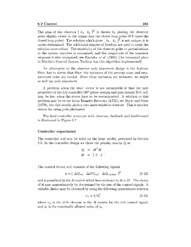
6.2 Control 165
The gain of the observer [ kx ky ]T is chosen by placing the observerpoles slightly closer to the origin than the closed loop poles (0.9 times theclosed loop poles). The solution which gives [ kx ky ]T is not unique, it isunder-determined. The additional degrees of freedom are used to make thesolution more robust. The sensitivity of the observer poles to perturbationsin the system matrices is minimized, and the magnitude of the transientresponse is also minimized, see Kautsky et al. (1985) (the command place
in Matlab's Control System Toolbox has this algorithm implemented).
An alternative to the observer pole placement design is the Kalman�lter, but to derive that �lter, the variances of the process noise and mea-surement noise are needed. Since these variances are unknown, we mightas well use pole placement.
A problem when the state vector is not measurable is that the niceproperties of the LQ controller (60o phase margin and gain margin ]0:5;1[)may be lost when the states have to be reconstructed. A solution to thisproblem may be to use Loop Transfer Recovery (LTR), see Doyle and Stein(1979), but this usually gives a very noise sensitive observer. This is anotherreason for using pole placement.
The �nal controller structure with observer, feedback and feedforwardis illustrated in Figure 6.7.
Controller experiment
The controller will now be tried on the large model, presented in Section2.3. In the controller design we chose the penalty matrix Q as
Q = HTH
H = [ 0 I ]
The control vector u(t) consists of the following signals
u = [ �Qint �DOref �QCarbon ]T (6.42)
and is penalized by the R-matrix which here is chosen to R = 2I. The choiceof R may approximately be determined by the size of the control signals. Asuitable choice may be obtained by using the following approximate relation
rii = 1=~u2i (6.43)
where rii is the ii:th element in the R matrix for the i:th control signal,and ~ui is the maximally allowed value of ui.
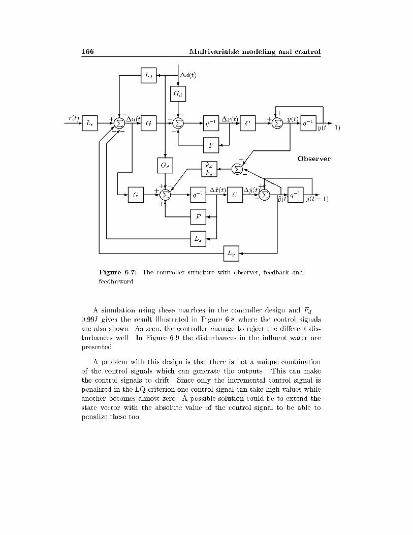
166 Multivariable modeling and control
� ��P � ��P � ��P
� ��P � ��P� ��P
- - -
?
?
�
- - - - - -?
�6
G
Gd
Lr
Ld
q�1
F
C q�1
G
Gd
q�1
F
C q�1
Lx
Ly
kxky
- - - - - -?
�6
?
�
����
����
�
?
����/
�
HHHH
HHY
?
-
..................................................................................................................................
..................................................................................................................................
..
..
..
..
..
..
..
..
..
..
..
..
..
..
..
..
..
..
..
..
..
.
..
..
..
..
..
..
..
..
..
..
..
..
..
..
..
..
..
..
..
..
..
.���/
+�
��
++
+
++
+
�
++ +
+
+
+
r(t) y(t)
y(t� 1)
y(t� 1)
�d(t)
y(t)
�x(t)�u(t)
�x(t) �y(t)
Observer
Figure 6.7: The controller structure with observer, feedback and
feedforward.
A simulation using these matrices in the controller design and Fd =0:99I gives the result illustrated in Figure 6.8 where the control signalsare also shown. As seen, the controller manage to reject the di�erent dis-turbances well. In Figure 6.9 the disturbances in the in uent water arepresented.
A problem with this design is that there is not a unique combinationof the control signals which can generate the outputs. This can makethe control signals to drift. Since only the incremental control signal ispenalized in the LQ criterion one control signal can take high values whileanother becomes almost zero. A possible solution could be to extend thestate vector with the absolute value of the control signal to be able topenalize these too.
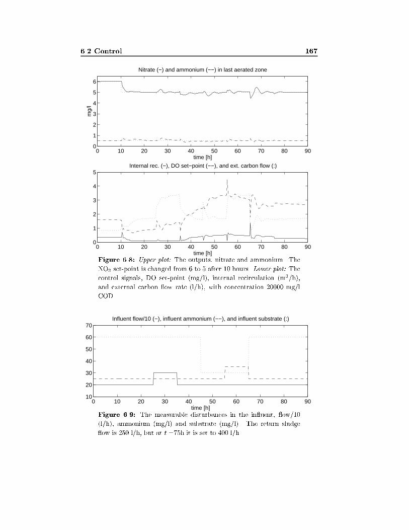
6.2 Control 167
0 10 20 30 40 50 60 70 80 900
1
2
3
4
5
time [h]
Internal rec. (−), DO set−point (−−), and ext. carbon flow (:)
0 10 20 30 40 50 60 70 80 900
1
2
3
4
5
6
time [h]
mg/
l
Nitrate (−) and ammonium (−−) in last aerated zone
Figure 6.8: Upper plot: The outputs, nitrate and ammonium. The
NO3 set-point is changed from 6 to 5 after 10 hours. Lower plot: The
control signals, DO set-point (mg/l), internal recirculation (m3/h),
and external carbon ow rate (l/h), with concentration 20000 mg/l
COD.
0 10 20 30 40 50 60 70 80 9010
20
30
40
50
60
70
time [h]
Influent flow/10 (−), influent ammonium (−−), and influent substrate (:)
Figure 6.9: The measurable disturbances in the in uent, ow/10
(l/h), ammonium (mg/l) and substrate (mg/l). The return sludge
ow is 250 l/h, but at t =75h it is set to 400 l/h.
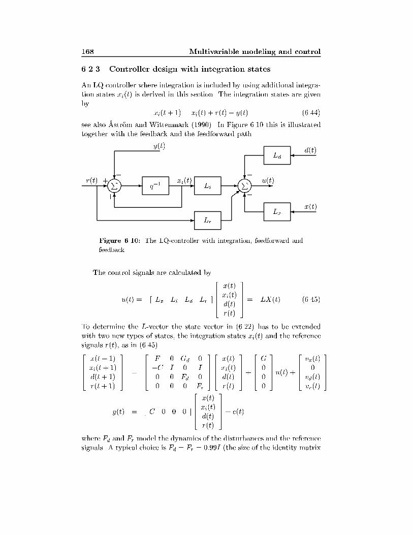
168 Multivariable modeling and control
6.2.3 Controller design with integration states
An LQ controller where integration is included by using additional integra-tion states xi(t) is derived in this section. The integration states are givenby
xi(t+ 1) = xi(t) + r(t)� y(t) (6.44)
see also �Astr�om and Wittenmark (1990). In Figure 6.10 this is illustratedtogether with the feedback and the feedforward path.
����P ����Pq�1 Li
Lr
Lx
Ld
- - - - -?
6
-
��>
�
6
?
�
r(t)
y(t)
x(t)
u(t)
d(t)
xi(t)+�
+
��
�
�
Figure 6.10: The LQ-controller with integration, feedforward and
feedback.
The control signals are calculated by
u(t) = �[ Lx Li Ld Lr ]
26664x(t)xi(t)d(t)r(t)
37775 = �LX(t) (6.45)
To determine the L-vector the state vector in (6.22) has to be extendedwith two new types of states, the integration states xi(t) and the referencesignals r(t), as in (6.45).26664x(t+ 1)xi(t+ 1)d(t+ 1)r(t+ 1)
37775 =
26664F 0 Gd 0�C I 0 I0 0 Fd 00 0 0 Fr
3777526664x(t)xi(t)d(t)r(t)
37775+26664G000
37775u(t) +26664vx(t)0
vd(t)vr(t)
37775
y(t) = [ C 0 0 0 ]
26664x(t)xi(t)d(t)r(t)
37775+ e(t)
where Fd and Fr model the dynamics of the disturbances and the referencesignals. A typical choice is Fd = Fr = 0:99I (the size of the identity matrix
6.2 Control 169
I is, however, di�erent for Fd and Fr). The new system is now used forcalculating the L-vector which is found by minimizing the LQ criterion
J =1Xt=0
X(t)TQX(t) + u(t)TRu(t) (6.46)
The minimum is found by solving the Riccati equation, see (6.38). Notethat � and � are di�erent here than in (6.38).
In (6.46), the Q and R matrices have to be selected. A suitable quantityto penalize with the Q matrix can be
r(t)� y(t) + �xi(t) (6.47)
which means that the control error (r� y) and a scaled part of the integra-tion state xi is penalized. The parameter � is a user parameter. Setting� = 0 leaves out xi which gives a controller without integration. Penalizingonly xi usually gives a controller with bad performance.
This particular penalty choice in (6.47) gives with � = 0:2
Q = HTH
H = [ �C 0:2I 0 I ]
The control vector u(t) which in this case consists of
u = [ Qint DOref QCarbon ]T (6.48)
is penalized in the LQ criterion by the R-matrix, which is chosen to
R =
264 0:5 0 00 0:5 00 0 2
375 (6.49)
Remark: Another idea to select the Q and R matrices could be to letthese matrices in some way represent economical fees for e�uent concen-trations and prices of running pumps, external carbon dosing, etc. TheLQ controller could then be based on the criterion J =
P1t=0[y(t)
TQy(t) +u(t)TRu(t)], where no integration is included. One could then hope thatthe LQ controller should �nd the optimal operating point. This did, how-ever, not work well (the process was drifting around a lot) probably due tothe criterion contains squared signals instead of linear signals.
170 Multivariable modeling and control
Observer design
In this observer design it is only necessary to estimate x(t). In the incremen-tal design, outlined in Section 6.2.2, both �x(t) and y(t) were estimated.Here x(t) is estimated by
x(t+ 1) = F x(t) +Gu(t) +Gdd(t) +K(y(t)� Cx(t)) (6.50)
The gain of the observer K is chosen by placing the observer poles slightlyfaster than closed loop poles (0.9 times the closed loop poles F�GLx). Thesolution is under-determined and the additional degrees of freedom is usedto make the observer more robust to perturbations in the system matrices,similar to the observer design in Section 6.2.2.
Antiwindup
To avoid integrator windup, where the integration states grow when a con-trol signal has saturated, the integration states are not updated if a controlsignal has saturated. Hence
xi(t+ 1) =
(xi(t) + r(t)� y(t) if no control signal has saturatedxi(t) when any control signal has saturated
(6.51)The control signal which saturates can now be limited without achieving anunacceptable performance. Note that the observer has to use the saturatedcontrol signals.
Controller experiment
In Figure 6.11 an application with the controller is illustrated. The distur-bances are the same as in Figure 6.9. It is interesting to study how thecontroller trades o� the di�erent signals. Changing the NO3 reference sig-nal from 6 to 5, at t = 10h, causes the external carbon dosage and internalrecirculation to increase, the DO set-point decrease and the ammonium be-comes temporarily higher. An almost doubled return sludge ow at t=75hdoes hardly not a�ect the control, which is in agreement with the identi�-cation experiment, where it was found that using the return sludge ow asan input did not improve the estimated model.
The previous simulation was noise-free. The same simulation is nowrepeated, but with noise added on the output with standard deviation 0.1on the ammonium sensor and 0.1 on the nitrate sensor. This is illustratedin Figure 6.12. As seen, the control signals becomes a bit noisy. A less
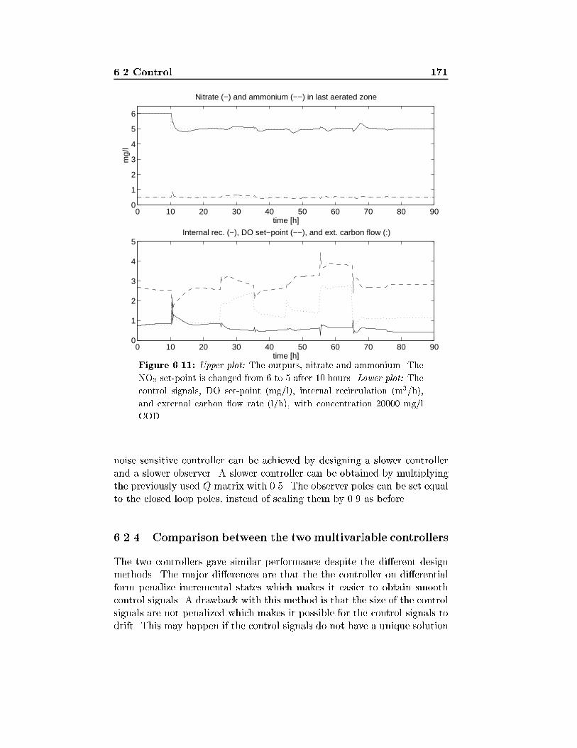
6.2 Control 171
0 10 20 30 40 50 60 70 80 900
1
2
3
4
5
6
time [h]
mg/
l
Nitrate (−) and ammonium (−−) in last aerated zone
0 10 20 30 40 50 60 70 80 900
1
2
3
4
5
time [h]
Internal rec. (−), DO set−point (−−), and ext. carbon flow (:)
Figure 6.11: Upper plot: The outputs, nitrate and ammonium. The
NO3 set-point is changed from 6 to 5 after 10 hours. Lower plot: The
control signals, DO set-point (mg/l), internal recirculation (m3/h),
and external carbon ow rate (l/h), with concentration 20000 mg/l
COD.
noise sensitive controller can be achieved by designing a slower controllerand a slower observer. A slower controller can be obtained by multiplyingthe previously used Q matrix with 0.5. The observer poles can be set equalto the closed loop poles, instead of scaling them by 0.9 as before.
6.2.4 Comparison between the two multivariable controllers
The two controllers gave similar performance despite the di�erent designmethods. The major di�erences are that the the controller on di�erentialform penalize incremental states which makes it easier to obtain smoothcontrol signals. A drawback with this method is that the size of the controlsignals are not penalized which makes it possible for the control signals todrift. This may happen if the control signals do not have a unique solution
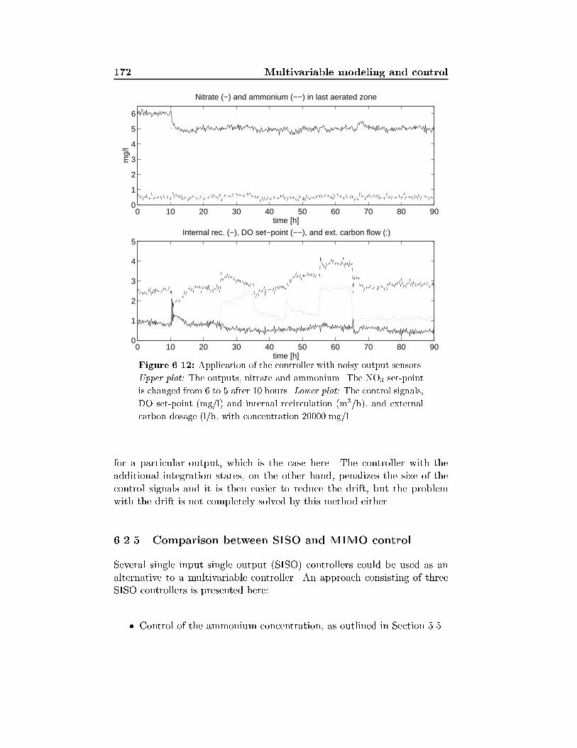
172 Multivariable modeling and control
0 10 20 30 40 50 60 70 80 900
1
2
3
4
5
6
time [h]
mg/
l
Nitrate (−) and ammonium (−−) in last aerated zone
0 10 20 30 40 50 60 70 80 900
1
2
3
4
5
time [h]
Internal rec. (−), DO set−point (−−), and ext. carbon flow (:)
Figure 6.12: Application of the controller with noisy output sensors.
Upper plot: The outputs, nitrate and ammonium. The NO3 set-point
is changed from 6 to 5 after 10 hours. Lower plot: The control signals,
DO set-point (mg/l) and internal recirculation (m3/h), and external
carbon dosage (l/h, with concentration 20000 mg/l.
for a particular output, which is the case here. The controller with theadditional integration states, on the other hand, penalizes the size of thecontrol signals and it is then easier to reduce the drift, but the problemwith the drift is not completely solved by this method either.
6.2.5 Comparison between SISO and MIMO control
Several single input single output (SISO) controllers could be used as analternative to a multivariable controller. An approach consisting of threeSISO controllers is presented here:
� Control of the ammonium concentration, as outlined in Section 5.5.
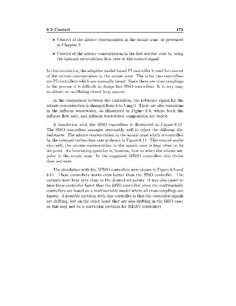
6.2 Control 173
� Control of the nitrate concentration in the anoxic zone, as presentedin Chapter 3.
� Control of the nitrate concentration in the last aerobic zone by usingthe internal recirculation ow rate as the control signal.
In this simulation, the adaptive model-based PI controller is used for controlof the nitrate concentration in the anoxic zone. The other two controllersare PI controllers which are manually tuned. Since there are cross couplingsin the process it is di�cult to design fast SISO controllers. It is very easyto obtain an oscillating closed loop system.
In the comparison between the controllers, the reference signal for thenitrate concentration is changed from 6 to 5 mg/l. There are also variationsin the in uent wastewater, as illustrated in Figure 6.9, where both thein uent ow rate, and in uent wastewater composition are varied.
A simulation with the SISO controllers is illustrated in Figure 6.13.The SISO controllers manages reasonably well to reject the di�erent dis-turbances. The nitrate concentration in the anoxic zone which is controlledby the external carbon ow rate is shown in Figure 6.14. This control worksalso well, the nitrate concentration in the anoxic zone is kept close to itsset-point. An interesting question is, however, how to select the nitrate set-point in the anoxic zone. In the suggested MIMO controllers this choicedoes not exist.
The simulation with the MIMO controllers were shown in Figure 6.8 and6.11. These controllers works even better than the SISO controller. Theoutputs ware kept very close to the desired set-points. It was also easier totune these controller faster than the SISO controller, since the multivariablecontrollers are based on a multivariable model where all cross-couplings areknown. A possible problem with this controller is that the controller signalsare drifting, but on the other hand they are also drifting in the SISO case,so this may not be a particular problem for MIMO controllers.
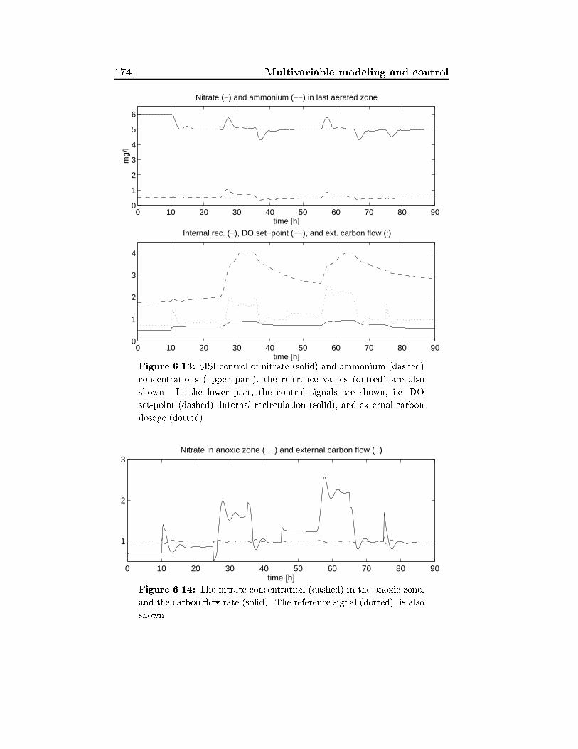
174 Multivariable modeling and control
0 10 20 30 40 50 60 70 80 900
1
2
3
4
time [h]
Internal rec. (−), DO set−point (−−), and ext. carbon flow (:)
0 10 20 30 40 50 60 70 80 900
1
2
3
4
5
6
time [h]
mg/
l
Nitrate (−) and ammonium (−−) in last aerated zone
Figure 6.13: SISI control of nitrate (solid) and ammonium (dashed)
concentrations (upper part), the reference values (dotted) are also
shown. In the lower part, the control signals are shown, i.e. DO
set-point (dashed), internal recirculation (solid), and external carbon
dosage (dotted).
0 10 20 30 40 50 60 70 80 90
1
2
3
time [h]
Nitrate in anoxic zone (−−) and external carbon flow (−)
Figure 6.14: The nitrate concentration (dashed) in the anoxic zone,
and the carbon ow rate (solid). The reference signal (dotted), is also
shown.
6.3 Some remarks 175
6.3 Some remarks
Tuning the LQ-controllers are relatively simple (easier than tuning a PIDcontroller). The elements in the R matrix (the Q matrix could also be used)are varied until the desired performance is obtained. To make the DO set-point, for example, smaller and less high frequent, the middle element inthe R-matrix is increased.
The presented controllers do not use measurements of the nitrate con-centration in the anoxic zone, and the air valve positions. It may hence bea good idea to extend the controller with these measurements, because ofthe following:
� If the nitrate concentration in the anoxic zone is close to zero, anincreased dosage of external carbon is not very useful.
� If an air valve has saturated, it is no point increasing (decreasing) theDO set-point.
One may argue if it is a good strategy or not to maintain a set-pointon the ammonium and nitrate concentration in the last aerated zone. It islikely that time-varying set-points are more optimal than constant ones. Ifa strategy for choosing the ammonium and nitrate set-points are derived,such a strategy may be applied to the multivariable controller.
A problem with the MIMO controllers is to �nd a good model of theprocess. Quite often a model is obtained which looks good in the validationfrom the identi�cation, but when it is used in the controller design, thecontroller does not work well. The derived controller tries to use a negativeinternal recirculation rate. Before MIMO control can be applied reliablyone has to �nd a method which can decide if an estimated model will workor not in a control design. One idea to solve this problem may be to studythe step responses for the di�erent input signals, and from this informationdecide if the model is suitable or not for controller design. Another problemis how to obtain a good model when you know the available model is notsuitable. A possible solution could be to discard data used in the subspaceidenti�cation, since this a�ects the estimated model. These problems are,however, topics for future research.
6.4 Conclusions
It has, by simulations, been shown that it is possible to estimate a lineartime-invariant state-space model, which well can predict the ammonium

176 Multivariable modeling and control
and nitrate concentration in the last aerated zone in a pre-denitrifyingactivated sludge process. The model uses the following six input signals:DO set-point, external carbon, internal recirculation, in uent ow, in uentcarbon and in uent ammonium.
Based on the estimated linear model, two multivariable linear quadratic(LQ) controller have been designed. The control strategy is based on main-taining the ammonium and the nitrate concentration in the last aeratedzone close to speci�ed set-points. The controllers use feedforward frommeasurable disturbances: in uent ow, in uent carbon and in uent am-monium. The controllers were evaluated in a simulation study. The �rstone was based on di�erentiating the system and deriving an incrementalcontroller. The second approach was to include additional integration statesfor each output. Both controllers showed high performance. It was, how-ever, found that the modeling part is crucial for the control performance.A further study of this aspect is an important topic for future research.

Chapter 7
Conclusions and topics for
future research
7.1 Conclusions
In this thesis some strategies to improve the control of wastewater treat-ment plants have been outlined. In particular control and estimation prob-lems in a pre-denitrifying activated sludge process have been studied. Byintroducing more advanced control, the e�uent concentrations of nitrate,ammonium, and oxygen consuming matter can be reduced. Less chemicalsand energy are also needed, which give a signi�cant economic incentive touse more advanced control strategies. The plant e�ciency and capacity canhence be improved.
By adding an external carbon dosage, the e�uent concentration of ni-trate can be reduced. Four types of controllers for the external carbondosage have been evaluated in a simulation study in Chapter 3. The controlstrategy was based on keeping the nitrate concentration in the anoxic zoneat a constant low level. The four controllers were a PI-controller, a gen-eralized minimum-variance adaptive controller, an adaptive LQ-controller,and a model-based adaptive PI controller. All controllers utilized feedfor-ward. The PID-controller may be hard to tune and its control performancedeteriorates when the process dynamic changes. The adaptive controllerswere easier to tune, and they also worked well. A safety net was, however,required to avoid numerical problems with the adaptive controllers. Themodel-based adaptive PI controller showed high performance, and it usesphysical knowledge of the process. The adaptive LQ-controller had alsohigh performance. The direct adaptive controller adapted fast to changes
178 Conclusions and topics for future research
in the process and was easy to implement. A practical experiment withthe direct adaptive controller has also been performed. It showed that thedirect adaptive controller could keep the nitrate concentration in the anoxiczone tight to a desired set-point.
In Chapter 4, on-line methods for estimating the time-varying respira-tion rate and the nonlinear oxygen transfer function were presented. Theestimator was based on a Kalman �lter approach where measurements ofthe dissolved oxygen concentration and the air ow rate were used. Twodi�erent models of the nonlinear KLa function were suggested: an expo-nential model and a cubic spline model. Two models for modeling thetime-varying respiration rate were also considered: a random walk modeland an integrated random walk model. An approach to estimate the oxy-gen transfer function by di�erentiating the data was also brie y outlined.The estimation procedures were illustrated both in a simulation study andon real data from a pilot plant. The results were successful both in the sim-ulation study and when applied to real data. In the practical experiment,the estimated respiration rate followed the measured respiration rate well.
The control of the dissolved oxygen in an activated sludge process wasdiscussed in Chapter 5. The basic idea was to explicitly take the nonlinearoxygen transfer function into account in the control design. Two designapproaches were then applied on the linearized process, pole-placementwith a PI-regulator and linear quadratic control with feedforward. In asimulation study, the performance of a linear and a nonlinear controller wasillustrated. It was shown that the nonlinear DO controller outperformed thelinear controller. The results from the simulation study were also con�rmedby experiments in a pilot plant. A set-point controller for the DO processwas outlined. The basic idea was to control the DO set-point so thatthe ammonium concentration in the last aerobic zone was kept low. Anexperiment in the pilot plant showed that, by using this controller not onlyenergy could be saved due to a lower DO set-point, but also the e�uentnitrate concentration became signi�cantly lower. A pressure controller wasalso evaluated in the pilot plant. The air pressure was controlled so thatthe most open valve was almost completely open.
In Chapter 6 it was shown, in simulations, that it was possible to esti-mate a linear time-invariant multivariable state-space model, which couldpredict the ammonium and nitrate concentration in the last aerated zonewell. This model was then used for design of multivariable LQ controllerswith feedforward. For the control, external carbon, internal recirculationrate, and DO set-point were considered as inputs. Ammonium and nitratein the last aerated zone were outputs. The controllers used feedforward
7.2 Topics for future research 179
from the measurable disturbances: in uent ow rate, in uent ammoniumconcentration and in uent substrate. Two di�erent controllers were evalu-ated in a simulation study. The �rst one was based on di�erentiating thesystem and deriving an incremental controller. The second approach wasto include additional integration states for each output. Both controllersshowed high performance. It was, however, found that the modeling partwas crucial for the control performance.
7.2 Topics for future research
7.2.1 Spatial DO control
It is possible to extend the set-point controller presented in Chapter 5in various respects, for example, to control the number of aerated zones.The order in which the aerated zones are switched o� may be important.Changing the aerobic/anoxic ratio also a�ects the dynamic in the nitri�-cation/denitri�cation processes. Ammonium and nitrate controllers mayhence need di�erent tuning for di�erent number of aerated zones. Place-ment of sensors may be another practical problem when changing an aerobiczone to an anoxic.
7.2.2 Further studies of the e�ect of surfactants
The surfactants have large impact on some WWTP. For example, it reducesthe KLa. When this happens the air ow rate have to be increased tomaintain the oxygen concentration, which consumes energy. If it is possibleto precipitate the surfactants this problem could be reduced. A controlstrategy for the surfactant could then be based on an estimated KLa.
Further studies are needed to determine if the surfactants deterioratethe sludge settling properties and sludge loss is obtained. If they do, it isanother reason to either try to �nd a precipitation chemical or make thepolluter reduce their use of surfactants.
7.2.3 Analyzing the information of the carbon dosage
Another topic for further research could be to analyze the additional infor-mation, as the variations in carbon ow rate may give. For example, theair ow rate gives some information about the organic load to the plant.The carbon ow rate could perhaps in a similar way be used to achieveinformation about the in uent wastewater composition, the denitri�cation
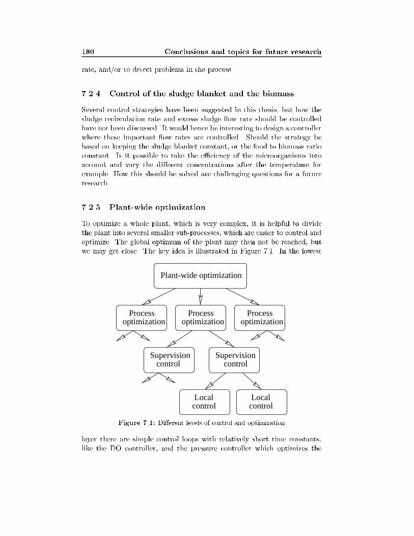
180 Conclusions and topics for future research
rate, and/or to detect problems in the process.
7.2.4 Control of the sludge blanket and the biomass
Several control strategies have been suggested in this thesis, but how thesludge recirculation rate and excess sludge ow rate should be controlledhave not been discussed. It would hence be interesting to design a controllerwhere these important ow rates are controlled. Should the strategy bebased on keeping the sludge blanket constant, or the food to biomass ratioconstant. Is it possible to take the e�ciency of the microorganisms intoaccount and vary the di�erent concentrations after the temperature forexample. How this should be solved are challenging questions for a futureresearch.
7.2.5 Plant-wide optimization
To optimize a whole plant, which is very complex, it is helpful to dividethe plant into several smaller sub-processes, which are easier to control andoptimize. The global optimum of the plant may then not be reached, butwe may get close. The key idea is illustrated in Figure 7.1. In the lowest
optimizationProcess
Plant-wide optimization
optimizationProcess Process
optimization
Supervisioncontrol
Supervisioncontrol
controlLocal
controlLocal
Figure 7.1: Di�erent levels of control and optimization
layer there are simple control loops with relatively short time constants,like the DO controller, and the pressure controller which optimizes the
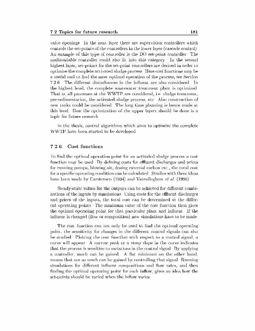
7.2 Topics for future research 181
valve openings. In the next layer there are supervision controllers whichcontrols the set-points of the controllers in the lower layer (cascade control).An example of this type of controller is the DO set-point controller. Themultivariable controller could also �t into this category. In the secondhighest layer, set-points for the set-point controllers are derived in order tooptimize the complete activated sludge process. Here cost functions may bea useful tool to �nd the most optimal operation of the process, see Section7.2.6. The di�erent disturbances in the in uent are also considered. Inthe highest level, the complete wastewater treatment plant is optimized.That is, all processes at the WWTP are considered, i.e. sludge treatment,pre-sedimentation, the activated sludge process, etc. Also construction ofnew tanks could be considered. The long time planning is hence made atthis level. How the optimization of the upper layers should be done is atopic for future research.
In the thesis, control algorithms which aims to optimize the completeWWTP have been started to be developed.
7.2.6 Cost functions
To �nd the optimal operation point for an activated sludge process a costfunction may be used. By de�ning costs for e�uent discharges and pricesfor running pumps, blowing air, dosing external carbon etc., the total costfor a speci�c operating condition can be calculated. Studies with these ideashave been made by Carstensen (1994) and Vanrolleghem et al. (1996).
Steady-state values for the outputs can be achieved for di�erent combi-nations of the inputs by simulations. Using costs for the e�uent dischargesand prices of the inputs, the total cost can be determined at the di�er-ent operating points. The minimum value of the cost function then givesthe optimal operating point for that particular plant and in uent. If thein uent is changed ( ow or composition) new simulations have to be made.
The cost function can not only be used to �nd the optimal operatingpoint, the sensitivity for changes in the di�erent control signals can alsobe studied. Plotting the cost function with respect to a control signal, acurve will appear. A narrow peak or a steep slope in the curve indicatesthat the process is sensitive to variations in the control signal. By applyinga controller, much can be gained. A at minimum on the other hand,means that not so much can be gained by controlling that signal. Runningsimulations for di�erent in uent compositions and ow rates, and then�nding the optimal operating point for each in ow, gives an idea how theset-points should be varied when the in ow varies.
182 Conclusions and topics for future research
There are, however, some problems with this approach.
� To be able to apply the strategy to a real wastewater treatment plant,a well calibrated model of the activated sludge process is needed. Thismay be hard to obtain.
� The method is based on steady-state values, exactly how the methodcould be extended to be valid for a dynamic system is not clear. Asimple idea could be to calculate the optimal steady-state operatingpoints for the changing in ow, and then low pass �lter these operatingpoints.
� The way to compute the optimal controller signal is very computa-tionally intense, if steady-state simulations should be used. Perhapsit is possible to �nd a less computationally intense method.
7.2.7 Extremum control
An alternative or modi�cation of the previous outlined method could beto use extremum control. The extremum controller has similarities withthe previous cost function approach, since it is also based on minimizinga cost function, but here real inputs and outputs will be used instead ofsimulated.
The idea is to de�ne a cost function J1 which is based on real costs ofrunning the plant. Assume then that J1 has an extremum point which, forexample, can be modeled by
J2 = UTAU +BTU + c
where U is the input vector which may consist of set-points, A is a coe�cientmatrix, B is a coe�cient vector, and c a scalar. A, B, and c could beestimated by an identi�cation method. The optimal control signal is thenfound by setting dJ2=dU = 0, which gives
u = �1
2A�1B
Exactly how this should work is a topic for future research, and there aresome open issues, e.g.
� The contents of U is not obvious. Which inputs should be included(maybe the cost function in Section 7.2.6 could answer that) shouldtime-lagged inputs be stored in the U vector.

7.2 Topics for future research 183
� Could J2 model the extremum point?
� Does there exist an extremum point.?
� How much excitation is needed to estimate A and B?

184 Conclusions and topics for future research

Appendix A
The generalized
minimum-variance controller
with feedforward
A.1 Derivation of the controller
The generalized minimum-variance controller, used to control the externalcarbon source in Chapter 3, is derived here.
Assume that the process to be controlled is described by the lineardiscrete-time model
A(q�1)y(t) = B(q�1)u(t�k)+D(q�1)w(t�d)+C(q�1) 1
�(q�1)e(t) (A.1)
where A(q�1), B(q�1), C(q�1) andD(q�1) are polynomials in the backwardshift operator q�1, with degrees na, nb, nc, and nd. The polynomialsA(q�1) and C(q�1) are monic, y(t) is the output and u(t) is the input.Furthermore, the time delays are denoted by k and d, and
�(q�1) = 1� q�1 (A.2)
The disturbance w(t) is measurable and the disturbance e(t) is unmeasur-able zero mean white noise.
The controller has the following stucture
(R(q�1) +�
r0C(q�1))�u(t) = �S(q�1)y(t)�Q(q�1)�w(t+ k � d) (A.3)

186 The generalized minimum-variance controller
To determine the controller polynomials, a predictor for the system(A.1) has to be determined. First y(t + k) is calculated from (A.1), itbecomes
y(t+ k) = qk�kB
Au(t) + qk�d
D
Aw(t) +
C
A�e(t+ k) (A.4)
The k-step predictor y(t+ kjt) is found by predicting the future noise sam-ples with their mean value, i.e. e(t + i) = 0, i > 0. It is hence desired topartition C
A�e(t + k) into two parts. One part which contains the futurenoise and one which contains the old noise. This can be done by
C
A�= F + q�k
G
A�(A.5)
where F and G are polynomials determined by (A.5) with the degreesdeg(F )=k� 1 and deg(G)=max(deg(�A),deg(C))� 1. F and G are deter-mined by carrying out the polynomial division C
A� .
Using (A.5) in (A.4) with the future noise equal to zero gives the pre-dictor
y(t+ kjt) = B
Au(t) + qk�d
D
Aw(t) +
G
A�e(t) (A.6)
This predictor contains e(t), which can be expressed in terms of y(t), u(t),and w(t) by using (A.1). Inserting the expression of e(t) in (A.6) gives the�nal predictor
y(t+ kjt) = qk�kBF
C�u(t) + qk�d
DF
C�w(t) +
G
Cy(t) (A.7)
The k-step predictor (A.7) can be found in e.g. �Astr�om and Wittenmark(1990) except for the extra term qk�dDF=C�w(t) which has been includedto account for the measurable disturbance.
To �nd the control law which minimizes the criterion (see also Clarkeand Gawthrop (1975))
J =1
2E[y2(t+ k) + �(�u(t))2jYt] (A.8)
we �rst notice that
y(t+ k) = y(t+ kjt) + Fe(t+ k) (A.9)
The incremental control signal �u(t), which gives the minimum value of Jis found by setting the derivative of J with respect to �u(t) to zero.
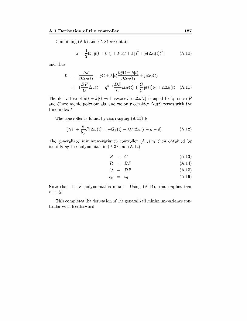
A.1 Derivation of the controller 187
Combining (A.9) and (A.8) we obtain
J =1
2E[(y(t+ kjt) + Fe(t+ k))2 + �(�u(t))2] (A.10)
and thus
0 =@J
@�u(t)= y(t+ kjt)@y(t+ kjt)
@�u(t)+ ��u(t)
= (BF
C�u(t) + qk�d
DF
C�w(t) +
G
Cy(t))b0 + ��u(t) (A.11)
The derivative of y(t + kjt) with respect to �u(t) is equal to b0, since Fand C are monic polynomials, and we only consider �u(t) terms with thetime index t.
The controller is found by rearranging (A.11) to
(BF +�
b0C)�u(t) = �Gy(t)�DF�w(t+ k � d) (A.12)
The generalized minimum-variance controller (A.3) is then obtained byidentifying the polynomials in (A.3) and (A.12).
S = G (A.13)
R = BF (A.14)
Q = DF (A.15)
r0 = b0 (A.16)
Note that the F polynomial is monic. Using (A.14), this implies thatr0 = b0.
This completes the derivation of the generalized minimum-variance con-troller with feedforward.

188 The generalized minimum-variance controller
Appendix B
LQ-control with feedforward
The aim of linear quadratic (LQ) controller design is to �nd a controllerwhich minimizes the sum of the variance of the output and the weightedvariance of the input, see �Astr�om and Wittenmark (1990).
When a measurable disturbance exists, a feedback controller can becomplemented with disturbance measurement feedforward, see e.g. Ster-nad and S�oderstr�om (1988) and Grimble (1988). For a given degree ofdisturbance rejection, the high frequency gain of the feedback controllercan then be reduced, which may increase the stability robustness, see Ster-nad (1991).
The LQ-controller derived here makes it possible to use separate penal-ties on the contributions to the control signal from measurable and unmea-surable disturbances. This makes it for example possible to use a controllerwith deadbeat feedforward in combination with a cautious feedback. Thefeedforward does not a�ect the closed-loop stability. It may therefore beuseful to apply a smaller penalty on the control signal generated by thefeedforward than on the feedback. Separate control penalties may also befruitful, when the variance of the measurement noise on the feedforwardsensor is di�erent compared to the feedback sensor, see also e.g. Grimble(1988).
190 LQ-control with feedforward
B.1 The LQ problem
Assume that the process to be controlled is described by the linear discrete-time model
A(q�1)y(t) = B(q�1)u(t�k)+D(q�1)w(t�d)+C(q�1) 1
�(q�1)e(t) (B.1)
where A(q�1), B(q�1), C(q�1) andD(q�1) are polynomials in the backwardshift operator q�1, with degrees na, nb, nc, nd. The polynomials A(q�1)and C(q�1) are monic, y(t) is the output and u(t) is the input. Furthermore,the time delays are denoted by k and d, and
�(q�1) = 1� q�1 (B.2)
The disturbance w(t) is measurable and the disturbance e(t) is unmeasur-able zero mean white noise. The measurable disturbance w(t) is modelledby an ARMA process
w(t) =G(q�1)
H(q�1)v(t) (B.3)
where v(t) is zero mean white noise. The polynomials G(q�1) and C(q�1)are required to be stable polynomials1. A stable polynomial is de�ned as apolynomial which has all its zeros inside the the unit circle.
A frequently used criterion in LQ-design, see e.g. �Astr�om and Witten-mark (1990) is
J = limN!1
1
N
NXt=0
[Ey(t)2 + �Eu(t)2] (B.4)
It is also common that, instead of penalizing the variance of the controlsignal u(t) as in the criterion (B.4), the variance of
�u(t) = u(t)� u(t� 1) (B.5)
is penalized instead. This allows the control signal to drift while the vari-ations of the control signal are reduced. The choice of penalizing �u(t)instead of u(t), is reasonable when there are drifting disturbances, sincesuch disturbances require a drifting control signal, which forces the con-troller to contain integration2. The LQ controller to be derived here will
1If G or C are estimated, and zeros in jzj � 1 are obtained, these zeros then haveto be projected into the stable region. Such a projection does not change the spectraldensity of Gv(t) or Ce(t).
2If the control signal is drifting, the problem of minimizing the criterion (B.4) wouldbe unsolvable when penalizing u(t) since the criterion grows to in�nity for drifting signals.
B.1 The LQ problem 191
therefore use �u in the criterion. The obtained integrating controller is alsoadvantageous for other reasons, e.g. it makes the controller less sensitive tolow-frequency modelling errors.
To derive a LQ-controller where it is possible to use separate penaltieson components of the control signal which originate from di�erent distur-bances, the control signal increment is partitioned as
�u(t) = �ue(t) + �uv(t) (B.6)
where ue(t) is the part of the control signal which is generated by the un-measurable noise e(t), and uv(t) is the part originating from the innovationsequence of the measurable disturbance v(t). The new criterion with twopenalty parameters is
J = limN!1
1
N
NXt=0
[Ey(t)2 + E(p�e�ue(t) +
p�v�uv(t))
2] (B.7)
The q�1 argument is for simplicity skipped in most of the following polyno-mial equations. The polynomial A(q�1), for example will only be denotedby A, and so on. Conjugated polynomials are also used. They are denotedby a � and de�ned as follows. If
B(q�1) = b0 + b1q�1 + b2q
�2 + : : : (B.8)
thenB�(q) = b0 + b1q + b2q
2 + : : : (B.9)
If B(q�1) is a stable polynomial, then B�(q) is unstable.
The controller minimizing the criterion (B.7) is presented in the follow-ing Theorem.
Theorem B.1 Consider the system (B.1), and assume A� and B to have
no common unstable factors. The controller which minimizes the criterion
(B.7), where v(t) and e(t) are assumed to be uncorrelated, is then given by
R(q�1)�u(t) = �S(q�1)y(t)� Q(q�1)
P (q�1)w(t) (B.10)
where R(q�1), S(q�1), P (q�1) and Q(q�1) are controller polynomials.
The feedback polynomials R(q�1) and S(q�1) are determined by the
unique solution of the pole placement equation
��= AR�+ q�kBS = �eC (B.11)
192 LQ-control with feedforward
when A� and B have no common factors. If they have common factors,
then see remark 2. In (B.11) re is a scalar and �e(q�1) is a stable monic
polynomial derived from the spectral factorization
re�e��e = BB� + �eA��
�A� (B.12)
The feedforward �lter denominator P (q�1) is determined by
P = G�v (B.13)
where �v(q�1) is a stable monic polynomial derived from the spectral fac-
torization
rv�v��v = BB� + �vA��
�A� (B.14)
The feedforward polynomial Q(q�1) is found as the unique solution of the
linear polynomial equation
(RB� � �v��A�Sq�k)q�d+kDG� = rv�
�vQ+ qL��H (B.15)
with respect to Q(q�1) and L�(q�1).
Proof: The proof is given in Lindberg (1995).
Remark 1: As mentioned before, the control signal has been separatedinto two parts ue(t) and uv(t) which can be penalized separately. Oneshould, however, be aware of the following property. Since uv(t) is derivedfrom the measurable disturbance v(t), a large value of �v implies that v(t)will not be rejected, not even by the feedback loop. The e�ect of the mea-surable disturbance v(t) on the feedback signal will in such a case insteadbe (partly) cancelled by the feedforward control signal. In general onewould like a slow feedback for stability reasons and a fast feedforward toreject measurable disturbances fast, then �e > �v and this property doesnot occur.
Remark 2: When A� and B have common factors, the feedback poly-nomials R(q�1) and S(q�1) are determined by the unique solution to thecoupled linear polynomial equations
�e��A�C + q�k+1BX� = re�
�eR (B.16)
qkCB� � qA�X� = re��eS (B.17)
with respect to R(q�1), S(q�1) and X�(q).
Remark 3: When � = �e = �v, a special and simpli�ed case is ob-tained, where the feedforward polynomials P (q�1) and Q(q�1) instead are
B.1 The LQ problem 193
determined by the following equations:
P = G (B.18)
q�d+1DG�X� = r��Q+ qL�CH (B.19)
where the X�(q�1) polynomial is obtained from either (B.16) or (B.17).
The degrees of the Q and L polynomials should here be chosen as
nQ = max(nd + ng + d+ 1; nc + nh)� 1 (B.20)
nL = max(0; k � d) + n� � 1 (B.21)
The feedback polynomials are not a�ected. When �e 6= �v the degrees ofthe polynomials are derived as in Section B.1.1.
Remark 4: Typical selection of �e and �v. The most useful applicationof this controller is to design the feedforward loop faster than the feedback.Since the feedforward does not a�ect the closed-loop stability it is useful toapply a smaller penalty on the control signal generated by the feedforward(�v) than on the feedback (�e).
Remark 5: When the measurable disturbance w(t) is drifting, i.e. whena factor � exists in the denominator of the model (B.3) of w(t)
w(t) =G
�H1v(t)
H = �H1
then (B.15) has to be slightly modi�ed. Otherwise � becomes a commonfactor of both sides of the equation. To see this, we notice that � is a factorof the left-hand side of (B.15) and in one of the right-hand side terms (H).Then � must also be a factor of Q, if the equation is to have a solution.To avoid this problem, we explicitly introduce � as a factor in Q, as
Q = �Q1 (B.22)
and cancel this factor everywhere in (B.15). Equation (B.15) is then re-duced to
(RB� � �v��A�Sz�k)z�d+kDG = rv�
�vQ1 + zL��H1 (B.23)
and can now be solved with respect to Q1, de�ned in (B.22). As noted inSternad (1991), the same type of modi�cation must be applied to (B.19).
In Figure B.1 the process with the controller is illustrated. Note that1=(R(q�1)�(q�1)) is present in both the feedback and the feedforward loop.
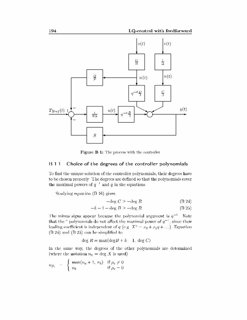
194 LQ-control with feedforward
m m
QP
1R� q�k B
A
?-
6
- - - -
�S
q�d DA
CA
1�
GH
����HHHj
?
�
?
? ?
�
�+
n(t)
e(t)v(t)
y(t)u(t)
w(t)
Tyref (t)
Figure B.1: The process with the controller
B.1.1 Choice of the degrees of the controller polynomials
To �nd the unique solution of the controller polynomials, their degrees haveto be chosen properly. The degrees are de�ned so that the polynomials coverthe maximal powers of q�1 and q in the equations.
Studying equation (B.16) gives
�deg C � �deg R (B.24)
�k + 1� deg B � �deg R (B.25)
The minus signs appear because the polynomial argument is q�1. Notethat the � polynomials do not a�ect the maximal power of q�1, since theirleading coe�cient is independent of q (e.g. X� = x0+ x1q+ : : :). Equation(B.24) and (B.25) can be simpli�ed to
deg R = max(degB + k � 1; deg C)
In the same way, the degrees of the other polynomials are determined(where the notation nx = deg X is used)
n�e =
(max(na + 1; nb) if �e 6= 0nb if �e = 0
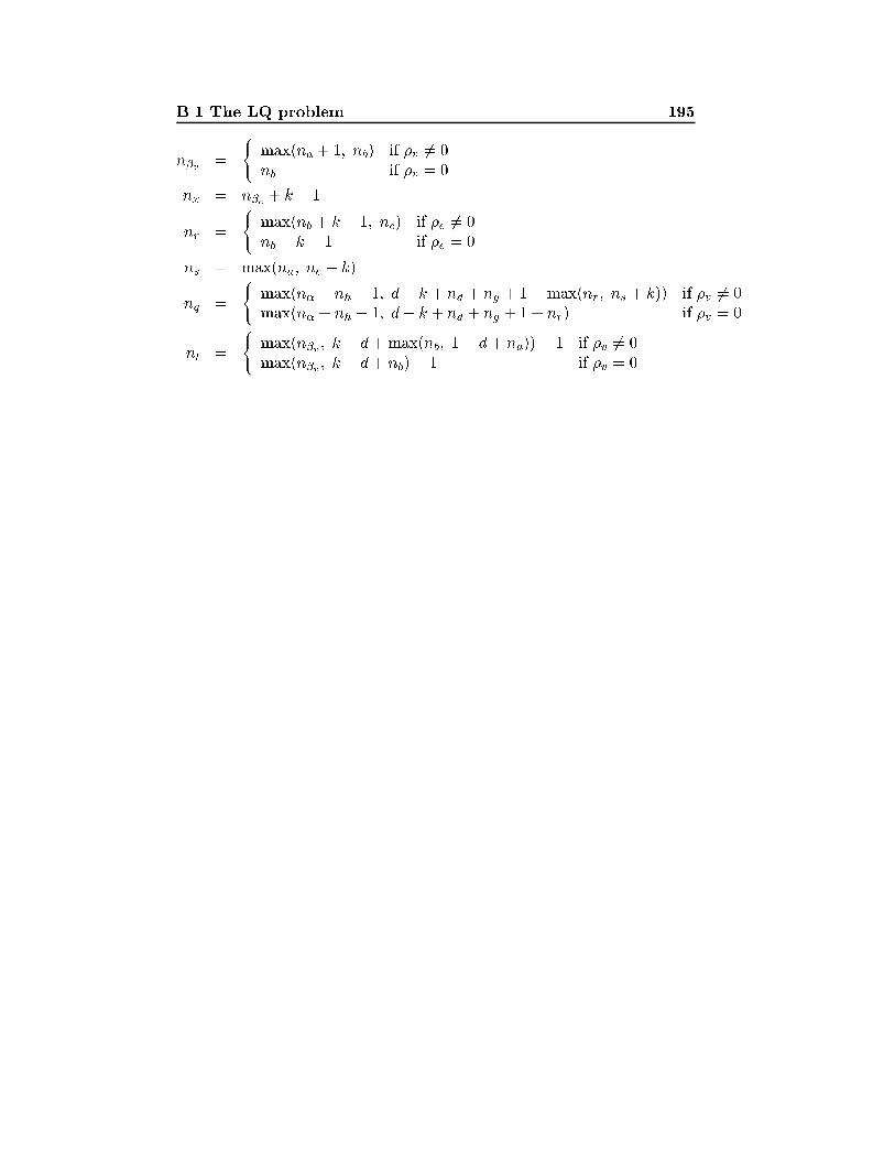
B.1 The LQ problem 195
n�v =
(max(na + 1; nb) if �v 6= 0nb if �v = 0
nx = n�e + k � 1
nr =
(max(nb + k � 1; nc) if �e 6= 0nb + k � 1 if �e = 0
ns = max(na; nc � k)
nq =
(max(n� + nh � 1; d� k + nd + ng + 1 +max(nr; ns + k)) if �v 6= 0max(n� + nh � 1; d� k + nd + ng + 1 + nr) if �v = 0
nl =
(max(n�v ; k � d+max(nb; 1� d+ na))� 1 if �v 6= 0max(n�v ; k � d+ nb)� 1 if �v = 0

196 LQ-control with feedforward
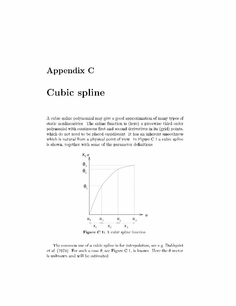
Appendix C
Cubic spline
A cubic spline polynomial may give a good approximation of many types ofstatic nonlinearities. The spline function is (here) a piecewise third orderpolynomial with continuous �rst and second derivatives in its (grid) points,which do not need to be placed equidistant. It has an inherent smoothnesswhich is natural from a physical point of view. In Figure C.1 a cubic splineis shown, together with some of the parameter de�nitions.
uuu 1 2 3
u
1
3
2
x xx1 2 3
L
u0
K a
θθ
θ
Figure C.1: A cubic spline function.
The common use of a cubic spline is for interpolation, see e.g. Dahlquistet al. (1974). For such a case �, see Figure C.1, is known. Here the � vectoris unknown and will be estimated.
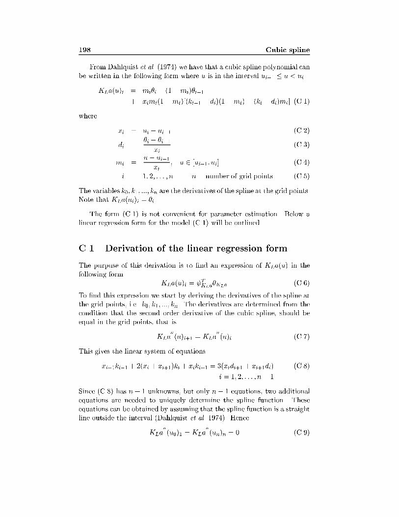
198 Cubic spline
From Dahlquist et al. (1974) we have that a cubic spline polynomial canbe written in the following form where u is in the interval ui�1 � u < ui
KLa(u)i = mi�i + (1�mi)�i�1
+ ximi(1�mi)[(ki�1 � di)(1�mi)� (ki � di)mi] (C.1)
where
xi = ui � ui�1 (C.2)
di =�i � �i�1
xi(C.3)
mi =u� ui�1
xi; u 2 [ui�1; ui] (C.4)
i = 1; 2; : : : ; n n = number of grid points (C.5)
The variables k0; k1; :::; kn are the derivatives of the spline at the grid points.Note that KLa(ui)i = �i.
The form (C.1) is not convenient for parameter estimation. Below alinear regression form for the model (C.1) will be outlined.
C.1 Derivation of the linear regression form
The purpuse of this derivation is to �nd an expression of KLa(u) in thefollowing form.
KLa(u)i = TKLa�KLa (C.6)
To �nd this expression we start by deriving the derivatives of the spline atthe grid points, i.e. k0; k1; :::; kn. The derivatives are determined from thecondition that the second order derivative of the cubic spline, should beequal in the grid points, that is
KLa00
(u)i+1 = KLa00
(u)i (C.7)
This gives the linear system of equations
xi+1ki�1 + 2(xi + xi+1)ki + xiki+1 = 3(xidi+1 + xi+1di) (C.8)
i = 1; 2; : : : ; n� 1
Since (C.8) has n+ 1 unknowns, but only n� 1 equations, two additionalequations are needed to uniquely determine the spline function. Theseequations can be obtained by assuming that the spline function is a straightline outside the interval (Dahlquist et al. 1974). Hence
KLa00
(u0)1 = KLa00
(un)n = 0 (C.9)
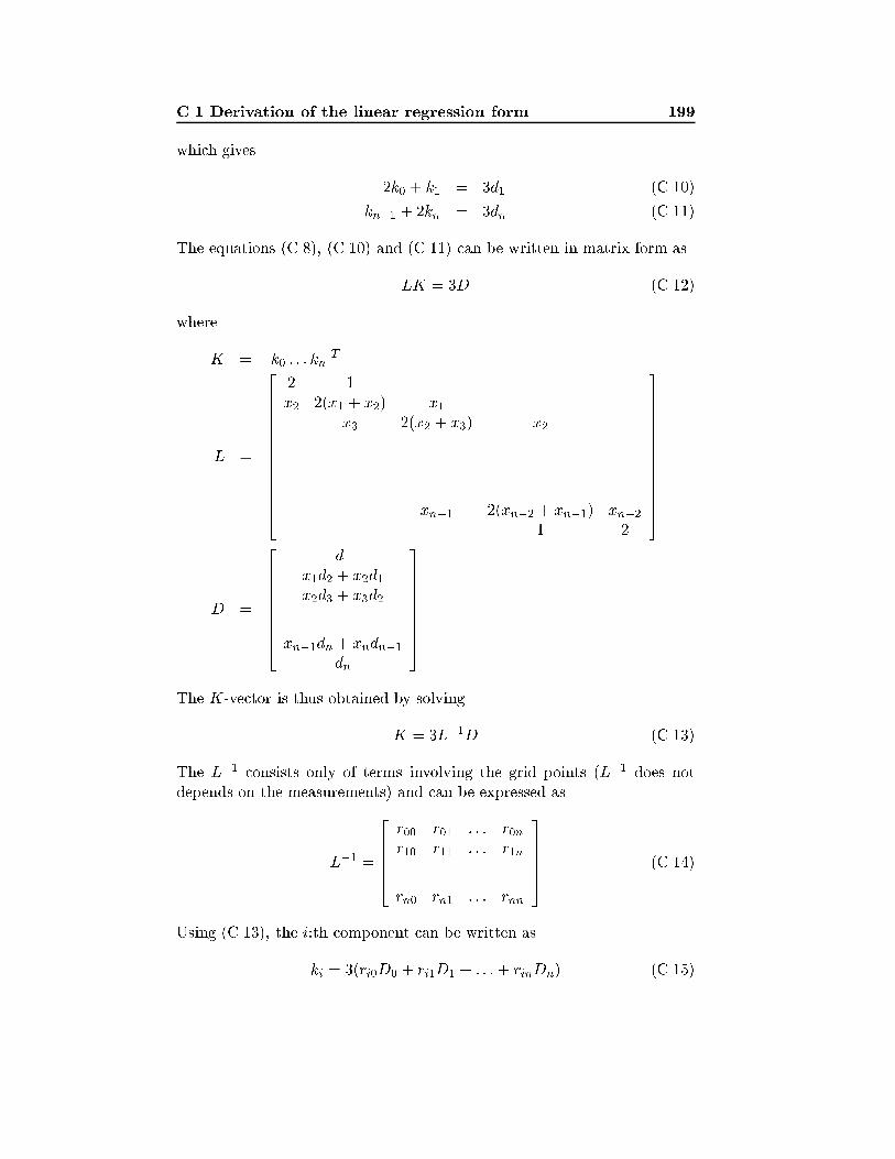
C.1 Derivation of the linear regression form 199
which gives
2k0 + k1 = 3d1 (C.10)
kn�1 + 2kn = 3dn (C.11)
The equations (C.8), (C.10) and (C.11) can be written in matrix form as
LK = 3D (C.12)
where
K = [k0 : : : kn]T
L =
266666666666664
2 1x2 2(x1 + x2) x1
x3 2(x2 + x3) x2
. . .. . .
. . .
xn�1 2(xn�2 + xn�1) xn�21 2
377777777777775
D =
2666666664
d1x1d2 + x2d1x2d3 + x3d2
...xn�1dn + xndn�1
dn
3777777775The K-vector is thus obtained by solving
K = 3L�1D (C.13)
The L�1 consists only of terms involving the grid points (L�1 does notdepends on the measurements) and can be expressed as
L�1 =
266664r00 r01 : : : r0nr10 r11 : : : r1n...
......
rn0 rn1 : : : rnn
377775 (C.14)
Using (C.13), the i:th component can be written as
ki = 3(ri0D0 + ri1D1 + : : :+ rinDn) (C.15)
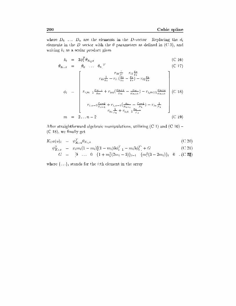
200 Cubic spline
where D0 : : : Dn are the elements in the D-vector. Replacing the dielements in the D vector with the � parameters as de�ned in (C.3), andwriting ki as a scalar product gives
ki = 3�Ti �KLa (C.16)
�KLa = [�0 : : : �n]T (C.17)
�i =
26666666666664
�ri0 1x1� ri1
x2x1
ri01x1
+ ri1(x2x1� x1
x2)� ri2
x3x2
...ri;m�1
xm�1
xm+ rim(
xm+1
xm� xm
xm+1)� ri;m+1
xm+2
xm+1
...ri;n�2
xn�2
xn�1+ ri;n�1(
xnxn�1
� xn�1
xn)� rin
1xn
rin1xn
+ ri;n�1xn�1
xn
37777777777775(C.18)
m = 2 : : : n� 2 (C.19)
After straightforward algebraic manipulations, utilizing (C.1) and (C.16) {(C.18), we �nally get
KLa(u)i = TKLa�KLa (C.20)
TKLa= ximi(1�mi)[(1 �mi)3�
Ti�1 �mi3�
Ti ] +G (C.21)
G = [0 : : : 0 f1 +m2i (2mi � 3)gi�1 fm2
i (3� 2mi)gi 0 : : : 0](C.22)
where f: : :gi stands for the i:th element in the array.
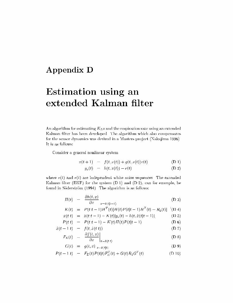
Appendix D
Estimation using an
extended Kalman �lter
An algorithm for estimatingKLa and the respiration rate using an extendedKalman �lter has been developed. The algorithm which also compensatesfor the sensor dynamics was derived in a Masters project (Nakajima 1996).It is as follows:
Consider a general nonlinear system
x(t+ 1) = f(t; x(t)) + g(t; x(t))v(t) (D.1)
ys(t) = h(t; x(t)) + e(t) (D.2)
where v(t) and e(t) are independent white noise sequences. The extendedKalman �lter (EKF) for the system (D.1) and (D.2), can for example, befound in S�oderstr�om (1994). The algorithm is as follows:
H(t) =@h(t; x)
@x
����x=x(tjt�1)
(D.3)
K(t) = P (tjt� 1)HT (t)[H(t)P (tjt� 1)HT (t) +R2(t)]�1(D.4)
x(tjt) = x(tjt� 1) +K(t)[ys(t)� h(t; x(tjt� 1))] (D.5)
P (tjt) = P (tjt� 1)�K(t)H(t)P (tjt� 1) (D.6)
x(t+ 1jt) = f(t; x(tjt)) (D.7)
FE(t) =@f(t; x)
@x
����x=x(tjt)
(D.8)
G(t) = g(t; x)jx=x(tjt) (D.9)
P (t+ 1jt) = FE(t)P (tjt)F TE (t) +G(t)R1G
T (t) (D.10)
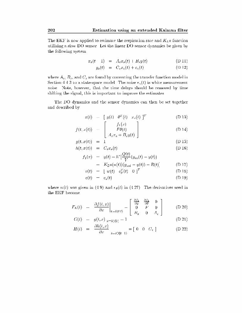
202 Estimation using an extended Kalman �lter
The EKF is now applied to estimate the respiration rate and KLa functionutilizing a slow DO sensor. Let the linear DO sensor dynamics be given bythe following system
xs(t+ 1) = Asxs(t) +Bsy(t) (D.11)
ys(t) = Csxs(t) + es(t) (D.12)
where As, Bs, and Cs are found by converting the transfer function model inSection 4.4.3 to a state-space model. The noise es(t) is white measurementnoise. Note, however, that the time delays should be removed by timeshifting the signal, this is important to improve the estimates.
The DO dynamics and the sensor dynamics can then be set togetherand described by
x(t) = [ y(t) �T (t) xs(t) ]T (D.13)
f(t; x(t)) =
264 f1(x)F�(t)
Asxs +Bsy(t)
375 (D.14)
g(t; x(t)) = 1 (D.15)
h(t; x(t)) = Csxs(t) (D.16)
f1(x) = y(t) + h�[Q(t)
V(yin(t)� y(t))
+ KLa(u(t))(ysat � y(t))�R(t)] (D.17)
v(t) = [ w(t) eT� (t) 0 ]T (D.18)
e(t) = es(t) (D.19)
where w(t) was given in (4.9) and e�(t) in (4.27). The derivatives used inthe EKF become
FE(t) =@f(t; x)
@x
����x=x(tjt)
=
264@f1@y
@f1@�
0
0 F 0Bs 0 As
375 (D.20)
G(t) = g(t; x)jx=x(tjt) = 1 (D.21)
H(t) =@h(t; x)
@x
����x=x(tjt�1)
= [ 0 0 Cs ] (D.22)
Bibliography
Ahl�en, A. and M. Sternad (1988). Introduction to Adaptive control. Systemsand Control Group, Uppsala University. (In Swedish).
Ahl�en, A. and M. Sternad (1989). Optimal deconvolution based on poly-nomial methods. IEEE Trans. on Acoustics, Speech, and Signal Pro-
cessing 37(2), 217 { 226.
Akaike, H. (1981). Modern development of statistical methods. In: Trendsand Progress in System Identi�cation (P. Eykho�, Ed.). PergamonPress.
Andersson, B., U. Nyberg and H. Aspegren (1995). Methanol and ethanolas external carbon sources for denitri�cation. Nordic Seminar: Espoo,Finland.
Andersson, C. and Y. Lundberg (1995). Addition of weighting agents fore�ectivisation of the activated sludge process. Master's thesis. Dep. ofWater Resources Engineering, Royal Institute of Technology, Sweden.(In Swedish).
Andrews, J. F. (1994). Dynamic control of wastewater treatment plants.Environ. Sci. Technol. 28(9), 434 { 440.
Aspegren, H., B. Andersson, U. Nyberg and J. la Cour Jansen(1992). Model and sensor based optimization of nitrogen removal atKlagshamn wastewater treatment plant.Wat. Sci. Tech. 26(5{6), 1315{ 1323.
�Astr�om, K. J. and B. Wittenmark (1989). Adaptive Control. Addison-Wesley, Reading, Massachusetts.
�Astr�om, K. J. and B. Wittenmark (1990). Computer-Controlled Systems.Prentice-Hall International Editions, Inc. Englewood Cli�s.
204 BIBLIOGRAPHY
�Astr�om, K. J. and J. Nilsson (1994). Analysis of a scheme for iteratedidenti�cation and control. SYSID 1994 Copenhagen, Denmark.
�Astr�om, K. J. and T. H�agglund (1984). Automatic tuning of simple regula-tors with speci�cations on phase and amplitude margins. Automatica20(5), 645{651.
Balm�er, P. and B. Hultman (1988). Control of phosphorus discharges:present situation and trends. Hydrobiologia 170, 305{319.
Barnes, D. and P. J. Bliss (1983). Biological Control of Nitrogen in Wastew-
ater Treatment. E. & F. N. Spon, London & New York.
Bastin, G. and D. Dochain (1990). On-line Estimation and Adaptive Con-
trol of Bioreactors. Elsevier, Amsterdam.
Behse, W. (1995). Nitrogen removal, process evaluation of the wtp in upp-sala. Technical Report Mat.nr: 2447. Dept. of Water Resources Eng.,Royal Institute of Technology. Stockholm, Sweden.
Bennett, G. F. (1980). Oxygen transfer rates, mechanisms, and applica-tions in biological wastewater treatment. Critical Rev. in Env. Control
pp. 301{391.
Bergh, S-G. (1996). Diagnosis problems in wastewater settling. Licentiatethesis. Lund Institute of Technology. Dept. of Industrial Electrical Eng.and Automation. CODEN:LUTEDX/(TEIE-1011)/1-118/(1996).
Bocken, S. M., M. Braae and P. L. Dold (1989). Dissolved oxygen con-trol and oxygen utilization rate estimation: Extension of the holm-berg/olsson method. Wat. Sci. Tech. 21, 1197{1208.
Bradley, J. W., S. Kyosai, P. Matthews, K. Sato and M Webber (1992).Worldwide sludge management practices. In: Municipal Sewage Sludge
Management: Processing, Utilization and Disposal (C. Lue-Hing, D. R.Zenz and R. Kuchenrither, Eds.). Technomic publishing company, Inc.,Lancaster, USA.
Brenner, A. (1991). External carbon, additional reactor { To add or not toadd?. Interactions of wastewater biomass and reactor con�gurationsin biological treatment plants 21{23 August, Copenhagen, Denmark.
Carlsson, B. (1993). On-line estimation of the respiration rate in an acti-vated sludge process. Wat. Sci. Tech. 28(11{12), 427{434.
Carlsson, B. (1995). Automatic control in wastewater treatment plants.Cirkulation (6), {. (In Swedish).
BIBLIOGRAPHY 205
Carlsson, B. (1997). The use of automatic control in wastewater treamentplants. Nordisk konferens, kv�averening och biologisk fosfor rening,Stockholm 20-30 Jan.
Carlsson, B. and C-F. Lindberg (1995). A control and supervision systemfor an activated sludge pilot plant. Ninth Forum for Applied Biotech-nology, 27{29 Sept. pp 2491{2494.
Carlsson, B. and S. Hasselblad (1996). A process simulator for the activatedsludge process. Cirkulation (5), {. (In Swedish).
Carlsson, B. and T. Wigren (1993). On-line identi�cation of the dissolvedoxygen dynamic in an activated sludge process. 12th World Congressof IFAC, Sydney, Australia, July 19-23.
Carlsson, B., C-F. Lindberg, S. Hasselblad and S. Xu (1994a). On-lineestimation of the respiration rate and the oxygen transfer rate atKungs�angen wastewater plant in Uppsala.Wat. Sci. Tech. 30(4), 255{263.
Carlsson, B., J. Latomaa and C-F. Lindberg (1994b). A control andsupervision system for an activated sludge process (ett styr- och�overvakningssytem f�or en aktivslamprocess. Reglerm�ote '94, 25{26Oct. V�aster�as, Sweden.
Carlsson, B., S. Hasselblad, E. Plaza, S. M�artensson and C-F. Lindberg(1997). Design and operation of a pilot-scale activated sludge plant.Vatten 53(1), 27{32.
Carstensen, J. (1994). Identi�cation of wastewater processes. PhD thesis.IMSOR & I. Kr�uger Systems AS, Lyngby, Denmark.
Clarke, D. W. and P. J. Gawthrop (1975). Self-tuning controller. Proc. IEE122, 929{934.
Cook, S. C. and P. W. Jowitt (1985). Investigation of dissolved oxygen dy-namics in the activated sludge process. IFAC Identi�cation and SystemParameter Estimation pp. 241{248. York, UK.
Coury, B. G. (1996). Water level control for the toilet tank: A historicalperspective. In: The Control Handbook (W. S. Levine, Ed.). CRCPress, Inc., Boca Raton, USA.
Dahlquist, G., �A Bj�orck and N. Andersson (1974). Numerical Methods.Prentice-Hall.
206 BIBLIOGRAPHY
Dochain, D. and M. Perrier (1993). Control design for nonlinear wastewatertreatment processes. Wat. Sci. Tech. 28(11{12), 283.
Doyle, J. C. and G. Stein (1979). Robustness with observers. IEEE Trans.
on Automatic Control AC{24(4), 607{611.
Elmqvist, H., K. J. �Astr�om and T. Sch�onthal (1986). Simnon-User's Guidefor MS-DOS Computers. Dept. of Automatic Control, Lund Inst. ofTechn., Sweden.
EPA (1989). Fine Pore Aeration Systems. United States EnvironmentalProtection Agency, EPA/625/1-89/023.
Finnson, A. (1994). Computer simulations of full-scale activated sludgeprocesses. Licentiate thesis. Royal Institute of Technology. Departmentof Water Resources Eng. TRITA-VAT 1941, Stockholm Sweden.
Flanagan, M.J., B.D. Bracken and J.F. Roesler (1977). Automatic dissolvedoxygen control. Journal of the Environmental Engineering Division
EE4, 707{722.
Garc��a, C. E., D. M. Prett and M. Morari (1989). Model predictive control:Theory and practice { a survey. Automatica 25(3), 335{348.
Grijspeerdt, K., P. Vanrolleghem and W. Verstraete (1995). Selection ofone-dimensional sedimentation models for on-line use. Wat. Sci. Tech.
31(2), 193{204.
Grimble, M. J. (1988). Two-degrees of freedom feedback and feedfor-ward optimal control of multivariable stochastic systems. Automatica24(6), 809{817.
Gustafsson, L-G., D. Lumley, C. Lindeborg and J. Haraldsson (1993). In-tegrating a catchment simulator into wastwater treatment plant oper-ation. Wat. Sci. Tech. 28(11{12), 45{54.
Gustafsson, T. (1988). Regsim. LUG Elektronik HB, Lule�a, Sweden.
Hallin, S. and M. Pell (1996). Denitri�cation in activated sludge withexternal carbon sources { perspectives and consequences. Vatten
52(3), 213{216. (In Swedish).
Hallin, S., C-F. Lindberg, M. Pell, E. Plaza and B. Carlsson (1996). Micro-bial adaptation, process performance and a suggested control strategyin a pre-dentrifying system with ethanol dosage.Wat. Sci. Tech. 34(1{2), 91{99.

BIBLIOGRAPHY 207
Harremo�es, P., M. Henze, E. Arvin and E. Dahi (1994). Teoretisk Vandhy-giejne. Polyteknisk Forlag, Lyngby, Denmark.
Hasselblad, S. and S. Hallin (1996). Intermittent dosage of ethanol in a pre-denitrifying activated sludge process. Wat. Sci. Tech. 34(1{2), 387{389.
Hellstr�om, B. G. and J. Bosander (1990). Styrstrategier av tillsats av externkolk�alla vid f�ordenitri�kation. SYVAB, Himmerfj�ardsverket, Sweden.
Henze, M., C. P. L. Grady Jr., W. Gujer, G. v. R. Marais and T. Matsuo(1987). Activated sludge model no. 1. Scienti�c and Technical Report
No. 1. IAWQ, London, Great Britain.
Henze, M., P. Harremo�es, J. la Cour Jansen and E. Arvin (1995a).Wastewater treatment, biological and chemical processes. Springer-Verlag Berlin Heidelberg, Germany.
Henze, M., W. Gujer, T. Mino, T. Matsuo, M. C. Wentzel and G. v. R.Marais (1995b). Activated sludge model no. 2. Scienti�c and TechnicalReport No. 3. IAWQ, London, Great Britain.
Holmberg, A. (1981). Microprocessor-based estimation of oxygen utilizationin the activated sludge wastewater treatment process. Int. J. SystemsSci. 12(6), 703{718.
Holmberg, U. (1990). On the identi�ability of dissolved oxygen concentra-tion dynamics. IAWPRC's 25th Anniversary Conference and Exhibi-tion, Kyoto, Japan.
Holmberg, U. and G. Olsson (1985). Simultaneous on-line estimation of theoxygen transfer rate and respiration rate. In: Modelling and Control ofBiotechnological Processes (A. Johnson, Ed.). pp. 185{189. PergamonPress, Oxford.
Holmberg, U., G. Olsson and B. Andersson (1989). Simultaneous DO con-trol and respiration estimation. Wat. Sci. Tech. 21, 1185{1195.
Hultman, B. (1992). The Baltic sea environment, session 9, water andwastewater management in the Baltic region. Royal Institute of Tech-nology, Stockholm. ISBN 91-506-0905-X.
Hultman, B., B. Levin, P. Li, E. Plaza, J. Trela and S. Xu (1997). Eval-uation of the e�ects of seeding of nitri�cation bacteria, addition ofweighting agents and addition of organic material on the activatedsludge process. In preparation.

208 BIBLIOGRAPHY
Hultman, B., K. J�onsson and E. Plaza (1994). Combined nitrogen andphosphorus removal in a full-scale contiuous up- ow sand �lter.Wat. Sci. Tech. 29(10{11), 127{134.
Isaacs, S. H. and M. Henze (1995). Controlled carbon source addition to analternating nitri�cation-denitri�cation wastewater treatment processincluding biological P removal. Wat. Res. 29(1), 77{89.
Isaacs, S. H., M. Henze, H. S�eberg and M. K�ummel (1993). Activatedsludge nutrient removal process control by carbon source addition.12th IFAC Sydney.
Jeppsson, U. (1993). On the veri�ability of the activated sludge systemdynamics. Licentiate thesis. Lund Institute of Technology. Dept. ofIndustrial Electrical Eng. and Automation, Lund, Sweden.
Jeppsson, U. (1996). Modelling aspects of wastewater treatment processes.PhD thesis. Lund Institute of Technology. Dept. of Industrial ElectricalEng. and Automation, Lund, Sweden.
Je�zek, J. and V. Ku�cera (1985). E�cient algorithm for matrix spectralfactorization. Automatica 21(6), 663{669.
Kautsky, J., N. K. Nichols and P. Van Dooren (1985). Robust pole assign-ment in linear state feedback. Int. J. Control 41(5), 1129{1155.
Khalil, H. K. (1996). Nonlinear systems. Prentice Hall, Upper Saddle River,USA.
Klapwijk, A., H. Spanjers and H. Temmink (1993). Control of activatedsludge plants based on measurements of respiration rates. Journal A33, 33{42.
Ko, K. Y., B. C. McInnis and G. C. Goodwin (1982). Adaptive control andidenti�cation of the dissolved oxygen process. Automatica 18(6), 727{730.
Kommunf�orbundet (1988). Avloppsteknik. Tryckeri Balder AB. (InSwedish).
Kwakernaak, H. and R. Sivan (1972). Linear Optimal Control Systems.Wiley-Interscience.
Latomaa, J. (1994). A control and supervision system for an activatedsludge pilot plant. Master's thesis. Systems and Control Group, Upp-sala University. UPTEC 94077E.
BIBLIOGRAPHY 209
Lindberg, C-F. (1995). Control of wastewater treatment plants. Licenti-ate thesis. Uppsala University. Systems and Control Group. UPTEC95071R.
Lindberg, C-F. and B. Carlsson (1993). Evaluation of some methods foridentifying the oxygen transfer rate and the respiration rate in anactivated sludge process. Technical Report UPTEC 93032R. Systemsand Control Group, Uppsala University. Uppsala, Sweden.
Lindberg, C-F. and B. Carlsson (1996a). Adaptive control of external car-bon ow rate in an activated sludge process. Wat. Sci. Tech. 34(3{4), 173{180.
Lindberg, C-F. and B. Carlsson (1996b). E�cient control of the DO in anactivated sludge process. Vatten 52(3), 209{212. (In Swedish).
Lindberg, C-F. and B. Carlsson (1996c). Estimation of the respira-tion rate and oxygen transfer function utilizing a slow DO sensor.Wat. Sci. Tech. 33(1), 325{333.
Lindberg, C-F. and B. Carlsson (1996d). Nonlinear and set-point con-trol of the dissolved oxygen dynamic in an activated sludge process.Wat. Sci. Tech. 34(3{4), 135{142.
Lindbom, L. (1995). A Wiener �ltering approach to the design of trackingalgorithms. PhD thesis. Signal Processing Group, Uppsala University.
Linde, M. (1993). An approach to methanol dosage control in post-denitri�cation processes. Technical report. Dept. of Industrial Electri-cal Eng. and Automation, Lund Institute of Technology. Lund, Swe-den.
Ljung, L. and S. Gunnarsson (1990). Adaptation and tracking in systemidenti�cation { A survey. Automatica 26(1), 7{21.
Ljung, L. and T. S�oderstr�om (1983). Theory and Practice of Recursive
Identi�cation. MIT Press, Cambridge, Mass.
Londong, J. (1992). Strategies for optimized nitrate reduction with primarydenitri�cation. Wat. Sci. Tech. 26(5{6), 1087{1096.
Lue-Hing, C., D. R. Zenz and R. Kuchenrither (1992). Municipal Sewage
Sludge Management: Processing, Utilization and Disposal. Technomicpublishing company, Inc., Lancaster, USA.
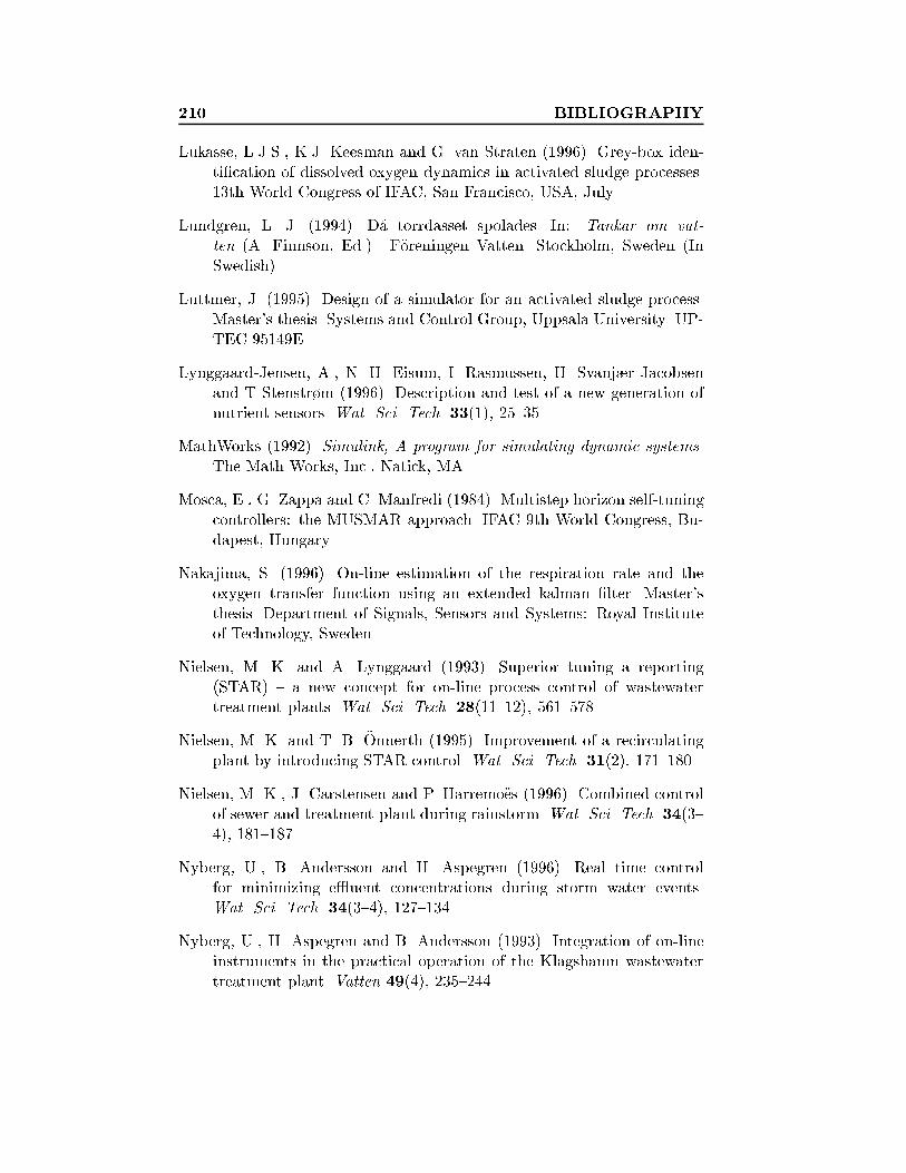
210 BIBLIOGRAPHY
Lukasse, L.J.S., K.J. Keesman and G. van Straten (1996). Grey-box iden-ti�cation of dissolved oxygen dynamics in activated sludge processes.13th World Congress of IFAC, San Francisco, USA, July.
Lundgren, L. J. (1994). D�a torrdasset spolades. In: Tankar om vat-
ten (A. Finnson, Ed.). F�oreningen Vatten. Stockholm, Sweden (InSwedish).
Luttmer, J. (1995). Design of a simulator for an activated sludge process.Master's thesis. Systems and Control Group, Uppsala University. UP-TEC 95149E.
Lynggaard-Jensen, A., N. H. Eisum, I. Rasmussen, H. Svanj�r Jacobsenand T Stenstr�m (1996). Description and test of a new generation ofnutrient sensors. Wat. Sci. Tech. 33(1), 25{35.
MathWorks (1992). Simulink, A program for simulating dynamic systems.The Math Works, Inc., Natick, MA.
Mosca, E., G. Zappa and C. Manfredi (1984). Multistep horizon self-tuningcontrollers: the MUSMAR approach. IFAC 9th World Congress, Bu-dapest, Hungary.
Nakajima, S. (1996). On-line estimation of the respiration rate and theoxygen transfer function using an extended kalman �lter. Master'sthesis. Department of Signals, Sensors and Systems: Royal Instituteof Technology, Sweden.
Nielsen, M. K. and A. Lynggaard (1993). Superior tuning a reporting(STAR) { a new concept for on-line process control of wastewatertreatment plants. Wat. Sci. Tech. 28(11{12), 561{578.
Nielsen, M. K. and T. B. �Onnerth (1995). Improvement of a recirculatingplant by introducing STAR control. Wat. Sci. Tech. 31(2), 171{180.
Nielsen, M. K., J. Carstensen and P. Harremo�es (1996). Combined controlof sewer and treatment plant during rainstorm. Wat. Sci. Tech. 34(3{4), 181{187.
Nyberg, U., B. Andersson and H. Aspegren (1996). Real time controlfor minimizing e�uent concentrations during storm water events.Wat. Sci. Tech. 34(3{4), 127{134.
Nyberg, U., H. Aspegren and B. Andersson (1993). Integration of on-lineinstruments in the practical operation of the Klagshamn wastewatertreatment plant. Vatten 49(4), 235{244.
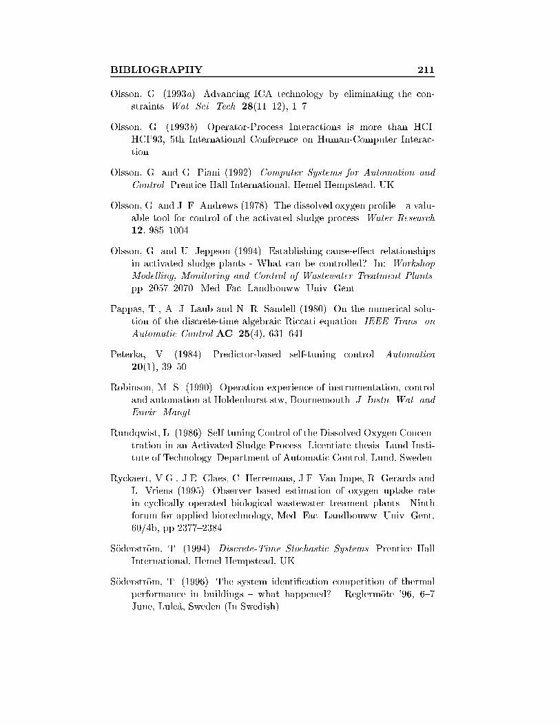
BIBLIOGRAPHY 211
Olsson, G. (1993a). Advancing ICA technology by eliminating the con-straints. Wat. Sci. Tech. 28(11{12), 1{7.
Olsson, G. (1993b). Operator-Process Interactions is more than HCI.HCI'93, 5th International Conference on Human-Computer Interac-tion.
Olsson, G. and G. Piani (1992). Computer Systems for Automation and
Control. Prentice Hall International, Hemel Hempstead, UK.
Olsson, G. and J. F. Andrews (1978). The dissolved oxygen pro�le { a valu-able tool for control of the activated sludge process. Water Research
12, 985{1004.
Olsson, G. and U. Jeppson (1994). Establishing cause-e�ect relationshipsin activated sludge plants - What can be controlled?. In: WorkshopModelling, Monitoring and Control of Wastewater Treatment Plants.pp. 2057{2070. Med. Fac. Landbouww. Univ. Gent.
Pappas, T., A. J. Laub and N. R. Sandell (1980). On the numerical solu-tion of the discrete-time algebraic Riccati equation. IEEE Trans. on
Automatic Control AC{25(4), 631{641.
Peterka, V. (1984). Predictor-based self-tuning control. Automatica
20(1), 39{50.
Robinson, M. S. (1990). Operation experience of instrumentation, controland automation at Holdenhurst stw, Bournemouth. J. Instn. Wat. and
Envir. Mangt.
Rundqwist, L. (1986). Self-tuning Control of the Dissolved Oxygen Concen-tration in an Activated Sludge Process. Licentiate thesis. Lund Insti-tute of Technology. Department of Automatic Control, Lund, Sweden.
Ryckaert, V.G., J.E. Claes, C. Herremans, J.F. Van Impe, R. Gerards andL. Vriens (1995). Observer based estimation of oxygen uptake ratein cyclically operated biological wastewater treament plants. Ninthforum for applied biotechnology, Med. Fac. Landbouww. Univ. Gent,60/4b, pp 2377{2384.
S�oderstr�om, T. (1994). Discrete-Time Stochastic Systems. Prentice HallInternational, Hemel Hempstead, UK.
S�oderstr�om, T. (1996). The system identi�cation competition of thermalperformance in buildings { what happened? Reglerm�ote '96, 6{7June, Lule�a, Sweden (In Swedish).
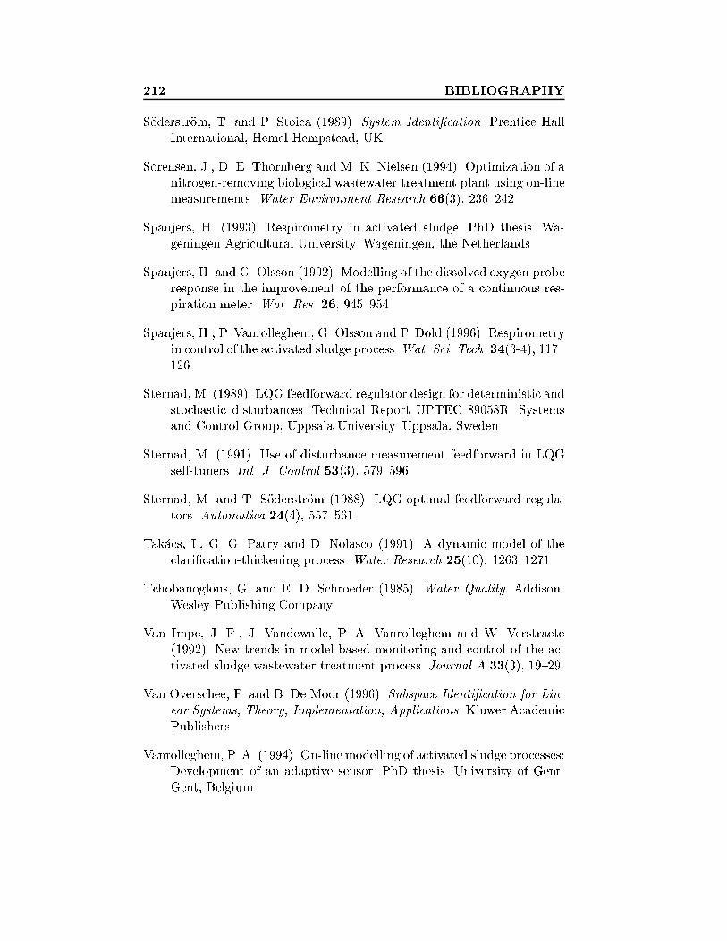
212 BIBLIOGRAPHY
S�oderstr�om, T. and P. Stoica (1989). System Identi�cation. Prentice HallInternational, Hemel Hempstead, UK.
Sorensen, J., D. E. Thornberg and M. K. Nielsen (1994). Optimization of anitrogen-removing biological wastewater treatment plant using on-linemeasurements. Water Environment Research 66(3), 236{242.
Spanjers, H. (1993). Respirometry in activated sludge. PhD thesis. Wa-geningen Agricultural University. Wageningen, the Netherlands.
Spanjers, H. and G. Olsson (1992). Modelling of the dissolved oxygen proberesponse in the improvement of the performance of a continuous res-piration meter. Wat. Res. 26, 945{954.
Spanjers, H., P. Vanrolleghem, G. Olsson and P. Dold (1996). Respirometryin control of the activated sludge process.Wat. Sci. Tech. 34(3-4), 117{126.
Sternad, M. (1989). LQG feedforward regulator design for deterministic andstochastic disturbances. Technical Report UPTEC 89058R. Systemsand Control Group, Uppsala University. Uppsala, Sweden.
Sternad, M. (1991). Use of disturbance measurement feedforward in LQGself-tuners. Int. J. Control 53(3), 579{596.
Sternad, M. and T. S�oderstr�om (1988). LQG-optimal feedforward regula-tors. Automatica 24(4), 557{561.
Tak�acs, I., G. G. Patry and D. Nolasco (1991). A dynamic model of theclari�cation-thickening process. Water Research 25(10), 1263{1271.
Tchobanoglous, G. and E. D. Schroeder (1985). Water Quality. Addison-Wesley Publishing Company.
Van Impe, J. F., J. Vandewalle, P. A. Vanrolleghem and W. Verstraete(1992). New trends in model-based monitoring and control of the ac-tivated sludge wastewater treatment process. Journal A 33(3), 19{29.
Van Overschee, P. and B. De Moor (1996). Subspace Identi�cation for Lin-
ear Systems, Theory, Implementation, Applications. Kluwer AcademicPublishers.
Vanrolleghem, P. A. (1994). On-line modelling of activated sludge processes:Development of an adaptive sensor. PhD thesis. University of Gent.Gent, Belgium.
BIBLIOGRAPHY 213
Vanrolleghem, P. A. and W. Verstraete (1993). On-line monitoring equip-ment for wastewater treatment processes: State of the art. In: Pro-
ceedings TI-KVIV Studiedag Optimalisatie van Waterzuiveringsinstal-
laties door Proceskontrole en -sturing. Gent, Belgium.
Vanrolleghem, P. A., L. K. Vermeersch, D. Dochain and G. C. Vansteenkiste(1993). Modelling of a nonlinear distributed parameter bioreactor: Op-timisation of a nutrient removal process. In: Modelling and Simulation
(A. Pav�e, Ed.). pp. 563{567. SCS, San Diego.
Vanrolleghem, P. A., U. Jeppsson, J. Carstensen, B. Carlsson and G. Olsson(1996). Integration of wastewater treatment plant design and operation{ A systematic approach using cost functions.. Wat. Sci. Tech. 34(3{4), 159{171.
Viberg, M. (1994). Subspace methods in system identi�cation. In: Proceed-ings IFAC SYSID '94. Copenhagen, Denmark.
Viberg, M., B. Wahlberg and B. Ottersten (1995). Anaysis of State SpaceSystem Identi�cation methods based on instrumental variables andsubspace �tting. Technical Report CTH-TE-34. Dept. of Applied Elec-tronics, Chalmers University of Technology, Sweden.
Wagner, M. and H. J. P�opel (1996). Surface active agents and their in u-ence on oxygen transfer. Wat. Sci. Tech. 34(3{4), 249{256.
Wells, C. H. (1979). Computer control of fully nitrifying activated sludgeprocesses. Instrumentation Technology 4, 32{36.
Wikstr�om, A. (1993). Simnon models for activated sludge systems. Techni-cal report. Dept. of Industrial Electrical Eng. and Automation, LundInstitute of Technology.
Wikstr�om, A. (1994). Simulink models for activated sludge systems. Tech-nical report. Dept. of Industrial Electrical Eng. and Automation, LundInstitute of Technology.
Youssef, C. B., G. Roux and B. Dahhou (1995). Multivariable adaptivepredictive control of nonlinear systems: Application to a multistagewastewater treatment process. In: Proc. of 3rd European Control Con-
ference. pp. 3585{3590. Rome, Italy.
Yuan, Z., H. Bogaert, P. Vanrolleghem, C. Thoeye, G. Vansteenkiste andW. Verstraete (1996). Carbon dosage control for predenitri�cation pro-cesses. In: Proceedings Workshop Modelling, Monitoring and Control

214 BIBLIOGRAPHY
of Wastewater Treatment Plants. pp. 1733{1743. Med. Fac. Land-bouww. Univ. Gent, 61/4a.


