Page 1
OFDM PAPR REDUCTION WITH LINEAR CODING
AND CODEWORD MODIFICATION
A THESIS SUBMITTED TO
THE GRADUATE SCHOOL OF NATURAL AND APPLIED SCIENCES
OF
MIDDLE EAST TECHNICAL UNIVERSITY
BY
AYL�N SUSAR
IN PARTIAL FULFILLMENT OF THE REQUIREMENTS
FOR THE DEGREE OF MASTER OF SCIENCE
IN ELECTRICAL AND ELECTRONICS ENGINEERING
AUGUST 2005
Page 2
Approval of the Graduate School of Natural and Applied Sciences
Prof. Dr. Canan ÖZGEN
Director I certify that this thesis satisfies all the requirements as a thesis for the degree of Master of Science.
Prof. Dr. �smet ERKMEN Head of Department
This is to certify that we have read this thesis and that in our opinion it is fully adequate, in scope and quality, as a thesis for the degree of Master of Science.
Prof. Dr. Yalçın TANIK Supervisor Examining Committee Members Prof. Dr. Mete SEVERCAN (METU,EE)
Prof. Dr. Yalçın TANIK (METU,EE)
Prof. Dr. Rüyal ERGÜL (METU,EE)
Assoc. Prof. Dr. Melek YÜCEL (METU,EE)
Adil BAKTIR (ASELSAN)
Page 3
iii
I hereby declare that all information in this document has been obtained and presented in accordance with academic rules and ethical conduct. I also declare that, as required by these rules and conduct, I have fully cited and referenced all material and results that are not original to this work. Name, Last name : Aylin SUSAR
Signature :
Page 4
iv
ABSTRACT
OFDM PAPR REDUCTION WITH LINEAR CODING
AND CODEWORD MODIFICATION
SUSAR, Aylin
M.Sc., Department of Electrical and Electronics Engineering
Supervisor: Prof. Dr. Yalçın TANIK
August 2005, 116 pages
In this thesis, reduction of the Peak-to-Average Power Ratio (PAPR) of
Orthogonal Frequency Division Multiplexing (OFDM) is studied. A new PAPR
reduction method is proposed that is based on block coding the input data and
modifying the codeword until the PAPR is reduced below a certain threshold. The
method makes use of the error correction capability of the block code employed.
The performance of the algorithm has been investigated through theoretical
models and computer simulations. For performance evaluation, a new gain
parameter is defined. The gain parameter considers the SNR loss caused by
modification of the codeword together with the PAPR reduction achieved. The
gain parameter is used to compare a plain OFDM system with the system
employing the PAPR reduction algorithm. The algorithm performance is
examined through computer simulations and it is found that power reductions
around 2-3 dB are obtained especially for low to moderate number of channels and
relatively strong codes.
Keywords: OFDM, PAPR, block code, SNR
Page 5
v
ÖZ
DO�RUSAL KODLAMA VE KODLANMI� VER� DE���T�R�LMES�
YÖNTEM�YLE OFDM �Ç�N TEPE GÜÇ/ORTALAMA GÜÇ ORANI
AZALTIMI
SUSAR, Aylin
Yüksek Lisans, Elektrik ve Elektronik Mühendisli�i Bölümü
Tez Yöneticisi: Prof. Dr. Yalçın TANIK
A�ustos 2005, 116 sayfa
Bu tezde, Dikgen Sıklık Bölümlü Ço�ullama (OFDM) yönteminde Tepe
Güç/Ortalama Güç Oranı (PAPR) dü�ürülmesi üzerine çalı�ılmı�tır. Giri� verisinin
blok kodlanması ve kodlanmı� verinin PAPR’ı belirli bir e�ik seviyesinin altına
dü�ene kadar de�i�tirilmesi temeline dayanan yeni bir PAPR azaltım metodu
önerilmi�tir. Metod, uygulanan blok kodun hata düzeltme yetene�inden faydalanır.
Algoritmanın performansı teorik modeller ve bilgisayar benzetimleri aracılı�ıyla
incelenmi�tir. Performans de�erlendirmesi için yeni bir kazanç parametresi
tanımlanmı�tır. Kazanç parametresi, kodlanmı� verinin modifikasyonundan
kaynaklanan SNR kaybı ile birlikte ba�arılan PAPR azaltımını da dikkate alır.
Kazanç parametresi, basit OFDM sistemi ile PAPR dü�ürme algoritmasını
kullanan sistemi kar�ıla�tırmak için kullanılmı�tır. Algoritmanın performansı
bilgisayar benzetimleri ile incelenmi�tir ve ortalama kanal sayıları ile nispeten
güçlü kodlar için 2-3 dB civarında güç azaltımının elde edildi�i bulunmu�tur.
Page 6
vi
Anahtar Kelimeler: Dikgen Sıklık Bölümlü Ço�ullama (OFDM), Tepe
Güç/Ortalama Güç Oranı (PAPR), blok kod, Sinyal-Gürültü Oranı (SNR)
Page 8
viii
ACKNOWLEDGEMENTS I would like to thank to Prof. Dr. Yalçın Tanık for his valuable guidance and
helpful suggestions during the development and improvement stages of this thesis.
I am grateful to Adil Baktır for his tolerance throughout this study.
Thanks a lot to my parents for their constant support and encouragement which
made my research easier.
Special thanks to my sister Ayça and little brother Anıl for spending great effort to
increase my motivation and morale.
I would like to give my special appreciation to Evrim Onur Arı for sharing his
invaluable experiences of MATLAB and especially for his endless love which was
the motivation behind long hours of study.
Page 9
ix
TABLE OF CONTENTS PLAGIARISM.........................................................................................................iii
ABSTRACT…………………………………….………………………………...iv ÖZ…………………………………………………………………………………v ACKNOWLEDGEMENTS……....……………………………………………..viii TABLE OF CONTENTS…………………………………………………………ix LIST OF TABLES.................................................................................................xii LIST OF FIGURES..............................................................................................xiii LIST OF ABBREVIATIONS………………………………………………...….xv CHAPTER
1. INTRODUCTION………………………………………………………….… 1
2. OVERVIEW OF OFDM…...…………………………………………...………6
2.1.General Structure of OFDM………………………………………...……..6
2.2.Basic Techniques in OFDM……………………………………………...10
2.2.1. Windowing...……………………………………………….........10
2.2.2. Guard Time and Cyclic Prefix………...…………………………12
2.2.3. Synchronization…………………………………...……………..19
2.2.3.1. Sensitivity to Phase Noise……………...……………...19
2.2.3.2. Sensitivity to Frequency Offset………………………..20
2.2.3.3. Sensitivity to Timing Errors…………………………...21
2.2.3.4. Synchronization Techniques………………………… 21
2.2.3.4.1. Synchronization Using Cyclic Extension…21
2.2.3.4.2. Synchronization Using Special Training Symbols..………….………….....................22
Page 10
x
2.2.4. Bit loading.....................................................................................23
2.2.5. Peak-to-Average Power Ratio (PAPR)…………………………..24
2.3. Applications of OFDM……………………………………………...…...24
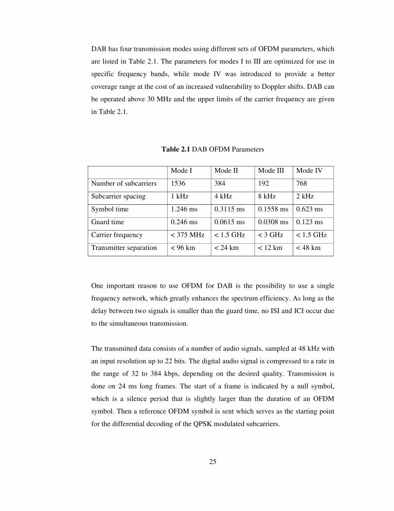
2.3.1. Digital Audio Broadcasting (DAB)……………………………...24
2.3.2. Terrestrial Digital Video Broadcasting…………………………..26
2.3.3. Magic WAND……………………………………………………27
2.3.4. IEEE 802.11, HYPERLAN/2 and MMAC Wireless LAN Standards.………………………………………………...29
3. PAPR REDUCTION TECHNIQUES………………...……………………….33
3.1. Introduction………………………………………...…………………….33
3.2. Clipping and Peak Windowing…………………………………………..34
3.3. Peak Cancellation………………………………………………………..35
3.4. Scrambling Techniques………………………………………………….38
3.4.1. Selected Mapping………………………………………………..39
3.4.2. Partial Transmit Sequences………………………………………41
3.5. Coding……………………………………………………………………43
4. PAPR REDUCTION WITH LINEAR CODING AND CODEWORD MODIFICATION……………………………………………….……………..46
4.1. Introduction……………………………………………………...……….46
4.2. Description of the Method……………………………………………….47
4.3. Fundamental Simulation Parameters…………………………………….56
4.3.1. Index-to-Change ………………………………………………...56
4.3.2. Rotation Direction……………………………………………….56
4.3.3. PAPR…………………………………………………………….58
4.4. Simulation Results of PAPR Reduction…………………………………64
5. PERFORMANCE OF THE CODING BASED PAPR REDUCTION
ALGORITHM …………………………………………………………………67
5.1. General Comparison Criteria…………………………………………….68
5.2. Coded OFDM Operation………………………………………………...68
5.3. PDF (Probability Density Function) of Instantaneous Power of OFDM Signal……………………………………………………………………72
Page 11
xi
5.4. Bit Error Probability, Block Error Probability and SNR Loss Relations for
Sys1……………………………………………………………………..74 5.5. Choosing Transmitter Threshold for Sys1…………………………...…..77
5.6. Bit Error Probability, Block Error Probability and SNR Loss Relations for Sys2………………………………………………………………...….....79
5.7. Choosing Transmitter Threshold for Sys2……………………………….83
5.8. Gain Definition Used for Performance Comparison…………………….86
5.9. Summary…………………………………………………………………90
6. NUMERICAL RESULTS……………………………………………………..92
6.1. Basic System Behaviour…………………………………………………92
6.2. Tables of Gain Parameters……………………………………………….99
6.2.1. Number of Channels…………………………………………...100
6.2.2. Clipping Rate…………………………………………………..101
6.2.3. Information Bit Rate…………………………………………...101
6.2.4. Code Rate………………………………………………………102
6.2.5. Code Length……………………………………………………103
7. SUMMARY AND CONCLUSIONS………………………………………...108
REFERENCES………………………………………………………………….111
APPENDIX A- GENERATOR POLYNOMIALS OF THE BCH CODES……115
Page 12
xii
LIST OF TABLES Table 2.1 DAB OFDM Parameters………………………………………………25
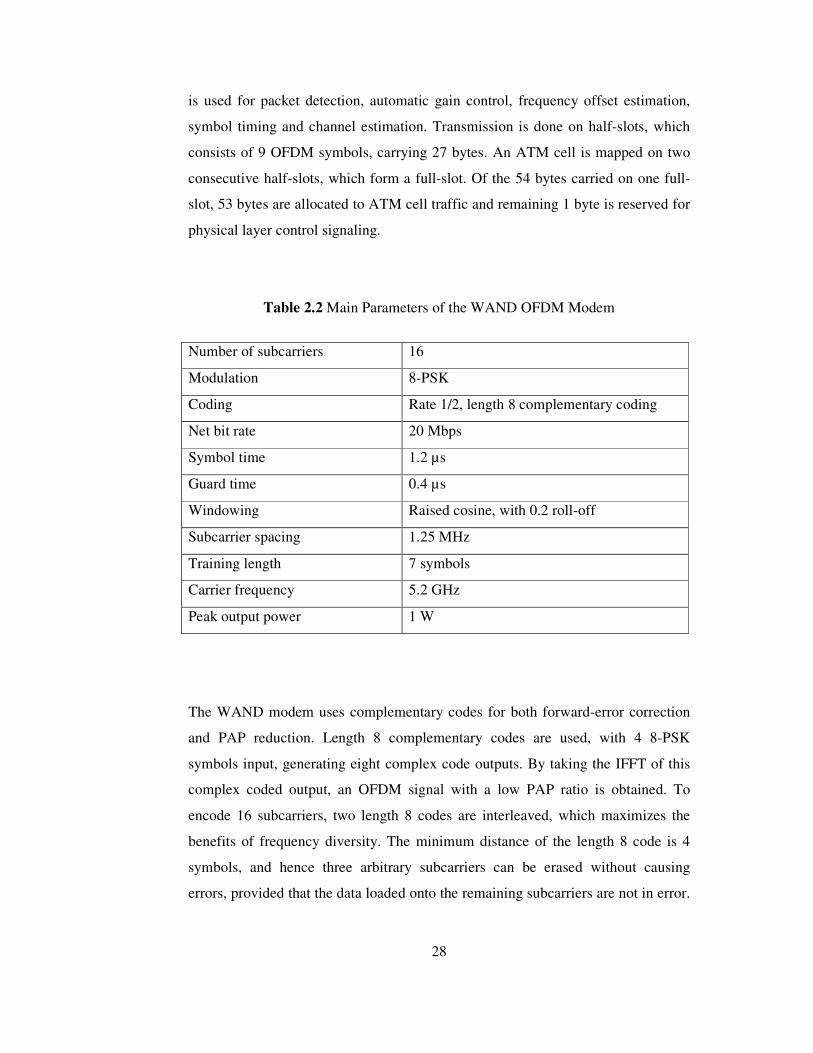
Table 2.2 Main Parameters of the WAND OFDM Modem……………………...28
Table 2.3 Main Parameters of the OFDM physical layer standards (IEEE 802.11a,
ETSI HYPERLAN type II and MMAC)………………………………32
Table 6.1 Gain Parameter for 32-Channels, Clipping Rate of One-per-Day and
Information Bit Rate of 100 Mbits/sec……………………………….104
Table 6.2 Gain Parameter for 32-Channels, Clipping Rate of One-per-Day and
Information Bit Rate of 8Mbits/sec…………………………………..104
Table 6.3 Gain Parameter for 128-Channels, Clipping Rate of One-per-Day and
Information Bit Rate of 100 Mbits/sec……………………………….105
Table 6.4 Gain Parameter for 32-Channels, Clipping Rate of One-per-Month and
Information Bit Rate of 100 Mbits/sec……………………………….105
Table 6.5 Gain Parameter for 32-Channels, Clipping Rate of One-per-Month and
Information Bit Rate of 8 Mbits/sec………………………………….106
Table 6.6 Gain Parameter for 128-Channels, Clipping Rate of One-per-Month and
Information Bit Rate of 100 Mbits/sec……………………………….106
Page 13
xiii
LIST OF FIGURES Figure 2.1 Block Diagram of an OFDM Transmitter……………………………...9
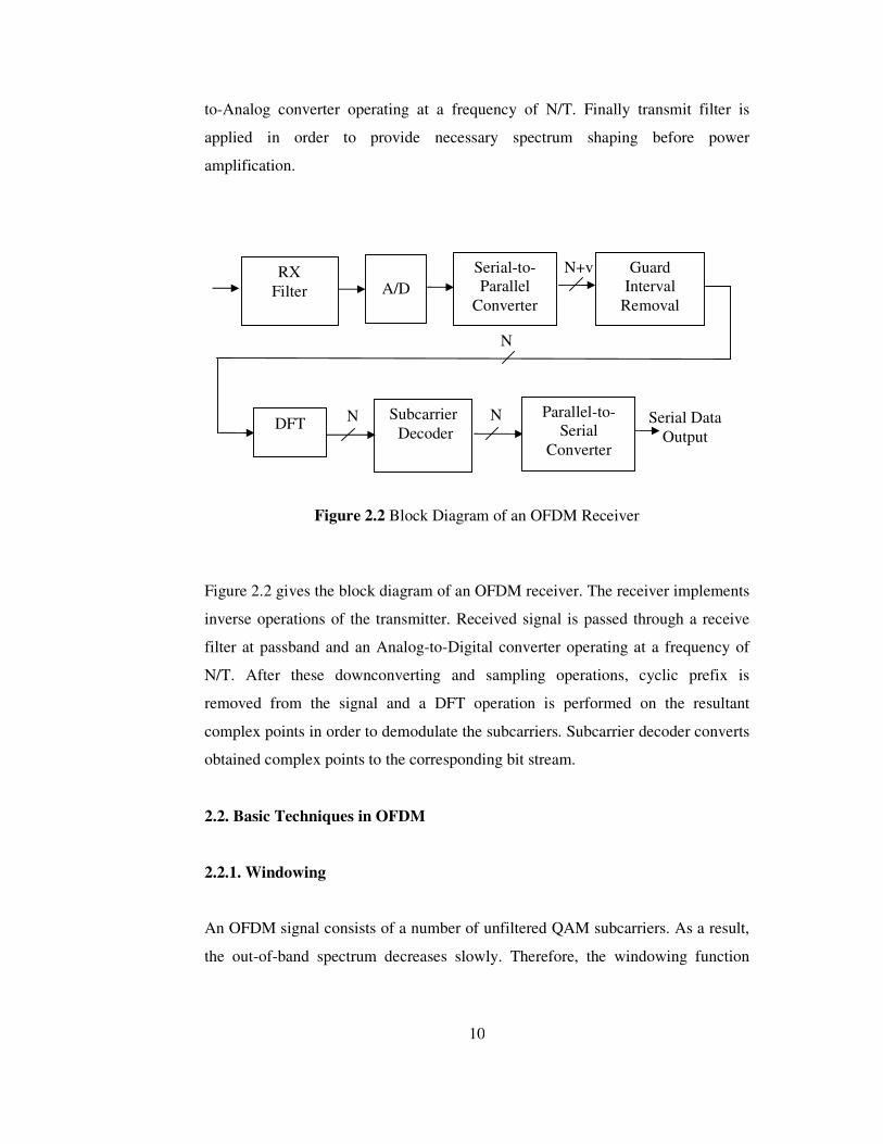
Figure 2.2 Block Diagram of an OFDM Receiver……………………………….10
Figure 2.3 Insertion of Guard Interval……………………………………………15
Figure 2.4 Insertion of Cyclic Prefix …………………………………………….16
Figure 2.5 Synchronization Using Cyclic Prefix…………………………………22
Figure 2.6 Synchronization Using Special Training Symbols……………………23
Figure 3.1 Clipping of OFDM Signal…………………………………………….34
Figure 3.2 Peak Windowing of OFDM Signal…………………………………...35
Figure 3.3 OFDM Transmitter with Peak Cancellation…………………………..37
Figure 3.4 Peak Cancellation Using FFT/IFFT to Generate Cancellation Signal..38
Figure 3.5 Block Diagram of Selected Mapping Method………………………...39
Figure 3.6 Subblock Configuration for Partial Transmit Sequences Method……42
Figure 3.7 Block Diagram of Partial Transmit Sequences Method………………43
Figure 4.1 System Block Diagram………………………………………………..47
Figure 4.2 Encoder & Mapper Block Diagram…………………………………..48
Figure 4.3 Encoder & Mapper Output for Single Coded Block…………………49
Figure 4.4 QPSK Bit Assignments………………………………………………49
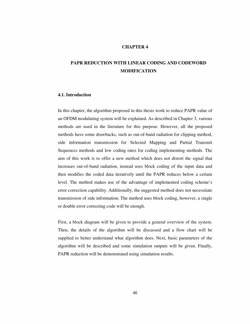
Figure 4.5 QPSK Modification for PAPR Reduction……………………………51
Figure 4.6 Amplitude Reduction of y[1]…………………………………………52
Figure 4.7 Algorithm Flow Chart 1/2..…………………………………………...53
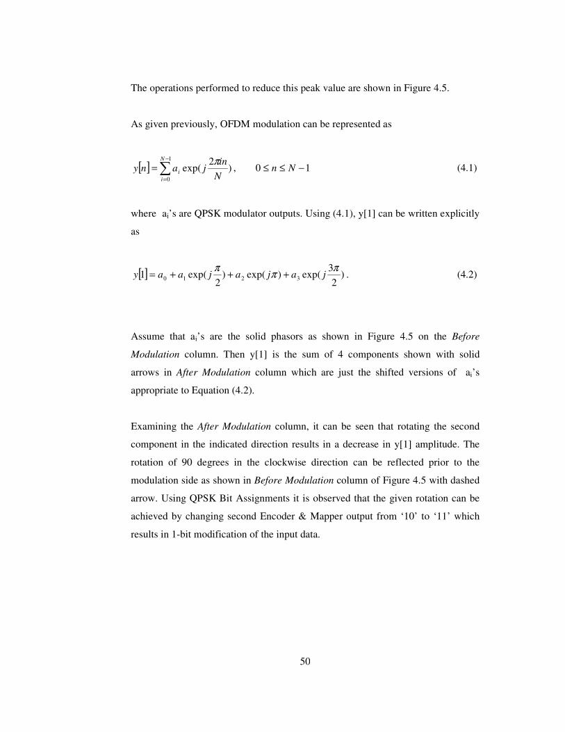
Figure 4.8 Algorithm Flow Chart 2/2…………………………………………….54
Figure 4.9 PAPR (in dB) of an OFDM System without Algorithm
Implementation……………………………………………………….60
Figure 4.10 PAPR (in dB) of an OFDM System with Algorithm
Implementation………………………………………………………61
Page 14
xiv
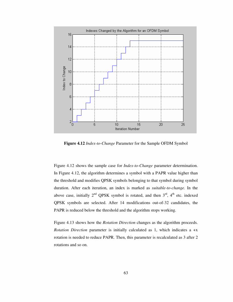
Figure 4.11 Step-by-Step PAPR Reduction During Algorithm
Implementation………………………………………………………62
Figure 4.12 Index-to-Change Parameter for the Sample OFDM Symbol………..63
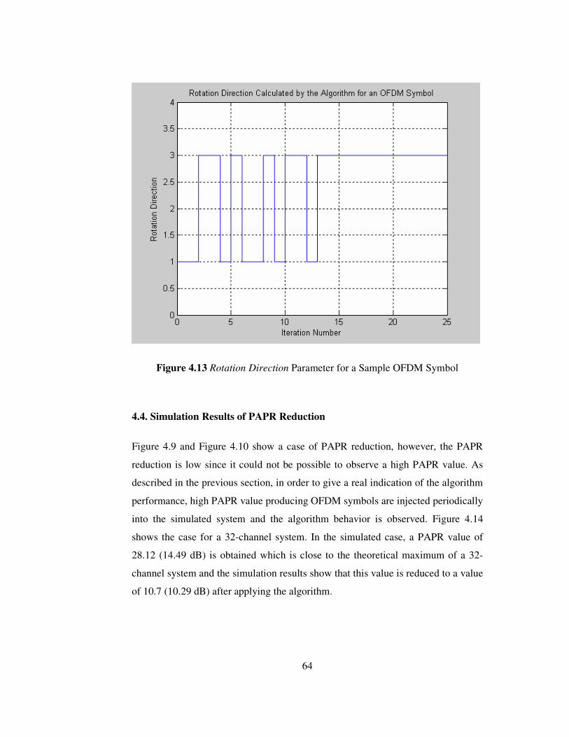
Figure 4.13 Rotation Direction Parameter for a Sample OFDM Symbol………..64
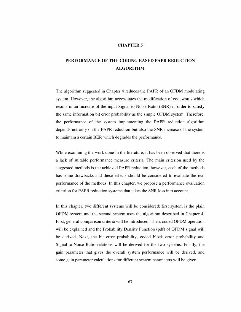
Figure 4.14 PAPR Reduction for 32-Channel OFDM System…………………...65
Figure 4.15 PAPR Reduction for 128-Channel OFDM System………………….66
Figure 5.1 Block Diagram of the Sample OFDM Transmitter…………………...69
Figure 5.2 OFDM Transmitter Input Block………………………………………69
Figure 5.3 Construction of N PreCode Blocks…………………...........................70
Figure 5.4 Construction of N Coded Blocks……………………………………..71
Figure 5.5 Block Diagram of the Sample OFDM Receiver……………………...71
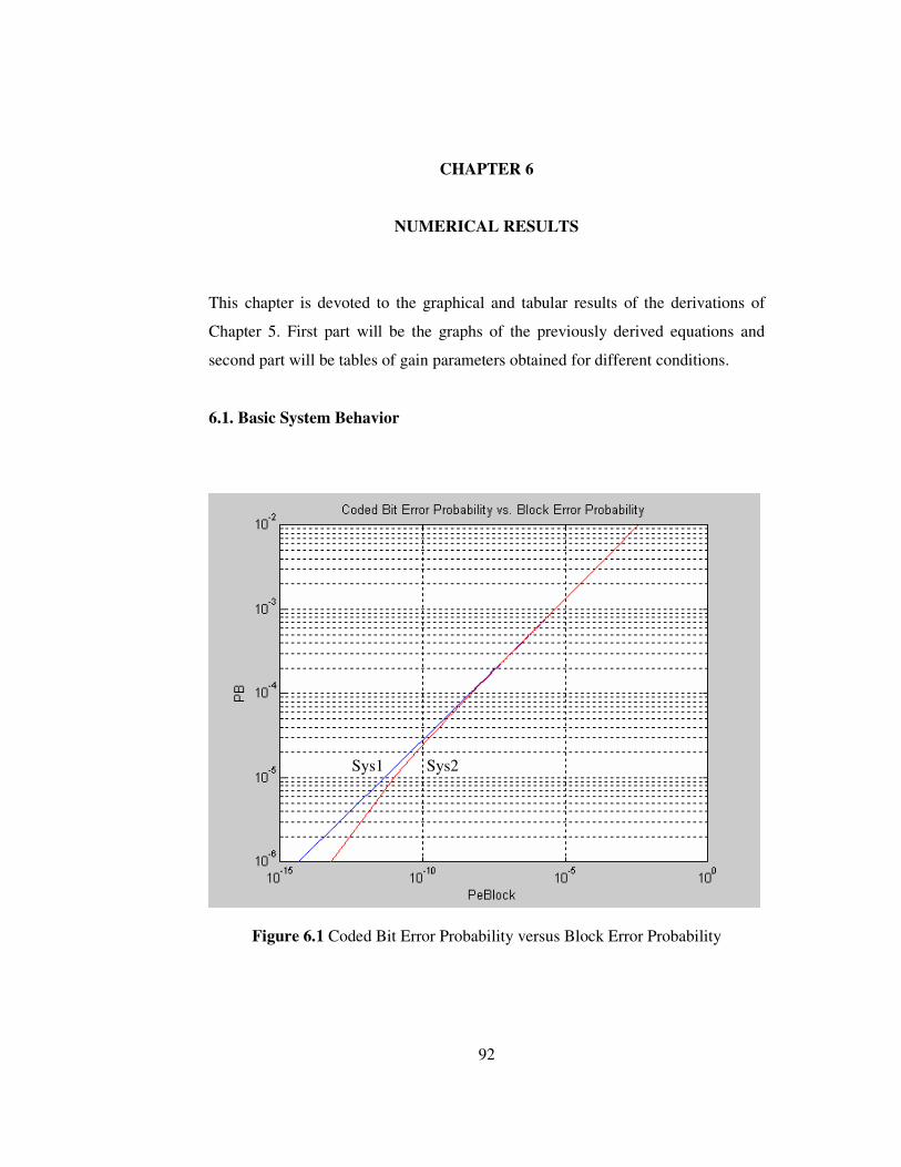
Figure 6.1 Coded Bit Error Probability versus Block Error Probability…..……..92
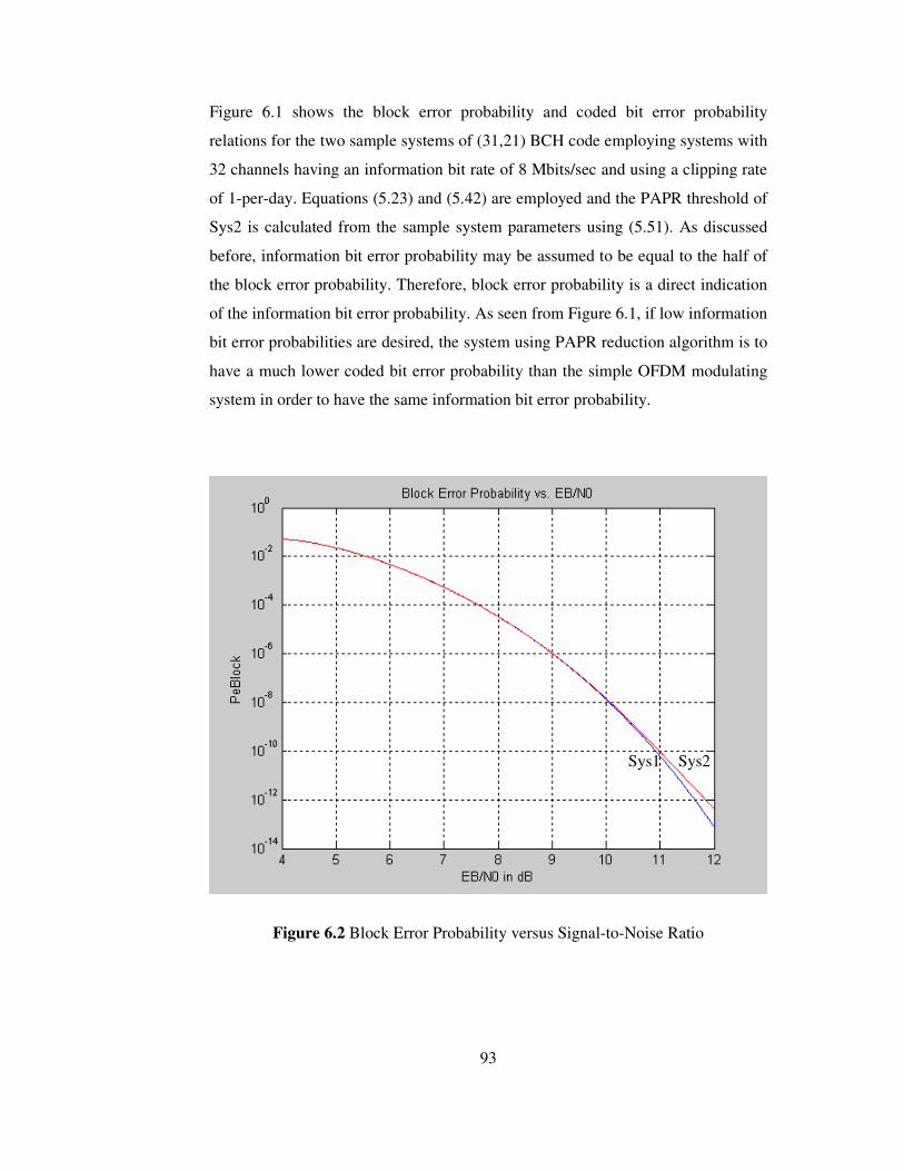
Figure 6.2 Block Error Probability versus Signal-to-Noise Ratio………………..93
Figure 6.3 Signal-to-Noise Ratio Loss versus Algorithm Threshold…………….94
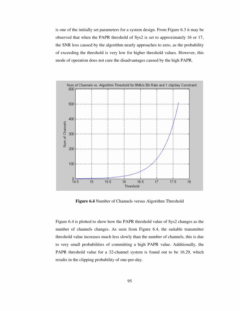
Figure 6.4 Number of Channels versus Algorithm Threshold…………………...95
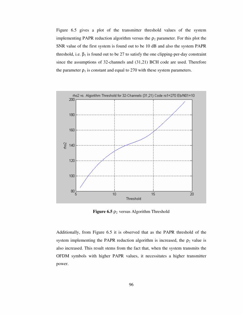
Figure 6.5 ρ2 versus Algorithm Threshold………..……………………………...96
Figure 6.6 Gain Parameter Ratio versus Algorithm Threshold……………...…...97
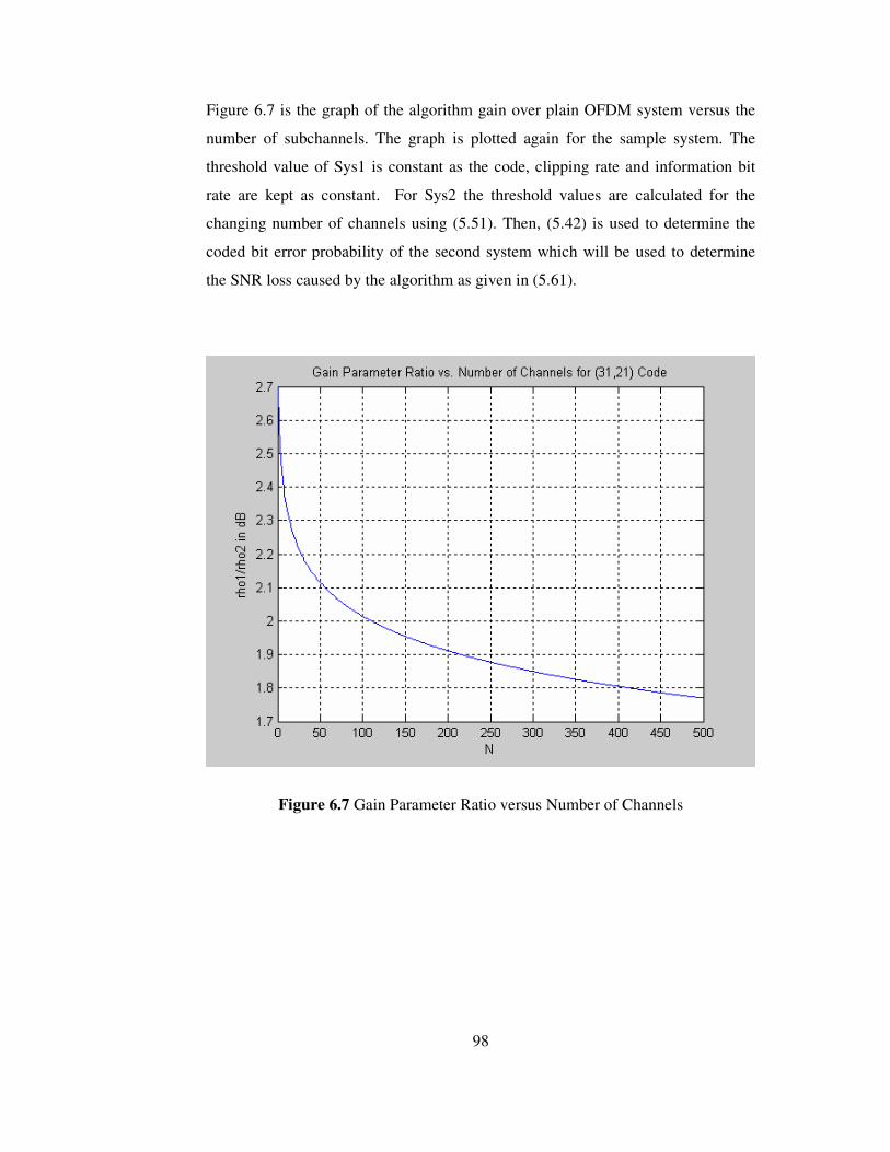
Figure 6.7 Gain Parameter Ratio versus Number of Channels…………………...98
Page 15
xv
LIST OF ABBREVIATIONS
MCM Multicarrier Modulation
OFDM Orthogonal Frequency Division Multiplexing
SNR Signal-to-Noise Ratio
ICI Intercarrier Interference
ISI Intersymbol Interference
FFT Fast Fourier Transform
IFFT Inverse Fast Fourier Transform
DFT Discrete Fourier Transform
IDFT Inverse Discrete Fourier Transform
PAPR Peak-to-Average Power Ratio
DAB Digital Audio Broadcasting
DVB Digital Video Broadcasting
EHF Extremely High Frequency
BER Bit Error Rate
SLM Selected Mapping
PTS Partial Transmit Sequences
pdf Probability Density Function
Page 16
1
CHAPTER 1
INTRODUCTION
Multicarrier Modulation (MCM) is the principle of transmitting data by dividing
the input data stream into several lower rate parallel bit streams and using these
substreams to modulate several carriers. The first systems using MCM were
military HF radio links in 1960s. In a classical MCM system, the total signal
frequency band is divided into N nonoverlapping frequency subchannels. Each
subchannel is modulated with a separate symbol and then the N subchannels are
frequency multiplexed. Spectral overlap of channels is avoided to eliminate
interchannel interference. However, this leads to inefficient use of the available
spectrum. To cope with the inefficiency, the ideas proposed from the 1960s were to
use MCM and Frequency Division Multiplexing (FDM) with overlapping
subchannels. Orthogonal Frequency Division Multiplexing (OFDM) is a special
case of multicarrier transmission. The word orthogonal indicates that there is a
mathematical relationship between the frequencies of carriers in the system. In a
normal MCM system, many carriers are spaced apart in such a way that the signals
can be received using conventional filters and demodulators. In such receivers,
guard bands are introduced between different carriers and in frequency domain
which results in reduction of spectrum efficiency. In OFDM, the carriers are
arranged such that the frequency spectrum of the individual carriers overlap and
the signals are still received without adjacent carrier interference. In order to
achieve this, the carriers are chosen to be mathematically orthogonal. The receiver
acts as a bank of demodulators, translating each carrier down to DC and integrating
the resulting signal over a symbol period to obtain raw data. In 1971, Weinstein
and Ebert [3] showed that OFDM waveforms can be generated using a Discrete
Fourier Transform (DFT) at the transmitter and receiver for the modulation and
demodulation.
Page 17
2
For a long time, usage of OFDM in practical systems was limited. Main reasons for
this limitation were the complexity of real time Fourier Transform and the linearity
required in RF power amplifiers. However since 1990s, OFDM is used for
wideband data communications over mobile radio FM channels, High-bit-rate
Digital Subscriber Lines (HDSL, 1.6Mbps), Asymmetric Digital Subscriber Lines
(ADSL, up to 6Mbps), Very-high-speed Digital Subscriber Lines (VDSL,
100Mbps), Digital Audio Broadcasting (DAB), and High Definition Television
(HDTV) terrestrial broadcasting.
OFDM has many advantages over single carrier systems. The implementation
complexity of OFDM is significantly lower than that of a single carrier system
with equalizer. When the transmission bandwidth exceeds coherence bandwidth of
the channel, resultant distortion may cause intersymbol interference (ISI). Single
carrier systems solve this problem by using a linear or nonlinear equalization. The
problem with this approach is the complexity of effective equalization algorithms.
OFDM systems divide available channel bandwidth into a number of subchannels.
By selecting the subchannel bandwidth smaller than the coherence bandwidth of
the frequency selective channel, the channel appears to be nearly flat and no
equalization is needed. Also by inserting a guard time at the beginning of OFDM
symbol during which the symbol is cyclically extended, intersymbol interference
(ISI) and intercarrier interference (ICI) can be completely eliminated, if the
duration of guard period is properly chosen. This property of OFDM makes the
single frequency networks possible. In single frequency networks, transmitters
simultaneously broadcast at the same frequency, which causes intersymbol
interference. Additionally, in relatively slow time varying channels, it is possible to
significantly enhance the capacity by adapting the data rate per subcarrier
according to the signal-to-noise ratio (SNR) of that particular subcarrier. Another
advantage of OFDM over single carrier systems is its robustness against
narrowband interference because such interference affects only a small percentage
of the subcarriers.
Page 18
3
Beyond all these advantages, OFDM has some drawbacks compared to single
carrier systems. Two of the problems with OFDM are the carrier phase noise and
frequency offset. Carrier phase noise is caused by imperfections in the transmitter
and receiver oscillators. Frequency offsets are created by differences between
oscillators in transmitter and receiver, Doppler shifts, or phase noise introduced by
nonlinear channels. There are two destructive effects caused by a carrier frequency
offset in an OFDM system. One is the reduction of signal amplitude since sinc (.)
functions are shifted and no longer sampled at the peak, and the other is the
introduction of ICI from the other carriers. The latter is caused by the loss of
orthogonality between the subchannels. Sensitivity to phase noise and frequency
offsets increases with the number of subcarriers and with the constellation size
used for subcarrier modulation. For single carrier systems, phase noise and
frequency offsets only give degradation in the receiver SNR, rather than
introducing ICI. That is why the sensitivity to frequency offsets and phase noise
are mentioned as disadvantages of OFDM relative to single carrier systems.
The most important disadvantage of OFDM systems is that highly linear RF
amplifiers are needed. An OFDM signal consists of a number of independently
modulated subcarriers, which can give a large Peak-to-Average Power Ratio
(PAPR) when added up coherently. When N signals are added with the same
phase, they produce a peak power that is N times the average power. In order to
avoid nonlinear distortion, highly linear amplifiers are required which cause a
severe reduction in power efficiency. Several methods are explained in the
literature in order to solve this problem.
Most widely used methods are clipping and peak windowing the OFDM signal
when a high PAPR is encountered. However these methods distort the original
OFDM signal resulting in an increase in the bit error probability. There are other
methods that do not distort the signal. Two of these methods can be listed as
Partial Transmit Sequences [5,6] and Selected Mapping [7,8]. The principle behind
these methods is to transmit the OFDM signal with the lowest PAPR value among
Page 19
4
a number of candidates all of which represent the same information. Coding is
another commonly used method. In this case the information bits are coded in a
way that no high peaks are generated. Mainly Golay codes, Reed Muller codes and
linear block codes are used [9,10,11,12].
In this thesis a method based on coding is proposed to reduce the PAPR value of an
OFDM signal. The method uses linear block coding and the error correction
capability of the code. In the literature there are a number of similar methods
proposed to reduce the PAPR value. Their performance is evaluated according to
the final PAPR value achieved only. However, some of the methods result in an
increase in Bit Error Rate (BER) and some of the methods require transmission of
side information on a secure channel for the correct reception of the transmitted
data. These effects need to be considered for accurate performance calculations.
Hence, there is a deficiency in the performance evaluation criterion. This thesis
provides a means of performance evaluation of a PAPR reducing algorithm.
This thesis is organized as follows. Chapter 2 is a rather detailed overview of
OFDM. Main equations are derived and main techniques of OFDM such as
windowing, guard time & cyclic prefixing, synchronization, bit loading and PAPR
are explained. Afterwards, applications of OFDM are discussed.
Chapter 3 provides a deep insight into the PAPR problem by discussing the
methods used in the literature. Block diagram of each method is provided; their
advantages and disadvantages are discussed.
In Chapter 4, the PAPR reduction method suggested in the thesis is explained.
Detailed block diagrams and some MATLAB outputs are given to clarify how the
algorithm works.
Chapter 5 explains the second objective of the thesis: We suggest a method to
compare the algorithm implementing transmission system with a plain OFDM
Page 20
5
modulating system under a very low clipping rate condition. The SNR loss caused
by the algorithm is taken into account and the systems are compared for the case of
equal information bit error probabilities. Derivations of the performance
comparison equations are provided in this chapter.
Chapter 6 contains the graphs explaining system behavior. Additionally, this
chapter provides the numerical results obtained by algorithm implementation and
system comparison.
Finally, Chapter 7 includes some concluding remarks.
Page 21
6
CHAPTER 2
OVERVIEW OF OFDM
In this chapter, first the general structure of an OFDM system will be mentioned.
The second part will be about main techniques of OFDM. Finally, applications of
OFDM will be examined.
2.1. General Structure of OFDM
The basic principle of OFDM is to split a high rate input data stream into a number
of lower rate streams that are transmitted simultaneously over a number of
subcarriers. Because the transmission rate is slower in parallel subcarriers, a
frequency selective channel appears to be flat to each subcarrier. ISI is eliminated
almost completely by adding a guard interval at the beginning of each OFDM
symbol. However, instead of using an empty guard time, this interval is filled with
a cyclically extended version of the OFDM symbol. This method is used to avoid
ICI.
OFDM is a special case of Multicarrier Modulation (MCM). In MCM, input data
stream is divided into lower rate substreams, and these substreams are used to
modulate several subcarriers. In general, the spacing between these subcarriers is
large enough such that individual spectrum of subcarriers do not overlap. Therefore
the receiver uses a bandpass filter tuned to that subcarrier frequency in order to
demodulate the signal. In OFDM, subcarrier spacing is kept at minimum, while
still preserving the time domain orthogonality between subcarriers, even though
the individual frequency spectrum may overlap. The minimum subcarrier spacing
should equal to 1/T, where T is the symbol period.
Page 22
7
An OFDM symbol in baseband is defined as:
�−
−=+=
12/
2/2/ )()
2exp()(
N
NiNi ts
Tit
jatxπ
,0 Tt ≤≤ (2.1)
where, 2/Nia + denotes the complex symbol modulating the i-th carrier, s(t) is the
time window function defined in the interval [0,T], N is the number of subcarriers,
and T is the OFDM symbol period. Subcarriers are spaced �f=1/T apart. The
correlation coefficient between the subcarriers may be defined as:
� −=T
kn dtTnt
jTkt
jT 0
)2
exp()2
exp(1 ππρ (2.2)
As can be seen from (2.2),
��
���
≠
==
kn
knkn ,0
,1ρ (2.3)
Therefore, OFDM signal of the form (2.1) satisfies the condition of mutual
orthogonality between subcarriers in the symbol interval. In order to obtain the
data modulating the k-th subcarrier OFDM symbol should be downconverted with
a frequency of k/T, and then integrated over the symbol period [1]. We can assume
that s(t) is a rectangular window defined in [0,T] for simplicity. Then above
operation may be shown as:
Resultant signal= � �−
−=+−
T N
NiNi dt
Tit
jaTkt
jT 0
12/
2/2/ )
2exp()
2exp(
1 ππ
= �� −−
−=+
TN
NiNi dt
Tit
jTkt
jT
a0
12/
2/2/ )
2exp()
2exp(
1 ππ. (2.4)
Page 23
8
Using (2.3) and (2.4) together,
Resultant signal= 2/Nka + .
Considering the sequential transmission of symbols, the baseband signal at the
OFDM modulator output can be expressed as:
��−
−=+ −−=
12/
2/,2/ ),()
)(2exp()(
N
NinNi
n
nTtsT
nTtijatx
π (2.5)
where nNia ,2/+ represents the data modulating the i-th carrier of the n-th OFDM
symbol. The n-th OFDM symbol is transmitted in the time interval [nT, nT+T].
Assuming that the windowing function s(t) is nonzero only in [0,T] interval, if N
samples are taken from x(t) at time instants {nT+kT/N, k=0…N-1}, the result will
be [1]:
y[k]=x(nT+kT/N)
= ��−
−=+ −+−+12/
2/,2/ )/()
)/(2exp(
N
NinNi
n
nTNkTnTsT
nTNkTnTija
π
= �−
−=+
12/
2/,2/ ),/()
2exp(
N
NinNi NkTs
Nik
jaπ
0 � k � N-1. (2.6)
It can be seen from (2.6) that, N samples taken from n-th OFDM symbol at a rate
of N/T can be obtained by taking N-point inverse Discrete Fourier Transform
(IDFT) of the input data ak,n, k=0…N-1, weighted by the window function s(t) at
the sampling time instants.
Page 24
9
Figure 2.1 Block Diagram of an OFDM Transmitter
Figure 2.1 shows a basic OFDM transmitter structure. The serial input data stream
is divided into frames of Nf bits. These Nf bits are arranged into N groups, where
N is the number of subcarriers. The number of bits in each of the N groups
determines the constellation size for that particular subcarrier. For example, if all
the subcarriers are modulated by QPSK then each of the groups consists of 2 bits,
if 16-QAM modulation is used each group contains 4 bits. This scheme is called as
fixed loading. However, this is not the only way of distributing input bits among
the subchannels. Nf bits could be divided among subcarriers according to the
channel states. Therefore, one of the subcarriers can be modulated with 16-QAM
whereas another one can be modulated with 32-QAM, etc. In this case, the former
subcarrier consists of 4 bits and the latter subcarrier consists of 5 bits. This scheme
is named as adaptive loading. Hence, OFDM can be considered as N independent
QAM channels, each having a different QAM constellation but each operating at
the same symbol rate 1/T. After signal mapping, N complex points are obtained.
These complex points are passed through an IDFT block. Cyclic prefix of length v
is added to the IDFT output in order to combat with ICI and ISI. After Parallel–to-
Serial conversion, windowing function is applied. The output is fed into a Digital-
N+v
N
N N Serial Data Input
Serial-to-Parallel
Converter
Signal Mapper IDFT
Guard Interval Insertion
Parallel-to-Serial
Converter
Window &
D/A
TX Filter &
PA.
Page 25
10
to-Analog converter operating at a frequency of N/T. Finally transmit filter is
applied in order to provide necessary spectrum shaping before power
amplification.
Figure 2.2 Block Diagram of an OFDM Receiver
Figure 2.2 gives the block diagram of an OFDM receiver. The receiver implements
inverse operations of the transmitter. Received signal is passed through a receive
filter at passband and an Analog-to-Digital converter operating at a frequency of
N/T. After these downconverting and sampling operations, cyclic prefix is
removed from the signal and a DFT operation is performed on the resultant
complex points in order to demodulate the subcarriers. Subcarrier decoder converts
obtained complex points to the corresponding bit stream.
2.2. Basic Techniques in OFDM
2.2.1. Windowing
An OFDM signal consists of a number of unfiltered QAM subcarriers. As a result,
the out-of-band spectrum decreases slowly. Therefore, the windowing function
N+v
N
N N Serial Data Output
Serial-to-Parallel
Converter
Subcarrier Decoder DFT
Guard Interval
Removal
Parallel-to-Serial
Converter
A/D
RX Filter
Page 26
11
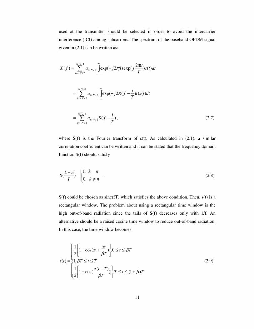
used at the transmitter should be selected in order to avoid the intercarrier
interference (ICI) among subcarriers. The spectrum of the baseband OFDM signal
given in (2.1) can be written as:
� �−
−=
∞
∞−+ −=
12/
2/2/ )()
2exp()2exp()(
N
NiNi dtts
Tit
jftjafXππ
� �−
−=
∞
∞−+ −−=
12/
2/2/ )())(2exp(
N
NiNi dttst
Ti
fja π
�−
−=+ −=
12/
2/2/ )(
N
NiNi T
ifSa , (2.7)
where S(f) is the Fourier transform of s(t). As calculated in (2.1), a similar
correlation coefficient can be written and it can be stated that the frequency domain
function S(f) should satisfy
��
���
≠
==−
nk
nk
Tnk
S,0
,1)( . (2.8)
S(f) could be chosen as sinc(fT) which satisfies the above condition. Then, s(t) is a
rectangular window. The problem about using a rectangular time window is the
high out-of-band radiation since the tails of S(f) decreases only with 1/f. An
alternative should be a raised cosine time window to reduce out-of-band radiation.
In this case, the time window becomes
���
�
���
�
�
+≤≤��
�
� −+
≤≤
≤≤��
�
� ++
=
TtTT
Tt
TtT
TtTt
ts
)1(,))(
cos(121
,1
0,)cos(121
)(
ββ
πβ
ββππ
(2.9)
Page 27
12
where 10 ≤≤ β is the roll-off factor and T is the symbol interval, which is shorter
than the total OFDM symbol duration since we allow adjacent symbols to partially
overlap in the roll-off region. The spectrum, S(f), can be expressed as
22241)cos(
)(sin)(Tf
fTfTcfS
βπβ
−= (2.10)
which satisfies the no ICI condition stated in (2.8). The advantage of raised cosine
window over rectangular window is the faster decay rate of the tails of spectrum.
Tails decay with 3/1 f , which considerably reduces the out-of-band radiation.
However, as mentioned before, there is an overlap region between adjacent OFDM
frames, which increases the multipath delay sensitivity.
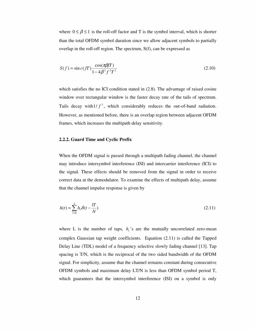
2.2.2. Guard Time and Cyclic Prefix
When the OFDM signal is passed through a multipath fading channel, the channel
may introduce intersymbol interference (ISI) and intercarrier interference (ICI) to
the signal. These effects should be removed from the signal in order to receive
correct data at the demodulator. To examine the effects of multipath delay, assume
that the channel impulse response is given by
�=
−=L
ll N
lTthth
0
)()( δ (2.11)
where L is the number of taps, lh ’s are the mutually uncorrelated zero-mean
complex Gaussian tap weight coefficients. Equation (2.11) is called the Tapped
Delay Line (TDL) model of a frequency selective slowly fading channel [13]. Tap
spacing is T/N, which is the reciprocal of the two sided bandwidth of the OFDM
signal. For simplicity, assume that the channel remains constant during consecutive
OFDM symbols and maximum delay LT/N is less than OFDM symbol period T,
which guarantees that the intersymbol interference (ISI) on a symbol is only
Page 28
13
limited by the previous symbol. The signal at the receiver’s correlator input,
assuming no noise, can be shown as
�=
−=L
ll N
lTtxhtr
0
)()( , (2.12)
where the transmitted OFDM symbol )(tx can be represented as
� �−
−=+ −−=
m
N
NimNi mTts
TmTti
jatx12/
2/,2/ )()
)(2exp()(
π. (2.13)
At the receiver side, received signal is correlated with the complex exponential at
the kth subcarrier frequency over the interval [nT, nT+T] in order to demodulate the
kth subcarrier of the nth OFDM symbol. Therefore, the correlator output can be
represented as [1]
dtT
mTtkjtr
TI
TnT
nTnk �
+ −−= ))(2
exp()(1
,
π. (2.14)
Using (2.12) and (2.13), nkI , can be rewritten as
�
�� �+
=
−
−=+
−−−−−−
=
TnT
nT
m
L
l
N
NimNilnk
dtNlTmTtsT
mTtkj
TNlTmTti
jT
ahI
)/())(2
exp())/(2
exp(1
0
12/
2/,2/,
ππ
Changing the integration limits to [0,T] by replacing t with t+NT and rearranging
the above equation
Page 29
14
�
� � �
−−+−+−−+
=−
−= =
−+
T
m
N
Ni
L
l
NiljlmNink
dtNlTTmntsT
Tmntkj
TTmnti
jT
ehaI
0
12/
2/ 0
/2,2/,
)/)(()))((2
exp()))((2
exp(1 ππ
π
(2.15)
where s(t) is the rectangular window defined on interval [0,T]. It can be seen from
(2.15) that, both m=n and m=n-1 indexes affect the summation over m. After some
manipulations, (2.15) can be written in the form
. (2.16)
In (2.16), the first term is the desired data, scaled by a complex number depending
on the channel taps. The second term represents the intercarrier interference (ICI)
caused by the other subcarriers belonging to the current OFDM symbol. Finally,
the third term represents the intersymbol interference (ISI) caused by the
subcarriers of previous OFDM symbol.
ISI can be avoided by insertion of a guard time at the beginning of each OFDM
symbol. Guard time should be longer than the maximum possible delay spread of
the channel. Let gT be the length of guard interval, insertion of the guard interval
may be seen in Figure 2.3.
���
���
�
−=
−−+
=
−
≠+
+=
−
−+
−+
−=
T
NlTT
L
l
Niljl
inNi
T
NlT
L
l
Niljl
kiinNi
nNk
L
l
Nkljlnk
dtT
tkij
Teha
dtT
tkij
Teha
aeNlhI
/0
/21,2/
/0
/2
,,2/
,2/0
/2,
))(2
exp(1
))(2
exp(1
))/1((
π
π
π
π
π
Page 30
15
Figure 2.3 Insertion of Guard Interval
In this case TTT gs += becomes the new OFDM symbol time. The mth OFDM
symbol is defined in [ ]ss TmmT )1(, + interval and the symbol information is
contained in [ ]sgs TmTmT )1(, ++ interval. Therefore OFDM signal is defined as
[1]
� �−
−=+ −−
−−=
m
N
Nigs
gsmNi TmTts
T
TmTtijatx
12/
2/,2/ )()
)(2exp()(
π (2.17)
where s(t) is the rectangular window defined over interval [0,T]. Hence nth OFDM
symbol can be represented as
��
��
�
+≤≤
+≤≤+−−
= �−
−=+
gss
N
Nisgs
gsmNi
m
TmTtmT
TmtTmTT
TmTtija
tx,0
)1(),)(2
exp()(
12/
2/,2/
π. (2.18)
The correlator output for the kth subcarrier of the nth OFDM symbol is given by
}dtNlTTmTts
T
TmTtkj
T
NlTTmTtij
T
ahI
gs
Tn
TnT
gsgs
m
L
l
N
NimNilnk
s
gs
)/(
))(2
exp())/(2
{exp(1 )1(
0
12/
2/,2/,
−−−
−−−
−−−
=
�
�� �+
+
=
−
−=+
ππ
Zeros OFDM Symbol
Time
T Tg
Page 31
16
.
(2.19)
In this case there is no ISI and only the index m=n involves the sum. When s(t) is a
rectangular window defined over [0,T], we obtain
� ��
�
≠ =
−+
+=
−
−
+ �
���
� −=
kii
T
NlT
L
l
NiljlnNi
nNk
L
l
Nkljlnk
dtTkijT
eha
aeNlhI
, /0
/2,2/
,2/0
/2,
)/)(2exp(1
)/1(
ππ
π
(2.20)
The first term in (2.20) represents the desired symbol scaled by a complex number
depending on the channel tap coefficients. The second term is the intercarrier
interference (ICI) caused by other subcarriers of the same OFDM symbol.
Therefore, it can be stated that, inserting a guard time between OFDM symbols,
during which no signal is transmitted, only the ISI can be avoided, ICI is still
present.
In order to avoid ICI, the last part of the OFDM symbol can be added to the
beginning of the symbol. This part is called the cyclic prefix. Insertion of a cyclic
prefix to the OFDM symbol can be represented as in Figure 2.4.
Figure 2.4 Insertion of Cyclic Prefix
Cyclic Prefix
Time
T Tg
OFDM Symbol
})/)(()))((2
exp(
)))((2
{exp(112/
2/ 0 0
/2,2/
dtNlTTmntsT
Tmntkj
TTmnti
jT
eha
ss
m
N
Ni
L
l
TsNilj
lmNi
−−+−+−
−+=� � � �−
−= =
−+
π
ππ
Page 32
17
In this case, transmitted OFDM signal can be expressed as
� �−
−=+ −
−−=
m
N
Nis
gsmNi mTts
T
TmTtijatx
12/
2/,2/ )()
)(2exp()(
π (2.21)
where s(t) is the rectangular window defined over [0,Ts]. Hence the nth OFDM
symbol is given by
�−
−=+ +≤≤
−−=
12/
2/,2/ )1(),
)(2exp()(
N
Niss
gsnNin TntnT
T
TnTtijatx
π. (2.22)
Then the correlator output for the kth subcarrier of the nth OFDM symbol is
})/)(()))((2
exp(
)))((2
{exp(1
00
/212/
2/,2/,
dtNlTTTmntsT
Tmntkj
TTmnti
jT
ehaI
gss
Ts
m
L
l
Niljl
N
NimNink
−+−+−+
−
−+= �� ��
=
−−
−=+
π
ππ
(2.23)
Since the rectangular window is defined over [0,Ts], the correlator output can be
expressed as
���
�
−
+=
=
−
≠+
=+
−
TL
l
Niljl
kiinNi
L
lnNk
Nkljlnk
dtTkijT
eha
aehI
00
/2
,,2/
0,2/
/2,
)/)(2exp(1 ππ
π
nNk
L
l
Nkljl aeh ,2/
0
/2+
=
− �
���
�= � π (2.24)
which contains only the desired symbol, free from intercarrier interference (ICI)
and intersymbol interference (ISI). Therefore, by inserting a guard time longer than
the maximum delay spread of the channel and by cyclically extending the OFDM
Page 33
18
symbol over the guard time eliminates both the ICI and ISI completely and the
channel appears to be flat fading for each subcarrier.
If we take ν+N samples from xn(t) given by (2.22) at a sampling rate of
sTN /)( ν+ where TNTg /=ν (Tg is selected properly in order to obtain an integer
value ofν ), then we have
[ ] �−
−=+
−−=12/
2/,2/ ),2exp(
N
NinNin N
vkijaky π 10 −+≤≤ vNk . (2.25)
If we focus on (2.25), it can be observed that, ν+N samples of OFDM symbol
can be generated by taking N-point IDFT of sequence {ai} and then adding last ν
samples to the beginning of the IDFT output.
Let un[k] represent the N-point IDFT of sequence {ai,n} given by
[ ] �−
−=+ −=
12/
2/,2/ )2exp(
N
NinNin N
kijaku π , 10 −≤≤ Nk . (2.26)
Comparing (2.25) and (2.26), it can be seen that
, -[ku[k]y nn ]= ν 1−+Ν≤≤ νν k . (2.27)
Also for ,ν<k
)],−= kν(-[Nu[k]y nn ν<≤ k0 . (2.28)
Equations (2.27) and (2.28) demonstrate that, OFDM symbol can be reconstructed
from the samples of IDFT output, together with the addition of the cyclic prefix.
Page 34
19
2.2.3. Synchronization
An OFDM receiver needs to perform synchronization operation prior to subcarrier
demodulation. Two types of synchronization are needed. First, symbol boundaries
are determined and then proper sampling instants are found out in order to
minimize ICI and ISI effects. Second step of synchronization is used to eliminate
the carrier frequency offset on the received signal. In an OFDM system, the
orthogonality assumption is valid only if the transmitter and the receiver use
exactly the same frequency. Any frequency offset results in intercarrier
interference (ICI). Additionally, a practical oscillator does not produce a carrier at
exactly one frequency, instead it produces a carrier that is phase modulated by
random phase jitter. Hence, frequency is never perfectly constant resulting in some
ICI in OFDM receiver.
In this section, sensitivity of OFDM systems to phase noise, frequency offset and
timing errors should be examined. Then two synchronization techniques used in
OFDM systems will be introduced.
2.2.3.1. Sensitivity to Phase Noise
In [14], power spectrum density of an oscillator signal with phase noise is modeled
by a Lorentzian spectrum, which is equal to the squared magnitude of a first order
lowpass filter transfer function. The single sided spectrum is given by
21
2
1
/||1
/1)(
fff
ffS
c−+=
π . (2.29)
In (2.30), 1f is the 3 dB linewidth of the oscillator signal and cf is the carrier
frequency.
Page 35
20
Phase noise has two main effects. First, the phase noise results in attenuation and
rotation of the received signal. Second and more important effect is the ICI,
because phase noise changes the 1/T separation between subcarriers in the
frequency domain. In [14], the degradation in SNR caused by phase noise is given
as
0
410ln6
11NE
TSNR sloss πβ≈ (2.30)
where β is the 3 dB one sided bandwidth of the power spectrum density of the
carrier, T is the symbol period and Es/ N0 is the symbol-to-noise energy ratio. From
(2.30), it is seen that phase noise degradation is proportional with the ratio of
subcarrier bandwidth ( β ) and the subcarrier spacing (1/T). It can be seen from
[14] that, for a negligible SNR degradation of less than 0.1 dB, the 3 dB phase
noise bandwidth has to be about 0.1 to 0.01 percent of the subcarrier spacing,
depending on the modulation. For example, if 64 QAM modulation is used in an
OFDM system with a subcarrier spacing of 300 kHz, the 3 dB bandwidth should be
30 Hz at most.
2.2.3.2. Sensitivity to Frequency Offset
As stated in [14], the degradation in SNR caused by a frequency offset which is
small relative to subcarrier spacing can be approximated as
0
2)(10ln3
10NE
fTSNR sloss ∆≈ π . (2.31)
As shown in [14], for a negligible degradation of about 0.1 dB, maximum tolerable
frequency offset is less than 1% of subcarrier frequency. For example, for an
OFDM system at a carrier frequency of 5 GHz and a subcarrier spacing of 300
kHz, the oscillator accuracy needs to be 3 kHz or 0.6 ppm. Initial frequency error
Page 36
21
of a low cost oscillator will not meet this requirement. Therefore, a frequency
synchronization technique has to be applied before the FFT block of the receiver.
2.2.3.3. Sensitivity to Timing Errors
OFDM is more robust to timing errors relative to phase noise and frequency
offsets. The symbol timing offset may vary over an interval equal to the guard time
without causing ICI and ISI. Interferences occur only when the FFT interval
extends over a symbol boundary or extends over the roll-off region of a system.
Therefore, we can state that OFDM demodulation is quite insensitive to timing
errors. However, in order to achieve the best possible multipath robustness, there is
an optimal timing instant. Deviation from this timing instant increases the
sensitivity to delay spread, so the system can handle less delay spread than it is
designed for. To minimize this sensitivity, the system should be designed such that
the timing error is small compared to the guard interval.
2.2.3.4. Synchronization Techniques
There are several OFDM synchronization techniques used in the literature. This
section describes the synchronization methods in two categories: Synchronization
Using Cyclic Extension and Synchronization Using Special Training Symbols.
2.2.3.4.1. Synchronization Using Cyclic Extension
Because of cyclic prefix, the first Tg seconds of an ODFM symbol is the same as
the last Tg seconds of the symbol. This property can be used for both timing and
frequency synchronization by using a system given in Figure 2.5. This system
correlates a Tg long part of the OFDM signal with a part that is T seconds delayed
[15].
Page 37
22
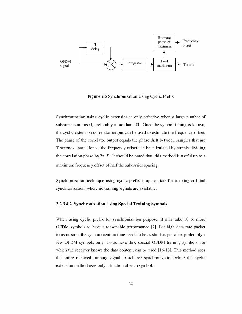
Figure 2.5 Synchronization Using Cyclic Prefix
Synchronization using cyclic extension is only effective when a large number of
subcarriers are used, preferably more than 100. Once the symbol timing is known,
the cyclic extension correlator output can be used to estimate the frequency offset.
The phase of the correlator output equals the phase drift between samples that are
T seconds apart. Hence, the frequency offset can be calculated by simply dividing
the correlation phase by Tπ2 . It should be noted that, this method is useful up to a
maximum frequency offset of half the subcarrier spacing.
Synchronization technique using cyclic prefix is appropriate for tracking or blind
synchronization, where no training signals are available.
2.2.3.4.2. Synchronization Using Special Training Symbols
When using cyclic prefix for synchronization purpose, it may take 10 or more
OFDM symbols to have a reasonable performance [2]. For high data rate packet
transmission, the synchronization time needs to be as short as possible, preferably a
few OFDM symbols only. To achieve this, special OFDM training symbols, for
which the receiver knows the data content, can be used [16-18]. This method uses
the entire received training signal to achieve synchronization while the cyclic
extension method uses only a fraction of each symbol.
OFDM signal Timing
Estimate phase of
maximum Frequency offset
Integrator Find maximum
T delay
Page 38
23
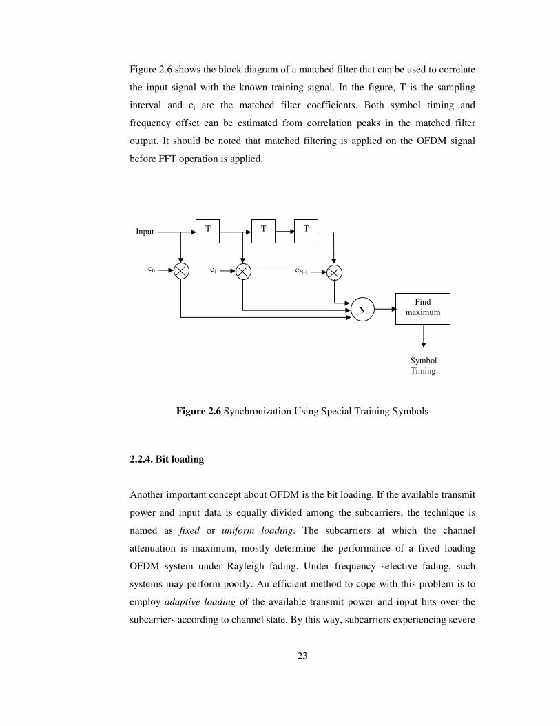
Figure 2.6 shows the block diagram of a matched filter that can be used to correlate
the input signal with the known training signal. In the figure, T is the sampling
interval and ci are the matched filter coefficients. Both symbol timing and
frequency offset can be estimated from correlation peaks in the matched filter
output. It should be noted that matched filtering is applied on the OFDM signal
before FFT operation is applied.
Figure 2.6 Synchronization Using Special Training Symbols 2.2.4. Bit loading
Another important concept about OFDM is the bit loading. If the available transmit
power and input data is equally divided among the subcarriers, the technique is
named as fixed or uniform loading. The subcarriers at which the channel
attenuation is maximum, mostly determine the performance of a fixed loading
OFDM system under Rayleigh fading. Under frequency selective fading, such
systems may perform poorly. An efficient method to cope with this problem is to
employ adaptive loading of the available transmit power and input bits over the
subcarriers according to channel state. By this way, subcarriers experiencing severe
Input
c0
T T T
c1 cN-1
� Find
maximum
Symbol Timing
Page 39
24
fading are loaded with a small number of bits, or may not be used at all. The
advantage it provides in increasing the capacity can be computed for fading
channels as described in [26].
2.2.5. Peak-to-Average Power Ratio (PAPR)
Amplitude of the OFDM signal has an almost Rayleigh distribution and exhibits
strong fluctuations. Therefore, the resultant Peak-to-Average Power Ratio (PAPR)
can be rather high. In the worst case, PAPR of an OFDM system with N
subchannels may reach up to a value of N. High PAPR value has some
disadvantages for practical implementations and needs to be reduced to an
acceptable level. In the literature various methods are proposed for the purpose of
PAPR reduction. Next chapter deals with PAPR problem and the proposed
solutions in more detail.
2.3. Applications of OFDM
OFDM is used as the transmission technique in digital audio and television
broadcasting applications, and in wireless LAN applications. This section describes
the main applications of OFDM.
2.3.1. Digital Audio Broadcasting (DAB)
DAB is the successor of current analog audio broadcasting based on AM and FM
and offers improved sound quality, comparable to that of CD quality, new data
services and a higher spectrum efficiency. DAB was standardized in 1995 by the
European Telecommunications Standards Institute (ETSI) as the first standard to
use OFDM [32, 33]. The basis for this standard was the specification developed by
the European Eureka 147 DAB project, which started in 1988.
Page 40
25
DAB has four transmission modes using different sets of OFDM parameters, which
are listed in Table 2.1. The parameters for modes I to III are optimized for use in
specific frequency bands, while mode IV was introduced to provide a better
coverage range at the cost of an increased vulnerability to Doppler shifts. DAB can
be operated above 30 MHz and the upper limits of the carrier frequency are given
in Table 2.1.
Table 2.1 DAB OFDM Parameters
Mode I Mode II Mode III Mode IV
Number of subcarriers 1536 384 192 768
Subcarrier spacing 1 kHz 4 kHz 8 kHz 2 kHz
Symbol time 1.246 ms 0.3115 ms 0.1558 ms 0.623 ms
Guard time 0.246 ms 0.0615 ms 0.0308 ms 0.123 ms
Carrier frequency < 375 MHz < 1.5 GHz < 3 GHz < 1.5 GHz
Transmitter separation < 96 km < 24 km < 12 km < 48 km
One important reason to use OFDM for DAB is the possibility to use a single
frequency network, which greatly enhances the spectrum efficiency. As long as the
delay between two signals is smaller than the guard time, no ISI and ICI occur due
to the simultaneous transmission.
The transmitted data consists of a number of audio signals, sampled at 48 kHz with
an input resolution up to 22 bits. The digital audio signal is compressed to a rate in
the range of 32 to 384 kbps, depending on the desired quality. Transmission is
done on 24 ms long frames. The start of a frame is indicated by a null symbol,
which is a silence period that is slightly larger than the duration of an OFDM
symbol. Then a reference OFDM symbol is sent which serves as the starting point
for the differential decoding of the QPSK modulated subcarriers.
Page 41
26
The digital input data is encoded by a rate 1/4 convolutional code with a constraint
length of 7. The coding rate can be increased up to 8/9 by puncturing. This yields a
total maximum data rate of approximately 2.2 Mbps. The coded data are then
interleaved in frequency domain by distributing the input data over subcarriers,
which avoids large burst errors in the case of a deep fade affecting a group of
subcarriers.
2.3.2. Terrestrial Digital Video Broadcasting
Research on a digital system for TV broadcasting has been carried out since the
late 1980s. In 1993, a pan-broadcasting industry group started the Digital Video
Broadcasting (DVB) project. Within this project, a set of specifications was
developed for the delivery of digital television over satellites, cable and through
terrestrial transmitters. The terrestrial DVB system was standardized in 1997 [31,
34].
Terrestrial DVB uses OFDM with two possible modes, using 1705 and 6817
subcarriers, respectively. These modes are referred to us 2k and 8k modes, which
correspond to the sizes of IFFT and FFT blocks used in multicarrier modulation
and demodulation. The symbol period of 8k system is about 896 µs, while the
guard time may have four different values between 28 to 224 µs. The
corresponding values for the 2k system are four times smaller.
At the DVB-T transmitter, the input data is divided into groups of 188 bytes, which
are scrambled and coded by an outer shortened (204,188) Reed-Solomon (RS)
code over GF(256). This code can correct up to 8 byte errors in a frame of 204
bytes. The coded bits are then interleaved and then coded again by a rate 1/2
convolutional code, with a constraint length of 7. The coding rate can be increased
for higher throughput by puncturing to 2/3, 3/4, 5/6 or 7/8. The encoded bits are
then interleaved by an inner interleaver and then mapped onto QPSK, 16 QAM or
64 QAM symbols.
Page 42
27
The receiver side employs coherent detection of QAM signals which requires the
estimation of channel effects. This is accomplished by using pilot subcarriers. For
the 8k mode, in each symbol there are 768 pilots, so 6048 subcarriers are allocated
to data traffic. The 2k mode has 192 pilots and 1512 data subcarriers. The position
of pilots varies from symbol to symbol with a pattern that repeats after 4 OFDM
symbols. The pilots allow the receiver to estimate the channel both in frequency
and time.
2.3.3. Magic WAND
The Magic WAND (Wireless ATM Network Demonstrator) project was a part of
European ACTS (Advanced Communications Technology and Servers) program
[25]. The Magic WAND consortium members implemented a prototype wireless
ATM network based on OFDM. This prototype had a large impact on
standardization activities in the 5 GHz band. The wireless ATM application based
on OFDM forms the basis for the standardization of the HYPERLAN type II
physical layer.
The main parameters of the WAND physical layer are listed in Table 2.2. The
number of subcarriers is 16, with a guard time of 400 ns. With this guard time, rms
delay spreads up to 100 ns are completely tolerated without employing
equalization. While this is sufficient for most of the office buildings, a realistic
product would require more delay spread robustness in order to cover large office
buildings and factory halls.
As can be seen from Table 2.2, the subcarrier modulation is 8 PSK with a symbol
rate of 13.3 Msymbols/s, yielding a raw data rate of 40 Mbps. The rate 1/2
complementary coding reduces the net rate to 20 Mbps. The subcarrier spacing is
1.25 MHz, which gives a total bandwidth of 20 MHz. The packet preamble is 8.4
µs in duration and consists of one OFDM symbol, repeated 7 times. This preamble
Page 43
28
is used for packet detection, automatic gain control, frequency offset estimation,
symbol timing and channel estimation. Transmission is done on half-slots, which
consists of 9 OFDM symbols, carrying 27 bytes. An ATM cell is mapped on two
consecutive half-slots, which form a full-slot. Of the 54 bytes carried on one full-
slot, 53 bytes are allocated to ATM cell traffic and remaining 1 byte is reserved for
physical layer control signaling.
Table 2.2 Main Parameters of the WAND OFDM Modem
Number of subcarriers 16
Modulation 8-PSK
Coding Rate 1/2, length 8 complementary coding
Net bit rate 20 Mbps
Symbol time 1.2 µs
Guard time 0.4 µs
Windowing Raised cosine, with 0.2 roll-off
Subcarrier spacing 1.25 MHz
Training length 7 symbols
Carrier frequency 5.2 GHz
Peak output power 1 W
The WAND modem uses complementary codes for both forward-error correction
and PAP reduction. Length 8 complementary codes are used, with 4 8-PSK
symbols input, generating eight complex code outputs. By taking the IFFT of this
complex coded output, an OFDM signal with a low PAP ratio is obtained. To
encode 16 subcarriers, two length 8 codes are interleaved, which maximizes the
benefits of frequency diversity. The minimum distance of the length 8 code is 4
symbols, and hence three arbitrary subcarriers can be erased without causing
errors, provided that the data loaded onto the remaining subcarriers are not in error.
Page 44
29
The performance of Magic WAND modem under Rayleigh fading was reported in
[2]. According to the results provided in [2] , for a delay spread of 50 ns, an
average SNR of approximately 30 dB is required to reach 10-6 BER, without
antenna diversity. At these average SNR, the packet error rate is about 5x10⁻⁵.
2.3.4. IEEE 802.11, HYPERLAN/2 and MMAC Wireless LAN Standards
Since the beginning of 90’s, wireless local area networks (WLAN) for the 900
MHz, 2.4GHz and 5 GHz ISM (Industrial Scientific and Medical) bands have been
available, based on proprietary techniques. In June 1997, the Institute of Electrical
and Electronics Engineers (IEEE) approved an international interoperability
standard [35]. The standard specifies medium access control (MAC) procedures
and three different physical layers (PHY). Two of the specified PHYs are radio
based using 2.4 GHz band and the third uses infrared light. All PHYs support a
data rate of 1 Mbps and optionally 2 Mbps.
User demand for higher bit rates and the international availability of the 2.4 GHz
band has encouraged the development of a higher speed extension to the 802.11
standard. In July 1998, a proposal was selected for standardization, which
describes a PHY providing a basic rate of 11 Mbps and a fall back rate of 5.5
Mbps. A second IEEE 802.11 working group has moved on to standardize yet
another PHY option, which offers higher bit rates in the 5.2 GHz band. This
development was motivated by the adoption, in January 1997, by the US Federal
Communications Commission (FCC), of a modification to FCC part 15 rules. The
modification makes available 300 MHz spectrum in the 5.2 GHz band, intended for
use by a new category of unlicensed equipment called “Unlicensed National
Information Infrastructure (UNII)” devices.
Like the IEEE 802.11 standard, the European ETSI HYPERLAN type I [36]
specifies both MAC and PHY layers. Unlike 802.11, however, there is no
HYPERLAN type I compliant products available in the market. A newly formed
Page 45
30
ETSI working group called “Broadband Radio Access Networks (BRAN)” has
started to work on extensions to HYPERLAN standard which is referred as
HYPERLAN type II [37].
In Japan, equipment manufacturers and service providers are cooperating in the
Multimedia Mobile Access Communication (MMAC) project to define new
wireless standards similar to those of IEEE 802.11 and ETSI BRAN. Additionally,
MMAC is also looking into possibility for ultra-high speed wireless indoor LANs
supporting large volume data transmission at speeds up to 156 Mbps using EHF
band (30-300 GHz).
In July 1988, the IEEE 802.11 standardization group decided to select OFDM as
the basis for their new 5 GHz standard, called IEEE 802.11a, targeting a range of
data rates from 6 up to 54 Mbps [38]. This new standard is the first one which uses
OFDM in packet-based high speed data communications. Following the IEEE
802.11 decisions, ETSI BRAN and MMAC also adopted OFDM for their physical
layer standards. The three bodies have worked in close cooperation since then to
make sure that the differences among the various standards are kept at a minimum
level, thereby enabling world wide equipment manufacturing.
Table 2.3 lists the main parameters of OFDM physical layer adopted in all these
standards with some minor changes. A key parameter that largely determines the
choice of the other parameters is the guard interval of 800 ns. This provides
robustness to rms delay spreads up to several hundreds of nanoseconds. In practice,
this means that any indoor environment including large factory buildings can be
covered.
To limit the relative amount of power and time spent on the guard time, the symbol
duration is chosen to be 4 µs. This determines the subcarrier spacing at 312.5 kHz.
By using 48 data subcarriers, uncoded data rates of 12 to 72 Mbps can be achieved
by using variable modulation types from BPSK to 64 QAM. In addition to 48 data
Page 46
31
subcarriers, each OFDM symbol contains an additional 4 pilot subcarriers, which
can be used to track the residual carrier frequency offset that remains after an
initial frequency correction during the training phase of the packet. The training
phase of the packet consists of three parts, a 8 µs long first part consisting of 10
short symbols to be used in AGC and coarse frequency offset estimation, followed
by another 8 µs part consisting of two OFDM symbols used for fine frequency
offset estimation, symbol timing and channel estimation purposes and a 4 µs final
part consisting of one OFDM symbol used primarily for physical layer signaling
(indicating coding rate, modulation type, packet length etc. that are used in the rest
of the packet carrying the user data).
To correct the errors encountered in deep fades, forward-error correction across the
subcarriers is used with variable coding rates, yielding net data rates from 6 up to
54 Mbps. The main code is a rate 1/2, constraint length 7 convolutional code and
higher coding rates can be obtained by puncturing the mother code to 2/3 and 3/4.
The rate 2/3 code is used together with 64 QAM to obtain a net data rate of 48
Mbps. The rate 1/2 code is used in conjunction with BPSK, QPSK and 16 QAM,
yielding net data rates of 6,12 and 24 Mbps, respectively. Finally, the rate 3/4 code
is used in conjunction with BPSK, QPSK,16 QAM and 64 QAM, yielding net data
rates of 9,18,36 and 54 Mbps, respectively. As an example of the error rate
performance of the receiver under Rayleigh fading, it was reported in [2] that, for
the 24 Mbps mode, in order to obtain a packet error rate of 10-4, an average SNR of
about 22dB is required for an rms delay spread of 100 ns without antenna diversity.
Page 47
32
Table 2.3 Main Parameters of the OFDM physical layer standards (IEEE 802.11a,
ETSI HYPERLAN type II and MMAC)
Data Rate 6, 9, 12, 18, 24, 36, 48, 54 Mbps
Modulation BPSK, QPSK, 16 QAM, 64 QAM
Coding Rate 1/2, 2/3, ¾
Number of subcarriers 52
Number of pilots 4
OFDM symbol duration 4 µs
Guard interval 800 ns
Subcarrier spacing 312.5 kHz
Total bandwidth 16.56 MHz
Channel spacing 20 MHz
Maximum transmit
Power
1 W (802.11 at 2.4-2.4835 and 5.725-5.825 GHz
Bands)
250 mW (802.11 at 5.25-5.35 GHz)
50 mW (802.11 at 5.15-5.25 GHz)
100 mW (HYPERLAN at 2.4-2.4835 GHz)
10 mW (MMAC at 2.471-2.497 GHz)
Page 48
33
CHAPTER 3
PAPR REDUCTION TECHNIQUES 3.1. Introduction
OFDM signal is essentially the sum of many independently modulated sine waves
and its amplitude has an almost Rayleigh distribution. Amplitude of OFDM signal
exhibits strong fluctuations and the resultant Peak-to-Average Power Ratio (PAPR)
can be rather high. In the worst case, N signals with the same phase are added up
resulting in a peak power that is N times the average power; i.e. PAPR may reach a
value of N. For an OFDM system with 256 subcarriers, PAPR may reach to 24 dB.
High value of PAPR brings disadvantages like an increased complexity of A/D and
D/A converters and a reduced efficiency of RF power amplifiers. In a practical
system, before transmission, OFDM signal is passed through a power amplifier
that is always peak power limited. If the squared magnitude of the OFDM signal is
larger than the saturation point of the power amplifier at any time instant, then the
signal will be clipped. Clipping destroys the orthogonality between subcarriers
resulting in an increase in the BER when compared with the nonclipped case [19].
PAPR is important for OFDM since it is a measure of the clipping probability.
In the literature various methods are proposed for the purpose of PAPR reduction.
In this chapter, some PAPR reducing methods will be discussed. First section
represents the signal distorting methods such as clipping, peak windowing and peak
cancellation. Later, scrambling techniques will be mentioned and the most
frequently used two scrambling methods, selected mapping and partial transmit
sequences, will be described in detail. Last section should consider coding
techniques used to decrease PAPR value of the OFDM signal.
Page 49
34
3.2. Clipping and Peak Windowing
The simplest way to reduce PAPR is to clip the signal such that the peak amplitude
becomes limited to a desired level [20]. Figure 3.1 shows the clipping operation.
Clipping is the simplest solution in terms of algorithm complexity; however there
are two basic problems associated this technique. First problem is the introduction
of self interference which degrades the Bit Error Rate (BER) performance. Second,
nonlinear distortion of OFDM signal increases the out-of-band radiation. This
effect can be clarified by considering clipping operation as a multiplication of the
OFDM signal by a rectangular window function. Amplitude of the rectangular
function equals 1 if the OFDM amplitude is below the threshold and smaller than 1
if the amplitude exceeds the threshold. The spectrum of the clipped OFDM signal
is the spectrum of the input OFDM signal convolved with the spectrum of the
windowing function. Therefore, the out-of-band characteristics are mainly
determined by the wider spectrum of the two, which is the spectrum of the
rectangular window function. The spectrum of a rectangular function has a very
slow roll of that is proportional to the reciprocal of the frequency.
Figure 3.1 Clipping of OFDM Signal
Page 50
35
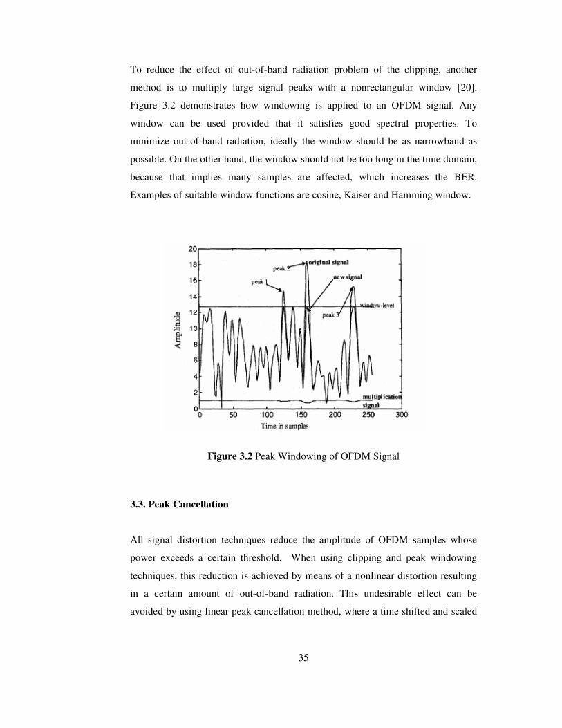
To reduce the effect of out-of-band radiation problem of the clipping, another
method is to multiply large signal peaks with a nonrectangular window [20].
Figure 3.2 demonstrates how windowing is applied to an OFDM signal. Any
window can be used provided that it satisfies good spectral properties. To
minimize out-of-band radiation, ideally the window should be as narrowband as
possible. On the other hand, the window should not be too long in the time domain,
because that implies many samples are affected, which increases the BER.
Examples of suitable window functions are cosine, Kaiser and Hamming window.
Figure 3.2 Peak Windowing of OFDM Signal
3.3. Peak Cancellation
All signal distortion techniques reduce the amplitude of OFDM samples whose
power exceeds a certain threshold. When using clipping and peak windowing
techniques, this reduction is achieved by means of a nonlinear distortion resulting
in a certain amount of out-of-band radiation. This undesirable effect can be
avoided by using linear peak cancellation method, where a time shifted and scaled
Page 51
36
reference function is subtracted from the signal, such that each subtracted reference
function reduces the peak power of at least one signal sample. Furthermore,
selecting a reference function with approximately the same bandwidth as the
transmitted signal can assure that the peak power reduction does not cause an
increase in the out-of-band radiation. An example of a suitable reference function
is the multiplication of a sinc function and a raised cosine function. If the
windowing function is same as the function used for OFDM symbol windowing,
then the reference function has the same bandwidth as of the OFDM signal. Hence,
peak cancellation will not degrade the out-of-band spectrum properties. By making
the reference signal window narrower, a tradeoff can be made between the
complexity of the peak cancellation calculations and an increase in out-of-band
power. The peak cancellation technique was described in [21].
Peak cancellation can be done digitally after generation of the digital OFDM
symbols. It involves a peak power detector, a comparator to see if the peak power
exceeds the threshold and a scaling of the peak and surrounding samples. Figure
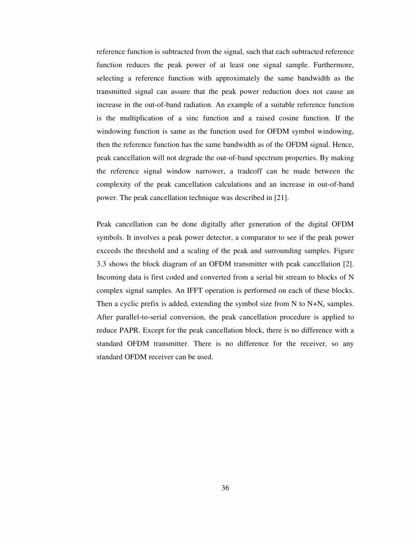
3.3 shows the block diagram of an OFDM transmitter with peak cancellation [2].
Incoming data is first coded and converted from a serial bit stream to blocks of N
complex signal samples. An IFFT operation is performed on each of these blocks.
Then a cyclic prefix is added, extending the symbol size from N to N+Nc samples.
After parallel-to-serial conversion, the peak cancellation procedure is applied to
reduce PAPR. Except for the peak cancellation block, there is no difference with a
standard OFDM transmitter. There is no difference for the receiver, so any
standard OFDM receiver can be used.
Page 52
37
Figure 3.3 OFDM Transmitter with Peak Cancellation
In Figure 3.3, the peak cancellation was done after parallel-to-serial conversion
stage. It is possible to implement peak cancellation immediately after the IFFT
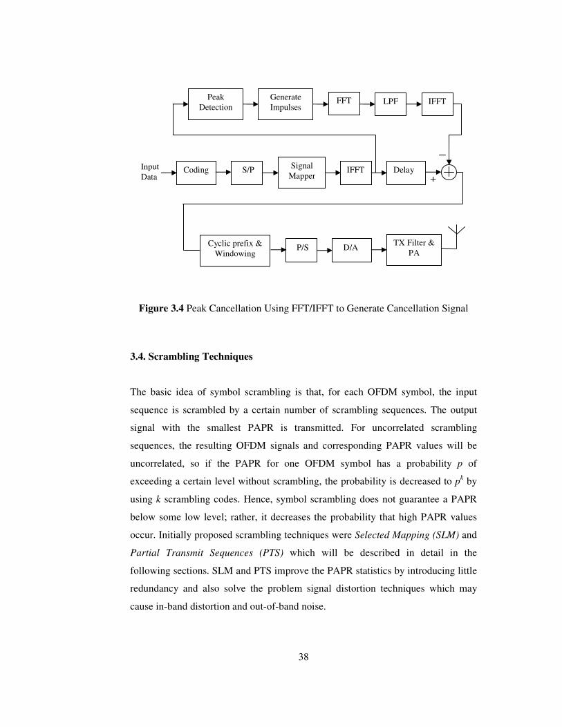
stage, as given in Figure 3.4 [2]. In this case, the cancellation is done on a symbol-
by-symbol basis. An efficient way to generate the cancellation signal without using
a stored reference function is to use a lowpass filter in the frequency domain. In
Figure 3.4, for each OFDM symbol, it is detected which samples exceed a certain
amplitude. Then, for each signal peak, an impulse is generated whose phase equals
the peak phase and whose amplitude equals the peak amplitude minus the desired
maximum amplitude. The impulses are then lowpass filtered on a symbol-by-
symbol basis. Lowpass filtering is achieved in the frequency domain by taking the
FFT, setting all outputs to zero whose frequencies exceed the frequency of the
highest subcarrier, and then transforming the signal back by an IFFT.
Peak cancellation method seems to be a fundamentally different method than
clipping and peak windowing. However, in [2] it is shown that peak cancellation is
identical to clipping followed by filtering. This method was proposed as a PAPR
reduction technique in [22].
Input Data
Coding S/P Signal Mapper
IFFT Cyclic prefix & Windowing
P/S Peak Cancellation
D/A TX Filter & PA
Page 53
38
Figure 3.4 Peak Cancellation Using FFT/IFFT to Generate Cancellation Signal
3.4. Scrambling Techniques
The basic idea of symbol scrambling is that, for each OFDM symbol, the input
sequence is scrambled by a certain number of scrambling sequences. The output
signal with the smallest PAPR is transmitted. For uncorrelated scrambling
sequences, the resulting OFDM signals and corresponding PAPR values will be
uncorrelated, so if the PAPR for one OFDM symbol has a probability p of
exceeding a certain level without scrambling, the probability is decreased to pk by
using k scrambling codes. Hence, symbol scrambling does not guarantee a PAPR
below some low level; rather, it decreases the probability that high PAPR values
occur. Initially proposed scrambling techniques were Selected Mapping (SLM) and
Partial Transmit Sequences (PTS) which will be described in detail in the
following sections. SLM and PTS improve the PAPR statistics by introducing little
redundancy and also solve the problem signal distortion techniques which may
cause in-band distortion and out-of-band noise.
+ Input Data
Coding S/P Signal Mapper
IFFT
Cyclic prefix & Windowing
P/S D/A TX Filter & PA
Delay
Peak Detection
Generate Impulses
FFT LPF IFFT
Page 54
39
3.4.1. Selected Mapping
Assume that an OFDM symbol is scrambled by M different scrambling sequences.
Then M statistically independent OFDM symbols represent the same information.
If the symbol with the lowest PAPR is selected for transmission, the probability
that the PAPR value of the selected symbol (PAPRlow) exceeds a certain threshold
z is given by
P{PAPRlow > z}= (P{PAPRinit > z})M (3.1)
where PAPRinit is the PAPR value of the original symbol. The key idea of Selected
Mapping (SLM) is to choose one particular signal that exhibits the lowest PAPR
value among M candidates, all representing the same information. The block
diagram of SLM is shown in Figure 3.5.
Figure 3.5 Block Diagram of Selected Mapping Method
a˜µ
a µ(M)
a µ(2)
a µ(1)
Aµ(M)
Aµ(2)
Aµ(1)
P(M)
P(2)
P(1)
Aµ
IFFT
.
.
.
Selection of a
desirable symbol
.
.
.
.
.
.
.
.
IFFT
IFFT
Page 55
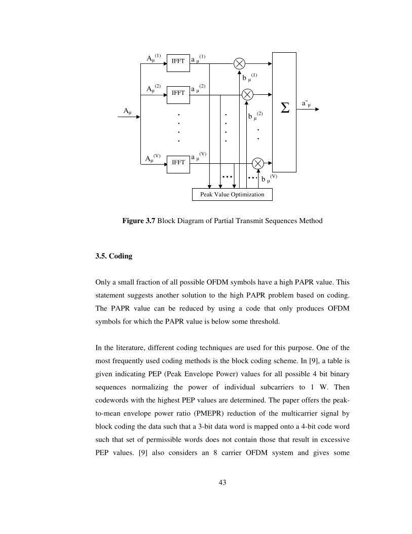
40
In Figure 3.5, the M independent OFDM symbols aµ(1).... aµ
(M) represent the same
information and the symbol a˜µ with the lowest PAPR is selected for transmission.
The way of choosing P(k) vectors is as follows
P(k)=[P1(k), ..., PN
(k) ] ,
with Pv(k) = ej�
v(k) where �v
(k) ∈ [0, 2π), 1� v � N, 1� k <M. After mapping the
information to the subcarrier amplitude Aµ,v, each OFDM symbol is multiplied
with the M vector P(k), resulting in a set of M different OFDM symbols Aµ(k) with
components represented by [7]
Aµ,v(k) = Aµ,v. Pv
(k), 1� v � N, 1� k � M (3.2)
All new M OFDM symbols are transformed into time domain defined by
aµ(k) = IFFT { Aµ
(k)}. (3.3)
Finally, the symbol with the lowest PAPR is selected, which is represented as a˜µ in
Figure 3.5. Notice that, increasing the number distinct vectors used for scrambling
(i.e. M), the PAPR reduction amount is increased.
In order to implement SLM effectively, the components of Pv(k) should consist of
{±1, ±j} as multiplication with these components can be implemented simply by
interchanging, adding and subtracting real and imaginary parts. For the receiver to
demodulate the data, it should know which vector is used at the transmitter to
scramble the data. The most important disadvantage of SLM appears at this stage,
the transmitter has to transfer side information to distinguish the vector used for
scrambling. The number of required bits to be transmitted as side information is
� M2log . Side information should be protected carefully; hence it should be sent
from a secure channel, which increases system cost.
Page 56
41
In [8], a method is suggested in order to avoid transmission of side information in a
SLM system. In this technique, to generate M different transmit sequences a(k), 1�
k � M representing the same information word q, labels b(k) are inserted as a prefix
to q. The labels are M different binary vectors of length � M2log . The
concatenated word vector of the label and the information word is fed into a
scrambler. The labels are hence used to drive the scrambler into one of the M
different states before scrambling the information word q itself. Finally, the
specific transmit sequence number u˜, which possesses the lowest peak power, is
selected for transmission. This method removes the need for side information,
however as classical SLM approach, it reduces the probability of the OFDM
symbol PAPR to exceed a certain threshold, does not guarantee a certain reduction
value.
3.4.2. Partial Transmit Sequences
The main principle of Partial Transmit Sequences (PTS) method is to partition an
OFDM symbol Aµ into V disjoint subblocks Aµ(k) (k=1, …, V). The simple and
effective method is to divide an OFDM symbol into subblocks of the same size as
shown in Figure 3.6. All subcarrier positions in Aµ(k), which are represented in
another subblock, are set to zero. Therefore, Aµ equals to the sum of all subblocks
as given by
�=
=V
k
kAA1
)(µµ (3.4)
Figure 3.7 gives the block diagram of a PTS system. After partitioning the OFDM
symbol, each Aµ(k) is multiplied by a complex-valued phase rotation factor b µ
(k),
where b µ(k) = ej�
µ(k) where �µ
(k) ∈[0, 2π), 1� k � V. A phase rotation of all
subcarriers included in the subblock k by the same angle � µ(k) = arg(b µ
(k)) is
performed. To calculate time domain signal a˜µ, the subblocks are transformed by
V separate and parallel IFFTs as following [6]
Page 57
42
a˜µ = �=
V
k
kk AIFFTb1
)()( }{ µµ = �=
V
k
kk ab1
)()(µµ . (3.5)
Figure 3.6 Subblock Configuration for Partial Transmit Sequences Method
From Figure 3.7, peak value of OFDM symbol can be reduced by suitably
selecting the phase rotation parameter bµ(k) in the peak value optimization block.
To implement PTS effectively, the components of bµ(k) should consist of {±1, ±j}.
In order to demodulate the received data, the receiver has to know information
about bµ(k), transmitter therefore has to transfer the side information as the case
with SLM technique.
.
.
.
.
k Aµ
(1)
k Aµ
(2)
k Aµ
(V)
Page 58
43
Figure 3.7 Block Diagram of Partial Transmit Sequences Method
3.5. Coding
Only a small fraction of all possible OFDM symbols have a high PAPR value. This
statement suggests another solution to the high PAPR problem based on coding.
The PAPR value can be reduced by using a code that only produces OFDM
symbols for which the PAPR value is below some threshold.
In the literature, different coding techniques are used for this purpose. One of the
most frequently used coding methods is the block coding scheme. In [9], a table is
given indicating PEP (Peak Envelope Power) values for all possible 4 bit binary
sequences normalizing the power of individual subcarriers to 1 W. Then
codewords with the highest PEP values are determined. The paper offers the peak-
to-mean envelope power ratio (PMEPR) reduction of the multicarrier signal by
block coding the data such that a 3-bit data word is mapped onto a 4-bit code word
such that set of permissible words does not contain those that result in excessive
PEP values. [9] also considers an 8 carrier OFDM system and gives some
... b µ(V)
.
.
.
.
b µ(2)
b µ(1)
...
a˜µ
a µ(V)
a µ(2)
a µ(1)
Aµ(V)
Aµ(2)
Aµ(1)
Aµ
IFFT
� . . . .
.
.
.
.
IFFT
IFFT
Peak Value Optimization
Page 59
44
numerical results such that, if no block coding is used, PMEPR equals 9.03 dB, if
half of the possible codewords are permissible, PMEPR equals 4.45 dB and if
quarter of the possible codewords are permissible PMEPR equals 3.01 dB. These
results are based on an exhaustive search through all possible codewords. The
paper shows significant PEP reductions are possible; however it does not describe
how to perform encoding and decoding operation. Additionally, as described in [9],
the potential of this technique is limited because as the number of carriers and the
number of modulation levels increases, the ratio of the number of permissible
codewords to all codewords must be reduced to achieve a desired PMEPR. On the
other hand, [9] has an important result: Inspection of PEP (Peak Envelope Power)
values for eight carriers with BPSK modulation confirmed that many but not all of
the codewords that resulted in low PEP values were Golay complementary
sequences. However, the few codewords that yielded the minimum PEP were not
Golay complementary sequences. Consequently, using the Golay complementary
sequences would result in a PMEPR greater than the optimum, for a given code
rate. Nevertheless, it would give a code that is open to mathematical encoding and
decoding and may have error detection/correction capability.
It was already mentioned in [23] that the correlation properties of Golay
complementary sequences translate into a relatively small PAPR of 3 dB when the
codes are used to modulate an OFDM signal. For OFDM with a large number of
channels, it may not be feasible to generate a sufficient number of complementary
codes with a length equal to the number of channels. To avoid this problem, [24]
suggests to split the total number of channels and applying a complementary code
to each group of subchannels increasing the code rate at the cost of error correction
capability and PAPR reduction. It may be concluded that, complementary codes
have good properties to serve as both PAPR reduction codes and as forward error
correction codes in OFDM systems. Reasonable coding rates can be achieved up to
length 16 [24]. Unfortunately, the achievable code rate decreases for increasing
code length. In practice, Golay codes were actually implemented in a prototype
OFDM modem operating at 20 Mbps for the European Magic WAND project [25].
Page 60
45
In [12], the idea is to use the standard array of a linear block code in order to
reduce the PAPR value of OFDM, not for error correction. The algorithm
suggested in [12] is as follows. As a first step, a binary information sequence is
divided into blocks of k bits. Each information block is encoded into a codeword c
by the encoder of an [n,k] linear block code and then U distinct vectors are
constructed as c+e1, c+e2, ……,,c+eU , where e1=0 and e2,……,eU are properly selected
so as to represent correctable erroneous patterns. Each scrambled vector is mapped
to a sequence of N modulation symbols by a signal mapper and then transformed to
an OFDM signal by IDFT. Finally, a signal with minimum PAPR is chosen from U
distinct signals as the transmit signal corresponding to an information block of k
bits. The code used at the transmit stage is a single error correcting Hamming code
since the code is not used for error correction purposes. If needed, a channel
encoder may be used after the scrambling stage. At the receiver, the N-point DFT
and the signal demapper convert the received signal in a received binary vector r.
When convolutional codes, turbo codes, or low-density parity-check (LDPC) codes
are employed as a channel code for error correction, the signal demapper may be
combined with their soft decision decoder. The syndrome calculated from r is used
for estimating the codeword c. Finally; the codeword is converted into an
information block of k bits. This scheme is a modified version of Selected Mapping
(SLM), in which the transmit signal is selected as a signal with minimum PAPR
from differently scrambled signals of the information by a number of random
sequences. Compared with conventional SLM, above described scheme requires
only the syndrome decoding of the received signal and therefore no side
information on the choice of the transmit signal needs to be transmitted. This
method seems to be open to further investigation, because it describes an easy-to-
implement method without the disadvantage of transmitting side information;
however it lacks the numeric performance results.
Additionally, there are other works in the literature which implements a
combination of above described techniques, to reduce the PAPR value of OFDM.
Page 61
46
CHAPTER 4
PAPR REDUCTION WITH LINEAR CODING AND CODEWORD
MODIFICATION
4.1. Introduction
In this chapter, the algorithm proposed in this thesis work to reduce PAPR value of
an OFDM modulating system will be explained. As described in Chapter 3, various
methods are used in the literature for this purpose. However, all the proposed
methods have some drawbacks, such as out-of-band radiation for clipping method,
side information transmission for Selected Mapping and Partial Transmit
Sequences methods and low coding rates for coding implementing methods. The
aim of this work is to offer a new method which does not distort the signal that
increases out-of-band radiation, instead uses block coding of the input data and
then modifies the coded data iteratively until the PAPR reduces below a certain
level. The method makes use of the advantage of implemented coding scheme’s
error correction capability. Additionally, the suggested method does not necessitate
transmission of side information. The method uses block coding, however, a single
or double error correcting code will be enough.
First, a block diagram will be given to provide a general overview of the system.
Then, the details of the algorithm will be discussed and a flow chart will be
supplied to better understand what algorithm does. Next, basic parameters of the
algorithm will be described and some simulation outputs will be given. Finally,
PAPR reduction will be demonstrated using simulation results.
Page 62
47
4.2. Description of the Method
Figure 4.1 gives the block diagram of the system. In proposed method, the input
data is distributed to N - Encoder& Mapper Blocks. Details of these blocks and
their operation will be described later. Outputs of Encoder & Mapper Blocks are
fed into an IFFT block. This operations form regular OFDM symbols. The Peak-to-
Average Power Ratio (PAPR) values of OFDM symbols are calculated and
compared with a certain threshold β. If the PAPR value is below the threshold, no
operation is performed on the symbol and it is directly passed to the output.
However, if PAPR exceeds the threshold, the algorithm is applied to that symbol
until the PAPR is reduced below β.
Determination of the threshold is critical, since it determines the PAPR reduction
achieved, but choosing a very low value will increase the number of calculations
needed, which results in computational inefficiency. Hence, there is a trade off
between PAPR reduction value and implementation complexity of the system. A
criterion to choose a proper threshold value will be suggested in the next chapter.
Figure 4.1 System Block Diagram
Output Data
PAPR<�
PAPR>�
.
.
.
Input Data
Encoder&Mapper 1
Encoder&Mapper 2
Encoder&Mapper N
IFFT
PAPR Calculation
Block
Compare PAPR with
Threshold (�)
Algorithm Implementation
Page 63
48
The operations performed in an Encoder & Mapper block is shown in Figure 4.2.
Input data is distributed to N of these blocks and each of the block waits until k-
bits are collected. Then k-bits are encoded into n- bits using an (n,k) linear block
code. The error correction capability of the selected code is important for the
performance calculation of the system. This issue will also be discussed in detail in
the next chapter. Later, a parity value is calculated and added to the end of n-bits in
order to obtain an even number of bits before modulation. Finally, (n+1) bits are
passed through a QPSK modulator and (n+1)/2 QPSK modulated symbols are
obtained as Encoder & Mapper block output. Note that any modulation can be used
at this stage. However, QPSK modulation is chosen for simplicity.
Figure 4.2 Encoder & Mapper Block Diagram
Assume that the OFDM system used has 4 channels, for illustration. The system
uses (n,k) code and 1-bit parity, then the Encoder & Mapper outputs are as shown
in Figure 4.3.
In Figure 4.3, (n+1)/2 QPSK symbols are generated on each Encoder & Mapper
block for k information bits.
(n+1) 2
QPSK Symbols
(n+1)-bits n-bits 1-bit Parity Adder
QPSK Modulator
k-bits (n,k) BCH Encoder
Page 64
49
Figure 4.3 Encoder & Mapper Output for Single Coded Block
Gray Encoding is employed for QPSK modulation. Bit assignments of the QPSK
modulation is shown in Figure 4.4.
Figure 4.4 QPSK Bit Assignments
Assume that the mth OFDM symbol, which corresponds to the mth QPSK symbol
from each Encoder & Mapper, produces a PAPR value that exceeds the threshold.
mth symbol consists of 4 complex numbers that are IFFT outputs. Assume that the
complex number at index-1 of the mth symbol, i.e. y[1], has the highest magnitude,
hence causes a peak.
4
3
2
(n+1)/2 m 2 1
1
IFFT OFDM symbols
are formed
10 11
00 01
Page 65
50
The operations performed to reduce this peak value are shown in Figure 4.5.
As given previously, OFDM modulation can be represented as
[ ] �−
==
1
0
)2
exp(N
ii N
injany
π, 10 −≤≤ Nn (4.1)
where ai’s are QPSK modulator outputs. Using (4.1), y[1] can be written explicitly
as
[ ] )2
3exp()exp()
2exp(1 3210
πππjajajaay +++= . (4.2)
Assume that ai’s are the solid phasors as shown in Figure 4.5 on the Before
Modulation column. Then y[1] is the sum of 4 components shown with solid
arrows in After Modulation column which are just the shifted versions of ai’s
appropriate to Equation (4.2).
Examining the After Modulation column, it can be seen that rotating the second
component in the indicated direction results in a decrease in y[1] amplitude. The
rotation of 90 degrees in the clockwise direction can be reflected prior to the
modulation side as shown in Before Modulation column of Figure 4.5 with dashed
arrow. Using QPSK Bit Assignments it is observed that the given rotation can be
achieved by changing second Encoder & Mapper output from ‘10’ to ‘11’ which
results in 1-bit modification of the input data.
Page 66
51
Figure 4.5 QPSK Modification for PAPR Reduction
After modifications of Figure 4.5 are applied on the mth OFDM symbol, the
amplitude of the y[1], which caused the high PAPR value, is changed as shown in
Figure 4.6.
a3
a2
a1
a0
Before Modulation
QPSK Bit Representation
Phase Rotation by Modulation
After Modulation
01 0
2π+ 10 11
π+ 11
23π+ 01
Page 67
52
2
Figure 4.6 Amplitude Reduction of y[1] As described in previous pages, the main principle of the proposed algorithm is to
modify QPSK modulator outputs in a way to reduce the PAPR value of the OFDM
symbol. Modification of modulator outputs results in a change of information to be
transmitted. Encoders are used to eliminate this effect. Error correcting codes make
the system resistant to bit errors. Therefore, if the number of bits changed at the
transmitter per coded block is below the error correcting capability of the decoder,
information should be received correctly at the receiver. However, it should be
noted that the main objective of the error correcting code employed is to reduce the
PAPR value without loss of information. Therefore, if errors occurred during
transmission over the channel are to be compensated, an outer code should be used
together with an interleaver or a scrambler. In simulations, only 1 bit modification
per coded block is allowed since more bit modifications result in unacceptable
SNR degradation.
In order to explain the method better, two flow charts are provided. Figure 4.7
shows a general flow chart of the method. Details of the modification block are
given in Figure 4.8. The proposed algorithm is implemented in the modification
block.
22
2
Page 68
53
Figure 4.7 Algorithm Flow Chart 1/2
As seen in Figure 4.7, the algorithm block is enabled when the OFDM symbol
PAPR value exceeds the threshold value. The block uses OFDM symbol with high
PAPR value and its components before the IFFT block. The algorithm is
implemented in an iterative manner until the PAPR value is reduced below the
desired value.
b
a
Yes
No
N-Enc.&Mod. Outputs
(N QPSK symbols)
Is PAPR less than
Threshold (�)?
IFFT
Calculate PAPR
Output Data
Modification
Block
Page 69
54
Figure 4.8 Algorithm Flow Chart 2/2
c
Output Data
Yes
Max Phase
Max Index
b
a
Find Component with Maximum
Magnitude
Find Phases
Determine Rotation Direction
Determine indexes suitable
for change
Change one of the indicated indexes in the direction to
reduce PAPR
Mark that index not
change again before
Reset
Is new PAPR less than
Threshold
No
Find new Rotation Direction and new indexes to change (Do not modify marked ones)
Addition Block
Multiplication Block
Phase Shift Coefficient
Page 70
55
The modification block is described in detail in Figure 4.8. When a symbol PAPR
exceeds the threshold value, the index of OFDM symbol component; i.e. IFFT
output with maximum amplitude is determined which corresponds to parameter n
of Equation (4.1). The phase of this component is calculated to find out its
direction on the x-y plane. This information is used to determine which rotation of
QPSK symbols should be most beneficial for the reduction of PAPR value.
Another input to the modification block is the Encoder & Mapper outputs prior to
IFFT block that are ai’s of Equation (4.1) given previously as
[ ] �−
==
1
0
)2
exp(N
ii N
injany
π, 10 −≤≤ Nn .
Using the index of the high PAPR creating component as parameter n of Equation
(4.1), phase rotations on ai’s caused by IFFT are determined. Another set of
parameters labeled as ci’s (0� i � N-1) are found out at this stage and shown in
Figure 4.8. These parameters represent the phases of the phasors, summation of
which gives the IFFT output resulting in high PAPR. Since the most beneficial
rotation was determined previously, ci’s that can be rotated in the desired direction
are marked. Then, the marked ci’s are rotated one by one until the PAPR value is
reduced below the threshold. The beneficial rotation and suitable ci’s for rotation
are recalculated after each iteration, because each rotation may change the
direction of the maximum amplitude component. Additionally, rotation of ci’s are
achieved by rotation of ai’s; that is, QPSK modulator outputs. Another critical
point is the number of rotations per Encoder & Mapper block outputs. In the
simulated system, only one bit modification per coded block is allowed, therefore
when a QPSK symbol is rotated, its Encoder & Mapper is marked as ‘outputs can
not be changed until the next coded block’. This marking process guarantees that
no more than 1 bit will be changed for an encoded block of n bits.
Page 71
56
4.3. Fundamental Simulation Parameters
4.3.1. Index-to-Change
As described previously an OFDM signal is the IFFT of N modulated symbols. In
this thesis, QPSK modulation is used in simulations. The suggested algorithm is
based on the rotation of QPSK symbols in order to reduce the PAPR of the OFDM
signal using the error correction capability of a linear block code. The first step is
determination of the peak causing phasor when a high PAPR value is encountered.
Then direction of this component is calculated (angle and quadrant of the complex
number). The direction information is used to determine which of the QPSK
symbols may be changed to reduce PAPR value of the OFDM symbol. The
parameter named as Index-to-change is the indexes (in the range 1 to N) of QPSK
symbols selected for modification. However, there is a restriction for the
modification of QPSK symbols. Only 90° rotations are allowed. Since Gray
encoding is employed a 90° rotation results in 1 bit change. In other words, the
algorithm allows only 1 bit change per coded block. This restriction is necessary to
limit SNR increase due to codeword modification. After a QPSK symbol is
rotated, its Encoder & Mapper block is marked in order not to rotate any other
QPSK symbol during that codeword time to satisfy 1 bit modification per coded
block limitation. When a new codeword arrives at Encoder & Mapper blocks, all
the marks are removed and all new QPSK symbols are ready to change if selected
by the algorithm.
4.3.2. Rotation Direction
Another important parameter used in the algorithm is the Rotation Direction. This
parameter indicates the quadrant and angle of the phasor that results in high PAPR
As described in the previous sections, the phasor resulting high PAPR is the sum
of phase shifted versions of N QPSK symbols. In order to reduce the amplitude of
this component, some of the N vectors contributing to the sum, will be moved in
Page 72
57
the opposite direction. Therefore, it is necessary to determine the direction of the
phasor that causes the problem. In the algorithm, when a symbol with high PAPR
is met, the direction of the high PAPR causing phasor is determined. Then the
Rotation Direction parameter is found out, which is only the opposite of the peak
causing phasor direction. Then one of the suitable QPSK symbols is rotated in the
desired direction. After this step, Rotation Direction parameter is recalculated if
the PAPR value is still higher than the threshold. Calculation is necessary at each
step, since a rotation of one of the QPSK symbols may take the PAPR causing
component from one quadrant to the other still with a high PAPR value.
Figure 4.10 shows the same case as in Figure 4.9. Again the same OFDM symbol
with a PAPR value higher than the threshold is determined. During OFDM symbol
time, Rotation Direction is recalculated at each step. The Rotation Direction
parameter used in Figure 4.10 is coded as follows:
1: Rotate in +x direction (Transition from 2nd quadrant to 1st or 3rd quadrant to 4th)
2: Rotate in -x direction (Transition from 1st quadrant to 2nd or 4th quadrant to 3rd)
3: Rotate in +y direction (Transition from 4th quadrant to 1st or 3rd quadrant to 2nd)
4: Rotate in -y direction (Transition from 1st quadrant to 4th or 2nd quadrant to 3rd)
In order to clarify this point, an example is given: If the rotation direction is
calculated as 2, a rotation in –x direction is necessary. Therefore, QPSK symbols
in the 1st and 4th quadrant may be moved to 2nd and 3rd quadrant respectively, to
reduce PAPR. For this case, all of the 1st and 4th quadrant components are marked
as suitable-to-change and one of these components, that is, an element of one of
the non-marked Encoder & Mapper block, is rotated in the desired direction.
Page 73
58
4.3.3. PAPR
The most important performance parameter is the Peak-to-Average Power Ratio
(PAPR) in this thesis’ context. In the literature the PAPR of the baseband OFDM
signal is defined as [12], [28], [29]
2
2
0 |)(|
|)(|max
tsE
tsPAPR
Tt<≤= (4.3)
where s(t) is the baseband OFDM signal and T is the OFDM symbol duration.
As mentioned in [12], the PAPR of s(t) can be estimated from its LN samples
where L is called the oversampling factor. These samples may be obtained from
the LN-point IFFT of the QPSK modulated symbols with (L-1)N zero padding. In
[30], it is shown that if no oversampling is used, then, the difference between the
continuous time PAPR and the discrete time PAPR of an OFDM signal can be as
high as 1 dB. However, when an oversampling factor of 4 is used, the difference is
negligible. Therefore, it may be concluded that an oversampling factor of 4 is
enough to estimate the continuous time PAPR given in (4.3).
Using the above defined relations, the PAPR of an OFDM symbol is calculated as
follows
�=
≤≤=
N
ii
k
NkNA
APAPR 4
1
2
2
404/||
||max . (4.4)
System PAPR is the maximum of the calculated symbol PAPR’s during the
operation. As can be seen from (4.4), L=4 oversampling factor is used in
simulations and Ak’s are the 4N-point IFFT samples of the Encoder & Mapper
block outputs, that is IFFT of the QPSK modulated symbols.
Page 74
59
Figure 4.9 through Figure 4.15 show some simulation results. The simulations are
carried out in MATLAB SIMULINK environment. Two simulation models are
created, first one is the model of a 32-channel OFDM system and the second is the
model of a 128-channel system. The Index-to-change and the Rotation Direction
parameters are recalculated after each QPSK symbol modification. In addition,
system variables are reset at the beginning of a new coded block.
In the SIMULINK models, blocks from Communications Blockset and DSP
Blockset are used besides general SIMULINK blocks. The random binary
generation, BCH encoding, QPSK modulation and IFFT operations are performed
using SIMULINK libraries. In order perform some special functions, look-up
tables and S-functions are created. Additionally, C-MEX S-functions are written to
handle functions having complex inputs and outputs. Moreover, Stateflow
components are used to generate some special trigger signals and control logic
necessary for the system.
Figure 4.9 shows PAPR of a 32-channel OFDM system without the algorithm
implementation. PAPR is given in decibels. In the simulations, the OFDM symbol
duration is 0.1 seconds. Therefore, there are 15 000 OFDM symbols in the below
figure. The solid line shows the threshold value that will be used during algorithm
implementation. As described previously, the PAPR of an OFDM system with N
channels can reach up to a value of N (10log10N dB). Thus, for a 32-channel
system, the theoretical maximum value of PAPR is 32 (15.05 dB), however, the
probability of observing such high PAPR values is very small. (This issue will be
investigated in detail in the next chapter.) The highest PAPR value seen in Figure
4.9 is 10.83 dB, which is the system PAPR value.
Page 75
60
Figure 4.9 PAPR (in dB) of an OFDM System without Algorithm Implementation
Simulations are repeated for the same information data sequence while
implementing the algorithm. This case is shown in Figure 4.10. Again there are 32
channels in the system and OFDM symbol duration is 0.1 seconds.
In Figure 4.10, the threshold is set to 9 (9.54 dB). From the figure, it is seen that
the algorithm succeeded to lower the PAPR value below the threshold and the
system PAPR value is reduced to 9.54 dB. (A method will be suggested in the next
chapter in order to choose a suitable threshold value.) The threshold value used in
the simulations is lower than the suggested value. However, it is chosen to provide
easier visualization of the operation of the algorithm.
Page 76
61
Figure 4.10 PAPR (in dB) of an OFDM System with Algorithm Implementation
It will be helpful to demonstrate how the simulation parameters change
simultaneously while the PAPR reduction algorithm works on a symbol. The
PAPR value of an OFDM symbol is reduced step-by-step and at each step the
Index-to-Change and Rotation Direction parameters are recalculated. The PAPR
values obtained by the ordinary OFDM modulation were much smaller than the
theoretical maximum value of the PAPR because of the probabilistic behavior of
this parameter. Consequently, a new simulation model was built. The aim of the
model is to generate an extreme condition where the OFDM symbols with higher
PAPR values are produced and the algorithm is operated on these symbols. For this
purpose, some of the Encoder & Mapper outputs are modified by adding a certain
bit pattern at the end of randomly generated input data. This operation made it
possible to observe a PAPR value of 28.12 periodically. Figure 4.11 shows the
intermediate steps of the algorithm while working on one of these symbols. For the
sample system, at most 25 iterations are allowed during a symbol period. In the
Page 77
62
simulated case, the initial PAPR value is 28.12 and at each iteration PAPR is
reduced step-by-step. After 14 steps of implementation the PAPR value is reduced
below the threshold value of 10 used in these simulations. After the PAPR is
reduced below the threshold value, the obtained PAPR value is held by the system.
Figure 4.11 Step-by-Step PAPR Reduction During Algorithm Implementation
Page 78
63
Figure 4.12 Index-to-Change Parameter for the Sample OFDM Symbol
Figure 4.12 shows the sample case for Index-to-Change parameter determination.
In Figure 4.12, the algorithm determines a symbol with a PAPR value higher than
the threshold and modifies QPSK symbols belonging to that symbol during symbol
duration. After each iteration, an index is marked as suitable-to-change. In the
above case, initially 2nd QPSK symbol is rotated, and then 3rd, 4th etc. indexed
QPSK symbols are selected. After 14 modifications out-of-32 candidates, the
PAPR is reduced below the threshold and the algorithm stops working.
Figure 4.13 shows how the Rotation Direction changes as the algorithm proceeds.
Rotation Direction parameter is initially calculated as 1, which indicates a +x
rotation is needed to reduce PAPR. Then, this parameter is recalculated as 3 after 2
rotations and so on.
Page 79
64
Figure 4.13 Rotation Direction Parameter for a Sample OFDM Symbol 4.4. Simulation Results of PAPR Reduction
Figure 4.9 and Figure 4.10 show a case of PAPR reduction, however, the PAPR
reduction is low since it could not be possible to observe a high PAPR value. As
described in the previous section, in order to give a real indication of the algorithm
performance, high PAPR value producing OFDM symbols are injected periodically
into the simulated system and the algorithm behavior is observed. Figure 4.14
shows the case for a 32-channel system. In the simulated case, a PAPR value of
28.12 (14.49 dB) is obtained which is close to the theoretical maximum of a 32-
channel system and the simulation results show that this value is reduced to a value
of 10.7 (10.29 dB) after applying the algorithm.
Page 80
65
Figure 4.14 PAPR Reduction for 32-Channel OFDM System
The second model used in simulations is a 128-channel OFDM system employing
a (127,106) 2-error correcting BCH code. Again, high PAPR generating OFDM
symbols are generated and algorithm performance is observed. The simulation
results are given in Figure 4.15. As can be seen from the figure, a high PAPR value
of 112.5 (20.51 dB) is reached and the algorithm reduced this PAPR value to a
level of 18 (12.55 dB) achieving a PAPR reduction of approximately 8 dB.
Page 81
66
Figure 4.15 PAPR Reduction for 128-Channel OFDM System
Page 82
67
CHAPTER 5
PERFORMANCE OF THE CODING BASED PAPR REDUCTION
ALGORITHM
The algorithm suggested in Chapter 4 reduces the PAPR of an OFDM modulating
system. However, the algorithm necessitates the modification of codewords which
results in an increase of the input Signal-to-Noise Ratio (SNR) in order to satisfy
the same information bit error probability as the simple OFDM system. Therefore,
the performance of the system implementing the PAPR reduction algorithm
depends not only on the PAPR reduction but also the SNR increase of the system
to maintain a certain BER which degrades the performance.
While examining the work done in the literature, it has been observed that there is
a lack of suitable performance measure criteria. The main criterion used by the
suggested methods is the achieved PAPR reduction, however, each of the methods
has some drawbacks and these effects should be considered to evaluate the real
performance of the methods. In this chapter, we propose a performance evaluation
criterion for PAPR reduction systems that takes the SNR loss into account.
In this chapter, two different systems will be considered; first system is the plain
OFDM system and the second system uses the algorithm described in Chapter 4.
First, general comparison criteria will be introduced. Then, coded OFDM operation
will be explained and the Probability Density Function (pdf) of OFDM signal will
be derived. Next, the bit error probability, coded block error probability and
Signal-to-Noise Ratio relations will be derived for the two systems. Finally, the
gain parameter that gives the overall system performance will be derived, and
some gain parameter calculations for different system parameters will be given.
Page 83
68
5.1. General Comparison Criteria
The parameters used for system evaluation are the information bit rate Rb, receiver
noise level N0 and the transmit power. Two systems are compared for equal
information bit error probabilities. For the two systems with equal Rb, N0 and
information bit error probabilities, the system with lower transmit power will be
evaluated as the system with better performance. A gain parameter will be derived
using these parameters and two systems will be compared based on the ratio of
their gain parameters.
Assume that there are two systems, first is the plain OFDM modulating system
(Sys1) and the second system (Sys2) implements the suggested algorithm. In order
to compare two systems on a fair basis, a very low clipping rate will be assumed
for both Sys1 and Sys2. Since the OFDM technique is used mainly for video and
audio transmission, having a sufficiently low rate clipping will not cause a serious
problem. The calculations in this chapter are performed for 1 clipping-per-day
assumption. However, it is possible to repeat calculations for different clipping
rates.
5.2. Coded OFDM Operation
Assume that the OFDM system has N channels. In the sample OFDM transmitter
used during simulations, there are N Encoder & Mapper blocks. Each Encoder &
Mapper uses (n,k) coding; i.e. each k bits are coded into n bits. Then a parity bit is
produced and added at the end of n bits. Next, these (n+1) bits are used to modulate
the subcarriers (QPSK, QAM etc.) and finally N-point IFFT is computed in order
to form OFDM symbols. The block diagram of the sample transmitter is given in
Figure 5.1.
Page 84
69
Figure 5.1 Block Diagram of the Sample OFDM Transmitter
In order to derive the relationship between the OFDM symbol period and the
information bit rate, timing diagrams of the sample system will be provided. Figure
5.2 shows the input data to the transmitter that will be distributed among Encoder
& Mapper blocks.
Figure 5.2 OFDM Transmitter Input Block
N Output Data
N
.
.
.
.
. N
1
Input Data S/P
BCH Encoder
1-bit Parity Adder
QPSK Mod.
BCH Encoder
1-bit Parity Adder
QPSK Mod.
.
.
.
.
.
I F F T
Algorithm Implementation
P/S D/A TX Filter
Tb 1 2
1-1 1-2 1-3 1-4 1-N 2-1 2-2 2-N
k
k-1 k-2 k-N
Total Time = kNTb
Page 85
70
In Figure 5.2, N denotes the number of channels, Tb denotes the information bit
period and k denotes the uncoded block width to be coded into n-bits by the
encoder. After kN bits are collected at the input, these bits will be distributed
among N-Encoder & Mapper blocks which will form N-PreCode Blocks. The
procedure of bit distribution is given in Figure 5.3.
Figure 5.3 Construction of N PreCode Blocks After coding, adding parity and modulating (QPSK, QAM etc.) each of the k-bit
blocks produce (n+1) bit blocks with one parity bit added. Finally, (n+1)/L
modulated symbols are produced from each of the k-bit blocks where L is the
modulation width (e.g. L=2 for QPSK). Each of these (n+1)/L modulated symbols
at each of the Encoder & Mapper blocks will be called as a Coded Block during
rest of this chapter. Since a modulated symbol from each of the N Encoder &
Mapper block produces an OFDM symbol after IFFT stage, (n+1)/L OFDM
symbols are generated from kN input bits. This procedure is shown in Figure 5.4.
1-1 2-1 k-1 1
kNTb
1-2 2-2 k-2
1-N 2-N k-N
2
N
Page 86
71
Figure 5.4 Construction of N Coded Blocks
The block diagram of the receiver for the proposed system is given in Figure 5.5.
Figure 5.5 Block Diagram of the Sample OFDM Receiver
Input Data
N
N
1
N
RX Filter
A/D S/P
F F T
.
.
.
.
.
QPSK Demod.
QPSK Demod.
Parity Check/
Remove
Hard Decision Decoder
Parity Check/
Remove
Hard Decision Decoder
Output Data P/S
1-1 2-1 (n+1) -1 1
kNTb
L-1
1 (n+1)/L
1-2 2-2 (n+1) -1 L-2
One OFDM symbol duration =T sec.
1-2 2-2 L-2 (n+1) -1
2
N
Page 87
72
5.3. PDF (Probability Density Function) of Instantaneous Power of OFDM
Signal
Let z=xR + j xI be one of the samples of an OFDM symbol. Assume, xR and xI are
statistically independent and identically distributed Gaussian random variables
with zero mean and variance σ2. Then, the instantaneous power of this sample can
be defined as a random variable y as
y=|z2| = xR2 + xI
2 . (5.1)
The expected value of y is:
E<y>=E< xR2 + xI
2> = E< xR2> + E< xI
2> . (5.2)
Variances of xR and xI are by definition:
Var (xR) = E < xR2> - [E< xR >]2, (5.3)
Var (xI) = E < xI2> - [E< xI >]2. (5.4)
Then;
Var (xR) = E < xR2> = σ2, (5.5)
Var (xI) = E < xI2> = σ2. (5.6)
Therefore;
E<y> =2σ2 = Pmean (5.7)
Page 88
73
Due to the characteristics of xI and xR that were assumed before, the random
variable “y” has a central chi-square distribution [13]:
;0)2/(2
1)(
22/1)2/(2/ ≥Γ
= −− yeyn
yP ynnny
σ
σ for �
==
n
iixy
1
2 (5.8)
Since n=2 in our case;
22/02 )1(21
)( σ
σy
y eyyP −
Γ= . (5.9)
)( pΓ is the gamma function defined as [13]:
)!1()( −=Γ pp , p an integer >0. (5.10)
Then the pdf of OFDM instantaneous power may be expressed as
mean
Pyy
y Pe
eyPmean/
2/2
2
21
)(−
− == σ
σ. (5.11)
It follows that the probability that the instantaneous power is greater than β times
its mean power turns out to be
β
ββ
β −−∞∞
===≥ �� eP
edyyPPyP
mean
Py
PPymean
mean
meanmean
/
..
)().( . (5.12)
Therefore;
P(A sample PAPR exceeds certain threshold β)= β−e . (5.13)
Since an OFDM symbol consists of N samples;
P(PAPR not exceeding the threshold for one OFDM symbol) Ne )1( β−−= (5.14)
where N is also the number of subcarriers.
Page 89
74
Equation (5.14) is valid under the assumption that the samples are mutually
uncorrelated. However, as described in Chapter 4, in order to calculate discrete
time PAPR more accurately, at least a 4-times oversampling is necessary. And
samples become correlated when oversampling is applied. In [2] it is explained that
the distribution for N subcarriers and oversampling can be approximated by the
distribution for αN subcarriers without oversampling, with α larger than one.
Hence, the effect of oversampling is approximated by adding a certain number of
independent samples. The parameter α is determined to be 2.8 with computer
simulations in [2]. This result lacks theoretical justification, however; it is widely
used in the literature and will also be used in this thesis. Accepting this argument,
(5.14) may be rewritten as:
P(PAPR not exceeding β in one OFDM symbol) ( ) Ne
8.21 β−−= (5.15)
Then;
P(PAPR exceeding threshold in one OFDM symbol) ( ) Ne
8.211 β−−−= (5.16)
5.4. Bit Error Probability, Block Error Probability and SNR Loss Relations
for Sys1
In the previous chapter, the simulations for a 32-Channel OFDM system were
given and the coding scheme was (31,21) 2-error correcting BCH code. The next
step is to examine the bit error probability, the block error probability and the SNR
loss relations. The simulated system parameters will be used for the derivation of
the mentioned relations.
Assume that Sys1 is the plain OFDM modulating system that uses the (31,21) 2-
error correcting BCH code. In this section, the relation between bit error
probabilities and block error probabilities of plain OFDM system will be derived.
Page 90
75
The coded bit error probability for Sys1 can be expressed as [13]:
�
�
��
�
�=
011 2
NE
QPb c , (5.17)
where 01N
Ec denote the Signal-to-Noise Ratio (SNR) per coded bit.
Since there are (n+1) bits per codeword after parity generation and each codeword
conveys k bits of information, the SNR per coded bit can be given in terms of SNR
per information bit as [13]:
01NEc =
01)1( NE
nk b
+. (5.18)
(5.17) can be rewritten as:
�
�
��
�
�
+=
011 )1(
2NE
nk
QPb b =
�
�
��
�
�
+ 01)1(21
NE
nk
erfc b . (5.19)
For the case of (31,21) BCH code:
�
�
��
�
�=
011 32
2121
NE
erfcPb b . (5.20)
The probability of receiving a codeword in error will be defined as the block error
probability. In the sample system, the generated parity bit is not used at the
receiver. The only purpose of adding a parity bit is to obtain an even number of
bits before QPSK modulation. Another solution to this problem may be employing
BPSK modulation for the last remaining bit of the encoder output. However, we
decided on using a parity bit and employing QPSK modulation for all encoder
Page 91
76
output bits. Therefore, for a t-error correcting (n,k) code (we consider a hard-
decision detection at the receiver):
Pe,block=P(number of bit errors (t+1) in n bits)
=1-P(t bit error + (t-1) bit error + …….+ 1 bit error + no error in n bits).
Then;
blockeP , ( ) ( )
( ) ( ) ���
�
�
�
−+−+
+− �
����
�
−+−
�
����
�
−=−
+−−−
nn
tnttnt
PbPbnPb
PbPbt
nPbPb
t
n
11
11
11
1111
11...
...11
11 . (5.21)
For the sample case of (31,21) 2-error correcting code
Pe,block=P(number of bit errors 3 in 31 bits)
=1-P(2 bit error + 1 bit error + no error in 31 bits).
Then;
blockeP , ( ) ( ) ( ) ��
�
�−+−+−
�
����
�−= 31
130
1129
12
1 113112
311 PbPbPbPbPb . (5.22)
Using polynomial approximations:
�������
�
�
�
�
���
� −+−+−+
�
���
� +−+−+
�
���
� −+−
−≅
...!4
28.29.30.31!3
29.30.31230.31
311
...!3
28.29.30229.30
30131
...228.29
291230.31
1
41
31
211
31
2111
211
21
,
PbPbPbPb
PbPbPbPb
PbPbPb
P blocke
Page 92
77
From the above equation we find out that:
4
143
13
, 1044,910495,4 PbxPbxP blocke −≅ (5.23)
for the sample case of (31,21) 2-error correcting code employed at Encoder &
Mapper blocks.
5.5. Choosing Transmitter Threshold for Sys1
As described previously, in order to compare the two systems, a clipping rate of 1
per day will be used for calculations. Therefore, it is necessary to set the PAPR
threshold value appropriately using this constraint. Timing diagram of Figure 5.4
will be used for this purpose. As seen from the figure, the relation between
information bit duration (Tb) and OFDM symbol duration (T) is as follows:
TL
nkNTb
1+= . (5.24)
Thus OFDM symbol duration turns out to be
1+=
nLkNT
T b . (5.25)
The sampling period Ts is
NT
Ts = . (5.26)
Then Ts is found as
b
bs Rn
kLn
LkTT
)1(1 +=
+= . (5.27)
Define a new parameter N24 as the number of samples per day in an OFDM
system. Since a day has 86400 seconds N24 may be expressed as
Page 93
78
b
b
s
Rk
nL
RnkLT
N)1(86400
)1(
864008640024
+=
+
== . (5.28)
Let P1 be the probability that a single sample exceeds the threshold. Since we
expect that only one OFDM sample exceeds a certain threshold per day, P1 may be
roughly approximated as
241
1N
P ≅ . (5.29)
As found from the probability density function of OFDM that:
P(PAPR of an OFDM sample exceeds the threshold β ) = β−e (5.30)
Using equations (5.28), (5.29) and (5.30) together, a relationship is obtained
between the code rate, information bit rate and the minimum transmitter threshold
value to satisfy one clip per day constraint
bRnkL
e)1(86400
min
+=−β . (5.31)
Therefore, the desired threshold value is obtained as
�
���
� +=
kLRn b)1(86400
lnminβ . (5.32)
Note that the threshold value does not depend on the number of channels. This
result may be explained in the way that for the same information bit rate as the
Page 94
79
number of channels increase, less number of OFDM symbols are produced per unit
time, at the same time the probability of having a high PAPR value increases
because of the increase in number of channels. These two factors compensate each
other. Additionally, (5.32) gives a minimum value of the PAPR threshold that will
be used for calculations. It is possible to select a larger threshold value which
reduces the clipping probability; despite degrades the advantage of applying the
algorithm.
5.6. Bit Error Probability, Block Error Probability and SNR Loss Relations
for Sys2
Sys2 is the sample system applying the PAPR reduction algorithm. Sys1 and Sys2
will be compared for equal information bit error probabilities. It can be assumed
that receiving an erroneous block means receiving half of the bits in error.
Therefore, information bit error probability approximately equals half of the block
error probability. Since the block error probability of Sys1 was written in terms of
its coded bit error probability in (5.21), we need to write the block error probability
( blockeP , ) in terms of coded bit error probability (Pb2) for Sys2 and we can equate
block error probabilities of the two systems.
The second system implements the PAPR reduction algorithm. Therefore, the
block error probability depends on the probability of observing a PAPR value
higher than the threshold during that block time. Assume that Sys2 employs a t-
error correcting (n,k) code. Then, the term block denotes the coded block of n bits.
Pe,block=P(No high PAPR in the block) P(number of bit errors (t+1))
+P(1 high PAPR in the block) P(number of bit errors t)+…
Using the fact that the probability of more than 1 high PAPR in a block is
approximately equal to zero, the above equation may be approximated as
Page 95
80
Pe,block P(No high PAPR in the block) P(number of bit errors (t+1))
+P(1 high PAPR in the block) P(number of bit errors t). (5.33)
(It is assumed that modifying an OFDM block means modifying output data from
each Encoder & Mapper block; i.e. worst case assumption)
Again using the fact that the probability of 2 or more samples with high PAPR
values in a block approximately equals zero, it may be concluded that
P(No high PAPR in the block) + P(1 high PAPR in the block) 1. (5.34)
Additionally, if a coded block is modified due to a high PAPR, only 1 bit per coded
block is modified which is the assumption used in Chapter 4.
(5.33) can be simplified, using some short form representations of the above
probabilities and (5.34). Therefore, (5.33) can be expressed as
blockeP , = ( ) 112 PPPP NoPAPRNoPAPR −+ (5.35)
where
P2 = P(number of bit errors (t+1) in n bits)
P1 = P(number of bit errors t in n bits)
The probability P2 is in the same form as in (5.21), only the coded bit error
probability of Sys1 (i.e. 1Pb ) should be replaced with the coded bit error
probability of Sys2 (i.e. 2Pb ). Hence, P2 is in the form
P2( ) ( )
( ) ( ) ���
�
�
�
−+−+
+− �
����
�
−+−
�
����
�
−=−
+−−−
nn
tnttnt
PbPbnPb
PbPbt
nPbPb
t
n
21
22
12
1222
11...
...11
11 (5.36)
Page 96
81
P1 can be written as
P1 = P(number of bit errors t in n bits)
=1-P((t-1) bit error + (t-2) bit error + ….. + 1 bit error + no error in n bits).
Then;
1P( ) ( )
( ) ( ) ���
�
�
�
−+−+
− �
����
�
−+−
�
����
�
−−=−
+−−+−−
nn
tnttnt
PbPbnPb
PbPbt
nPbPb
t
n
21
22
22
22
12
12
11...
...12
111 (5.37)
In order to find the block error probability of the system using the PAPR reduction
algorithm, the last step is to derive PNoPAPR.:
PNoPAPR = P(a block length of M OFDM symbols have low PAPR )
Using (5.15) in this context:
P(PAPR not exceeding β in one OFDM symbol) ( ) Ne
8.21 β−−= .
It may be easily seen that:
PNoPAPR ( ) NMe
8.21 β−−= (5.38)
where β is the PAPR threshold of the system, N is the number of channels and
M=(n+1)/L for codeword length of n and modulation width of L (e.g. for QPSK
modulation L=2).
For the sample case of a (31,21) 2-error correcting BCH code, the probability P2
can be written in the form of (5.23) as
4
243
23 1044,910495,42 PbxPbxP −≅ . (5.39)
Page 97
82
Using equation (5.37), P1 turns out to be
[ ]312
3022 )1()1(3111 PbPbPbP −+−−= (5.40)
Again, using the polynomial approximations:
1P
����
�
�
�
−+−+−
++−+−−≅
...)24
28.29.30.316
29.30.31230.31
311(
...)6
28.29.30229.30
301(311
42
32
222
32
2222
PbPbPbPb
PbPbPbPb
1P 42
332
322 10365,941099,8465 PbxPbxPb +−≅ . (5.41)
Using equations (5.35), (5.38), (5.39), (5.41), the block error probability of Sys2
employing a (31,21) 2-error correcting code for the sample case may be rewritten
as:
( ) ( )+−−= − 42
432
38.2
, 1044,910495,41 2 PbxPbxePNM
blockeβ
( )( )( )42
332
322
8.210365,941099,846511 2 PbxPbxPbe
NM+−−− −β . (5.42)
As seen from (5.42) for Sys2, the block error probability depends on the coded bit
error probability, the PAPR threshold, the number of channels, the codeword
length and the modulation.
Finally, for the (31,21) BCH code, the coded bit error probability for Sys2 is given
by:
�
����
�=
�
����
�=
02022 32
2121
2.3221
NEb
erfcNEb
QPb (5.43)
Page 98
83
5.7. Choosing Transmitter Threshold for Sys2
In order to be fair when comparing the two systems, the next step is to choose a
proper threshold value for Sys2 employing the same constraint as the plain OFDM
system. For a plain OFDM system, the system was allowed to clip the input data
once a day; this was a constraint to determine its amplifier threshold value. The
same criterion can be applied to Sys2. As discussed previously, it is possible to
have to change almost all of the Encoder & Mapper outputs in order to reduce a
high PAPR value. This is a bottleneck for the algorithm. To make this point more
clear it may be argued that the algorithm may fail if there are two or more high
PAPR samples during one coded block time. This restriction may be used to
determine a proper threshold value for the amplifier of Sys2. For this purpose Sys2
will be allowed to clip the input signal when there are more than one high PAPR
values in a single coded block. Therefore, the threshold will be chosen to make the
probability of committing more than one high PAPR’s in a coded block one-per-
day.
Assume that the information bit rate is Rb bits/sec. If the system has N channels,
each Encoder & Mapper block has Rb/N bits/sec. When using (n,k) encoders at
Encoder & Mapper blocks, each k-bit of the information data is used to form a n-
bit codeword. After k-bits are collected at Encoder & Mapper blocks, each are
coded into n-bits and one bit parity is added at the end of each codeword. This
structure of (n+1) bit codewords at N-Encoder & Mapper blocks that are formed
simultaneously will be named as a coded block for the rest of this section. This
means that, one codeword at each Encoder & Mapper block formed
simultaneously, constitutes a coded block and results in (n+1)/L OFDM symbols
where L is the modulation width, e.g. L=2 for QPSK modulation. Since an OFDM
symbol consists of N samples, a coded block has N(n+1)/L samples. Additionally,
ignoring coding latency, since each of the Encoder & Mapper blocks should have
k-bits of information to form a coded block, Tblock, which is the coded block
duration, may be given as
Page 99
84
bblock R
kNT = sec. (5.44)
Define a new parameter M24 as the number of coded blocks per day, in the system
implementing PAPR reduction algorithm. Since a day has 86400 seconds, M24
becomes
kNR
TM b
block
864008640024 == blocks. (5.45)
Since we expect that for only one coded block, two or more samples exceed a
certain threshold per day, we can use the same assumption as (5.29) replacing the
variable N24 with M24 and we may be conclude that
241
1M
P ≅ . (5.46)
On the other hand, P1 may be written as:
P1= 1-[P(1 sample PAPR>β in a coded block) + P(No sample PAPR> β in a coded
block)]
Since a coded block consists of (n+1)/L OFDM symbols, a new parameter M may
be defined as the number of OFDM symbols per coded block.
Ln
M1+= (5.47)
Using the equation derived as (5.13) which states that
Page 100
85
P(A sample PAPR exceeds certain threshold β)= β−e
P1 may be expressed as
P1= [ ]MNMN eeMNe )1()1(1 1 βββ −−−− −+−− . (5.48)
Using polynomial approximations and the assumption that e-3β << e-2β, (5.48) may
be rewritten as
P1 ( )( )���
�
� �
����
� �
����
�+−+−−−≅ −−−− ββββ 2
21111 e
MNMNeeMNMNe
( ) ( )��
�
� −+−+−−−≅ −−−− ββββ 22
21
111 eMNMN
MNeeMNMNMNe
P1( ) β2
21 −−≅ e
MNMN. (5.49)
Using equations (5.45), (5.46) and (5.49) together, a relationship between the
selected code, information bit rate, clipping rate, number of channels and the
transmitter threshold value may be obtained as
( )bR
kNe
MNMN864002
1 2 ≅− − β . (5.50)
Finally, the desired threshold value for the algorithm implementing system may be
written approximately as
( ) ��
���
�
−−≅
12
86400ln
21
MNMNRkN
b
β . (5.51)
Page 101
86
When the information bit rate, modulation type used, clipping rate (changes the
value 86400 which denotes the number of seconds per clipping period) and the
code is determined for the system, (5.51) depends only on the PAPR threshold
value and the number of channels used in the OFDM system.
5.8. Gain Definition Used for Performance Comparison
As mentioned previously, the lowpass equivalent of an OFDM signal can be
written as:
where jak ±±= ,1 for QPSK modulation and N channels.
The average power of s(t) is
{ } { } NeeaaEtsEP tjwtjwN
k
N
nnkav
nk === −
= =��
1 1
*2|)(| . (5.52)
Assuming that the output signal is clipped at level ±λ, the peak output power can
not exceed λ 2. That is:
2λ≤PeakoutP . (5.53)
Using (5.52) and (5.53):
NP
PPAPR
av
peakoutout
2λ≅= (5.54)
Or:
�
���
�=2λ
NPP peakoutav (5.55)
�=
=N
k
tjwk
keats1
)(
Page 102
87
The system SNR can be written using (5.55) as:
�
���
�=2
00 λN
N
TP
NE bpeakoutb (5.56)
Equation (5.56) will be used to compare the two systems. First one does not use the
PAPR reduction algorithm but it clips the signal above a certain level. The second
system uses our algorithm and clipping at the same rate as the simple OFDM
modulating system. In order to compare their performances, equation (5.56) will be
written for both systems:
Sys 1: Plain OFDM with clipping
�
����
�=
�
����
� �
����
�=
�
����
�2
1
12101
1
01 . λρ
λNN
RN
P
NE
b
peakoutb (5.57)
Sys 2: PAPR reduction algorithm and clipping
�
����
�=
�
����
� �
����
�=
�
����
�2
2
22202
2
02 . λρ
λNN
RN
P
NE
b
peakoutb (5.58)
Using (5.57) and (5.58), ρ1 and ρ2 may be written explicitly as:
�
����
� �
����
�=
�
����
�=
NNE
RN
Pb
b
peakout2
1
0101
11 .
λρ (5.59)
�
����
� �
����
�=
�
����
�=
NNE
RN
Pb
b
peakout2
2
0202
22 .
λρ (5.60)
Page 103
88
From the first part of equations (5.59) and (5.60) it is observed that for a system
with constant N0 and Rb values, ρ value is an indication of the transmitter power.
Therefore, a system with a lower ρ value is preferred as the transmitter power is
reduced. Another comparison may be the case of constant N0 and transmitter
power in which case the system with a lower ρ value can transmit at a higher
information bit rate.
Additionally, as can be seen from (5.59) and (5.60), the parameters ρ1 and ρ2 are
indication of the real performance of two systems since these parameters give an
indication of SNR loss caused by codeword modification and also the PAPR
reduction gained by the algorithm when two systems are compared. The ratio of
ρ1/ρ2 will be used to compare two systems. At this point it is clear that as the ratio
of ρ1/ρ2 increases, the algorithm gain is increased.
As used before, two 32-channel, OFDM systems implementing (31,21) 2-error
correcting BCH codes will be compared. The parameters ρ1 and ρ2 will be
calculated for a sample case to clarify how the comparison is done. For the sample
case assume that the information bit error probability is chosen as:
9
inf, 10)2/043.7( −= xP ob ,
It may be assumed that receiving an erroneous block (block means 31 bits) results
in receiving half of the bits in error. Then we have:
2,
inf,blocke
ob
PP ≈ .
Therefore: 9
, 10043.7 −≈ xP blocke .
Page 104
89
Using the block error probability expression (5.23) derived previously for (31,21)
BCH code:
4
143
13
, 1044,910495,4 PbxPbxP blocke −≅
(Pb1 in this equation corresponds to coded bit error probability of system 1.)
And also using equation (5.20):
�
�
��
�
�=
011 32
2121
NE
erfcPb b
Solving this equation SNR for the first system is found out to be (Eb/N0)1=10.
Then, 1clip/day constraint should be taken into account. Equation (5.32) was
derived for this purpose as
�
���
� +=
kLRn b)1(86400
lnβ .
When the previously used parameters are inserted into the equation as a (31,21)
code, 32-channel system, L equals 2 and Rb is 8Mbits/sec, β can be found as 27.
Using equations (5.57) and (5.59), ρ1 is found as 270.
In what follows, similar calculations will be done for the second system and ρ2
value will be determined. For this case the block error probability expression of
System 2 that implements the algorithm will be used. This equation was previously
found in (5.42) as:
Page 105
90
( ) ( )+−−= − 42
432
38.2
, 1044,910495,41 2 PbxPbxePNM
blockeβ
( )( )( )42
332
322
8.210365,941099,846511 2 PbxPbxPbe
NM+−−− −β
where Pb2 corresponds to coded bit error probability of system 2.
If the two systems are assumed to result in the same information bit error
probability then it may be assumed that their block error probabilities are also
equal.
Since some of the parameters were determined for the first system, they will also
be used for the second system. Using previous assumptions, N is 32, M is 16 and
the block error probability is 7.043x10⁻⁹. PAPR threshold value of second system
can be calculated using (5.51) as 16.29. Then, (5.42) should be solved in order to
find the coded bit error probability of the system. System parameters and the
calculated PAPR threshold result in a coded bit error probability of 0.00011. Then,
the SNR of the second system, i.e. (Eb/N0)2, will be calculated using the equation:
( )22
02
22132
PberfcinvNEb =
�
����
�. (5.61)
From (5.61), (Eb/N0)2 is found out to be 10.40 which results in ρ2 value of 169.4
using equation (5.60).
5.9. Summary
Assume that the information bit error probability, number of channels, employed
code and the information bit rate are given. In order to compare the straightforward
clipping system (Sys1) with the system implementing PAPR reduction algorithm
(Sys2), the following steps should be applied:
Page 106
91
1) Block error probability equation of Sys1 is calculated for the given code in
the form of (5.21). (For the (31,21) 2-error correcting code, the equation is
found out to be (5.23).)
2) Pb1 is calculated using the equation found in Step 1.
3) SNR of Sys1 is determined applying (5.19) for the given code.
4) From the provided system parameters, PAPR threshold of Sys1 is
calculated using (5.32).
5) Gain parameter is calculated from (5.59) using the SNR and the PAPR
threshold values determined in Step 3 and Step4.
6) For Sys2, block error probability equation is written in the form of (5.35)
using the equations (5.36), (5.37) and (5.38). (For the (31,21) 2-error
correcting code, this equation is calculated as in (5.42).)
7) The PAPR threshold value of Sys2 is calculated using the previously
determined parameters and equation (5.51).
8) PAPR threshold value is inserted into the block error probability equation
of Sys2 and the coded bit error probability, i.e. Pb2, is calculated.
9) Pb2 value is used to determine the SNR of Sys2 using the equation (5.19)
for the given code.
10) Gain parameter of Sys2 is calculated employing (5.60).
The two systems can be compared using gain parameters and their ratio. In the
next chapter, numerical results will be provided using this procedure.
Page 107
92
CHAPTER 6
NUMERICAL RESULTS
This chapter is devoted to the graphical and tabular results of the derivations of
Chapter 5. First part will be the graphs of the previously derived equations and
second part will be tables of gain parameters obtained for different conditions.
6.1. Basic System Behavior
Figure 6.1 Coded Bit Error Probability versus Block Error Probability
Sys1 Sys2
Page 108
93
Figure 6.1 shows the block error probability and coded bit error probability
relations for the two sample systems of (31,21) BCH code employing systems with
32 channels having an information bit rate of 8 Mbits/sec and using a clipping rate
of 1-per-day. Equations (5.23) and (5.42) are employed and the PAPR threshold of
Sys2 is calculated from the sample system parameters using (5.51). As discussed
before, information bit error probability may be assumed to be equal to the half of
the block error probability. Therefore, block error probability is a direct indication
of the information bit error probability. As seen from Figure 6.1, if low information
bit error probabilities are desired, the system using PAPR reduction algorithm is to
have a much lower coded bit error probability than the simple OFDM modulating
system in order to have the same information bit error probability.
Figure 6.2 Block Error Probability versus Signal-to-Noise Ratio
Sys1 Sys2
Page 109
94
Figure 6.2 shows Eb/N0 versus block error probability for the two sample systems
as used in Figure 6.1. In order to reflect the effect of information bit error
probability to SNR, equations (5.20) and (5.43) are used. As seen from the figure,
as the desired information bit error probability level is decreased, Sys2 should
operate at a somewhat higher SNR than the plain OFDM system.
Figure 6.3 Signal-to-Noise Ratio Loss versus Algorithm Threshold
Figure 6.3 shows the relation between the PAPR threshold of Sys2 and the SNR
loss caused by the algorithm. This figure is drawn for the sample system; i.e., the
system has 32 channels and employs (31,21) BCH code. Also, plain OFDM
system’s SNR is set to 10 dB which means setting the coded bit error probability
for the system (seen from equation (5.20)) and therefore setting the information bit
error probability (seen from equation (5.23)) since information bit error probability
Page 110
95
is one of the initially set parameters for a system design. From Figure 6.3 it may be
observed that when the PAPR threshold of Sys2 is set to approximately 16 or 17,
the SNR loss caused by the algorithm nearly approaches to zero, as the probability
of exceeding the threshold is very low for higher threshold values. However, this
mode of operation does not cure the disadvantages caused by the high PAPR.
Figure 6.4 Number of Channels versus Algorithm Threshold Figure 6.4 is plotted to show how the PAPR threshold value of Sys2 changes as the
number of channels changes. As seen from Figure 6.4, the suitable transmitter
threshold value increases much less slowly than the number of channels, this is due
to very small probabilities of committing a high PAPR value. Additionally, the
PAPR threshold value for a 32-channel system is found out to be 16.29, which
results in the clipping probability of one-per-day.
Page 111
96
Figure 6.5 gives a plot of the transmitter threshold values of the system
implementing PAPR reduction algorithm versus the ρ2 parameter. For this plot the
SNR value of the first system is found out to be 10 dB and also the system PAPR
threshold, i.e. β1 is found out to be 27 to satisfy the one clipping-per-day constraint
since the assumptions of 32-channels and (31,21) BCH code are used. Therefore
the parameter ρ1 is constant and equal to 270 with these system parameters.
Figure 6.5 ρ2 versus Algorithm Threshold
Additionally, from Figure 6.5 it is observed that as the PAPR threshold of the
system implementing the PAPR reduction algorithm is increased, the ρ2 value is
also increased. This result stems from the fact that, when the system transmits the
OFDM symbols with higher PAPR values, it necessitates a higher transmitter
power.
Page 112
97
As explained before ρ1/ρ2 is an indication of the gain obtained by the algorithm.
Figure 6.6 is the graph of Gain Parameter Ratio versus PAPR threshold of Sys2 for
the sample case. From figure it can be seen that, as the PAPR threshold of Sys2 is
reduced, the algorithm gain is increased at the cost of increasing the number of
calculations since a lower threshold value necessitates the modification of more
OFDM samples than a higher threshold case. For a constant information bit rate,
code and clipping rate, the PAPR threshold of the simple OFDM system is constant
as given in (5.32). Therefore, an increase in the PAPR threshold of Sys2 results in
a decrease in the algorithm gain, i.e. 21 / ρρ , since the increase of the threshold
indicates an increase of the transmitter power. Additionally, the minimum PAPR
threshold should be determined according to the clipping rate constraint. Therefore,
the gain parameter ratios of Figure 6.6 should be examined for the threshold values
greater than the minimum threshold value determined by the clipping rate.
Figure 6.6 Gain Parameter Ratio versus Algorithm Threshold
Page 113
98
Figure 6.7 is the graph of the algorithm gain over plain OFDM system versus the
number of subchannels. The graph is plotted again for the sample system. The
threshold value of Sys1 is constant as the code, clipping rate and information bit
rate are kept as constant. For Sys2 the threshold values are calculated for the
changing number of channels using (5.51). Then, (5.42) is used to determine the
coded bit error probability of the second system which will be used to determine
the SNR loss caused by the algorithm as given in (5.61).
Figure 6.7 Gain Parameter Ratio versus Number of Channels
Page 114
99
6.2. Tables of Gain Parameters
In order to better understand the effect of system parameters on the algorithm
performance, six tables are provided (Table 6.1 – Table 6.6). The tables are used to
compare a plain OFDM system; i.e.Sys1, with a system implementing PAPR
reduction algorithm; i.e. Sys2. The Beta1 and Beta2 columns correspond to the
PAPR threshold values of Sys1 and Sys2, respectively. These values are calculated
using equations (5.32) and (5.51). Additionally, 1ρ and 2ρ are the gain parameters
of Sys1 and Sys2. Gain parameters are calculated employing (5.59) and (5.60) for
varying system conditions.
The information bit error probability is set to a value of 10-6 and kept constant for
all of the tables. Therefore, the tables can be compared based on the equal
information bit error probability condition. The tables are obtained for the cases of
32 and 128 system subchannels, 1-per-day and 1-per-month clipping rates and 8
Mbits/sec and 100 Mbits/sec information bit rates.
In order to obtain the values in the tables, initially block error probability equations
are written. Equations (5.23) and (5.42) are derived for the special case of (31,21)
2-error correcting BCH code. (5.21) and (5.34) should be modified for the selected
code. Coded bit error probabilities, PB1 and PB2 are calculated using the previously
derived block error probability equations and used for the calculation of SNR
values of Sys1 and Sys2. After determining Beta1 and Beta2, gain
parameters 1ρ and 2ρ are calculated.
Each of the six tables includes four small tables. First three tables can be used to
compare codes of different lengths with the same error correction capability. The
fourth table indicates the case of approximately equal rate codes with various
lengths and error correction capabilities. The generator polynomials of the codes
used in the tables are given in Appendix A.
Page 115
100
The effect of system parameters will be analyzed in the following sections. The
tables will be compared to observe the effect of the number of channels, clipping
rate, information bit rate and different coding schemes on the system performance.
These effects will be considered separately.
6.2.1. Number of Channels
The effect of number of channels can be observed by comparison of Table 6.1 to
Table 6.3 and alternatively, Table 6.4 to Table 6.6. The comparison is made with
all other system parameters, i.e. clipping rate and information bit rate, are kept
constant. Also, equivalent rows of the tables are compared which corresponds to
keeping the employed code constant also.
As can be seen from the tables, threshold Beta1 does not change with the number
of channel variations. This result is due to (5.32) which shows that Beta1 is
independent of the number of channels. SNR of Sys1 is equal for corresponding
rows of all tables, i.e. when the same code is applied to the system. This can be
explained in the way that, the coefficients of the block error probability equation of
Sys1 in the form of (5.21) depends only on the applied code. Since the information
bit error probability is constant for all cases, the block error probability is also
constant for equal code case. Therefore, the coded bit error probabilities are also
equal resulting in equal SNR values. As a result, the gain parameter of Sys1 is
constant when the code, the clipping rate and information bit rate are constant and
the number of channels is varying. In other words, the transmit power is constant
for Sys1 when system parameters other than number of channels are kept constant.
For Sys2, it is observed from Figure 6.4 that, Beta2 is increased as the number of
channels increases. Also the SNR of Sys2 shows a slight increase for increasing
number of channels. Therefore, the gain parameter of Sys2 is also increased as the
number of channels is increased which results in an increase of transmit power.
Page 116
101
The gain ratio, expressed as 1ρ / 2ρ , is reduced for increasing number of channels
which can be observed from Figure 6.7.
6.2.2. Clipping Rate
The effect of clipping rate can be observed by the comparison of Table 6.1 to Table
6.4 and Table 6.2 to Table 6.5 and alternatively, Table 6.3 to Table 6.6. When the
clipping rate is reduced from 1 clip-per-day to 1 clip-per-month, the Beta1
parameter of Sys1 is increased which can be seen from (5.32). Also the SNR of
Sys1 is constant when the rows of tables with the same code are compared. This
issue was described in section 6.2.1. in detail. Therefore, the gain parameter of
Sys1 is increased when the clipping rate is reduced.
For Sys2, Beta2 is increased for reduced clipping rate as can be observed form
(5.51). The gain parameter is also increased which results in an increase in the
transmit power of Sys2 for the case of reduced clipping rate.
The gain parameters of the two systems are both increased when the clipping rate
is reduced. However, as can be seen form the tables, since 1ρ increases more
rapidly than 2ρ , the gain ratio is also increased. This implies that, as the clipping
rate is reduced, the transmit power of both systems are increased, yet the advantage
of applying the PAPR reduction algorithm is increased as a result of the increase of
gain ratio.
6.2.3. Information Bit Rate
The effect of information bit rate can be observed by the comparison of Table 6.1
to Table 6.2 and Table 6.4 to Table 6.5. As the information bit rate is increased, the
same discussion applies as the clipping rate reduction case. In summary, when the
information bit rate is increased, Beta1 and 1ρ of Sys1 are increased. Sys2 also
behaves in the same way, i.e. Beta2 and 2ρ are increased. In other words, both
Page 117
102
systems require more transmit power, as the information bit rate is increased.
Moreover, the gain ratio is also increased which shows the enhanced advantage of
applying the PAPR reduction algorithm instead of just clipping.
6.2.4. Code Rate
In order to observe the effect of the code rate, the codes having the same error
correction capability in the same table will be compared with each other. For
example, single error correcting codes of Table 6.1 can be compared with each
other. From this comparison, it may be stated that Beta1 is slightly decreased for
increasing code rate of the same error correction capacity. This result can be
observed from (5.32). Beta1 is related approximately to the reciprocal of the code
rate. Therefore, an increase in the code rate, results in a decrease in Beta1.
However, there is not a direct relation between the code rate and 1ρ . Therefore,
between the codes of equal error correction capability, the one with the least
transmit power can be chosen as the ideal case. For example, when Table 6.1 is
examined, if the plain OFDM system is to be used, the (31,26) code seems to be
the most advantageous among four single error correcting codes.
For the case of Sys2, as the code rate is increased, Beta2 is also increased. It can be
seen from (5.51) that inside the logarithm expression, there is a factor of
approximately k/n2. An increasing code rate results in a decrease of this factor,
therefore, Beta2 is increased. For the gain parameter of Sys2, the same discussion
applies as the gain parameter of Sys1. An optimum code with the lowest 1ρ value
can be selected among the alternative codes of equal error correction capability.
When the gain ratio is considered, it can de observed that the ratio is decreased as
the higher rate code is selected from a set of codes with equal error correction
capability.
Page 118
103
6.2.5. Code Length
In this section, the effect of code length will be examined. The codes with equal
rates will be considered. The fourth part of the tables shows the case of two equal
rate codes. First is a (255,247) single error correcting code and the second one is
the (1023,993) 3-error correcting code with approximately equal rate of 0.97.
Since the code rates are equal, Beta1 does not change for different codes. When 1ρ
is considered, a longer code of equal rate has more error correction capability than
a shorter code. Therefore, when the system employs a longer code of the same rate
as a shorter code, then a lower SNR value will be enough because of the higher
error correction capacity. As the Beta1 value is constant, if the longer code is
applied a lower transmit power will be enough. Hence, 1ρ is reduced for longer
codes of the same rate.
For Sys2, as described before, Beta2 is approximately related to the ratio of k/n2.
This factor can be written as rate/n. Since the rate is constant for both codes, rate/n
factor is smaller for the longer code. Hence, Beta2 is increased for the longer code
of equal rate. As for Sys1, the SNR value of Sys2 is much lower for the longer
code. The reduction of SNR is higher than the increase in Beta2. Therefore, 2ρ is
lower for the longer code. As for Sys1, Sys2 also requires a lower transmit power
for the longer code of same rate.
When the gain ratio is examined, it is observed that the ratio is reduced for
increasing code length.
Page 119
104
Table 6.1 Gain Parameter for 32-Channels, Clipping Rate of One-per-Day and
Information Bit Rate of 100 Mbits/sec
Code (n,k) Beta1 Beta2 �1 �2 �1/�2(dB) CodeRate (15,11) 1-err 29.5 17.2 283.9 165.6 2.34 0.73 (31,26) 1-err 29.3 17.4 264.1 157.4 2.25 0.84 (255,247) 1-err 29.2 18.4 282.0 178.9 1.98 0.97 (1023,1013) 1-err 29.2 19.1 313.9 207.7 1.79 0.99
Code (n,k) Beta1 Beta2 �1 �2 �1/ �2(dB) CodeRate (15,7) 2-err 30.0 17.4 295.8 171.9 2.36 0.47 (31,21) 2-err 29.6 17.6 226.1 134.2 2.26 0.68 (255,239) 2-err 29.2 18.4 219.2 138.3 2.00 0.94 (1023,1003) 2-err 29.2 19.1 247.8 162.4 1.84 0.98
Code (n,k) Beta1 Beta2 �1 �2 �1/ �2(dB) CodeRate (255,231) 3-err 29.2 18.4 187.6 118.3 2.00 0.90 (1023,993) 3-err 29.2 19.1 213.3 139.7 1.84 0.97
Code (n,k) Beta1 Beta2 �1 �2 �1/ �2(dB) CodeRate (255,247) 1-err 29.2 18.4 282.0 178.9 1.98 0.97 (1023,993) 3-err 29.2 19.1 213.3 139.7 1.84 0.97
Table 6.2 Gain Parameter for 32-Channels, Clipping Rate of One-per-Day and
Information Bit Rate of 8Mbits/sec
Code (n,k) Beta1 Beta2 �1 �2 �1/�2(dB) CodeRate (15,11) 1-err 27.0 16.0 259.6 154.1 2.26 0.73 (31,26) 1-err 26.8 16.2 241.4 146.9 2.16 0.84 (255,247) 1-err 26.7 17.1 257.5 169.1 1.83 0.97 (1023,1013) 1-err 26.6 17.8 286.7 198.9 1.59 0.99
Code (n,k) Beta1 Beta2 �1 �2 �1/ �2(dB) CodeRate (15,7) 2-err 27.4 16.1 270.9 159.5 2.30 0.47 (31,21) 2-err 27.0 16.3 206.7 124.7 2.20 0.68 (255,239) 2-err 26.7 17.2 200.3 129.1 1.90 0.94 (1023,1003) 2-err 26.6 17.8 226.3 152.1 1.73 0.98
Code (n,k) Beta1 Beta2 �1 �2 �1/ �2(dB) CodeRate (31,16) 3-err 27.3 16.4 208.4 125.4 2.20 0.52 (255,231) 3-err 26.7 17.2 171.4 110.2 1.92 0.90 (1023,993) 3-err 26.6 17.8 194.9 130.5 1.74 0.97
Code (n,k) Beta1 Beta2 �1 �2 �1/ �2(dB) CodeRate (255,247) 1-err 26.7 17.1 257.5 169.1 1.83 0.97 (1023,993) 3-err 26.6 17.8 194.9 130.5 1.74 0.97
Page 120
105
Table 6.3 Gain Parameter for 128-Channels, Clipping Rate of One-per-Day and
Information Bit Rate of 100 Mbits/sec
Code (n,k) Beta1 Beta2 �1 �2 �1/�2(dB) CodeRate (15,11) 1-err 29.5 17.9 283.9 172.6 2.16 0.73 (31,26) 1-err 29.3 18.1 264.1 164.0 2.07 0.84 (255,247) 1-err 29.2 19.1 282.0 186.7 1.79 0.97 (1023,1013) 1-err 29.2 19.8 313.9 217.4 1.59 0.99
Code (n,k) Beta1 Beta2 �1 �2 �1/ �2(dB) CodeRate (15,7) 2-err 30.0 18.1 295.8 178.8 2.19 0.47 (31,21) 2-err 29.6 18.2 226.1 139.6 2.09 0.68 (255,239) 2-err 29.2 19.1 219.2 143.6 1.84 0.94 (1023,1003) 2-err 29.2 19.8 247.8 168.4 1.68 0.98
Code (n,k) Beta1 Beta2 �1 �2 �1/ �2(dB) CodeRate (31,16) 3-err 29.8 18.4 227.7 140.3 2.10 0.52 (255,231) 3-err 29.2 19.1 187.6 122.7 1.84 0.90 (1023,993) 3-err 29.2 19.8 213.3 144.8 1.68 0.97
Code (n,k) Beta1 Beta2 �1 �2 �1/ �2(dB) CodeRate (255,247) 1-err 29.2 19.1 282.0 186.7 1.79 0.97 (1023,993) 3-err 29.2 19.8 213.3 144.8 1.68 0.97
Table 6.4 Gain Parameter for 32-Channels, Clipping Rate of One-per-Month and
Information Bit Rate of 100 Mbits/sec
Code (n,k) Beta1 Beta2 �1 �2 �1/�2(dB) CodeRate (15,11) 1-err 32.0 18.9 316.6 181.7 2.41 0.73 (31,26) 1-err 32.0 19.1 294.7 172.4 2.33 0.84 (255,247) 1-err 32.0 20.1 314.8 194.5 2.09 0.97 (1023,1013) 1-err 32.0 20.8 350.6 224.2 1.94 0.99
Code (n,k) Beta1 Beta2 �1 �2 �1/ �2(dB) CodeRate (31,21) 2-err 32.0 19.2 252.0 147.2 2.33 0.68 (255,239) 2-err 32.0 20.1 244.8 151.0 2.10 0.94 (1023,1003) 2-err 32.0 20.8 276.7 176.7 1.95 0.98
Code (n,k) Beta1 Beta2 �1 �2 �1/ �2(dB) CodeRate (255,231) 3-err 32.0 20.1 209.4 129.1 2.10 0.90 (1023,993) 3-err 32.0 20.8 238.2 152.1 1.95 0.97
Code (n,k) Beta1 Beta2 �1 �2 �1/ �2(dB) CodeRate (255,247) 1-err 32.0 20.1 314.8 194.5 2.09 0.97 (1023,993) 3-err 32.0 20.8 238.2 152.1 1.95 0.97
Page 121
106
Table 6.5 Gain Parameter for 32-Channels, Clipping Rate of One-per-Month and
Information Bit Rate of 8 Mbits/sec
Code (n,k) Beta1 Beta2 �1 �2 �1/�2(dB) CodeRate (15,11) 1-err 30.4 17.6 292.3 169.7 2.36 0.73 (31,26) 1-err 30.2 17.9 272.0 161.2 2.27 0.84 (255,247) 1-err 30.1 18.8 290.4 182.7 2.01 0.97 (1023,1013) 1-err 30.0 19.5 323.4 211.6 1.84 0.99
Code (n,k) Beta1 Beta2 �1 �2 �1/ �2(dB) CodeRate (15,7) 2-err 30.8 17.8 304.5 176.2 2.38 0.47 (31,21) 2-err 30.4 18.0 232.7 137.6 2.28 0.68 (255,239) 2-err 30.1 18.8 225.8 141.6 2.03 0.94 (1023,1003) 2-err 30.0 19.5 255.2 166.0 1.87 0.98
Code (n,k) Beta1 Beta2 �1 �2 �1/ �2(dB) CodeRate (255,231) 3-err 30.1 18.9 193.2 121.1 2.03 0.90 (1023,993) 3-err 30.0 19.5 219.7 142.8 1.87 0.97
Code (n,k) Beta1 Beta2 �1 �2 �1/ �2(dB) CodeRate (255,247) 1-err 30.1 18.8 290.4 182.7 2.01 0.97 (1023,993) 3-err 30.0 19.5 219.7 142.8 1.87 0.97
Table 6.6 Gain Parameter for 128-Channels, Clipping Rate of One-per-Month and
Information Bit Rate of 100 Mbits/sec
Code (n,k) Beta1 Beta2 �1 �2 �1/�2(dB) CodeRate (15,11) 1-err 32.0 19.6 316.6 188.4 2.25 0.73 (31,26) 1-err 32.0 19.8 294.7 178.7 2.17 0.84 (255,247) 1-err 32.0 20.8 314.8 201.4 1.94 0.97 (1023,1013) 1-err 32.0 21.5 350.6 232.2 1.79 0.99
Code (n,k) Beta1 Beta2 �1 �2 �1/ �2(dB) CodeRate (15,7) 2-err (Note1) 31.1 18.6 306.7 184.2 2.22 0.47 (31,21) 2-err 32.0 19.9 252.0 152.5 2.18 0.68 (255,239) 2-err 32.0 20.8 244.8 156.2 1.95 0.94 (1023,1003) 2-err 32.0 20.5 276.7 182.6 1.81 0.98
Code (n,k) Beta1 Beta2 �1 �2 �1/ �2(dB) CodeRate (255,231) 3-err 32.0 20.8 209.4 133.6 1.95 0.90 (1023,993) 3-err 32.0 20.5 238.2 157.1 1.81 0.97
Code (n,k) Beta1 Beta2 �1 �2 �1/ �2(dB) CodeRate (255,247) 1-err 32.0 20.8 314.8 201.4 1.94 0.97 (1023,993) 3-err 32.0 20.5 238.2 157.1 1.81 0.97
Note1:10Mbit/sec
Page 122
107
Finally, it is observed from the tables that applying the PAPR reduction algorithm
reduces the transmit power of the system when compared to the plain OFDM
modulating system. The tables demonstrate that when all the other system
parameters are kept constant, the transmit power of the system applying the PAPR
reduction algorithm is reduced for the cases of
• Less number of channels,
• Higher clipping rate,
• Lower information bit rate,
• Longer codes (more error correcting codes) among equal rate alternatives.
Additionally, the system applying the PAPR reduction algorithm becomes more
advantageous compared to the plain OFDM system for the cases of
• Less number of channels,
• Lower clipping rate,
• Higher information bit rate,
• Shorter codes among equal error correcting alternatives,
• Shorter codes among equal rate alternatives.
Page 123
108
CHAPTER 7
SUMMARY AND CONCLUSIONS
In this thesis, an algorithm to reduce PAPR of an OFDM signal is proposed. In the
literature, the proposed methods are evaluated only by means of the PAPR
reduction achieved by the technique. PAPR reduction is not a fair criterion to
compare the performance of different systems. The performance of the suggested
algorithm is discussed by means of a new performance measure criterion that takes
the basic system parameters like the peak transmit power, bit rate and noise level
into account.
There are many different methods proposed in the literature for the purpose of
reducing the PAPR of an OFDM signal. The methods can be grouped under three
main categories as clipping, scrambling and coding. In this thesis, a new method is
offered for the PAPR reduction. The method is based on block coding the input
data and introducing deliberate errors prior to transmission iteratively, until the
PAPR goes below a previously determined threshold value. The modification of
the input data does not result in a signal distortion since the employed block code
has a sufficient error correction capability.
Each of the methods proposed in the literature has a drawback and these effects
need to be considered for a real performance measurement. In this thesis, the
performance is measured by the comparison of an OFDM system applying the
PAPR reduction algorithm, with a simple clipping OFDM system. Two systems
are compared under the assumption that equal information bit error probabilities
should be satisfied for both. Additionally, a very low probability of clipping the
OFDM signal is allowed for both of the systems, since a very low clipping rate can
be acceptable for OFDM services. If clipping is allowed for the plain system, the
Page 124
109
system implementing the PAPR reduction algorithm will be allowed to fail at the
same rate. The algorithm fails when there are more than one high PAPR values in a
single coded block. Using the clipping rate as a constraint, two different PAPR
threshold values are determined for the systems. The algorithm tries to reduce the
PAPR value below the selected threshold. Finally, a gain parameter is defined and
used for both systems. The gain parameter is simply the ratio of the transmit power
to the product of receiver N0 and the information bit rate (Rb). When two systems
are considered separately, the gain parameter is a measure of the transmit power
required by the systems under equal N0 and Rb conditions. Another significance of
the gain parameter is that, for the system implementing the PAPR reduction
algorithm, the gain parameter considers the PAPR reduction together with the SNR
loss caused by the modification of the codeword. Consequently, the ratio of the
gain parameters of the two systems is an indication of the PAPR reduction and
SNR loss caused by the algorithm compared to a plain system; alternatively, it is a
measure of the reduction of transmit power obtained by the algorithm
implementation.
The simulation results indicate that, application of the algorithm results in
significant reduction in the PAPR values. In order to examine the performance
potential of the algorithm, extreme conditions were generated by injecting high
PAPR producing symbols in two simulation cases. Through this method it was
observed that a PAPR reduction of approximately 4 dB was achieved for a 32-
channel system whereas the 128-channel system reached up to a value of
approximately 8 dB. The provided values indicate merely the achieved PAPR
reduction. However, when the clipping probability is taken into consideration, the
gain parameters of the two systems compared and their ratios are calculated and
tabulated for different system conditions. These results show that a gain ratio in the
range of 1.59 dB to 2.41 dB can be obtained for different cases. The calculations
indicate that the transmit power of the system using the PAPR reduction algorithm
is reduced when the number of channels is not very high, clipping rate is increased,
Page 125
110
information bit rate is reduced and the code length is increased for constant code
rate.
As a future work, the QPSK modulation used in simulations may be replaced with
other modulations such as QAM and the effect of modulation type can be
examined. Moreover, it is possible to implement different coding schemes such as
convolutional codes at various rates and error correction capabilities. From Figure
(4.12) it is observed that, some of the iterations result in an insufficient PAPR
reduction. Consequently, a better implementation may be to skip those
modifications which do not contribute much to PAPR reduction. That method
could result in a decrease in the SNR of the system implementing the PAPR
reduction algorithm. Therefore, the transmitter power could be reduced.
Furthermore, another improvement may be realized when two bit modifications per
coded block are allowed using a code with more error correction capability than
the one used for the sample system. This flexibility lets the algorithm to reduce the
PAPR values of the two OFDM symbols per coded block which indicates that the
transmitter power of the system implementing the PAPR reduction algorithm could
be further reduced.
Page 126
111
REFERENCES [1] B. Canpolat, Performance Analysis of Adaptive Loading OFDM Under Rayleigh Fading With Diversity Combining, Ph.D. Thesis, Middle East Technical University, Ankara, September 2001. [2] R.V. Nee, R. Prasad, OFDM for Wireless Multimedia Communications, Artech House Publishers: Boston-London, 2000 [3] S.B. Weinstein, P.M. Ebert, Data Transmission by Frequency Division Multiplexing Using the Discrete Fourier Transform, IEEE Trans. On Commun. Tech., Vol.COM-19, pp.628-634, October 1971 [4] O. Edfords, M. Sandell, J.-J. V. de Beek, D. Landström, F. Sjöberg, An Introduction to Orthogonal Frequency-Division Multiplexing, September 1996 [5] L.J. Cimini, N.R. Sollenberger, Peak-to-Average Power Ratio Reduction of an OFDM Signal Using Partial Transmit Sequences, IEEE Communications Letters, Vol.4, No.3, March 2000 [6] S.H. Müller, J.B. Huber, OFDM with reduced peak-to-average power ratio by optimum combination of partial transmit sequences, Electronics Letters, Vol.33, No.5, February 1997 [7] R.W. Bauml, R.F.H. Fischer, J.B. Huber, Reducing the peak-to-average power ratio of multicarrier modulation by selected mapping, Electronics Letters, Vol.32, No.22, October 1996 [8] M. Breiling, S.H. Müller-Weinfurtner, J.B. Huber, SLM Peak-Power Reduction Without Explicit Side Information, IEEE Communications Letters, Vol.5, No.6, June 2001 [9] T.A. Wilkinson, A.E. Jones, Minimisation of the Peak to Mean Envelope Power Ratio of Multicarrier Transmission Schemes by Block Coding, Vehicular Technology Conference, Vol.2, pp.825-829, July 1995 [10] P. Fan, X.-G. Xia, Block Coded Modulation for the Reduction of the Peak to Average Power Ratio in OFDM Systems, IEEE Transactions on Consumer Electronics, Vol.45, No.4, November 1999
Page 127
112
[11] J.A. Davis, J. Jedwab, Peak-to-Mean Power Control in OFDM, Golay Complementary Sequences, and Reed-Muller Codes, IEEE Transactions on Information Theory, Vol.45, No.7, November 1999 [12] K. Yang, S. Chang, Peak-to-Average Power Control in OFDM Using Standard Arrays of Linear Block Codes, IEEE Communications Letters, Vol.7, No.4, April 2003 [13] J.G. Proakis, Digital Communications, 3rd Edition, McGraw-Hill, Inc., 1995 [14] T. Pollet, M.V.Bladel, M.Moeneclaey, BER Sensitivity of OFDM Systems to Carrier Frequency Offset and Wiener Phase Noise, IEEE Transactions on Communications, Vol.43,No.2/3/4, February-April 1995 [15] M. Sandell, J.J. Van de Beek, P.O. Borjesson, Timing and Frequency Synchronization in OFDM Systems Using the Cyclic Prefix, Proc. of Int. Symp. On Synchronization, pp.16-19, Germany, December 1995 [16] T.M. Schmidl, D.C. Cox, Robust Frequency and Timing Synchronization for OFDM, IEEE Transactions on Communications, Vol.45, pp.1613-1621, December 1997 [17] P.H. Moose, A Technique for Orthogonal Frequency Division Multiplexing Frequency Offset Correction, IEEE Transactions on Communications, Vol.42, pp.2908-2914, October 1994 [18] W.D. Warner, C. Leung, OFDM/FM Frame Synchronization for Mobile Radio Data Communication, IEEE Transactions on Vehicular Technology, Vol.42, pp. 302-313, August 1993 [19] D. Wulich, N. Dinur, A. Glinowiecki, Level Clipped High-Order OFDM, IEEE Transactions on Communications, Vol.48, No.6, June 2000 [20] R.D. Van Nee, A.D. Wild, Reducing the Peak-to-Average Power Ratio of OFDM, Vehicular Technology Conference, Vol.3, pp.2072-2076, May 1998 [21] T. May, H. Rohling, Reducing the Peak-to-Average Power Ratio in OFDM Radio Transmission Systems, Proc. of VTC 1998, pp.2774-2778, Canada, May 1998 [22] X. Li, L.J. Cimini, Effects of Clipping and Filtering on the Performance of OFDM, IEEE Communications Letters, Vol.2, No.5, May 1998 [23] B.M. Popovic, Synthesis of Power Efficient Multitone Signals with Flat Amplitude Spectrum, IEEE Transactions on Communications,Vol.39, No.7, July 1991
Page 128
113
[24] R.D. Van Nee, OFDM Codes for Peak-to-Average Power Reduction and Error Correction, Proc. Globecom 96, pp.740-744, London, November 1996 [25] J. Mikkonen, P. Aldis, G.A. Awater, A. Lunn, D. Hutchinson, The Magic WAND-Functional Overview, IEEE Journal on Sel. Areas in Communications, Vol.16, No.6, August 1998 [26] B.Canpolat, Y.Tanik, Performance Analysis of Adaptive Loading OFDM Under Rayleigh Fading, IEEE Transactions on Vehicular Technology, Vol.53, pp. 1105-1115, July 2004 [27] N. Carson, T.A. Gulliver, PAPR Reduction of OFDM Using Selected Mapping, Modified RA Codes and Clipping, Vehicular Technology Conference, Vol.2, pp.1070-1073, September 2002 [28] K. Sathanantan, C. Tellambura, Coding to Reduce Both PAR and PICR of an OFDM Signal, IEEE Communications Letters, Vol.6, No.8, August 2002 [29] H. Ochiai, On the Distribution of the Peak-to-Average Power Ratio in OFDM Signals, IEEE Transactions on Communications, Vol.49, No.2, February 2001 [30] C. Tellambura, Computation of the Continuous-Time PAR of an OFDM Signal with BPSK Subcarriers, IEEE Communications Letters, Vol.5, No.5, May 2001 [31] U. Reimers, DVB-T: The COFDM-Based System for Terrestrial Television, Electronics and Communication Engineering Journal, Vol.16, pp.953-972, August 1998 [32] W.H.W. Tuttlebee, D.A. Hawkins, Consumer Digital Radio: From Concept to Reality, Electronics and Communication Engineering Journal, Vol.10, pp.263-276, December 1998 [33] ETSI, Radio Broadcasting Systems: Digital Audio Broadcasting to Mobile, Portable and Fixed Receivers, ETS300-401, February 1995 [34] ETSI, Digital Video Broadcasting: Framing Structure, Channel Coding and Modulation for Digital, Terrestrial Television, EN300-744, August 1997 [35] IEEE, Wireless LAN Medium Access Control (MAC) and Physical Layer (PHY) Specifications, IEEE 802.11, November 1997 [36] ETSI, Radio Equipment and Systems HIgh PErformance Radio Local Area Network (HIPERLAN) Type I, ETS300-652, October 1996 [37] ETSI, Broadband Radio Access Network (BRAN); HIPERLAN Type II Technical Specification Part I-Physical Layer, DTS/BRAN030003-1, October 1999
Page 129
114
[38] IEEE, Supplement to Standard for Telecommunications and Information Exchange Between Systems-LAN/MAN Specific Requirements-Part II: Wireless MAC and PHY Specifications: High Speed Physical Layer in the 5 GHz Band, P802.11a/D7.0, July 1999
Page 130
115
APPENDIX A
GENERATOR POLYNOMIALS OF THE BCH CODES
Generator Polynomial of the Single Error Correcting BCH Codes
i) Generator Polynomial for (15,11) BCH code:
.1)( 4 ++= xxxg (A.1)
ii) Generator Polynomial for (31,26) BCH code:
.1)( 25 ++= xxxg (A.2)
iii) Generator Polynomial for (255,247) BCH code:
.1)( 2348 ++++= xxxxxg (A.3)
iv) Generator Polynomial for (1023,1013) BCH code:
.1)( 310 ++= xxxg (A.4)
Generator Polynomial of the Double Error Correcting BCH Codes
i) Generator Polynomial for (15,7) BCH code:
.1)( 4678 ++++= xxxxxg (A.5)
ii) Generator Polynomial for (31,21) BCH code:
.1)( 3568910 ++++++= xxxxxxxg (A.6)
iii) Generator Polynomial for (255,239) BCH code:
.1)( 56891011131416 ++++++++++= xxxxxxxxxxxg (A.7)
Page 131
116
iv) Generator Polynomial for (1023,1003) BCH code:
.1)( 2456111220 ++++++++= xxxxxxxxxg (A.8)
Generator Polynomial of the Triple Error Correcting BCH Codes
i) Generator Polynomial for (31,16) BCH code:
.1)( 235789101115 ++++++++++= xxxxxxxxxxxg (A.9)
ii) Generator Polynomial for (255,231) BCH code:
.1)( 24578131516171920212324 ++++++++++++++= xxxxxxxxxxxxxxxg (A.10)
iii) Generator Polynomial for (1023,993) BCH code:
.1)( 4812161921232830 ++++++++++= xxxxxxxxxxxg (A.11)