This version: June 16, 2001 Offshore Investment Funds: Monsters in Emerging Markets? Woochan Kim KDI School of Public Policy and Management, Korea and Shang-Jin Wei Brookings Institution, Harvard University Center for International Development and NBER Abstract The 1997-98 financial crises in Asia and elsewhere have brought to the foreground the concern about offshore investment funds and their possible role in exacerbating financial market volatility. Offshore investment funds are alleged to engage in trading behaviors that are different from their onshore counterparts. Because they are less moderated by tax consequences, and are subject to less supervision and regulation, the offshore funds may trade more frequently. They could also engage more aggressively in certain trading patterns such as positive feedback trading or herding that could contribute to greater market volatility. Using a unique data set, we compare the trading behavior in Korea by offshore funds with that of three sets of onshore funds as control groups. There are a number of interesting findings. First, the offshore funds do trade more frequently than their onshore counterparts. Second, however, the offshore funds do not engage in positive feedback trading in a significant way. In contrast, there is strong evidence that the onshore funds from the U.S. and U.K. do. Third, while offshore funds herd, they do so significantly less than the onshore funds during the crisis. In sum, the offshore funds are not especially worrisome monsters relative to the onshore funds. Key words: offshore funds, foreign investment, crisis, feedback trading, herding JEL classification: F21, F3, and G15 * Contact information: (1) Shang-Jin Wei (corresponding author), New Century Chair in International Economics, Brookings Institution, 1775 Masachusetts Ave., N.W., Washington, DC 20036 USA. Tel: 202/797-6023, fax: 202/797-6181, [email protected]. (2) Woochan Kim, School of Public Policy and Management, KDI, Chongyangri-Dong Dongdaemun-Ku, 130-012, Seoul, Korea. Tel: +82-2-3299-1030; Fax: +82-2-968-5072; [email protected]* This is a substantially revised paper originally circulated as an NBER Working Paper 7133, May 1999, under the same title. We thank Chul-Hee Park for the data, Richard Zeckhauser, an anonymous referee, and seminar participants at Harvard University, University of Maryland, Hong Kong Monetary Authority, and Brandeis University for very helpful comments, and Greg Dorchak and Mike Prosser for editorial assistance. The views in the paper are the authors’ own, and may not be shared by any organization they are or have been associated with.
Transcript
This version: June 16, 2001
Offshore Investment Funds:Monsters in Emerging Markets?
Woochan KimKDI School of Public Policy and Management, Korea
and
Shang-Jin WeiBrookings Institution, Harvard University Center for International Development
and NBER
Abstract
The 1997-98 financial crises in Asia and elsewhere have brought to theforeground the concern about offshore investment funds and their possible role inexacerbating financial market volatility. Offshore investment funds are alleged to engagein trading behaviors that are different from their onshore counterparts. Because they areless moderated by tax consequences, and are subject to less supervision and regulation,the offshore funds may trade more frequently. They could also engage more aggressivelyin certain trading patterns such as positive feedback trading or herding that couldcontribute to greater market volatility. Using a unique data set, we compare the tradingbehavior in Korea by offshore funds with that of three sets of onshore funds as controlgroups. There are a number of interesting findings. First, the offshore funds do trademore frequently than their onshore counterparts. Second, however, the offshore funds donot engage in positive feedback trading in a significant way. In contrast, there is strongevidence that the onshore funds from the U.S. and U.K. do. Third, while offshore fundsherd, they do so significantly less than the onshore funds during the crisis. In sum, theoffshore funds are not especially worrisome monsters relative to the onshore funds.
* Contact information: (1) Shang-Jin Wei (corresponding author), New Century Chair in InternationalEconomics, Brookings Institution, 1775 Masachusetts Ave., N.W., Washington, DC 20036 USA. Tel:202/797-6023, fax: 202/797-6181, [email protected]. (2) Woochan Kim, School of Public Policy andManagement, KDI, Chongyangri-Dong Dongdaemun-Ku, 130-012, Seoul, Korea. Tel: +82-2-3299-1030;Fax: +82-2-968-5072; [email protected]
* This is a substantially revised paper originally circulated as an NBER Working Paper 7133, May 1999,under the same title. We thank Chul-Hee Park for the data, Richard Zeckhauser, an anonymous referee, andseminar participants at Harvard University, University of Maryland, Hong Kong Monetary Authority, andBrandeis University for very helpful comments, and Greg Dorchak and Mike Prosser for editorialassistance. The views in the paper are the authors’ own, and may not be shared by any organization they areor have been associated with.
1
1. Introduction
The 1997-98 financial crises in the emerging markets have brought to the
foreground the concern about offshore investment funds and their possible role in
exacerbating volatility in the markets they invest in. Offshore funds are collective
investment funds registered in tax havens, typically small islands in the Caribbean,
Europe and Asia Pacific. Many or probably most offshore funds are so-called “hedge1 Celebrated offshore funds include George Soros’ Quantum Fund and Julian
Robertson’s Tiger Fund.
The regulatory and institutional environment faced by offshore funds can be quite
different from onshore funds. The host countries/territories of the offshore funds
typically do not collect capital gains tax. More often than not, they typically do not
forward the financial information to other tax and financial authorities either (even if the
ultimate owners of the funds are located elsewhere). Furthermore, the regulation on these
funds in the tax havens is often less stringent than that of major industrialized countries
where most of the onshore investment funds are located. Helm (1997, p414) listed seven
areas in which offshore funds face less regulations as compared with their counterparts in
the U.S. For example, offshore funds would have greater flexibility and less procedural
delays in changing the nature, structure, or operation of their products, and they would
face fewer investment restrictions, short-term trading limitations, capital structure
requirements, governance provisions, and restrictions on performance-based fees. While
onshore mutual funds are generally prohibited from leveraging their positions (i.e.,
borrow money to invest), offshore funds face no such restrictions unless they elect to do
so themselves.
As a consequence, offshore funds may trade more aggressively than onshore
funds because the zero or lower capital gains tax reduces the required expected gains
from them to trade. They may also engage in trading behaviors that are different from
their onshore counterparts. For example, it has been alleged that foreign portfolio
investors may engage in positive feedback trading (e.g., rushing to buy when the market
1 Financial market participants and the IMF economists who worked on hedge funds confirm to us thatmany if not most offshore funds are hedge funds. However, the reverse is not true: hedge funds could alsochoose to locate onshore (e.g., in the U.S.), particularly those that choose to trade actively on the stocks in
2
is booming and rushing to sell when the market is declining), and are eager to mimic each
other’s behavior while ignoring information about the fundamentals. There is a concern
that offshore funds may be more prone to this kind of trading pattern than their onshore
counterparts, either due to the nature of their investment styles or due to lower regulatory
constraints they face at home. Behaviors such as these by offshore funds could exacerbate
a financial crisis in a country to an extent not otherwise warranted by economic
fundamentals.
A better understanding of the offshore funds’ behavior is highly relevant for the
renewed debate on capital controls on short-term portfolio capital flows. Aside from
outright capital controls imposed by capital receiving countries, one may imagine better
supervision and risk regulation by the governments of the capital-exporting countries as
another way to regulate international capital flows. Indeed, many may prefer this
approach to outright capital controls imposed by capital-importing countries. However,
the presence of offshore funds complicates this approach. Even when the G7
governments and the IMF can agree on a particular regulatory structure, it may not apply
to the offshore centers. Moreover, many current onshore funds could migrate offshore as
a result of changes in the regulations in their onshore domiciles.
The hypothesis that offshore funds may pursue destabilizing trading strategies can
be connected with an emerging literature on behavioral finance, mostly in the domestic
finance context (for example, Lakonishok, Shleifer and Vishny, 1992). There are also
theoretical models in which rational investors may pursue positive feedback strategies,
destabilizing prices in the process (De Long, Shleifer, Summers, and Waldmann, 1990).
A number of authors have empirically examined the behavior of foreign investors in
emerging markets. These include Frankel and Schmukler (1996, 1998), Choe, Kho, Stulz
(1999), Froot, O’Connell and Seasholes (1998), Kim and Wei (1999), Kaminsky, Lyons,
and Schmukler (2000). As far as we know, none of the papers in the literature has
compared the behavior between offshore and onshore funds.
As most offshore funds are hedge funds, the literature on hedge funds is also
relevant for our discussion. Fung and Hsieh (1997), Brown, Goetzmann and Ibbotson
(1999) and Brown Goetzmann and Park (1999) pioneered the examination of trading
the major onshore (i.e. U.S.) markets.
3
strategies of hedge funds, many of them located offshore. They found that hedge funds
appear to shift weights on different assets very frequently. The last paper found that the
currency hedge funds were unlikely to have triggered the Asian currency crisis. Lacking
the data on actual position holdings of the funds, these papers utilize return information
to infer trading strategies a la Sharpe’s (1995) style analysis. This is clever and very
useful, but there can be errors if certain assets that the funds have actually traded on are
not included in the analysis by the econometricians, and the omitted and included assets
have correlated returns.
In this paper, we utilize a unique data set on actual month-end trading positions of
foreign funds in Korea to study the behavior of the (non-pension) offshore funds.2 To put
the results in context, we compare them with three “control groups.” The first is a group
of mutual funds/unit trusts that are registered in the United States and United Kingdom.
The second is a group of mutual funds registered in eight continental European countries.
Finally, the third “control group” consists of mutual funds/unit trusts from Singapore and
Hong Kong. All three control groups have well-regarded securities and mutual fund laws
and competent regulatory agencies. Singapore and Hong Kong constitute an interesting
control group because they, like the offshore centers, have zero capital gains tax on their
funds, but unlike the offshore centers, do have a well-regarded regulatory system.
It is useful to note that the effect of foreign investors as a group was found to be
small on the Korean market volatility in 1997 in part because foreign investors were not a
large part of the market (Choe, Kho, and Stulz, 1999). We still would want to know if
the offshore funds engage in trading patterns potentially more destabilizing than their
onshore counterparts. If the answer is yes, then, in markets where they have a larger
presence (that is, in smaller and/or more open markets than Korea in 1997 which may
include Korea itself in the future), they could still contribute to the market volatility in a
significant way.
The main results of the paper can be summarized as follows. First, the offshore
funds do trade more aggressively than their onshore counterparts in the sense of a higher
turnover. Second, however, there is no evidence that the offshore funds engage in
2 Relatively few offshore funds are pension funds, which we have excluded to maintain comparability withthe onshore mutual funds.
4
momentum trading. Third, the offshore funds do herd, but no more than the onshore
funds. Overall, as far as possible destabilizing trading behavior goes, the offshore funds
do not appear to be the monsters in emerging markets that deserve more concern than the
onshore funds.
The paper is organized as follows. Section 2 describes our data sets. Sections 3,
4, and 5 examine three aspects of foreign investor behavior, respectively: trading
intensity, feedback trading, and herding. Section 6 offers some concluding remarks.
2. Data
Offshore and onshore funds and their positions
Our investor position data set identifies each foreign investor by a unique ID
code, and reports the domicile of each fund, and its month-end holding of every stock
listed in the Korean stock exchange. Our sample covers the period from the end of 1996
to end of 1999. This proprietary data set was kindly provided to us by the Korea
Securities Computer Corporation (KOSCOM), an affiliate to the Korea Stock Exchange
(KSE).
Our set of offshore funds are mutual funds or unit trusts that report their domicile
to the Korean government as either Bahamas, Bahrain, Bermuda, Cayman Islands,
Channel Islands, Guernsey, Jersey, Liechtenstein, Panama, or the British Virgin Islands.
There are 133 such funds that own some stocks at least sometime during the sample. It is
interesting to note that almost every single such domicile has a current or historical
Anglo-Saxon connection. According to anecdotal evidence, many of the investors in the
offshore funds are current or past nationals of the United States, United Kingdom or other
G7 countries.
For comparison, we construct three “control groups.” They are mutual funds or
unit trusts from (a) the United States and United Kingdom (as a group), the two largest
homes of the onshore investment funds in the world; (b) eight continental European
countries (Belgium, Denmark, France, Germany, Italy, Netherlands, Portugal, and Spain);
and (c) Singapore and Hong Kong, respectively. There are a maximum of 838 funds in
the U.S./U.K. group, 85 funds in the continental Europe group and 64 funds in the
Singapore/HK group in the sample.
5
We exclude funds from many other domiciles, such as Luxembourg, from the
analysis because we cannot separate offshore from onshore funds registered in the same
country. We also exclude pension funds, commercial banks, investment banks, or
insurance companies from our analysis, because relatively few of them from the offshore
centers were active in Korea during our sample. There is no category labeled as hedge
funds in our sample. Our understanding from communicating with KOSCOM is that they
would register themselves either as mutual funds, unit trusts, or as “others”.
Table 1 reports the number of funds in each category. We see that the average
position of an offshore fund in Korea is a lot smaller than the average of an American or
British fund, though slightly larger than that of a Singapore or Hong Kong fund. Figure 1
plots the size of the four groups of funds over time.
The position data by investor and by stock is not generally available as they are
not always collected. In our case, the Korean government’s restriction on foreign
ownership of Korean stocks and the need to enforce it helps to make this data available.3
Stock data
For each stock, we collect information on (i) month-end price, (ii) month-end
number of shares outstanding, and (iii) whether the investment ceiling is binding in that
month. In addition, we also collect information on the Korea Composite Stock Price
Index (KOSPI) from KSE and month-end Won/dollar exchange rate from the Federal
Reserve Board’s web site.4
Sub-periods in the sample
We divide our sample into four sub-periods.
(a) December 1996 – May 1997, tranquil period. This was the time when Korea was
regarded as one of the miracle economies in East Asia, and foreign investors were
enthusiastic about investing in Korea.
3 The ceiling on foreign investors’ share as a percent of a company’t total outstanding share graduallyevolved from 10% in January, 1992 to 55% in December, 1997, until it was abolished completely in May,1998. For any individual foreign investor, the ownership ceiling (per company) increased from 3% inJanuary, 1992 to 50% in December, 1997 until it was abolished in May, 1998.4 www.bog.frb.fed.us/release/H10/hist/
6
(b) June 1997 – October 1997, pre-currency crisis period. While Korea’s own
currency crisis would come later in November of that year, the currency of Thailand,
Baht, (and maybe other currencies in Asia) were under several speculative attacks in
June. The Thai Baht collapsed at the beginning of July, marking the beginning of what
we now call “the Asian financial crisis.” The Thai crisis sent repercussions throughout
the region. The Korean stock market also started its slide in June and continued more or
less during the period.
(c) November 1997 – June 1998, crisis period. On November 18, the Bank of Korea
gave up defending the Korean Won. On November 21, the Korean government asked the
IMF for a bail-out. The crisis began in November 1997 and continued to around mid-
1998 when the currency market began to be stabilized. There were also some instances of
labor unrest and major bankruptcies during the period.
(d) July 1998 – December 1999, recovery period. From July 1998, the Korean stock
market started to rebound and continued throughout this sub-period. The Korean
exchange rate had started a reversal a bit earlier (around February, 1998), but since July
to October, 1998, its value became also relatively stable.
3. Intensity of Trading
Not having to pay capital gains tax at home and facing less supervision and regulation
from home governments may induce offshore funds to trade more frequently than their
onshore counterparts. In addition, investment funds that prefer to trade more actively
may self-select to locate in the offshore centers.
In this section, we examine whether offshore funds actually trade more frequently or
not. Because our data does not record within-month transactions, we cannot compute an
accurate measure of turnover. However, we observe the total changes in the weights
allocated to different stocks on a monthly basis. Our presumption is that, across investor
groups, the total changes in the month-to-month weights are highly correlated with the
true turnovers. We will use the term “trading intensity” in subsequent discussions to
denote the changes in the weights on all the stocks.
7
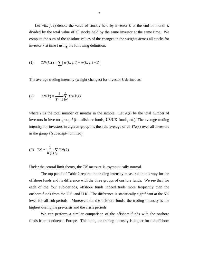
Let w(k, j, t) denote the value of stock j held by investor k at the end of month t,
divided by the total value of all stocks held by the same investor at the same time. We
compute the sum of the absolute values of the changes in the weights across all stocks for
investor k at time t using the following definition:
(1) |)1,,(),,(|),( −−= ∑ tjkwtjkwtkTNj
The average trading intensity (weight changes) for investor k defined as:
(2) ∑=−
=T
t
tkTNT
kTN2
),(1
1)(
where T is the total number of months in the sample. Let K(i) be the total number of
investors in investor group i (i = offshore funds, US/UK funds, etc). The average trading
intensity for investors in a given group i is then the average of all TN(k) over all investors
in the group i (subscript-i omitted):
(3) ∑=k
kTNiK
TN )()(
1
Under the central limit theory, the TN measure is asymptotically normal.
The top panel of Table 2 reports the trading intensity measured in this way for the
offshore funds and its difference with the three groups of onshore funds. We see that, for
each of the four sub-periods, offshore funds indeed trade more frequently than the
onshore funds from the U.S. and U.K. The difference is statistically significant at the 5%
level for all sub-periods. Moreover, for the offshore funds, the trading intensity is the
highest during the pre-crisis and the crisis periods.
We can perform a similar comparison of the offshore funds with the onshore
funds from continental Europe. This time, the trading intensity is higher for the offshore
8
funds in three out of four periods, but the difference is statistically significant only in one
period.
The comparison with the funds from Hong Kong and Singapore is interesting. In
each of the four sub-periods, there is no statistically significant difference between the
two groups. Together, this suggests that the more intense trading by the offshore funds
(relative to the U.S. and European funds) that we observe probably comes from the
waiver of capital gains tax that their funds enjoy, rather than the laxity of regulation.
Future research is needed to confirm this conjecture.
The definition of trading intensity has an unattractive feature: if the prices of the
different stocks fluctuate by a different amount, the value of intensity index changes even
if no trading takes place. As a robustness check, we also implement a different definition
of trading intensity in terms of changing weights in the physical shares of stocks. To be
more precise, we let w(k, j, t) be the number of stock j held by investor k at the end of
month t, divided by the total number of shares of all stocks that she held at the same time.
Then, TN(k) and TN are defined in the same way as before. The results are reported in
the lower panel of Table 2. We can see clearly that all the qualitative results from the
previous measure remain to be true here. Thus, the offshore funds do trade more
frequently than onshore funds (especially compared with those from the U.S. and U.K.)
both before the crisis, and even more so during the crisis.
4. Positive Feedback Trading
There are concerns that offshore funds may engage in positive-feedback trading
more aggressively than onshore funds, and that positive feedback trading could
destabilize the market. A positive-feedback-trading pattern is when one buys securities
when the prices rise and sells when the prices fall. This trading pattern can result from
extrapolative expectations about prices from stop-loss orders --automatically selling
when the price falls below a certain point, from forced liquidations when an investor is
unable to meet her margin calls, or from a portfolio insurance investment strategy which
calls for selling a stock when the price falls and buying it when the price rises.
Positive feedback trading can destabilize the market by moving asset prices away
from the fundamentals. Friedman (1953) and many other economists believe that
9
positive feedback traders cannot be important in market equilibrium as they are likely to
lose money on average. However, De Long, Shleifer, Summers, and Waldmann (1990)
argued that in the presence of noise traders, even rational investors may want to engage in
positive feedback trading, and in the process destabilize the market.
Empirical examination of this issue has emerged recently. Using quarterly data
on U.S. pension funds in the U.S. market, Lakonishok, Shleifer, and Vishny (1992, LSV
for short in later reference) did not find strong evidence of significant feedback trading.
On the other hand, and Grinblatt, Titman and Wermers (1995) did find evidence of
positive feedback trading with their sample of 274 U.S. mutual funds during 1975-1984.
Using transaction-level data, Choe, Kho, and Stulz (1999) also find evidence that foreign
investors as a group engage in positive feedback trading in Korea. No paper that we are
aware of compares the positive trading tendencies of offshore versus onshore trading
strategies.
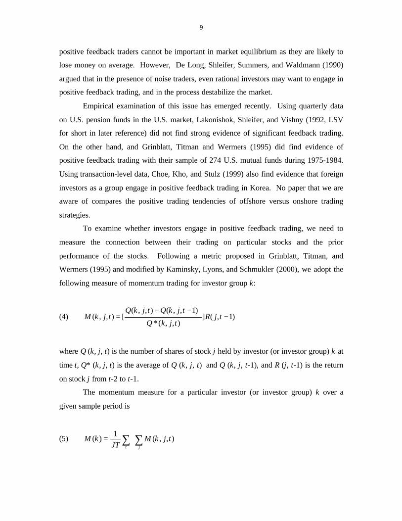
To examine whether investors engage in positive feedback trading, we need to
measure the connection between their trading on particular stocks and the prior
performance of the stocks. Following a metric proposed in Grinblatt, Titman, and
Wermers (1995) and modified by Kaminsky, Lyons, and Schmukler (2000), we adopt the
following measure of momentum trading for investor group k:
(4) )1,(]),,(*
)1,,(),,([),,( −
−−= tjR
tjkQ
tjkQtjkQtjkM
where Q (k, j, t) is the number of shares of stock j held by investor (or investor group) k at
time t, Q* (k, j, t) is the average of Q (k, j, t) and Q (k, j, t-1), and R (j, t-1) is the return
on stock j from t-2 to t-1.
The momentum measure for a particular investor (or investor group) k over a
given sample period is
(5) ∑∑=jt
tjkMJT
kM ),,(1
)(
10
where J is the total number of stocks traded by k, and T is the total number of time
periods under consideration.
Under the null of no feedback trading (in either direction), the mean value of M
(k) is zero. Furthermore, M (k) is asymptotically normal (as J and T approach infinity).
If there is systematic positive feedback trading, then M (k) would be positive. On the
other hand, if there is systematic negative feedback trading, then M (k) would be
negative.5
To avoid possible biases in quantifying the trading behavior, we exclude certain
observations (investors or stock-month). First, investors who declare their purpose of the
stock purchase as direct investment are excluded because they do not engage in active
trading. Second, stocks not owned by any foreign investor in the previous month are
excluded. Since short-selling is not permitted, any change in position in these stocks can
only be a buy by foreigners. Third, stocks that have reached foreign ownership limit are
dropped because any change in the net position of the foreign investors as a whole has to
be a sell to Korean investors. The last two criteria are meant to minimize possible biases
in computed momentum.
Table 3 reports the basic finding on momentum trading. For the first three sub-
periods including the crisis episode, there is no statistically significant evidence that the
offshore funds engage in either positive or negative feedback trading. The exception is
the recovery phrase when they engage in contrarian trading.
The U.S./UK funds make an interesting comparison. Their momentum trading
statistics are always significantly different from zero in all sub-periods. While they may
engage in contrarian trading in the pre-crisis and recovery stages, it is precisely during
the crisis when they adopt a “buy-high-sell-low” positive-feedback-trading pattern. Their
tendency to engage in the positive feedback trading strategy during the crisis is
significantly greater than the offshore funds at the five- percent level.
The momentum statistics for the funds from continental Europe are very similar to
their counterparts from the U.S. and U.K. In particular, while they may engage in
5 Our data does not allow us to examine a portfolio rebalancing effect. Portfolio rebalancing normally callsfor selling appreciating stocks and buying depreciating stocks, the opposite of positive feedback trading.So the presence of a portfolio rebalancing effect would imply that positive feedback trading may bestronger than our statistic suggests (but negative feedback trading may be weaker).
11
contrarian trading in non-crisis periods, they pursue positive feedback trading strategy
during the crisis.
The funds from Hong Kong and Singapore display a weaker tendency to engage
in momentum trading. However, they do engage in positive feedback trading during the
crisis, which is similar to the funds from the U.S. and Europe, but different from the
offshore funds.
To summarize, to the extent that positive feedback trading may be destabilizing in
the emerging markets, the offshore funds in our sample are unique in our sample by not
engaging in it. All three control groups demonstrate a statistically significant tendency to
engage in positive feedback trading during the crisis (though contrarian trading during
some other times).
In Table 3, the returns on the stocks are measured in units of the local currency,
the won. Since the investors in the sample are all international, maybe a more relevant
measure of the return should be based on the U.S. dollar, which allows the impact of the
exchange rate movement to be taken into account. We have also re-computed the
statistics of the momentum trading by using the U.S.-dollar returns (not reported to save
space). While the numerical values of the statistics vary from those in Table 3, the
qualitative features are very similar. Most important, we find that the funds in all the
three control groups engage in positive feedback trading during the crisis, but the
offshore funds are an exception to this pattern.6
A possible defense of positive feedback trading is that foreign investors (residing
abroad) may be informationally disadvantaged relative to domestic investors. They may
take a (relatively greater) decline in the price of a particular stock as unfavorable news
revealed by domestic investors, and may therefore rationally choose to sell it (more
aggressively relative to other stocks) (See Brennan and Cao, 1997, for such a model). It
may be useful to check if the positive-feedback-trading pattern in our sample is ex post
profitable. We do it in two steps. First, in each month, we form an equally-weighted
portfolio of the ten best performing stocks, and another equally-weighted portfolio of the
6 We have re-done the momentum trading calculations for the full sample (i.e. without excluding theobservations discussed in this section). The difference in momentum trading between the offshore andonshore funds becomes statistically insignificant in all sub-periods and for all pair-wise comparisons.
12
ten worst performing stocks, based on the previous month’s return defined in won. The
results are reported in Table 4.
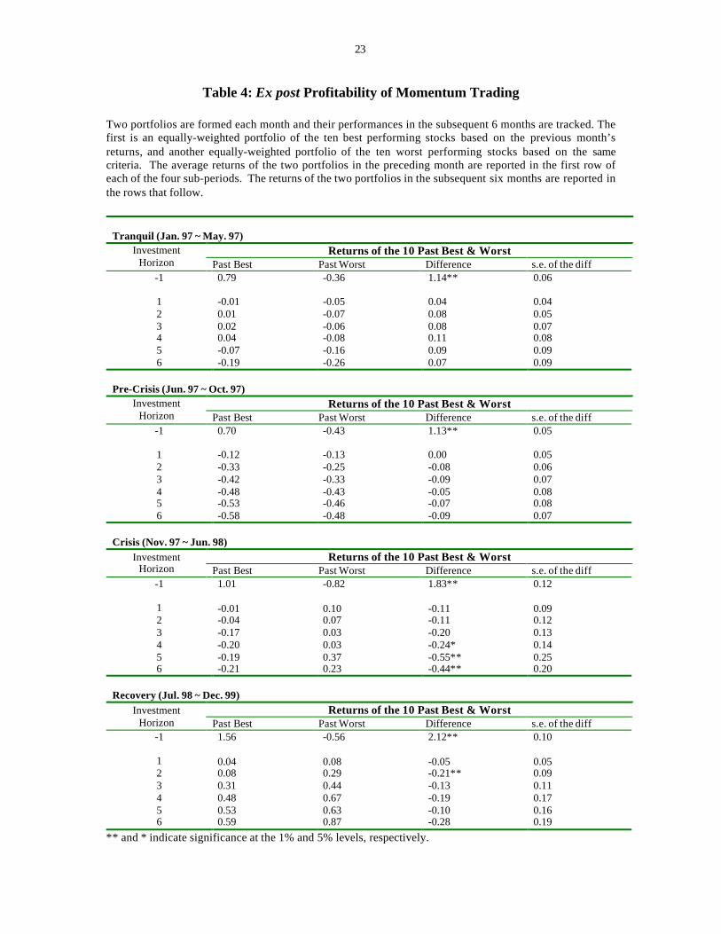
The average returns of the two portfolios in the previous months are reported in
the first row of each of the four panels (representing the four different sub-periods) in
Table 4 (labeled as “horizon -1”). Second, we track their performances over the
subsequent six months. The results are reported in the other rows of Table 4 (labeled as
“horizons 1-6”). We perform a difference in mean test (mean return of the past winners
minus that of the past losers).
During the tranquil or pre-crisis period, there is no significant difference between
the past winners and past losers in terms of their subsequent returns. However, during
the crisis (as well as the recovery) stages, the relative ranking of the winners and losers
reverses itself: on average, past winners tend to do worse than past losers in terms of the
subsequent returns. This is true at all horizons from one to six months. The difference in
performance is significant statistically at horizons over 4 months during the crisis. In
other words, if one has to choose between a positive and a negative feedback trading
strategy during this sub-period, the negative feedback strategy would have done better.
As a robustness check, we also form equally weighted portfolios of the 30 best
performing and the 30 worst performing (based on previous-month’s returns) stocks (not
reported to save space). For these enlarged portfolios, again, there is reversal in the
ranking of relative performance during the crisis. A contrarian trading strategy rather
than a positive feedback one would have been more profitable for this sub-period.
As qualifications, we note that our thought experiments above have not adjusted
for risk levels of the stocks, and do not preclude the possibility that a positive feedback
trading strategy could be profitable within a day or for horizons longer than six months.
We make an attempt to compare the “risk-adjusted” performance of the positive and
negative feedback trading strategies as actually pursued by some funds in our sample. We
focus on the group of the U.S. and U.K. funds, as they are the largest group. Using a
technique proposed by Grinblatt and Titman (1993), we adjust for risk by comparing the
returns of the new and the old portfolios of the investor. In other words, the risk levels on
the new and the old portfolios are assumed to be similar so that the return on the new
portfolio in excess of the old is naturally adjusted for its risk level.
13
We proceed in two steps. First, we classify all the investor-month pairs into two
categories, positive versus negative feedback traders, depending on whether an investor’s
momentum measure, M, is positive or negative in a given month. Second, for each
category, we compute the following risk-adjusted returns, averaged over all traders in the
same group.
(6) ),(]),,(*
)1,,(),,([
1)( ntjR
tjkQtjkQtjkQ
KJTnePerformanc
tjk
+−−= ∑∑∑
where K, J, and T are number of investors in the group, number of stocks, and number of
months in the period, respectively. Lower case “n” in “Performance(n)” and R(j, t+n)
denotes “return horizon.” For example, R(j, t+1) and R(j, t+3) are the returns for stock j
over 1-month and 3-month horizons respectively. Under the assumption that that the
systematic risks for the old and new portfolios are (approximately) the same,
“Performance(1)” and “Performance(3)”measure the risk-adjusted return for the new
portfolio over one and three month horizons, respectively.7
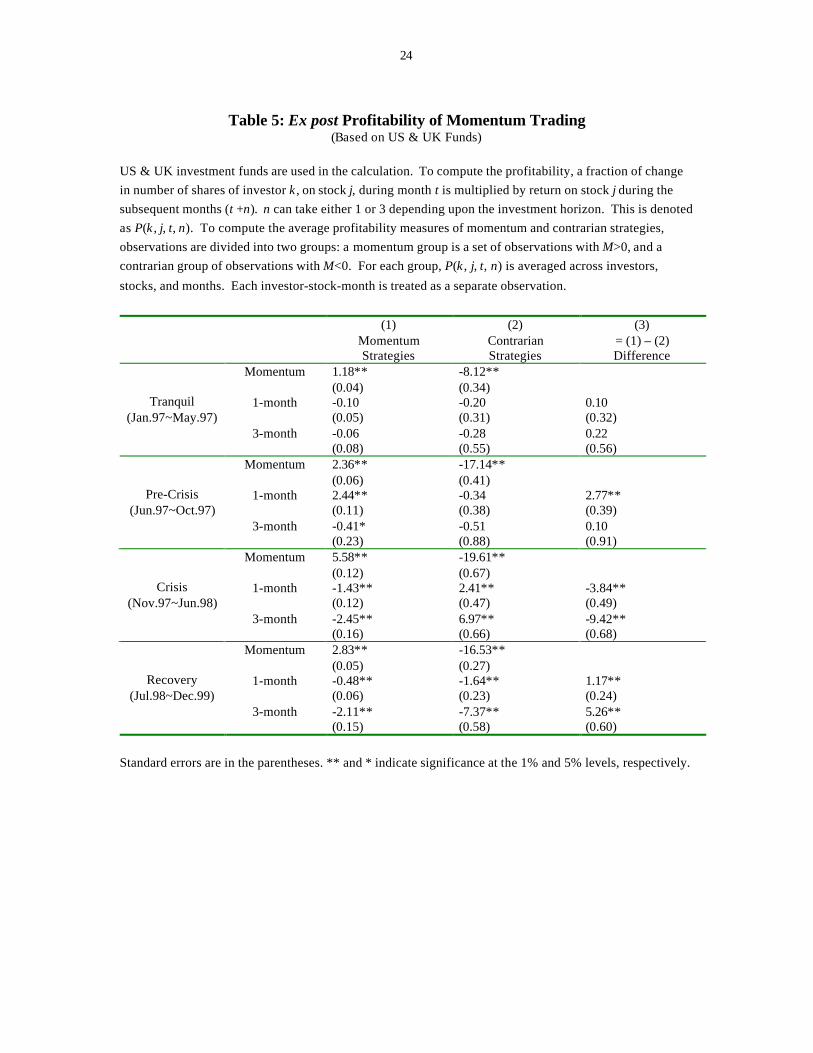
Table 5 reports the profitability calculations for the two trading strategies. Using
this new definition of ex post profitability, the positive feedback trading looks less
terrible. In particular, it appears to do better than a contrarian strategy before the crisis
(at the one-month horizon) and during the recovery period. However, it is precisely
during the crisis, during which most funds were engaging in positive feedback trading,
when such a strategy turns out to be unprofitable. To summarize, on the basis of the
implied ex post profitability (without adjusting for risk), a contrarian strategy seems to
dominate a positive feedback strategy. On the basis of a risk-adjusted measure of
profitability, the positive feedback strategy looks better, though continues to be inferior to
a contrarian strategy during the crisis episode.
4. Herding
7 Grinblatt and Titman (1993) provide some evidence that the betas are the same for the two portfolios intheir sample.
14
Herding is the tendency that investors of a particular group mimic each other’s
trading. Portfolio investors may herd rationally or irrationally. Informational asymmetry
may cause uninformed but rational speculators to choose to trade in the same way as
informed traders (Bikhchandani, Hirshleifer and Welch, 1992; and Banerjee, 1992).
Since the informational problem may be more serious when it comes to investing in a
foreign market than the domestic one, herding may also be more severe. Whether
offshore funds herd more or less than the onshore funds depends on their relative capacity
in collecting and processing information about the emerging market in question.
There is an alternative explanation for herding among institutional investors.
Unlike individual investors, fund managers face regular reviews (e.g., quarterly for
mutual funds, and annually for pension funds) on their performance relative to a
benchmark and/or to each other. This may induce them to mimic each other’s trading to
a greater extent than they otherwise would (See Scharfstein and Stein, 1990). By this
logic, whether the offshore funds herd more or less than the onshore funds depends on
whether informational asymmetry is greater or less for them. By this logic, there might
be less herding among offshore funds if they are subject to either fewer or less frequent
performance reviews.
There have been several empirical papers that quantify herding behavior, starting
with Lakonishok, Shleifer, and Vishny (or LSV, 1992), followed by Grinblatt, Titman,
and Wermers (1995), and Wylie (1997), and Choe, Kho, and Stulz (1999). None of these
papers compares different herding tendencies by different investor types on data from a
single source, which we do here.
We employ the herding index measure proposed by LSV (1992). While we refer
to the LSV measure as a herding index as they do, it is useful to remember that what it
measures is the correlation in trading patterns among members of a group (the tendency
to which investors buy or sell the same subset of stocks). Obviously, herding leads to
correlated trading, but the reverse may not be true.
Let ),,( tjiB be the number of investors in group i that have increased the
holdings of stock j in month t (i.e., number of net buyers), and ),,( tjiS the number of
investors in group i that have decreased the holdings of stock j in month t (number of
net sellers). Let ),( tip be the number of net buyers in group i aggregated across all
15
stocks in month t divided by the total number of active traders (number of net buyers
plus number of net sellers) in group i aggregated across all stocks in month .t Then,
),,( tjiH is defined as the herding index for investors in group i, on stock ,j in month .t
(7) ),(),,(),,(
),,(),(
),,(),,(),,(
),,( tiptjiStjiB
tjiBEtip
tjiStjiBtjiB
tjiH −+
−−+
=
(8)
∑∑
∑
==
=
+= N
j
N
j
N
j
tjiStjiB
tjiBtip
11
1
),,(),,(
),,(
),(
(9) ∑=
=N
j
tjiHN
tiH1
),,(1
),(
(10) ∑∑= =
=T
t
N
j
tjiHNT
iH1 1
),,(1
)(
H(i, t) is the herding index for group i in month t, averaged across all stocks. H(i)
is the herding index for group i, averaged across all months in the sample. In the
definition of H(i, j, t), ),( tip is subtracted to make sure that the resulting index is
insensitive to general market conditions (i.e., a bull or bear market). By taking absolute
values, the first term in equation (7) captures how much of the investment is polarized in
the direction of either buying or selling. The second term in equation (7), also called as
adjustment factor, is subtracted to correct for the mean value of the first term under the
assumption of no herding. The second term can be computed under the assumption that
),,( tjiB follows a binomial distribution. Note that for large N and T, ),( tiH and )(iH
follow normal distributions by the central limit theorem.
To avoid any possible bias in computing the herding indices, we exclude certain
investors and observations (stock-month) from our sample. Similar to the sample we
have constructed to examine positive feedback trading, we exclude here (1) direct
investors, (2) stock-months for which the foreign ownership limit is reached, and (3)
stock-months for which the stocks are not owned by foreign investors in the previous
month. The last exclusion is motivated by the short-selling constraint. When short
16
selling is not allowed, any trade on that stock would have to first show up as a buy, thus
biasing the herding index upward (Wylie, 1997). Finally, if a stock in a given month is
traded by only one foreign investor in that group, that observation is dropped.
The basic results are presented in Table 6. For offshore funds in each sample
period, we report the corresponding herding statistics, H(i), with standard errors in the
parenthesis below. Then we perform a sequence of difference-in-mean tests between
offshore and onshore funds. The most important findings are the following. First, for
both offshore funds as well as the three groups of onshore funds, there is clear evidence
of herding: the herding measure is statistically different from zero for all funds in each
sub-period, except for the Hong Kong/Singapore funds in the pre-crisis episode. Second
and most importantly, the evidence suggests that, to the extent that there is a difference in
the herding tendency, the U.S./U.K. funds herd significantly more than their offshore
counterparts in two of the four sub-periods (and are comparable with the offshore funds
in the other two sub-periods). The offshore funds do herd statistically significantly more
than the European onshore funds during the crisis episode. But this does not generalize
to other sub-periods or to comparisons with other onshore funds. We have re-done the
same calculations for the whole sample (rather than the restricted sample reported in
Table 6). Broadly similar results are obtained (not reported to save space). One notable
exception is that, in the full sample, the offshore funds no longer herd more during the
crisis sub-period than the European onshore funds.
Collectively, the evidence rejects the presumption that offshore funds would
generally herd more aggressively than their onshore counterparts. If anything, there is a
bit of evidence that the U.S. and U.K. onshore funds can sometimes herd significantly
more than the offshore funds.
So far, we have seen evidence that investment funds do engage in herding, though
offshore funds do not necessarily do so more than their onshore counterparts. It may be
useful to investigate whether herding has actually been profitable for the funds at least on
an ex post basis.
Let R(j, t, n) denote the return of stock j from t to t+n (in won). Let H(k, t) denote
LSV herding index for stock j in month t . For each investor group, we run the following
Table 2: Trading Intensity(Frequency of change in portfolio weights)
Panel A Weighted by Value
Sub-Periods
(1)Offshore Centers
(2)Excess Trading
overUS &UK
(3)Excess Trading
overContinental Europe
(4)Excess Trading
overHK & Singapore
Tranquil(Jan.97~May.97)
0.17**(0.02)
0.05**(0.02)
0.02(0.02)
0.03(0.03)
Pre-Crisis(Jun.97~Oct.97)
0.21**(0.02)
0.05**(0.02)
0.08**(0.02)
0.03(0.03)
Crisis(Nov.97~Jun.98)
0.21**(0.02)
0.04**(0.02)
-0.03(0.03)
-0.01(0.03)
Recovery(Jul.98~Dec.99)
0.17**(0.01)
0.03**(0.01)
0.001(0.02)
-0.02(0.02)
Panel B Weighted by Number of Shares
Sub-Periods
(5)Offshore Centers
(6)Excess Trading
overUS &UK
(7)Excess Trading
overContinental Europe
(8)Excess Trading
overHK & Singapore
Tranquil 0.16**(0.03)
0.05*(0.03)
0.03(0.03)
0.02(0.04)
Pre-Crisis 0.20**(0.03)
0.05*(0.03)
0.09**(0.03)
0.03(0.04)
Crisis 0.22**(0.02)
0.06**(0.02)
0.002(0.03)
0.004(0.04)
Recovery 0.17**(0.01)
0.02*(0.01)
0.02(0.02)
0.01(0.02)
Standard errors are in the parentheses. ** and * indicate significance at the 1% and 5% levels, respectively.
22
Table 3: Momentum Trading
Sub-Periods
(1)Offshore Centers
(2)Excess Trading
overUS &UK
(3)Excess Trading
overContinental Europe
(4)Excess Trading
overHK & Singapore
Tranquil(Jan.97~May.97)
0.69(0.50)
0.15(0.53)
0.54(0.55)
0.94(0.96)
Pre-Crisis(Jun.97~Oct.97)
0.11(1.47)
0.71(1.50)
3.95*(2.16)
0.08(1.70)
Crisis(Nov.97~Jun.98)
1.66(3.04)
-6.51**(3.13)
-3.71**(3.37)
-3.66(3.68)
Recovery(Jul.98~Dec.99)
-4.93**(1.96)
-4.12**(1.99)
-1.71(2.48)
-3.63(2.80)
Standard errors are in the parentheses. ** and * indicate significance at the 1% and 5% levels, respectively.
23
Table 4: Ex post Profitability of Momentum Trading
Two portfolios are formed each month and their performances in the subsequent 6 months are tracked. Thefirst is an equally-weighted portfolio of the ten best performing stocks based on the previous month’sreturns, and another equally-weighted portfolio of the ten worst performing stocks based on the samecriteria. The average returns of the two portfolios in the preceding month are reported in the first row ofeach of the four sub-periods. The returns of the two portfolios in the subsequent six months are reported inthe rows that follow.
Tranquil (Jan. 97 ~ May. 97)Returns of the 10 Past Best & WorstInvestment
Horizon Past Best Past Worst Difference s.e. of the diff-1 0.79 -0.36 1.14** 0.06
** and * indicate significance at the 1% and 5% levels, respectively.
24
Table 5: Ex post Profitability of Momentum Trading(Based on US & UK Funds)
US & UK investment funds are used in the calculation. To compute the profitability, a fraction of change
in number of shares of investor k , on stock j, during month t is multiplied by return on stock j during the
subsequent months (t +n). n can take either 1 or 3 depending upon the investment horizon. This is denoted
as P(k , j, t, n). To compute the average profitability measures of momentum and contrarian strategies,
observations are divided into two groups: a momentum group is a set of observations with M>0, and a
contrarian group of observations with M<0. For each group, P(k , j, t, n) is averaged across investors,
stocks, and months. Each investor-stock-month is treated as a separate observation.
(1)MomentumStrategies
(2)ContrarianStrategies
(3)= (1) – (2)Difference
Momentum 1.18**(0.04)
-8.12**(0.34)
1-month -0.10(0.05)
-0.20(0.31)
0.10(0.32)
Tranquil(Jan.97~May.97)
3-month -0.06(0.08)
-0.28(0.55)
0.22(0.56)
Momentum 2.36**(0.06)
-17.14**(0.41)
1-month 2.44**(0.11)
-0.34(0.38)
2.77**(0.39)
Pre-Crisis(Jun.97~Oct.97)
3-month -0.41*(0.23)
-0.51(0.88)
0.10(0.91)
Momentum 5.58**(0.12)
-19.61**(0.67)
1-month -1.43**(0.12)
2.41**(0.47)
-3.84**(0.49)
Crisis(Nov.97~Jun.98)
3-month -2.45**(0.16)
6.97**(0.66)
-9.42**(0.68)
Momentum 2.83**(0.05)
-16.53**(0.27)
1-month -0.48**(0.06)
-1.64**(0.23)
1.17**(0.24)
Recovery(Jul.98~Dec.99)
3-month -2.11**(0.15)
-7.37**(0.58)
5.26**(0.60)
Standard errors are in the parentheses. ** and * indicate significance at the 1% and 5% levels, respectively.
25
Table 6: Herding
Sub-Periods
(1)Offshore Centers
(2)Excess Trading
overUS &UK
(3)Excess Trading
overContinental Europe
(4)Excess Trading
overHK & Singapore
Tranquil(Jan.97~May.97)
4.09**(0.88)
-2.34**(1.01)
1.02(1.26)
1.62(1.25)
Pre-Crisis(Jun.97~Oct.97)
5.15**(1.24)
0.80(1.33)
1.19(1.55)
3.39*(1.97)
Crisis(Nov.97~Jun.98)
5.85**(1.28)
1.82(1.39)
2.75*(1.62)
-1.90(2.14)
Recovery(Jul.98~Dec.99)
4.51**(0.51)
-2.75**(0.62)
0.18(0.80)
-1.66*(0.86)
Standard errors are in the parentheses. ** and * indicate significance at the 1% and 5% levels, respectively.
26
Table 7: Ex post Profitability of Herding
A sequence of regressions are reported in the table, each with a specification of the following form:
R (j, t, n) = α + stock dummies + time dummies + β1 D (j, t) H (j, t) + β2 [1 - D (j, t)] H (j, t) where R (j, t,n), is the ex post return of stock j from month t to t + n. H (j, t ) is the herding on stock j at time t. D (j, t)and 1-D (j, t ) are dummies for herd-to-buy and herd-to-sell, respectively. Standard errors and numbers of
observations are in parentheses and squared brackets, respectively.
One-month HorizonHerd-Buy
β1
Herd-Sellβ2
R2
[# obs.]Offshore -0.06 -0.10 0.60
(0.15) (0.10) [93]US-UK 0.03 -0.03 0.38
(0.07) (0.04) [633]Continental Europe -0.02 0.09 0.47
(0.10) (0.09) [147]HK-Singapore -0.06 -0.25 0.80
Tranquil
(0.27) (0.26) [29]Offshore -0.14 0.08 0.54
(0.12) (0.14) [176]US-UK -0.12** 0.16** 0.64
(0.06) (0.06) [980]Continental Europe -0.07 -0.08 0.60
(0.14) (0.13) [250]HK-Singapore 0.26 0.23 0.66
Pre-Crisis
(0.34) (0.23) [75]Offshore -0.30* 0.12 0.68
(0.16) (0.12) [203]US-UK -0.06 0.05 0.63
(0.07) (0.06) [1099]Continental Europe 0.11 -0.07 0.74
(0.18) (0.16) [256]HK-Singapore 0.57** 0.01 0.67
Crisis
(0.24) (0.16) [108]Offshore 0.01 0.05 0.41
(0.10) (0.06) [854]US-UK 0.005 0.06 0.38
(0.06) (0.05) [2315]Continental Europe -0.002 0.06 0.40
(0.08) (0.06) [692]HK-Singapore 0.054 -0.01 0.43
Recovery
(0.09) (0.07) [599]
27
References
Banerjee, Abhijit (1992), “A Simple Model of Herd Behavior.” Quarterly Journal of
Economics 107, pp. 797-817.
Bekaert, Greet, and Campbell Harvey, 1998, “Capital Flows and the Behavior of
Emerging Market Equity Returns,” NBER Working Paper No. 6669 (1998)
Bikhchandani, Sushil, David Hirshleifer, and Ivo Welch (1992), “A Theory of Fads,
Fashion, Custom, and Cultural Change as Information Cascades.” Journal of
Political Economy 100, pp. 992-1020.
Brennan, M. J. and H. Cao, 1997, “International Portfolio Investment Flows,” Journal
of Finance 52: 1851-1880.
Brown, Stephen J., William N. Goetzmann, and Roger G. Ibbotson, 1999, “Offshore
Hedge Funds: Survival and Performance, 1989-1995,” Journal of Business, 72(1),
January.
Brown, Stephen J., William N. Goetzmann, and James Park, 1999, “Hedge Funds and the
Asian Currency Crisis of 1997,” forthcoming, Journal of Portfolio Management.
Choe, Hyuk, Bong-Chan Kho, and Rene M. Stulz, 1999, "Do Foreign Investors
Destabilize Stock Markets? The Korean Experience in 1997," Journal of
Financial Economics 54: 227-64.
De Long, J. Bradford, Andrei Shleifer, Lawrence H. Summers, and Robert J. Waldmann
(1990), “Positive Feedback Investment Strategies and Destabilizing Rational
Journal of Finance, Vol. 45, No. 2, pp. 379-395.
Financial Stability Forum, 2000, Report of the Working Group on Offshore Centres,
www.fsforum.org.
Financial Supervisory Service (Korea), 2000, Foreign Investors Trend of 1999.
Frankel, Jeffrey A. and Sergio L. Schmukler (1996), “Country Fund Discounts,
Asymmetric Information and the Mexican Crisis of 1994: Did Local Residents
Turn Pessimistic Before International Investors?” NBER Working Paper No.
5714.
Frankel, Jeffrey A. and Sergio L. Schmukler (1998), “Country Funds and Asymmetric
Information.” Policy Research Working Paper No. 1886, The World Bank.
28
Friedman, Milton (1953), “The Case for Flexible Exchange Rates,” in Milton Friedman,
ed. Essays in Positive Economics (University of Chicago Press, Chicago, IL).
Froot, Kenneth A., Paul G.J. O'Connell, and Mark S. Seasholes, 1998, "The Portfolio
Flows of International Investors I." NBER Working Paper No. 6687.
Forthcoming,
Journal of Financial Economics.
Fung, William, and David A. Hsieh, 1997, “Empirical Characterization of Dynamic
Trading Strategies: The Case of Hedge Funds,” Review of Financial Studies, 10:
275-302.
Goldfajn, Ilan, and Rodrigo Valdes, 1997, “Capital Flows and Twin Crises: The Role of
Liquidity,” IMF Working Paper WP/97/87.
Grinblatt, Mark, and Sheridan Titman, 1993, “Performance Measurement without
Benchmarks: An Examination of Mutual Fund Returns,” Journal of Business, 66:
47-68.
Grinblatt, Mark, Sheridan Titman, and Russ Wermers,1995, “Momentum Investment
Strategies, Portfolio Performance, and Herding: A Study of Mutual Fund
Behavior.” American Economic Review Vol. 85, pp. 1088-1105.
Helm, Robert W., 1997, “Offshore Investment Funds,” Chapter 17 in Clifford E. Kirsch,
ed., The Financial Services Revolution: Understanding the Changing Role of
Banks, Mutual Funds, and Insurance Companies, Chicago, London and
Singapore: Irwin, 1997.
Henry, Peter, 2000, “Stock Market Liberalization, Economic Reform, and Emerging
Journal of Finance 55: 529-564.
Kaminsky, Graciela, Richard Lyons, and Sergio Schmukler, 2000, “Managers, Investors,
and Crises: Mutual Fund Strategies in Emerging Markets,” NBER Working
Paper 7855 and the World Bank Working Paper 2399.
Kim, Woochan, and Shang-Jin Wei, 1999, “Foreign Portfolio Investors Before and
During a Crisis,” NBER Working Paper 6968, February. [Also released as OECD
Economics Department Working Paper No. 210, February, 1999.] Forthcoming,
Journal of International Economics.
Lakonishok, Josef, Andrei Shleifer, and Robert Vishny (1992), “The Impact of
29
Institutional Trading on Stock Prices.” Journal of Financial Economics Vol.32,
pp. 23-43.
Milroy, Robert, 1998, Standard & Poor’s Micropal Guide to Offshore Investment Funds
– 1998-99 Edition. International Offshore Publications Limited, Guernsey,
Channel Islands.
Scharfstein, David S. and Jeremy C. Stein (1990), “Herd Behavior and Investment.”
American Economic Review 80, pp.465-479.
Sharpe, William, 1995, “The Styles and Performances of Large Seasoned U.S. Mutual
Funds, 1985-1994,” Working paper, Stanford University Business School.
World Economic Forum (1998), The Global Competitiveness Report 1998. Geneva:
Switzerland, 1988
Wermers, Russ, 1999, “Mutual Fund Herding and the Impact on Stock Prices,” Journal
of Finance 54: 581-623.
Wylie, Samuel (1997), “Tests of the Accuracy of Measures of Herding.” Unpublished