Page 1
1
Date: February 12, 2018 (updated)
To: John Mathews, Ohio EPA
From: Jay Dorsey and Ryan Winston, Ohio State University Stormwater Management Program
Re: WQv Analysis
Summary
The primary goal of this analysis was to identify the water quality capture volume (WQv) that would
ensure Ohio post‐construction stormwater management practices remove 80 percent of the average
annual total suspended solids (TSS) load from stormwater runoff. The WQv is calculated, on a unit area
basis, as the product of a rainfall event depth and a volumetric runoff coefficient (Rv) that converts the
rainfall depth to runoff. An evaluation of both the WQv event precipitation depth and volumetric runoff
coefficient was necessary to determine the combination of those two inputs that result in 80% TSS
reduction for climatic conditions in Ohio. Based on our evaluation, we recommend that Ohio EPA:
utilize the linear relationship between Rv and impervious area; and
increase the WQv precipitation event depth to 0.90 inches.
Introduction
The State of Ohio acknowledged the importance of managing runoff from small, frequent storm events
when it established prescriptive post‐construction runoff management criteria in the 2003 NPDES
Construction Stormwater General Permit (CGP; Ohio EPA, 2003). According to Ohio EPA the intent of
post‐construction best management practices (BMPs) was “to assure that storm water runoff from
developed land does not negatively impact receiving streams, either through hydrologic impacts or
pollutant discharges” (Ohio EPA, 2007).
Ohio EPA outlined in the Post‐Construction Q & A Document (Ohio EPA, 2007) the process used to
identify a “maximized capture volume” for Ohio that resulted in selection of a 0.75‐inch rainfall depth
for the water quality volume (or WQv) storm event in the 2003 CGP. The WQv is “the amount of
stormwater runoff from a given storm that should be captured and treated in order to remove a
majority of stormwater pollutants on an average annual basis” which is defined as removal of at least
80% of the average annual total suspended solids (TSS) load (Ohio EPA, 2007).
In preparation for the 2018 renewal of the NPDES Construction Stormwater General Permit (CGP), Ohio
EPA revisited the current post‐construction stormwater management criteria (Ohio EPA, 2013) to verify
whether meeting those criteria resulted in attainment of established stormwater management goals.
The analysis consisted of the following activities:
(1) An evaluation of volumetric runoff coefficient;
(2) An analysis of historic precipitation data to develop depth‐frequency relationships for weather
stations representing different climatic regions of Ohio;
Page 2
2
(3) For the same weather stations, quantification of (unrouted) percent volume captured based on
WQv event depth;
(4) Development of Storm Water Management Model (SWMM) version 5.1.012 (US EPA
https://www.epa.gov/water‐research/storm‐water‐management‐model‐swmm) models and
continuous simulation using representative historic precipitation data to predict percent routed
stormwater runoff volume captured for a representative BMP under current (P = 0.75 inches, Rv =
0.0858i3 ‐ 0.78i2 + 0.774i + 0.04) post‐construction WQv criteria.
(5) Development of SWMM models and continuous simulation using representative historic
precipitation data to quantify routed stormwater runoff percent volume captured for four
stormwater BMPs (dry extended detention basin, wet extended detention basin, permeable
pavement, and bioretention) sized for WQv precipitation depths of 0.75, 0.85, 0.90 and 1.00 inches.
(6) Results from activities (4) and (5) above were combined to compare percent routed stormwater
runoff volume captured for a representative BMP under current (P = 0.75 inches, Rv = 0.0858i3 ‐
0.78i2 + 0.774i + 0.04) and proposed (P = 0.90 inches, Rv = 0.05 + 0.009*I) criteria.
VOLUMETRIC RUNOFF COEFFICIENT EVALUATION
Purpose
A volumetric runoff coefficient (Rv) that converts rainfall depth to a stormwater runoff treatment
volume is needed to size post‐construction stormwater management practices. The purpose of this
technical analysis is to evaluate the current method for calculating the volumetric runoff coefficient in
the Ohio NPDES Construction Stormwater General Permit (CGP; Ohio EPA, 2013) against other methods
for determining Rv.
Background
Research in environmental hydrology has highlighted the importance of managing small, frequent
storms (the approximately 98% of events less than 2” rainfall depth) for both water quality and receiving
channel stability (WEF, 1998; Pitt, 1999; NRC, 2009). Small storm hydrology is a widely used method for
the estimation of stormwater runoff volume from rainfall events with depths (i.e., 0.25 – 1.5 inches)
typical of groundwater recharge, volume reduction or water quality treatment requirements
(CALTRANS, 2015). A primary reason for the use of small storm hydrology is that the curve number
method commonly used for estimating runoff from small urban watersheds (NRCS, 1986) is not
intended to be used for small rainfall events (Hawkins et al., 1985; Claytor and Schueler, 1996). Small
storm hydrology can be expressed (CALTRANS, 2015):
Vrunoff = Rv*P*A Equation 1
Where:
Vrunoff = volume of runoff
Rv = volumetric runoff coefficient
Page 3
3
P = rainfall depth
A = drainage area
The volumetric runoff coefficient (Rv) is an empirically derived value that indicates the fraction of rainfall
converted into runoff for that land use (Pitt, 1987; Schueler, 1987). The two most common ways Rv is
determined are (Claytor and Schueler, 1996; CALTRANS, 2015): (1) from an equation in which Rv is a
function of the impervious area within the contributing drainage area; or (2) from look‐up tables in
which Rv is a function of both land use/cover and rainfall depth.
Rv as Function of Impervious Area
The most common small storm hydrology method for predicting runoff volume establishes a linear
relationship between Rv and site imperviousness (Schueler, 1987; Claytor and Schueler, 1996;
CALTRANS, 2015) in the form:
Rv = 0.05 + 0.009*I Equation 2
Where:
I = site imperviousness (%)
This relationship was the best fit linear regression of volumetric runoff coefficient versus watershed
imperviousness (r2 = 0.71) from two years of data collected at 44 monitored development sites with
varied percentages of impervious area (Figure 1; Schueler, 1987). This relationship plots mean runoff
coefficient values against imperviousness, and thus reflects the average rate of rainfall conversion to
runoff over a full range of rainfall depths. The data came primarily from the Nationwide Urban Runoff
Program (NURP), the first nationally‐coordinated effort to understand urban runoff quantity and quality
(USEPA, 1983).
Equation 2 is used by a number of states and municipalities to estimate runoff volume for smaller
storms (CALTRANS, 2015), and has been used in the Simple Method water quality model for estimating
pollutants load since that model’s introduction by Schueler (1987). Other linear relationships between
Rv and site imperviousness have been proposed but are used less widely (CALTRANS, 2015).
Page 4
4
Figure 1. Relationship between volumetric runoff coefficient (Rv) and watershed imperviousness (I). (Schueler, 1987)
Urbonas et al. (1989, 1990), also using the NURP data, found a best‐fit relationship between volumetric
runoff coefficient and watershed imperviousness (r2 = 0.72) using a third‐order polynomial equation
(Figure 2):
Rv = 0.0858i3 ‐ 0.78i2 + 0.774i + 0.04 Equation 3
Where:
i = impervious fraction of the development site
Figure 2. Volumetric runoff coefficient as a function of imperviousness (Urbonas, et al., 1989).
Page 5
5
Equation 3 was included in the WEF manual of practice Urban Runoff Quality Management (WEF/ASCE,
1998) but has found limited use among regulatory authorities (CALTRANS, 2015).
Current Ohio NPDES Post‐construction Approach
The volumetric runoff coefficient Rv (denoted as C in the current CGP; Ohio EPA, 2013) can be
determined one of two ways: (1) by calculating Rv using Equation 3; or (2) by looking up the value for a
particular land use in CGP Table 1 (Figure 3). A comparison of Rv values derived from Table 1, Equation
2 and Equation 3 is shown in Figure 4. Though we are unsure how they were derived, Table 1 values
closely track Equation 2.
Figure 3. Volumetric runoff coefficient by land use (Ohio EPA, 2013)
Figure 4. Rv as determined by Equation 2, Equation 3 and CGP Table 1.
Page 6
6
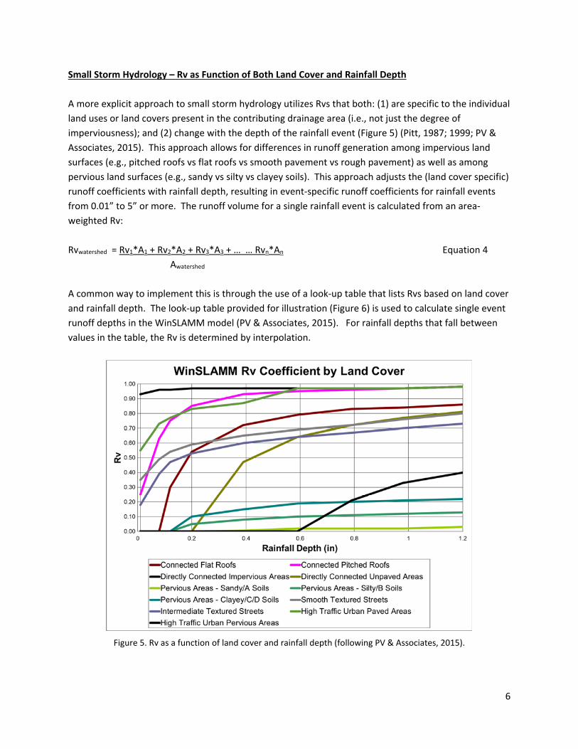
Small Storm Hydrology – Rv as Function of Both Land Cover and Rainfall Depth
A more explicit approach to small storm hydrology utilizes Rvs that both: (1) are specific to the individual
land uses or land covers present in the contributing drainage area (i.e., not just the degree of
imperviousness); and (2) change with the depth of the rainfall event (Figure 5) (Pitt, 1987; 1999; PV &
Associates, 2015). This approach allows for differences in runoff generation among impervious land
surfaces (e.g., pitched roofs vs flat roofs vs smooth pavement vs rough pavement) as well as among
pervious land surfaces (e.g., sandy vs silty vs clayey soils). This approach adjusts the (land cover specific)
runoff coefficients with rainfall depth, resulting in event‐specific runoff coefficients for rainfall events
from 0.01” to 5” or more. The runoff volume for a single rainfall event is calculated from an area‐
weighted Rv:
Rvwatershed = Rv1*A1 + Rv2*A2 + Rv3*A3 + … … Rvn*An Equation 4
Awatershed
A common way to implement this is through the use of a look‐up table that lists Rvs based on land cover
and rainfall depth. The look‐up table provided for illustration (Figure 6) is used to calculate single event
runoff depths in the WinSLAMM model (PV & Associates, 2015). For rainfall depths that fall between
values in the table, the Rv is determined by interpolation.
Figure 5. Rv as a function of land cover and rainfall depth (following PV & Associates, 2015).
Page 7
7
Figure 6. Lookup table for Rv based on land use and rainfall depth (PV & Associates, 2015).
Mixed Approach
Several states and municipalities have expanded on the simple linear relationship to provide some level
of specificity or flexibility where it supports program goals, for example in the implementation of a
runoff volume reduction program (Hirschman et al., 2008; Battiata, 2010; CWP, 2012; VDEQ, 2016). In
such cases, all impervious areas are typically assigned a single Rv value (e.g., Rv = 0.95) for the target
rainfall event depth, whereas pervious areas may have varied Rv values that reflect soil type and/or soil
management (Figure 7).
Figure 7. Soil specific runoff coefficients (Battiata et al., 2010).
Discussion
Both the third‐order regression Rv equation currently used by Ohio (Equation 3 above; Ohio EPA, 2013)
and the linear relationship Rv = 0.05 + 0.009*I (Equation 2 above) are based on the relationship between
runoff volume and impervious area developed from the NURP data (USEPA, 1983). The coefficient of
determination (r2) for the more complicated third‐order regression equation was 0.72 compared to an r2
of 0.71 for the linear (first‐order regression) equation. In its review, CALTRANS (2015) theorized Rv may
not be a linear function of imperviousness, and that the greater slope in the third‐order equation at
higher percent imperviousness (>75%) may reflect that excess runoff at high imperviousness
Page 8
8
“overwhelms” the infiltration capacity of pervious areas. However, the similarity of the coefficients of
determination suggests neither regression model is superior to the other.
The direct, linear relationship between Rv and imperviousness has several practical benefits including
simplicity in communication and calculation. This may explain why most states that have a water quality
treatment volume requirement (similar to Ohio’s WQv) base their calculation of treatment volume
either on the linear equation for Rv (Equation 2; e.g., AK, CT, DC, IA, MD, MN, NC, NH, NY, VA, VT, WV)
or simply by assigning an Rv of 1.0 to impervious areas (e.g., MA, RI) (CALTRANS, 2015; USEPA, 2016).
CALTRANS (2015) noted most municipal design manuals they reviewed also used Equation 2. Ohio and
California (CASQA, 2003) appear to be the only states that use Equation 3. Denver’s Urban Drainage and
Flood Control District (UDFCD, 2010) uses a third order regression equation based on Equation 3, as
does Texas Commission on Environmental Quality for protection of the Edwards Aquifer (TCEQ, 2005).
The most compelling reasons for considering the use of Equation 2 instead of Equation 3 are: (1)
simplicity in applying to redevelopment (i.e., previously developed) sites; and (2) compatibility with
Runoff Reduction Method implementation (Battiata, 2010). Equation 2 equates to an assignment of Rv
= 0.95 to all impervious surfaces and Rv = 0.05 for all pervious areas. This facilitates the use of a simple
WQv relationship for redevelopment sites using Rv as a function of pre‐project (existing) and post‐
project impervious area. Also from this basis, it is simple to keep Rv = 0.95 for impervious areas but
expand the menu of pervious area Rvs to better reflect both soil type (HSG) and/or soil management
(e.g., preserved vs disturbed vs compost amended; forested area vs managed turf) (Figure 7).
The approach used by Washington D.C. assigns a Rv value of zero (0.0) to “natural cover”, a Rv value of
0.25 to “compacted cover” and Rv = 0.95 for impervious area. A similar approach adopted by Ohio
would appropriately credit the relatively high hydrologic function maintained by preserved soils or
recovered by amending soils, and acknowledge the reduced hydrologic function of typical development
site soil degradation.
Rv = [Anat‐am*(Rvnat‐am) + Agraded*(Rvgraded) + Aimp*(Rvimp)] / Atotal Equation 5
Arguments against switching:
People are used to the current “C” equation. Switching will only confuse things.
Switching will increase the WQv treatment volume requirement by an average of 34%
(minimum 6%, maximum 47%) (Figure 4, Table 1).
Arguments for switching:
The linear Rv equation correlates the data as well as the more complicated equation but is
simpler to understand and use. Widespread adoption of the simpler formula and lack of
adoption of the third‐order regression show the more complicated equation holds little appeal
beyond those who developed it.
Page 9
9
Table 1. Comparison in WQv when Rv calculated by Equation 2 and Equation 3 (PWQv = 0.75 in).
The linear correlation between imperviousness and runoff volume lends itself to a simple
accounting method based on site (or drainage area) imperviousness. This will prove useful for
both redevelopment site WQv accounting and Runoff Reduction Method accounting.
One potential benefit would be more straightforward, logical assignment of volumetric runoff
coefficients to land covers other than impervious area, including different hydrologic soil groups
and/or preserved soil, amended soil or compacted soil.
The median 34% increase (range 7% to 48%) in WQv treatment volume is part of the total
adjustment to the WQv necessary ‐ either through modification of the volumetric runoff
coefficient or an adjustment to the WQv rainfall event depth ‐ to achieve 80% TSS removal.
Conclusions/Recommendations
We see no advantage to using Equation 3, whereas Equation 2 is compatible with the assignment of Rvs
for planned Runoff Reduction Method implementation. The negligible improvement in correlation from
Equation 2 to Equation 3 seems to reflect an academic exercise rather than any verifiable improvement
in predicting runoff based on imperviousness. In addition, the direct, linear relationship between Rv and
imperviousness has several practical benefits including simplicity in communication and calculation.
We recommend, at minimum, Ohio EPA switch to volumetric runoff coefficients (Rv) based on the linear
relationship between runoff volume and impervious area. We further recommend Ohio EPA consider
the establishment of differentiated Rv values for better quality (preserved or compost‐amended) soils
and graded (compacted) soils to appropriately credit and incentivize protection or restoration of soil
function.
SLU ‐ Standard Land Use Imp% Rv = fn (i3)
(Eq3)
WQv
ft3/Ac
Rv = 0.05 + 0.009*I (Eq2)
WQv
ft3/Ac
Increase WQv %
Urban Open Space 5 0.08 209 0.09 259 24
Urban Parks 10 0.11 301 0.14 381 27
Low Density Residential 20 0.17 464 0.23 626 35
Med Density Residential 35 0.25 686 0.36 994 45
High Density Residential 50 0.34 924 0.50 1361 47
Multi‐Family Residential 60 0.41 1113 0.59 1606 44
Office Park 75 0.54 1480 0.72 1973 33
Commercial Strip Mall 90 0.73 1988 0.86 2341 18
Page 10
10
WATER QUALITY VOLUME PRECIPITATION DEPTH EVALUATION
Background
Removal of 80% of total suspended solids (TSS) from average annual runoff is a non‐point source water
quality standard established by US EPA (US EPA, 1993, 2005) and adopted by Ohio EPA as a primary
metric of post‐construction stormwater BMP performance (Ohio EPA, 2007). The 90th percentile event
depth has been suggested as a method to determine the runoff volume that should be managed to
meet the water quality treatment performance standard (Claytor and Schueler, 1996; Schueler et al.,
2007; MDEQ, 2014), whereas US EPA (2009) recommended capture of the 95th percentile event for
construction of new federal facilities. Both approaches exclude from the analysis rainfall events with
depth of 0.10 inches or less as “non‐runoff producing events.”
During discussions with Ohio EPA Stormwater staff, we concluded that percent runoff volume captured
by the WQv BMP was a more accurate metric of runoff treated than the 90th percentile rain event depth.
We made an assumption that thoughtful designs of the better‐performing BMPs (wet extended
detention basin, wetland extended detention basin, permeable pavement and bioretention) were
capable of 90% TSS removal for runoff that does not bypass the BMP’s treatment mechanism (extended
detention, filtration, infiltration, etc.) resulting in 80% TSS removal if we could capture 90% of the
annual runoff volume. Therefore, in addition to identifying the 90th percentile rain event depth, we
evaluated the precipitation data to identify the rainfall depth that resulted in capture of 90% of the
annual runoff volume without routing through the stormwater management practice. We then
employed the US EPA’s Storm Water Management Model (SWMM) as described below to estimate the
routed capture volume.
Approach – Precipitation Analysis
We based our precipitation analysis on historic data from a geographically distributed set of Ohio,
Kentucky, and West Virginia‐based weather stations. Our initial target was to analyze between 15 and
20 historic precipitation data sets that represented both the geographic and climatic diversity in Ohio.
An approach to assuring geographic diversity was to attempt to have one or more data sets from each of
the ten (10) isohyetal regions (Figure 8) identified by Huff and Angel (1992) in the Rainfall Frequency
Atlas of the Midwest.
Our initial criteria for acceptance of a precipitation data set were (1) a minimum 30‐year period of
record, preferably the most current 30 years; (2) a reasonable temporal scale (<=1‐hour rainfall data),
(3) 0.01‐inch rain gage recording precision and (4) clean, quality data (few questionable or missing
periods of record). All data sets utilized in the analysis were downloaded from NOAA’s National Climatic
Data Center (NCDC).
We began by evaluating precipitation data sets for the weather stations managed by the National
Weather Service (NWS) at seven (7) Ohio airports (Akron‐Canton, Cleveland, Columbus, Dayton,
Page 11
11
Mansfield, Toledo, Youngstown), plus two (2) stations located just across the state border at
Huntington, WV and the Cincinnati‐Northern Kentucky (NKI) airport (Figure 9). All these weather
stations met our criteria.
Figure 8. Isohyetal regions for Ohio (Huff and Angel, 1992)
Figure 9. Location of rainfall gages used in analysis.
We also downloaded, reviewed and evaluated the historic precipitation data from over 40 cooperator
weather stations concentrated in geographic areas (primarily south, east and southeast Ohio; NW Ohio
between Dayton, Columbus, and Toledo; and north central between Cleveland and Toledo) in‐between
the airports. No cooperator station data sets met our criteria because of: (1) substantial periods of bad
Page 12
12
or missing data; and (2) a switch in recording hourly precipitation depth from hundredths (i.e., to the
nearest 0.01 inch) to tenths (i.e., to the nearest 0.10 inch) during the period of record (mostly around
1985‐1986) which eliminated the recording of individual events less than 0.1 inch. The lowering of
recording precision likely combined, in many cases, multiple small (<0.1‐inch) events into a single 0.1‐
inch reading. Based on analysis of the data from such sites and comparison against the NWS data at the
airports, this change in depth reporting has substantial impacts on the precipitation depth‐frequency
relationship, rendering these data unrepresentative of long‐term precipitation patterns. For these
reasons, we have not included precipitation data from any cooperator stations in our analyses.
For the nine airport weather stations, we identified the 50th, 60th, 70th, 75th, 80th, 85th, 90th, 95th, and
100th percentile rainfall depth (i.e., cumulative event depth frequency); and quantified cumulative runoff
volume captured across a range of specified WQv depths. These statistics were developed for the
historic precipitation data sets for all events and with events less than 0.10 inches removed; subsequent
discussion focuses only on the results from analysis with events less than 0.10 inches removed as these
events do not generate measurable runoff (Claytor and Schueler, 1996; US EPA, 2005). Summary
descriptive statistics (lat‐long, period of record, start date, end date, average annual precipitation depth,
average annual number of events >= 0.1 inch, etc.) for each station were collated (Table 2).
Gage Location
Latitude
Longitude
Start Date
End Date
Years of Record
Average Annual Precip (in)
Average Annual Number of Events > 0.1 in
Akron‐Canton Airport 40.917 ‐81.433 8/1/1948 12/31/2013 65.5 36.8 73.1
Cincinnati Airport 39.067 ‐84.672 12/3/1950 12/31/2013 63.1 41.6 71.6
Cleveland Airport 41.406 ‐81.852 8/1/1948 12/31/2013 65.5 37.3 75.7
Columbus Airport 39.983 ‐82.867 8/5/1948 12/31/2013 65.4 38.3 72.3
Dayton Airport 39.906 ‐84.219 8/4/1948 12/31/2013 65.5 37.7 69.2
Huntington WV Airport 38.365 ‐82.555 1/1/1962 12/31/2013 52.0 41.9 75.3
Mansfield Airport 40.817 ‐82.517 12/1/1959 12/31/2013 54.1 39.7 73.6
Toledo Airport 41.587 ‐83.806 8/11/1948 12/31/2013 65.4 32.9 64.8
Youngstown Airport 41.255 ‐80.674 8/8/1948 12/31/2013 65.4 37.5 76.7
Mean 62.4 38.2 72.5
Table 2. Summary descriptive statistics for rain gages used in analysis.
Results and Discussion – Precipitation Analysis
The precipitation data record for the nine NWS‐managed airport weather stations revealed excellent
quality data that met our criteria. Airport weather stations are located in 6 of the 10 Ohio isohyetal
regions identified by Huff and Angel (1992; Figure 8) – Regions 1, 3, 5, 6, 7, and 8 – with Region 10
(southeast Ohio) the biggest geographic area not represented in the airport data (a map of the weather
stations used in this analysis is included as Figure 9). The Cincinnati NKI airport weather station is across
Page 13
13
the Ohio River from Region 8, and the Huntington WV airport weather station is located across the Ohio
River from Region 9. The airport data, in our opinion, nicely bracket the ranges of rainfall distributions
likely to be found in Ohio with the Cincinnati data representing one extreme (higher frequency
occurrence of larger events) and the Huntington data leaning that way, and Youngstown, Akron‐Canton,
and Cleveland representing the other extreme (lower occurrence of larger depth events). Columbus
data tracks very closely to the mean of the 9 airports, with Toledo, Mansfield, and Dayton closer to the
mean than to the extremes.
Table 3 and Figure 10 summarize the cumulative event depth‐frequency distribution (from 50th to 95th
percentile) for Ohio precipitation data. This summary data let us discuss geographic variability, ranges of
depths/volumes for the 50th to 95th percentile events, and where the 0.75‐inch WQv event (the current
Ohio EPA standard) fit within those ranges. The 0.75‐inch WQv depth represents, on average, the 81st
percentile event with a range from the 77th percentile event at the Cincinnati airport to the 83rd
percentile event at Youngstown, well below the 90th percentile storm recommended as the water
quality event by Schueler et al. (2007). The 90th percentile storm event depth for Ohio ranges from 0.98
inches for Youngstown to 1.18 inches for the Cincinnati airport, with a mean of 1.07 inches.
Gage Location
50th Percentile
(in)
75th Percentile
(in)
80th Percentile
(in)
85th Percentile
(in)
90th Percentile
(in)
95th Percentile
(in)
Akron‐Canton Airport 0.32 0.58 0.67 0.81 0.99 1.36
Cincinnati Airport 0.37 0.71 0.82 0.98 1.18 1.64
Cleveland Airport 0.31 0.57 0.67 0.80 1.00 1.33
Columbus Airport 0.34 0.63 0.73 0.87 1.07 1.48
Dayton Airport 0.35 0.65 0.75 0.90 1.12 1.54
Huntington WV Airport 0.35 0.66 0.77 0.93 1.17 1.56
Mansfield Airport 0.33 0.64 0.76 0.90 1.11 1.51
Toledo Airport 0.32 0.61 0.71 0.84 1.02 1.39
Youngstown Airport 0.31 0.58 0.66 0.79 0.98 1.29
Mean 0.33 0.63 0.73 0.87 1.07 1.45
Table 3. Rainfall depth‐frequency distribution (events < 0.1‐in removed).
Page 14
14
Figure 10. Cumulative precipitation event depth‐frequency distribution.
A better predictor of water quality treatment is the percent annual runoff volume captured by the water
quality BMP at a given WQv depth. In our analysis, we quantified the runoff volume captured in two
ways:
1. Unrouted or “instantaneous” capture volume – This “capture volume” was calculated by simply
removing the WQv event depth from each individual storm event in the historic precipitation
record. As an example, all storm events with depths less than or equal to the WQv precipitation
depth would be fully captured, whereas for larger storm events the WQv precipitation depth
would be captured with the remainder considered to have bypassed the treatment mechanism
of a properly designed BMP and therefore not be captured. This analysis likely would result in
very conservative estimates of WQv precipitation depth necessary to capture the 90th percentile
event.
2. Routed capture volume – This “capture volume” was estimated by performing a continuous
simulation for the full period of the 65‐year historic precipitation record for Columbus, Ohio
using SWMM models in which a BMP was sized according to Rainwater and Land Development
manual guidance adjusted for the WQv precipitation depth. That SWMM modeling exercise and
analysis is detailed in the next section of this report.
The results of the unrouted capture volume analysis are summarized in Table 4. These data show that
the 0.75‐inch WQv event depth results in an annual mean unrouted capture volume of 79.5% with a
range from 75.7% (Cincinnati) to 82.8% (Youngstown).
Page 15
15
Gauge Location
0.50‐in (%)
0.75‐in (%)
0.90‐in (%)
1.00‐in (%)
1.10‐in (%)
1.25‐in (%)
1.50‐in (%)
Akron‐Canton Airport 69.0 81.2 85.9 88.2 90.1 92.3 94.9
Cincinnati Airport 62.2 75.7 81.1 83.9 86.3 89.0 92.2
Cleveland Airport 69.4 81.6 86.3 88.7 90.6 92.8 95.3
Columbus Airport 66.6 79.5 84.4 86.9 89.0 91.4 94.4
Dayton Airport 64.9 77.9 82.9 85.5 87.8 90.4 93.6
Huntington WV Airport 64.0 77.1 82.2 84.9 87.2 90.0 93.3
Mansfield Airport 65.4 78.3 83.4 86.1 88.3 91.0 94.1
Toledo Airport 68.5 81.2 86.1 88.6 90.6 93.0 95.6
Youngstown Airport 70.5 82.8 87.3 89.7 91.6 93.7 96.0
Mean 66.7 79.5 84.4 86.9 89.1 91.5 94.4
Table 4. Percent runoff volume captured by WQv depth (unrouted).
The difference in precipitation characteristics between far southern Ohio (as represented by the
Huntington, WV and Cincinnati airport data) and northern Ohio (as represented by the Youngstown,
Akron‐Canton, Cleveland and Toledo data) suggest use of regional WQv depths should be considered.
Some states have designated different regional WQv depths based on substantial differences in regional
rainfall characteristics (e.g., MD, NC). In Ohio, there is a 20% difference between the minimum 90th
percentile event depth (0.98 inches at Youngstown) and the maximum (1.18 inches at the Cincinnati
airport). The mean of 1.07 inches falls roughly midway between these values. If considering a 0.9‐inch
WQv capture depth, the difference in unrouted annual volume capture between the minimum (81.1% at
Cincinnati) to the maximum (87.3% at Youngstown) is about 8 percent. These differences are not as
extreme as some other states (NC) but are similar in magnitude to rainfall regions treated separately in
MD. These differences, and the logistics of managing a post‐construction program with multiple WQv
values, should be weighed against benefits gained by region‐specific requirements.
Approach ‐ SWMM Runoff Modeling Analysis
The US EPA Storm Water Management Model (SWMM) version 5.1.012 (US EPA, 2017; hereafter
referred to as SWMM) was used to quantify the average annual runoff volume captured by water
quality BMPs sized for various WQvs. The goal was to identify which combination of volumetric runoff
coefficient and WQv precipitation depth resulted in capture and treatment of 90% of the average annual
runoff volume through the BMP’s primary treatment mechanism (i.e., flow treated through the
extended detention outlet for water quality basins, through the filter media for bioretention, or through
infiltration for permeable pavement systems). It was assumed that runoff discharging through a BMP’s
overflow structure bypasses its primary treatment mechanism (i.e., extended detention/settling,
filtering or infiltration) and would have significantly lower water quality than treated runoff.
Page 16
16
Model inputs for all SWMM models included:
Hourly precipitation data record for Port Columbus Airport (August 1948 – December 2013)
[Note: Port Columbus Airport statistics closely tracked statewide mean and median values
within the statewide analysis (see Table 3, Table 4, Figure 10), suggesting Port Columbus data
were representative.]
Monthly evaporation was developed from data reported for the OSU University Farm in
Columbus, Ohio (Farnsworth and Thompson, 1982 as reported in Harstine, 1991).
Stormwater BMP inputs were developed following guidance in the Rainwater and Land
Development manual (ODNR, 2006) adjusted for WQv.
Subcatchment, drainage network, storage unit and LID inputs followed standard SWMM
modeling guidance as detailed in Rossman and Huber (2016a, 2016b) and James et al. (2010).
[Note: A sensitivity analysis was conducted to test effect on the BMP capture volume by
changing ‐ within the range of potential values ‐ SWMM model input parameters (e.g.,
subcatchment width, subcatchment slope, dstore‐imperv, dWQv, etc.). The sensitivity analyses
did not identify any parameters that would materially change capture volume performance.]
Modeling pervious areas in SWMM introduces a great deal of uncertainty if the modeler does not have
runoff data to calibrate the model to (sometimes even with calibration data). To minimize uncertainty
related to runoff from pervious areas, two strategies were employed:
(1) where it fit the goals of the modeling exercise, models employed watersheds that were 100
percent impervious; and
(2) rather than modeling pervious area using one of the infiltration options, pervious areas were
modeled as impervious area at a ratio of Aimpervious = 0.05* Apervious, consistent with the volumetric
runoff coefficient assigned pervious area (Rv = 0.05) in Equation 2. For example, for a
hypothetical 4‐acre site with 50% imperviousness, the SWMM subcatchment would be modeled
as Aimpervious‐model = Aimpervious‐actual + (0.05* Apervious) = 2.0 Ac + (0.05*2.0 Ac) = 2.1 Ac.
Two SWMM modeling exercises were conducted. The objective of the first exercise was to quantify the
volume captured across a range of imperviousness using the WQv criteria (PWQv = 0.75 inches; Rv =
0.0858i3 ‐ 0.78i2 + 0.774i + 0.04) in the current CGP (Ohio EPA, 2013) to see how the volume captured
compared to the goal of 90% average annual runoff volume captured. For this exercise, watersheds
with drainage areas that were 20, 40, 50, 60, 80 and 100% impervious were modeled to determine the
percentage of volume captured by dry and wet extended detention basins following design criteria in
the Rainwater and Land Development manual (ODNR, 2006).
The objective of the second exercise was to quantify the PWQv necessary to result in 90% average annual
runoff volume captured. For this exercise, it was assumed Equation 2 would be adopted and the WQv
would be calculated according to Equation 1. Hypothetical 100% impervious watersheds (Rv = 0.05 +
0.009*I = 0.95) were modeled for each of four BMPs (dry extended detention basin, wet extended
detention basin, permeable pavement with infiltration, and bioretention) which had the WQv sized for
each of four different PWQv (0.75, 0.85, 0.90 and 1.00 inches) for a total of sixteen separate modeling
Page 17
17
runs. The modeled watersheds for the extended detention basins were 4 acres whereas the modeled
watersheds for the bioretention and permeable pavement were 1 acre.
Results ‐ SWMM Runoff Modeling Analysis
Using SWMM models to simulate the hydrologic routing of runoff through post‐construction stormwater
BMPs designed for the WQv event gives a more accurate representation of runoff volume “captured”
and treated by the BMP than does a simple statistical analysis of precipitation data (Novotny, 2003). An
advantage of using continuous simulation driven by historic rainfall data is the volume captured reflects
measured rainfall and runoff patterns that account for variability in precipitation depth, duration and
intensity, as well as back‐to‐back runoff events (James, 2005).
Working from the premise that appropriately‐selected, well‐designed BMPs are capable of 90% TSS
removal for runoff that discharges through the BMP’s treatment mechanism (extended detention,
filtering, infiltration, etc.), it was stipulated that capturing 90% of the annual runoff volume would result
in 80% TSS reduction:
Total TSS Reduction = Percent Runoff Volume Captured * Percent TSS Removal from Volume Captured
90% Runoff Volume Captured * 90% TSS Removal = 81% Total TSS Reduction
The estimated average annual routed runoff volume captured by wet and dry extended detention (ED)
basins designed to current Ohio EPA (2013) criteria ranged from 71% at I = 50% (wet ED basin) to 83% at
I = 100% (dry ED basin, Figure 11). When multiplied by the assumed 90% TSS removal efficiency (for wet
ED basin only), the resulting estimated average annual TSS reductions ranges from 64% at I = 50% to
73% at I = 100% (Table 5), well below the goal of 80% TSS removal on an average annual basis.
Figure 11. Average annual runoff capture volume as a function of imperviousness; current CGP post‐construction WQv criteria (Ohio EPA, 2013).
Page 18
18
Imperviousness
(%)
Average Annual Runoff
Capture Volume
%
Estimated TSS Reduction
(Assuming BMP Effectiveness = 90%)
%
20 74.0 66.6
40 70.9 63.8
50 70.9 63.8
60 71.4 64.3
80 75.3 67.8
100 81.1 73.0
Goal 90.0 80.0
Table 5. Average annual runoff capture volume and estimated TSS reduction as a function of imperviousness for wet extended detention basins sized for current CGP post‐construction WQv criteria (Ohio EPA, 2013).
SWMM was used to run a series of simulations of four different post‐construction BMPs to determine
the routed stormwater runoff volume captured when each practice was sized for the WQv with Rv
following Equation 2 for four different PWQv (0.75, 0.85, 0.90 and 1.00 inches). The results of these
sixteen (16) simulations are presented in Table 6. Assuming 90% TSS removal for the captured runoff
volume, model results can be extended to estimated average annual TSS load reduction as a function of
PWQv (Table 7, Figure 12)1.
WQv P Depth
(in)
Dry ED Basin
%
Wet ED Basin
(EDv=0.75*WQv)
%
Permeable
Pavement
%
Bioretention
%
0.75 84.6 82.8 85.8 88.9
0.85 88.1 86.3 87.9 90.6
0.90 89.0 87.7 88.9 91.3
1.00 91.2 89.4 90.5 92.7
Table 6. Average annual percent routed capture volume as a function of PWQv.
[Note: Rv determined by Equation 2.]
1 TSS removal estimates for dry extended detention basins were not included in Table 7 because research suggests the TSS removal efficiency of dry basins is typically 60‐70%, well below the 90% removal efficiency assumed for the more effective BMPs (CWP, 2007; Leisenring et al., 2014). It is recommended that Ohio EPA evaluate TSS removal performance of dry extended detention basins, and explore pretreatment, in‐basin treatment enhancements, and/or increasing the WQv for this practice to bring it in line with other approved options.
Page 19
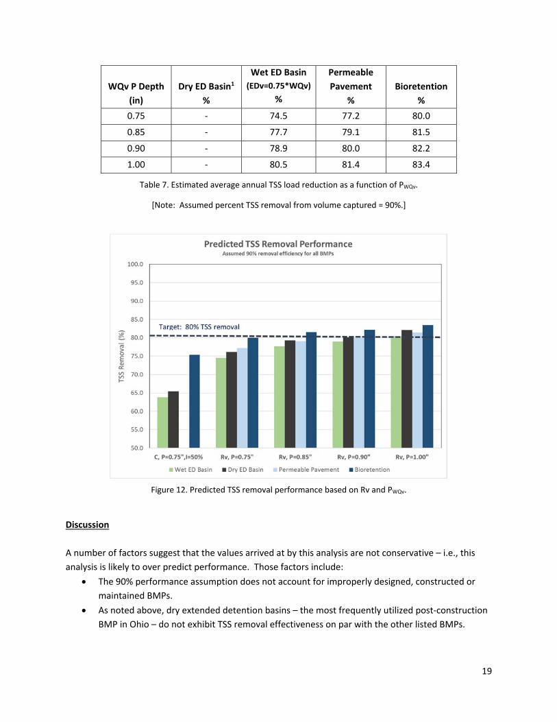
19
WQv P Depth
(in)
Dry ED Basin1
%
Wet ED Basin
(EDv=0.75*WQv)
%
Permeable
Pavement
%
Bioretention
%
0.75 ‐ 74.5 77.2 80.0
0.85 ‐ 77.7 79.1 81.5
0.90 ‐ 78.9 80.0 82.2
1.00 ‐ 80.5 81.4 83.4
Table 7. Estimated average annual TSS load reduction as a function of PWQv.
[Note: Assumed percent TSS removal from volume captured = 90%.]
Figure 12. Predicted TSS removal performance based on Rv and PWQv.
Discussion
A number of factors suggest that the values arrived at by this analysis are not conservative – i.e., this
analysis is likely to over predict performance. Those factors include:
The 90% performance assumption does not account for improperly designed, constructed or
maintained BMPs.
As noted above, dry extended detention basins – the most frequently utilized post‐construction
BMP in Ohio – do not exhibit TSS removal effectiveness on par with the other listed BMPs.
Page 20
20
Soil degradation associated with site development was not taken into account in the SWMM
modeling. The excess runoff associated with soil degradation results in lower capture of runoff
volume, resulting in bypass of more untreated runoff volume and lower TSS removal.
Statewide trends in increased precipitation depth and intensity over time resulted in capture
volume more than 2% lower in the most recent half (1981‐2013) than in the first half (1948‐
1980) of the precipitation record.
Columbus precipitation data was used to estimate volume captured and annual TSS removal
because of its correspondence to statewide averages. Volume captured would be lower, and
TSS removal less, for southern and southwest Ohio due to higher frequency of events greater
than the WQv.
It is recommended that Ohio EPA consider these factors when selecting PWQv.
Conclusions/Recommendations
Ohio EPA has set the threshold for NPDES permit compliance at 80% TSS load removal from post‐
construction stormwater runoff on an average annual basis. This means that a post‐construction
stormwater BMP must (1) control a large enough water quality volume and (2) provide highly effective
TSS removal to remove 80% of the TSS mass (loading) from stormwater runoff. Because a suite of post‐
construction BMPs (wet extended detention basin, wetland extended detention basin, permeable
pavement with or without infiltration, and bioretention) are capable of 90% TSS removal of the volume
treated, a 90% capture volume target was set for average annual stormwater runoff.
The estimated average annual routed runoff volume captured by wet extended basins using current
Ohio EPA post‐construction criteria results in estimated average annual TSS reductions ranges from 64%
to 73%. Similar capture volumes for dry extended detention basins and permeable pavement suggest
current criteria in the CGP do not provide the stated goal of 80% TSS reduction on an average annual
basis, and modifications to the Rv and PWQv should be made.
Based on our evaluation, we recommend the following changes to the post‐construction WQv criteria in
the CGP:
utilize Rv = 0.05 + 0.009*I
increase the WQv precipitation depth (PWQv) to 0.90 inches.
These updates, combined with estimated total suspended solids (TSS) removal efficiencies of 90% for
selected extended detention (wet basin, constructed wetland basin, media filter) and infiltration best
management practices (BMPs) accepted for general use (Table 2; Ohio EPA, 2013), result in removal of
80% of average annual TSS.
Page 21
21
References
Battiata, J., K. Collins, D. Hirschman, and G. Hoffman. 2010. The Runoff Reduction Method. J.
Contemporary Water Research and Education 146: 11‐21.
CALTRANS. 2015. Runoff Coefficient Evaluation for Volumetric BMP Sizing. California Department of
Transportation, Sacramento, CA.
Caraco, D. 2013. Watershed Treatment Model (WTM) ‐ 2013 Documentation. Center for Watershed
Protection, Ellicott City, MD.
CASQA. 2003. Stormwater Best Management Practice Handbook – New Development and
Redevelopment. California Stormwater Quality Association, Menlo Park, CA.
Claytor, R., and T. Schueler. 1996. Design of Stormwater Filtering Systems. Chesapeake Research
Consortium, Inc., Solomons, MD.
CWP. 2007. National Pollutant Removal Performance Database, Version 3. Center for Watershed
Protection, Ellicott City, MD.
CWP. 2012. Stormwater Management Guidebook. Prepared by the Center for Watershed Protection for
Watershed Protection Division, District Dept. of the Environment, District of Columbia.
Farnsworth R. K., and Thompson, E. S., 1982. Mean Monthly, Seasonal, and Annual Pan Evaporation for
the United States, NOAA Technical Report NWS 34 , U.S. Department of Commerce, National Oceanic
and Atmospheric Administration, National Weather Service, 82 pp.
Harstine, L. 1991. Hydrologic Atlas of Ohio. Water Inventory Report No. 28, Ohio Department of Natural
Resources, Columbus.
Hawkins, R., A. Hjelmfelt, and A. Zevenbergen. 1985. Runoff Probability, Storm Depth, and Curve
Numbers. Journal of Irrigation and Drainage Engineering, ASCE 111(4): 330‐340.
Hirschman, D., K. Collins, and T. Schueler. 2008. Technical Memorandum: The Runoff Reduction Method.
Center for Watershed Protection, Ellicott City, MD.
Huff, F.A., and J.R. Angel. 1992. Rainfall Frequency Atlas of the Midwest. Bulletin 71, Illinois State Water
Survey, Champaign, IL.
James, W. 2005. Rules for Responsible Modeling, 4th Edition. Computational Hydraulics International
Press, Guelph, Ontario.
Page 22
22
James, W., L.A. Rossman, and W.R.C. James. 2010. User’s Guide to SWMM 5, 13th Edition. Computational
Hydraulics International Press, Guelph, Ontario.
Leisenring, M., J. Clary, and P. Hobson. 2014. International Stormwater Best Management Practices
(BMP) Database Pollutant Category Statistical Summary Report ‐ Solids, Bacteria, Nutrients, and Metals.
International Stormwater BMP Database (http://bmpdatabase.org).
MDEQ. 2006. 90‐Percent Annual Non‐Exceedance Storms. Internal memo from Dave Fongers to Ralph
Reznick. Michigan Department of Environmental Quality, Lansing.
NCDEQ. 2017. North Carolina Stormwater Control Measure Credit Document (Revised 5‐11‐2017). North
Carolina Department of Environmental Quality, Raleigh.
Novotny, V. 2003. Water Quality: Diffuse Pollution and Watershed Management, 2nd Edition. John Wiley
& Sons, New York.
NRC. 2009. Urban Stormwater Management in the United States. Water Science and Technology Board,
National Research Council. National Academies Press, Washington, DC.
NRCS. 1986. Urban Hydrology for Small Watersheds. Technical Release 55 (TR‐55), Natural Resources
Conservation Service, U.S. Department of Agriculture, Washington, DC.
ODNR. 2006 (with updates). Rainwater and Land Development Manual. Division of Soil and Water
Conservation, Ohio Department of Natural Resources, Columbus.
Ohio EPA. 2003. General Permit Authorization for Storm Water Discharges Associated with Construction
Activity under the National Pollutant Discharge Elimination System. Ohio EPA Permit Number
OHC000002. Ohio Environmental Protection Agency, Columbus.
Ohio EPA. 2007. Post‐Construction Q & A Document (March 2007). Ohio Environmental Protection
Agency, Columbus.
Ohio EPA. 2013. General Permit Authorization for Storm Water Discharges Associated with Construction
Activity under the National Pollutant Discharge Elimination System. Ohio EPA Permit Number
OHC000004. Ohio Environmental Protection Agency, Columbus.
Pitt, R. 1987. Small Storm Urban Flow and Particulate Washoff Contributions to Outfall Discharges. Ph.D.
dissertation, Dept of Civil and Environmental Engineering, University of Wisconsin, Madison.
Pitt, R. 1999. Small Storm Hydrology and Why It Is Important for the Design of Stormwater Control
Practices. In New Applications in Modeling Urban Water Systems, William James (ed.), pp61‐92.
Computational Hydraulics International, Guelph, ON Canada.
Page 23
23
PV & Associates. 2015. WinSLAMM Model Algorithms. PV & Associates, Madison, WI.
Rossman, L. and W. Huber. 2016a. Storm Water Management Model Reference Manual Volume I –
Hydrology (Revised). Office of Research and Development, U.S. Environmental Protection Agency,
Cincinnati, Ohio.
Rossman, L. and W. Huber. 2016b. Storm Water Management Model Reference Manual Volume III –
Water Quality. Office of Research and Development, U.S. Environmental Protection Agency, Cincinnati,
Ohio.
Schueler, T. 1987. Controlling Urban Runoff: A Practical Manual for Planning and Designing Urban BMPs.
Department of Environmental Programs, Metropolitan Washington Council of Governments.
Washington, DC.
Schueler, T., Hirschman, D., Novotney, M., Zielinski, J. 2007. Manual 3: Urban Stormwater Retrofit
Practices Manual. Urban Subwatershed Restoration Manual Series. Center for Watershed Protection,
Ellicott City, MD.
TCEQ. 2005. Complying with the Edwards Aquifer Rules—Technical Guidance on Best Management
Practices. RG‐348 (Revised) with Addendum. Texas Commission on Environmental Quality, Austin, TX.
UDFCD. 2010. Urban Storm Drainage Criteria Manual, Volume 3, Stormwater Quality (updated
November 2015). Urban Drainage and Flood Control District, Denver, Colorado.
Urbonas, B., J.C.Y Guo, and L.S. Tucker. 1989. Sizing a Capture Volume for Stormwater Quality
Enhancement. In Flood Hazard News, Urban Drainage and Flood Control District, Denver, Colorado.
Urbonas, B., J.C.Y Guo, and L.S. Tucker. 1990. Optimization of Stormwater Quality Capture Volume. In
proceedings of Urban Stormwater Quality Enhancement: Source Control, Retrofitting, and Combined
Sewer Technology. American Society of Civil Engineers, New York.
US EPA. 1983. Results of the Nationwide Urban Runoff Program ‐ Final Report. Water Planning Division,
U.S. Environmental Protection Agency, Washington, DC.
US EPA. 1993. Guidance Specifying Management Measures for Sources of Nonpoint Sources of Pollution
in Coastal Waters. EPA 840‐B‐92‐002, Office of Water, U.S. Environmental Protection Agency,
Washington, DC.
US EPA. 2005. National Management Measures to Control Nonpoint Source Pollution from Urban
Areas. EPA 841‐B‐05‐004, Office of Water, US Environmental Protection Agency, Washington, DC.
Page 24
24
US EPA. 2009. Technical Guidance on Implementing the Stormwater Runoff Requirements for Federal
Projects under Section 438 of the Energy Independence and Security Act. EPA 841‐B‐09‐001, Office of
Water, U.S. Environmental Protection Agency, Washington, DC.
US EPA. 2016. Summary of State Post Construction Stormwater Standards (updated July 2016). Office of
Water, U.S Environmental Protection Agency, Washington, DC.
US EPA. Storm Water Management Model (SWMM) v5.1.012. [https://www.epa.gov/water‐
research/storm‐water‐management‐model‐swmm]
VDEQ. Module 4: The Virginia Runoff Reduction Method (current as of June 2016). Virginia Department
of Environmental Quality.
WEF/ASCE. 1998. Urban Runoff Quality Management. WEF Manual of Practice No. 23 and ASCE Manual
and Report on Engineering Practice No. 87. Alexandria, VA and Reston, VA: WEF and ASCE.
WEF/ASCE. 2012. Design of Urban Stormwater Controls. WEF Manual of Practice No. 23 and ASCE
Manual and Report on Engineering Practice No. 87. WEF Press, Alexandria, VA and American Society of
Civil Engineers, Environmental and Water Resources Institute, Reston, VA.