+ All Categories
Home > Documents > OIL AND GREASE IN STORMWATER RUNOFF Michael K. …

OIL AND GREASE IN STORMWATER RUNOFF Michael K. …

Date post: 04-Oct-2021
Category:
Upload: others
View: 1 times
Download: 0 times
Share this document with a friend
252
OIL AND GREASE IN STORMWATER RUNOFF Principal Investigators Michael K . Stenstrom Ph .D . Engineering SystemsDepartment University of California, Los Angeles and GarySilverman Taras A . Bursztynsky, P.E . Association of Bay Area Governments Berkeley, CA 94705 Contributors Anne L . Zarzana Pamela A . Painter Susan E . Solarz RobertScofield Thien-Huong Nguyen Environmental Science and Engineering University of California, Los Angeles 90024 February, 1982 1982 Association of Bay Area Governments
Transcript

OIL AND GREASE IN STORMWATER RUNOFF

Principal Investigators

Michael K. Stenstrom Ph .D .

Engineering Systems DepartmentUniversity of California, Los Angeles

and

Gary Silverman

Taras A. Bursztynsky, P.E .

Association of Bay Area GovernmentsBerkeley, CA 94705

Contributors

Anne L . Zarzana

Pamela A . Painter

Susan E. Solarz

Robert Scofield

Thien-Huong Nguyen

Environmental Science and EngineeringUniversity of California, Los Angeles 90024

February, 1982

• 1982Association of Bay Area Governments

All rights reserved . No part of this training handbook may be reproduced inany form without the permi$sion of the Association of Bay Area Governments .

ABSTRACT

This study, conducted as part of the regional planning mandated by the

Federal Water Pollution Control Act of 1972 (PL92-500), section 208, providesa tool for management of oil and grease runoff from urban areas to the San

Francisco Bay . A field sampling program undertaken to determine the nature

and source of oil and grease . A literature review was performed to evaluateavailable mitigation techniques, and the available techniques were ranked asfavorable, marginally favorable, and unfavorable. Literature reviews were

also conducted to examine previous studies of sources, chemical character-

istics, and environmental fate of oil and grease in urban storm waters, and toexamine potential biological effects of oil and grease inputs on estuarine

envi ronment .

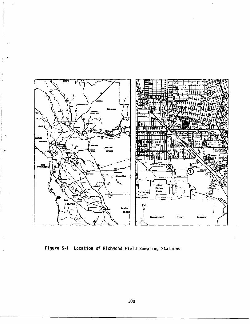
The field sampling program was performed during seven storms in thewinter of 1980-1981 in a watershed in Richmond, Contra Costa County,California . The Richmond watershed was selected for study because it includedindustrial, commercial, residential and undeveloped properties--typical ofmany areas bordering the San Francisco Bay . Oil and grease concentration andrunoff flow rate was determined for samples collected at the mouth of thewatershed and at four other sampling stations, each representative of a landuse type, at regular intervals during each storm . Gas chromatography wasperformed on selected samples to identify chemical characteristics of the oiland grease.

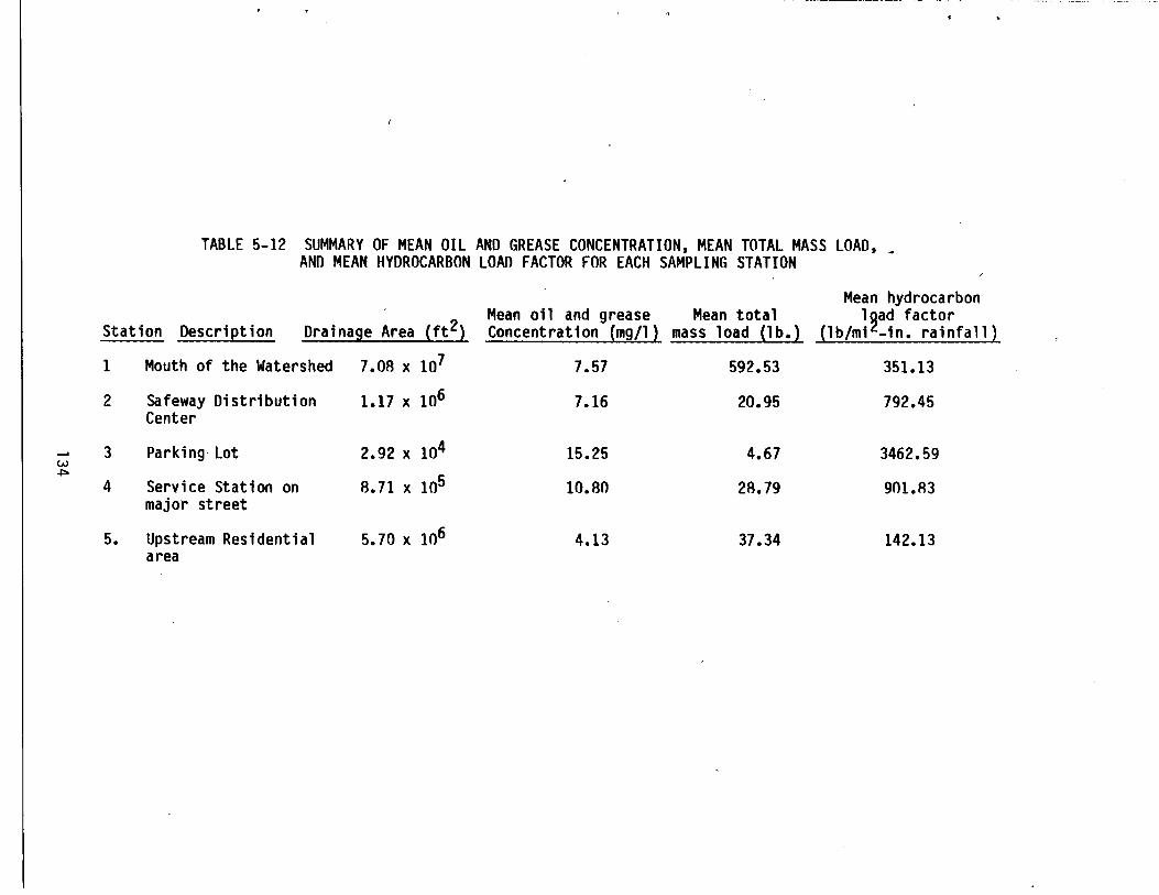
The results of the field sampling program indicate the the oil and greasecontribution to urban storm water runoff is highly dependent upon the land usetype . Mean oil and grease concentration in runoff flow ranged from 4 .13 mg/1(upstream residential area) to 15 .25 mg/l (parking lot) . Another parameter,hydrocarbon load factor, as calculated as an index of comparison of thepotential oil and grease contribution from each land use category underuniform conditions of rainfall . These values ranged from 142 lb ./sq . mi .-in .rainfall (upstream residential area) to 3452 .59 1 ./sq. mi .-in . rainfall(parking lot) . Oil and grease concentration was found to show little rela-tionship to individual storm characteristics such as days between storms, rateof rainfall, or runoff flow rate . However, a moderate "first flush" effectwas observed in this study . Automobile crankcase oil and automobile exhaustparticulates appeared to be important sources of oil and grease in runoffflow, as indicated by gas chromatography analysis of the runoff samples .Evidence of spills was also found in several samples .

Favorable mitigation techniques included non-structural control methodssuch as oil recycling programs and improved automobile emissions control aswell as several structural control measures--porous pavement, green beltsimproved street and parking lot cleaning, biological end-of-pipe systems suchas wetlands or marshes, sorption systems for manholes and gutter entrances,and disperson devices . The applicaton of these mitigation techniques werefound to be highly site specific . Most treatment systems were marginallyfavorable or poor .

iii

Acknowledgements

This work was funded by the Association of Bay Area Governments,

supported in part by a Section 208 grant from the U .S . EPA .

Many individuals and organizations provided valuable assistance to the

study . Dr Peter Russell of ABAG developed the initial analaytical laboratory

program . RAMLT Associates performed the field sampling, including the

development of flow measuring devices, and provided the initial review of

mitigation techniques and the review of hydraulics. Acurex Corporation

analyzed the oil and grease samples . Mr. Robert Fuller of the City of

Richmond Public Works Department was very helpful in selecting appropriate

sampling sites, furnishing equipment and documents and providing insight into

the characteristics of the watershed .

Professor Richard L . Perrine of the UCLA Environmental Science and

Engineering program and Dr . Eugene Leong of the Association of Bay Area

Governments provided advice and help throughout the study . The clerical and

typing assistance of Ms . Karen Shimahara, Ms . Mariko Kitamura and Ms . Ann

Berry are greatly appreciated .

iv

TABLE OF CONTENTS

Page

ABSTRACT iiiACKNOWLEDGEMENTS ivLIST OF FIGURES viiiLIST OF TABLES x

CHAPTER 1 INTRODUCTION 1

CHAPTER 2 OIL AND GREASE IN URBAN STORMWATER RUNOFF :

5ITS CHEMICAL CHARACTERIZATION, POTENTIAL SOURCES,AND ENVIRONMENTAL FATE

Introduction 5Sources and Patterns of Hydrocarbon Pollution 7Chemical Characterization of Urban Stormwater

Runoff Previous Studies 11Transport Mechanisms 33Summary 41

CHAPTER 3 BIOLOGICAL EFFECTS OF OIL AND GREASE 43

Introduction 43Oil Types 43Oil in Urban Runoff 44Oil Toxicity 45Petroleum Hydrocarbons in Water and Sediments 49Effects of Marine Organisms 51Ecological Effects 57

CHAPTER 4 OIL AND GREASE MITIGATION TECHNIQUES 63

Introduction 63Problem Characterization 64Source Control 66

Automotive Oil Control 66Land Use 67

Oil and Grease Removal 68Runoff Treatment 70Review of Treatment Methods 72Existing Practices in the Petroleum Industry 81Centralized Storage 85Decentralized Storage 88Biodegradation 90Outfal1 94No Control 95Summary 96

CHAPTER 5 DATA COLLECTION AND ANALYSIS 97

Objectives 97Site Description 97

v

TABLE OF CONTENTS (continued)

Page

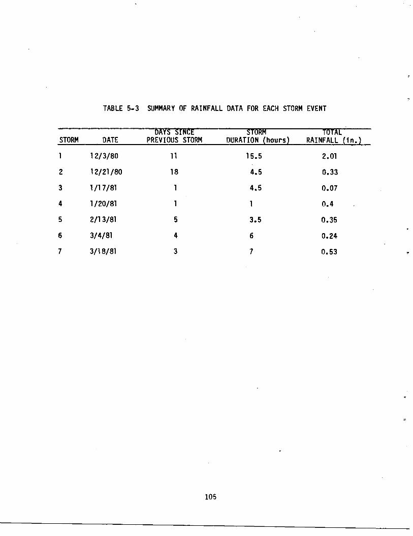
Land-Use and Sample Station Description 101Storm Characterization 104Experimental Design 104Sample Collection Oil and Grease Determination 104Measurement of Oil and Grease Concentration 108Rainfall Measurements 109Flow Measurements 110

Station 1 110Station 2 113Station 3 114Station 4 115Station 5 115

Settlability of Oil and Grease 118Characterization of Oil and Grease in Richmond

Watershed Runoff 120Data Analysis 120Raw Data and Simple Statistics :.122Runoff Flow 122Oil and Grease Concentration and Total Mass Load in Runoff125Hydrocarbon Load Factor 130Summary of Raw Data and Simple Statistics 133Correlation Coefficients 137Linear Regressions 137Analysis of Variance 139Summary of Analysis of Variance and Regressions 144Scatter Diagrams : Examination of First Flush Effect145Comparison of Results to Previous Studies 152Summary of Quantitative Data 157Identification of Oil and Grease by Sedimentation 158Identification of Oil and Grease Compounds inStormwater Samples 159

Comparison to Previous Work - GC Results 167

CHAPTER 6 APPLICATION OF THE ABMAC MODEL TO THERICHMOND WATERSHED ∎ ∎ . . . . ∎1 70

Introduction 170Model Selection 170ABMAC Model 172Calibration of the ABMAC Model for the Richmond Watershed175Model Simulations 182Summary 188

CHAPTER 7 SELECTED CONTROL TECHNIOUES 189

Favorable Non-Structural Techniques 189Oil and Grease Recycling 191Vehicle Inspections and Maintenance Programs 193Identification of Critical Compounds in Oil and Grease194

Favorable Structural Control Techniques 195

vi

TABLE OF CONTENTS (continued)Page

Cleaning of Surface Material 196Porous Pavement 198Oil Sorption Systems 200Greenbelts 201Wetlands 203

Dispersion Devices 205Marginally Favorable Mitigation Techniques 208Unfavorable Control Techniques 210Summary 211

CHAPTER 8 CONCLUSIONS AND RECOMMENDATIONS 214

REFERENCES 218

APPENDICES 229A. Raw Data 229B . Nomenclature 235C. Corrections to the ABMAC Coding 236

vii

LIST OF FIGURESPage

2-1

Hydrograph-pollutograph of October 16, 1974 Storm Event122-2

Mass Loading Rate of Pollutographs of AliphaticHydrocarbons in October 16, 1974, Storm Event 13

2-3

Mass Loading Rate Pollutographs of AromaticHydrocarbons in October 16, 1974, Storm Event 14

2-4

Effect of Amount of Rainfall on Total HydrocarbonsDischarged From Storm Sewer 15

2-5

Gas Chromatograms of Total Hydrocarbon Fractionsin Storm Runoff 19

2-6

Analytical Scheme 232-7

Fingerprint Chromatograms of Aliphatic Hydrocarbons in StormWater Particulates and Used Crankcase Oil by FID26

2-8

Analytical Scheme 272-9

Gas Chromatograms of Aromatic Hydrocarbons Using aFlame Ionization Detector 29

2-10

Gas Chromatograms of Aromatic Hydrocarbons FractionUsing a Flame Photometric Detector-Sulfur Mode 30

2-11

Gas Chromatograms on Apiezon L of Aliphatic Hydrocarbons322-12

Total Dust and Dirt Dry Weight Accumulation 352-13

Accumulation of Pollutions by Land Use 37.2-14

Per Axle Dry Weight Loading vs . Roadway Barrier Height404-1

Typical Porous Asphalt Concrete Parking Lot Pavement714-2

API Oil/Water Separation 764-3

Shell Parallel-Plate Interceptor 774-4

Shell Corrugated Plate Interceptor 784-5

Flow Restrictor/Oil Separator Control Deviceand Catch Basin 89

4-6

TSI Gravity Separator 914-7

Proposed Oil Adsorbent Device for Manhole 925-1

Location of the Richmond Field Sampling Station1005-2

Channel Cross Section for Station 1 1115-3

Typical 90° V-notch Weir 1155-4

Rating Curve for Station-5 1175-5

Typical Rectangular Weir 1195-6

Oil and Grease Concentrations as a Function ofTime for Station 1 148

5-7

Oil and Grease Concentrations as a Function ofTime for Station 2 149

5-8

Oil and Grease Concentrations as a Function ofTime for Storm 5 150

5-9

Normalized Oil and Grease Mass Loading Rates for Storm 31535-10

Normalized Oil and Grease Mass Loading Rates for Storm 41545-11

Normalized Flow Rates for Storm 3 1555-12

Normalized Flow Rates for Storm 4 1565-13

Gas Chromatogram for Storm 1, Station 1, Sample 81625-14

Gas Chromatogram for Storm 6, Station 1, Sample 31635-15

Gas Chromatogram for Storm 6, Station 1, Sample 51645-16

Typical Gas Chromatograms for Refined Products1686-1

Schematic of the ABMAC Model 1747-1

Hypothetical Green Belt for Treatment of Stormwaters2027-2

Hypothetical Diffuser Pumping Facility Schematic Design206

viii

LIST OF FIGURES (continued)

7-3

Hypothetical Diffuser Pumping Facility ProcessFlow Design 207

b

ix

Page

2-1

2-22-32-4

2-53-1

3-2

3-3

4-1

4-2

4-3

4-44-54-65-15-25-35-4

5-5

5-6

5-7

5-8

5-95-10

5-11

5-12

5-13

5-14

5-15

LIST OF TABLES

Page

Budget of Petroleum Hydrocarbons Introducedinto the Oceans 6Estimated Petroleum Pollution, Delaware Estuary 8Measured Values of Hydrocarbon Concentration 9Comparative Gas Chromatographic Results of AliphaticHydrocarbons in Stormwater Particulates and Standard Oils25Grease Accumulation 39Comparative Toxicity of Different Aromatic HydrocarbonsExpressed in 96-hr LC5p 's with Concentration in ppm47Summary of Effects of Petroleum Hydrocarbons on theGrowth and Reproduction of Marine Animals 54Toxicity of Selected Marine Organisms Exposed toPetroleum Hydrocarbons 57Summary of Potential Treatment Techniques forRemoval of Oil from Water 73Oil and Suspended-Solids Removal in Gravity-TypeSeparators ?0Estimated Effluent Quality From Primary Oil/WaterSeparation Processes 80Manufacturers of Gravity Separation Equipment 86Manufacturers of Filtration Equipment 87Manfacturers of Other Oil/Water Separation Equipment87Land Use in the Richmond Watershed 99Description of Sampling Stations 102Summary of Rainfall Data for Each Storm Event 105Mean Runoff Flow at Each Station Associated with

TotalEach

SRunoffv Flow.(100 gal)~for~Each~Storm~at~Each~~~~~~~~~~~" "

∎ 1 23

Sampling Location 124Rate of Runoff to Rainfall : K Values for Each Stationand Storm 126Mean Oil and Grease Concentration at Each StationAssociated with Each Storm Event 127Mean Oil and Grease Concentration (mg/1) Observedat Each Sampling Station 128Flow Weighted Average Concentrations of Oil and Grease129Total Mass Load (TMASS) of Oil and Grease (ib) forEach Storm at Each Sampling Station 131Hydrocarbon Load Factor Defined as Pounds Oil andGrease per Square Mile Drainage Area per Inch Rainfall132Summary of Mean Oil and Grease Concentration, MeanTotal Mass Load, and Mean Hydrocarbon Load Factor forEach Sampling Station 134Summary of the Relationship of Precipation/Runoffto Oil and Grease Concentration and Hydrocarbon Mass Loadfor Each Storm Event 135Correlation Coefficients Between Oil and GreaseLoad Parameters 138Multivariate Regress Analysis : Summary of StrongestRelationships to Oil and Grease Concentration 140

x

5-16

5-17

5-18

5-19

5-205-215-225-21

6-16-26-36-46-56-67-1

LIST OF TABLES (continued)

Analysis of Variance (Randomized Block Design) Test ofthe Hypothesis that Oil and Grease Concentration (OG1) isa Function of the Independent Variables : Station Number is

Page

Treated as a Block 141Analysis of Variance (Randomized Block Design) Testof the Hypothesis that Oil and Grease Mass Load (TMASS)is a Function of the Independent Variables ; Station Numberis Treated as a Block 142Analysis of Variance (Randomized Block Design) Test ofthe Hypothesis that Total Runoff Volume (TFLOW) is aFunction of the Independent Variables ; Station Numberis Treated as a Block 143Linear Regression : Oil and Grease Concentration as aFunction of TimeScatter Diagrams Mass Loading Rate as a Function of Time151Results of Settling Column Tests, Station 1 160Results of Settling Column Tests, Station 3 160Summary of Gas Chromatograms with Respect to RetentionTime 165Station Parameters 177Land Use Parameters 177Model Residuals 183ABMAC Mitigation Simulations - 60% Reduction 184ABMAC Mitigation Simulations - 90% Reduction . . . :185ABMAC Growth Simulations 186Summary of Control Techniques 212

CHAPTER I

INTRODUCTION

One of the most significant sources of pollution to natural waters is

non-point source pollution, . such as pollution from diverse origin such as

contaminated urban storm waters . Storm waters contain a large variety of

contaminants, including oil and grease . Oil and grease has long been recog-

nized as a pollutant which may cause significant environmental damage . To

control non-point source pollution, Public Law 92-500 provided for area-wide

planning in section 208 . The goal of area-wide planning is a systematic way

to provide for treatment plants, regulation of land use, and the overall

control of pollution at minimum costs . This study is in response to the

planning mandated by PL92-500 . The results of this study are intended to

provide a basis for a pilot program of oil and grease control in urban storm-

water in the San Francisco Bay area .

Oil and grease from urban stormwaters represents a low level, chronic

release of oil and grease, as opposed to oil spills . Unfortunately, very

little research has been performed on the environmental effects of low level

discharges . Oil spills are commonly large scale point sources of oil and

grease release which are aesthetically displeasing and obvious sources of

pollution . In contrast to spills, oil and grease in urban runoff may origi-

nate from a myriad of small, non-point sources : vehicle exhaust, crankcase

oils, fuel oils, gas stations, fried chicken stands . There is no obvious

single source of oil and grease runoff pollution and often no visible sign of

this pollution in the runoff . Yet substantial quantities of oil and grease

may be released into the Bay exclusive of spills .

1

To put the hydrocarbon input into the Bay in perspective, one must

examine the major inputs into the Bay . In 1972, a dry water year, total

stormwater runoff into the Bay was approximately 1,110,000 acre-feet, with .

waste effluent roughly 900,000 acre-feet . The outflows from the delta dwarfed

these contributions, consisting of approximately 9,500,000 acre-feet . Delta

outflows and variability of outflow, although presently reduced from historic

level through the use of upstream reservoirs, has ranged from about 4,000,000

acre-feet during the 1931 drought to greater than 50,000,000 acre-feet in

1938 . Tidal action flushes about 6 percent of the Bay volume with each tidal

cycle, and is a major mechanism for Bay pollutant removal (California, State

of, 1979) .

While water quantity derived from runoff and treated effluent comprises

only a relatively small percentage of total Bay effluent, pollutant contribu-

tions from these sources appear very significant . Approximately one-half of

the pollutant sources of BOD, heavy metals, total nitrogen and total phospho-

rus enter the Bay from point sources and surface runoff with a greater

contribution predicted for the future (Russell, et . al ., 1980) ., A similar

comprehensive examination of oil and grease sources into the Bay has not been

performed . However, for comparative purposes, an integrated petroleum refin-

ery the size of the 350,000 bbl/day plant in Richmond could legally discharge

an average of about 500 kg/day of oil and grease/day into the Bay . Using the

East Bay Municipal Utility District's (EBMUD) estimate of about 10 mg/l oil

and grease in their effluent, domestic waste could account for an additional

15,000 kg/day of oil and grease discharged into the Bay . Projecting from the

oil and grease concentrations observed in this study, it is estimated that

stormwater contributes approximately 22,000 kg/day of oil and grease to the

Bay . The effects of stormwater pollution are aggravated because the discharge

of pollutants occur during brief time periods .

2

Runoff normally enters the Bay along the shorelines, often in areas not

subject to rapid dilution or flushing. This is particularly true in the South

Bay, where fresh water flushing is only common during periods of large

storms . An estuarine system like the Bay offers one of the most productive of

all types of habitat, with spawning grounds and nurseries for many kinds of

fish and shellfish, and vital habitats for waterfowl using the Pacific

Flyway . Along the shorelines exist shellfish beds and areas vital to success-

ful fish spawning, feeding and migration. These areas also harbor much of the

vegetative life responsible for the high level of productivity . Microcrus-

taceans and microorganisms providing the necessary link between the primary

producers and many of the larger organisms also exist predominately along the

shorelines . Since it is at the shorelines that most of the runoff enters the

Bay, it is the shoreline that appears most vulnerable to contamination .

Shoreline contamination could result in severe consequences affecting large

areas of the Bay .

Objectives of this study were to determine the potential benefits and

favorable techniques for managing oil and grease in stormwater . It was hoped

that the results of the study would be generally applicable to urban areas, as

opposed to a site-specific result which would only be relevant to the study

area . Therefore the approach was structured to relate the findings to quanti-

tative aspects of the land-use types, storm characteristics, and oil and

grease characteristics .

To accomplish these objectives a 2 .5 square mile watershed in the city of

Richmond, California was selected as the study area . This watershed was

chosen because it included industrial, commercial, undeveloped, and residen-

tial properties, which is typical of many areas bordering San Francisco Bay .

Within the study area, five sampling locations were chosen, and an experi-

3

mental program was designed to analyze urban storm waters for oil and grease

during seven storms in the winter of 1980-1981 . Samples were collected during

storms on a regular basis and were analyzed for oil and grease concentra-

tion. Selected samples were also analyzed using gas chromatography in the

hopes of determining the nature and source of the oil and grease . An analysis

of variance and a regression analysis were applied to the resulting data .

To ascertain the importance of land use pattern on the watershed's total

oil and. grease budget, a simple modeling and simulation study was performed .

Using this model, the effects of potential treatment methods were simulated

for each land use pattern . Growth scenarios were also simulated. Finally,

incorporating the modeling results with the data and the literature review

allowed the development of a set of recommended treatment techniques .

4

CHAPTER 2

OIL AND GREASE IN URBAN STORMWATER RUNOFF : ITS CHEMICAL

CHARACTERIZATION, POTENTIAL SOURCES, AND ENVIRONMENTAL FATE

Introduction

Hydrocarbons enter the marine environment from a number of natural and

man-made sources . As shown in Table 2-1, marine transportation is the largest

single contributor of hydrocarbons to the oceans . Most of these emissions

occur during normal operations, with accidents accounting for only a small

fraction of the total . The contribution of urban runoff is comparable to that

from natural seepage, especially when it is considered that some of the input

from river runoff is the result of upstream urban stormwater runoff . Large

spills of oil cause extensive obvious disruption of the environment . In low

concentrations, hydrocarbons are of interest as pollutants chiefly due to

their toxicity . Point sources of hydrocarbon pollution, such as refineries or

tanker loading terminals, can be and are monitored and regulated rather

easily . Pollution from non-point sources, due to its diffuse nature, is much

more difficult to study and to regulate .

There is a large body of. literature on general non-point source pollution

of urban stormwater runoff (Browne, 1978 ; Browne, 1980 ; Field and Cibik,

1980) . Information on hydrocarbon pollution of these waters is much less

extensive . It is estimated that about 5% of the total hydrocarbons entering

the ocean come from urban stormwater runoff (NAS, 1975) . As contributions

from other sources decrease due to tighter controls and better technology, the

importance of urban stormwater as a hydrocarbon source will increase . As an

example of the increasing importance of urban storm water, estimates of pre-

sent and future contributions of hydrocarbon source will increase . As an

TABLE 2-1 BUDGET OF PETROLEUM HYDROCARBONS INTRODUCED INTO THE OCEANS

a mta, million metric tons annually (N .A .S ., 1975) .

6

Input Rate (mta) aSource Best Estimate Probable Range Reference

Natural seeps 0.6 0.2-1 .0 Wilson et al (1973)

Offshore production 0 .08 0 .08-0.15 Wilson et al (1973)

TransportationLOT tankers 0 .31 0.15-0.4 Results of workshopNon-LOT tankers 0 .77 0 .65-1 .0 panel deliberationsDry docking 0 .25 0.2-0.3Terminal operations 0 .003 0 .0015-0.005Bilges bunkering 0 .5 0 .4-0.7Tanker accidents 0 .2 0.12-0 .25Nontanker accidents 0.1 0.02-0 .15

Coastal refineries 0 .2 0.2-0 .3 Brummage (1973a)

Atmosphere 0.6 0.4-0 .8 Feuerstein (1973)

Coastal municipal wastes 0.3 Storrs (1973)

Coastal, Nonrefining, 0.3 Storrs (1973)industrial wastes

Urban runoff 0.3 0 .1-0.5 Storrs (1973),

River runoff 1 .6

Halihagen (1973)

Storrs (1973),

TOTAL 6.113

Hallhagen (1973)

example of the increasing importance of urban storm estimates of present and

future contributions of hydrocarbons to the Delaware Estuary are presented in

Table 2-2 .

Sources andPatternsofHydrocarbonPollution

Hydrocarbons in urban runoff can come from accidental spills or deliber-

ate dumping of lubricating oils or fuel oils ; from emissions of engines during

normal operation, such as vehicle exhaust particulates or drippings of crank-

case oil ; from dustfall or rainout of atmospheric particulates ; from spilling

of crude or refined petroleum products during production, processing and

transportation ; from leached or eroded pavement ; from natural seepage on land

or erosion of organic bearing sedimentary rocks ; . or from natural biogenic

sources (Eganhouse and Kaplan, 1981h ; Hunter et al, 1979 ; Wakeham, 1977) .

Wakeham (1977) shows that natural hydrocarbons are only a minor contribution

to most urban runoff . Of the other sources, used crankcase oil has been

identified by gas chromatography studies as the most probably major

contributor (Hunter et al, 1979 ; MacKenzie and Hunter, 1979 ; Wakeham, 1977) .

However, vehicular particulate emissions have a similar GC profile so that

differentiating between these two highly probably sources is difficult .

Values for hydrocarbon concentration in urban stormwater as measured by

various investigators are presented in Table 2-3 . As is explained in the

previous section, great care must be taken in comparing these results due to

the diverse experimental and analytical methods used to derive them.

Hydrocarbons associated with storm water runoff have been found to be

predominantly aliphatic . Eganhouse and Kaplan (1981a) measure 88% aliphatics

while Hunter et al (1975, 1979) measure about 70% aliphatics average . Hunter

et al (1979) found aromatics formed 31 .6% of the particulate fraction and only

7

8

TABLE 2-2 ESTIMATED PETROLEUM POLLUTION, DELAWARE ESTUARY(Whipple and Hunter, 1979)

1975 (lb/day) Future lb/da

Spills 6,000 6,000

Municipal Effluent 7,800-15,600 2,000

Refinery Effluent 24,000 1,900

Other Industrial Effluent 8,900 6,200

Urban runoff 10,500 10,700

TOTAL (rounded) 57,000-65,000 26,800

(1) Hunter et al, 19792) Wakeham, 19773) Soderlund and Lehtinen, 1972

(4) Eganhouse and Kaplan, 1981a

TABLE 2-3 MEASURED VALUES OF HYDROCARBON CONCENTRATION

PLACE DESCRIPTIONHYDROCARBONFRACTION

CONCENTRATION (mg/1)High Low Mean

Philadelphia, PA (1) Urban runoff AliphaticParticulates 3 .41 1 .12 2.28Soluble .50 .12 .29

Aromatic-Particulates 1 .65 .49 1 .01Soluble .19 .04 .11

Seattle, Wash . (2) Bridge runoff Aliphatic 24.0 6 .0 12 .0Urban runoff Aliphatic 7 .5 .2 1 .2

tD Bridge runoff Total 96 .0 0.0 27 .0Urban runoff Total 16 .0 1 .0 10 .0Freeway runoff Total 60 .0 10 .0 44.0

Stockhom, Sweden (3)

Los Angeles, CA (4)

Terrace housesSuburbanHighwayMixed

River

TotalTotalTotalTotal

Aliphatic 11 .5Aromatic 1 .6

26 .1% of the soluble fraction . Conversely, Eganhouse and Kaplan (1981a)

report the aliphatic to aromatic ratio to be 11 .5 for particulates and only

2.9 for the dissolved phase, meaning that aromatics are proportionately more

common in the dissolved phase.

Hydrocarbons are consistently found to be predominantly associated with

particulates . Determinations of the average proportion of hydrocarbons found

on particulates are : 81% (Shaheen, 1975), 96 .4% (Hunter et al, 1979) and

greater than 85% (Eganhouse and Kaplan, 1981a) . Eganhouse and Kaplan (1981a)

determined that the most of the hydrocarbons are found on finer particulates

(Shaheen, 1975 ; Sartor et al, 1974) . This could be a surface to volume

effect, smaller particulates having more surface area for adsorption of hydro-

carbons per unit of weight than do larger particulates . It has not been

determined if the hydrocarbon distribution is uniform within any individual

particle size category, nor is the degree of saturation of the particles

known .

Patterns of hydrocarbon pollution vary with watershed and storm charac-

teristics . The effects of watershed topography, size, and shape on runoff

distribution are well known in hydrology . The concentration of hydrocarbons

in urban runoff is a function of the degree of urbanization and types of land

uses in the watershed (Whipple and Hunter, 1979 ; Soderlund and Lehtinen, 1972 ;

Rimer et al, 1978) .

Due to the inherently intermittent nature of storms, runoff waters can

contribute sudden sharp peaks of pollutant to receiving bodies . This shock

loading can increase the effects of pollutants on life forms if the pollutant

concentrations are high during the early part of a storm. These high concen-

trations which fall off quickly are termed the "first flush" . Hunter et al

(1979) suggest that this effect is due to the washing off of easily

10

transported hydrocarbons . Soderlund and Lehtinen (1972) observe no such

effect with suspended solids . The actual pollutant at any time during a storm

appears to be a function of the flow at that time . Figures 2-1 to 2-3 show

this effect (Hunter et al, 1979) . Peaks in flow are matched by peaks in

hydrocarbon load . The correlation coefficient between flow and hydrocarbon

load is quite low, however, indicating that they are not linearly related

(Eganhouse and Kaplan, 1981a)

Hunter et al (1979) found that the total hydrocarbon load for a storm is

a function of the total rainfall during the storm . The particulate fraction

of the load rises exponentially with increase in total rainfall, as shown in

Figure 2-4 . Load cannot continue to increase exponentially indefinitely, and

more data for larger storms are required for further definition of this

function . There is disagreement in the literature as to the importance of the

time period between storms in determining hydrocarbon pollutant levels .

Some sources consider this factor to be important (Huber et al, 1975 ;

Metcalf and Eddy, Inc ., 1971 ; Shaheen, 1975) and others do not (Whipple et al,

1977 ; Hunter et al, 1979) . It is possible that where rainfall patterns are

roughly constant throughout the year the time between storms may not be as

important a parameter as in watersheds with, long dry seasons . The effects of

time period between storms will be discussed further in the section on trans-

port mechanisms .

ChemicalCharacterizationofUrbanStormwater Runoff-PreviousStudies

Very few studies looking at the oil and grease content of urban storm-

water runoff using gas chromatography (GC) or gas chromatography in

combination with mass spectroscopy (GC/MS) have been undertaken to date . The

few studies which have been done have attempted to identify oil and grease

11

10

∎ ∎

0

I0

1000

I

2000

10/16/74 STO R M

HYDROGRAPHIC DATA

Q FLOW - METERS3/SECTOTAL VOLUME 5,946.2 m3

TOTAL HYDROCARBONCONCENTRATION mg/1

II13000

4000

5000

TIME (SEC)

1

6000

i

7000

Figure 2-1 Hydrograph-pollutograph of October 16, 1974, storm event(Hunter et al, 1979)

1 2

08000

1 .4

1 .2

1 .0

8.0

4.0

2.0

10/16/74 STO R M

ALIPHATIC HYDROCARBONS

Q PARTICULATE ALIPHATIC HYDROCARBONSTOTAL LOADING 6.66 Kg

SOLUBLE ALIPHATIC HYDROCARBONSTOTAL LOADING 2.26 Kg

IIIII -"-~I a

I1000

2000

3000

4000

5000

6000

7000

8000TIME (SEC)

Figure 2-2 Mass loading rate pollutograph of aliphatic hydrocarbons inOctober 165, 1974, storm event (Hunter, et . al ., 1979)

13

1 .5

1.0

0.5

0

Y

∎ ∎

0I

I1000 2000

II3000

4000

5000TIME (SEC)

10/16/74 STORM

AROMATIC HYDROCARBONS

∎∎

0 PARTICULATE AROMATIC HYDROCARBONSTOTAL LOADING 2.91 Kg

SOLUBLE AROMATIC HYDROCARBONSTOTAL LOADING 1.13 Kg

6000I--.I

7000

8000

Figure 2-3 Mass loading rate pollutograph of aromatic hydrocarbons inOctober 16, 1974, storm event . (Hunter et al, 1979) .

1 4

0

0 20

s

10

A PARTICULATE HYDROCARBONS

0 SOLUBLE HYDROCARBONS

0.5 1 .0

1 .5RAINFALL - mm

15

A

2.0

O

2.5

Figure 2-4 Effect of amount of rainfall on total hydrocarbons dischargedfrom storm sewer . (Hunter et al, 1979)

70

60

YI 550

WC7

a= 40

Nzm 30ccaV

i

a

sources by comparing gas chromatograms of the stormwater to gas chromatograms

of potential oil and grease sources and have looked for individual marker

compounds in stormwater which would be indicative of a particular source .

Comparisons of gas chromatograms from potential sources (e.g . used crankcase

oil) with the gas chromatograms of stormwater runoff are made difficult by the

weathering of oil and grease components in the environment . For example,

MacKenzie and Hunter (1979) show that the lower boiling component (e .g .

.benzothiophenes and naphthalenes) of used crankcase oil may be absent from

stormwater due to weathering . It has also been demonstrated that petroleum

compounds can be degraded by microbial action, generally in the sequence of

normals, branched, cyclics, and aromatics (Ehrhardt and Blumer, 1972 ; Reed,

1977) . Since petroleum products appear to account for a substantial portion

of the oil and grease in urban stormwater runoff, weathering of petroleum can

be an important factor determining the pattern of the stormwater gas chromato-

gram and can be a confounding factor when trying to identify specific oil and

grease sources . Identification of individual compounds using GC/MS has, in

some cases, provided additional evidence in source identification by indicat-

ing the presence of source-specific marker compounds and has indicated the

presence of potentially harmful (e .g . carcinogenic) compounds in stormwater

runoff.

The following discussion describes the methods which have been used in

previous studies attempting to identify the sources of oil and grease com-

pounds in urban stormwater runoff . Because the sampling and fractionation

schemes used were different in each study, a brief description of each is also

included . For detailed descriptions of the sampling methods, fractionation

schemes and GC operating conditions, the reader is referred to the individual

studies cited .

16

The most extensive characterization of the organics in stormwater runoff

undertaken to date was performed by Eganhouse et al (1981) . This group used

gas chromatography and gas chromatography/mass spectroscopy combined with thin

layer chromatography (TLC) to characterize the water soluble and particle-

bound organics . They then commented on the possible sources (e .g . anthropo-

genic or biogenic) of the identified compounds and compound classes .

Samples of Los Angeles River stormwater runoff were collected at 11

intervals during one storm on November 21, 1978 . In preparation for chemical

analysis, the collected samples were separated into (1) unfiltered samples,

(2) filtered samples (Whatman GF/A glass-fiber filters), and (3) gravity-

settled particulates . Successive liquid/liquid extracts were then performed

on the filtered and unfiltered samples using hexane (added as a preservative)

followed by three portions of CHC1 3 . Following concentration of the combined

extract from each sample, drying, and removal of elemental sulfur ; total

extractable organics were measured gravimetrically . The particulates were

extracted exhaustively with CHC1 3 to remove the extractable organics and then

saponified to isolate the bound constituents (Eganhouse, Simoneit, and Kaplan,

1981) .

Separation of the total extractable organics from the filtered and

unfiltered samples was then performed using thin-layer chromatography . Separa-

tion of the bound organics was similarly achieved following methylation of the

fatty acids . The three sets of samples were separated into four fractions for

molecular analysis : (1) total hydrocarbons (THC), (2) fatty acids, (3)

ketones, and (4) polar compounds .

Separated fractions were examined by high-resolution, glass-capillary gas

chromatography using flame ionization detectors and gas chromatography/mass

spectrometric analysis . (See Eganhouse et al, 1981, for a detailed descrip-

17

tion method and equipment) . Tentative compound identifications are based on

gas chromatographic retention times and/or analysis of data from the mass

spectrometer coupled to the gas chromatograph . Quantitative result for the

total hydrocarbon and fatty acid fractions were achieved by comparing samples

with external standards .

Following analysis of the total hydrocarbon elute, Eganhouse et al con-

cluded that the hydrocarbons were primarily derived from petroleum residues .

They also observed that hydrocarbons constituted roughly 60 percent of the

total-extractable organics in the stormwaters of the Los Angeles River and

that approximately 94 percent of the hydrocarbons were associated with partic-

ulate matter . Molecular evidence cited by Eganhouse et al in support of their

conclusion that the stormwater hydrocarbons are primarily of petroleum origin

include the following :

(1) A broad envelope of unresolved species (see Figure 2-5) extending

from n-C1 3 to n-C36 and comprising >80 percent of the total hydro-

carbons (Ehrhardt and Blumer, 1972) .

(2) A homologous series of normal alkanes (n-C13-24) with odd-even

predominance (EOP) about equal to 1 .0 (Ehrhardt and Blumer, 1972) .

(3) Abundant branched homologues including isoprenoids, iso- and

anteiso-alkanes (Johns et al, 1966 and Bendoraitis et al, 1963) .

(4) Multiple homologous series of alicyclic and polycyclic compounds

such as the alkyl cyclohexanes, steranes, diterpanes, and triter-

panes .

(5) A variety of parent polynuclear aromatic compounds in association

with alkyl substituted homologue assemblages .

18

A

1450 hoursETHC

B

1550 hoursETHC

C

1450 hours

C.

C.

C.

G

------------------ - - -------- --- ----------------------

C.

C.

C. Pr

C.

C.

.13

---------------------------------------

C.

C6

19

C,-C-

K

---------------------------------------------- ---------------

eo ed 7bd i

i4

+bd +8d 2bd 22

24 2ga;-Wthermal

Figure 2-5 Gas chromatograms of total hydrocarbon fractions in stormrunoff : (A) 1450 hours (unfiltered sample) ; (B) 1550 hours(unfiltered sample) ; (C) 1450 hours (particulates) . (Eganhouseet al, 1981) .

F

(6) The ancient character of the hydrocarbons as evidenced by the

absence of the 17 a (H)-hopane isomers and the distribution of the

17 a (H)-hopane isomers >C 30 (Dastillung and Albrecht, 1976) .

(7) The

presence

of

a

molecule,

17 a(H), 18a(H), 21 OH-28, 30-

bisnorhopane, which has been identified as a major terpenoid consti-

tuent of California crude oils (Seifert et al, 1978) .

Eganhouse et al noted that the petroleum hydrocarbons could have come

from several different sources but did not specify any single source as the

predominant or most likely origin . One of the potential sources was automo-

bile exhaust particulates, which are distributed as an unresolved complex

mixture ranging from n-C 22 to n-C34+ and maximizing at n-C29 (Boyer and

Laitinen, 1974) . Eganhouse et al reported a pattern similar to this in their

sample, particularly in the later stages of the storm . Dewaxed lubricating

and transmission oils are also generally characterized by a high molecular

weight, unresolved complex mixture with no detectable normal alkanes

(DelI'Acqua et al, 1975) . As can be seen in Figure 2.5, however, the storm-

water hydrocarbons collected from the Los Angeles River include a substantial

proportion of n-alkanes . Eganhouse et al (1978) concluded that the high

molecular weight fraction of the unresolved complex mixture could have come

from a combination of sources .

The presence of high molecular weight n-alkanes (>N-C 24) with OEP values

>1 .0 suggests the presence of biogenic hydrocarbons, presumably derived from

the epicuticular waxes of higher plant (Eglington and Hamilton, 1967) . Hydro-

carbons fitting this pattern were identified by Eganhouse et al in their

stormwater samples, but they never comprised more than 1 .6 percent of the

total hydrocarbon fraction . In addition, because bacteria displays little or

no carbon preference in metabolically synthesized n-alkanes (Han and Calvin,

20

1969 ; Jones, 1969), Eganhouse et al stated that they could not exclude the

possibility that minor amounts of bacterial hydrocarbons might also be present

in stormwater runoff .

As alluded to above, many individual compound were identified in the

hydrocarbon fraction, including normal alkanes, and a wide variety of

branched, unsaturated, and cyclic compounds . Among the compounds identified

were several polynuclear aromatic hydrocarbons, including several homologous

series such as napthalene plus C 1 _5 homologues, biphenyl plus C 1 _4, and

phenanthrene/anthracene plus C 1_2 homologues . Other tentatively identified

PNA's included fluroanthene, pyrene, chrysene, xanthene, and benzopyrene .

Benzothiophene and dibenzothiophene (plus alkylated homologues), found abun-

dantly in Philadelphia stormwaters (MacKenzie and Hunter, 1979), were only

found at trace levels in Los Angeles River stormwater by Eganhouse et al

(1981) .

Since petroleum contains only a minor amount of long-chain carboxylic

acids (Seifert, 1975), Eganhouse et al (1981) concluded that fatty acids found

in stormwater are almost entirely biogenic . The ketone fraction only

comprised 4 .3 percent of the total solvent-extractable organics in storm-

water . Eganhouse et al (1981) believed the sources of some of the ketones to

be anthropogenic (possibly petroleum), but exact sources were not identi-

fied . Most of the compounds identified in the polar fraction were believed by

Eganhouse et al to be of biological origin, although they also acknowledged

that some of the material could be petroleum-derived polar heteroatomic

material (i .e ., N-S-O compound) or other anthropogenic intermediate oxidation

products .

Hunter et al . (1979) looked at stormwater in Philadelphia with the

objective of determining the actual loadings of petroleum hydrocarbons to the

21

4

I

environment by urban stormwater runoff . During this study five separate

storms were sampled by taking 20 1 grab samples at 5-minute intervals during

the flow period . Samples from two of the storms were analyzed separately, but

the samples from the other three storms were composited on a flow proportion-

ate basis in order to reduce analysis time .

The fractionation method used is illustrated in Figure 2-6 .

In this

scheme, the sample was separated by centrifugation such that particles down to

1-um were removed . The aqueous portion was-then passed through an activated

carbon column, and the particulates were further dried . Both fractions were

then treated identically, including successive extractions with hexane,

benzene, and chloroform in a soxhlet apparatus . To separate the petroleum

hydrocarbons in the six resulting extracts from other extractable material, a

silica gel chromatographic procedure was used . In this step, the extracts

were evaporated to dryness on silica gel which was subsequently charged to a

chromatograph column and eluted with the following elutropic series : hexane,

to elute aliphatic hydrocarbons ; benzene to elute aromatic hydrocarbons ; and

chloroform/methanol (1/1), to elute oxy-polar compounds .

Infrared spectra were obtained on each elute as a screening procedure to

judge the efficiency of the silica gel separation and to give an indication to

the compound types present (Hunter et al, 1978) . Each elute was then analyzed

with a gas chromatograph using both flame ionization and flame photometric

detectors allowing simultaneous detection of both hydrocarbon and sulfur-

containing compounds .

Chemical analysis of crankcase oil processed with the chromatographic

procedure described above revealed it to be composed of about 63 percent

aliphatic and 37 percent aromatic hydrocarbons . Hunter et al felt this was

similar enough to the hydrocarbons in their stormwater samples (70% aliphatic

22

CARBON ADSORPTION

I

IDRY

ORIGINAL WATER SAMPLE

ISOLUBLECENTRIFUGATION SOLIDS

SOXHLET EXTRACTION (6 HRS EACH)

EXTRACT WEIGHTS

ISILICA- GEL CHROMATOGRAPHY

(1) HEXANE

(2) BENZENE

(3) CHLOROFORM/METHANOL

18 RESULTING FRACTIONS

ELUATE WEIGHTS

IN FARED SPECTRA

GAS CHROMATOGRAPHY

I I

Figure 2-6 Analytical scheme (Hunter et al, 1979)

23

MgSO

DRY

and 30% aromatic) to warrant further investigation .

Accordingly, several

petroleum products were fractionated and analyzed . The major features of the

gas chromatograms of the aliphatic eluates are shown in Table 2-4 . The

similarity of the chromatograms of the aliphatics from used crankcase oil and

stormwater runoff can be seen in Figure 2-7 . The characteristic unresolved

hydrocarbon envelopes of the used crankcase oils are very similar to that of

the stormwater runoff with respect to retention time and peak area . The

presence of an unresolved envelope of sulfur compounds in both the crankcase

oil and stormwater runoff samples further suggests a causal relationship . On

the basis of the information described above, Hunter et al (1979) tentatively

concluded that the primary source of the described hydrocarbons was crankcase

oil and stated that further research would be needed for confirmation .

MacKenzie and Hunter (1979) analyzed stormwater runoff from three of the

storms in the Philadelphia drainage basin which were just discussed in the

previous study by Hunter et al (1979) . This second study involving MacKenzie

and Hunter was directed toward the characterization, source, and probable fate

of aromatic sulfur compounds and petroleum oils from stormwater runoff .

Fractionation in this study was virtually identical to the previously

described scheme used by Hunter et al, as can be seen by comparing Figures 2-

6, 2-7 and 2-8 ; however, gas chromatographic analysis in this study was

performed on the aromatic rather than the aliphatic eluates . Flame ionization

and sulfur-specific flame photometric detectors were used . Identification and

quantification of individual compounds (e .g . benzothiophene, dienzothiophene

and the triaromatics) was based on GC retention times and mass spectometry .

The sources of the stormwater hydrocarbons were established by comparing

the gas chromatograms of the aromatic fractions of various refined petroleum

24

TABLE 2-4

COMPARATIVE GAS CHROMATOGRAPHIC RESULTS OF ALIPHATIC HYDROCARBONSIN STORMWATER PARTICULATES AND STANDARD OILS (Hunter et al, 1979)

25

Source

Envelope Peak(Retention time,

min)Carbon RangeEnvelope Peak

SulfurEnvelope

No . 2 Fuel 6 C6-C20 Absent

No . 4 Fuel 8 Cll-C22 Absent

No . 6 Fuel 10 C8-C34 Absent

Hydraulic 15,18 C16-C40 Absent

Lubricating 18 C20-C40 Absent

Crankcase 1 17 .5 C17-C40 Present

Crankcase 2 17 C18-C40 Present

9/3/74 storm 17 C17-C40 Present

1/16/75 17 .5 C-16-C40 Present

4/3/75 17 .5 C-15-C40 Present

0

STORM RUNOFF 10116174PA RTICU LATES

ALIPHATIC HYDROCARBONS

I10

MINUTES

Figure 2-7 Fingerprint chromatograms of aliphatic hydrocrabons in stormwaterparticulates and used crankcase oil by FID. Chromatographicconditions : 3% SP-2100 80 to 100 mesh Supelcoport, programmed 100to 300°C, 10°C/min (Hunter, et . al ., 1979) .

2 6

i20

I30

SUPERNATANT

CARBON ADSORPTION

OVEN DRIED

SOXH LET EXTRACTION6 HOURS EACH1. HEXANE2 BENZENE3. CHLOROFORM

EXTRACTS ADSORBEDTO SILICA GEL

SILICA GELCHROMATOGRAPHY

II

IHEXANE

BENZENEELUATE

ELUATE

ALIPHATIC

AROMATICWEIGHT

WEIGHT

IR

FREE SULFUR REMOVAL

GLCANALYSIS OFSOLUBLE AROMATICS

WATER SAMPLE

CENTRIFUGATION PA R TICU LA TES

FILTERED ON WHATMAN 41

OVEN DRIED

SOXHLET EXTRACTION6 HOURS EACH1. HEXANE2. BEN ZEN E3. CHLOROFORM

EXTRACTS ADSORBEDTO SILICA GEL

SILICA GELCHROMATOGRAPHY

HEXANE

BENZENEELUATE

ELUATE

ALIPHATIC

AROMATICWEIGHT

WEIGHT

'IR

iFREE SULFUR REMOVAL

GLCANALYSISOFPARTICULATE AROMATICS •

I

I

I

I

I

I

I

Figure 2-8 Analytical Scheme (MacKenzie and Hunter, 1979)

27

i

P

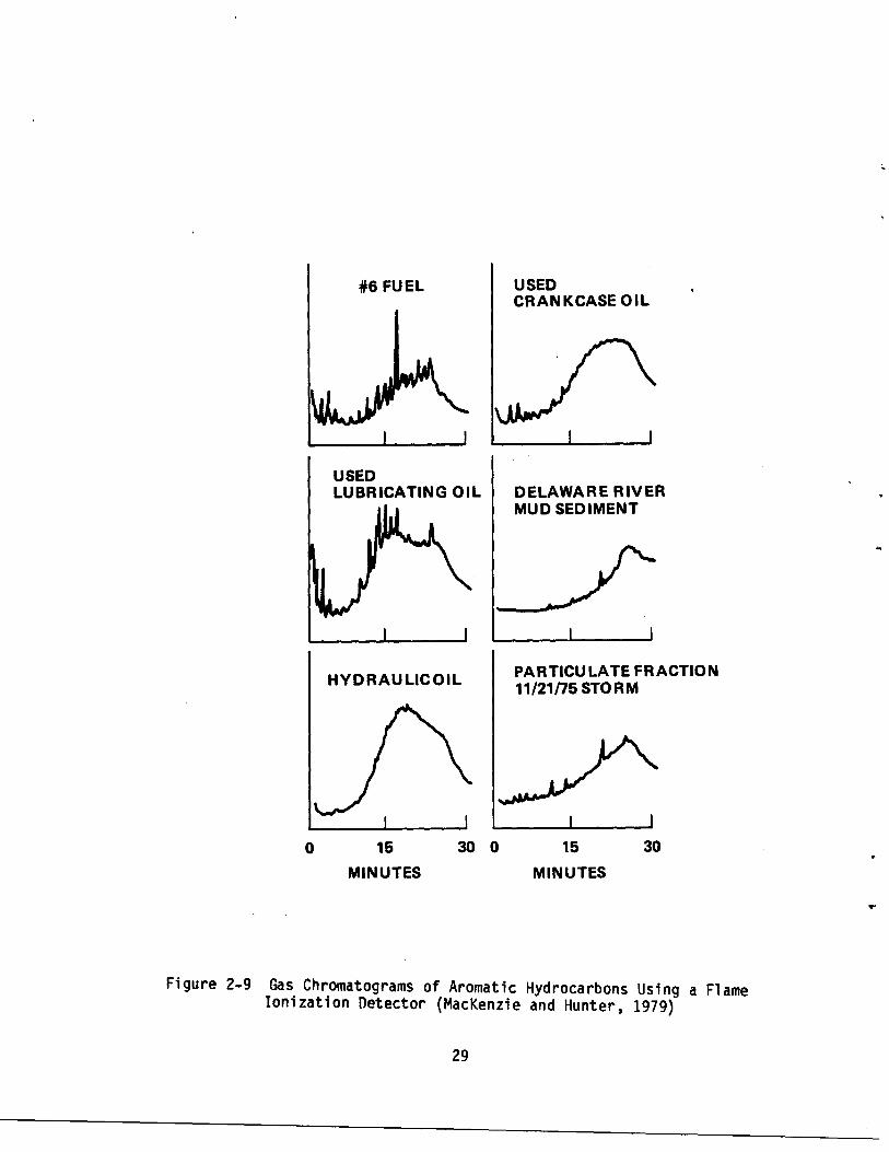
products to the gas chromatograms of the aromatic fractions of the particle

associated hydrocarbons from stormwater runoff. The particulate phase was

chosen for fingerprint analysis because it contained about 95 percent of the

total aromatics . Figure 2-9 shows the gas chromatograms of the aromatic

hydrocarbons associated with the stormwater particulates in the Delaware River

sediments and in some refined petroleum products using a flame ionization

detector (FID) . Figure 2-10 shows the simultaneous response with a sulfur-

specific flame photometric detector (FPD) system .

The source of the aromatic hydrocarbons in the stormwater sample is not .

obvious based on the FID fingerprint (Figure 2-9) . The FPD fingerprints,

however, are distinct, and the similarity between the stormwater and crankcase

oil fingerprints can be seen . On the basis of this information, Hunter and

MacKenzie concluded that while the high boiling, high molecular weight compo-

nents of several petroleum products may have contributed to the oil pollution

i n urban runoff, used crankcase oil appeared to be the most likely contribu-

tor .

All samples contained dibenzothiophene and phenanthrene and/or anthra-

cene . The average concentration of dibenzothiophene in the three storms

sampled ranged from 44 .2 to 62.3 ng/1 . Phenanthrene and anthracene could not

be differentiated on the column used (MacKenzie and Hunter, 1979) . The large

unresolved envelopes are thought to be composed primarily of four and five-

ring thiophenes as well as aromatic sulfides, thiols, and thianidans according

to Martin and Grant (1965) .

Another study which examined oil-and-grease-type compounds in urban

runoff was performed by Wakeham (1978) . The purpose of this study was to

determine the contributions of petroleum hydrocarbons from several suspected

sources to Lake Washington . Among the suspected sources investigated were

28

0

USEDLUBRICATING OIL

I I

DELAWARE RIVERMUD SEDIMENT

I I

II II

15

30 0

15

30MINUTES

MINUTES

PARTICU LATE FRACTION11 /21/75 STO R M

Figure 2-9 Gas Chromatograms of Aromatic Hydrocarbons Using a FlameIonization Detector (MacKenzie and Hunter, 1979)

29

#6 FUEL

USEDLUBRICATING OIL

III

HYDRAULICOIL I

30

II

IIII15

0 30

15MINUTES

MINUTES

USED

ICRANKCASEOIL

iDELAWARE RIVERMUD SEDIMENT

PARTICULATE FRACTION11 /21/75 STO R M

0

Figure 2-10 Gas Chromatograms of Aromatic Hydrocarbon Fractions Using a FlamePhotometric Detector-Sulfur Mode (MacKenzie and Hunter, 1979)

30

urban stormwater runoff from Seattle (3 sampling sites) and the runoff from

two freeway bridges which cross Lake Washington . Fifty stormwater samples

were collected over a 15-month period .

The bridge and urban stormwater runoff was collected in stainless steel

buckets and transferred to glass bottles prior to returning to the lab for

extraction and analysis . No attempt was made to collect samples at beginnings

of storms . Samples were extracted three times with pentane, and the pentane

extractables were subsequently charged to columns of alumina packed over

silica gel . The columns were then eluted with pentane. Following evaporation

of the pentane solvent, the elutes were weighed on an electrobalance . The

molecular composition of the aliphatic hydrocarbons was then analyzed by gas

chromatography using flame ionization detectors .

Wakeham (1978) observed that the chromatograms of urban and bridge runoff

water show primarily a large unresolved complex mixture of cyclic and branched

saturated hydrocarbons . In addition, he notes that odd-carbon chain length

paraffins are present in nearly equal concentrations as are paraffins with

even-carbon chain lengths. The presence of these two features are generally

indicative of petroleum-type hydrocarbons (Wakeham, 1978) . Wakeham also cites

the radio-carbon age (35,000 yrs) of the hydrocarbons as further evidence of

their petroleum origin .

Wakeham (1978) suggests that the petroleum hydrocarbons are due to dis-

charges of lubricating oils from automobiles . The evidence which he cites as

suggesting this source is the gas chromatogram pattern of a large unresolved

envelope coupled with small paraffin peaks (indicative of dewaxed lubrication

oils) . He notes the similarity of the chromatograms of used motor oil and

stormwater runoff, as shown in Figure 2-11 .

31

Transport Mechanisms

Between the time of the initial release of hydrocarbon pollutants at

their source and their final deposition by stormwater runoff into receiving

waters, chemical and physical processes take place that change the character

of the pollutant . One obvious change that occurs is the rapid evaporation of

lighter hydrocarbon fractions, making weathered hydrocarbon samples sharply

depleted in the low carbon range as compared to unweathered samples . Some

degradation of the hydrocarbon may occur at the original release site, but

this is essentially a slow process and depends strongly on the environment of

release . Hydrocarbons absorbed by soils may be completely degraded by

bacteria and never reach receiving waters . Hydrocarbons deposited on roadways

will undergo little or no degradation before transport to receiving waters .

The physical state of the hydrocarbons in stormwater is important because

it determines the fate of the pollutant in the environment and thus determines

its potential environmental effects . The design of mitigation measures is

also determined by the state of the hydrocarbons at the time of treatment .

Hydrocarbons in storm water can exist as free oil on the surface of the water

or adsorbed onto particles ; or as dissolved or colloidal oil mixed with the

water itself . Free oil can be skimmed from the surface, and particulates

settle out to be deposited in bottom sediments . Dissolved or colloidal oil is

difficult to remove, requiring some form of chemical intervention to separate

it out. Dissolved and colloidal hydrocarbons are also most hazardous environ-

mentally since they are most easily available for uptake by marine organisms .

As has been previously stated, about 85% of all hydrocarbons in urban

stormwater runoff are in association with particulates . These particulates

are separated from solution by filtering or by some gravimetric process such

as centrifugation .

They therefore include either agglomerations of oil

33

droplets, or solid particles with hydrocarbons adsorbed to their surfaces, or

most probably some mixture of the two . These two types of particulates are

indistinguishable with respect to their physical behavior although they are

chemically different .

It is not clear how the hydrocarbons come to be in conjunction with

particulates . Several mechanisms are possible . The hydrocarbons may drip

onto a surface and associate there with pre-existing particulates . They may

be originally emitted in conjunction with particulates as in emissions •from

automobile tailpipes or from stationary furnaces burning hydrocarbon fuel .

Agglomerations of hydrocarbons may form on dry surfaces and be picked up by

stormwater, or the agglomerations may form within the runoff stream .

Similarly, free or dissolved hydrocarbons can adsorb onto particle surfaces

during transport by storm water . Probably several, if not all, of these

mechanisms operate on the hydrocarbons found in urban storm water runoff .

Whatever the mechanism of association, it is clear that most hydrocarbons

in urban runoff are associated with particulates and therefore an understand-

ing of the transport dynamics of particulates is vital to an explanation of

the transport of hydrocarbons . A Washington D .C . study (Shaheen, 1975)

determined that the street dust and dirt fraction (particles less than 3 .35 mm

in diameter) is composed primarily of local minerals and materials abraded

from the road surface . 95% of this material is insoluble and inorganic .

Traffic dependent rates of deposition onto roads of total dust and dirt (2 .38

x 10-3 lb/axle-mile) were determined by this same study . While these

deposition rates are constant, the actual accumulation of pollutants on

roadways does not proceed at a constant rate but levels off after a time, as

shown in Figure 2-12 . Shaheen (1975) determined the ratio of pollutant

loadafter three days deposition to pollutant load after one day . The ratio

34

WJ

aaaz

Q G200

0JH

W3

0I

0Z 100Q

GJQF-0H

0 1 2

k2 = 1 x 10⁻⁵, Lm = 238 lbs/MILE

k2 = 3 x 10⁻⁵, Lm = 79.3 Ibs/MI LE

IIIIIIIIIII3 4 5 6 7 8 9 10 11ACCUMULATION PERIOD (DAYS)

IIIIIIIIIII0

4

8

12

16

20

24

28

32

36

40

44TRAFFIC (AXLESx 10+4)

(k1 -2.38x 10⁻³ lbs/AXLE-MILE, ADT - 40,000 AXLES)

Figure 2-12 Total Dust and Dirt Dry Weight Accumulations (Shaheen, 1975)

35

for particulates was 1 .43, and that for oil and grease was 1 .42 . The close

similarity of these ratios supports the evidence that hydrocarbons are

primarily associated with particulates . This leveling off of pollutant load

on roadways takes place in the absence of street sweeping or flushing by

storms . It is caused by removal of particulates from the road by winds and by

traffic action . Thus it appears that road surfaces have a saturation level

for particulates, and hence for hydrocarbons, since hydrocarbons are found

primarily in conjunction with particulates .

Sartor et al (1974) obtain similar results as shown in Figure 2-13, but

they interpret their data as showing a loading rate which decreases with time

to a small constant non-zero value . Thus the pollutant load would continue to

increase slowly, and surfaces would not saturate . There is insufficient data

at this time to decide between these two interpretations of the data .

The experimentally observed leveling off of pollutant load has various

effects on general storm water pollution . If the material blown off the road

is transported to another surface with a high runoff coefficient K, such as a

sidewalk or a parking lot, no net reduction in runoff pollution occurs .

However, if the particles end up on a low K surface such as a green belt, the

particles may be retained through storm events, yielding a net decrease in

pollution.

The tendency for particulate loading and thus for hydrocarbon loading to

level off with time makes it less likely that the time between storms will be

proportional to hydrocarbon pollutant levels . It is possible that the partic-

ulates on roadways will become more saturated with hydrocarbons as the time

between cleaning or storm events increases . This seems consistent with the

theory that total storm pollutant load is independent of the time since the

previous storm, but that the degree of concentration of hydrocarbons in

36

1400W

•1200

ccny

1000C7ZG4 8000JN0J 600

0

I I I I I I I

I

I( •) INDUSTRIAL

"ALL" LAND - USECATEGORIES COMBINED

0 1 2

3

4

5

6

7

8

9

10

11

ELAPSED TIME SINCE LAST CLEANING BY SWEEPING OR RAIN (DAYS)

Figure 2-13 Accumulation of Pollutants by Land Use (Sartor et al, 1974)

37

12

the first flush is a function of the length of the antecedent dry period

(Weibel, 1964) . Highly saturated surface particulates from roadways would

probably be strongly represented in the first flush waters .

The dynamics of particulate transport would allow extraneous factors to

influence particulate concentration and hence hydrocarbon concentration in

storm waters . Consider two identical storms preceded by the same number of

dry days . If one storm is preceded by high winds that blow hydrocarbon

bearing particulates out of the area, or off of high K surfaces, such as

roads, and onto low K surfaces such as open land, the runoff waters from that

storm will have lower hydrocarbon concentrations . Hydrocarbon concentration

can easily be influenced by winds since the smallest particulate fraction,

which are most vulnerable to wind transport, contain the greatest proportion

of hydrocarbons .

Oil and grease accumulation rates for various land uses were estimated

for the EPA's Storm Water Management Model (SWMM) (Huber et al, 1975 ; Metcalf

and Eddy Inc ., 1971) . These rates, which are based on engineering judgement

and not on experimental data, are presented in Table 2-5 . Shaheen (1975)

reports that land use does indeed affect accumulation rates . The SWMM esti-

mated rates are constant and do not include the leveling off with time which

is experimentally measured by Shaheen (1975) and Sartor et al (1974) . For

this reason accumulation is taken to be proportional to the time since the

previous storm .

Road characteristics also have an effect on pollutant loads . Shaheen

(1975) reports that high curbs allow larger concentrations of particulates by

acting as wind shields . Figure 2-14 shows his results . Where curbs are lower

the particulate distribution contains fewer smaller particles which are more

38

39

TABLE 2-5 GREASE ACCUMULATION

Type

(Metcalf and Eddy Inc ., 1971)

Land Use mg/dry day/100 ft-curb

1 Single family residential 318

2 Multiple family residential 1,044

3 Commercial 1,498

4 Industrial 2,088

5 Undeveloped or park 681

5

4

3

2

O

IIII0

10

20

30

40ROADWAY BARRIER HEIGHT (INCHES)

Figure 2-14 Per Axle Dry Weight Loading vs . Roadway Barrier Height(Shaheen, 1975)

40

o LITTER - LOW SPEED LANES

LITTER - HIGH SPEED LANES

0 DUST& DIRT- LOW SPEED LANES

DUST& DIRT- HIGH SPEED LANES

DUST& DIRT

O

O

LITTER

I

easily transported over the barrier by winds . For any curb height, the great-

est concentration of pollutants is found near the curb (Sartor et al .,

1974) . Shaheen (1975) proposes two alternate ways in which this effect may be

utilized . Roadways could be built without curbs to allow wind transport of

particulates to adjoining greenbelts . Conversely, high curbs could be built

to trap particulates, especially the smaller size fractions that carry the

most hydrocarbons . These roadways would then be mechanically cleaned periodi-

cally. A difficulty with this concept is that if cleaning were not frequent

enough, the roadways with their high curbs would provide a very efficient

system for transportation of hydrocarbons to receiving waters during storms .

Also it is known (Shaheen, 1975 ; Sartor et al, 1974) that street sweeping

efficiency falls off greatly for smaller particulates . Thus the particles

most likely to be left behind by traditional mechanical cleaning methods are

precisely those it is most important to remove .

Road surfacing material also influences the degree of particulate pollu-

tion (Russell and Blois, 1980 ; Sartor et al, 1974), with concrete surfaces

contributing fewer particulates and hence less hydrocarbons than does

asphalt . Road surface condition is cited as an important criterion in some

studies (Sartor et al, 1974), and is considered unimportant in others (Russell

and Blois, 1980) . Poor road surfaces can provide local areas for high produc-

tion and retention of particulates, producing high hydrocarbon content in

storm runoff.

Summary

Hydrocarbons in urban stormwater runoff are found mostly in association

with particulates . Since particulates are a major pollutant in stormwater

runoff (Sartor et al, 1974 ; Sonderlund and Lehtinen, 1972), perhaps

41

Is

hydrocarbon removal can best be accomplished in conjunction with particulate

removal . More work is required to identify the percentage contributions of

the various hydrocarbon sources to pollution . Crankcase oil has been identi-

fied as a major contribution, and the consistently higher contributions from

roadways than from residential sites implies that emissions during vehicle

operation either from engine leakage or crankcase drippings are a more

important source than illegal dumping . Since the GC profile of tailpipe

exhaust so closely resembles that of crankcase oil, further study is required

to differentiate between these sources to better determine source control

measures .

42

CHAPTER 3

BIOLOGICAL EFFECTS OF OIL AND GREASE

Introduction

In the past decade, interest in the biological effects of hydrocarbons on

marine organisms has increased as efforts have been made to control signifi-

cant pollutant releases into the marine environment . A large body of litera-

ture on the effects of hydrocarbon pollution on marine organisms has been

published and several recent review articles (NAS, 1975 ; Anderson, 1979 ; AIBS,

1976 ; Malins et al, 1977 ; API, 1977) have summarized the results of recent

studies and assessed the current state of knowledge on the effects of oil

pollution .

Most of the work done on the biological effects of oil on marine life has

been in response to oil spills . However, petroleum-derived hydrocarbons are

regularly released into estuarine environments in proportion to surrounding

urbanization and technological developments (Di Salvo et al, 1975) . Both the

quantity and the quality of oil from spills may differ significantly from that

in urban runoff, resulting in substantially different effects on the marine

environment . Spills expose marine life to much higher concentrations at any

one time than oil and grease from surface runoff .

Oil Types

The types of petroleum or petroleum products most commonly released into

the marine environment are crude oils, Bunker C or No . 6 fuel oils, diesel or

No. 2 fuel oils, and light petroleum products such as kerosenes or gasolines

(NAS, 1975) . The composition of these oils are significantly different .

Bunker C fuel oils are the heaviest distillate fractions of petroleum . The

43

great majority of compounds in Bunker C oil in the C30+ range, and typically

consist of 15% paraffins, 45% naphthenes, 25% aromatics, and 15% polar NSO

compounds .

No . 2 fuel oils represent a middle distillate fraction of petroleum

composed almost entirely of hydrocarbons in the range C12 to C 25 . By molecu-

lar type, 30% are paraffins, 45% are naphthenes, and 25% are aromatics .

Light petroleum products are made up of virgin and cracked components .

Kerosene contains hydrocarbons in the C10 to C12 molecular weight range,

typically 35% paraffins, 50% naphthenes, and 15% aromatics . Gasoline contains

hydrocarbons in the range C5 to C 10, typically 50% paraffins, 40% naphthenes,

and 10% aromatics for virgin gasoline and 20 to 30% aromatics in blended

gasoline (NAS, 1975) .

Oil in Urban Runoff

The predominant contributor to oil and grease in urban runoff is most

likely used automotive crankcase oil, a refined distillate petroleum product .

Wakeham (1977) attempted to characterize the sources of petroleum hydrocarbons

in Lake Washington and collected data suggesting that hydrocarbons from urban

stormwater runoff come from discharges of lubricating oils from automobiles .

Whipple and Hunter (1979) concluded that petroleum hydrocarbons in urban

runoff resemble used crankcase oil and contain toxic chemicals such as the

polynuclear hydrocarbons, naphthene, pyrene, fluoranthene, chrysene, and benzo

(a)-pyrene .

Once released into the environment, crankcase oils may undergo consider-

able modifications before they enter the marine environment . Oils exposed to

the atmosphere may become extensively "weathered" which primarily involves the

evaporative loss of lower molecular weight hydrocarbons from the oil- water

44

mixture, leaving behind the heavier molecular weight component (Garza and

Muth, 1974 ; MacKenzie and Hunter, 1979) .

Crankcase oils have different components than crude oils and fuel oils .

Crude oils and fuel oils contain homologous series of n-alkanes and branched

alkanes, napthenes, aromatic hydrocarbons, and non-hydrocarbon components,

(Farrington and Quinn, 1973) . Lubricating oils, however, are usually dewaxed,

that is the n-alkanes and branched alkanes are removed (Farrington and Ouinn,

1973 ; Blumer et al, 1970) .

Oil Toxicity

The soluble fractions of petroleum are probably the most harmful to

marine organisms . Discharges into estuaries may be especially damaging since

they pollute shallow water areas that serve as nursery areas for many coastal

marine biota (NAS, 1975) . Toxicity may vary widely among different types of

oil because the composition and concentration of individual hydrocarbons

present in the oil varies . Anderson et al (1974) found that the water soluble

fractions of crude oils were richer in light aliphatics and single-ring

aromatics than the water soluble fractions of refined oils, which contained

higher concentrations of naphthalenes . In general, the water solubility of

hydrocarbons drops drastically as one goes to higher carbon numbers . Solu-

bility can also change with degradative processes ; for example, naphthalene

(solubility, 32 pm) can be oxidized to d-naphthol (solubility, 740 ppm) (NAS,

1975) . Rich et al (1977) have made a number of observations on the compar-

ative toxicity of oils :

1 . Toxicity of crude and refined oils depends on the concentration of toxic

compounds in the oil and on physical factors, such as the temperature and

45

viscosity of the oil, which affect transport of petroleum hydrocarbons

into the water .

2 . Refined oils are generally considered more toxic than crude oils because

they often have higher concentrations of aromatic hydrocarbons and are

usually less viscous than crude oils .

3. Oil toxicity is apparently due to the soluble compounds in the water

rather than dispersed droplets .

4. Toxicity of aromatic hydrocarbons increases with the number of rings and

with the degree of alkyl substitution . Solubility decreases with these

factors so that the relative importance of individual aromatic hydro-

carbons to toxicity of water soluble fractions is unknown . Mono- and

dinuclear aromatics probably account for most of the toxicity in water

soluble fractions .

Recent results suggest that aromatics, in particular naphthalene and

naphthalene type compounds, are probably the most toxic (De Vries, 1979) .

Table 3-1 summarizes the data from several studies on the comparative

toxicity of different aromatic hydrocarbons . The results are quite consistent

for the six species tested . Mono-aromatics are the least toxic ; acute

toxicity increases with increasing molecular size up to the four-and five-ring

aromatic compounds which have very low water solubility . Increasing the

number of side chains on the aromatic nuclears (alkylation) of one, two, and

three-ring compounds, such as benzenes and naphthalenes, results in higher

toxicity . The position of side chains may also influence the toxicity of

aromatics (Caldwell et al 1977) .

To a certain degree, it is possible to predict the toxicity of a given

oil based on the relative concentration of toxic aromatics present in the

oil . For example, No . 2 fuel oil is more toxic than crude oils since it

46

1Neff et al (1976) . Neanthes araenaceodentata

2Neff et al (1976) . Palaemonetes pugio

Caldwell et al (This symposium) . Cancer magister, Stage I larvae

4Benville and Korn (In press) . Coo fraciscorum

5Benville and Korn (In press) . Morone saxatilis

6Brenniman et al (1975) . Carassius auratus

3

47

TABLE 3-1

COMPARATIVE TOXICITY OF DIFFERENT AROMATIC HYDROCARBONS,EXPRESSED IN 96-HR LC ~~ 'S WITH CONCENTRATIONS IN PPM . ASTERISK(*) INDICATES THAT TOXIC CONCENTRATIONS WERE ABOVE SOLUBILITYLIMITS (Rice et al, 1976) .

AROMATIC H.C .96-hr LC50 's in ppm

POLYCHAETE 1 SHRIMP2 CRAB LARVAE3 SHRIMP4 BASS5 GOLDFISH

Benzene -- 27 108 20 5 .8-10.9 --

Toluene -- 95 28 4.3 7 .3 22.8

Ethyl benzene -- -- 13 0 .5 4 .3 --

Tri-methyl benzene -- 5.4 5 .1 -- -- 12.5

Xylene -- 7 .4 -- -- -- 16.9

m- -- -- 12 3 .7 9.2 --

o- -- -- 6 1 .3 11 .0 --

p- -- -- -- 2 .0 2 .0 --

Naphthalene 3 .8 2 .4 >2

Methyl naphthalene -- 1 .1 1 .6

Di-methyl naphthalene 2 .6 0.7 0.60

Tri-methyl naphthalene 2 -- --

Phenanthrene 0.6 -- --

Methyl phenanthrene 0.3 -- --

Fluorene 1 -- --

Fluoranthrene 0.5 -- --

Chrysene * -- --

Benzo-(a)-pyrene * --

1,2,5,6-Dibenzanth racene * -- --

contains more aromatics (NAS, 1975) . Crankcase oils have been shown to be

particularly toxic to aquatic organisms . Virgin crankcase oils contains

relatively high concentrations of polycyclic aromatics (PAH) as a result of

considerable refining and processing (Neff, 1976) .

PAH (naphthalenes and phenanthrenes) have high toxicity and persistence

in the marine environment (Linden et al, 1979) . The presence and concentra-

tion of specific PAH in oil are influenced by a number of factors including

the composition of the crude oil from which the petroleum product is derived,

and refining conditions such as temperature and catalysts . Carcinogenicity

observed in human or in experimental animals following exposure to some

materials derived from fossil fuels appear to be partly due to polycyclic

aromatic hydrocarbons (Bingham and Yolk, 1969) .

Payne et al (1978) have tested the mutagenicity of crude oils and both

new and used crankcase oil fractions toward Salmonella typhimurium strain TA-

98 . Positive results were obtained only with used crankcase oils ; however, it

appears that compounds other than benzopyrene or benzanthracene (which are

produced in automobile engines) are the major mutagenic sources . Previous

work had demonstrated that fish taken from sites with a history of oil contam-

ination had elevated AHH (aromatic hydrocarbon hydroxylases) levels . AHH are

enzymes involved in the bioactivation of aromatic compounds to mutagens in

mammalian systems and are known to occur in most marine organisms . In some

mammalian systems there is a relationship between AHH activity and susceptibi-

lity to hydrocarbon-induced cancers . This may have implications for human

health since hazards to humans could come from eating oil-contaminated sea-

food, particularly if carcinogens such as polycyclic aromatic hydrocarbons

(PAH) are present (NAS, 1975) .

48

Petroleum hydrocarbons that combine with other organic and inorganic

substances in water and sediments such as pesticides, PCBs, and chlorine

compounds may be considerably more toxic than each substance by itself (Blumer

et al, 1977 ; Laughlin et al, 1978) . The synergistic effects of these combined

products may also result in greater fat solubility and high bioaccumulation

potential . The photooxidation of oils may produce toxic hydrocarbon products

or increase the toxicity of oil constituents (Payne et al, 1978) .

PetroleumHydrocarbonsinWaterandSediments

The fate of petroleum hydrocarbons released into the marine environmental

is not completely understood . However, transient storage compartments include

water, marine organisms, and sediments, with sediments probably being the most

significant long-term storage site (Di Salvo et al , 1975) . Losses of hydro-

carbons from the system may occur through evaporation, tidal and riverine

flushing, and microbial degradation . Farrington and Quinn (1973) have

provided some evidence for these processes in the marine environment with

their analysis of hydrocarbons in surface sediments and clams (Mercenaria

mercenaria) in Narrangansett Bay.

In another study, clam (Tapes japonica, Mya arenaria) and mussel (Mtyilus

edulis) samples from around the Bay Area were found to be contaminated with

different concentrations of hydrocarbons (Guard, 1981) . Hydrocarbon tissue

contents, analyzed by thin layer chromatography, ranged between 20 ppm to

220 ppm, from the cleanest to dirtiest point . Interestingly, the majority of

the unsaturated fraction of hydrocarbons seemed to be composed of highly

alkylated mono- and di-aromatics . Previous work by MacKenzie and Hunter

(1979) reported a disappearance of diaromatics through weathering in urban

runoff . This could suggest that the hydrocarbons found in clams and mussels

49

analyzed might come from oil directly spilled into the bay rather than from

automotive lubricative oil in stormwaters .

Other studies have also shown that petroleum hydrocarbons can accumulate

in bottom sediments . Often, these accumulated hydrocarbons undergo little

breakdown and are released into the water column over an extended period of

time. Thus, polluted sediments are a major source of chronic hydrocarbon

pollution .

Blumer (1970) found that essentially unaltered No . 2 fuel oil was present

in sediments two months after a major spill and that various components of the

oil were being released into the water. MacKenzie and Hunter (1979) and

Wakeham (1977) found that river and lake bottom sediment accumulated petroleum

hydrocarbons from storm-water runoff and that little degradation of the most

toxic oil fractions had occurred . The major contributing pollutant in these

studies was found to be used crankcase oils . Petroleum hydrocarbons tend to

accumulate in sediments for the following reasons :

1 . Hydrocarbons adsorbed to particulate matter settle out of the water column

as they become heavier and less soluble .

2 . Petroleum hydrocarbon degrading bacteria preferentially attack low molecu-

lar weight, straight chain hydrocarbons, leaving other oil constituents

behind, and

3. As oil components are degraded, oxygen is depleted in the sediments, .

preventing further breakdown (Farrington and Quinn, 1973) ; MacKenzie and

Hunter, 1979) .

Oil pollutants in sediments can concentrate' fat-soluble poisons by acting

as "partitioners" to retain substances which have a low solubility in water

but a higher solubility in petroleum hydrocarbon mixtures . Oil pollutants may

adsorb to particulate matter containing toxic organic compounds such as DDT or

50

PCBs and chemically interact with these and other adsorbed constitutents

(Blumer et al, 1970 ; Mackenzie and Hunter, 1979) . Hydrocarbons may also

combine with chlorine compounds to produce chlorinated hydrocarbons (Whipple

and Hunter, 1979) . Hartung and Linger (1970) found that combined levels of

chlorinated hydrocarbons in river sediments approached levels similar to

insecticide applications and that such polluted areas were devoid or very

deficient in benthic arthropods . Numerous investigations have shown that

bacteria preferentially metabolize n-alkanes and branched alkanes relative to

naphthenic and aromatic hydrocarbons (Farrington and Quinn, 1973) . Bacterial

degradation has little effect on the less soluble aromatics and higher molecu-

lar weight compounds (Tanacredi, 1977) . Since hydrocarbon in urban runoff

appears to consist primarily of used crankcase oils which contain relatively

high concentrations of higher molecular weight compounds especially if

weathered, bacterial decomposition is not likely to be extensive. Wakeham

(1977) found that hydrocarbons entering Lake Washington from urban runoff are

not rapidly dispersed or degraded by microorganisms but they are being incor-

porated in increasing concentrations in lake sediments .

EffectsonMarineOrganisms

The toxic effects of oil pollution may be acute or sublethal . Although

sublethal effects do not kill an organism outright, they may reduce the

ability of marine organisms to survive and reproduce in their normal environ-

ment (Linden et al, 1979), effectively eliminating some species over a longer

period of time .

The standard method for determining lethal concentrations of petroleum

hydrocarbons is to expose aquatic species to various concentrations of the

test substance for a given time period, usually for 96 hours . The minimum

51

concentration that produces mortality in half of the population at the end of

the exposure period is considered lethal . This concentration is designated as

the 96-hour LC5 0 or TLm . Neff et al (1976) reported a 96-hour LC50 of 0.3 to

0 .6 ppm for the aromatic compounds, 1-methylphenanthrene, fluoranthene, and

phenanthrene in the polychaete, Neanthes arenaceodentata . The toxicity (96-

hour LC50) of crude oil in water to a variety of adult marine fish and inver-

tebrates tested in static exposures ranges from one to 20 ppm. For No . 2 fuel

oil, the range is 0.4 to 6 ppm (Anderson, 1979) .

Hyland and Schneider (1976) as noted in Laughlin et al (1978) concluded

that lethal effects of soluble aromatic hydrocarbon fractions occur in the one

to 100 ppm range for adults and in the range 0 .1 to 1 ppm for larvae and

Juvenile forms . Investigations have also indicated that very high concentra-

tions associated with sediments are required to produce ~mortality . Lack of

significant mortality is observed during exposure to concentrations in excess

of 1,000 ppm (Anderson, 1979) .

The wide variation of measurements and methods used in chemical toxicity

studies makes it difficult to extrapolate the results from one study to

another or from laboratory populations to natural populations . When assessing

the potential impact of exposure to oil, it is crucial to know if some species

or life stages are more sensitive than others to oil toxicity (Rice et al,

1977) . It should be noted that historically most toxicity studies have been

conducted with organisms capable of adapting to laboratory conditions, not the

most sensitive species (Tatem, 1977) .

Of greater concern in the case of urban runoff are the effects of suble-

thal concentrations of petroleum hydrocarbons on marine organisms . Sublethal

concentrations are generally considered to be two orders of magnitude less

than lethal concentrations for a given species, with lower concentrations

52

considered "safe" (Anderson, 1977) . Sublethal effects could result in reduc-

tion of populations in the field (Tatem, 1977) . Linden (1976) and Wells and

Sprague (1976) have found larval development and growth to be affected by low

levels of petroleum hydrocarbons . Wells and Sprague have stated that the

ratio of "safe" to acutely lethal concentrations of petroleum hydrocarbons was

0 .03. This means that for many estuarine organisms which have acute LD50

values of 1 .0 to 2 .0 ppm, water concentrations remaining above 30-50 ppb for

any length of time could be harmful (Tatem, 1977) .

It is difficult to determine what parameters represent a reliable and

sensitive method for determining the condition of an organism or the extent of

stress on the animal following exposure to hydrocarbons . Respiration, osmotic

and ionic regulation, behavior effects, growth and reproduction, morphological

and histological effects, and biochemical alternations have all been suggested

as indicators . Respiration has been used most frequently to determine the

extent of stress (Anderson, 1977) . Measurements of respiratory rate during or

after exposure to No . 2 fuel oil indicate that a range of 0.1 to 0 .85 ppm

total naphthalenes produces a response that differs significantly from those

of control animals . Tissue analyses show measurable amounts of naphthalene

during this time (Anderson, 1977) .

Anderson (1977) has summarized some recent studies used to determine the

effects of petroleum hydrocarbons on growth and reproduction . These results

are shown in Table 3-2 . The concentrations of both total hydrocarbons and

total aromatics shown to reduce growth and/or survival range from about 0.2 to

10 ppm .

There are few adequate studies on behavioral effects . The fish, Fundulus

similus exhibits abnormal behavior at brain concentrations of 200 ppm.

Suppression in the locomotor activity of an amphipod and a coelenterate medusa

53

TABLE 3-2 SUMMARY OF EFFECTS OF PETROLEUM HYDROCARBONS ON THE GROWTH AND REPRODUCTION OF MARINE ANIMALS

Exposure Concentration (ppm) 1 Growth or ReproductionSpeciesOil(days)THTNTAParameterReference

FISHFundulus similus

Cyprinodonvariegatus

Oncorhynchusgorbuscha

DECAPODSCancer magister

Rithropanopeusharrasii

Palaemonetespugio

ParaIithodescamtschatica

Pandalushypsinotus

Homarusamericanus

So .La .C2

20

16.0

0.2

9.7

4% hatch of eggs

Anderson et al, 1979

No .2 F03

7

2.0

0.6

1 .7

0% hatch of eggs

Anderson et al, 1979

Prudhoe

10

0.7

Reduced growth rate

Rice et al, 1975Crude

of pink salmon fry

Alaskan

60

0.2

Reduced survival of

Caldwell et al, 1977Crude

zocae on long-termexposure

No . 2 FO

27

1 .0

0.3

0.9

Reduced survival and

Neff et al, 1976extended developmentto megalopa

No . 2F0

27

0.9

0.3

0.8 Reduced growth rate

Tatem, 1977larvae

3

1 .4

0.6

Reduced viability ofeggs from exposedgravid females

Cook Inlet 1-4Crude

Cook Inlet 1-4Crude

Venezuelan

30Crude

1 .6

Inhibition of molting

Mecklenburg,in larvae

1 .2

Inhibition of moltingin larvae

(continued)

1977

0 .14

30 day LD5(t and re-

Wells and Sprague, 1976tarded development oflarvae

TABLE 3-2 (continued)

Growth or ReproductionParameter

Reference

Reduced growth rate

Linden, 1979of larvae

Reduced growth rate

Rossi, 1976of larvaeReduced growth of

Anderson, 1979juveniles by 30%

Reduced survival and

Carr and Reish, 1977reproduction

1TH, total hydrocarbons ; TN, total naphthalenes : TA, total aromatics

2 South Louisiana Crude Oil, API reference oil

3High aromatic (38%) No .2 Fuel Oil, API reference oil

11

4

Species OilExposure(days)

Concentration (ppm) 1TH

TN

TA

AMPHIPODSGammarus Crude 60 0 .3-0 .4

oceanicus

POLYCHAETESNeanthes No .2 FO 22 1 .0 0.3 0.9arenaceodentata

No .2 FO 28 0.3 0.1

Ctenodrilus No .2 FO 28 2 .2 0 .5 1 .4serratus

So .La .C 28 9.9 0.2 7 .0

Ophyrothrocha sp No .2 FO 28 1 .3 0.3 0 .9So .La .C 28 9.9 0 .2 7 .0

was observed after exposure to extracts of four oils at 15 ppm or greater

(Anderson, 1979) . In general, levels of 0 .1 to 0 .3 total naphthalenes,

regardless of the oil, appear to be the lowest concentrations in water which

produce abnormal and deleterious responses during long-term exposure to sub-

lethal levels of petroleum hydrocarbons .

Bioaccumulation is an additional concern with oil pollution . Bivalves

tend to slowly and constantly accumulate hydrocarbons while fish and shrimp

take up hydrocarbons very rapidly, reaching maximum levels within a few hours

(Anderson, 1979) . Accumulation of aromatic hydrocarbons in tissues of marine

animals appears to be dependent on partitioning of the hydrocarbon between the

exposure water and the tissue lipids (Neff et al, 1976) . When animals are

returned to oil-free seawater, they rapidly release accumulated hydrocarbons

from their tissues . Release usually takes 2 to 60 days, depending on the

species (Neff et al, 1976) .

Lee (1977) has reviewed studies on the accumulation and turnover of

petroleum hydrocarbons in marine organisms . Zooplankton can take up a variety

of aromatic and paraffinic hydrocarbons from either food or water . Most of

the aromatics are lost in depuration studies with a half life of 2 to 3

days . Crustaceans (shrimp, crab, lobsters) can also take up hydrocarbons from

food or water.

Depuration varies with species . Deposit-feeding worms take up organic

pollutants associated with sediments . Bivalves take up and concentrate hydro-

carbons from water . A small amount of hydrocarbons are retained for a longer

period after the initial, rapid depuration . Table 3-3 summarizes some results

of studies on the toxicity of petroleum hydrocarbons to marine animals . The

experiments present evidence that sublethal concentrations of petroleum

hydrocarbons may have an adverse effect on marine organisms . Most of the

56

Compound Tested

Species

Experiment

No. 2 fuel oil

Neanthes arenaceodentataSo. Louisiana crude,

Capitella ca itataBunker C .

(poly ha e

No. 2 fuel oil,

5 polychaetes :So. Louisiana crude

Ophryotrocha sp .0 puerilisttenodrilus serratusCa itella cap tataCirrriformia spirabrancha

Q

TABLE 3-3 TOXICITY OF SELECTED MARINE ORGANISMS EXPOSED TO PETROLEUM HYDROCARBONS

Laboratory-reared polychaetesexposed to WSF* of oils

Laboratory-reared polychaetesexposed to WSF of oils

2 .24 .1

>8.7

96-hr TLm (crude oil)12.9 ppm

(continued)

Observations

References

WSF of No.2 fuel oil more toxic

Rossi et al, 1976 ;than WSF of crude. For No . 2 oil

Rossi and Anderson,48-hr TL, - 3.2 ppm (Neanthes) 48-

1976hr TLm - 3.5 ppm (Capitella) . Adultsmore susceptible than juveniles .

96-hr TLm (No. 2 fuel oil)

Carr and Reish, 19772.9 ppm

>8.7

Both species have a mixed function

lee et al, 1979oxidase system that metabolizes PAH

Breathing rates of fry exposed to

Thomas and Rice, 1979toluene and naphthalene immediatelyincreased . 24-hr TLm , 12°C deter-mined :

411 4

17 .2>19.8>19.8>19.8

Suppression of reproduction atlower concentrations .

Crude oil Capitella capitata Laboratory studies with oilBenz (a) anthracene Nereis virens mixed into sediments

Toluene, naphthalene, Oncorhynchus gorbuscha Exposure to WSF at 4°C and 12°CCook Inlet crude, (pink salmon)No . 2 fuel oil

5 .38 ppm toluene0 .92 ppm naphthalene1 .73 ppm aromatic hydrocarbons

from crude WSF0.65 ppm aromatic HC from No . 2

fuel oil WSF

Crude oil(Prudhoe Bay)

No . 2 fuel oil

No. 2 fuel oil

PAH

TABLE 3-3 (continued)

Observations

References

Fish take up naphthalene at concen- De Vries, 1979trations as low as 0.025 pm. Tendsto concentrate in the liver . Fishexposed to 1 ppm refused to feed,exposure caused lower rate of 02consumption, morphological changesin liver cells .

Macoma inquinata

Laboratory and field studies,

Behavior indicated stress ; reduced

Roseijadi and Anderson

cam

exposure at 1,000 ug oil/9

survival ; decrease in free amino

1979sediment

acid levels in muscle and mantle ;deterioration in physiological stateas indicated by "condition index" .

Fundulus heteroclitus

Embryos and larvae exposed

Hatching success decreased as WSF

Sharp et al, 1979(estuarine killitish)

to WSF in laboratory

increased. Embryos exposed to 25%WSF take up naphthalenes in tissuesdepressed heart beat rate and 0 2 con-sumption. Nine day biomagnificationfor naphthalenes was approximately 137 .

Rhithropano eus harrissi

Crabs exposed continuously after(mud crabs)

after hatching to WSF containing0.36 ppm total naphthalenes,1 .26 ppm total hydrocarbonstotal hydrocarbons ; 0.1 to 0 .3 ppmtotal-naphthalenes .

Studies on uptake, metabolism anddischarge of naphthalene and 3,4 -benzopyrene

Gillichthys mirabilis(sand goby)Oli ~ocottus maculosus(sculpin)Citharichthys stigmaeus(sand dab)

(continued)

Acutely toxic to zoeal stages .

Laughlin et al, 1978Crabs able to recover from effect ofchronic exposure . Sublethal concen-trations to larvae were 0 .3 to 0.9 ppm

All 3 species took up more naphtha-

Lee et al, 1972lene than benzopyrene . Fish tooklonger to flush out naphthalene .Gall bladder was a major storagesite .

Compound Tested Species

Experiment

Naphthalenes Myoxocephalus (sculpin) Laboratory studies on physiologyand biochemistry upon exposure

0

(D) USED MOTOR OIL

22I

20

--COLUMNBLEED

IIIIIIIIIIIIIIIIIIIII10 20

MINUTES30

40

Figure 2-11 Gas Chromatograms on Apiezon L of Aliphatic Hydrocarbons(Wakeham, 1978)

32

Waste oil

Petroleum Hydrocarbons

Mercenaria mercenaria(clam)

No. 2 fuel oil

t

(oyster)Penaeus aztecus (shrimp)

Mytilus edulisM tl us call-oni anusI

s)

Palaemonetes u io(grass shrimp

Field studies

TABLE 3-3 (Continued)

Analysis of hydrocarbons insurface sediments and clams fromNarrangansett Bay

Exposure to 2.6 ppm petroleumhydrocarbons and 0 .55 ppm totalnaphthalenes

(continued)

It

Observation

References

Clams exposed for 24 hr to 6 .28 ppm Neff et al, 1976total dissolved hydrocarbons accumu-lated 13.6 ppm total naphthalenes intissues . Clams accumulated BaP intissue at 236-fold concentration-BaPslowly released over 30-58 days .Naphthalenes were the aromaticaccumulated to the highest concen-tration by oysters . Shrimp and fishaccumulate aromatics rapidly -tissue concentrations often reachmaximum level within first hour ofexposure. All species releasedhydrocarbons after exposure .

Mussels transferred from clean

Oi Salvo et al, 1975water stations to polluted stationstook up hydrocarbons . When replacedin clean water, hydrocarbon contentapproached clean water baselinevalues .

Sediments and clams contaminated by Farrington and Quinn,petroleum hydrocarbons .

1973

After six hours, tissue levels of

Tatem, 1977methylnaphthalenes were 150 timesgreater than water levels ; sublethaleffects occurred at concentrationsof less than 0.5 to 1 .0 ppm .

4

Compound Tested Species Experiment

No. 2 fuel oil Ran is cuneata (clam) Laboratory exposureCrassostreaavirginica

No . 2 fuel oil

Fundulus heteroclitus

Combined effects of salinity,(estuarine killifish) temperature, and chronic exposure

of WSF on survival and developmentof embryos .

Crude oils,

C prinodon variegatus

WSF toxicity determinedNo. 2 fuel oil

(heepshead minnow)Bunker C fuel oil

Menidia ber llinas verside)Fundulus similus (fish)enF aeusaztecus post larvae(brown s r mpPalaes pugio(grass

shrshrim p'

Mysidopsis almyra

Crude,

Gamnarus oceanicus

Acute and sublethal exposuresNo . 1 light fuel oilNo . 4 heavy fuel oil

* WSF = Water Soluble Fraction

Observations

Reference

For concentrations up to 450 ug/l,

Stegeman and Teal, 1973initial rate of uptake directlyrelated to concentration . Uptakeapproached equilibrium after 5-6weeks . After 4 weeks of depuration,concentration remained at levels over30 times higher than those prior toexposure

0 .47 ppm total naphthalenes highly

Linden et al, 1979toxic under all conditions . Exposureto oil decreases time interval betweenfertilization and hatching

4R-hr TL, at 8.7 ppm total hydro-

Anderson et al, 1974carbon levels from No . 2 fuel oil

Larvae several hundred times more

Linden, 1976sensitive than adults during acuteexposure. Sublethal effects onadults include impaired swimmingperformance, impaired light reaction,decreased tendency to precopulate,decreased larval production .

TABLE 3-3 (continued)

Compound'Tested Species Experiment

No . 2 fuel oil Crassostrea virginica Exposure to various concentrations(oyster)

-

as follows :C. variegatus 43 ppmA. beryllina 40 ppmF. similus 23 ppmF. aztecus 9.4 ppmF. pug_~o 3.4 ppmR.

a 1 .3 ppm

experiments were laboratory studies in which the selected species were exposed

to the water soluble fractions of No . 2 fuel oil or crude oil, which are not

the oil types expected to be present in urban runoff . The toxicity of these

oils depends on their water-soluble hydrocarbon concentration (Carr and Reish,

1977) . None of the studies on marine organisms tested crankcase oil toxicity

and it is not clear that the results of these studies can be extrapolated to

different oil types or to a non-laboratory situation . In one study on the

effects of various oils on freshwater benthic algal communities, No. 2 fuel

oil was the most damaging, used crankcase oil was least toxic and Nigerian

crude oil was intermediate in degree of effect on metabolism (Bott et al,

1978) .

EcologicalEffects

Petroleum hydrocarbons, either in the form of a highly concentrated

release as in an oil spill or from chronic inputs can have far reaching

effects on aquatic ecosystms . The short term effects of several major oil

spills have been well documented. However, few studies addressing the long

term ecological implications of spills and chronic input are available and

those that are available often lack thorough coverage (Michael, 1977 ; National

Academic of Sciences, 1975) . Short term studies will identify only major

changes in an ecosystem . Minor alterations may appear to be insignificant but

such changes can be cumulative and very significant over the long term.

In the aftermath of a major spill many organisms, especially benthic

organisms, will die either from acute oil toxicity or from smothering and

fouling (National Academy of Sciences, 1975) . Full recovery of the affected

area to its original condition may occur very slowly . Recovery is often

incomplete and major changes in the community structure may result . Chronic,

61

low-level inputs can ultimately have effects similar to those of a spill .

However, the changes in community species structure will occur over a longer

period of time . The most sensitive species and those with the least adaptive

ability will be the first to be affected and as contamination levels increase

there will be a loss of additional species with an overall reduction in

species diversity (Wolfe, 1977) . As species disappear from an area they may

be replaced by more pollution tolerant, opportunistic species as in the case

of Capitella . Continuous, low level contamination may permanently change the

population structure of an area, resulting in a community with a relatively

large number of individuals from only a few different species . Such systems

are generally considered unstable and more prone to sudden, extreme fluctua-

tions .

62

CHAPTER 4 ,

OIL AND GREASE MITIGATION TECHNIOUES

Introduction

A comprehensive evaluation of oil and grease in urban stormwater runoff

requires an assessment of techniques to mitigate against adverse impacts . In

this chapter, we examine control techniques specific to urban runoff and

review technologies developed for the petroleum and waste-water industries .

Three distinct approaches are distinguished as alternative or conjunctive

control strategies, and addressed separately .

First, a "source control" approach is identified as limiting the intro-

duct-ion of oil and grease into stormwater. Carrying out this approach would

be difficult since oil and grease in stormwater runoff comes from a multitude

of sources of varying intensity not all of which can be characterized . It i s

widely suggested that the major contributor of oil and grease to urban storm-

waters is used automotive oil . An example of direct source control approach

would be to provide incentives for proper car maintenance and disposal of

waste oil following periodic oil changes in personal vehicles. Another

approach to source control would be to regulate the use and development of the

land . Allocating generous areas for cultivation and keeping the building of

impervious surfaces to a controlled level would help in optimizing the natural

biological degradation of oil and grease . A source control that could be used

without much alteration in the existing environmental conditions would be a

periodic cleaning of areas of high concentration of oil and grease . The

cleaning instrumentation may include a vacuum truck in conjunction with a

scrubbing machine to avoid the drainage of the dislocated oil and grease into

63

the runoff .

This method also would be beneficial in removing oil coated

particulates .

Second, a "treatment" approach is identified providing for stormwater

processing or management subsequent to oil and grease contamination . A series

of treatment methods is briefly reviewed . The most commonly used methods for

treatment of urban runoffs appear to be gravity differential systems [the API

oil/water separator, the shell parallel plate interception (PPI) and the shell

corrugated plate separator (CPI)] and filtration systems using granular

materials . These systems are capable of handling large flow rates with

minimum operator attention and maintenance .

Unlike wastewaters, storm runoff flows are inconsistent both in time and

intensity . Most treatment systems are designed to operate optimally at a

certain uniform rate . To adapt stormwaters to these treatment conditions, a

system of centralized and decentralized storage of water runoffs is suggested

using holding reservoirs, infiltration basins, underground storage reservoirs

and catchment basins, or marsh and wetlands . These storage facilities also

would give the added advantage of helping in the biological degradation

processes .

Third, a "no-control" approach is identified where resources would be

spent to gather further information on the effects of oil and grease present

at existing concentrations in stormwater or be directed to the removal of

pollutants of equal or more importance in urban runoffs .

Problem Characterization

The characteristics of oil and grease in urban stormwater runoff present

serious difficulties to successful mitigation . Oil and grease in stormwater

is usually diffuse, with levels below 30 mg/1, although concentrations have

64

been found approaching 100 mg/l (Eganhouse and Kaplan, 1981 ; MacKenzie and

Hunter, 1971, Zurcher, et al, 1978 ; Wakeham, 1977) . Urban runoff can occur

sporadically, with highly variable flows and frequency . Stormwater may drain

from a relatively heterogeneous urban area, with little or no planning for

water quality . Responsibility for oil and grease in the runoff generally

derives from a multitude of small sources for which liability cannot be prac-

tically charged . Control measures must be technologically capable of handling

extreme events while economically capable of often being idle or employed at

minimal capacity .

Contrasting urban runoff characteristics, waste streams generated from

industrial processes usually are much more uniform . Pollutant concentrations

and flows generally remain within a defined range, favoring more efficient

treatment practices . Oil and grease concentrations are normally higher than

in runoff, enabling relatively higher levels of removal at less cost . Liabil-

ity can usually be directly assessed, promoting accountability for resultant

effluents . Costs can often be included as part of the production process, and

included as part of the product price . Thus, there is motivation, economic

capability and technological efficiency associated with industrial processes

promoting oil and grease removal that is not duplicated in considerations of

stormflow .

Oil spills present a third set of oil control conditions . Similar to

runoff, events are stochastic both temporarily and in magnitude . However,

accountability can often be ascertained, providing an economic basis to

finance treatment . Spills are characterized by surface slicks with little

consideration generally given to dissolved or colloidal fractions . Initially,

concentrations are high and favor physical collection mechanisms . Considera-

tions of only the surface fraction allows fairly straightforward and

65

II

inexpensive treatment techniques for substantial reductions in oil concentra-

ti on .

Recognizing the basic differences between oil and grease in urban runoff

from that in industrial and spill settings presents a challenge to formulating

successful mitigating techniques . An approach using or modifying some tradi-

tional oil and grease control techniques may prove effective in the urban

environment . However, innovative techniques should also be considered to

ascertain the most practical means of oil and grease control in urban storm-

water .

Source Control

An immediate difficulty in controlling oil and grease in urban runoff is

locating and quantifying the relative importance of the major contributory

sources . Generally, inputs of oil and grease in urban runoff are thought to

be from many diverse sources, although little work has been found delineating

these sources .

Automotive Oil Control : A major contributor to oil and grease in urban

stormwater is probably automotive oil . Cukor et al (1973) reported that 42%

of the automotive oil used in Massachusetts and 67% of the waste oil generated

in Oakland probably entered stormwater through either improper disposal tech-

niques or through vehicle loss . The Massachusetts survey estimated that 24%

of the automotive oil was improperly dumped while implying that up to 18% may

have been lost through leakage and combustion . An obvious source control

approach to limit the amount of waste oil dumping would be to provide positive

and/or negative incentives for proper oil disposal .

The California Used Oil Recycling Act of 1977 provides a basis for such

incentives, although currently with limited effectiveness (California, State

66

of, 1979) . Used oil dumping on land is currently prohibited although no

effective means exists for monitoring actions or enforcing these restriction

on the many individuals who may dump waste oil while changing oil in their

personal vehicles . Cukor et al (1973) reported that 81% of the oil changes in

the Oakland area were performed at home, thus presenting a large, diverse

potential source of illegal dumping. Positive incentives for proper oil

disposal was also provided for in the Used Oil Recycling Act . A system of

collection stations, haulers, transfer facilities and refiners has been estab-

lished to reprocess used oil . However, the availability of this disposal

method is probably not widely known to the average individual . Disposal using

this recycling system would require substantial consumer initiative . Cukor et

al (1973) indicated that 60% of consumers preferred low activity disposal

methods, such as pouring the oil into a storm drain, rather than high activity

disposal methods,-such as recycling . Increased public awareness or financial

incentives might increase the use of recycling centers, as well as increasing

the availability and knowledge of the existence of these centers .

Land Use : Another technique capable of controlling the deposition of oil

and grease is to control the use and development of the land . There are

numerous methods employed for land use management, most commonly through

zoning and tax systems incentives (Andrews, 1972 ; Burchell and Listokin, 1975 ;

Segan, 1972) . Both the density and type of development probably are critical

to area oil and grease loading . Different urban land uses are suspected to

result in varying oil and grease levels, as we will investigate in this

study . Prior work has not been found quantifying area used and/or density

with oil and grease deposition .

It is well known that the hydrology of a watershed will change with

development (Lindsley et al, 1978) .

As native surfaces are paved,

67

infiltration will normally decrease . Pollutant deposition may be retained on

impervious surfaces affording little opportunity for biological processes to

provide significant degradation . Oil has been shown to decompose at a rate of

0 .5 lbs/ft 3-month in cultivated soils (Kincannon, 1972), although a much

slower rate would be expected without cultivation . Amplifying this loss of

natural degradation processes is the expected increase in runoff upon develop-

ing an area due to the increase in impervious surfaces . Runoff should common-

ly occur as sheet flow over impervious areas, with a reduced opportunity for

pollutant infiltration into the substrate affording little chance for micro-

biological degradation . Thus, a mitigation technique retaining some pervious

area may provide some control of oil and grease stormwater loading through

both source limitation and through encouraging natural decomposition . The

retention of some undeveloped areas in conjunction with controlling the amount

and types of area development may be important in maintaining limited oil and

grease concentrations in urban runoff through the use of non-structural or low

structural intensive alternatives .

OilandGreaseRemoval

The possibility exists for removing oil and grease subsequent to deposi-

tion in the watershed, but prior to deposition into stormwater . There have

been mixed reports concerning the effects of intervals between storms on oil

and grease concentrations in the runoff . A common assumption incorporated in

the EPA's Stormwater Management Model (SWMM) is that pollution loading from a

given storm varies with the time from preceding rainfall (Huber et al,

1975) . However, Whipple et al (1977) and Hunter et al (1979) report that this

interval effect is not valid . Generally, reports negating the effect of storm

intervals have been from regions of rather regular, periodic precipitation .

However, in the Richmond watershed, the normal precipitation patterns of a

68

prolonged dry period during late spring, summer and early autumn suggest a

long period in which oil and grease may accumulate. Seasonal cleaning in

areas of heavy concentration prior to anticipated autumn precipitation has the

potential of removing the spring and summer accumulation of oil and grease .

Regular cleaning throughout the year may also provide for some removal of oil

and grease deposits prior to incorporation into stormwater . Unfortunately,

little information was found concerning the effectiveness of traditional

street cleaning activities in removing oil and grease, although Sartor and

Boyd (1972) have related sweeping efficiencies with particle size . Cleaning

may hasten the progress of oil and grease into runoff by washing the waste,

pollutant rich cleanup water into the storm sewers . Techniques should be

evaluated using equipment and materials designed specifically to remove oil

and grease, perhaps in a dry process .

A possible method of cleaning oil and grease from areas of heavy concen-

tration would incorporate a scrubbing machine in conjunction with a vacuum

truck . An area could be scrubbed with materials such as water and detergents

or solvents . A vacuum would follow the scrubbing, removing the waste material

prior to incorporation into the storm sewer system . A reverse osmosis pro-

cedure might then be employed on the vacuum truck to recover the oil and

grease . While no information could be found on a process of this nature

currently being employed, the separate components of the system are not un-

usual . Scrubbers are commonly used for street sweeping and vacuum trucks are

used in the petroleum industry to remove spills . This proposed cleaning

system could be used either systematically throughout the year or seasonally

if heavy accumulation occurred during dry periods .

A less sophisticated method of cleaning oil and grease could use adsor-

bent material placed over areas of heavy deposition, followed by removal and

69

either disposal or recovery . This technique might simply take the form of

straw scattered over parking lots . Unfortunately, literature was not found

reporting the efficiency of surface adsorbents in removing oil and grease from

concrete and asphalt .

A modification of pavement materials may offer another means of hydro-

carbon removal . Porous pavements may allow oil and grease to penetrate into

soil layers, becoming available to biodegradation and eliminated from the

runoff . Porous pavements are designed to promote a high rate of rainfall

infiltration through the omission of fine material during pavement construc-

tion (Lynard, 1980 ; Thelem et al, 1972) . Runoff passes through the pavement

surface and is stored in the subgrade, or underlying soil . Storage usually

occurs in a gravel subgrade, however, any underground void could also perform

the function . The sub-base storage occurs prior to infiltration into the

underlying soil at infiltration rates which are governed by the existing soil

materials (Figure 4-1) . Overall storage for porous pavement and their sub-

bases may vary from 65,170 to 207,728 gallons/acre . No work has been found

showing whether oil and grease penetrating porous pavements would be degraded

similarly to that cultivated in soil, or if an oily crust might be formed

prohibiting movement into lower layers and subsequent biodegradation .

Runoff Treatment

Subsequent to oil and grease incorporation into urban runoff, treatment

may be undertaken to remove or modify deleterious materials prior to ultimate

disposal . The science of oil and grease separation from water encompasses

methods from simplicity to high complexity (American Petroleum Institute,

1969 ; American Petroleum Institute, 1975 ; American Petroleum Institute 1979 ;

70

SURFACE INFILTRATION

RESERVOIR CAPACITYRATE

ININCHES OF RAINFALL

Design

. ;, .o

Varies

-4 INCHES POROUS' AC

4-7 inches

cf d 4 • y 4 e J'

DesignVaries

6-22 inches

12 INCHES POROUS AGGREGATE BASE.4 :

-1W4/"V/

SATURATED SUBGRADE SOIL

Recharge toGroundwater

TOTAL

4.20

Infiltration into existingsubsoil rate varies

Figure 4-1 Typical Porous Asphalt Concrete Parking Lot Pavement(After Hannon, 1980)

71

0.60

(0 .15 in/in)

3.60

(0.30 in/in)

Anonymous, 1980 ; Canada-Ontario Agreement on Great Lakes Water Quality, 1976 ;

Gnosh et al 1975 ; Graham, 1973 ; Hsiung et al, 1974 ; Hydroscience, 1971 ; Mann

et al ; O'Neill et al, 1973 ; Osamor et al, 1978 ; Pal, 1974 ; Roberts, 1977) .

The potential of various separation techniques is shown in Table 4-1 . The

application of the technology has varied from control of wastewater discharges

to the production of potable water, or high purity processing water . Histori-

cally, the implementation of the technology to treat stormwater runoff has

relied on simplicity and lowest cost . A brief review of the technological

capabilities is presented for informational purposes .

Review of Treatment Methods

The treatment methods presented for review are tabulated below in order

of increasing complexity :

a . skimming ;b . gravity differential systems ;c. filtration ;d. dissolved air flotation ;e. coalescence/filtration ;f. absorption and adsorption ;g . electric and magnetic separators ;h . and other more complex and not fully developed methods .

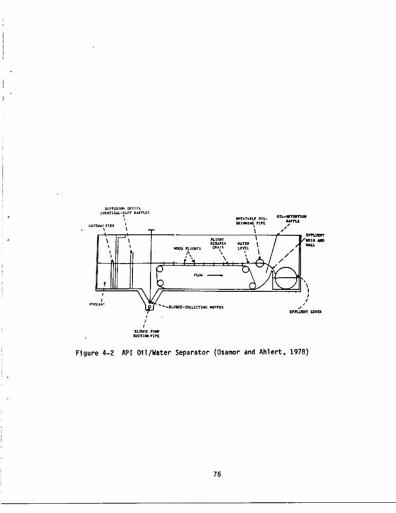
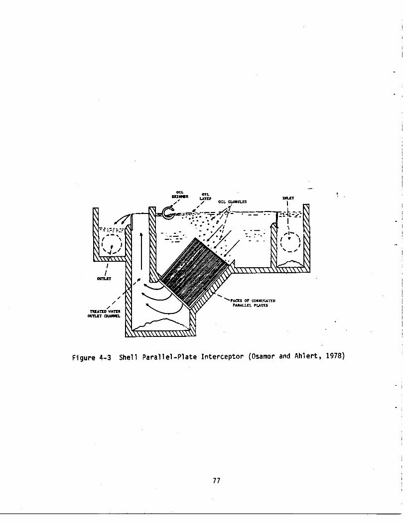
Osamor and Ahlert (1978) have prepared a detailed description of these

treatment methods . The most commonly used treatment methods are gravity

differential systems (which may also employ skimming and dissolved air flota-

tion) and filtration systems . The gravity differential systems provide the

bulk of oil/water separation using various types of systems . These systems

include : API oil/water separators ; circular separators ; plate separators

(PPI, CPI, Curved plate separators) ; and rotational separators (Centrifuges) .

The filtration systems vary in complexity from slow sand filters with uniform

or graded beds to membrane filters utilizing electrodialysis, reverse osmosis,

or ultrafiltration . The use of synthetics such as polyurethane is also

72

TABLE 4-1

SUMMARY OF POTENTIAL TREATMENT TECHNIQUES FOR REMOVAL OF OIL FROM WATER

TechniqueFreeoil

Oil-coated solids Unstabilizeddispersions

Stabilizeddispersion

MolecularlySettle-able

Neutrallybuoyant

Surface Solubilized

dissolvedPrimary Secondary Chemically charge

oil

oil

A . GravityDifferentialAPI XXX* XX XHydrogard XXX XX XCircular XXX XX XPPI XXX XX XXCPI XXX XX XX XFram-Akers XXX XXX XXX XXX XXCurved-plate

finger XXX XXX XX XX XGravi-Pak XXX XXX XXXCentrifuges XXX XXX XXXHydrocyclones XX XXXVortex XX XXDispersed air

flotation XXX XXX X XXDissolved air

flotation XXX XXX XX XXX XXVacuum desorption XXX XXX XX XXX XXElectrochemical X XX XX XXX

B . FiltrationGranular media XXX XXX XXX XX X XMultimedia XXX XXX XXX XXX XX XX

C . Coalescence/FiltrationFibrous media XXX XXX XXXCentrifuge XXX XXX XXXBimetallic XX XXX

J . Chromatography

K . SonicandUltrasonic

TABLE 4-1 (continued)

* X, poor separation ; XX, average separation ; XXX, excellent separation .

X

XXX

XXX

TechniqueFreeoil

Oil-coated solids Unstabilizeddispersions

Stabilizeddispersions

Solubilizedoil

Molecularlydissolved

oilSettle-able

Neutrallybuoyant

SurfacePrimary Secondary Chemically charge

D. MembraneElectrodia ysis XX XX XX XX XX X XReverse osmosis XXX XXX XXX XXX XXX XXX XXXUltrafiltration XXX XXX XXX XXX XXX XXX XX

E. AdsorptionCarbon synthetics XXX XXX XXX XXX XXX XXX

F . Electric andMagneticElectrophoretic X XXMagnetic XX

G . Thermal XX X

H . Coanda Effect X

I . Viscosity-Actuated X

receiving attention as a suitable filter medium (Canadian Plant and Process

Engineering Limited, 1972), although the use of adsorption and absorption

systems has been limited to the cleanup of oil spills .

Gravity differential separation is the oldest method for separating

oil/water mixtures . In general, oil/water mixtures will separate naturally

into two distinct layers of oil and water if allowed to stand undisturbed for

a sufficient period of time . The basic principle governing this technique is

Stoke's Law, which evaluates the rate of rise of oil globules in water based

upon density . Stoke's Law also applies to oil coated solids suspended in

water.

The rate of rise of an oil globule i s dependent to a large extent on the

particle size . For an appreciable separation to occur, within reasonable

residence times, the oil droplets and suspended solids must be large . As oil

globules rise to the surface, collisions occur, coalescence takes place, and a

floating oil film forms at the surface . Subsequent skimming removes the free

oil .

The most economical state-of-the:art methods in oil/water separation are

of the gravity type . These devices can handle large flow rates, have low

power requirements, and need minimum operator attention ; but processes are

slow, necessitating large equipment . Gravity separation is basic to almost

all oil/water separators .

Within the category of gravity separation, the three most common types

are : (1) the API oil/water separator ; (2) the shell parallel plate inter-

ceptor (PPI) and/ (3) the shell corrugated plate separator (CPI), as shown in

Figures 4-2 through 4-4. The PPI and CPI use tube settling, or a variation

thereof to reduce the size requirements of the overall device . Functionally,

all 3 separators perform in a similar manner .

75

DIFFUSION DEVICL(VERTICAL-SLOT RAFFLE)

?

I

ROTATARLF OIL-

OIL-WTDMON

GATEWAY PIER

I

SKIMMING PIPE1

.0

t

J

t

d

-SLUDGE-COLLECTING HOPPER

f

SLUDGE PUMPSUCTION PIPE

Figure 4-2 API Oil/Water Separator (Osamor and Ahlert, 1978)

76

I

OIL

OILSUMMER

LAYER

IRLETOIL GLOBULES

'

VWMIM

Figure 4-3 Shell Parallel-Plate Interceptor (Osamor and Ahlert, 1978)

77

IPACKS or PARALLEL1MCLiMED PLATES

SiiCT10K MUSEPot SLUOGE

Figure 4-4 Shell Corrugated Plate Interceptor (Osamor and Ahlert, 1978)

78

The performance of the gravity separators as represented by several

investigators (Osamor, et al, 1978) is presented on Tables 4-2 and 4-3 . The

lowest reported effluent concentrations are about 200 mg/1 . These separators

are generally used to provide initial or coarse separation, and are almost

universally employed as a preliminary unit process for oil removal to lower

concentrations .

The concept of gravitational separation between fluids of different

densities can be enhanced by the use of centrifuges . Centrifuges can produce

faster settling by generating forces of 1,000 to 5,000 times the gravity

force. To operate satisfactorily, they require a density difference between

the oil and water of at least 5%, and relatively high concentrations of oil

(1,000-60,000 mg/1) . The latter requirements makes their use unsuitable for

the relatively low oil concentrations found in urban runoff . The power,

operating, and maintenance requirements would also be unfavorable .

The gas flotation concept of gravity separation has been used for

oil/water separation . The flotation variations have employed : (1) dispersed

air (2) dissolved air, (3) vacuum desorption, and ; (4) electrochemical . The

successful operation of the flotation systems is based upon pilot studies, and

a fairly steady flow volume and flow characteristics .

Filtration through granular materials is one of the oldest methods for

separating oil/water mixtures . This technique is useful for removing sus-

pended matter and associated oil from oily wastewaters . It is best suited for

removing oil-coated solids that cause fouling in a coalescing device . Neu-

trally buoyant oil-coated solids that require infinite settling times can also

be removed . Filtration is becoming important in the petroleum industry

because of its capacity to reduce the concentration of oily suspended solids

79

TABLE 4-2 OIL AND SUSPENDED-SOLIDS REMOVAL IN GRAVITY-TYPE SEPARATORS(OSAMOR, 1978)

TABLE 4-3 ESTIMATED EFFLUENT QUALITY FROM PRIMARY OIL/WATER SEPARATIONPROCESSES (OSAMOR, 1978)

80

Oil content (ppm) Percent OilRemoval

Percent Suspended-Solids Removal TypeInfluent Effluent

300 40 87 - PPI

220 49 78 - API

108 20 82 - ci rcul ar

108 50 54 - circular

98 44 55 - API

100 40 60 - API

42 20 52 API

2000 746 63 33 API

1250 170 87 68 API

1400 270 81 35 API

Separators commerciallyavailable

Effluent oilconcentration

(mg/1)

API rectangular 50-75

Circular 50-75

Inland Steel--Hydrogard 50-75

Shell PPI 35-50

Finger-plate separator 35-50

Fram-Akers plate separator 40-100

Keene--Gravi-Pak 20

in production water that are passed to secondary and tertiary recovery opera-

tions .

The mechansims involved in filtration are very complex and little under-

stood . With deep granular filters of coarse material, removal is primarily

within the filter bed (commonly referred to as depth filtraton) . Some solids

may be removed by a process of interstitial straining, and oil may be removed

by adsorption on the bed material .

Filtration can be accomplished by two general techniques : layer and

membrane . The layer technique employs sand and other filtration media in a

thickness of 18 to 30 inches . Synthetic substrates such as polyurethane may

also prove useful . The membrane techniques are relatively new, and rely upon

processes such as reverse osmosis, ultra filtration ; and electrodialysis .

The performance of filtration in removing oil and grease is better than

that of gravity separation . Effluents with no visible oil and total concen-

trations of 10-20 mg/1 may typically occur. However, each filter bed has a

limited life, and performance drops as filter clogging occurs . Backwashing

will renew the filtration capacity. The use of gravity separation prior to

filtration may be desirable to decrease backwashing time and filter clogging .

ExistingPracticesinthePetroleumIndustry

A review of the oil and grease control practices in the petroleum

industry may provide useful information to possible control in urban runoff .

The response of the petroleum industry to emergency spills of oil has been

extensively documented (Oil Spill Conference Proceedings, API/EPA/USCG, 1971,

1973, 1975, 1977, 1979) . Oil spills do not occur (routinely) at known times

and locations . Many occur on the water, and land spills are not discussed .

The spill originates from an oil source, and the oil spreads and dissipates

81

away from the site . Rapid deployment to contain the spill is practiced to

minimize the area in which oil must be recovered from and to provide collec-

tion at the greatest concentration . Stormwater runoff, by comparison,

provides a relatively dilute concentration from many disperse sources . The

general steps in emergency oil spill response are :

1 . Stop oil flow from the source ;

2. Contain oil by use of floating booms, or natural wind or tidalaction ;

3 . recovery of contained oil and collect for later disposal ; and

4 . dispose or reuse oil .

Spill recovery techniques may be adaptable to stormwater oil and grease

control . Oil recovery during a spill may be made by use of skimmers, sorbents

or centrifugal separates .

Skimmers effectively separate oil and water under smooth water conditions

because a surface oil spill (with no mixing) provides conditions that are

rarely achieved in the best design of gravity separators . Skimmers may use a

floating weir and pump out oil from the surface . They tend to be very effec-

tive because oil exists in one form, floating oil, and at a thickness from

barely visible up to several inches thick . An appropriate skimming device

would be required with any gravity separation system.

Sorbents can be in the form of an endless belt of oleophilic material ;

rotating disks of oleophilic material ; and any floating material to which oil

will stick . The first two employ a squeegee or wiper effect to remove the

sorbed oil from the belt or disk, prior to readsorption of more oil . The

other types of sorbents are usually broadcast or spread over the oil surface,

and recoverd by either a mechanical or hand method . The sorbent material and

the attached oil is then either disposed or the oil is extracted (usually

physically) and the sorbent is reused .

82

The development of a distributed reusable-sorbent oil recovery system has

been accomplished by both the EPA and the Navy (API/EPA/USCG, 1977) . The two

applications of this technique were for identical conditions ; out at sea, with

conditions including large waves and currents . Ordinary skimmers and other

previously developed techniques were least successful under these conditions .

A critical component integral to the entire collection system in respect

to oil recovery or removal is the reusable sorbent . Both the EPA and the Navy

used an open cell industrial polyurethane foam . The other components of their

systems were a broadcaster, harvester, regenerator and storage units . Al-

though other adsorbents have been investigated, the polyurethane foam was

selected as the best choice under the reusable conditions . Some properties of

the foam that led to its selection are :

1 . high sorptive capacity, up to 80 times its weight ;

2. high recyclability (over 100 times) without loss of adsorbency ;

3 . high (90%) oil recovery by mechanical squeezing ; and,

4. low water retention during squeezing (only 3 times original weight) .

A limited tabulation of existing practices at Bay Area oil refineries and

terminals is presented below . The results are based upon a limited telephone

and mail survey .

Number of Locations (Total 15)

Oil/Grease Control Technique

3

API separators with or without flowequalization

2

Holding/oxidation ponds with skimmers

1

Total on-site containment andcontract removal by hauling

9

No response at present (either awaitingmail response or no informationavailable)

83

The separation of oil and water has been studied and practiced by manu-

facturing companies . The result has been the production of large number of

devices which utilize, among others, the treatment methods discussed above. A

limited approach was made to collect data on the presently manufactured

oil/water separation devices, and to critique, when possible, their operation .

The approach to tabulate manufacturers product literature used a three

part approach . The first approach was based upon a (April 1978) state-of-the

art survey of oil/water separation equipment (Osamor and Ahlert, 1978) . An

inquiry letter was sent to each manufacturer listed in the report . The second

approach utilized a manufacturer's listing for oil/water separation equipment

from a current issue of the Water Pollution Control Federation Journal . The

third, and last, approach was simply to follow up on advertisements, reader

service cards, information from other people, or any other promising source .

The overall results are adequate for the purposes of applying the results

of oil and grease removal in urban runoff . The results are not extremely

encouraging for a state-of-the-art review. As an example, from the first

approach :

90

letters were mailed out ;42

letters provided no response ;26

letters were returned as undeliverable ;6

letters received response, but no pertinent informa-tion ;

16

letters received a usable response

The second approach sent letters to 16 current manufacturers (WPCE

listing) resulting in :

1.6

letters were mailed out ;9

letters received usable responses ;2

letters received a non-pertinent response ;5

letters were unanswered

84

The third approach was used selectively to add information to the overall

listing . No specific accounting of the success of this approach is possible.

The tabulation by manufacturer is divided into 3 categories, gravity

separation, filtration, and other (miscellaneous), shown in Tables 4-4, 4-5,

and 4-6, respectively . The process equipment is tabulated by type, with the

least complex appearing first . No distinction was made between manufacturers

who provided custom design or standard prebuilt plants .

CentralizedStorage

The procedures reviewed above (excepting spill technology) demand water

flow at a controlled rate. A major difficulty in treating stormwater is that

precipitation occurs stochastically . Runoff events may be extreme, are highly

variable and are short and long lived . Technology capable of handling the

large range of runoff levels normally expected would have to be extremely

versatile, and would probably be very expensive and inefficient. Processes

generally maximize efficiencies at selected process rates . Storing runoff

during an event to enable treatment systems to proceed at relatively uniform

rates may provide a useful approach to maximizing oil and grease control

capabilities . Similarly, releasing runoff to the environment at a rate com-

mensurate with biologial assimilatory processes might ameliorate outfall

impacts .

There are various methods to accomplish this storage (Hannon, 1980 ;

Lynard et al 1980 ; Meadows, 1980, Poertner, 1974) . The most common method

would use water channelization into holding reservoirs or infiltration

basins . Large underground storage reservoirs may also be employed, as

currently being constructed for the city of Chicago . Some degradation of

pollutants would be expected during storage. Infiltration basins would

85

Manufactuer

EnvirexIndustrial Filter and Pump Co.Joy/Denver EquipmentPielkenroad

AFL IndustriesCE-NATCOEnvirex

AFL IndustriesBINABChiyoda Chemical Engineering

AFL IndustriesCE-NATCOFacet

Envirex

AFL IndustriesCE-NATCOECO-ResearchEnvi rexEnviroTechIndustrial Filter and Pump Co .Joy/Denver EquipmentPermutitWEMCO

ALFA Laval

TABLE 4-4 MANUFACTURERS OF GRAVITY SEPARATION EQUIPMENT

Equipment Description

ClarifiersClarifiersClarifiersClarifiers

SGI Gravity SeparatorAPI Clarifier/SeparatorAPI Clarifier/Separator

Plate Clarifiers (PPI, CPI, etc .)Plate Clarifiers (PPI, CPI, etc .)Plate Clarifiers (PPI, CPI, etc .)

Vertical Tube CoalescersCoalescence/ClarifierCoalescence/Clarifier

Flotation Separator

Dissolved Air FlotationDissolved Air FlotationDissovled Air FlotationDissolved Air FlotationDissolved Air FlotationDissolved Air FlotationDissolved Air FlotationDissolved Air FlotationDissolved Air Flotation

Centrifuges

86

Manufacturer

EnvirexMETPRONeptune Micro-Floc

BRNABChiyoda Chemical EngineersIndustrial Filter and Pump Co.

ContinentalMETPRO

CE-NATCOContinentalFacet

ROMICON

Manufacturer

Enquip

AFL IndustriesDouglas EngineersMetpro SystemsOil Recovery SystemsOil Skimmers, Inc .

Santina and Thompson

Cal gonCarborundumChiyoda Chemical Engineers

TABLE 4-5 MANUFACTURES OF FILTRATION EQUIPMENT

Equipment Description

Sand FiltersGravity FiltersMulti-Media Filters

Filters (artificial media)Filters (3 Types)Filters (many types)

Pressure FiltersPressure Filters

Coalescence/FiltersCoalescence/FiltersCoalescence/Filters

Ultra Filtration

TABLE 4-6 MANUFACTURERS OF OTHER nil-/WATER SEPARATION EQUIPMENT

Equipment Description

TSI Water Separation and Oil Recoverer

Skimmers (3 Types)Weir Skimmers (2 Sizes)Belt SkimmersSurface SkimmersOil Skimmer (Tube Type)

Swi rl Separators

Activated Carbon SystemsActivated Carbon SystemsActivated Carbon Systems

8 7

provide for elimination of stormwater at a relatively slow, controlled rate,

although offering the potential for pollutant entrapment in ground water .

Storage reservoirs could re-release water into the treatment system at a rate

suitable to the capabilities of the treatment facility or the biological

assimilatory capacity .

DecentralizedStorage

Storage could also be accomplished through the construction of numerous

catchment basins designed to hold storage from a limited area. Devices may be

built in to remove floatables or allow silt sedimentation . These basins could

be built uniformally throughout the watershed, or only placed in areas of

substantial oil and grease deposition .

The oil and grease traps would be most effective for floating, or easily

settled oil and attached solids . Hydraulic detention would be provided to

allow the oil/water separation to occur . This concept has been used at

several locations, noticeable at the Chicago Metro Bus Terminal (Industrial

Waste, 1980) and in King Co ., Washington (King County DPW, 1979) . The designs

employed increased hydraulic detention, and a down-turned outlet located below

the water surface to permit separation of floating oils . One design used

extensively in Washington State is shown in Figure 4-5 .

Although these devices received some use for control of oil, little

operating or performance data has been published . The concept is very

promising from the viewpoint of simplicity and cost, although a complete

analysis is not possible .

A modification of the basic oil/grease trap is available with a separate

compartment to separate oil (or other products) for subsequent recovery, as

shown in Figure 4-6 . Although the initial cost and complexity is greater than

88

f0 THAT MCSTRICTOR/ ESEPARATOR DEVICE isVISIBLE AT EDGE rOPENING AND DIRECT PENV OVER THE LADDERLOCKING LID REQUIRED)

SRESTRICTOR PLATEAPPROPRIATELYIZED ORIFICE CUTN PLATE. NOT RE-WIRED IF SYSTEMIS FOR POLLUTION

CONTROL ONLY . .-

CATCH BASIN

Figure 4-5 Flow Restrictor/Oil Separator Control Device/Catch Basin(After King County, DPN, 1979)

89

-GRATE ELEVATION

,OVERFLOW ELEVATION-SET TO PROVIDE RE-

QUIRED DETENTION ANDADEQUATE OIL SEPARA-TION PROTECTION

the simple grease traps, the potential exits to provide a revenue return to

pay for capital and maintenance costs .

Other devices may hold promise as a method for oil and grease removal,

although actual practice has not been demonstrated . A membrane device used to

stop rainflow inflow to a sanitary sewer (Hannon, 1980), could be modified

with oil absorbent materials to operate as an oil removal device as shown in

Figure 4-7 . Hydraulic considerations and maintenance requirements would be

.important design considerations .

Biodegradation

The degradation of oil and grease in cultivated soil has been well

documented (Francke and Clark, 1974 ; Kincannon, 1972), although at hydrocarbon

concentrations greater than ordinarily found in urban runoff . Some organisms

important to degradation have been identified as Pseudonomas putida and

Flavobacterium by McKenna and Heath (1976), Pseudomonas, Micrococcus and

Acinetobactor by Ward and Brock (1975) and Pseudomonas, Flavobacterian,

Nocardie, Corynebacterium and Arthsobactor by Kincannon (1972) . Dominant

general responsible for hydrocarbon oxidation in soils have also been reported

by Jones and Edington (1968) . Techniques utilizing biological degradation

processes warrant attention as possible methods of limiting oil and grease

loading from runoff .

A major difficulty of assessing the practicality of using soil and water

bacteria as a primary component of oil and grease treatment is that little

work can be found identifying decomposition rates in systems other than soil

cultivation or spills . Important conditions limiting or regulating the rate

of microbial decomposition include dissolved oxygen availability (Delaune et c

al, 1979) nitrogen and phosphorus availability (Atlas and Bartha, 1971 ;

90

WATER OR ow

trl :WATER'

;SUMP~0 . 1 1

WATERSEPARATION CHAMBER

Figure 4-6 TSI Gravity Separator (Patented)

91

Figure 4-7 Proposed Oil Adsorbent Device for Manhole (Hannon, 1980)

92

FILL BAG WITH OIL

ADSORBENT MATERIAL

Kincannon, 1972), temperature (Adhearns et al, 1976) salinity (Brown et al,

1970) and substrate acclimation (Brown et al, 1969) . It is probable that in

an ordinary flood control channel experiencing rapid flows over confined

areas, there is little opportunity for degradation . However, if flow were

dispersed and retained in a marsh or wetlands, increased degradation might be

facilitated by the greater hydraulic retention and soil/water interface.

The use of a marsh/wetland for removal of oil and grease from storm-water

runoff has not been undertaken, however, investigations have occurred to

measure the effects of oil spills (Baker, 1971 ; Burk, 1976 ; Cowell, 1969 ;

Cowell et al, 1969 ; Delaune et al, 1979 ; Hunter et al, 1970) . In general

terms, the biological (plant) reaction to large concentrations of oil has

varied from minor damage to death . The immediate species reaction is usually

overcome by the next season's growth, although a small number of species is

much slower to recover . No recommendations can be made as to a controlled use

of a wetland for oil and grease removal . At best, a conservative approach

would be warranted, and the availability of an alternative control method

would be prudent .

Other possible methods of promoting biological degradation coincide with

storage mechanisms discussed above . If stormwater were used in greenbelts or

lakes, biological processes would be expected to remove some of the hydro-

carbons . However, degradation rates are not known in these situations, and

care would be needed to ensure that loading did not overwhelm degradation

capacity to result in surface scumming . Similarly, infiltration basins might

eliminate some oil and grease, but loading capacity would have to be carefully

evaluated .

A system of small, localized greenbelts surrounding areas . of heavy oil

and grease deposition might offer a further method of promoting biodegrada-

93

tion . An example system would be a greenbelt surrounding a parking lot .

Periodic cleaning or washing of hydrocarbon deposits into these green areas

might eliminate much of the potential for subsequent pollution . Degradation

rates in the greenbelts would have to be determined in order to ensure against

overloading the system . However periodic soil cultivation, increasing biolog-

ical degradation and loading capacity, may be economically feasible in these

limited greenbelt areas .

Outfal1

The final possibility for runoff treatment prior to ultimate disposal is

at the outfall . A possible, if expensive, treatment alternative would use one

of the methodologies reviewed in the above discussion of petroleum technolo-

gies . A treatment alternative at the outfall would probably rely on some

upstream storage to maintain flow at a sustained level to enable efficient

treatment .

The location of the outfall probably is important to the effects of oil

and grease to the receiving body . A high level of productivity in most bodies

of water occurs in the littoral or neritic zones, perhaps presenting the

greatest opportunity for detrimental effects to occur from stormwater runoff

(Odum, 1971 ; Wetzel, 1975) . Although the threshold levels of oil and grease

are not formally established, dilution remains a possible treatment alterna-

tive . If outlet structures are located away from sensitive zones, in open

water, subsequent dilution and flushing may provide an effective solution to

oil and grease pollution in runoff. However, care needs to be taken in siting

outlet structures and evaluating pollutant pathways to ensure that any pollu-

tion effects are actually lost or reduced to the environment, rather than

spatially or temporally altered .

94

Dispersion of oil and grease could be promoted through the use of syn-

thetic dispersants . Ideally, sufficient dilution of pollutants may maintain

hydrocarbons at sub-threshold levels at any particular location while increas-

ing the surface area that bacteria may use to initiate degradation . Doe et al

(1978) prepared a bibliography describing some of the oil spill dispersants .

However, the use of dispersants also presents possible problems . Dispersing

oil and grease may simply alter or increase the area to be affected . Studies

indicate that dispersants may be toxic (Lonning and Falk-Persen, 1978 ; Heldal

et al, 1978) ; effects have been shown in concentrations as low as 1 ppm.

Ventallo (1975) reported that detergents, which may be used as dispersants,

can reduce oil degradation due to a bacterial preference for detergent de-

gradation . Unfortunately, it is often difficult to obtain the chemical make-

up of dispersants from the manufacturers, aggravating the task of determining

toxicity and biodegradability. Certainly, the use of dispersants needs a

critical evaluation prior to any treatment application .

No Control

A variety of possible mitigation measures to reduce or eliminate oil and

grease in stormwater have been presented above. Many of these measures are

expensive and require sophisticated technology . Other measures discussed are

less demanding technologically, but require investments in land or changes in

life style . In evaluating between oil and grease control alternatives,

factors suchs as costs, social impact and effectiveness of control should be

considered . However, the relative value of oil and grease control in runoff

should also be considered in relation to the inputs required for the control .

Little information is available on the effects of oil and grease at the

normal concentrations found in stormwater . However, this information is vital

95

if rational decisions are to be made concerning the degree of effort warranted

hydrocarbon stormwater runoff control .

Other deleterious materials besides oil and grease such as pesticides,

herbicides, nutrients, suspended solids and material with a high biochemical

oxygen demand may also be found in stormwaters . Overall runoff quality might

improve by diverting resources from oil and grease control into the treatment

of other pollutants . Any evaluation of the implementation of oil and grease

control techniques should also consider control effects on other pollutants .

Additional work needs to be done concerning these other possible pollutants,

as well as determining the effects of oil and grease in stormwater, to deter-

mine the optimum resource allocation for enhancing environmental quality .

Summary

This section has summarized existing experiences with a variety of types

of oil/water separators . Most of the techniques discussed are used primarily

for separation of oil/water mixtures produced by manufacturing processes . The

optimal treatment method for urban stormwater runoff may be quite different

than the optimal technique for oily process wastewater . Further development

work is required before the selection of the best technique can be made with

assurance.

96

CHAPTER 5

DATA COLLECTION AND ANALYSIS

Objectives

A field sampling program was conducted during winter 1980-1981 to examine

oil and grease concentrations in urban stormwater runoff from a demonstration

watershed in Richmond, California . Richmond contains a variety of types of

light-to-heavy industry and is located north of Oakland . It is typical of many

small towns and cities and is not a "bedroom" suburb of Oakland or San

Francisco . Five stormwater sampling stations representative of commercial,

industrial, and residential areas were initially selected for evaluation of

oil and grease from various land uses . Runoff from a total of seven storm

events was sampled .

The sampling program encompassed three major goals :

1 . Determination of oil and grease concentrations and load factors

corresponding to various land uses .

2. Quantification of the relationships between oil and grease concentra-

tion and precipitation/runoff patterns .

3 Chemical characterization of oil and grease runoff from various land

uses, with the objective of determining the source of the oil and

grease .

SiteDescription

The study area is a 2 .5 square mile area within the city of Richmond .

The watershed contains a mixture of commercial, industrial, and urban residen-

tial land uses . Single family residential dwellings comprise approximately 70

9 7

percent of the total watershed area . Table 5-1 lists and describes the

various land uses in the study area . The locations of the selected sampling

stations are shown in Figure 5-1 .

Eight land use categories were developed for the study area . These were

developed from aerial photographs and were based upon similarities to the

sampling locations .

1 . Undeveloped . Open areas, grass areas, football fields .

2 . Industrial property and parking.

Total industrial area including

parking areas, paved or dirt, and buildings . (Represented by Safeway

Distribution Center : Station 2) .

3 . Large-scale commercial property and parking . Parking lots, paved or

dirt, and buildings . Also includes parking lots in non-commercial

areas where automobiles are predominant, such as schools . (Repre-

sented by Montgomery Wards Lot : Station 3) .

4 . Small-scale commercial property including the associated parking lots

and commercial streets .

Street areas including buildings with small

scale commercial and industrial businesses dealing with the public,

i .e. where small parking lots and automobiles predominate . (Repre-

sented by San Pablo Avenue : Station 4) .

5 . Single-family residential . (Represented by Station 5 .

6 . Multi-family residential .

7. Freeways, trains and BART tracks .

8 . Impervious non-auto .

Tennis courts, playgrounds, and other areas

which appear to be impervious, not identifiable in other categories .

98

TABLE 5-1

LAND USE IN THE RICHMOND WATERSHED

Total Calculated Land Area - 2 .541 square miles

99

Land Uses % of total area

1 . Undeveloped 5 .2

2. Industrial parking and property 4 .3

3 . Large-scale commercial parkingand property

6 .0

4 . Small-scale commercial and industrialparking and property

5 .8

5. Single family residential 70.6

6. Multi-family residential 2 .1

7 . Freeways, trains and BART 3 .6

8 . Impervious non-auto 2 .4

Figure 5-1 Location of Richmond Field Sampling Stations

100

iI0

3

rKC'Wrri

innerHarborBean

Richmond

Inner

Harbor

Sample StationDescription

Five sampling stations were selected to represent the following land use

categories : mouth of the watershed (station 1) ; industrial parking and

property (station 2 - Safeway Distribution Center) ; large-scale commercial

property and parking (station 3 - Montgomery Wards parking lot) ; small-scale

commercial property and parking (station 4 - service station on Major Street) ;

residential (station 5) . Although these stations were generally believed to

be representative of a single land use category, often the entire station area

represented a composite of two or more land use types . Descriptions of the

individual sampling stations and the representative land uses are provided in

Table 5-2. Land use and station areas were determined from aerial photo-

graphs . Station drainages were determined from Richmond storm flow maps which

illustrate water drainage direction and station drainage boundaries . Station

2 (Safeway distribution Center) and Station 3 (parking lot) were assumed to

drain only one-half the total measured area ; two drains were assumed for each

of these large areas . The sampling locations and land uses are described

below.

Station 1 - Mouth of the Watershed : Station 1 was located at the mouth

of the demonstration watershed, near the intersection of 32nd Street and

Griffin Avenue . At this point, the entire study area stormwater runoff flows

in a concrete trapezoidal drainage channel to San Francisco Bay . Sampling at

this station represents a composite of runoff from all contributing urban land

uses in the watershed .

Station 2 - Safeway Distribution. Center : Station 2 was located near

station 1, but outside of the demonstration watershed . This station was

selected because it was thought to represent a large portion of land uses

within the watershed, and for its convenience of sampling and monitoring . The

101

# measured as distance to station 1

TABLE 5-2 . DESCRIPTION OF SAMPLING STATIONS

STATION SITE DESCRIPTION AREA LAND USES

DRAINAGE AREA (ft 2)

APPROX . DISTANCETO MOUTH OFBASIN (ft)#

ELEVATION ABOVESEA LEVEL (ft)

1 Mouth of Watershed Composite of all 7 .08 x 107 0 12uses in the watershed

2 Safeway Distribu-tion Center

77% industrialproperty and parking ;

1 .17 x 106 2,000 10

23% impervious non-auto

3 Parking Lotcommercial propertyand parking

100% large-scale 2 .92 x 104 6,250 60

4 Service Station 70% residential 8 .71 x 105 9,800 10330% small-scalecommercial propertyand parking

5 Upstream Resi-dential Area

95% residential5% undeveloped

5 .7 x 106 10,500 98

station was at the collection point for surface runoff from the Safeway

Distribution Center, which is located adjacent to the primary watershed . The

established sampling point was at the outfall of a 30" concrete culvert which

crosses east to west beneath S . 27th Street, north of the intersection with

Pierson Avenue . Sampling at this location is representative of an industrial

site with heavy truck traffic . (77% industrial parking ; 23% impervious non-

auto, i .e . roof) .

Station 3 - Montgomery Wards Parking Lot : Station 3 was the drainage

outlet for the Montgomery Wards front parking lot near the corner of McDonald

Avenue and 44th Street . In this area, runoff from the asphalt parking surface

is directed to the east side of the lot where it is funneled through a

tapered, sloping concrete apron leading to a drop inlet into the underground

storm sewer. The sampling was at the tapered apron section . This sampling

site was representative of off-street automobile traffic and parking in the

commercial district (100% large-scale commercial parking and property) .

Station 4 - San Pablo Avenue : Station 4 was located at a curb and gutter

section In front of the Regal Service Station on the east side of San Pablo

Avenue approximately 100 feet south of the intersection with Garvin Avenue .

Runoff in this area is from primarily commercial land use with some contribu-

tion from single family residences and apartments . Drainage includes runoff

from three service stations and is carried solely in street gutters . No

underground sewers exist in this section . Sampling at this station represents

heavy automobile traffic, curb-side and off-street parking and service station

contributions along a major commercial artery . (70% residential ; 30% small-

scale commercial) .

Station 5 - Upstream Residential Area :

Station 5 was located in the

residential upper portion of the watershed near the intersection of Solano

103

Avenue and Amador Street . The sampling site was an open, unlined drainage

channel on the upstream (southeast) side of Amador Street . Sampling at this

point represents contributions from a well-established urban residential area

in moderate to steeply sloping terrain . (95% residential ; 5% undeveloped) .

StormCharacterization

Runoff from a total of seven storm events was sampled during the 1980-81

winter season . The initial program objective was to sample six storms having

rainfall intensities of at least 0.2" within the first six hours of the storm ;

the rationale was to focus on storms having sufficient "washoff" potential .

An additional stipulation was that at least five of the six storms be preceded

by a minimum of three consecutive days without rainfall in order to allow an

interval for street surface accumulation of contaminants between samplings .

Because of an abnormally dry winter season, it was not possible to adhere

strictly to these target sampling guidelines . Table 5-3 provides a summary of

date of the storm, days since previous storm, storm duration, and total rain-

fall for each of the seven storms . The storm events varied widely in their

characteristics .

Experimental Design

SampleCollection

One liter grab samples were collected at each station with an intended

frequency the following time intervals after the beginning of the storm until

the end of the storm : 0.5 hour, 1 hour, 1 .5 hours, 2 hours, 3 hours, 4 hours,

6 hours, 9 hours, 13 hours, 18 hours . This schedule was intended to provide

intensive sampling during the initial runoff period for each storm decreasing

the sampling frequency as the storm continued and eventually dissipated . Some

modification was occasionally made up this schedule due to field conditions

104

105

TABLE 5-3 SUMMARY OF RAINFALL DATA FOR EACH STORM EVENT

STORM DATEDAYS SINCE

PREVIOUS STORMSTORM

DURATION (hours)TOTAL

RAINFALL (in .)

1 12/3/80 11 15 .5 2 .01

2 12/21/80 18 4 .5 0.33

3 1/17/81 1 4 .5 0 .07

4 1/20/81 1 1 0 .4

5 2/13/81 5 3 .5 0 .35

6 3/4/81 4 6 0.24

7 3/18/81 3 7 0 .53

and availability of personnel . All samples were collected directly in one

liter glass containers which were pre-washed with freon and capped in accor-

dance with standard methods for oil and grease analysis . Sampling locations

were carefully selected and prepared to allow for collection at a point of

turbulent flow or free discharge . This procedure was necessary to assure that

samples were representative of a fully mixed water column . Specific proce-

dures followed at each sampling station were as follows :

Station 1 - Samples were obtained in a highly turbulent zone at the

double-culvert entrance to the trapezoidal open channel at the mouth

of the watershed .

Samples were obtained directly by securing the

glass sample bottles to a holder attached to the end of an extendable

aluminum pole and submerging the bottle, throat upstream, into the

most turbulent section of flow. This procedure proved effective under

all flow conditions .

• Station 2 - Samples were collected from runoff passing over a sharp-

crested V-notch weir fixed at the end of the 30" discharge culvert .

Integrated samples were obtained directly in the glass sample con-

tainer by passing the bottles laterally and vertically through the

discharge. This procedure proved to be effective for all flow condi-

tions .

• Station 3 - Samples were obtained by channeling runoff from the

parking lot over a sharp-crested V-notch (low flow) and 30" rectan-

gular (high flow) weir at the point of entry to the storm sewer. A

complete cross-section of the runof flow was readily obtained by

capturing the weir overflow directly in the glass sample containers .

1 06

• Station 4 - Samples at this station were taken directly from the

gutter flow and, in most cases, necessitated the use of two sample

bottles to obtain one full liter of runoff water. This was accom-

plished by filling two containers halfway or, in instances of low

flow, collecting the small volumes in one container and transferring

repeatedly to a second bottle . In all cases, both sample bottles

were submitted to the laboratory for extraction and analysis as a

single sample. The collection point was located in a rutted asphalt

section at the end of a smooth, uniform section of cohcrete gutter

and apron . The transition from a smooth to a rough bottom surface

created turbulent mixing conditions needed for sampling . This site

posed difficulties for sample collection only during extremely low

flow conditions, usually toward the end of a storm . Obtaining

samples during these times required the use of a sandbag to detain

the flow. On two occasions, samples had to be obtained 50 feet

"downgutter" where the flow passed through a pothole .

• Station 5 - Samples of stormwater runoff,were obtained at this site

directly from the flow passing over a sharp-crested 50" rectangular

weir installed in the open drainage channel . The glass sample

bottles were secured to a holder at the end of an extendable aluminum

rod and passed across the weir discharge to obtain an integrated

runoff sample. This procedure proved to be effective under all flow

conditions .

Duplicates of each routine sample were taken at all stations for all

sampling times during storm 3 . All procedures for sample collection, pre-

servation, labelling and handling were identical to those for the routine

107

samples . Each one liter sample was preserved in the field immediately follow-

ing its collection with five milliliters of concentrated hydrochloric acid

solution (diluted 1 :1 with distilled water) .

Collected samples were retained in the field at each sampling station or

in vehicles used by the field crew until the conclusion of the storm . Samples

were then stored at RAMLIT Associates offices until delivery to the analytical

laboratory. In all cases, samples were delivered to the laboratory within 24-

30 hours following their collection in the field .

MeasurementofOilandGreaseConcentration

The level of oil and grease in the stormwater samples was measured using

the Infrared Spectrophotometric Method (Method 413 .2) described in the EPA

report, "Methods for Chemical Analysis of Water and Wastes" (EPA, 1979) . It

is virtually identical to the Partition-Infrared method described in Standard

Methods (1975) . According to this method, the sample is acidified to a low pH

(<2) and extracted with fluorocarbon-113 (1,1,2-trichlor-1, 2,2-trifluo-

rethane, or Freon) . The oil and grease level Is then determined by comparison

of the infrared absorbance of the sample extract with standards . All of the

organic material extracted from aqueous solution or suspension by the Freon is

termed "oil and grease" . The material dissolved into the Freon generally

includes relatively non-volatile hydrocarbons, vegetable oils, animal fats,

soaps, waxes, esters, and fatty acids (Sawyer and McCarty, 1978 ; Standard

Methods, 1975 ; EPA, 1979) . Additional compounds which may be extracted

include elemental sulfur and certain organic dyes (Standard Methods, 1975) .

Two other methods of measuring oil and grease are described in Standard

Methods and are commonly applied to water and wastewater . The two methods,

"Partition-Gravimetric Method" and "Soxhlet Extraction Method", involve

108

solvent extraction, heating to evaporate the solvent, and weighing of the

residue to determine the oil and grease content of the sample . The first

method calls for heating the solvent-extracted sample to 70°C, and the second

method calls for heating it to 103°C . This solvent removal step would also

tend to volatize any short-chain hydrocarbons and simple aromatics present in

the sample . As a result, petroleum fuels from gasoline through No . 2 fuel

oils would be completely or partially lost (EPA, 1979) . The infrared proce-

dure used in this study does not call for a heating step . Thus, it can

measure most of the light petroleum fuels which may be present in the sam-

ples. Nonetheless, loss of about half of any gasoline present during the

extraction manipulation can be expected (EPA, 1979) .

In this study, the primary advantage of the Infrared Method is its

superior performance in measuring low levels of oil and grease . Standard

Methods recommends its use when measuring oil and grease levels less than 10

mg/i because gravimetric methods do not provide the needed precision for

accurate work . The EPA indicates that the Infrared Method is applicable to

samples with from 0.2 to 1000 mg/1 of extractable material, whereas the

gravimetric measurement (combined with the separatory funnel extraction) is

applicable to samples with a higher beginning-point range, 5 to 1000 mg/1 . In

addition, infrared measurements of oil and grease are not susceptible to

interferences such as sulfur (EPA, 1979) .

Rainfall Measurements

Rainfall data were collected for the duration of the sampling program at

an established weather station located within the watershed at the Richmond

City Hall . The rain gauge, operated and serviced by city of Richmond engi-

neering personnel, was an automatic tipping bucket gauge with recorder .

109

In addition, non-recording rain gauges were installed at stations 1 and 4

for observation by field personnel during the course of sampling each storm

event . These gauges, while much less precise than the recording gauge at the

City Hall, provided immediate information regarding the intensities and total

amounts of rainfall which characterized each storm . It was initially antici-

pated that such immediate information might be needed for field decisions

concerning termination of sampling for individual storm events . However,

other field observations of rainfall and runoff conditions proved to be more

effective indicators .

Flow Measurements

At the time each sample was collected, runoff flow rate was also esti-

mated . Methods were established individually for each station and included

the use of sharp-crested weirs, area-velocity measurements, and application of

Manning's formula for open channel flow . Details of the procedure followed at

each sampling . station are described below .

Station 1 Measurement of stream flow at station 1 was made under the

assumption of steady, uniform flow in the trapezoidal channel . Figure 5-2

illustrates the channel cross-section at station 1 . Dimensions of the channel

were obtained from "as-built" plans provided by the City of Richmond Public

Works Department . A staff gauge was installed on the 1-1 slope of the east

side of the channel at a point approximately 500 feet downstream of the

double-culvert entrance to the open channel . This point was judged to be free

of excessive turbulence and conveniently located adjacent to an access gate

and a street lamp . No apparent inflow, other than direct rainfall, enters the

channel between the sampling point and the flow measurement point .

110

Figure 5-2 Channel Cross-Section at Station 1

"NOTCH CONSTNUCTION JOINT

O" AGGREGATE Oa ;E

I

The staff gauge installed was a Leopold-Stevens Style "C" . It was porce-

lain-enamel, white with black markings 2 1/p' wide, 1/8" thick, with divisions

to .01 feet .

Initially it was placed on a vertical standard installed mid-

channel . channel. Experience during the first storm showed that this positioning led

to excessive turbulence and debris accumulation, thus

obstructing stage readings . The gauge was moved to the slope position follow-

ing the first storm and remained there for the remaining six storm events .

Volumetric flow rates were estimated by application of Manning's formula

for open channel flow. Calculations were made as shown by the example below .

K' b8/3 ~/2Q

N

Where : Q = flow

K' = function of channel dimensions and stage height (D)**b = channel width = 0.00386n = Manning's n = .014***

As an example, flow for a 2.0" is calculated as follows :

Stage height

0

2.0

25b = * = .

K' = .15(5 .3)

Q =( .15) (8 .0)14 ( .00386)1/2 (5 .4)

*

King and Brater Handbook of Hydraulics, 5th Edition, McGraw-Hill, 1963,p . 7-14 .

**

Ibid ., pp . 7-14, 7-38 .*** Ibid, p . 7-17 .

1 1 2

Manning's Formula*(5.1)

(5 .2)

Q = 170CFS (5 .5)

Station 2 Flow measurement at station 2 was facilitated by the fabrica-

tion and installation of a sharp-crested 90° V-notch weir at the outfall of

the 30" culvert which drains the Safeway trucking area . The weir proved to be

particularly effective in allowing accurate measurement of low flow conditions

and in minimizing backwater interference from the tidal slough into which the

culvert discharges . The discharge over the weir was in a free discharge

condition over 80% of the time . The combination of rainfall intensity and

tidal conditions at this station created partially submerged discharge condi-

tions during eight flow readings at storms #1 and #7 . Accurate flow measure-

ments were not possible in all of these instances . During one measurement of

storm #1, the backwater and high flow conditions totally submerged the weir

resulting in a less accurate flow estimation .

Under conditions of partial submergence, upstream and downstream stage

measurements were utilized. The submerged flow (0) was computed as a fraction

of the corresponding free discharge (Q 1 ) for the same upstream stage height

(Hu ) .* This was done with the use of empirical curves of0

vs Hu where Hu1

dequals upstream stage and H d equals downstream stage height .

Field measurements of the stage height upstream of the V-notch weir were

made by a reading staff gauge, consisting of an engineer's rule, permanently

positioned within the culvert . During periods of submergence, measurements of

backwater conditions were also made from a fixed reference point . Flow rates

*

King and Brater, p . 5-16

113

were calculated according to the following empirical formula for sharp-

crested, 900 V-notch weirs :

Q = (2.5) (H2 .5)*

*

(5.6)

Where : H = upstream stage height

Station 3 Runoff flow at station 3 was measured using two portable

sharp-crested weirs installed at the time of sampling . The weirs were fabri-

cated to fit snugly within the tapered apron at the prescribed sampling

location but were positioned so that they could be readily secured in place at

the beginning of a storm event and removed at its conclusion to minimize

changes of vandalism or interference with runoff and activities within the

parking lot .

A 90° V-notch weir was used to obtain accurate readings of low flow

conditions . A 30" rectangular weir was substituted during periods of intense

rainfall and runoff . For each weir, a staff gauge, consisting of an engi-

neer's rule, was fixed in place with each weir installation . The gauge was

positioned to allow consistent measurement of water level height at a point

upstream and away from the influence of the weir overflow crest .

Flow calculations were made using standard weir formulas and coeffi-

cients . The 90° V-notch weir is shown in Figure 5-3, and flow calculations

were made as follows :

0 = (2 .5)(H)2 .5**

Where :

Q = flow

*

King and Brater, p . 5-16** King and Brater, p . 5-14

Ce = discharge coefficient - a function of L, b, H, P

1 1 4

(5.7)

Figure 5-3 Typical 90° V-Notch Weir

115

Le

He

= Weir length (30") + correction for contraction (L/b)

= Upstream head (h) + correction factor of .003' for

viscosity and surface tension

Station 4 Runoff flow at station #4 was estimated by measuring cross-

sectional area (A) and surface flow velocity (V) for the range of conditions

encountered during the sampling program . Repeated velocity measurements were

taken for a variety of conditions along an established 20' section of uniform

concrete gutter and apron at the sampling site . A small bark chip was used as

a float to obtain surface velocity . The cross sectional area for various flow

depths (curb height) was determined from a cardboard template scribed for the

gutter at the sampling point . The flow depth, measured against the curb, was

determined at the time each sample was obtained . From these measurements,

flow (Q) was computed as follows :

Q=0.85*V*A

(5.8)

The values of flow for all field measurements of velocity (and computed

area) were plotted against curb height values in Figure 5-4 . This forms the

stage-discharge rating curve from which flows were estimated for all field

measurements of curb height .

Station 5 Measurement of stream flow at station 5 was accomplished using

a sharp-crested 50" rectangular weir permanently installed in the unlined open

channel . The weir and supporting structure was constructed of rough-sawn

redwood, and spanned the channel at the upstream edge of an existing concrete

culvert and apron into which the open channel streamflow discharges . A 4"

strip of 1/16" flat steel was fastened to the upstream side of the weir to

form a sharp-crest .

116

;s

.10

.or

20V

m .i5jV

.m

a.s 1O P.

SA

2-5

FLOW RM (cf%)

3.0 ;S 'A 4f

Figure 5-4 Rating Curve for Station 5

so (r0 LS TO

Approximately 10 feet upstream of the weir installation, a Leopold-

Stevens stule staff gauge, identical to that used at station 1, was mounted on

a stationary vertical 2" x 4" . This provided measurement of upstream stage

height in a quiescent section of the channel . Stage height readings were made

and recorded, . flow rates were subsequently computed according to the empirical

formula for rectangular weirs as previously described for station 3 and

according to the dimensions shown in Figure 5-5 .

Settlability of Oil and Grease

Two settling column tests were performed to assess the feasibility of

gravity separation as a runoff treatment technique . Samples from station 1

(mouth of the watershed) and station 3 (Montgomery Wards Parking Lot) were

taken during the fifth storm included in the study (February 13, 1981) .

Approximately 45 liters of water were allowed to settle in a glass column with

an internal diameter of approximately 15 cm and a height of about 1 .8 m .

Three hundred fifty ml samples were withdrawn from each of three ports at 1,

2, 5, 10 and 30 minutes after mixing with a plunger mechanism . Sampling ports

were located at approximately the mid-depth of the column, at about 30 cm

below the water surface and at about 30 cm above the bottom of the column .

After the 30 minute sample was taken approximately 1 liter was withdrawn from

the surface for analysis . The remainder of the sample was then siphoned, with

the bottom liter subsequently analyzed for oil and grease . Sample delivery

containers, plunger and column were rinsed with freon to collect organics

absorbed to surfaces . All samples were analyzed for oil and grease following

the Infrared Spectrophotometric Method described above .

118

HT

P=6"J/

Figure 5-5 Typical Rectangular Weir

i1 1 9

CharacterizationofOil andGreasein RichmondWatershedRunoff

As was described earlier in this chapter, oil and grease were removed

from the water samples by fresh extraction . Selected extracts were stripped

of the fresh solvent by heating on a steam bath and a nitrogen stream .

Nitrogen was used instead of air owing to the purity of nitrogen available .

The residue was redissolved in 100-200 microliters of pesticide quality

dichloremethane (CH2C1 2) . After mixing, 1 microliter aliquots of the prepared

samples were analyzed by gas chromatography .

A Tractor Model 760 gas chromatograph with a flame ionization detector

(FID) was used for this study . Instrumental parameters and column conditions

were as follows :

Injector :

300°COven :

50°C initial for 2 min ., then rising 8°C/minto 350°C

Column :

6' glass x 1/4' O .D .10% SP-2100 on 100/120 Supelcoport

As reference standards, n-decane, n-hexadecane, anthracene, C 24 , and C 32 were

used (Fitch, 1981) .

Data Analysis

Data collected from the field sampling program were analyzed using a

statistical analysis program, Statistical Analysis System (SAS, 1979) .

Intermediate variables were calculated and manipulated with FORTRAN . A

variety of types of statistical analysis were used, including analysis of

variance . The following set of variables were used to describe the storm and

runoff characteristics .

1) Oil and grease concentration (OG1, mg/1)

2) Total oil and grease mass runoff per storm (TMASS, lb)

3) Instantaneous runoff flow (FLOW)

4) Total runoff flow per storm (TFLOW, 10 6 gal)

120

5) Rainfall rate (RRAIN, 10-2 in/hr)

6) Total storm rainfall (TRAIN, in .)

7) Mass flow rate of oil and grease (RMASS, lb/day)

8) Days between storms (DBS, days)

9) Time since storm beginning (TSSB, hours)

10) Station number (STANO)

11) Storm number (STONO)

12) Sample number (SAMNO)

Each of the parameters was determined directly, with the exception of

total mass and total runoff flow volume, flows, which are defined as follows :

TFLOW = Jte•

FLOW dt

TMASS = fte•

RMASS dt

where : to = time of storm flow ending .

To approximate the integration, modified-Euler (often call trapezoidal)

integration method was used, as follows :

nTFLOW = ~= (FLOWi+1+ FLOW1 ) * (to+1 - ti)/2 (5 .11)

0

nTMASS = I (FLOWi+1 * OG1in + FLOWi+1 * OG1 1+1 ) * (ti+1 - ti)/2 (5 .12)

1=0

where n = number of sample points

i = sample point number .

The zeroth sample was always treated as the flow rate and oil and grease

concentration at the instant of storm beginning, which was always zero . In

121

the case of storm 1, the first sample was not taken until approximately six

hours into the storm, which could result in considerable error .

RawDataandSimpleStatistics

The raw data for the entire series of storms and sites is tabulated in

Appendix A. There are approximately 290 observations of each variable .

Consequently, the raw data are too lengthy to include in the text ; however,

the simple statistics (mean, standard deviation, standard error, and number of

observations) are listed in Tables 5-4 to 5-20 .

Runoff Flow

Mean values of instantaneous runoff flow measured at each station for

each storm are listed in Table 5-4 . These results reflect the average of

observations at regular intervals during the storm . Total runoff flow volume

for each storm as monitored at each station is presented in Table 5-5 . Runoff

at each station is related to the area of the drainage basin which feeds the

sampling point .

Runoff for each storm can roughly be related to rainfall . Contrary to

expectations, however, the runoff-rainfall ratio or runoff coefficient (K

value), varied considerably between storms . Storms 1 and 7 had quite high K

values . In spite of the fact that a larger storm is expected to have a

somewhat higher runoff-rainfall ratio, the K value for storm 1 at station 3

appears unreasonable at first glance . Perhaps this unusual value is caused by

inadequate drainage to handle the 2 .01 inches of rainfall from storm 1 or by

inaccurate measurements due to weir submergence . Accuracy of the K value is

limited by potential errors in measurement of runoff flows and estimation of

station drainage areas .

122

TABLE 5-4 MEAN RUNOFF FLOW AT EACH STATION ASSOCIATED WITH EACH STORM EVENT

Runoff Flow (cfs) STATIONSTORMn*MeanStd . Dev .Std . error

1

1

8

100.70

132.05

46 .692

8

17.61

18.90

6.683

11

22.71

27 .96

8.434

7

2.41

1 .10

0.425

6

19.95

10.59

4.326

7

18.10

7.32

2.777

8

70.53

53.03

18.75

2

1

10

2.07

3.60

1.142

8

0.64

0.58

0.213

11

0.28

0.21

0.064

7

0.14

0.09

0.035

6

1.09

0.84

0.346

7

1 .01

0.41

0.157

8

1.89

0.07

0.03

3

1

10

0.19

0.27

0.082

8

0.02

0.02

0.013

13

0.01

0.01

0.004

7

0.01

0.00

0.005

6

0.03

0.02

0.016

7

0.03

0.02

0.017

8

0.09

0.07

0.03

4

1

10

2.02

2.99

0.952

8

0.27

0.28

0.103

13

0.17

0.22

0.064

7

0.05

0.05

0.025

6

0.51

0.41

0.176

7

0.44

0.25

0.097

8

1 .63

1.26

0.44

5

1

10

3.11

4.53

1.432

8

0.56

0.59

0.213

13

0.38

0.47

0.134

7

0.12

0.09

0.035

6

0.93

1.15

0.476

7

1.57

0.50

0.197

8

2.15

1 .57

0.56

*n = number of observations .

123

TABLE 5-5 TOTAL RUNOFF VOLUME (106GAL) FOR EACH STORM AT EACH SAMPLING STATION

Total Runoff Volume (106gal)

Station Storm Std .1 2 3 4 5 Mean Dev

1 67.019 1 .698 0 .552 1 .541 2 .495 14 .67 29 .27

S 2 3 .123 0.125 0 .003 0.058 0.134 0 .69 1 .36

T 3 2 .596 0.034 0 .001 0.013 0.035 0.57 1 .14

0 4 0 .381 0.019 0.001 0 .006 0.014 0 .08 0 .17J

R 5 2 .262 0 .129 0.003 0 .061 0.111 0 .51 9 .98

M 6 2 .913 0 .150 0.005 0 .069 0 .227 0 .67 1 .26

7 16 .070 0.388 0 .013 0 .261 0.429 3 .43 7 .07

StationMean 13 .48 0 .36 0.083 0.29 0.49

Std . Dev . 24 .18 0 .60 0.21 0.57 0.89

The ratio of runoff to rainfall, or runoff coefficient (K value), for

each station and each storm, as well as storm and station mean values, are

found in Table 5-6 . The K value were calculated according to the following

formula :

K = total storm runoff/total storm rainfall * station area

The K value, which is characteristic of location, is inversely related to

the permeability of the area . In general, paved areas are expected to have a

higher K value than undeveloped areas . The field sampling results are con-

sistent with these expectations .

Station 3 (parking lot) had the highest

runoff-rainfall ratio (0 .94), and station 5 (upstream residential area) the

lowest (0.18) .

Oil and GreaseConcentrationand TotalMassLoadinRunoff

Mean values of oil and grease concentration measured at each station for

each storm are found in Table 5-7 . These results reflect the average of

observations at regular intervals during the storm . There is considerable

variability between stations and between storms . Interestingly, at station 1

(mouth of the watershed) the lowest oil and grease concentration was observed

for storm 1, but at station 5 (upstream residential area) an extremely high

oil and grease concentration was observed during storm 1 compared to later

storms .

In order to examine the significance of sampling location and storm

number as determinants of oil and grease concentration, mean oil and grease

concentration for each sampling station and for each storm were calculated .

Mean oil and grease concentration for each station are presented in Table 5-8,

and mean concentrations for each storm are represented in Table 5-9 . - The

highest oil and grease concentration (15 .25 mg/1) was observed at station 3

125

* For stations 3 and 4, K values for storm 1 have been deleted in the calculation of station mean becauseof inconsistently high values .

Station

1 2 3 4 5StormMean

Std .0ev .

1 .75 1 .15 15 .03 1 .45 .35 3.75 6 .32

S 2 .21 .52 .50 .32 .11 .33 .18

T 3 .83 .66 .77 .34 .14 .55 .30

0 4 .22 .66 1 .39 .28 .10 .53 .52

R 5 .15 .50 .47 .32 .09 .31 .18

M 6 .27 .85 1 .14 .53 .27 .61 .38

7 .68 1 .00 1 .34 .90 .23 .83 .41

Station Mean .44 .76 .94* .45* .18

Std . Dev . .29 .25 .41 .24 .10

TABLE 5-6 RATIO OF RUNOFF TO RAINFALL : K VALUES FOR EACH STATION AND STORM

K Value

TABLE 5-7 MEAN OIL AND GREASE CONCENTRATION AT EACHSTATION ASSOCIATED WITH EACH STORM EVENT

* n = number of observations

127

Oil and Grease Concentration (mg/1)Station Storm n* Mean Std . Dev . Std . Error

1 1 9 3.56 3.35 1 .122 8 3 .53 0.57 0 .203 11 5 .28 3.25 0 .984 7 5 .76 2 .46 0 .935 6 9.10 6 .14 2 .516 7 12 .14 7 .53 2 .847 8 15 .71 28 .13 9 .95

2 1 10 5 .32 3 .30 1 .042 8 3 .01 1 .52 0.543 12 7 .93 6 .29 1 .824 7 6 .90 3 .48 1 .31 .5 6 8.83 6.59 2.696 7 9 .37 4.00 1 .517 8 9.51 6.03 2 .13

3 1 10 11 .99 3.69 1 .172 8 19 .14 7 .99 2 .823 13 11 .77 5.93 1 .644 7 7 .94 3 .74 1 .415 6 31 .33 28 .88 11 .796 7 15 .77 9 .15 3 .467 8 15 .00 6.78 2.40

4 1 10 14.05 7.00 2 .212 8 8.30 6 .32 2 .233 13 9.45 7 .38 2 .054 7 14 .14 3 .08 1 .165 6 11 .37 2.91 1 .196 7 9 .76 6 .61 2 .507 8 9 .03 2 .98 1 .05

5 1 10 13.47 5 .54 1 .752 8 1 .65 1 .08 0 .383 13 1 .68 0.85 0 .234 7 0.80 0.23 0 .085 6 2.53 1 .89 0 .776 7 5 .67 3 .95 1 .497 8 1 .65 2.n7 0 .73

TABLE 5-8 MEAN OIL AND GREASE CONCENTRATION (mg/1)OBSERVED AT EACH SAMPLING STATION

Oil and Grease Concentration (mg /l)

* n = the number of observations .

Station by Station Comparison of Oil and Grease Concentration

+ confidence interval does not overlap-

confidence interval overlaps

128

Station n* Mean Std . Dev .

Std .error

of the mean

90% confidenceintervalof mean

1 56 7.57 11 .56 1 .54 5 . n0 10 .14

2 58 7.16 5 .07 0.67 6.04 8 .27

3 59 15.25 12 .02 1 .56 12 .64 17 .86

4 59 10.80 6.00 0.78 9.50 12 .10

5 59 4 .13 5.24 0 .68 2 .99 5 .26

Using 90% Confidence Interval

Station Number

1

2

3

4

5

StationNumber 1

+

2

+

+

+

3

+

+

4

+

5

129

TABLE 5-9 FLOW-WEIGHTED AVERAGE CONCENTRATIONS OF OIL AND GREASE (mg/1)

Station1 2 3 4 5

1 5 .13 6 .70 6 .38 12 .51 11 .40

S 2 3.11 2.71 19 .01 8.61 1 .84

T 3 4 .75 7 .02 6 .71 6 .73 1 .13

0 4 4.65 5.90 5 .75 11 .50 1.86

R 5 6 .42 11 .01 20.77 10.66 3.14

M 6 10 .42 9.45 17 .57 10 .32 5.85

7 5 .26 6 .90 13 .49 9 .00 2 .06

Station mean 5.68 7 .10 12 .81 9 .90 3 .90

Std . Dev . 2 .31 2 .64 6 .50 1 .94 3.65

(parking lot), and the lowest oil and grease concentration (4.13 mg/1) was

measured at station 5. These results appear to reflect differences in oil and

grease runoff according to land use . Flow-weighted oil and grease concentra-

tions have also been calculated and are shown in Table 5-9 .

The total mass load of oil and grease discharged during a single storm is

another very common parameter used to study environmental impact and control

alternatives of non-point source pollution . The mass of oil and grease

discharged at any time is the product of the oil and grease concentration and

the runoff flow at that time . Thus, the total mass load for a storm can be

calculated as the integral of this product with respect to time . (See section

on data analysis) . Table 5-10 presents the total mass load of oil and grease

for each storm as measured at each sampling station . Since runoff flow varies

with time and location to a greater extent than oil and grease concentration,

the total mass load generally fluctuates according to the same pattern as

runoff flow.

HydrocarbonLoadFactor

An index of comparison of the potential oil and grease contribution from

each land use category under uniform conditions of rainfall would serve as a

convenient way of categorizing the load of different land use types . In this

study, the hydrocarbon load factor was defined as the mass load of oil and

grease per unit area per unit rainfall (lb/sq . mi .-in . rainfall) . Rainfall

rate was not considered in the calculation of hydrocarbon load factor . Table

5-11 presents calculated values of the hydrocarbon load factor associated with

each station for each storm as well as a mean value for each station and each

storm.

130

TABLE 5-10

TOTAL MASS LOAD OF OIL AND GREASE (LB .)FOR EACH STORM AT EACH SAMPLING STATION

131

Total Mass Load (lb .)Station

1 2 3 4 5StormMean

Std .Oev .

1 2870 .33 94 .91 29 .37 165 . n5 237 .38 679 .41 1227 .22

2 81 .07 2 .83 0 .48 4.17 2.06 18.12 35 .21

S 3 102 .81 1 .99 0 .06 . 0.73 0.33 21 .18 45.64T0 4 14.80 0 .94 0.05 0.58 0.22 4.14 7 .12RM 5 121 .21 11 .85 0 .52 5 .43 2.91 28 .38 52 .06

6 253 .20 11 .82 0.73 5 .95 11 .09 56 .56 10 .02

7 704 .62 22.34 1 .46 19 .60 7 .36 151 .08 309 .56

Station Mean 592 .53 20 .95 4.67 28.79 37 .34

Std . Dev . 1030 .52 33 .48 10 .90 60 .43 88 .30

TABLE 5-11 HYDROCARBON LOAD FACTOR DEFINED AS POUNDS OIL AND GREASE PERSQUARE MILE DRAINAGE AREA PER INCH RAINFALL (LB ./SQ.MI . - IN .RAINFALL)

Hydrocarbon Load Factor (lb/sq.mi . - in . rainfall)Station

1 2 3 4 5StormMean

StdStd .Dev .

1 562.21 1124 .05 13914.29 2631 .73 578 .92 3762 .24 5737 .51

2 96 .72 204.29 1380 .95 405.13 30.59 423 .54 553 .68

S 3 578 .23 676 .90 819 .05 334.29 23.09 486 .31 313 .52T0 4 145 .67 559 .52 1190.48 464 .74 26 .96 477 .47 455 .06RM 5 136 .34 806 .19 1419.05 497 .11 40 .74 579 .89 558 .94

6 415 .35 1172 .62 2895.24 794 .55 226 .52 1100 .86 1066 .91

7 523.41 1003 .57 2619 .05 1185 .26 68.09 1079 .88 964 .28

Station Mean 351 .13 792 .45 3462 .59 901 .83 142.13

Std . Dev . 217 .18 344.67 4671 .39 817.32 205.57

(3463 lb ./sq . mi .-in . rainfall), and station 5 (upstream residential area) had

the lowest value (142 lb ./sq . mi . -in . rainfall) .

The hydrocarbon load factor values generally follow the same trends with

respect to station as oil and grease concentration . Yet the hydrocarbon load

factor is also dependent upon the runoff-rainfall ratio (K value) . The higher

the K value, the greater the total runoff flow volume from that area and,

consequently, the greater the total mass load . For example, the large dif-

ference in hydrocarbon load factor values between station 3 and station 4

(service station on major street : 70% residential area ; 30% small-scale com-

mercial area), both of which had high oil and grease' concentration, can be

attributed to the high K value for station 3 and low value for station 4 .

The very high hydrocarbon load factor for station 3 may be a result of

inaccurate flow measurement during storm 1 at this site, as reflected by an

inordinately high K value .

Because of potential errors in measurement of runoff flows and estimation

of station drainage areas, K values, . from which hydrocarbon load factors are

calculated, are subject to considerable inaccuracy . This may result in the

fact that the hydrocarbon load factor varies greatly between storms . Conse-

quently, the hydrocarbon load factor may be most accurately viewed as an

initial approximation .

Summary of Raw Data and Simple Statistics

The five stations considered in this study, each representative of

different land uses, contribute different quantities and concentrations of oil

and grease to urban runoff . Characteristics of storm events (hydrologic

factors) also were important factors . Table 5-12 summarizes the relationship

of oil and grease runoff to each sampling station . The relationship of each

storm event to oil and grease runoff is presented in Table 5-13 .

133

TABLE 5-12 SUMMARY OF MEAN OIL AND GREASE CONCENTRATION, MEAN TOTAL MASS LOAD,AND MEAN HYDROCARBON LOAD FACTOR FOR EACH SAMPLING STATION

DrainageArea(ft2 )Mean oil and grease

Mean totalMean hydrocarbon

I ?ad factor(lb/mit-in . rainfall)Station Description Concentration (mg/1) mass load (lb .)

1 Mouth of the Watershed 7 .08 x 107 7 .57 592 .53 351 .13

2 Safeway DistributionCenter

1 .17 x 106 7 .16 20.95 792 .45

3 Parking • Lot 2 .92 x 104 15 .25 4.67 3462 .59

4 Service Station onmajor street

8 .71 x 105 10.80 28.79 901 .83

5. Upstream Residentialarea

5 .70 x 106 4.13 37 .34 142.13

TABLE 5-13 SUMMARY OF THE RELATIONSHIP OF PRECIPITATION/RUNOFF TO OIL ANDGREASE CONCENTRATION AND HYDROCARBON MASS LOAD FOR EACH STORM EVENT

* K value is the ratio of runoff to rainfall calculated as runoff/total rainfall for the storm drainagearea of the station

StormDays since

previous stormTotal rain-fall (in .)

Mean total runoffflow (10 gal .)

Kvalue*

Mean oil and greaseconcentration (mg/1)

Mean totalmass load (lb .)

Mean hydrocarbonlad factor

(lb/mi -in . rainfall)

1 11 2 .01 14.67 3.75 9.80 679 .41 3762 .24

2 18 0.33 0 .69 .33 7 .13 18 .12 423 .54

3 1 0 .07 0 .57 .55 7 .27 21 .15 486 .31

4 1 0 .04 0.08 .53 7 .11 4.14 477 .47WLn

5 5 0 .35 0.51 .31 12 .63 28 .38 579 .89

6 4 0 .24 0.67 .61 10 .54 56 .56 1100 .85

7 3 0.53 3 .43 .83 10 .18 151 .08 1079 .88

of oil and grease runoff to each sampling station . The relationship of each

storm event to oil and grease runoff is presented in Table 5-13 .

Station 3 (parking lot) had the greatest mean hydrocarbon load factor

(3462 .59 lb ./sq . mi .-in . rainfall) and mean oil and grease concentration

(15.25 mg/1) . Station 4 (service station on major street : 70% residential

area ; 30% small-scale commercial area) also was associated with high values

for these parameters : mean hydrocarbon load factor, 901 .83 lb ./sq . mi .-in .

rainfall ; mean oil and grease concentration, 10.80 mg/1) . On the other hand,

because of a small drainage area, station 3 contributed the lowest total mass

load (4 .67 lb) . As discussed earlier in this chapter, the hydrocarbon load

factor calculated for station 3 may be inordinately large due to inaccurate

flow measurements during Storm 1 .

Station 5 (upstream residential area) contributed the lowest quantity of

oil and grease per unit area and unit rainfall (142 lb ./sq . mi .-in . rainfall)

and was associated with the lowest oil and grease concentration (4.13 mg/1) .

However, the total mass load from the large drainage area associated with

station 5 was substantial (37 .34 lb) .

At the mouth of the watershed (station 1), the mean oil and grease

concentration was 7 .57 mg/l with a mean contribution of 351 .13 pounds oil and

grease per square mile of the Richmond watershed per inch rainfall .

There was little apparent relationship of precipitation factors such as

days between storms or total rainfall to oil and grease concentration . As

expected, rainfall was found to be correlated with total runoff which was, in

turn, related to total mass load of oil and grease . It was of interest to

note that storms associated with high oil and grease concentrations were not

necessarily associated with a high hydrocarbon load factor because the K value

(ratio of runoff to rainfall) for the storm was low . This was the case, for

example, for Storm 5 .

136

CorrelationCoefficients

Correlations between all variables considered in this study were analyzed

and are presented in Table 5-14 . (Storm number and station number were

excluded because the numerical values of these parameters would not be ex-

pected to be linearly related to any other variables) .

Simple correlation coefficients show no significant relationships of oil

and grease concentration to any of the other variables examined : runoff flow

rate, total storm runoff, days between storms, time since storm beginning,

total storm rainfall, and instantaneous rate of rainfall . The Pearson cor-

relation coefficient between oil and grease concentration and each of the

above variables was found to be less than 0 .1 .

The mass loading rate of oil and grease at any time was found to be

strongly correlated with runoff flow at that time (r = 0 .85) . Perhaps co-

incidentally, the total rainfall for a particular storm was observed to show a

moderate correlation with days since previous storm (r = 0 .45) .

Linear Regressions

Multivariate linear regressions were performed between oil and grease

concentration and six dependent variables : 1) days since previous storm ; 2)

instantaneous flow rate ; 3) instantaneous rate of rainfall ; 4) total storm

runoff ; 5) total storm rainfall ; and 6) time since storm beginning . None of

these variables appear to be linearly related to oil and grease concentration

when all data points were treated as an aggregate ; all r2 values are less than

0.1 . Thus, less than 10% of the variability in oil and grease concentration

can be explained by one to six of these variables . Regressions were also

performed with data from each station analyzed separately . With the exception

of results from station 5, these data also show little apparent relationship

137

TABLE 5-14 CORRELATION COEFFICIENTS BETWEEN OIL AND GREASE LOAD PARAMETERS AND STORM PARAMETERS

OG1 RMASS TMASS DBS TSSB FLOW RRAIN TRAIN TFLOW

OG1 1 0 .15 -0.07 -0.02 -0.05 -0 .06 0 .03 0.06 -0 .08

RMASS 1 0 .53 0 .02 0.05 0 .85 0 .30 0.16 0 .52

TMASS 1 0 .15 0 .25 0.59 0.25 0.44 1

DBS 1 0.34 0.05 0.23 0.45 0.15

TSSB 1 0.08 0.27 0 .62 0 .24

FLOW 1 0.37 0 .180 0 .59

RRAIN 1 0.51 0.23

TRAIN 1 0.41

TFLOW 1

between oil and grease concentration and the variables considered . Moreover,

no single variable or combination of up to three variables consistently

accounts for the most variablity in oil and grease concentration among the

five stations . The higher r 2 values observed for station 5 are difficult to

explain . Table 5-15 indicates, for each station number, the variables which

show the strongest relationships to oil and grease concentration for regres-

sions performed using one to three variables .

Linear regressions were also performed between total mass load and two

dependent variables : days since previous storm; and total storm rainfall . A

linear relationship was observed between total mass load and total storm

rainfall when all data were treated as an aggregate and when data from each

station were analyzed separately. For aggregate regressions between total

mass and total storm rainfall, an r2 value of 0 .1960 was found . When data

from each station were analyzed individually, a much greater degree of vari-

ability was explained by total storm rainfall (r2 >0.90 for each station) .

AnalysisofVariance

One-way analysis of variance (ANOVA) tests utilizing a randomized block

design were performed to test the hypothesis that oil and grease concentration

is a function of seven independent variables and the hypotheses that total

mass load and total runoff volume are each functions of two independent

variables . In each of the ANOVA tests, station number was treated as a block,

or class, in order to isolate the effect of the other independent variables .

Tables 5-16, 5-17, and 5-18 present ANOVA tests for oil and grease, total mass

load, and total runoff volume, respectively .

The analysis of variance for oil and grease concentration was performed

using three different models with station number as a block : single variables

139

140

TABLE 5-15

STATION

MULTIVARIATE REGRESSION ANALYSIS :TIONSHIPS TO OIL AND GREASE CONCENTRATION

SUMMARY OF STRONGEST RELA-

to oilr2

Number ofvariables

in analysisStrongest relationshipand grease concentration

1 1 TSSB 0 .0732 TSSB & TRAIN 0 .0983 TSSB & TRAIN DBS 0 .109

2 1 DBS 0 .1592 TSSB & FLOW 0 .2313 TSSB & FLOW & DBS 0 .314

3 1 DBS 0.0212 TRAIN & FLOW 0 .1013 TRAIN & DBS & TFLOW 0 .111

4 1 TFLOW 0.0532 TRAIN & TFLOW 0 .07253 FLOW & RRAIN & TFLOW 0.089

5 1 TFLOW 0 .6622 TSSB & TFLOW 0.7753 TSSB & RRAIN & TFLOW 0.781

TABLE 5-16 ANALYSIS OF VARIANCE (RANDOMIZED BLOCK DESIGN) TEST OF THEHYPOTHESIS THAT OIL AND GREASE CONCENTRATION (OG1) IS A FUNC-

TION OF THE INDEPENDENT VARIABLES ; STATION NUMBER IS TREATED ASA BLOCK

Dependent Variable : Oil and Grease Concentration (OG1)

141

Independent Variables r2 F Statistic Probability >F

MODEL 0.168' 14 .42 0.0001

1 Independent Variable

STONO 0.177 2.91 0 .0892

TFLOW 0.170 2 .16 0 .1428

TRAIN 0 .171 1 .36 0 .2447

FLOW 0.167 1 .24 0 .2663

TSSB 0 .173 0.92 0 .3375

DBS 0 .167 0.08 0.7772

RRAIN 0 .168 0.28 0 .5942

2 Independent Variables

TSSB 4 .76 0 .0300

TRAIN 1 .39 0 .2395

OVERALL 0 .192 11 .24 0 .0001

6 Independent Variables

TSSB 6 .44 0 .1117

TFLOW 2 .40 0 .1227

TRAIN 2 .07 0 .1516

RRAIN 0 .38 0 .5357

DBS 0 .05 0 .8284

FLOW 0 .02 0 .8998

OVERALL 0 .200 6 .93 0 .0001

TABLE 5-17 ANALYSIS OF VARIANCE (RANDOMIZED BLOCK DESIGN) TEST OF THEHYPOTHESIS THAT OIL AND GREASE MASS LOAD (TMASS) IS A FUNCTIONOF THE INDEPENDENT VARIABLES ; STATION NUMBER IS TREATED AS A

BLOCK

TABLE 5-18 ANALYSIS OF VARIANCE (RANDOMIZED BLOCK DESIGN) TEST OF THEHYPOTHESIS THAT TOTAL RUNOFF VOLUME (TFLOW) IS A FUNCTION OF THEINDEPENDENT VARIABLES ; STATION NUMBER IS TREATED AS A BLOCK

Dependent variable : Total runoff volume (TFLOW)

142

Dependent Variable : Hydrocarbon Mass Load (TMASS)

Independent Variables r2

F Statistic Probability

TRAIN 0.431 97 .89 0.0001

DBS 0.255 8 .98 0.003

Independent variables r2 F statistic Probability >F

TRAIN 0.401 78.76 0 .0001

OBS 0 .253 8.33 0.0042

considered one at a time ; two variables in combination ; and six variables in

combination . Storm number was excluded from two-variable and six-variable

analyses because storm number itself is a composite of the other hydrologic

parameters, such as rate of rainfall, days between storms, and total storm

rainfall .

One-variable analysis indicates that storm number is the single variable

which, when considered with station number, is most strongly related to oil

and grease concentration . The hypothesis that oil and grease concentration is

a function of storm number is significant at the 9 percent level

(a = 0.09) . The r2 value of 0 .177 associated with this test indicates that

,storm number (and station number as a block) account for approximately 18

percent of the variability in oil and grease concentration .

Time since storm beginning and total storm rainfall were found to be the

two variables which, when considered with station number as a block, were

found to be most strongly related to oil and grease concentration . The time

since storm beginning was found to be related to oil and grease concentration

at the 3 percent level of significance (a = 0 .03) . The overall model which

considered these two parameters (and station number as a block) was found to

account for approximately 19 percent of the variability in oil and grease

concentration (r 2 = 0 .192) .

When all six variables in this study were considered in combination (and

station number as a block), time since storm beginning was found to be most

strongly related to oil and grease concentration (a = 0 .11) . This model

accounted for approximately 20 percent of the variability in oil and grease

concentration (r2 = 0.200) .

Analysis of variance tests performed with total oil and grease mass load

and as a dependent variable indicated that this parameter is related to total

143

rainfall and to days between storms at the 1 percent level of significance

(a = 0 .01) Total rainfall was the most important factor. Total runoff flow

volume was also found to be related to these two parameteres at the 1 percent

level of significance .

SummaryofAnalysisofVarianceandRegressions

The relationship of the variables considered to oil and grease concentra-

tion in runoff is not straightforward . Multivariate linear regressions and

correlation coefficients show no significant relationships of oil and grease

concentration to any of the parameters in the analysis . Grouping the data

points by station increased the variability explained by these parameters .

The analysis of variance (ANOVA) tests revealed two important conclusions .

When station number was treated as a block, storm number was the single

variable which accounted for the greatest amount of variability in oil and

grease concentration . When all of the six variables considered were included

in the analysis and also when two variables were considered (and station

number was treated as a block), time since storm beginning was the most

important determinant of variability . The relationship of time since storm

beginning to oil and grease concentration indicates a potential "first flush

effect ."

The lack of significant relationship of oil and grease concentration to

rate of rainfall or days between storms is surprising . It would be logical to

expect a higher oil and grease concentration with a longer period of time for

oil and grease to accumulate before washoff by the storm .

Total mass of oil and grease in runoff from a single storm was, as

expected, found to be strongly related to the total rainfall during the

storm . This conclusion is based upon the straightforward relationship between

144

rainfall and runoff and the fact that total oil and grease mass was calculated

directly from flow values . Days between storms was also found to be a signi-

ficant determinant of total mass of oil and grease . However, since total

storm rainfall and days between storms were also found to be significantly

related and since days between storms did not correlate directly with oil and

grease concentration, the relationship between total mass of oil and grease

and days between storms may not be causative .

ScatterDiagrams : ExaminationofFirstFlushEffect

As discussed in Chapter 2 a first flush effect -- an initial high pol-

lutant concentration during the early part of a storm which decreases with

time and, more generally, a high pollutant concentration during the first

storm of the season compared to later storms -- has been documented by some

investigators (Hunter et al, 1979) but has not been observed by others

(Soderlund and Lehtinen, 1972) . In this study, the existence of a first flush

effect was examined in two ways : linear regressions of oil and concentration

as a function of time ; and scatter diagrams showing the relationship of oil

and grease concentration, mass loading rate of oil and grease, and instanta-

neous flow rate as a function of time . This phenomenon was also considered

somewhat in analyses of variance and regressions which included time since

storm beginning as a variable . Examination of a first flush effect was

limited by the fact that storm 1, the largest and first major storm of the

1980-1981 winter season, was not sampled until six hours after the storm

began .

Linear regression of oil and grease concentration as a function of time

for each storm and station indicated that a moderate "first flush effect" was

observed in the Richmond watershed . An inverse relationship of oil and grease

145

concentration to time since storm beginning was shown by a negative slope of

the regression line for 24 of 30 storm/station combinations (80%) . The

decrease of oil and grease concentration as a function of time was found to be

significant at the 0 .1 level ( a = 0.1 ) for 7 of 30 storm/station combina-

tions (23%) . These findings are shown in Table 5-19 .

Demonstration of a first flush effect by the scatter diagrams was

equivocal .

A first flush effect was apparent for some storms and some

stations, but not for others . Figures 5-6 and 5-7 illustrate a decrease in

oil and grease concentration as a function of time for several storms at

station 1 (mouth of the watershed) and at station 2 (Safeway Distribution

Center ; 77% industrial property and parking ; 23% impervious non-auto) respec-

tively . Similarly, Figure 5-8 shows for storm 5 a decrease in oil and grease

concentration at several stations .

Although a first flush effect may be logically expected, this effect may

be obscured by many conflicting trends operating simultaneously . Oil and

grease solubilize at a rate proportional to concentration, which would be

higher during the early part of the storm as a result of accumulation prior to

the storm. Consequently, a first flush effect is reasonable to anticipate .

Another factor which would be expected to contribute to a first flush effect

is the fact that particulate matter, onto which oil and grease hydrocarbons

may be adsorbed, will run off early in the storm event .

A decline in mass loading rate as a function of time since storm begin-

ning, another important phenomenon related to first flush effect was observed

for most storms during the sampling period . Thus, most of the oil and grease

mass load was discharged early during a storm. Scatter diagrams of mass

loading rate versus time were used to examine this relationship . Table 5-20

shows the storms and stations for which mass loading rate decreased as a

146

TABLE 5-19

LINEAR REGRESSION : OIL AND GREASE CONCENTRATION AS A FUNCTIONOF TIME

Total decrease :

24/30 (80%)Total significant decrease : 7/30 (23%)

Symbol s

0 : insufficient informationdecrease observed

+ : increase observed* : significant at the 0 .1

significance level (a =

147

STATION

STORM 1 2 3 4

1 0 0 0 0 0

2 - - - + -

3

4

5 -* + - -* -

6 + + +* +*

7

27 .5

2 5.0 -

E 22.5 -

20.0

17.5 -

12 .5 -

wU) 10.04wcrCD 7 .5-

0Z 5 .0 -

J 2.5 -0

0.0

6

6

0 .5

6

43173

1 ; 7

6

`54 .

67%4.'

3 4444-2-2;7 _-4232

- ..23I

2 I~_7

5

3

2 .5

4.5

6.5

8.5

2

I

I

I

10 .5

12 .5

14.5

16.5

18.5

20.5

22.5

TIME SINCE STORM BEGINNING (HOURS)

Figure 5-6 Oil and Grease Concentrations as a Function of Time for Station 1

NUMBERS DENOTE STORMS

I

01

E 20.0 -

z0

I T.5 -Q

Z 15.0-wUO 12 ' 5

57

1! 3

6

3

41 I .

1 \~.

65~ \3

; .3•,716 ~ \.

, 7.

\\ \..4 64 L\7

'~,

66 2 \ \\ 55 2\\-~3_7q•- ,L-AI-\

4 1I .

2

5 24

.2~.~2

2'---21

1

0.25

2.25

4.25

6.25

8.2• 5

10.2• 5

12.25

14.25

16 .25

18,25 20 .25 22 .25

TIME SINCE STORM BEGINNING (HOURS)

Figure 5-7 Oil and Grease Concentrations as a Function of Time for Station 2

NUMBERS DENOTE STORMS

1

1

U

U) 10.0 - 4

6aw 5

CD 7.5 -0zQ 5.0 -J0 2 .5-

0 .0-

33 .

E 30-

Z 27-0

Q 24-

Z 21-wUZ I8-0UW 15WW 12C70 9

Z4 6J0

1

3

0.25

5

3

0 .50

0.75

1 .00

5

1 .25

1 .50

3

2 5

1 .75

2.00

2.25

2.50

TIME SINCE STORM BEGINNING (HOURS)

NUMBERS DENOTE STATIONS

2

2 .75

3.00

5

Figure 5-8 Oil and Grese Concentrations as a Function of Time for Storm 5

3 .25

3.50

51

3.75

4.60

TABLE 5-20 SCATTER DIAGRAMS MASS LOADING RATE AS A FUNCTION OF TIME

Symbols

0 : insufficient information- : decrease observed+ : increase observed

1 51

STATION

STORM 1 2 3 4 5

1 0 0 0 0

2 - - - +

3

4

5 + + + + +

6 + + + + +

7

function of time . (Because Storm 1 was not sampled until six hours after the

storm began there was insufficient information to evaluate this storm.)

A decline in mass loading rate as a function of time may result from a

decrease either in oil and grease concentration or in flow rate over time .

Very often, a decline in mass loading rate results from a decrease in flow

with time .

In order to illustrate the time relationships of runoff flow rate and

mass flow rate of oil and grease on a uniform scale, normalized variables were

calculated as follows :

Normalized oil and grease mass = RMASS/TMASS

Normalized flow rate

= FLOW/TFLOW

These ratios indicate the fraction of total mass or total flow discharged at a

particular time . Figures 5-9 and 5-10 illustrate a decrease in normalized oil

and grease mass loading rate with time for storm 3 and storm 4, respectively,

at various stations . Figures 5-11 and 5-12 illustrate a decrease in normal-

ized flow rate with time for the same two storms .

A "transportation lag" at station 1 may be observed in these figures,

indicating the time required for oil and grease and rainfall to travel from

all points in the watershed to the mouth of the estuary . Peaks in normalized

oil and grease mass and normalized flow rate for station 1 follow in time

those for other stations .

Comparison of Results to Previous Studies

This section shall briefly compare the results of the Richmond watershed

study to previous work by various authors . This literature is discussed in

greater detail in Chapter 2 (Sources of Oil and Grease) .

1 5 2

60

55-

50-

U) 45-U)Q

3

31

0.5

1 .0

NUMBERS DENOTE STATIONS

1 .5

2.0 2 .5

3.0

3,5

4.0

4,5

5.0

5.5

6.0

6,5

TIME SINCE STORM BEGINNING (HOURS)

Figure 5-9 Normalized Oil and Grease Mass Loading Rates for Storm 3

4

wQwcr

40

35-

44'1 s

(D 30 5

df25-J

0

.\

,

20-\0 5w

N 15I

J 2 1Q10- I \ - .`3 4.0 \ a

2 25- 3 5 2 2

0 .

U.

U)U)a

c

J0

I8 -

16-

14-

w

a 12w

0 I0

8-

Ja 4-

0Z 2-

0-

4 i11

3

II

\\

5

5

5

\,\

4 - - - _'~" 4 T •"- :ate,. 3,-

0.25

0.75

I5

2

2

1.25

1 .75 2.25 2 .T5

3.25

NUMBERS DENOTE STATIONS

3 .75

4.25

TIME SINCE STORM BEGINNING (HOURS)

Figure 5-10 Normalized Oil and Grease Mass Loading Rates for Storm 4

4,75

5.25

I

5.75

6.25

W

3W

31:

j0 25LL

45H

401

35

o 20-W

Q 15 .

0 10Z

5 .

0 10.5 1 .0

0

1

I

.

-Z

*1

•-x.5_,.. 3-nwo --

ir,w3-s+--.- -' 2-4- ="'Ovj-'"4

mw, 4 ~,. 7 50,6m=

2 .0 2.5

2

3 .0

3.5

4.0

TIME SINCE STORM BEGINNING (HOURS)

Figure 5-11 Normalized Flow Rates for Storm 3

NUMBERS DENOTE STATIONS

4 .5 5.0 5.5 6.0

6.5

Z

T.5 -

5.0

2.5

0.0

5

5

\ .

\V

2'. .~~\ \\\ 23 \ ° . ° ..

\\

3'2-I

0.25

0,75 I .25

I .75

2.25

_: . t

2 .75

3.25

3.75

TIME SINCE STORM BEGINNING (HOURS)

Figure 5-12 Normalized Flow Rates for Storm 4

NUMBERS DENOTE STATIONS

1

4.25 4.75

5.25

Y

U.

5.75

6.25

22 .5

20.0- 4

Wf_

17.5-Q

15.0-

0JIL 12.5-

The concentrations of oil and grease in urban runoff observed in this

study were comparable to those observed by other investigators in the United

States .

The existence of a "first flush" effect and the importance of the time

interval since the last previous storm in determining concentrations of oil

and grease in urban stormwater runoff have been addressed by previous works .

Days between storms, or the time interval since the last previous storm, was

not observed to be a significant determinant of oil and grease concentration

in the Richmond watershed . Perhaps, as suggested in Chapter 2, the removal of

particulates, onto which oil and grease may be adsorbed, from roads and

parking lots by winds and by traffic action when these surfaces have attained

a "saturation level" may account for the lack of observed relationship . The

existence of a "first flush" effect was generally confirmed by this study ; oil

and grease concentration declined with time for some storms at some sta-

tions . Hunter et al, 1979 discussed these relationships in detail . Similarly

to these authors, approximately 16% of the variability in oil and grease

concentration was accounted for by time since storm beginning .

The linear relationship of oil and grease concentration to rate of rain-

fall and to runoff flow observed by Soderlund and Lehtinen (1972), was not

confirmed by this study.

The exponential relationship between oil and grease mass load and total

storm rainfall observed by Hunter et al, 1979 could not be investigated

thoroughly in this study because there was inadequate data for storm 1, the

only large storm of the season (2 .01 in .) .

157

SummaryofQuantitativeData

Sampling station, representative of land use, was found to be a very

important determinant of oil and grease contribution to storm water runoff .

Parking lot (station 3) was found to contribute the greatest oil and grease

load per unit area and to be associated with the highest oil and grease

concentration in runoff . An upstream residential area (station 5) was

associated with the lowest oil and grease concentration and mass load per unit

area .

A moderate "first flush" effect was observed in this study . Other

precipitation and runoff characteristics showed poor relationship to oil and

grease concentration . Storm characteristics accounted for approximately 20%

of the variability in oil and grease concentration when station number was

treated as a block in an analysis of variance .

Total mass of oil and grease in runoff from a single storm was, as

expected, found to be strongly related to the total rainfall during the

storm. This conclusion is, however, based upon a direct relationship between

rainfall and runoff and the fact that total mass of oil grease discharged

during a storm was calculated directly from flow values .

Interpretation of the data obtained from the field sampling program is

limited by the fact that storm 1, the first storm of the winter season and the

only large storm of the sampling period, was not sampled until six hours after

the storm began . In addition, oil and grease determination during storm 2 was

subject to some potential error .

IdentificationofOilandGreasebySedimentation

The results of the settling test indicated very little tendency for oil

and grease to separate from the sampled stormwater (Tables 5-21 and 5-22) . No

158

TABLE 5-21 RESULTS OF SETTLING COLUMNS TESTS, STATION 1

OILANDGREASE ;mg/LLocation Time, inminutes

0.0

1 .0

2.0

5.0

10.0

30.0

Final

Top 8.4 5.7 6.0 6 .3 5 .9 4 .9 6 .3

Middle 8 .3 7 .9 10 9 .2 6 .7 6 .8 -

Bottom

8.7

6.1

8.0

6.6

7.1

7

29

Final Freon rinse : 125 mg/l in 405 ml

TABLE 5-22 RESULTS OF SETTLING COLUMN TESTS, STATION 3

0 .0

1 .0

2.0

5.0

10.0

30

Final

Top 9.5 9.1 8 .7 8 .9 8.3 12 11

Middle 14 14 12 15 14 9 .9 -

Bottom

10

10

11

10

10

9.8

20

Final Freon rinse : 610 mg/l in 730 ml

159

OIL AND GREASE (mg/L)Location

Time, in minutes

discernable trend could generally be seen either for oil and grease settling

to the bottom or floating to the surface . The turbidity and solids did

increase in the bottom portion of the column as the sample settled, although

with no apparent increase in the oil and grease content . However, when the

bottom liter was sampled, oil and grease concentration appeared to be sig-

nificantly elevated . A similar phenomenon was not evident upon sampling the

surface layer .

Oil and grease in the stormwater samples did not appear to alter dra- .

matically through gravity separation . However, some association may be

apparent between particulates and oil and grease, as evidenced by the elevated

oil and grease concentration in the very bottom layer of the water column .

Unfortunately, the results of these tests are complicated by the relatively

large retention of oil and grease on the glassware, as evidenced by the

relatively high oil and grease on the glassware, as evidenced by the rela-

tively high oil and grease concentration in the freon used for the final

rinse . One might conclude that perhaps one half of the oil is free or

adsorbed to particulates .

Settling tests were conducted to determine the nature of the oil present

in the stormwater samples . The nature of the oil (free, colloidal, or

adsorbed to particulates) is extremely important when selecting treatment

methods . Conventional gravity separation techniques are only useful for

removing free oil and oil adsorbed to large particulates . To remove colloidal

or soluble oil coagulation or other emulsion breaking technique is needed .

IdentificationofOilandGrease CompoundsinStormwaterSamples

General features of the chromatograms are shown in Table 5-23 .

The

standards used and their retention times are listed along'the top of the

160

TABLE 5-23 DISTRIBUTION OF OIL AND GREASE COMPOUNDS IN STORMNATER SAMPLES AS DETERMINED BY GAS CHROMATOGRAPH

X - present in sample . Number in parenthesis is retention time in minutes

SAMPLE NO .C10 n-C10 to n-C16

<n-C10

(4.75)

n-C16

(10.14)n-C16 to AnthraceneAnthracene

(21 .68)Anthracene

C24

C2to n-C24

(32.30)

t32

to C32(40.22)

C32+Oil and Grease

Concentration (mg/1)

1-1-2 x X(21.72) X

X(32.37) X X 3 .01-1-6 x x x 12 .01-1-8 x X(21 .61) x x x 0.81-6-1 X X X X(40.16) X 13.01-6-3 X X(21 .56) x x X(40.25 27.01-6-5 X (32.76) X X X 6.81-6-7 X X(21 .61) X X

X40 .18X 40 .20 16.0

2-1-0 X X(21 .62) X 32.36 X X 8.82-1-2 X X

X 32.35 X X 4.92-1-6 X X(4 .76) X X X(21 .71) X

X(32.23 x X(40 .17) X 12.02-1-8 x x X 0.72-6-1 (21.63) x

X 32.39) X X(40.16) X 8.62-6-3 X x x X(21 .73) X

X 32.37 X X 9.22-6-5 X X X

X 32.28) X X(40.21) X 12.02-6-7 X X(21 .55) X X X 17.0

3-1-0 x x

X(3229) X X 10.53-1-2 x x

X(32.34) X X(40.28) X 11.03-1-6 X X

X(32.25 X X 9.5(3-1-8 X X(21.64) X

X(32 .20) x X(40.23) X 8.9

3-5-2 X X

X(32 .27) X X 88 .0

3-6-1 X X X(21.71) x

X(32.40) X X 9.43-6-3 X x x X(32.28) X X 40.17 X 20.03-6-5 X X X(21.77) X X 40 .24) X 12.03-6-7 X X

X(32.23) x x 35.0

I

TABLE 5-23 (continued)

C10 n-C10 to n-C16 n-C16 to Anthracene Anthracene C24 C24 to

C32 Oil and Grease

SAMPLE NO . <n-C10

(4 .75) n-C 16 (10.14) Anthracene

(21 .68) to n-C2 4 (32 .30) C3 2

(40 .22) C32+ Concentration

4-1-0 X

X(21 .74) X X(32.24) X

X(40.27) X 13.54-1-2 X X X X 32.27 X X14023 X 11 .04-1-6 X X(4 .87) X x x 32.24 x'

X(40.16) X 19.04-1-9 X X 32.24) X

X(40.16) X 19.0

4-6-1 X

X21 .71) x X(40.19) X16 .04-6-3 X X

X 21.66) X X(32.25) X 40.10 X 9.84-6-5 X

X 27.72) X X

X(40.25) X 8.0

of 4-6-7 X X X

X 21.59) X X(32.29) X X 21 .0N

5-1-0 x

(21 .69) x X(32 .23) x

x(40.17) X 16.05-1-2 x x X132.27 X

x(40.21) x 17.0

5-1-8 X(21.70 )32 .22) X

X

X(40.27)XX

16.05.5

5-6-1 X

X(21.60) x X(32 .21) X

X(40.15) X 6.45-6-3 x x x 6.35-6-5 x x x x X(32 .35) X X 13.05-6-7 x x x

X(40.32) X 1 .7

6-6-1 X

X(21.76) X X(32 .23) X

X(40.21) X6-6-3 X

X(21.64) x x X6-6-5 x6-6-7 X

X2211 .66 ; X X

3322.40) X

X 40.21) x

table .

The presence of peaks in the chromatograms of the samples with

retention times very close to the retention times of the standards are

indicated in the body of the table . Also indicated is the presence of

compounds in the regions between the retention times of the standards . The

chromatograms are generally characterized by an unresolved envelope with a

retention-time range from about 17-18 minutes to about 40+ minutes and the

presence of relatively few clearly resolved peaks . In relation to retention

times of the standards, the unresolved envelope ranged from a retention time

less than that of anthracene ( 21 .68 min) to just above that of n-C32 ( 40.22

min) .

Three of the chromatograms shown in Figures 5-13, 5-14 and 5-15 illus-

trated the general pattern just described . These three unusual chromatograms

each contain a very short series of highly resolved peaks and only appeared in

samples taken from the mouth of the drainage channel (sample station 1) . They

also were apparently present only during part of the first and sixth storms .

For example, unusual peaks in the the first storm were present in the sample

taken at 2140 hours but not in the samples taken at 0930 or 1400. Chromato-

grams of samples from the sixth storm showed unusual peaks in the samples

collected at 0415 and 0515 but not in samples collected later at 0645 and

0945 .

Identification of the substances causing these highly resolved peaks is

not possible on the basis of their retention times on the gas chromatograph .

The fact that the peak patterns in the first and third samples during the

sixth storm at station one are virtually identical does, however, suggest that

the same substance is responsible for the unusual peaks in these two sam-

ples . One possible category of substances, refined petroleum products, can

fairly safely be eliminated as the cause of the unusual peaks based on the

163

L

CD

Y0Naa>

0a)Iz

1-1-8

M

r --co

M

rIIIIIII

I

I

I

0

5

10

15

20

25

30

35

40

45

Elapsed Time

Figure 5-13 Gas Chromatogram for Storm 1, Station 1, Sample 8

164

0

a:

0

5

10

15

20

25

30

35

40

45

Elapsed Time

Figure 5-14 Gas Chromatoram for Storm 6, Station 1, Sample 8

1-6-3

165

0)toNN

r..L

w00Y0 Na,a-

(D

,-L

N

YO4)a4)

4-O4)a

1-6-5

I- "*, i II

0

5

10

15

Elapsed Time

Figure 5-15 Gas Chromatogram for Storm 6, Station 1, Sample 5

1 66

chromatogram pattern . This is because the chromatogram pattern for refined

petroleum products are characterized by a series of resolved peaks extending

over a much wider retention time range than those in the three samples de-

scribed here . Figure 5-16 shows typical chromatogram patterns for a few

refined petroleum products .

ComparisontoPreviousWork-GCResults

As was discussed in Chapter 2, most previous studies have compared gas

chromatogram patterns from the hydrocarbons in urban runoff to gas chromato-

gram patterns of potential hydrocarbon sources and, on this basis, made

tentative hydrocarbon-source identifications . This study did not run samples

of possible source substances through the gas chromatograph, consequently, no

gas chromatograms of possible sources run at identical conditions as the

runoff samples are available for comparison . Comparisons between the chro-

matograms obtained in this study and the chromatograms in the studies just

cited must be made with caution . The extraction procedures and solvents used

in each of the cited studies were different than those used in this study . In

addition, four of the five studies just cited fractionated the extracted

material prior to analysis by gas chromatography . Thus, some of the gas

chromatograms from likely sources are strictly for the aliphatic or aromatic

fractions (see Figures 2-7, 2-9, 2-10, and 2-11) . In addition, equipment and

operating conditions for the gas chromatographs differed .

.The studies which analyzed used crankcase oil all found it to be char-

acterized by an unresolved envelope of high molecular weight material, not

unlike the gas chromatogram pattern obtained in this study for the oil and

grease in stormwater runoff . One study also found that the gas chromatogram

pattern obtained from the extracts of automobile exhaust particulates was very

167

Figure 5-16 Typical Gas Chromatograms for Refined ProductsA, No . 6 ; B, No . 4 ; C, No . 2 ; and fl, kerosene(Dell'Acqua, 1975)

1 6 8

similar, being characterized by an unresolved envelope which ranges from n-C22

to n-C 34+ and which maximizes at n-C 29 (Boyer and Laitinen, 1975) . Thus, the

oil and grease found in the Richmond watershed runoff could largely originate

in either or both of these sources .

169

CHAPTER 6

APPLICATION OF THE ABMAC MODEL TO THE RICHMOND WATERSHED

Introduction

Computer models can be used to simulate the actions of a physical system

by means of equations relating the components of the system. In the study of

urban runoff waters, models can be used to predict the runoff produced by a

given storm and the quality of the runoff water, or to . simulate changes in

runoff quantity and quality caused by changes in land use or by application of

mitigation measures . In doing computer modeling it is most important to

choose a model suited to the study. The choice of model for this project is

shown later .

Once a model is chosen it must be calibrated . To do this model para-

meters are chosen, based on experimental data if possible, to reproduce chosen

storms as closely as possible . After calibration, the model should be veri-

fied by further experimentation . Predictions of water quantity and quality

for new storms are obtained from the calibrated model and are compared to

independent values actually measured for the storms . If the predicted values

match the measured values, then the model is verified . If the values do not

match, the model must be recalibrated, or perhaps the theory underlining the

model will require modification to produce a closer approximation of reality .

ModelSelection

Huber et al (1975) list three types of models used in urban runoff

studies, each having a different objective . Planning models are used for

overall assessment of the runoff problem of an area, and of the cost and

170

effectiveness of abatement procedures . These models have minimal data

requirements, low mathematical complexity, large computational time steps and

long simulation times . Examples of planning models are the Army Corps of

Engineers (1975) Storage, Treatment, Overflow, and Runoff Model (STORM) and

the San Francisco Association of Bay Area Governments Macroscopic Planning

Model (ABMAC) (Litwin et al, 1980) .

Design models are intended to produce detailed, accurate simulation of a

single storm, such as perhaps the 25 year storm for an area . These models are

sophisticated and mathematically complex, using time steps on the order of

minutes, and short simulation times . Input data requirements tend to be

extensive . An example of this type of model is the EPA Storm Water Management

Model (SWMM) (Huber et al, 1975) .

Operational models are used to produce actual control decisions during a

storm event . These models are sophisticated and highly site specific . Such a

model would obviously be inappropriate for this study .

It was decided to use a planning model in this project since several

years of storms were to be modeled . Flow and oil and grease concentration

data were not available on the fine, minute by minute scale demanded by a

design model such as SWMM. The SWMM model also required detailed watershed

data . such as the length, diameter, and slope of all storm sewers, as well as

the infiltration rates into these sewers . This degree of accuracy is totally

incompatible with the accuracy available for the experimental measurements .

Of the two planning models most readily available, ABMAC was chosen for

use and is described in the following section . The STORM model required that

pollutant concentration be characterized as a number of pounds of pollutant

per hundred pounds of dust and dirt, in conjunction with a daily rate of

accumulation of dust and dirt, and length of antecedent dry period . As is

171

explained in Chapter 2, Shaheen (1975) and other authors cast doubt on the

importance of the antecedent dry period as a determinant of pollutant concen-

tration in storm water runoff . Also the weight of oil and grease per unit

weight of dust and dirt is not known for the Richmond watershed, and it is not

clear at this time whether this value is indeed a constant . The finding by

Eganhouse and Kaplan (1981a) that total oil and grease concentration is not

highly correlated with total particulates in runoff waters argues against a

constant oil and grease fraction of dust and dirt . For these reasons the

STORM model was not chosen .

Finally the ABMAC model was found to be simple and easily applied . It

required as input parameters values easily calculated from actual experimental

measurements in the Richmond watershed . The computational time step of one

day used by ABMAC as compared with the STORM one hour time step made ABMAC a

faster and less expensive tool . Little if any loss of accuracy was incurred

by the use of ABMAC rather than any other model since the ABMAC model utilized

the greatest degree of accuracy possible from the experimental measurements .

ABMAC Model

ABMAC is the Association of Bay Area Governments (ABAG) Macroscopic

Planning Model (MAC) . A brief description of the model is presented here . A

more detailed account may be found in the model documentation and user's guide

(Litwin et al, 1980) .

ABMAC is a continuous simulation model based on simple concepts of hydro-

logy and water quality . For this reason its data input requirements are

minimal . It requires rainfall data, and runoff coefficients, areas, and

pollutant concentrations for all land use types . Any watershed can be divided

into as many as 99 subareas, each of which can be characterized by up to six

172

land uses . Up to six water pollutants can be studied . Storage, treatment and

overflow can all be simulated . Calculations are made using a daily time step .

Runoff is calculated using the rational method :

R = kAr

(6-1)

where R = runoff

k = runoff coefficient

A = area

r = rainfall .

Water quality is represented by a pollutant concentration C :

MP = CR = CkAr

(6-2)

where MP is the pollutant load, the total mass of pollutant produced . Both

the runoff coefficient k and the pollutant concentration C are considered to

be constants in this model . A diagram of the model operation is provided in

Figure 6-1 .

There are several places where simplifications in the model can lead to

inaccuracy. The runoff coefficient is not really constant . Dry land will

absorb more water than saturated land . The runoff coefficient can thus vary

during a storm, and from season to season . For this reason ABMAC is really

intended as a yearly model . If used to compare different years of data, the

errors introduced by using an average runoff coefficient will tend to average

out . The constant k can lead to errors in considering the flow from any one

particular storm, however . This can make calibration difficult . The assump-

tion of a constant pollutant concentration discounts first flush effects or

any other variation of concentration with time or flow . Again, since an

average value is used, the total result over the course of a year may be quite

reliable. No time lag, percolation rate, or other hydrologic complication is

included .

173

, / /// /

//,,//

/

///

Subareacharacteristics(user specified) Runoff

( modelcomputed)

Maximumstoragecapacity( user .specified )

Pollutant removals •~and consumptive use

l

Storage( utilized )

Treatment(user specified )

Inflow from separate subarea[lateral inflow] (model computedfrom previous simulation )

Receiving watersOverflow[lateral outflow](model computed )

Effluent dischar e[ lateral outflow( model computed )

Receiving waters

Note : Simulation repeated for each subarea ( computational unit )

SCHEMATIC REPRESENTATION OF ABMAC CONCEPT

Figure 6-1 Schematic Diagram of the A MAC Model (Metcalf and Eddy,1980)

174

It must be noted that the simplifications will not necessarily lead to

less exact results than would a more complex model . In assuming a constant

value of k one avoids errors in analysis of the variations of k . A complex

model can only yield better results if one has the data to properly calibrate

and run the model . The ABMAC model provides a good flexible, easily applied

tool for the study of water quality in watersheds where hydrology and water

quality have not be extensively documented .

CalibrationoftheABMACModel fortheRichmondWatershed

Calibration of a computer model is done by choosing values for parameters

to be used by the model in its calculations so that model results accurately

reflect actual conditions . The calibration in this case was based on flow and

water quality data collected during seven storms in the Richmond watershed .

The ABMAC model is capable of simulating as many as 99 subareas in a water-

shed . The entire Richmond watershed was considered as a single subarea for

several reasons . The watershed is small, totaling only about 2 .2 square

miles, and sufficient data were not available to differentiate between similar

land uses in different parts of the basin . It was deemed pointless to sepa-

rate the watershed into different subareas, treat each subarea identically,

and then recombine the solutions when the same results could be obtained by

considering the watershed as a single unit . No treatment or storage of the

runoff was simulated .

The four input parameters required by the ABMAC model are : 1) rainfall

data, 2) acreages, 3) runoff coefficients, and 4) pollutant concentrations .

Rainfall data were obtained from the civic center rain gauge in downtown

Richmond . Rainfall was considered to be even across the watershed since no

way of accurately estimating rainfall variations was available

175

The other three parameters are functions of land use in the watershed .

The six land uses used in the modeling are :

1) Open Land - Parks, undeveloped land

2) Residential - Mostly single family dwellings, including some

multifamily buildings

3) Industrial Property - Large industries, factories

4) Commercial Property - Small scale shops and stores

5) Parking Lots

6) Freeways and Railroads - Freeways, BART tracks, railroads and

right of ways

Land use areas were determined by means of large detailed aerial maps of the

watershed on a scale of 100 feet to the inch . The entire watershed was

delineated on these maps, land uses were determined and area measurements were

made . The drainage areas for each of the five experimental measurement

stations were also determined, and the land use areas within these sites

measured . These values are presented in Table 6-1 . From these data the area

within the watershed devoted to each of the six land uses was calculated and

is shown in Table 6-2.

The runoff coefficients and the oil and grease pollutant concentrations

for each station were determined from analysis of the measured flows and

pollutant concentrations . To determine runoff coefficients k for each

station, the measured volume flowing off the area was divided by the total

volume of rain falling on the same area for each storm.

TFLOW1 ~

ki j - r

A-

(6-3)

176

Land Uses

0 = Open LandR = ResidentialI = Industrial PropertyC = Commercial PropertyP = Parking LotsF = Freeway and Railroads

TABLE 6-2 LAND USE PARAMETERS

TABLE 6-1 STATION PARAMETERS

Land Use

AREA

ku

Cu(acres)

--

n,9/J

Open Land 85 . .02 0 .0

Residential 1221 . .19 3 .89

Industrial Property

70.

.76

7 .10r

Commercial Property 98. 1.00 13.13

Parking Lots 94. .94 12 .81

Freeways & Railroads

59 .

.90

7.04

177

STATION AREAacres

ki Cimg/1

0 RFractional Land Use

I

C

P F

1 1,630.0 .44 5 .68 .052 .751 .043 .058 .06 .036

2 26 .9 .76 7.10 1 .00

3 .67 .94 12 .81 1 .00

4 20 .0 .45 9 .90 .70 .30

5 131 .0 .18 3 .90 .05 .95

where kij = runoff coefficient for station

Ai = Area of station i

TFLOWi j = runoff volume for station

rj = rainfall for storm j .

The results are presented in Table 5-6 . The characteristic runoff coefficient

for each station was taken to be the average of these values over all storms .

1 n

TFLOWij

n

r x Aj=1

~

i

where k i = runoff coefficient characteristic of station i

n = number of storms .

Please note that the k values obtained for storm 1 for stations 3 and 4 are

unrealistically high and were not included in the average . For those two

stations, averages over the last six storms were used to calculate the runoff

coefficients . Runoff coefficients for each of the five stations are presented

in Table 6-1 .

The oil and grease pollutant concentrations for each storm for each

station were taken to be the flow weighted average concentrations .

TMASSij

Cij = TFLOWij

(6-5)

where Cij = pollutant concentration for station i, storm j

TMASSij = total mass of oil and grease washed off station i by storm j .

Results are presented in Table 5-9 . The characteristic oil and grease pol-

lutant concentration for each station was taken to be the average of these

values over the seven storms .

178

i, storm j

i, storm j

(6-4)

where C i = pollutant concentration characteristic of station i . The oil and

grease pollutant concentration characteristic of each of the five stations are

presented in Table 6-1 .

For use in the ABMAC model the runoff coefficients and pollutant concen-

trations of the various land uses must be determined based on the above values

experimentally determined for each measuring station . For some land uses this

determination is straightforward . Station 3 for example is entirely composed

of parking lot . In general however, the k and C values for each land use must

be calculated by the solution of simultaneous equations . For the runoff

coefficient,

mk i A i =

I k u Aui (6-7)u=1

where m = total number of land uses (6)

ku = runoff coefficient characteristic of land use u

Au, = area of station i devoted to land use u

mk i =

I fui k u (6-8)u=1

Or, A

where fui = Aui /A i = fraction of station i devoted to land use u . Values for

k i and fui are given in Table 6-1 . Equation 6-8 yields five equations, one

for each measurement station i . Now since there are five equations and six

unknowns, the system cannot be solved unless a value is assumed for one

variable . The value for the runoff coefficient for open land is taken to be

.02 based on a value determined by the Los Angeles County Flood Control

179

1 n TMASS i ~Ci - n

jI1 TFLOW1~ (6-6)

District . A sample calculation is presented below. Results for the runoff

coefficients for all land uses are presented in Table 6-2 The value calcu-

lated for commercial property was slightly higher than 1 .00 and was set equal

to 1 .00 . Calculations yielded a value much greater than 1 .00 for k for

freeways and railroads . Since this was the last k calculated, it contained

all the errors . The k value for freeways and railroads was estimated to be

about .90, and this value was used in all further calculations .

From Table 6-1, station 5 is 5% open land and 95% residential . A sample

calculation using these values and based on equation 7-8 follows :

k 5 = .05 ko + .95 kR

.18 = .05 x .02 + .95 kR

.179 = .95 kR

.19 = kR

Oil and grease concentrations characteristic of each land use can be

calculated in a similar manner . Consider the mass balance for a given storm .m

Mi = C i k i Ai r =

I Mui

(6-9)u=1

where Mi = total mass of oil and grease washed off station i by storm

Mui = mass of oil and grease washed off land devoted to land use u

within station i .

Therefore,m

Ci k i Ai r = I Cu ku Aui r

(6-10)u=1

where Cu = pollutant concentration characteristic of land use u .

Orm

Ci ki =

I fu Cu ku

(6-11)u=1

180

v

Again there are five equations and six unknowns . The value for the oil and

grease concentration for open land is assumed to be zero . The actual

concentration is probably a function of the plants found in the area, and may

vary seasonally . No good general value was found in the literature, but it is

generally agreed that the concentration of oil and grease in runoff from open

land is small .

With this assumption, the other values for oil and grease concentrations

characteristic of the remaining 5 land uses were calculated . The results are

shown in Table 6-2 . A sample calculation follows .

Applying equation 6-11 to station 5 :

The values presented in Table 6-2 are those that were used in the appli-

cation of ABMAC . It is recognized that these values are not certain . They

are calculated from experimental measurements and reflect any experimental

errors . These values could be manipulated . For example, Table 5-9 shows that

the pollutant concentration at station 5 is far greater for storm 1 than for

the other storms . It can be argued that a more accurate measure 'of oil and

grease concentration characteristic of station 5 would be the average of the

other six storms, excluding storm 1 . Also, the use of runoff coefficients and

oil and grease concentrations measured at station 5 to characterize downtown

residential property at station 4 is open to challenge . Perhaps total vehic-

ular traffic should be more important in the modeling, so that high traffic

residential and low traffic residential could be considered two different land

uses . These suggestions could be experimentally tested and perhaps imple-

mented in later modeling efforts .

181

C 5 k5 = .95 CR kR + .05 CO k0

3 .90 x .18 = .95 x .19 x CR + .05 x 0.0 x .02

.70 = .1$ CR

3 .89 = CR

Actual runoff and measured oil and grease pollution concentrations are

compared with the values generated by the ABMAC model in Table 6-3 . For small

and middle sized storms the agreement is good . It should be noted that the

largest residuals are measured for the largest storms . This effect may be due

to limitations in the model . For large storms the ground will become satu-

rated causing k to increase almost to unity for all land uses . In this case,

the assumption of constant k made by the model will not hold . It is also

interesting to note that Hunter et al (1979) found the total hydrocarbon load

to increase exponentially with the total rainfall during a storm . Perhaps in

the limit of large storms the linear calculation used in ABMAC is no longer

appl.i cabl e .

Model Simulations

The ABMAC model, calibrated as outlined in the previous section, was used

to simulate various mitigation and growth scenarios . Six years of rain data,

from 1975 to 1980, were input for each scenario . Pollutant load was calcu-

lated for each year, and the average load over the six years was computed .

Results are presented in Tables 6-4, 6-5 and 6-6 .

First the model calculation of actual pollutant discharge over those

years was performed . Next various mitigation measures were assumed to be

implemented which reduced the characteristic oil and grease concentration for

each land use by 60%. This reduced the contribution per acre of each land use

to 40% of its initial value . Simultaneous treatment of the two land uses that

yield the largest oil and grease concentrations, commercial property and

parking lots, was also simulated . Results of these 60% reductions are

presented in Table 6-4 . More effective mitigation practices producing a

reduction of the measured oil and grease concentrations by 90% were also

182

TABLE 6-3 MODEL RESIDUALS

Pollutant Load

183

STORM

(in)

RAINLoAD

(103 lb)

MEASUREDLAD

(10 lb)

MODEL

(103 lb)

DIFFERENCE

1 2 .01 2 .870 1 .856 1 .014

2 .33 .081 .305 - .224

3 .07 .103 .065 .038

4 .04 .015 .037 - .022

5 .35 .121 .323 - .202

6 .24 .253 .222 .031

7 .53 .705 .489 .216

.851

Flow

STORM

RAIN MEASUREDFLOW

(in)

MODELFLOW

(106 gal)

DIFFERENCE

(106 gal) (106 gal)

1 2.01 67.02 28.7 38 .32

2 .33 3 .12 4 .7 - 1 .58

3 .07 2.60 1 .0 1 .60

4 .04 .38 .6 - .22

5 .35 2 .26 5 .0 - 2.74

6 .24 2 .91 3 .4 - .49

7 .53 16 .07 7.6 8.47

43 .36

TABLE 6-4 . ABMAC MITIGATION SIMULATION - 60% REDUCTION(Pollutant Load in 10 Pounds)

% Reduction

YEAR 1975 1976 1977 1978 1979 1980 Average % Reduction % Area

RAIN (in) 20 .10 9 .91 16 .08 25 .48 27 .86 18.01 19 .57

POLLUTANT LOAD FROMACTUAL CONCENTRATIONS 18 .55 9 .15 14 .84 23.52 25 .71 16 .62 18 .06

POLLUTANT LOAD AFTER60% REDUCTION IN :

RESIDENTIAL 16 .09 7 .93 12 .87 20 .39 22 .30 14 .42 15 .67 13 .2 .18

INDUSTRIAL 17 .52 8 .64 14.01 22.21 24 .28 15 .70 17 .06 5 .5 1 .28

COMMERCIAL 15 .03 7 .41 12 .03 19.06 20.84 13 .47 14 .64 19 .0 3 .17

PARKING LOTS 15 .46 7 .62 12 .36 19 .59 21 .42 13 .85 15 .05 16 .7 2 .88

FREEWAY & TRACKS 17 .53 8.64 14 .02 22 .22 24 .30 15 .71 17 .07 5.5 1 .53

COMMERCIAL &PARKING LOTS 11 .94 5 .89 9 .55 15 .13 16.55 10.70 11 .63 35 .6 3 .04

TABLE 6-5 . ABMAC MITIGATION SIMUQATION - 90% REDUCTION(Pollutant Load in 10 Pounds)

% ReductionYEAR 1975 1976 1977 1978 1979 1980 Average % Reduction % Area

RAIN (in) 20.10 9.91 16 .08 25 .48 27 .86 18 .01 19 .57

POLLUTANT LOAD FROMACTUAL CONCENTRATIONS 18.55 9.15 14 .84 23 .52 25 .71 16 .62 18 .06

POLLUTANT LOAD AFTER90% REDUCTION IN :

RESIDENTIAL 14 .85 7 .32 11 .88 18183 20 .59 13 .31 14 .46 19 .9 .27

INDUSTRIAL 17 .00 8 .38 13.60 21 .55 23 .57 15 .23 16 .56 8 .3 1 .93

COMMERCIAL 13 .27 6 .54 10 .62 16 .83 18.40 11 .89 12.93 28 .4 4 .73

PARKING LOTS 13 .91 6 .86 11 .13 17 .63 19.28 12 .46 13.55 25 .0 4 .31

FREEWAY & TRACKS 17 .02 8 .39 13 .61 21 .57 23 .59 15 .25 16.57 8 .3 2 .31

COMMERCIAL &PARKING LOTS 8 .63 4 .26 6 .91 10 .94 11 .97 7.74 8 .41 53 .4 4 .53

TABLE 6-6 . ABMAC GROWTH SIMULATWN(Pollutant Load in lO Pounds)

YEAR 1975 1976 1977 1978 1979 1980 Average % Increase

RAIN (IN) 20 .10 9.91 16 .08 25 .48 27 .86 18 .01 19.57

POLLUTANT LOAD FROMACTUAL CONCENTRATIONS 18 .55 9 .15 14 .84 23 .52 25 .71 16 .62 18 .06

ALL OPEN LANDBECOMES COMMERCIAL 23 .63 11 .65 18 .91 29 .96 32.76 21 .18 23.07 27 .7

20% RESIDENTIALBECOMES COMMERCIAL 32 .32 15 .94 25 .86 40 .97 44 .80 28 .96 31 .98 74 .3

simulated . This 90% reduction was also calculated for each land use in turn

and finally for both commercial property and parking lots simultaneously

These results are presented in Table 6-5 .

The percent reductions in yearly pollutant load for these attempted

mitigation measures are presented in Tables 6-4 and 6-5. For cost effective

pollution control, the area that must be treated to effect the indicated

reduction is important . For this reason, the fractional reduction in pol-

lutant load divided by the fraction of the area of the watershed that was

treated is presented in the last column in Tables 6-4 and 6-5 . It can thus be

seen that a 90% reduction in the pollution from residential property causes an

overall reduction in pollutant load comparable to that caused by 90%

reduction in pollution from parking lots . However, control of parking lot

emission is probably much less expensive than controlling emissions from

residential property since the total area to be treated is much less .

Two growth simulations were performed and the results are given in Table

6-6 . In the first case it was assumed that all the undeveloped land in the

basin, 5% of the total land area, was converted to commercial property . In

the second case it was hypothesized that 20% of the residential land, amount-

ing to 15% of the entire basin, was converted to commercial property . This

was done as a rough attempt to simulate replacement of low density single

family houses by large multifamily dwelling due to an increase in the popula-

tion, with a concurrent increase in the amount of commerical property to serve

the expanded population . The results of these growth simulations are

striking. Even the small scale change, affecting only 5% of the basin

directly, yields a 28% increase in overall pollutant load . If growth is to be

permitted, mitigation measures must be implemented simply to maintain the

status quo with respect to oil and grease pollution . It should be noted that

187

changes in land use are not the only possible source of increases in the total

pollutant load . An increase in auto use in residential areas, for example,

could increase the oil and grease concentration characteristic of these areas,

yielding an increase in the total pollutant load .

Summary

The ABMAC model has been applied to show how the estimated oil and grease

concentration and estimated flow from various land uses can be quantified .

The ABMAC model is probably the simplest runoff model available to perform

this function . It is a linear model, and as such shows the typical errors

associated with linear models such as overestimating flows from small storms

and underestimating the large storms . Also the routing problems are ignored .

The use of ABMAC to simulate mitigation results is a useful method of

determining the potential benefit of mitigation techniques . The model is too

simple, and the data base collected in this study is too limited to allow

direct simulation of specific mitigation techniques . A more sophisticated

model would be required to perform direct simulation of specific mitigation

techniques, and a new data base would also be required .

The results of the ABMAC simulations should be used to assess the poten-

tial benefits of control of particular land use types, making it possible to

concentrate mitigation efforts on projects likely to be most effective in

reducing total pollution for the basin .

188

CHAPTER 7

SELECTED MITIGATION TECHNIQUES

The techniques reviewed in Chapter 4 can be classified in three cate-

gories : favorable, marginal and unfavorable, according to their technical and

economical applicability. Each technique can be further classified as a

structural or nonstructural technique. The basis of selection and recom-

mendation has been made on the technical merits of each technique as well as

the suitability of each technique to the site-specific features of land-use

types . For example it was shown earlier. that residential property contributes

about the same amount of oil and grease mass as parking lots ; however, the

residential area is many times greater in area 'than parking lots for the

Richmond watershed . Consequently, application of structural control tech-

niques for parking areas should be much more economical than for residential

property . The application of the proposed mitigation techniques will vary

greatly depending upon the nature of the land use (e .g . new or old, economic

resources, acceptance of owners, etc .) . The favorable or marginally favorable

techniques for the Richmond watershed may not be favorable for other water-

shed .

Favorable Non-Structural Control Techniques

Non-structural control measures comprise techniques utilizing existing

technology and physical facilities to reduce the detrimental effects of oil

and grease released into the environment . These measures can include mecha-

nisms for limiting oil and grease discharge at its sources, cleaning oil and

grease deposits prior to incorporation into stormwater and modifying areas of

189

deposition to minimize harm. Non-structural control measures often can be

implemented quickly, without the long lead-time usually required for con-

struction of structural control equipment . Non-structural control measures

often take the form of economic incentives or penalties, government regula-

tions, persuasion, and direct intervention . The major difficulties inherent

in selecting appropriate non-structural control measures are determining the

effectiveness and associated costs of any proposed measure, and determining

how to select measures that are equitable among the affected parties .

This study indicates areas where oil and grease introduction into the

watershed may be most effectively controlled . . A parking lot and a site

collecting runoff from a gas station and commercial streets were found to have

the highest hydrocarbon load factor (3400 and 900 lb oil/sq . mi . of rainfall,

respectively) of these land-uses examined . Since areas of high vehicle

activity were implicated as the major areas of oil and grease loading into the

watershed, limiting the emissions from motor vehicles is an attractive method

of pollutant control .

Three non-structural control measures were selected as most favorable to

the control of oil and grease in the Richmond watershed . The promotion of oil

and grease recycling and the development of a vehicle inspection and mainte-

nance program were two techniques s elected . to control the introduction of

pollutants into the area . The establishment of stricter controls on point

source dischargers and perhaps on non-point sources were selected as the third

non-structural mitigation measure. The actual physical technique to accom-

plish the reduction in discharge is left to the discretion of the discharger,

or to the government entity responsible for pollution control .

Control measures employing various land use strategies were not con-

sidered as non-structural alternatives .

190

The Richmond watershed is a highly

developed area having less than 5% undeveloped property, and the development

of land-use controls would require considerable physical modifications in the

existing stormwater system. Such modification would most likely be econom-

ically and politically unfeasible . Similarly, techniques using a modification

of existing facilities to control oil and grease were considered as structural

alternatives if a substantial economic investment would be required . For

undeveloped areas land-use control might be very favorable .

Oil and Grease Recycling An attractive mechanism for reducing auto-

motive oil input into a watershed is to encourage the recycling of used

crankcase oil, in lieu of dumping . The National Recycling Coalition (1981)

reports that 1 .2 billion gallons of lubrication oil are used annually in the

United States . Approximately 35% of this lubricating oil is lost or consumed

due to leaks and combustion, resulting in over 750 million gallons of used

automotive oil potentially available for recycling . Another 0 .65 billion

gallons annually of waste oil is potentially available from industrial

sources . Since the re-refining capacity of the United States is only about

150 million gallons of oil per year (National Recycling Coalition, 1981), it

is apparent that greater capacity is needed to recycle the bulk of the waste

material . The large difference between waste oil quantities and recycling

capacity indicates that there is a significant quantity of waste oil which

probably enters the environment through stormwater and other discharges .

In California, the Used Oil Recycling Act of 1977 (SB 68) was adopted in

recognition of the potential for waste oil recovery . Moskat (1980) of the

California Solid Waste Management Board estimates that in 1980 over 96 million

gallons of used oil were available for recovery in the state, consisting of

about 58 million gallons of used automotive type and 38 million gallons of

used industrial oil . Approximately 36 million gallons of oil were re-cycled

191

in California during 1980, a much greater reuse percentage than for the nation

as a whole . However, there remains a large quantity of waste oil that is

probably being illegally dumped .

The economic incentive to the individual motorist for waste oil recycling

is low, even though value of waste oil has dramatically increased over the

past decade . To illustrate the lack of incentive, it is helpful to consider a

simple example. Most automobiles use four to six quarts of crankcase oil, and

even if the oil were worth $0 .80/gallon (the approximate value of crude oil),

the financial incentive for individuals to recycle, is only about $0 .80 to

$1 .20 per oil change . This lack of economic incentive for oil recycling and

other aspects of oil recycling are further discussed by Weinberger (1974), who

concludes that institutional methods need to be developed before a high

percentage of individuals will recycle used oil .

Novel institutional incentives may be needed, such as the construction of

recycling centers, which provide facilities for the individual motorist to

change crankcase oil . The convenience of using the facility (crawling under

one's automobile to reach an oil pan is an unpleasant task to most motorists)

may significantly increase recycling . The cost of the center could be

partially recovered by the value of the reclaimed oil, or through franchises

to oil venders who could be given space at the center .

The data collected in this study do not identify the route of oil

introduction into the Richmond watershed ; it is insufficient to accurately

separate the contribution of oil and grease in the runoff resulting from

illegal dumping from the contribution resulting from legal vehicle operation .

However from the National Recycling Coalition's (1981) estimate for

current recycling, and their estimates that 35% of automotive lubricating oil

is lost to leaks and combustion, it appears that 60 million gallons of waste

192

oil is unaccounted for, with an unknown portion being illegally dumped .

Vehicle Inspection and Maintenance Programs . These programs may also

prove effective in reducing watershed oil and grease loading resulting from

automotive combustion emissions and crankcase drippings . Recognizing that 35%

of crankcase oil may be released to the watershed during normal vehicle

operations, a significant decrease in watershed oil and grease will probably

result from improved vehicle performance and maintenance . The potential

decrease can be projected from Moskat's estimate of 140 million gallons of new

oil solid in California in 1980 . Therefore, approximately 35% or 49 million

gallons of crankcase oil are lost annually through motor vehicle operation .

The data from this study conclusively indicates that locations with the

highest motor vehicle activity produce the highest oil and grease mass

emission . This supports the hypothesis that improved motor vehicle condition

will be an effective mechanism to reduce oil and grease emissions . It has

been shown that the existing California inspection program required in the

sale of a motor vehicle results in a mean reduction in hydrocarbon emissions

of 11% (Department of Consumer Affairs and California Air Resource Board,

1981) . A proposed, improved inspection procedure is projected to result in a

15 to 20% reduction in hydrocarbon emissions . This reduction further supports

the value of vehicle inspection programs to reduce oil and grease emissions in

urban stormwater .

Establishing a program to improve the condition of motor vehicles is

potentially difficult and expensive . However, a vehicle inspection program

may become practical if associated with vehicle inspection for air quality

control . Section 172 of the Federal Clean Air Act mandated that individual

states, in areas of non-attainntent of air quality objectives, "establish a

specific schedule for implementation of a vehicle emission control inspection

193

program, it may be possible to expand the objectives to include some regula-

tions concerning oil emissions and leakage .

Satisfying automobile air quality objectives through an inspection and

maintenence program would result directly in a decrease in oil associated with

particulate emissions deposition . Limiting oil leakage through a vehicle

inspection and maintenance program appears more difficult . There are many

potential sites for oil leakage, in an automobile engine, many of which are

quite expensive to repair . Any program requiring the mandatory repair of all

oil leaks would probably be impractical . However, an inspection program

locating some areas of oil leakage may provide incentive for some individuals

to repair their automobiles .

The data from this study do not separate the relative contributions to

the watershed of oil and grease exhaust deposits from oil and grease drip-

pings . However, since vehicle activity is associated with areas of high oil

and grease levels in stormwater runoff, an inspection and maintenance program

of" even limited effectiveness and may prove beneficial in significantly

reducing total watershed oil and grease loading .

Identification of Critical Components of Oil and Grease - In Chapter 3 of

this report reviewing the effects of oil and grease on the environment, it was

recognized that toxicity varies substantially with the type of hydrocarbon

constituents of the oil and grease . Currently, the only control of petroleum

hydrocarbon discharge is through oil and grease NPDES permits and other

regulations on point source dischargers . In many instances the NPDES permits

or other regulations do not specifically control the toxic constituents in oil

and grease, but only regulate the maximum concentration or total mass dis-

charged . Therefore specific hydrocarbons in concentrations which might be

toxic or harmful can be legally discharged from industries and municipal waste

194

treatment facilities . Furthermore, the concentration of oil and grease in the

stormwater runoff in the Richmond watershed was sufficiently high to poten-

tially cause environmental harm to the Bay if the monitored oil and grease

contained significant fractions of specific toxic hydrocarbons .

Some additional legislative control of oil and grease appears warranted,

specifically with regard to toxic hydrocarbon components. The Regional Water

Quality Control Board, which establishes discharge limits based on provisions

of the Federal Clean Water Act, appears the most appropriate agency to provide

the needed control measures . Furthermore, the hydrocarbon loading from

stormwater runoff needs to be examined further to determine the need for

adopting non-point source control to futher limit hydrocarbon loading into San

Francisco Bay .

The costs of imposing additional legislative control are hard to as-

certain. The technological requirements to determine levels of specific

hydrocarbons or hydrocarbon groups are expensive, requiring sophisticated

equipment and substantial expertise . Estimates of costs for effluent clean-up

cannot be made without first identifying and quantifying the current hydro-

carbon constituents of stormwaters . However, the potential for environmental

harm to the Bay from hydrocarbon pollution, and indications of existing harm

from current pollution levels, appear sufficiently grave to warrant further

investigation and possible regulatory control .

Favorable Structural Control Techniques

The structural control measures considered for recommendation comprise

techniques requiring additional equipment and/or materials, or use existing

resources in a new manner requiring capital investment to reduce the effects

of oil and grease loading in the watershed. Structural measures to control

195

oil and grease usually are employed after the material is deposited within the

watershed, rather than reducing the input into the watershed . Due to the

expense of most structural control measures, rigorous value assessments need

to be made before a measure can be adopted .

The rigorous value assessment needed prior to construction is beyond the

scope of this investigation because many of the proposed techniques are new

and unproven . Furthermore, detailed cost estimates cannot be made without the

services of an Engineering/Architectural firm to evaluate each site .

Several structural techniques appear favorable to control oil and grease

in the Richmond watershed . Improved street and parking surface cleaning,

using porous payments in parking lots, channeling stormwater into vegetated

areas, and using adsorbants in sewer inlets all appear viable mechanisms to

remove oil and grease prior to its introduction in the stormwater system. The

use of dispersion devices at the end of storm drains also warrants attention

as a mechanism to reduce the effects of oil and grease pollution . In this way

oil and grease and other harmful materials can be isolated from sensitive

shoreline areas . Any recommended dispersion techniques would have to be

critically evaluated to ensure that the resulting dilution of pollutants would

be sufficient to eliminate the possibility of imposing harmful effects over a

more widespread area .

Cleaning of Surface Material - Land use areas characterized by substan-

tial vehicle densities had the highest concentration of oil and grease in the

surface water runoff . On a unit area basis, runoff from parking lots and

commercial streets constituted the largest contributors of oil and grease to

the watershed. The modeling results indicate that a 90% reduction in oil and

grease from commercial streets and parking lots, consisting of only 11 .8% of

the total land area, would result in over 50% reduction in total oil and

196

l

grease loading to the watershed . Thus, it appears economical to selectively

reduce oil and grease from parking lots and commercial streets in recognition

of the advantages of controlling a relatively small area to affect the largest

proportion of pollutant control .

Sweeping is the usual method to reduce pollutants from streets and

parking lots . Field et al (1977) report that the costs of removing par-

ticulates by street sweeping are less than 50% of the removal costs at

wastewater treatment plants . However, conventional sweeping practices are of

unknown efficiency in reducing oil and grease pollution . Determinations of

the proportion of hydrocarbons found on particulates are consistently over 80%

(Shaheen, 1975, Hunter et al, 1979, and Eganhouse and Kaplan, 1981) with most

pollutants associated with very fine particulates (Sartor et al, 1974) .

However, Sartor et al (1974) also report that traditional sweepers leave

behind most of this fine material (85% of material finer than 43 um and 52% of

material finer than 246 um .) . Thus, the particles most likely to be left

behind by traditional sweeping techniques are those containing the most

significant quantities of oil and grease .

A practical method of oil and grease control may result from the uti-

lization of sophisticated cleaning techniques to remove fine particulates .

Advanced cleaning methods would probably also improve aesthetics and reduce

other contaminant loading to the watershed . The use of efficient cleaning

techniques appear to offer a cost-efficient approach to remove oil and grease

pollution prior to incorporation into stormwater runoff .

A difficulty inherent in a program to effectively clean areas of high

vehicle activity is the lack of information concerning techniques capable of

effective sweeping and their associated expense . Considerable modification of

existing equipment may be required, which would probably result in initial

197

0

high costs . However, if standard systems were designed and employed over

large areas, economies of scale may result in a cost-effective approach to

pollutant limitation .

A method of street cleaning which appears promising is wet-sweeping

technique, using specially designed street sweepers . The street sweeper would

first spray a small area with water containing biodegradable soaps or deter-

gents, which serve to solubilize the oil and grease deposited on pavement

surfaces . The sweeper next removes the water with a combination of sweeping

and vacuum action . A sophisticated version of sweeping truck could contain a

filtration system which would treat the recovered water to reduce the volume

of oil and grease solution . This proposed sweeping machine is a hybrid" of

existing technologies and has never before been tested . A series of prototype

machines should be developed and evaluated prior to any widespread adoption .

As the effects of wet-sweeping on pavements longevity should be evaluated .

PorousPavement - Another practical method of controlling oil and grease

in runoff may consist of modifying pavement material in parking areas . Road

surface characteristics have been reported to significantly influence the

degree of contaminant loading at a given location (Sartor et al ., 1974 and

Russell and Blois, 1980) . Furthermore, the results of the modeling activity

suggest that controlling oil and grease from parking areas. would institute an

effective mechanism for regulating the total area oil and grease pollution .

Although parking lots constitute only 6% of the land area in the study

watershed, a 90% reduction in the oil and grease content of stormwater emitted

from parking lots would result in about a 25% reduction in the total oil and

grease load to the entire watershed stormwater .

The use of porous asphalt pavement may provide a practical means of

modifying surface pavement parking material to provide a reduction in pol-

198

lutant loading . Porous pavements provide a high rate of rainfall infiltration

by omitting fine particles during pavement construction . Water is retained in

the base and pavement materials, providing an opportunity for pollutant

adsorption and degradation . Porous pavement also reduce the magnitude of

total peak runoff, providing flood control benefits .

The major difficulty in evaluating the anticipated performance of porous

pavements is the lack of data base from which to determine effectiveness and

applicability to various situations . Little is known about the maximum safe

rate of pollutant loading into porous pavement, before a result in a breakdown

of assimilatory capacity occurs . While the inital costs of porous pavements

are estimated to be about 50% greater than for conventional pavement (Dinftz,

1980), much of this expense may be attributed to unfamiliarity with con-

struction requirements ; porous pavement construction materials and techniques

do not appear inherently more expensive than conventional methods . The

anticipated reduction in the need for runoff control devices such as sewers,

catchment basins and gutters may provide offsetting economic benefits .

Another important unknown quality of porous pavement is its durability .

Without an existing long-term record, it is difficult to assess how long this

pavement material can be used without restoration, a vital economic consid-

eration . Also the characteristics of oil and grease on porous payment are

unknown ; the oil may "plug" the pavement, reducing its porosity .

Other types of porous pavement besides porous asphalt may also be

practical as parking area surface material, including concrete block type

materials allowing vegetative growth directly in the parking area and gravel

infiltration areas . These systems offer many of the same advantages and

disadvantages of asphalt porous pavement, and suffer the same lack of proven

history as effective pavement material . Research is progressing using these

199

C

a

4

materials, with preliminary results indicating that they will at minimum be

effective for selected applications .

Oil SorptionSystems - These systems also appear favorable . Oil sorption

systems have been developed using a variety of types of materials in order to

clean-up oil spills on open waters . These materials, which include naturally

occuring material such as straw, hay, . shredded urban solid waste, and syn-

thetic materials such as polymethane foam . The development of these tech-

niques was performed in the early 1970's when oil spills were more preva-

lent . Lengthy evaluations have been reported by Cochran, et al (1973), Miller

et al (1973), and Gamtz and Meloy (1973) . These reports all address spills,

where very high concentrations of oil are present . This contrasts to urban

stormwater, where very low concentrations occur . Therefore an experimental

program is needed before widespread use can be anticipated .

The experimental programs required to develop the sorption system should

not be costly or lengthy. The previously cited studies show that the sorptive

capacity of polymethane foams is very large ; consequently the problem of

sorbing oil and grease from stormwater will become one of designing an

appropriate hydraulic structure to provide intimate contact between foam and

stormwater, without causing flooding . The previous figures of hypothetical

systems (Chapter 4) appear to be acceptable, and contains sufficient mass of

sorbent to sorb very large quantities of oil and grease . The hydraulics of

the proposed. system have not thoroughly been investigated, and will need

experimental verification .

The cost of the proposed system will be quite small . It is probable that

structural modification of existing sewer will not be required . Maintenance

will be required routinely, but will be simple and composed primarily of

replacing sorbent and cleaning debris from the sorption system . Sorbent costs

200

vary widely and prices have been found ranging from $2 .00 to 10 .00 per cubic

foot .

Greenbelts - One innovative mitigation measure that is uniquely suited to

small areas where the stormwater runoff has a high hydrocarbon concentration,

such as parking lots, is the construction of greenbelts . The purpose of these

grassy areas is to catch runoff from a large paved area and allow it to

percolate through soil, thus filtering and adsorbing hydrocarbons, allowing

them to be metabolized by naturally occurring soil bacteria . The use of

greenbelts for oil and grease control is a new concept ; consequently the

design must be based largely upon analogies to land and overland treatment .

Most of the literature on treatment of water by land application concerns

wastewater treatment (Reynolds et al, 1980) . The greenbelt combines aspects

of several of the standard application methods (Rich, 1980) . The diagram in

Figure 7-1 shows a hypothetical application to a parking lot . The lot is

graded so that all runoff waters are channeled into one or more greenbelts .

At the entrance to the belt is a concrete spreading apron to facilitate equal

distribution of the waters over the belt, and lessen the chances of erosion .

The greenbelt may consist of a layer of topsoil supporting plant life,

underlain by a layer of sand, which rests on a thick bed of gravel . Runoff

waters percolate down through the top layers which decrease hydrocarbon

concentration through adsorption and filtration . According to Rich (1980),

such percolation removes essentially all suspended solids which should also

reduce hydrocarbon concentration .

The gravel layer acts both as a drain, keeping the upper layers from

saturation, and as a reservoir where stormwater is stored while it percolates

into the surrounding soils at depth . Since the soil underlying the parking

201

Figure 7-1 Hypothetical Green Belt for Treatment of Stormwaters

202

lot will be isolated from surface infiltration, percolation out of the gravel

bed should be quite rapid . For large or very intense storms beyond the design

capacity of the greenbelt, a storm drain inlet is constructed on the far side

of the belt . In this manner the waters in excess of the greenbelt's treatment

capacity are removed, preventing erosion or damage to the plant cover. Note

that the greenbelt will absorb the first-flush waters of all storms . It was

noted previously that the oil and grease concentration declines with time for

the Richmond watershed, and that this phenomena has been noted by others .

The major cost involved in using greenbelts is the land requirement . The

price of the land and the proportion of land needed to control runoff will be

highly variable, dependent upon local land values, soil conditions and

rainfall pattern and quantity . Construction costs should be relatively low

for greenbelts in developing areas, requiring mainly gravel, sand, topsoil and

concrete . Building greenbelts in existing parking lots would be more ex-

pensive, requiring modification of existing facililties including drainage

gradients and storm sewers . Maintenance of the greenbelts also may be a

significant cost, requiring trash collection, gardening serivce, and perhapsY

dry season watering . However, aesthetic benefits resulting from the green-

belts may help defray many of these costs .

Wetlands - Wetlands offer a mecahnism for treating stormwater runoff

after contamination with oil and grease but prior to its discharge . The

general application of this technique is quite limited and site-specific

because of the availability of suitable land . However, the Bay Area offers

many sites where marshes have been dredged, filled and/or channelled that

retain a practical potential for wetland development .

The use of wetlands for stormwater treatment is generally considered a

very attractive alternative .

Besides meeting water quality objectives,

203

wetlands offer improved aesthetics, wildlife habitats and recreation areas .

However, wetlands also are suspected of being expensive, and little is known

about their pollutant removal capabilities .

No information was found describing the effectiveness of wetlands in

removing oil and grease from stormwater runoff . Since the majority of oil and

grease in runoff is normally found associated with particulates, it would be

reasonable to assume that a wetlands would act primarily as a sedimentation

trap. Pollutant removal from the water column would occur as the particulates

settled, with subsequent degradation responsible for their ultimate elimi-

nation . The removal of other pollutants besides oil and grease would also be

anticipated . Wetlands have been found to have varying effectiveness in

removing certain metals and nutrients from wastewater treatment facility

effluents . However, an accurate assessment of oil and grease removal po-

tential cannot be made until pilot studies have been conducted .

The costs of wetlands appear relatively high . Wetlands require a sub-

stantial quantity of land . Construction costs for the first wetland areas

will undoubtedly be higher than the construction costs of wetlands build after

the technology is fully developed . This results because of the increased

safety factors needed when designing under uncertainty . However, even the

high initial construction costs will be less than the cost of conventional

wastewater treatment plants .

Wetlands appear to offer both very attractive and unattractive fea-

tures . However, the potential value of a wetlands, should it be able to

provide substantial Water treatment as well as aesthetic, wildlife and

recreational values, appears sufficient to warrant further investigation as a

favorable control technique .

204

Dispersion Devices - Diffusers are also a favorable control measure .

Dispersion devices have been successfully used for many years to reduce the

effects of sanitary and industrial effluents on rivers and oceans . The cities

of Los Angeles and San Diego, and the counties of Orange and Los Angeles all

use diffusers to mitigate the effects of wastewater treatment plant effluents

on coast waters .

A diffuser does not reduce the amount of pollution discharged to the

receiving body but dilutes the concentration of the pollutants . For this

reason many environmentalists are opposed to diffusers and prefer treatment

methods . In the case of urban stormwater, treatment systems are very ex-

pensive and are used intermittently, which results in poor performance and

reliability . Diffusers however can work well on an intermittent basis and can

be fully automated, which reduces operating costs . Furthermore, for small and

medium rains the diffuser may be able to discharge all storm water without

pumping . The need for pumping will depend on the tidal cycle and topography.

The major cost of using dispersion devices are the construction costs and

operating costs, should pumping be required . To obtain specific cost esti-

mates it would be necessary to select a site, since runoff quantity and pipe

length would be highly site specific . However, the capital requirements of a

diffuser facility would be expected to be approximately several hundred

thousand dollars by cost from an equivalent sized rain water pumping facility

(Hansen et al, 1979) and $25/ft of diffuser pipeline . Additionally, some

routine maintenance would be required to keep debris from clogging the system

and to keep pumps in good working order. Figures 7-2 and 7-3 show a typical

system .

Unknown costs would be those imposed on the environment due to the

spreading of pollution . Since the dispersion device is intended to remove

205

Q

40

I

.11

EXISTINGSTORMSEWER

VERTICLE PUMPS

EXISTING

OVERFLOW

/STORM SEWER

WEIR

OIL RETENTIONBAFFLE

DEBRISRETAININGSCREEN

Figure 7-2 Hypothetical Diffuser Pumping Facility Schematic Diagram

PUMPINGPIT (TO BEEXCAVATED)

EXISTINGSTORMSEWER

LEVELCONTROL

NOTEPUMPS TO PROVIDE7000 GPM@ 30' TDHWITH ONE OPERATINGAND 10,500 GPM•60'TDH WITH TWO OPERATING

OIL RETAININGBAFFLE

I

OVERFLOWWEIR

ti

NEW DIFFUSER24 11 ,0

Figure 7-3 Hypothetical Diffuser Pumping Facility Process Flow Diagram

pollutants away from critical near-shore areas with subsequent dilution in

off-shore areas, environmental costs imposed by the diffuser must be

significantly lower than the existing environment damage imposed by runoff to

justify the system. The potential for a significant environmental impact from

oil and grease has been substantiated in this study, such that diluting runoff

pollutant concentrations and removing runoff from sensitive areas appears a

favorable mitigation measure, and should be studied further .

Marginally Favorable Control Techniques

The marginally favorable control techniques include the recently de-

veloped, efficient wastewater treatment in conjunction with a stormwater

storage system. Included among these treatment techniques are dissolved air

flotation, corrugated or parallel plate separators, and high rate filtration,

using either mixed or multimedia . Also considered marginally favorable are

oil and grease trap systems .

The stochastic nature of storms makes the treatment of stormwater solely

through treatment plant inefficient and uneconomical . In order to treat 90%

of the existing storms, for the Richmond Area, one would need to build a 5 MGD

plant (approximately) which should cost approximately 2.5 million dollars

(EPA, (1979) .

This investment would be prohibitively large for almost all

communities .

Corrugated or parallel plate separates, such as the Shell designs

presented in Chapter 4, are an effective means of treating free oil and

grease, particularly when the concentrations of free oil and grease are

high . In the case of urban storm water the concentrations are low and a large

portion of the oil and grease is collodial or dissolved . Therefore, the

highest obtainable efficiency for this type of treatment is only as high as

208

the free oil and grease portion, which is approximately 40-60% for this study

and in the range of 50-60% for storm water analyzed by Eganhouse et al

(1981b) . Also these types of treatment systems would require frequent

cleaning, due to the built-up of silt and grit . Oil/water separators of this

type would have to be specially designed to allow removal of silt and grit,

which is not normally found in oily process water .

Dissolved air flotation and high rate filtration are slightly more

attractive than oil/water separators, since their efficiency can be higher,

and the surface area requirements would be lower . The reduced area require-

ments result because of the high loading rates (5 GPM/ft 2 ) which are possible

in a filter or dissolved air flotation unit . The cost of filtration or

flotation equipment will be higher than the cost of simple oil/water sepa-

rators . To obtain maximum efficiency it will be necessary to use a coagu-

lant . Unfortunately this increases the operational expertise required, and

may present a special problem due to the highly variable nature of storm

water.

A combined treatment/storage system may be slightly more effective since

hydraulic equalization can be provided, optimizing the efficiency of

treatment while reducing the required size . Storage facilities also provide

added retention time to enhance the breakdown of oil and grease. They present

the advantage of being simple in structural design and operation and their

construction can be done in stages . They improve reliability of the treatment

system and help it adapt to stochastic flow and variable water quality .

The disadvantage of the combined storage-treatment are : the physical

size of the storage facilities (to accommodate the 98% of the stormwater flows

observed in this study) the storage facility would have to be in the order of

70 million gallons) ; the need of periodic cleaning of the facilities of sedi-

ments and the high costs of building and operating the system .

209

The best combination of the marginally favorable treatment systems might

be constructed in conjunction with a diffuser . This might be the best choice

to control oil and grease if a valuable natural resource were in extreme

danger . It would not be possible to justify the high cost of those control

measures for most other circumstances .

Oil and grease traps are considered marginally favorable because they

would be less efficient than the oil sorption systems discussed previously,

and would be virtually the same cost . Scattering adsorbent material over

large areas would not be effective unless used in combination with sweeping

machines, which was discussed previously, and is a better alternative .

Unfavorable Control Techniques are conventional oily waste treatment

systems, such as API-type oil/water separators, conventional secondary treat-

ment, and combining storm water with sanitary wastes .

Conventional API-type oil/water separators are best suited for higher

concentrations of oil and grease which would clog or disrupt other types of

separators . They are best suited for oily process waters and would be more

expensive than other treatment alternatives for this application . Conven-

tional secondary treatment usually removes free oil and grease, and a portion

of the colloidial or dissolved oil and grease, depending upon the type of

compounds present . Eganhouse et al (1981b) found that hydrocarbons comprige

the largest portion of oil and grease in urban storm water, and that hydro-

carbons are poorly removed in secondary treatment . Furthermore, the cost of

secondary treatment will be higher than the marginally-favorable treatment

techniques .

Combining storm waste with sanitary wastes is the poorest of all alter-

natives, and probably would result in additional pollution of the Bay. This

would result due to overflows of the combined water during heavy storms .

210

Increasing the size of secondary facilities to accommodate storm water would

be more expensive than the marginally-favorable treatment techniques .

Summary

The most favorable structural mitigation techniques are porous pavement,

green belts, sorption systems, wetlands, dispersion devices, and improved

cleaning methods . Most conventional treatment systems will be marginally

favorable or poor. Application will be highly site-specific. Table 7.1

summarizes the advantage and disadvantages of the favorable techniques .

Legislative controls to require cleaner automobiles and encouragement of oil

recycling are probably the most cost effective solutions .

211

s

.

Recommended

Projected Oil and GreaseMitigation Technique

Land-Use Area

Removal Potential*

1) Oil and GreaseRecycling

2) VehicleInspection andMaintenanceProgram

3) Specific Hydro-carbon Group Dis-charge and Non-point SourceControls

4) Surface Cleaningand commercialstreets

5) Porous Pavements

6) Wetlands

Entire Watershed Unknown : Upper limitof 60 million gallons

available inCalifornia

Entire Watershed Unknown: Upper limitof 49 million gallonsavailable inCalifornia$28, $24 and SIR,respectively (1978)

Entire Watershed Unknown : Intended toreduce the toxicityrather than thequantity of discharge

Parking areas

Assuming 90% processefficiency, maximumreduction of 35% orabout 6 x 10 3 lbs .

Parking areas

Assuming 90% processefficiency, maximumreduction of 17% orabout 3 x 10³ lbs .

Entire watershed Unknown : Upper limitentire discharge fromwatershed, about requirements - highly18 x 10 lbs .

variable

Table 7.1Summary of Control Techniques

Direct CostsDeveloping Watershed**

Negligible

Air Emission programsin Arizona, Oregon andNew Jersey have averagefee + repair cost of$28, $24 and S1R,respectively (1978)

Unknown, do not know ifany changes required .Additional monitoringcosts incurred.

Industrial broom sweepercosts about $30/hr fQr100,000 - 200,000 ftcoverage

Similar to costs ofconventional pavement

undeveloped land .

Low construction costs .Major expense is landto change flow at ex-isting marsh atoutfall .

r

Direct CostsRichmond Watershed**

Negligible

of associated toxicmaterial

Air Emission programsin Arizona, Oregon andNew Jersey have averagefee + repair cost of

Unknown, do not know ifany changes required .Additional monitoringcosts incurred .

Industrial broom sweepercosts about S30/hr fQr100,000 - 200,000 ftcoverage

Extremely high,requiring destructionof existing facilities .Practical only on

volume

Relatively low, requir-ing dredging and fillpollutants .RecreationWildlife

AssociatedBenefits

Energy conservation,aesthetics, reductionused oil torecycling center

Provides added incen-tive for air emissioninspection program

labor and adminis-tration costs

Encourage research onspecific toxic mate-rials. Determine scopeof pollution problem

AestheticsReduction of other

pollutants

AestheticsReduction of other

pollutants .Reduction of runoff

AestheticsReduction of othermance .Erosion

AssociatedCosts

Small individualcost of transported

individual effortto submit vehiclefor inspection .State capital,

If non-compliance,other control mustbe used .

Administrative costto ensurecompliance .

Minimal performancerecorded, uncertaindurability

MaintenanceUncertain perfor-

Recommended

Projected Oil and GreaseMitigation Technique Land-Use Area

Removal Potential*

Assuming 60% processefficiency, maximumreduction of 17% orabout 3000 lbs .

Assuming 60% processefficiency, maximumreduction of 36% orabout 6000 lbs.

*

Assuming full application in the recommended land use area .

**

0

Table 7 .1 (continued)

Direct Costs

Direct Costs

AssociatedDeveloping Watershed**

Richmond Watershed**

Benefits

Low construction costs .Major expense is landrequirement - highvariability

No removal

Capital costs will beseveral hundred thou-

sand dollars, depending acres of land will beupon diffuser size .

needed .

Direct costs to the Richmond watershed needs to take into account the existing land usecomponents of the watershed, most of which is already developed . Direct costs toa developing watershed, account for the costs that would occur in an undeveloped watershedthat was being developed in a similar fashion to the Richmond watershed .

Extremely high, requir- Aestheticsing destruction of

Reduction of otherexisting facilities,

pollutantsPractical only on

Reduction of runoffundeveloped land .

flow

Installation cost will

Negligible

Labor rather thanbe very low. Capital

material intensive .cost may be zero

Can be appliedselectively .

If associated storage

The diffuser willis required, 1 to 3

also reduce conven-tional pollutants,

maintenance .particularly coliforms,near the coast line .

AssociatedCosts

Uncertain perfor-manceMaintenancePeriodic dredging

Routine maintenancereplacement adsor-bent at 56-20 persewer inlet . Subjectto vandalism

Operating cost of$2000/year. Routine

7) Green Belts Parking areas

8) Adsorbents in Parking areasSewer Inlets and commercial

streets

9) Dispersion Entire watershedDevices

CHAPTER 8

CONCLUSIONS AND RECOMMENDATIONS

The objective of this project was to determine the environmental effects

of oil and grease contained in urban storm water on marine environments and to

recommend suitable control measures . To accomplish the first objective a

literature review was conducted to ascertain known effects of chronic, low

level discharge of oil and grease into marine waters . The results of this

review indicate that there are significant effects of low level oil and grease

pollution, and that continuous low level pollution of the type found in urban

storm water can change the ecology of a marine environment . The diversity of

species has been observed to decrease and in some cases new, pollutant

resistant species have emerged . The effects of toxic materials have not been

fully investigated, but in some cases bio-accumulation has been observed in

humna food fish and shellfish in the San Francisco Bay. It must be emphasized

that there are many potential effects which have not been thoroughly investi-

gated .

To accomplish the second objective an experimental program was developed

to determine oil and grease pollution by land-use type . Five sampling

stations were selected in a stormwater basin in Richmond, California, to

characterize various land uses commonly found in an urban area . The mouth of

the watershed was selected as a sample site, along with four other sites at a

commercial parking lot, commercial street, residential area, and light

industrial facility . Samples from stormwaters were collected at controlled

intervals during severe storm events in the Winter and Spring of 1981 .

214

The experimental results conclusively show that the land use strongly

affects the oil and grease contained in stormwater . The mean concentration of

oil and grease at each station were all significantly different from one

another at the 90% level of confidence. The concentration at the mouth of the

watershed was not different from other stations, which was expected .

The major contributing factor to oil and grease in stormwater appears to

be motor vehicles . Land uses with the greatest motor vehicles activity had

the highest concentration of oil and grease in stormwater and the highest

hydrocarbon load factor (lbs hydrocarbon/sq . mi .-inch of rainfall) . Parking

lots and commercial streets had the highest concentration and hydrocarbon load

factor, 15 .25 and 10 .80 mg/l, and 3460 and 900 lb/sq . mi . inch rainfall,

respectively. Residential area had the lowest concentration and hydrocarbon

load factor having a concentration of only 4 .13 mg/l and 140 lb/sq . mi . i n

rainfall, respectively.

The effects of storm characteristics on oil and grease concentration were

also investigated . Very few correlations between storm characteristics and

oil and grease concentration were noted. Time between storms, rainfall

intensity and duration, and total rainfall had no significant effect on oil

and grease concentration . The only significant relationship was a strong

correlation between total rainfall (or total runoff volume) and total mass of

oil and grease pollution . A moderate "first flush" effect was noted, indi-

cating that the stormwater just after the initiation of rainfall is more

contaminated than stormwater at later points in the storm.

Chemical characterization of the oil and grease using gas chromatography

was attempted . These result were of limited value, with emissions from

crankcase drippings being the most strongly implicated source . Virtually no

hydrocarbons derived from gasoline were found .

Several spills of specific

215

compounds were also found . Column settling tests indicate that at least 50%

of the oil and grease i n stormwater i s either free oil and grease or adsorbed

to particulates .

Oil and grease control techniques were reviewed . It was found that most

existing techniques were developed for processing industries, such as oil

refineries, or for clean-up of oil spills, where high oil and grease concen-

trations exist . Most of the existing techniques are not suitable for miti-

gating the effects of oil and grease in stormwater . Of the techniques

reviewed three non-structural techniques and six structural techniques

appeared promising and warrant further development .

The non-structural techniques include encouragement of recycling of used

crank case oil, reduced emissions from automobiles through better inspections,

and improved standards through recognition of the toxic and non-toxic com-

ponents in oil and grease . It was found that there exist a large disparity

between the quantity of used crankcase oil available for recycle, and pro-

cessing capacity of re-refining facilitites . This indicates that a large

portion of the used crankcase oil is potentially discharged in environmentally

unsound ways . Findings of the Air Resources Board indicate that vehicle

exhaust hydrocabon emissions can be reduced by 10 to 20 percent with yearly

inspections . It is hypothesized that such vehicle inspections would also

reduce the hydrocabon emissions leaks, due to increased operator awareness of

oil leaks and associated problems . Improved standards which recognize the

toxic constituent of oil and grease, while deemphasizing the non-toxic con-

stituents, are needed .

The six structural control techniques which merit further work are

improved cleaning of parking lots and streets, adsorbing oil and grease from

runoff at sewer inlets prior to its introduction into the stormsewer system,

216

porous pavement to allow infiltration of storm water, green belts around

parking lots to allow infiltration of runoff and removal through adsorption

onto grasses and plants, diffusers at the mouth of the watershed, and wet

lands or marshes at the mouth of the watershed which will trap oil and grease

from stormwater and allow it to be naturally treated . These techniques all

have site specific characteristics and advantages and weakness for each

application . Also the techniques are largely unproven for this application .

It is recommended that the nine proposed mitigation techniques be further

developed . Controlled pilot scale studies need to be performed before they

can be commercialized . A pilot study of an expanded recycling program could

be accomplished through the efforts of a regional agency or other interested

groups . Recommendations have already been sent to the California State

Regional Water Quality Control Board to differentiate among the specific

constituents of oil and grease in establishing water quality standards . The

Board has agreed to pursue this recommendation through their Shellfish Program

and Aquatic Habitat Program. Similarly, the water quality benefits of a

vehicle inspection and maintenance program should be brought to the attention

of those concerns evaluating the air quality program in the State .

Pilot programs for most of the structural control measures could be

accomplished without major equipment requirements . In the Bay Area, locations

exist where, with some minor modifications, monitoring could be accomplished

to evaluate the effectiveness of porous pavements and green belts . These

evaluations could also be done in new developments . Adsorbants could be

evaluated using modifications of existing structures, with some additional

effort in the laboratory to determine adsorbant capabilities . An evaluation

of sweeping techniques could proceed with preliminary examination of current

equipment used in various manners over different surfaces .

Further design

217

would proceed using data obtained from this preliminary work . Diffuser use at

the mouth of watersheds would be the most difficult and capital of intensive

technique to evaluate, being highly site specific, raising serious ecological

questions and being subject to great political concern . Wetlands could be

examined through the use of such resources as the marsh in Fremont currently

being designed and constructed by the Association of Bay Area Govenments as a

research facility to determine marsh capabilities and desirable specifications

to treat stormwater runoff .

218

REFERENCES

Ahearns, D .G . et al . Microbiological cycling of oil in estuarinemarshlands . In : Estuarine Processes . Volume 1 . Uses, Stresses and Adapta-tion to the Estuary. M . Wiley, editor . Academic Press . New York, p . 443-492,1976 .

American Institute of Biological Sciences (AIBS) Sources, Effects and Sinks ofHydrocarbons in the Aquatic Environment, 1976 .

American Petroleum Institute . Manual on disposal of refinery wastes, volumeon liquid wastes, API, Washington, D .C . 1969 .

American Petroleum Institute . EPA and USCG, Proceeding of Joint Conference onPrevention and Control of Oil Spills, June 15-18, 1971, Sheraton Park Hotel,Washington, D.C . (Water Resources 42.33 Kl-4 C .2) .

American Petroleum Institute . EPA and USCG, Proceeding of Joint Conference onPrevention and Control of Oil Spills, March 13-15, 1973, Washington, D .C .(Water Resources 42 .33 K3-30) .

American Petroleum Institute . EPA and USCG, Proceedings on 1975 Conference onPrevention and Control of Oil Pollution, March 24-27, 1975, San Francisco,California, American Petroleum Institute, Washington, D .C .

American Petroleum Institute. Granular media filtration of petroleum refineryeffluent waters, API Publication 947, October 1975, Washington, D .C .

American Petroleum Institute . EPA and USCG, Proceeding 1977 Oil Spill Confer-ence (Prevention, Behavior, Control, Cleanup), March 8-10, 1977, New Orleans,Louisiana, American Petroleum Institute, Washington, D .C . (API Publication No .4284) .

American Petroleum Institute. Water Reuse Studies, Refining Department, APIPublication 949, Washington, D .C . August 1977 .

American Petroleum Institute . EPA and USCG, Proceeding 1979 Oil Spill Confer-ence (Prevention, Behavior, Control, Cleanup) March 19-22, 1979 Los Angeles,California, American Petroleum Institute, Washington, D .C . (API PublicationNo . 4308) .

American Petroleum Institute . Waste Water Handling and Treatment for Petro-leum Marketing Facilities, API Bulletin 1630, Washington, D.C ., May 1979 .

Anderson, J .W. et al . Characteristics of dispersions and water solubleextracts of crude and refined oils and their toxicity on estuarine crustaceansand fish, Marine Biol . 27 :75-88, 1974 .

Anderson, J .W. et al . Responses to sublethal levels of petroleum hydro-carbons : are they sensitive indicators and as they correlate with tissuecontamination? In Fate and Effects of Petroleum in Marine Ecosystems andOrganisms, D .A. Wolfe, ed ., Pergamon Press, Oxford, 1977, pp . 95-114 .

219

4

Anderson, J .W .

Cost-Effectiveness Analysis of Lubricant Reclamation by theNavy, Naval Civil Engineering Laboratory, Port Hueneme, California TN No .

1481, May 1977 .

Anderson, J .W. An assessment of knowledge concerning the fate and effects ofpetroleum hydrocarbons in the marine environment . In Marine Pollution :

Functional Responses, W .B . Vernberg et al, eds ., Academic Press, New York,

1979 .

Andrews, R .B . (ed) .

Urban Land Use Policy :

The Central City .

The Free

Press, New York, 288 pp . 1972 .

Anonymous, Oil-Water Separator Serves Bus Facility, Industrial Waste,

November/December 1980 pp . 29-30.

Atlas, R.M . and R . Bartha . Stimulated Biodegradation of Oil Slicks Using

Oleophelic Fertilizer . Office of Naval Research Technical Report No . 3

Contact N00014-67 A 0115-0005 . Rutgus, University, 1971 .

Baker, J .M . Seasonal Effects of Oil Pollution on Salt Marsh Vegetation,,Oikos

22 :106-110, Copenhagen (1971) . (Miss Baker, Department of Botany, UniversityCollege of Swanea, U .K.)

Bendoraitis, J .G ., et al .

Isolation and Identification of Isoprenoids in

Petroleum. World Pet . Congr ., Proc ., 6th . V :13-30, 1966 .

Benville, P .E . and S . Korn . The acute toxicity of six monocyclic aromaticcrude oil components to striped bass (Morone saxatilis) and bay shrimp (Cragofranciscorum), California Fish and Game-776T(4): 204-209, 1977.

Blumer, M . et al .

Hydrocarbon pollution edible shellfish by an oil spill .Marine Biol . 5 :195-202, 1970 .

Bott, T.L . Effects of No . 2 fuel oil, Nigerian crude oil and used crankcase

oil on benthic Algal communities . J . Environ Sci Health 13(10) :751-779, 1978.

Boyer, K .W . and H .A . Laitinen . Automobile Exhaust Particulates - Propertiesand Environmental Significance . Env . Sci . and Technol . 9(5) :457-469, 1975 .

Brenniman, G . et al . A continuous flow bioassay method to evaluate •theeffects of outboard motor exhausts and selected aromatic toxicants on fish .Water Res . 10 :165-1969 (1976) .

Bringham, E. and Yolk, H.L . Environmental Carcinogens - The Modifying Effectof Co-Carcinogens on the Threshold Response . Arch. Environ . Hlth. 19 :779-783,1969.

Brown, L .R . et al . Physical, Chemical and Microbiological Changes OccurringDuring Degradation of Oil in Aquatic and Brackish Water Environments . Pro-ceedings of ASME Winter Annual Meeting, Los Angeles, California 1969.

Browne, F .X.

"Non-point Sources"

Journal of the Water Pollution ControlFederation, 50 :1665, 1978 .

220

Browne, F .X ., "Water Pollution- Nonpoint Sources" Journal of the Water Pol-lution Control Federation, 52 :1506, 1980.

Brummage, K .G . 1973a . Sources of oil entering the sea . Background papers,workshop on petroleum in marine environment . Ocean Affairs Board, NationalAcademy of Sciences, Washington, D.C.

Burchell, R .W . and D . Listokin . Future Land Use, Energy, Environmental andLegal Constraints . The Center for Urban Policy Research Rutgus - The StateUniversity, New Brunswick, New Jersey, 366 pp . 1975 .

Burk, J .C . A Four Year Analysis of Vegetation Following an Oil Spill in aFreshwater Marsh . Water Resources Research Center, University of Massachu-setts, Amherst, Mass ., OWRT Project A-042-Mass, June 1976, Publication 71(Library No . 6-216 XU2 No . 71) .

Caldwell, R .S . et al . Effects of a seawater-soluble fraction of Cook Inletcrude oil and its major aromatic components on larval stages of the Dungenesscrab, Cancer ma ister Dana . In : Proceedings, NOAA-EPA Symposium on Fate andEffectsof Petroleum Hydrocarbons, Pergamon Press, Oxford, 1977 .

California, State of . The California Water Atlas . Governor's Office ofPlanning and Research in cooperation with the California Department of WaterResources . 1978,1979 .

California, State of, SR-68. Used Oil Recycling Act-Annual Report 1979, Stateof California, Solid Waste Management Board .

Canada-Ontario Agreement of Great Lakes Water Quality . Pilot Scale Evaluationof a Physical-Chemical Wastewater Treatment System for Combined Sewer Over-flows, Research Report No . 36, Project No . 74-8-29, Environment Canada,Ottawa, Ontario, Canada, 1976 .

Canadian Plant and Process Engineering . Limited Polyurethane as an OilFilter. A research study final report . Canada Center for Inland Waters,Burlington, Ontario, 1972 .

Carr, R .S . and D .J . Reish . The effect of petroleum hydrocarbons on thesurvival and life history of polychaetous annelids . In Fate and Effects ofPetroleum in Marine Ecosystems and Organisms, D .A . Wolfe, ed . Pergamon PressOxford, 1977 pp . 168-173.

Chao, J .L ., Campuzano, C .M . "Simplified Method of Ocean Outfall DiffuserAnalysis," Journal of the Water Pollution Control Federation, Vol . 44, No . 5,1972, pp . 806-812 .

Chao, J .L . "Horizontal Spread of Wastewater Field ove Calm Ocean Surface,"Journal fo the Water Pollution Control Federation, vol . 47, No . 10, 1975, pp .2504-2510.

Chen, C .W . "Effects of San Diego's Wastewater Discharge on the Open Environ-ment." Journal of the Water Pollution Control Federation, Vol . 42 . No . 8,1970, pp . 1458-1467 .

221

Cochran, R .A., et al . An Oil Recovery System Utilizing Polymethane Foram -Feasible Study . EPA-670/2-73-084, U .S . Environmental Protection Agency,Cincinnati, Ohio . October, 1973 .

Cowell, E .B . The Effects of Oil Pollution on Salt-Marsh Communities inPembrokeshire and Cornwall, Journal of Applied Ecology, Vol . 6 pp . 133-142,1969 (Field Studies Council, Orielton Field Centre, Pembroke, Pembrokeshire)

Cowell, E .B . and J .M . Baker. Recovery of a Salt Marsh in Pembrokeshire South-west from Pollution by Crude Oil, Biological Conservation, Vol . 1, No . 4, July1969, pp . 291-295 .

Cukor, P .M . et al . A Technical and Economic Study of Water Recovery :Part I -Federal research on waste oil from automobilesPart II - An Investigation of dispersed sources of used crankcase oilsPart III - Economic, technical and institutional barriers to waste oilrecoveryBy Energy and Environmental Engineering Division, TEKNEKRON, Inc ., and TheInstitute of Public Administration, EEED Report No. 102, October 1973,Prepared for Resource Recovery Division, Office of Solid Waste Programs,USEPA, Contract 68-01-1806.

Dastillung, M. and P . Albrecht . Nar . Pollut . Bull . 8 :13, 1976.

Delaune, R .D., et al . Effect of Crude Oil on a Louisiana Spartina Alterni-flora Salt Marsh, .Environmental Pollution, Vol . 20, No . 1, September 1979, pp .21-31 . (Laboratory for Wetlands, Soils and Sediments, Center for WetlandsResources, Louisiana State University, Baton Rouge, Louisiana, Applied SciencePublishers Ltd ., England)

Dell'Acqua, R . et al . Identification of Petroleum Products in Natural Waterby Gas Chromatography . Env . Sci . and Technol ., 9(1) :38-41, 1975.

Department of Consumer Affairs and California Air Resources Board . "SecondAnnual Report to the Legislature on Mandating Vehicle Inspection Program(MVIP)"m Sacramento, CA, January 1981 .

De Vries, A.L . The effect of naphthalene on synthesis of peptide antifreezein the Bering Sea sculpin, Myoxocephalus verrucosus, in Marine Pollution :Functional Responses . W . Vernberg, ed ., Academic Press, New York, 1979 .

Diniz, E .V ., "Porous Pavement, Phase 1 - Design and Operational Criteria EPA-600/2-80-135 . U .S. Environmental Protection Agency, Cincinnati, Ohio, August1980 .

Di Salvo, L .H . et al . Tissue hydrocarbon burden of mussels as potentialmonitor of environmental hydrocarbon insult . Env Sci Technol 9(3) :247-251,1975 .

Doe, R.G et al . A Selected Bibliography on Oil and Spill Dispersants . Econ .Tech . Rev . Rept . EPS-3-E6-78-2, 1978.

222

Eganhouse, R .P . and I .R . Kaplan . Extractable Organic Matter in Urban Storm-water Runoff . 1 . Transport Dynamics and Mass Emission Rates . Env . Sci . andTechnol ., 15 :310, 1981a .

Eganhouse, R .P . and I .R . Kaplan . Extractable Organic Matter in Urban Storm-water Runoff . 2. Molecular Characterization . Env . Sci . and Technol ., 15 :315,1981b .

Eglington, G. and Hamilton, R .J . Leaf Epicuticular Waxes . Science 156 :1322-1335, 1967 .Ehrhardt, M. and M . Blumer . The Source Identificaiton of Marine Hydrocarbonsby Gas Chromatography . Env . Pollut ., 3 :179-194, 1972 .

Energy and Environmental Engineering Division, TEKNEKRON, Inc ., and theInstitute of Public Administration, EEED Report No . 102, October 1973 .Prepared for Resource Recovery Division, Office of Solid Waste Programs, USEPAContract 68-01-1806 .

Farrington, J .W . and J .G . Quinn . Petroleum hydrocarbons in Narrangansett BayEstuarine and Coastal Mar Sci . 1 :71-79, 1973 .

Feurstein, D .L . 1973 . Input of petroleum to the marine environment . pp . 31-38 . Background papers, workship on petroleum in marine environment . OceanAffairs Board, National Academy of Sciences, Washington, D .C .

Field, R . and C . Cibik. Urban Runoff and Combined Sewer Overflow. Journal ofthe Water Pollution Control Federation . 52 :1290, 1980 .

Fitch, W.L ., Manager, Organic Analysis, Acurex Corporation . Letter to TerryBursztynsky, Association of Bay Area Governments . May 4, 1981 .

Francke, H .L. and F .E. Clarke. Disposal of Oil Waste by Microbial Assimila-tion . Oak Ridge Y-12 Plant, Oak Ridge, Tennessee, Prepared for the U .S .Atomic Energy Commission under Contract W-7 405-ENG-26, 1974 .

Garza, M .E ., Jr . and J . Muth . Characterization of Crude, semi-refined andrefined oils by gas-liquid chromatography . Env Sci Technol 8(3) :249-255,1974 .

Ghosh, M .M . and W .P . Brown . Oil Removal by Carbon Metal Granular Bed, JWPCF,Vol . 47,No . 8, August 1975, p . 2101-2113 .

Graham, D .J . Multicomponent Evaluation Test of Harbor Oil Spill RecoverySystem, Naval Civil Engineering Laboratory, Port Hueneme ., California, Tech-nical Note N-1293, June 1973 .

Guard, H .E .

Hydrocarbons in San Francisco Bay Shellfish, Naval BiosciencesLaboratory, Naval Supply Center, Oakland, CA 94625, 1981 .

Gumtz, G.D ., Oil Recovery System Using Sorbent Material, EPR-670/2-73-068,U .S . Environmental Protection Agency, Cincinnati, Ohio . September 1973 .

223

Halihagen, A. 1973 . Survey of present knowledge and discussion of input of

petroleum intot he marine environment in Sweden, pp . 39-40 . Background

papers, workshop on petroleum in marine environment . Ocean Affairs, Board,National Academy of Sciences, Washington, D .C .

Han, J . and M . Calvin . Hydrocarbon Distribution of Algae and Bacteria andMicrobiological Activity in Sediments . Proc . Natl . Acad . Sci . USA, 64 :436-443, 1969 .

Hannon, J .B . Underground Disposal of Storm Water Runoff . Design GuidelinesManual, FHWA-TS-80-218, U .S . Department of Transportation, Federal HighwayAdministration, Washington, D .C . February 1980 .

Hansen, S .P ., et al . Estimating Water Treatment Costs, Volumes 1,2,3 and 4.

600/2-79-162c . U .S . Environmental Protection Agency, Cincinnati, Ohio .

August 1979.

Hartung, R . and G .W . Klinger . Concentration of DDT by sedimented pollutingoils . Env Sci Technol 4(5) :407-410, 1970 .

Heldal, M . et al . Acute Toxicity of Several Oil Dispersants Towards the GreenAlgae Chlamydomonas and Dunaliella, Chemosphere 3, 1978.

Houston, B .J . Investigation of Sinking Methods for Removal of Oil PollutionWater Surfaces . Phase I Survey of the State-of-the-Art, USAE WaterwaysExperimental Station, Vicksburg, MS, February, 1971 .

Hsiung, K .Y . et al . Physical-Chemical Treatment of Oily Waste, WWEMA Indus-trial Water and Pollution Conference and Exposition, Detroit, Michigan, April1974 .

Huber, W.C . et al . Storm Water Management Model User's Manual . Version II .USEPA EPA-670/2-75-017, 1975 .

Hunter, J .V . et al .

Benthal Decomposition of Absorbed Oil Pollutants, May1970. N .M. Water Resources Research Institute Rutgers (WRC 42 .33 K-3) .

Hunter, J .V . et al . Measurement of Urban Runoff Petroleum . Urbanization andWater Quality, W. Whipple, editor, Proc . 20, American Water Resources Associ-ation, 1975 .

Hunter, J .V. et al .

Contribution of urban runoff to hydrocarbon pollution .JWPCF 51(8) :2129-2138, 1979.

Hydroscience, Inc ., The Impact of Oily Materials on Activated Sludge Systems,American Petroleum Institute and EPA, Project No . 12050 DSH, March 1971 .

Hyland, J .L ., E .D . Schneider . Petroleum Hydrocarbon and Their Effects onMarine Organism, Population, Communities and Ecosystems . In : Sources,Effects and Sinks of Hydrocarbon in Marine Organisms and Ecosystem. AmericanInstitute of Biological Sciences, 1976 .

Johns, R .B . et al . The Organic Geochemistry of Ancient Sediments - Part II .Geochem . Cosmochem. Acta . 30(12) :1191-1222, 1966 .

224

Jones, J .G. and M .A . Edington . An Ecological Survey of Hydrocarbon-OxidizingMicroorganisms . J . Gen . Microbiol . 52 :381, 1968.

Jones, J .G . Studies on Lipids of Soil Micro-organisms with Particular Refer-ences to Hydrocarbons . J . Gen . Microbiol ., 59 :145-152, 1969 .

King County DPW . Storm Drainage Control Requirements and Guidelines, Divisionof Hydraulics, Department of Public Works, King County, Washington, 1979 .

Lanning, S. and I-B Falk-Petersen . The Effects of Soil Dispersants on MarineEggs and Larva . Astarte, Volume II p . 135, 1978 .

Laughlin, R .B . et al . A long term study of the effects of water solublefractions of No . 2 fuel oil on the survival, development rate, and growth ofthe mud crab Rhithropanopeus harvisii . Marine Biol 47 :87-95, 1978 .

Lee, R .F . et al .

Uptake, metabolism, and discharge of polycyclic aromatichydrocarbons by marine fish . Marine Biol . 7 :201-208, 1972 .

Lee, R .F . et al . Detoxification system in polychaete worms : In Marine Pol-lution Functional Responses . W. Vernberg, ed ., Academic Press, New York,1979 .

Linden, 0 . Effects of oil on the Amphipod, Gammarus oceanicus . Marine Biol .51-101, 1979 .

Lindsley, R.R . Jr

Litwin, Y .J ., et . al ., Areawide Stormwater Pollution Analysis with the Macro-scopic Planning (ABMAC) Model, Association of Bay Area Governments, Berkeley,California 1980, 186 pages . (NTIS PB 82-107 947) .

Lynard, W.G. et al .

Urban Stormwater Management and Technology :

CaseHistories, EPA-600/8-80-035, August 1980 .

MacKenzie, M .J . and J .V . Hunter. Sources and fates of aromatic compounds inurban stormwater runoff . Env Sci Technol 13(2) :179-183, 1979 .

Malins, D .C ., ed .

Effects of petroleum on arctic and subarctic marineenvirons and organisms, Volume I and II, Academic Press, New York, 1977 .

Malins, D.C . et al .

Metabolic fate of aromatic hydrocarbons in aquaticorganisms . Inter J Envir Anal Chem 6 :55-66, 1979 .

Mann, W .K . and H .B. Shortly . Industrial Oily Waste Control, American Petro-leum Institute and American Society of Lubrication Engineers, Washington, D .C .(no date) .

Martin, R.L . and J .A. Grant . Determination of Sulfur - Compound Distributionsin Petroleum Samples by Gas Chromatography with a Coalometric Detector .Analytical Chemistry, 37(6) :644-649, 1965 .

225

McKenna, E.J . and R .D . Heath . Biodegradation of Polynuclear Aromatic Hydro-carbon Pollutants by Soil and Water Microorganisms . University of IllinoisWater Resources Center Report No . 133, Urbana, Illinois, 1976 .

Meadows, M .G., editor . Proceedings International Symposium on Urban Runoff,July 28-31, 1980 . Office of Engineering Services, College of Engineering,University of Kentucky . 1980 .

Mecklenburg, T.A . Effects of Cook Inlet Crude on Heart Rates of the AlaskanKing Crab (Paralithodes camtschatica) . In : the Environmental Assessment ofthe Alaskan Continental Shelf . PrincipaT-Investigators Report for the yearending 3/19/77 . Vol . 12, National Marine Fishing Service, Auk Bay, Alaska .

Metcalf and Eddy Inc . Storm Water Management Model - Vol . I - Final Report.EPA Report No. 11024 DOC 07/71, 1971 .

Miller, E ., et al . Development and Design of a Sorbent-Oil Recovery System.R2-73-16. U .S . Environmental Protection Agency, Cicinnati, Ohio . January1973 .

Moore, S .F . and R .L . Dwyer . Effects of oil on marine organisms : a criticalassessment of published data . Water Res 8 :819-827, 1974 .

Moskat, G .W . Personal Communication (1980) .

National Academy of Sciences . Petroleum in the Marine Environment - Workshopon Inputs, Fates and the Effects of Petroleum in the Marine Environment May21-25, 1973, National Academy of Sciences, Washington, D .C ., 1975 .

National Academy of Sciences . Petroleum in the marine environment . Washing-ton, D .C ., 1975.

Neff, J .M . et al . Accumulation and release of petroleum derived hydrocarbonsby four species of marine animals . Marine Biol 38 :279-289, 1976 .

Odum, E .P . Fundamental of Ecology . 2nd ed . i n collaboration with H .T . Odum,W .B . Saunders Company, Philadelphia, Pennsylvania, 546 pp ., 1959 .

O'Neill, T.B . and J .S . Williams . Removal of Oil in Ground at TransmitterSite, Navcomsta, Greece, Technical Note N-1322, Naval Civil EngineeringLaboratory, Port Hueneme, California, November 1973 .

Osamor, F .A . and R .C . Ahlert . Oil/Water Separation, State-of-the-Art . EPA-600/2-78-069, Oil and Hazardous Materials Spills Branch, Industrial Environ-mental Research Laboratory - Cincinnati Edison, New Jersey, April 1978 .

Pal, D . Coanda - Effect Oil -Water Separator : A Feasibility Study, NavalCivil Engineering Laboratory, Port Hueneme, California, Technical Note N-1331,February 1974 .

Payne, J .F . et al . Crankcase oils : are they a major mutagenic burden in theaquatic environment? Science 200 :329-330, 1978 .

226

Poertner, H .G . Practices in Detention of Urban Stormwater Runoff, An Investi-gation of Concepts, Techniques, Applications, Costs, Problems, Legislation,

Legal Aspects, and Opinion, American Publilc Works Association, Special ReportNo . 43, Chicago, IL ., 1974 .

Reed, W.E . Molecular Composition of Weathered Petroleum and Comparison with

Its Possible Source . Geochem . Cosmochem . Acta 41(2) :237-247, 1977 .

Rencannon, C .B .

Oily Waste Disposal by Soil Cultivation Processes . USEPA

EPA-R2-72-110, 1972 .Reynolds, J .H . et al . Land Application of Wastewater . Journal of the WaterPollution Control Federation, 52, 1284, 1980.

Rice, S .D . et al . Effect of Petroleum Hydrocarbons on Breathing and CoughingRates and Hydrocarbon Uptake-depuration in Pink Salmon Fry . In : Phys .Responses Mar . Biota Pollut ., Proceedings, Ed . by Vernberg, F . et al . pp .259-277 . 1975 .

Rice, S .D . et al . Comparative oil toxicity and comparative animal sensitivi-

ty In Fate and Effects of Petroleum in Marine Ecosystems and Organisms ., D .A .

Woibe, ed ., Pergamon Press, Oxford, 1977, pp . 78-94.

Rich, L.G .

Low Maintenance, Mechanically Simple Wastewater TreatmentSystems . McGraw-Hill, 1980.

Rimer, A.E . et al . Characterization and Impact of Stormwater Runoff fromVarious Land Cover Types . Journal of the Water Pollution Control Federa-tion . 50 :252, 1978 .

Roberts, D .A . Romicon Ultrafiltration for Waste Oil Reclamation . Presentedat 1977 Technical Conference, Water Pollution Control Association of Pennsyl-vania, Hershey, Pennsylvania, June 1977 .

Roseijadi, G. and J .W . Anderson . condition index and free amino acid contentof Macoma sediments . In Marine Pollution : Functional Responses . W . Vern-berg, ed ., Academic Press, New York, 1979 .

Rossi, S .S . and J .W . Anderson . Toxicity of W.S .F's of No . 2 fuel oil and So .Louisiana crude oil to selected stages in the life history of the polychaeteNeanthes arenaceodentata . Bull Env Contam and Toxicol 16 :18-24, 1976 .

Rossi, S.S . et al . Toxicity of WSF's of four test oils for the polychaetousannelids, Neanthes arenaceodentata and Capitella capitata . Environ Poll 10 :9-18, 1976 .

Russell, P . and D . Blois . The Influence of Street Surface Type and Conditionon Street Solids Loading Rate and Composition . Water Quality TechnicalMemorandum 40, Association of Bay Area Governments, 1980 .

Russell, P . et al . Water and waste inputs to San Francisco Estuary - AHistorical Perspective . Presented at the Sixty First Annual Meeting PacificDivision/American Association for the Advancement of Science, Davis, Cali-fornia, June 3, 1980 .

227

Sanborn ., H .R . and D .C . Malins .

Toxicity and metabolism of naphthalene :

a

study with marine larval invertebrates .

Proc Soc Exp Biol Med 154 :151-155,

1977 .

Sartor, J .D . and G.B . Boyd . Water Pollution Aspects of Street Surface Contam-inants . USEPA EPA -22-72-081, 1972 .

Sartor, J .D . et al . Water Pollution Aspects of Street Surface Contaminants .Journal of the Water Pollution Control Federation . 46 :458, 1974 .

Sawyer, C.N . and P .L . McCarty . Chemistry for Environmental Engineering, 3rdedition, McGraw-Hill, New YOrk, N.Y ., 1978.

Schan, H .C . "Single Model for Ocean Outfall Plumes," Journal of the Environ-menbtal Division, ASCE, Vol . 104, No . EES, 1978, pp . 1026-1031 .

Segan, B .H .

Land Use Without Zoning .

Lexington Books, D .C ., Health andCompany, Lexington, Mass . 271 pp., 1972 .

Seifert, W .K . Carboxylic Acids in Petroleum and Sediments . Prog . Chem. Org .

Nat . Prod . 32 :1-49, 1975 .

Seifert, W .K ., J .M . Moldowan, G .W . Smith, and E .V . Whitehead . First Proof ofStructure of a C28-Pentacyclic Triterpane in Petroleum . Nature, 271 :436-437,1978 .

Shaheen, D .G . Contributions of Urban Roadway Usage to Water Pollution . EPAReport No . EPA-600/2-75-004, 1975.

Sharp, J .R . et al . Physiological basis of differential sensitivity of fishembryonic stages to oil pollution . In Marine Pollution : FunctionalResponses . W. Vernberg, ed ., Academic Press, New York, 1979.

Soderlund, G. and H . Lehtinen . Comparison of Discharges from Urban StormwaterRunoff, Mixed Storm Overflow and Treated Sewage . in Advances in Water Pol-lution Research - Proceedings of the Sixth International Conference June 18-23, 1972, S .H . Jenkins, editor, Pergamon Press, 1972 .

Stegemen, J .J . and J .M. Teal . Accumulation, release, and retention of petro-leum hydrocarbons by the oyster Crossostrea virginica . Marine Biol 22 :37-44,1973.

Storrs, P .N ., E.A. Pearson, and R .E . Selleck . 1966 . A comprehensive study ofSan Francisco Bay . Final report . Vol . V, U .C . Sanitary Engineering ResearchLaboratory Publication No. 67-2. 140 pp .

Tanacredi, J .T. Petroleum hydrocarbons from effluents : detection in marineenvironments . JWPCF 49(2) :216-226, 1977 .

Tatem, H .E . Accumulation of naphthalenes by grass shrimp : effects on respi-ration, hatching, and larval growth . In Fate and Effects of Petroleum inMarine Ecosystems and Organisms, D .A. Wolfe, ed ., Pergamon Press, Oxford, 1977pp . 201-209 .

228

Thelen, E ., et al . Investigation of Porous Pavement for Urban Runoff Control,Office of R & 0, EPA, Project #11034 Day, March 1972, Franklin InstituteResearch Labs, Philadelphia, PA, 1972 .

Thomas, R.E . and S .D . Rice . The effect of exposure temperatures on oxygenconsumption and opercular breathing rates of pink salmon fry exposed totoluene, naphthalene, and water-soluble fractions of Cook Inlet Crude oil andNo . 2 fuel oil . In Marine Pollution : Functional Responses, W. Verberg, ed .,Academic Pres, New York, 1979.

U .S . Army Corps of Engineers, Hydrologic Engineering Center, Urban Runoff :Storage, Treatment, and Overflow Model "STORM", Computer program #723-58-22520, HEC, Davis, Calif ., 1973, 57 pages .

U .S. Department of Health, Education and Welfare . Manual of Septic TankPractice . Public Health Service Publication No . 526, U .S . GovernmentPrinting Office, 1967 .

U . S. Environmental Protection Agency .

Evaluation of Land ApplicationSystems . Technical Bulletin EPA-430/9-75-001, March 1975, 190 pp .

Ventallo, R .M . The Microbial Degradation of Oil in Continuous Culture inFreshwater .Ecosystems . Public Service Legislative Studies Programs, New YorkState Assembly, 1975 .

Wakeham, S .G . A Characterization of the Sources of Petroleum Hydrocarbons inLake Washington . Journal of the Water Pollution Control Federation . 49 :1680-1687, 1977 .

Wallis, F .G .

"Initial Dilution with Deepwater Diffusers ."

Journal of theWater Pollution control Federation, Vol . 49, No . 7, 1977, pp . 1621-1626 .

Ward, D .M . and T .D . Brock . Environmental Limitations on the Microbial Degra-dation of Hydrocarbons in a Temperate Lake . Technical Completion ReportProject Number OWRT A-054-WIS . University of Wisconsin, Madison, Wisconsin,1975 .

Weibel, S .R . et al . Urban Runoff as a Factor in Stream Pollution . Journal ofthe Water Pollution Control Federation . 36 :914, 1964 .

Weinberger, L.W. "Oil Resue - A National Need," In Proceedings of the Inter-national Conference on Waste Oil Recovery and Reuse, Washington, D.C ., Feb .,1974 .

Wells, P .G . and J .B . Sprague . Effects of Crude Oil on American Lobster,Homarus Americanus Larvae in the Laboratory . J . Fish Res .Board Can . 33 :1604-16 4, 974.

Wetzel, R .G .

Limnology .

W.B. Saunder Company, Philadelphia, Pennsylvania,743 pp ., 1975.

229

Whipple, W . et al .

Effects of Storm Frequency on Pollution from UrbanRunoff. Journal of the Water Pollution Control Federation . 49 :2243, 1977 .Whipple, W . and J .V . Hunter . Petroleum hydrocarbons in urban runoff. WaterRes Bull 15(4) :1096-1105, 1979.

Wilson, R .D ., P . Monaghan, A. Osanik, L .C . Price and M .A . Rogers . 1973 .Estimate of annual input of petroleum to the marine environment from naturalmarine seepage. Background papers, workshop on petroleum in marine environ-ment . Ocean Affairs Board, National Academy of Sciences, Washington, D .C .

Wolfe, D .A ., ed .

Fate and Effects of Petroleum in Marine Ecosystems andOrganisms . Pergamon Press, Oxford, 1977 .Zurcher, F. and M . Thuer . Rapid Weathering Processes of Fuel Oil in NaturalWaters : Analyses and Interpretations . Environmental Science and Technology,Vol . 12(7) :838, 1978 .

230

Appendix

rr

S T A T I S T I C A L A N A L T S I S S T S T E 8 117:23 TUESPAT, SEPTEMBER 8, 1981

095 STARO STONO SARNO TIME TSSn 061 FLOW TRAIN DES BRAIN TPLON TMASS BRASS

1 1 1 1 900 6 .00 2.9 104.000 t 2 .01 11 61.0 67.019 2870.33 1625.72 1 1 2 939 6 .59 3.0 52.530 2 .01 11 1 .0 67 .019 2870.33 849 .91 1 1 3 1000 7.00 2.4 40.000 2.01 11 1.0 67.019 2870.33 517.54 1 1 4 1110 8 .00 2 .7 18 .790 2.01 11 0.0 67 .019 2873.33 272 .25 1 1 5 1201 9 .00 3.2 10 .700 2.01 11 2.0 67 .019 7870 .33 322.66 1 1 6 1417 11 .90 12.0 173.110 2 .01 11 32.9 67 .019 2871.33 10996 .27 1 1 7 1740 14 .75 4.2 398.090 2.01 11 95.0 67.019 2870.31 9010 .48 1 1 8 2140 18.75 0.8 3 .700 2.01 11 16.0 67.019 2870.33 16 .9Q 1 1 9 2645 23 .75 0 .8 2.01 11 3.0 67 .019 2870.33

1) 2 1 0 710 4 .50 8.8 0.640 2.01 11 53 .0 1 .699 94 .91 30 .4It 2 1 1 900 6 .00 6.8 1.260 2.01 11 8.0 1.698 94 .91 46 .212 2 1 2 939 6 .59 4.9 9.540 2.01 11 1.0 1 .698 94.91 14 .113' 2 1 3 1090 7 .00 3.0 0.400 2.01 11 1 .0 1.698 94.91 8.214 2 1 4 1110 8.00 3.5 0.180 2 .01 11 0 .0 1 .698 94 .91 3.41i 2 1 5 1210 9.00 3.9 0.510 2.01 11 2 .0 1 .698 94.91 10 .716 2 1 6 1412 11 .90 12.0 6.900 2.01 11 32 .0 1 .698 94.91 )99.117 2 1 7 1739 14 .50 6.4 11 .000 2.01 11 80.5 1 .698 94 .91 379 . 511 2 1 8 21120 14.50 1.7 0.090 2 .01 11 20 .5 1 .698 94.91 0.319 2 1 9 2615 23.50 2.4 O.ORO 2.01 11 3 .0 1 .698 94 .91 1 .021 3 1 0 823 5.25 10.5 0.570 2 .01 11 58.0 0.552 29.37 32 .321 3 1 1 915 62.50 18.0 0.570 2 .01 11 3.5 0.552 29.37 55.32? 3 1 2 945 6 .75 11.0 0.009 2 .01 11 1 .0 0 .552 29 .37 0 .523 3 1 3 1010 7.25 14 .0 0.008 2 .01 11 0.5 0 .552 29 .37 0.624 3 1 4 1110 8.00 18.0 0.032 2 .01 11 0.0 0.552 29.37 3.225 3 1 5 1200 9.00 13.0 .0.070 2 .01 11 2.0 0.552 29 .37 5 .526 1 1 6 1490 11.00 9.5 0 .098 2.01 11 32.0 0.552 29 .37 5 .027 3 1 7 1715 14.25 9.4 0.590 2 .01 11 74.0 0 .552 29 .37 29 .928 3 1 8 2110 18.25 8.9 0.000 2.01 11 27.0 0.552 29.37 0 .029 3 1 9 2625 23 .53 7.6 0.310 2 .11 11 3.0 0.552 29 .37 0.031 4 1 0 810 5.00 13.5 3.600 2.01 11 57.0 1.581 165 .05 262 .011 4 1 1 955 6 .09 10.0 0.850 2 .01 1t 4 .0 1 .581 165 .05 45.831 4 1 2 430 6.50 11.0 1.000 2.01 11 1 .0 1 .581 165 .05 59 .333 4 1 3 1015 7 .01 14.0 0.180 2 .01 11 1 .0 1 .581 165 .05 6 .114 4 1 4 1055 8 .00 13.0 0.046 2.01 11 0.0 1.581 165.05 3 .235 4 1 5 1153 9 .01 27.0 0.271 2 .01 11 2.0 1 .581 165 .05 39 .316 4 1 6 1403 11 .00 19.0 5.700 2.01 11 32 .0 1 .581 165 .05 583 .831 4 1 7 1715 14 .25 14.) 8.610 2 .01 11 74 .0 1 .581 165.05 649.034 4 1 8 2115 19.25 0 .0 0.170 2.01 11 27 .0 1.581 165.05 0.039 4 1 9 2611 23 .11 19 .9 0.12) 2.01 11 3 .0 1.581 165.05 2.04) 5 1 0 755 5 .01 16.0 4 .390 2.01 11 57 .0 2 .495 237 .38 370.941 5 1 1 9)5 6 .00 21.0 1 .100 2.31 11 4.0 2.495 237.38 118.642 5 1 2 049 6 .75 17.0 0.740 2.91 11 1 .0 2 .495 237.38 67.841 5 1 3 1115 7 .25 11.1 0.270 2.91 11 1 .0 2.495 237.38 27.741 5 1 4 1100 8 .00 10 .9 0.080 2.01 11 0 .0 2 .495 237.38 4 .341 5 1 5 12.11 9 .01 17 .9 1 .551 2 .11 11 2 .3 2.495 237 .38 142.046 5 1 6 1409 11 .00 16 .0 10.800 2.01 11 32 .0 2.495 237.38 931 .447 5 1 7 1719 14 .50 9.2 11 .919 2 .01 11 89 .5 2 .495 237.38 593.1uq 5 1 9 2110 111 .50 5 .5 0.12? 2.01 1) 20,5 2 .495 737.30 9.543 S 1 9 7.615 7.1 .25 5.3 0.110 2 .01 11 3 .9 2 .495 237 .18 0 .35^ 1 2 1 150 1+ 1 .51 1 .9 51 .810 0.13 1R 26 .0 3.123 81 .07 1061 .051 1 2 2 1530 2 .11 3.1 43.1)1 ) .3) 18 0 .5 3 .123 81.07 668 .452 1 7 3 1689 ? .50 4 .5 27.418 0 .11 19 0.5 3.123 81 .07 543 .351 1 2 4 1610 1 .11 4.2 9.630 0 .11 1* 1 .0 3 .123 81 .07 217 .351 1 2 5 1711 4 .11 3.1 7.113 0.31 iR 2 .0 3 .123 81 .07 118 .65i 1 2 6 1030 5 .nn 1 .9 7.100 0.31 19 1 .5 3 .123 01 .97 114.9

S T A T T S T I C A L A 5 A L T S I S S T S T F. 8 217 :23 TUF DAY, SFPTF.ROBR 8, 1981

OAS STARO STONO SARNO 'IN'! T3''0 OC1 FLOP TRAIN DOS BRAIN TFLOV TRA .SS P'A3S

56 1 2 7 2105 7.50 3.3 2.100 0.13 18 0.5 1. 123 81.074 37 .1557 1 2 8 2123 10.30 3.2 0.800 0.33 10 1 .0 3.123 81.074 13 .915R 2 2 1 1511) 1 .75 5.6 1.820 0.33 19 26.0 0.125 2.931 54.9459 2 2 2 1535 2.11 4.9 1 .140 0 .33 18 0.5 0.125 2.831 30 .11f,9 2 2 3 1660 2.50 2.5 0.610 0.33 18 0.5 0 . 125 2.831 8 .2261 2 2 4 1630 3.10 2 .9 0.449 0 .31 18 1 .0 0 .125 2.811 6 .6462 2 2 5 1730 4.90 1.0 0.4 n0 0.33 1R 2.0 0.125 2.831 2 .1661 2 2 6 1035 5 .00 3.0 0.590 0 .33 18 1 .5 0.125 2.831 9.5464 2 2 7 2106 7.50 1.9 0.110 0.33 18 0.5 0.125 2.831 1 .1365 2 2 8 2130 10.00 2 .4 0.040 0 .33 18 1 .0 0.125 2 .831 0 .5266 3 2 1 1509 1.50 21.0 0.048 0.33 18 26 .0 0.003 0.476 5.4367 3 2 2 1530 2.10 22 .0 0.319 0 .33 18 0.5 0.003 0.476 2.2560 3 2 3 1603 2.50 8.1 0.001 0.33 1R 0.5 0.603 0.476 0 .6469 3 2 4 1613 3.03 13 .3 0.138 0 .13 10 1 .0 0.013 0.476 2.6670 3 7 5 1730 4.00 33.0 0.001 0 .33 18 2 .0 0.003 6.476 0.1971 3 2 6 1831 5.00 26 .0 0.119 0.33 18 1.5 0.013 0.476 2.5272 3 7 7 2045 7.25 14 .0 0.105 0.33 18 0.5 0.003 0.476 0.1871 3 2 8 2.145 10.25 16 .0 1.090 0.33 18 1 .0 1.003 0.476 0.0074 4 2 1 1505 1.50 6.3 0.840 0 .33 18 26 .0 0.058 4 .169 28 .5375 4 2 2 153'1 2.01 1.9 0.420 0.33 18 0.5 3.058 4 .160 6 .7976 4 2 3 1600 2.50 5 .11 0.210 0.33 18 0.5 0.058 4 .169 6.5777 4 2 4 1630 3.00 14.0 0.170 0.33 18 1 .0 0.058 4.169 5 .2978 4 2 5 1730 4.00 7.5 0.142 0.33 1R 2.1 0.058 4.169 5 .7479 4 2 6 1839 5.03 9.8 0.420 9.33 18 1 .5 0.058 4.169 22.1990 4 2 7 2046 7.75 20.0 0.050 0.13 18 0.5 0.058 4.159 5.3991 4 2 9 2150 10.25 0.0 0.300 0.33 18 1 .0 0.058 4.169 0.0102 5 2 1 1510 1.75 1 .2 1.700 0.33 1R 26.0 0.134 2.059 7 .7693 5 2 2 1533 2.9) 0.8 0.660 0.33 18 0.5 0 .134 2.059 2 .8594 5 2 1 1605 2.50 1.4 0.380 0.33 10 0.5 0.134 2.059 2 .4715 5 2 4 1631 3.11 2.0 0.160 0.33 1R 1 .0 0.134 2 .059 1 .72R6 5 2 5 173^ 4.60 3.2 0.380 0.33 18 2.0 0.134 2 .059 6 .5597 5 2 6 1A11 5.09 3.3 1 .66 0 0.33 18 1 .5 0.134 2.059 29.5189 5 2 7 2341 7.25 0.7 0.050 0.33 18 0.5 0.114 2 .059 0.1999 5 2 8 24011 10.51 0.6 0.010 0 .13 18 1.0 0.134 2 .959 1.931') 1 3 1 621 0.75 8.3 6.460 0.07 1 5 .0 2.596 102.913 286 .1311 1 1 1 621 0.75 11.0 6.440 9 .37 1 5 .0 2.596 102.913 379 .4992 1 3 2 645 1.25 4.8 40.100 0 .07 1 0 .0 2.596 182 .813 1034 .9391 1 1 2 645 1.25 9 .9 40.100 0 .07 1 0.0 2.596 192.813 2134.5594 1 3 3 715 1.75 4.9 71.200 0.07 1 0.0 2.596 102.813 1A90 .5695 1 3 3 715 1.75 3.6 71.200 0.07 1 0.0 2.596 102.813 1381 .6496 1 3 4 830 3.60 4.9 6.010 0.07 1 0.0 2.596 102.813 159 .4717 1 3 4 1131 3.11 4.7 6.311 0.07 1 0.0 2.596 112.913 152 .0198 1 3 5 046 4.25 2.4 0.700 8 .07 1 1.5 2.596 102.911 10 .9999 1 1 5 941 4.25 3.6 0.799 0.07 1 1 .5 2.506 102.813 15.14

189 1 1 7 1201 6.C~n 0.0 1.100 0.07 1 0.5 2 .596 102.913 0 .00111 2 1 1 631 1.03 13.1 0.450 0.07 1 5.0 0.014 1.991 32.73192 2 3 1 67^ 1 .00 13.0 0.460 9.37 1 5.0 0.034 1.091 32 .23111 2 3 2 65 1: 1 .50 17.1 9.391 1.07 1 0.0 0 .034 1.901 27 .44114 2 3 2 55 11 1 .50 17.1 9.133 1.17 1 0.0 0.034 1.991 27 .491)5 2 3 3 71 2 .60 11 .0 9.170 0.07 1 0.0 0.014 1 .901 10 . OR1)6 2 3 3 73 : 2.00 9.9 0.170 0.37 1 0.0 1.334 1.991 8.98107 2 3 4 94 .̂ 3 .25 4 .6 0.570 0.37 1 0.0 0.034 1.991 14 .13119 2 3 4 141 3.25 4.3 1.571 0 .07 1 0.0 9.334 1.991 13.21109 2 3 5 ^3' 4 .11P 3.5 1.640 0.07 1 1.0 0.014 1 .991 0.75111 2 3 5 "1) 4.11 1.9 +1 .140 3 .07 1 1 .0 3.114 1 .991 0.41

a

s

i

S T A T I S T I C A L A R R L T S 1 5 S T S T E 8 317 :23 TUESDAT, SPPTrNrjR 8, 1981

ORS STA40 ST040 SARNO TIM! TS54 OG1 FLOW TRAIN DBS RRAIR T?LOW TMASS 991155

111 2 3 6 0.1 0 .034 1.991112 2 3 7 1150 6 .25 0.0 0.040 0.07 1 1 .0 0 .034 1 .991 0.0000111 3 3 1 690 0.5 1) 20.0 0.328 0 .07 1 S .0 0.001 0.056 3.0185114 3 3 1 60C 0.50 17.0 0.928 0.07 1 5 .0 0.001 0.056 2.5658115 3 3 2 645 1 .25 16.0 0.1)6 0 .17 1 0.0 3.001 0.056 0.5175116 3 3 2 645 1 .25 18 . 1) 0.006 0.07 1 0 .0 0 .001 0.056 0.5922117 3 3 3 713 1 .50 8.0 0.105 0 .07 1 0 .0 0.391 0.056 0.2372118 3 3 3 700 1 .50 11.0 0.005 0 .07 1 0 .0 0.001 0.056 0.2965119 3 3 4 74) 2.25 3.6 0.003 0.17 1 0 .0 0.101 0.056 0.0582121 3 3 4 740 2.25 8.7 0.093 0.07 1 0 .0 0.001 0.056 0.1407121 3 3 5 840 3.25 9.9 0.031 0.07 1 0 .0 0.001 1.056 0.0534122 3 3 5 R40 3.25 10.0 0.001 0.07 1 0.0 0.001 0.056 0.0539123 3 3 6 933 4.00 19.3 0.011 0.97 1 1 .0 0.001 0.056 3.0971124 3 3 6 Q10 4.00 12.0 0.001 0 .07 1 1 .0 0.001 0.056 0.0647125 3 3 7 1110 5.50 0.0 0.391 0.37 1 1 .0 0.001 0.056 0.0900126 4 3 1 625 1 .00 8.9 0.570 0 .07 1 5.0 0.013 0.730 27.3449127 4 3 1 625 1.09 9.3 0.570 0.07 1 5 .0 0.013 0.730 28.5739128 4 3 2 635 1 .00 4.7 0.360 0 .07 1 0.0 0.013 0.731 9.1294120 4 3 2 635 1.00 3.8 0.360 0.07 1 0.0 0.013 0.730 7.3739131 4 3 3 705 1.59 8.7 1.129 0.17 1 0.0 0.013 0.730 5.6275131 4 3 3 705 1 .50 10.0 0.120 0.07 1 0.0 0.013 0.730 6.4681132 4 3 4 725 2 .0!1 15.0 0 .046 0.07 1 0.0 0.013 0.710 3.7193131 4 3 4 725 2.01 31.0 0.046 0.07 1 0.0 0.013 0.730 7.6865134 4 3 5 875 3.00 7.4 0.3)5 0.17 1 0.0 0.013 0.710 0.199413 1, 4 3 5 925 3 .00 8.9 0.005 0.07 1 0.0 0.013 0.730 0.2399136 4 3 6 925 4 .13 6.5 0.303 0.07 1 1 .0 0.313 0.730 0.1051137 4 3 6 925 4 .00 8.6 0.003 0.07 1 1.0 0.013 0.710 0.139113R 4 3 7 1130 6 .01 0.0 0 .393 0 .07 1 1 .') 0.013 0.731 0.0003139 5 3 1 620 0 .75 1.9 1.170 0.07 1 5 .0 0 .035 0.329 11.9826141 5 3 1 620 0.75 1 .!) 1 .170 0.07 1 5 .0 0 .035 0.329 6.3166141 5 3 2 619 1 .00 1.6 0.910 0.07 1 0 .0 0.035 0.329 7.4493142 5 3 2 611 1 .90 2.1 0.910 0 .07 1 0.0 0 .035 0.329 9.9133143 5 3 3 710 1 .75 1.3 0.210 0.07 1 0 .0 0.035 0.329 1.4715144 5 3 3 710 1 .75 1.1 0.210 3.07 1 0 .0 0.035 0.329 1.1321145 5 3 4 715 2 .00 1.0 0.120 '0.07 1 0 .0 0.035 0.329 0.6468146 5 1 4 715 2 .91 2.8 0.120 0 .07 1 0 .0 0.035 0.329 1.0111147 5 3 S 835 3 .00 2.8 0.030 0.07 1 0 .0 0.035 0.329 0.4529148 5 3 S R35 3 .3'1 1 .5 9.933 1 .07 1 0 .0 0.035 0.329 0.2426149 5 3 6 830 4 .00 2.9 0.030 0 .07 1 1 .0 0.035 0.329 0.4528151 5 3 6 911 4 .3) 2.2 0.331 3 .07 1 1 .0 0.035 1.329 0. 3558151 5 1 7 1140 6 .25 0.1 0.010 0.07 1 1 .0 0.035 0.329 0.0000152 1 4 1 1575 0.51 11 .9 1.511 0 .34 1 3 .0 .0.381 14.795 88.9397153 1 0 2 1615 1 .00 6 .6 1 .410 0 .04 1 1 .0 0.381 14.705 64 .0366154 1 4 3 1635 1 .51 4 .4 3.100 0 .04 1 0.0 0.391 14.795 73.5235155 1 4 4 171) 2.31 4 .4 4 .090 0.14 1 0 .0 0.381 14.795 94 .869)156 1 4 5 1803 3 .00 1.2 3.4'10 0 .04 1 0.9 0.381 14 .795 95.3002157 1 4 6 1011 4 .01 4 .7 2.130 0.04 1 0.3 0.301 14.795 53.20211531 1 4 7 211' 6 .25 4 .1 1.000 0 .04 1 0.0 0.381 14 .7105 21.5611159 2 4 1 1551 1 .'+7, 9.9 0.390 0.14 1 3 .5 0.119 1.016 16.9091161 2 4 7 1' 25 1 .50 6 .0 0.220 0 .04 1 0.5 0.019 0.936 8.0639161 2 4 3 1645 1 .75 6.6 9.150 ).14 1 0.0 0.119 1 .916 5.3364162 2 4 4 N715 2.25 13.0 0.170 0 .04 1 0.0 0.019 0.936 8.4188161 2 4 5 V121 3.25 3 . 2 1.981 0 .94 •

1 0 .0 9.919 1 .916 1.3799164 7 4 6 1"15 4.25 4 .6 0.170 1.04 1 0.0 0.019 0.936 1 .7357165 7 4 7 212) 9 .25 4.2 0.141 ).)4 1 3.3 0.319 1 .936 0.9056

5~T A T I S T I C A L A I A L T S I S S T S T E 8 417:23 T" SDAT, SRCTEMDER A, 1081

ORS STARO STORO SAM NO TI RP TSSD 081 FLOW TRAIN DDS BRAIN TFLOW *MASS RRiSS

166 3 4 1 1535 0.51 6.9 0.912 0 .04 1 3 .30 0.001 0.048 0 .45167 3 4 2 16^5 1.00 9.7 0 .012 0.04 1 1.00 0.001 0 .048 0 .63168 3 4 3 1635 1.50 11.0 0.008 9.04 1 0 .00 0.001 0.348 0.47169 3 4 4 1705 2.00 9.9 0.096 0.04 1 0.00 0.001 0.048 9.12171 1 4 5 1819 3.25 .8.3 0.033 0 .04 1 0 .00 0.001 0.048 0.13171 3 4 6' 1910 4.25 9.R 0.001 0 .04 1 0.00 0.001 0.040 0.05172 3 4 7 21 ,10 6.00 0.0 0.100 0.34 1 0 .90 0.001 0 .148 0.10173 4 4 1 1525 0.25 11.0 0.120 0 .04 1 3.00 0.006 0.576 7.12174 4 4 2 1555 1 .10 13.0 0.120 0.04 1 1 .00 0.006 0.576 0 .41175 4 4 3 1675 1.50 20 .0 0.077 0.04 1 0.00 0.006 0.576 8.30176 4 4 4 1655 2.00 15.0 0.046 0.94 1 0.00 0.006 0.576 3 .72177 4 4 5 1755 3.00 14 .0 0.005 0.04 1 0.00 0.006 0.576 0 .38178 4 4 6 1855 4 .00 15.0 0.015 0.04 1 0.00 0.006 0.576 0 .40179 4 4 7 2109 6 .00 11 .0 0.003 0.04 1 .0 .90 0.106 0.576 0 .181A) 5 4 1 1530 0.50 0.5 0.190 0.04 1 3 .00 0.014 0.217 0 .511 R 1 5 4 2 1558 1.03 0.7 0.240 0.14 1 1.00 0.014 0.217 0.91182 5 4 3 1610 1.50 0.9 0.160 0.04 1 0 .00 0.014 0 .217 0.79183 5 4 4 1710 2.00 1.1 0.149 0.04 1 0 .00 0.014 0.217 0.75194 5 4 5 1905 3.00 1.0 0.060 0.04 1 a 0 .00 0.014 0 .217 0.32195 5 4 6 1915 4.00 1.9 0.130 0.04 1 0 .00 0.014 0.217 0 .16146 5 4 7 2055 6.00 0.5 0.010 0.04 1 0.00 0.014 0.217 0.03197 1 5 1 750 0.50 16.0 13.900 0.35 5 11 .00 2.262 121.214 1198 .40184 1 5 2 825 1.00 8.0 12.400 0.35 5 1.00 2.262 121.214 534 .72149 1 5 3 900 1.50 16.0 17.110 0.35 5 1 .00 2.262 121 .214 1474 .78190 1 5 4 930 2.00 8.5 15.090 0.35 5 3.00 2.262 121.214 687 .26191 1 5 5 1030 3.09 6.1 40.839 0.35 5 6.00 2.262 121.214 1341 .53192 1 S 6 1110 4.90 0.0 20.500 0 .35 5 3.00 2.262 121.214 0 .00193 2 5 1 745 0.25 8.1 0.410 0.35 5 11 .00 0.129 11.851 17.46104 2 5 2 8?0 1.90 11.0 1.020 0.35 5 1.00 0.129 11.851 60.48195 2 5 3 901 1.50 4.3 0.409 0.15 5 11.00 9.129 11.851 9.27196 2 5 4 930 2.90 3.1 0.560 0.35 5 3 .00 0.129 11 .951 9 .96197 2 5 5 10?9 3.00 21.0 2.590 0 .35 S 6 .00 0.129 11.851 282.9919A 2 5 6 1130 4 .00 5.3 1.670 0.35 5 3.00 0.129 11 .851 47.71199 3 5 1 819 0.75 27.) 1.030 0.35 5 11 .50 0.303 0.520 4 .37230 3 5 2 R45 1.25 89.0 0.012 0.35 5 1 .00 0.003 0.520 5 .69201 3 5 3 910 1 .75 32.3 0.1118 ).35 5 2.00 9.093 0.520 3.10202 3 5 4 930 2.00 13.0 0.018 0.35 5 1 .50 0.003 0.520 1 .26203 3 5 5 1339 3.70 13.3 1.772 0 .35 5 6 .00 0.003 0.520 5 .052^4 1 5 6 1170 4 .00 15.9 0.OJ5 0.35 5 3.00 0.003 0.520 0 .40205 4 5 1 A9') 9.59 13.0 0.27) 0 .15 5 11 .03 0.061 5.427 19 .92216 4 5 2 A35 1 .00 16.9 0.570 1 .35 5 1 .00 9.961 5.427 49 .16?97 4 5 1 953 1 .53 10.0 0.270 0.35 5 1 .00 0.061 5.427 14 .55218 4 5 4 115 2.3) 12 .) 0.360 3.35 5 3.03 0.061 5.427 23.29209 4 5 5 1940 3.25 9.1 1.100 0 .35 5 7.50 0.061 5.427 63 .77219 4 S a 1125 4.10 8 .1 0.270 3 .15 5 1 .50 0.161 5.427 11 .79211 5 5 1 915 0.50 1.5 0.240 0.35 5 11 .00 0.111 2.012 1 .94212 5 5 2 R41 1.25 5.7 0.99) 0.35 5 1 .53 1.111 2.912 30 .42213 S 5 1 9' 1) 1 .50 1 .0 0.450 0 .35 5 0.50 0.111 2 .912 2 .43214 5 S 4 943 2.25 2.1 9.100 1.35 5 4•. 50 1. 111 2.912 4.30?15 S 5 S 1045 1.75 1 .9 3.220 0.35 5 6.00 0.111 2.912 67.69216 5 5 6 1125 4 .0') 1 .) 1 .120 0.15 5 1 .50 ) .111 2 .912 1 .72217 1 6 1 415 0.50 13 .9 9.019 0.24 4 5 .25 2.013 253.201 636 .9721R 1 6 2 445 1 .11 6.1 14 .413 0 .24 4 2 .59 2 .913 253.211 465.72219 1 6 3 513 1 .50 27.0 21 .610 0 .24 4 2 .00 2.913 253.211 3143.6122.1 1 6 4 S'13 2.11 6.6 24.9)0 1 .74 4 1 .51 2.011 233.231 885 .84

S T A T I S T I C A L A N A L T S I S S T S T P N17 :23 TOESD4T, S°PTE98FR 8,

51981

095 57490 S'ONO SA8N0 TIN : TSSO OG1 FLOV TRAIN DOS RRAIN TFLOV TNASS RNASS

211 1 6 5 645 3 .13 6 .8 27 .113 0.24 4 3 .00 2 .913 253.201 993.323?2 1 6 6 745 4.00 9.6 20.500 0.24 4 1 .50 2 .913 253.201 1060.81233 1 6 7 945 6 .09 16.0 9.111 9.24 4 2.50 2 .913 253.201 784.83224 2 6 1 418 0 .50 8.6 0.560 0.24 4 5.25 0.150 11 .823 25.96275 2 6 2 449 1 .03 5.5 0.709 0.24 4 2 .59 0.159 11.823 20.752 16 2 6 1 528 1 .75 9.2 1 .620 0 .24 4 2.75 0.150 11.823 90.342)7 2 6 4 S49 2 .00 7.1 1 .180 0 .24 4 0 .75 . 0.150 11 .823 45.16228 2 6 5 64" 3 .00 12 .0 1 .260 0.24 4 3 .00 0 .150 11 .823 81 .502?4 2 6 6 749 4 .00 6.2 0.563 0 .24 4 1 .50 0 .150 11 .823 18.722.10 2 6 7 945 6 .11 17.0 1 .227 0 .24 4 2 .50 0 .150 11 .823 111.79231 3 6 1 42^ 0.5') 9.4 0.115 0.24 4 5.25 0 .005 0.733 0.762)2 3 6 2 451 1 .97 12.0 0.022 0 .24 4 2 .50 0 .005 0.733 1.42?31 1 6 3 520 1 .50 20.0 0.963 0 .24 4 2.00 0 .005 0.733 6.79?14 3 6 4 551 2.03 11 .0 0.030 0.24 4 1 . S0 0 .005 9.733 1.78315 3 6 5 650 3.00 12.0 0.039 0.24 4 3 .00 0 .005 0.733 2.52236 3 6 6 751 4 .00 11.0 0.012 0.24 4 1 .50 0 .005 0.733 0.71217 3 6 7 055 6 .09 35.0 0.063 0 .24 4 2.50 0.005 0.733 11.992.18 4 6 1 415 0.50 16.0 0.180 0.24 4 5.25 0.069 5.947 15.52719 4 6 2 445 1 .01 3.0 0.460 0.24 4 2.50 0.069 5.947 7.442.40 4 6 3 515 1.50 9.8 0.360 0.24 4 2.00 0.069 5.947 19.02341 4 6 4 545 2 .90 4.2 0.710 0.24 4 1 .50 0.069 5.947 16.07242 4 6 5 645 3 .33 9 .3 0.270 0.24 4 3.00 0.069 5.947 13.19213 4 6 6 745 4 .00 5.3 0.270 0.24 4 1 .50 9 .069 5.947 7.71744 4 6 7 945 6 .01 21.3 0.859 0.24 4 2.50 0 .069 5.947 96.22345 5 6 1 419 0.50 6.4 1.770 0.24 4 5.25 0.227 11.088 61.06

N 246 S 6 2 441 1 .09 4.3 1 .870 0 .24 4 2 .50 3 .227 11 .088 43.34w 297 6 6 3 510 1 .50 6.3 1.360 0.24 4 2 .00 0 .227 11.088 46.18Cfl ?18 5 6 4 541 2 .03 6 .8 2.220 0 .24 4 1 .50 0 .227 11 .088 81.37

7't0 5 6 5 640 1 .09 13.0 0.900 0.24 4 3 .00 0 .227 11 .088 63.07253 5 6 6 741 4 .99 1.2 0.990 0.24 4 1.57 0 .227 11.988 6.40251 5 6 7 94^ 6 .09 1.7 1.870 0.24 4 2 .50 0 .227 11 .088 17.14212 1 7 1 1145 0 .50 85 .1 12.5)0 0.53 3 9 .00 16 .070 704.624 5727.182+3 1 7 2 1115 1 .01 10 .0 24.400 0.53 3 4 .00 16.070 704.624 1342.18214 1 7 3 1145 1 .53 9 .3 126.010 0.53 3 4 .9) 16 .971 704.624 6316.337 115 1 7 4 1215 2 .nn S.4 93.630 0.53 3 5.50 16 .070 704.624 2724.47256 1 7 5 1115 3 .03 6 .3 148.090 3 .53 3 12 .53 16 .070 704.624 5025.90217 1 7 6 1415 4 .011 4 .4 91.600 11 .53 3 7 .50 16 .070 714.624 2219.93258 1 7 7 1615 6 .00 3.1 57.190 0.53 3 9.00 16.070 704.624 967 .502.59 1 7 8 1915 9 .11 2.2 7.810 9 .53 3 2 .50 16 .070 734.624 92.59760 7 7 1 1050 ^.50 22 .') 1.620 0.53 3 R.00 0.388 22.142 192.11261 2 7 2 1127 1 .09 15.1 3.490 0.53 3 4 .90 0.388 22.342 274 .90767 2 7 3 1111 1 .59 8.8 1.711 9.53 3 4 .00 0.388 22.342 82.06263 2 7 4 1221 2.01 8.5 1.111 0.C3 3 5 .50 0.388 22.342 45.82264 2 7 5 1120 3 .00 5.8 3.110 9.53 3 12.50 0 .380 22.342 122.87365 2 7 6 1421 4 .10 5.1 2.319 9.53 3 7.50 0.388 22.342 63.23766 2 7 7 16.21 6 .01 5 .9 0.950 0 .53 3 9.00 0.308 22.342 30.21267 2 7 8 1925 9.51 5.7 0.160 9.11 3 2.50 0.398 22 .342 4.31258 3 7 1 1051 0 .50 17.0 0 .160 0.53 1 8.00 0 .013 1 .461 14 .66269 1 7 2 1121 1 .10 11.1 0.233 1.53 3 4.00 0 .013 1.463 13.64771 1 7 1 114' 1 .50 22.1 1.070 0.53 3 4.00 0 .013 1 .463 8.302.71 1 7 4 1721 2.91 17.1 0.111 9.53 3 5.53 0 .113 1 .463 10.09272 3 7 5 132^ 1.00 17.0 0.084 0.53 3 12.50 0 .013 1.463 7.70273 3 7 6 1421 4 .13 17.9 0.159 3.53 3, 7.51 0 .113 1 .463 4.58274 3 7 7 191` 9 .93 1.0 0.090 0.53 3 2 .50 0 .013 1.463 0.00771 1 7 7 1621 6 .11 11.1 0.390 0.53 1 9 .00 3 .013 1 .463 4 .10

1J

R,

1861'8Y4G831d8S'IVQS301EZ:L19

Ba1 5 1 9

S 1 5 1 1 Y 9 Y

I Y J I 1 5 111111,S

c

o

OOC'065E'L620'0S'ZEES'0ZE'00'0SL '8S46LBLS16Z000'46S1 'L6Z4'00'6EIs '0bb 'O0'000'9UtALLS06Z000'06SE'L6Zb'0S'LE&S '090'9G'0tU'441419LS68ZL8EIt fit6SE'L6Z% '0S'ZIIIs•00E•41'9LU'ECiUtSLS08ZSL8•E16SE'L6Z4'0S'SE(S'0IE'Z1'1LO 'Z41214LSLUZSLb'84bSE'L6Zb'00.4EES '0l6'EE11CS '1ObitELS9BZZ99 *6E65E'L620.0O'4EES'0tB'Z9'Z4C'1OttlZLS58ZbLb•06St'LbZb'00'BEES'000'0t'9Oslo46vtlLS0BZ6ZZ'1909'61t9Z'0SICEES '01C '09'LOG'601418LbEBZ659 'lt109'6919Z'00'6EES '091'0t'600'9SlitLLbZBZtoo 'ZE109'b119Z'0S'LEis'0UO'tt'900'4Stilt9Lb162458'08109'6119Z'0S'ZLEES '0OS 'Z4'9LG'ESluSL4402Ebb 'bZ109'61t9Z'0S'SEES '01L'4b'900 'ZSIZ14LbbLZSSt'Lbt149'6119Z'0O'4EES•0(it *ZL'EL0S'tSbllEL48LZL99'561109'61192'00'4EE5 '04E 'E0'tt40'15111ZL4LLZ1ZZ•01Z109'61t9Z'0G'8Eis•0,L4•E0'L1LS'0Sfit,ttL49LZ

SSYBdSSYNJN013&NIYUBS80NIYBIlO1dtDOBSS&4B1&ONNYSONO&SONYZS'80

APPENDIX 2

NOMENCLATURE

A

Area

C

Pollutant concentration

DBS

Days between storms (days)

FLOW

Instantaneous runoff flow

k

Runoff coefficient

m

Total number of land uses

MP

Total mass of pollutant

n

Total number of storms

OG1

Oil and grease concentration (mg/1)

R

Runoff volume

r

Rainfall

RMASS

Mass flow rate of oil and grease (lb/day)

RRAIN

Rainfall rate (10" 2in/hr)

SAMNO

Sample number

STAND

Station number

STONO

Storm number

TFLOW

Total runoff volume (106 gal)

TMASS

Total oil and grease mass runoff per storm (lb)

TRAIN

Total storm rainfall (in)

TSSB

Time since storm beginning (hours)

SUBSCRIPTS

Station number

j

Storm number

u

Land use

237

APPENDIX 3

CHANGES TO ABMAC COMPUTER CODE

In the course of this study several changes were made in the ABMAC

computer program . These .changes are documented below . All code line numbers

refer to the ABMAC listing in Appendix B of the ABMAC manual (Litman, 1980) .

The program consists of two parts : a main program called MAIN which performs

initializations and sets up the options desired by the user, and a single

subroutine called DAILY which does the actual calculations of runoff and water

quality on a day by day basis . All but one of the coding changes were made in

subroutine DAILY . DATACHK, the data checking program designed for use with

ABMAC, was not used in this study and hence no changes were made in the

DATACHK code.

1) In line DAILY 399 the variable ARAIN(L) was changed to IDDDATA(L) .

this code thus becomes a check for a zero mnoth or day on an input

card . In put cards with zero rainfall on a given day are routinely

handled by the program at line DAILY 284 .

2) DAILY 417 is intended as a check to properly update the year to be

for which data is input . In our study January was chosen as the

first month of the water year . In this case the update in DAILY 417

is unnecessary and will introduce errors . This line of code was

cancelled by inserting a C in column one, thus making it an inactive

comment card . When the program is used for water years beginning in

any other month but January this line of code i s needed, and the C

must be removed from column one .

238

3) In DAILY 79 the order of the variables in the write statement was

changed to correspond to the format statement and produce the

correct date in the error message . The line now reads :

5 WRITE (WRITNO,61) MDATA,DDATA,YDATA

4) A check for zero month or date on the first rain data card was

inserted after DAILY 124. Line DAILY 125 was deleted . The check

inserted is analogous to that in lines DAILY 398 through 403, with

changes as noted below in note 7 . The added lines of code are :

DO 51 L-1,9

51 IF (IMDATA(L) .EQ .O.OR .IDDATA(L) .EQ .O) GO TO 52

NGAP = 9

GO TO 53

52 NGAP = L-1

IGAP = 1

The final line is line DAILY 126 with the number 53 added .

5) The formats of all pollutant concentration output headings were

changed to read "0&G", for oil and grease, instead of "OTHERS" in

the final column . The liens changed were MAIN 371 and DAILY 148,

167, 203, 242, and 551 .

6) The format used to print the pollutant concentrations were changed

to increase the number of decimal places printed . This was neces-

sary to provide accurate information on concentrations as low as

those needed for oil and grease modeling . The formats of all the

pollutant concentrations were changed for the sake of consistency .

The lines changed are :

239

7) The program was changed to allw the rainfall data to be input as

nine rain days per card with a blank space between the entries

instead of ten rain days per card without any blanks . The new

format is easier to read and allows for faster more accurate

checking of extensive rainfall input data . The READ statements in

DAILY 71 and 397 were changed so that the index L now runs from 1 to

9 instead of from 1 to 10. The FORMAT statement line DAILY 72 now

reads :

50 FORMAT (212,F4.2,8(13,12,F4.2))

This change in the input format also necessitated changes in several

other lines of code . These changes are reflected in the code that

was added in note 4 above. The maximum number of entries per card

was changed from 10 to 9 . DAILY 401 now reads :

NGAP = 9

The DO loop in DAILY 398 was changed to check 9 entries instead of

10 . The code is now

DO 381 L = 1,9

8) Comments on lines DAILY 69 and 396 were changed to reflect the

actual units in which rainfall data is to be input . The correct

unit is inches, and not 10"2 inches/hour as stated in the comments .

240

LINE NUMBER OUTPUT CHANGED FROM TO

DAILY 382 Daily 6FR .0 6F8.4DAILY 454 Monthly 6F8 .0 6F8 .2DAILY 458 Monthly 6F8 .0 6F8.2DAILY 470 Yearly 6F8 .O 6F8.2DAILY 477 Yearly 6FR .0 6FR.2DAILY 498 Subarea total 6F8 .0 6F8.2DAILY 517 Subarea year avg . 6F8 .0 6F8.2DAILY 556 End of run 6F8 .0 6F8.2

These changes are flagged in the source code by comment cards bearing the

characters *ALZ*.

24 1


Recommended