31
Oil and the World Economy: Some Possible Futures Michael Kumhof and Dirk Muir WP/12/256

Oil and the World Economy:
Some Possible Futures
Michael Kumhof and Dirk Muir
WP/12/256
© 2012 International Monetary Fund WP/12/256
IMF Working Paper
Research Department
Oil and the World Economy: Some Possible Futures
Prepared by Michael Kumhof and Dirk Muir
Authorized for distribution by Douglas Laxton
October 2012
This Working Paper should not be reported as representing the views of the IMF.
The views expressed in this Working Paper are those of the author(s) and do not necessarily represent
those of the IMF or IMF policy. Working Papers describe research in progress by the author(s) and are
published to elicit comments and to further debate.
Abstract
This paper, using a six-region DSGE model of the world economy, assesses the GDP and
current account implications of permanent oil supply shocks hitting the world economy at an
unspecified future date. For modest-sized shocks and conventional production technologies
the effects are modest. But for larger shocks, for elasticities of substitution that decline as oil
usage is reduced to a minimum, and for production functions in which oil acts as a critical
enabler of technologies, GDP growth could drop significantly. Also, oil prices could become
so high that smooth adjustment, as assumed in the model, may become very difficult.
JEL Classification Numbers: C11, C53, Q31, Q32
Keywords: Exhaustible resources; fossil fuels; oil depletion; Hubbert's Peak; externalities.
Author’s E-Mail Address: [email protected]; [email protected]

2
Contents
I. Introduction . . . . . . . . . . . . . . . . . . . . . . . . . . . . . . . . . . . . . 3
II. The Model . . . . . . . . . . . . . . . . . . . . . . . . . . . . . . . . . . . . . . 5A. Oil Supply . . . . . . . . . . . . . . . . . . . . . . . . . . . . . . . . . . . 6B. Oil Demand . . . . . . . . . . . . . . . . . . . . . . . . . . . . . . . . . . 7
1. Baseline Scenario . . . . . . . . . . . . . . . . . . . . . . . . . . . . 72. Growing Elasticity Scenario . . . . . . . . . . . . . . . . . . . . . . 73. Entropy Boundary and Falling Elasticity Scenarios . . . . . . . . . 84. Technology Externality Scenario . . . . . . . . . . . . . . . . . . . . 9
C. World Oil Market Equilibrium . . . . . . . . . . . . . . . . . . . . . . . . 9D. Calibration . . . . . . . . . . . . . . . . . . . . . . . . . . . . . . . . . . . 9
III. Discussion of the Alternative Specifications . . . . . . . . . . . . . . . . . . . . 10A. Entropy Boundary and Falling Elasticity Scenarios . . . . . . . . . . . . 10
1. Supply Limitations . . . . . . . . . . . . . . . . . . . . . . . . . . . 112. Technical Substitutability . . . . . . . . . . . . . . . . . . . . . . . 13
B. Growing Elasticity Scenario . . . . . . . . . . . . . . . . . . . . . . . . . 14C. Technology Externality Scenario . . . . . . . . . . . . . . . . . . . . . . . 14
IV. Simulation Results . . . . . . . . . . . . . . . . . . . . . . . . . . . . . . . . . . 15A. Baseline Scenario . . . . . . . . . . . . . . . . . . . . . . . . . . . . . . . 15B. Growing Elasticity Scenario . . . . . . . . . . . . . . . . . . . . . . . . . 16C. Entropy Boundary Scenario and Falling Elasticity Scenario . . . . . . . . 17D. Technology Externality Scenario . . . . . . . . . . . . . . . . . . . . . . . 18E. Larger Shock Scenario . . . . . . . . . . . . . . . . . . . . . . . . . . . . . 18F. Combined Downside Scenarios . . . . . . . . . . . . . . . . . . . . . . . . 19G. Combined Downside and Growing Elasticity Scenario . . . . . . . . . . . 20H. The Assumption of Unitary Income Elasticity . . . . . . . . . . . . . . . 20I. The Assumption of Smooth Reallocation . . . . . . . . . . . . . . . . . . 20
V. Conclusion . . . . . . . . . . . . . . . . . . . . . . . . . . . . . . . . . . . . . . 21
References . . . . . . . . . . . . . . . . . . . . . . . . . . . . . . . . . . . . . . . . . . 22
Figures
1. World Crude Oil Production (in million barrels per day) . . . . . . . . . . . . 242. The Entropy Boundary in Factor Space . . . . . . . . . . . . . . . . . . . . . . 243. Baseline Scenario . . . . . . . . . . . . . . . . . . . . . . . . . . . . . . . . . . 254. Growing Elasticity Scenario . . . . . . . . . . . . . . . . . . . . . . . . . . . . 265. Entropy Boundary Scenario . . . . . . . . . . . . . . . . . . . . . . . . . . . . 276. Falling Elasticity Scenario . . . . . . . . . . . . . . . . . . . . . . . . . . . . . 287. Technology Externality and Larger Shock Scenarios . . . . . . . . . . . . . . . 298. Combined Downside and Growing Elasticity Scenario . . . . . . . . . . . . . . 30
3
I. Introduction
Over the past decade the world economy has experienced a persistent increase in oilprices. While part of this may have been due to continued rapid demand growth inemerging markets, stagnant supply also played a major role. Figure 1 shows the sequenceof downward shifts in the trend growth rate of world oil production since the late 1960s.1
The latest trend break occurred in late 2005, when the average growth rate of 1.8 percentper annum of the 1981-2005 period could no longer be sustained, and production entered afluctuating plateau that it has maintained ever since.
This paper attempts to analyze the implications of potential further downward shifts inthe growth rate of world oil production for the world economy.2 The focus is on GDP,current account imbalances, and oil prices. We use simulation analysis based on the IMF’sGlobal Integrated Monetary and Fiscal Model (GIMF), a six-region dynamic generalequilibrium model of the world economy that is frequently used at the IMF for policy andscenario analysis. In GIMF oil is a separate and exhaustible factor of production inaddition to capital and labor, with demand and supply elasticities that are empiricallybased and very low.
The analysis begins with a baseline scenario in which the economy experiences a negativeoil supply shock.3 This scenario makes two important assumptions. First, the reduction inthe trend growth rate of world oil output, while highly persistent, is relatively modest at 1percentage point. Second, a conventional macroeconomic model, with oil entering theeconomy’s production and consumption technologies as part of simpleconstant-elasticity-of-substitution (CES) aggregators, is adequate under conditions ofincreasing oil scarcity. We find that under those two assumptions oil scarcity may notbecome a major constraint on global growth, nor would it dramatically worsen currentaccount imbalances. We also find that if long-run price elasticities of oil demand areincreasing functions of the oil price, specifically if they double or triple following apermanent doubling of the real price of oil, then the effects on growth and current accountimbalances are even smaller. We refer to this as the Growing Elasticity Scenario. We thenmodify the Baseline Scenario in a number of ways that are based on the scientificliterature. We find that the adverse effects can become much larger under the followingdownside scenarios:
(1) The Entropy Boundary and Falling Elasticity Scenarios: The price elasticity of oildemand decreases rather than increases under conditions of increasing oil scarcity. Thereason is that the substitutability between oil and other factors of production is limited bya factor space boundary such that regions of the factor space with very low oil use perunit of output are not accessible, because a minimum oil input is required per unit ofoutput to offset the effects of entropy. We present two separate scenarios to represent thiscase, one with an explicit boundary in factor space, and a reduced form alternative where
1Figure 1 shows production of crude oil. Other commonly used aggregates also include natural gas liquidsand other liquids.
2The paper represents a further development of the analysis contained in chapter 3 of the April 2011 IMFWorld Economic Outlook (Helbling and others (2011)).
3 In the econmics literature a “shock” is a sudden and unanticipated change in one of the economy’sdriving forces, in this case the growth rate of world oil supply.

4
the price elasticity of oil demand is an increasing function of oil availability. A moredetailed discussion in presented in Section III.A.
(2) The Technology Externality Scenario: The output contribution of oil is higher thanindicated by its cost share. We start from the premise that the availability of oil is acritical precondition for the continued viability of many key technologies that containmaterials or use fuels derived from oil. In addition, we assume that this benefit of oil, liketechnology, is external, and is therefore not captured mainly by the producers of oil, butrather by all factors of production. This means that these productivity effects of oil are,unlike oil’s direct contribution to output, not fully reflected in cost shares. A moredetailed discussion in presented in Section III.C.
(3) The Larger Shock Scenario: The reduction in the growth rate of world oil productionis much larger than in the baseline, at 4 percentage points rather than 1 percentage point,in line with several recent forecasts in the scientific literature.
These downside simulations, alone but especially in combination, can lead to a reductionin the growth rate of world GDP of several percentage points. But more ominously, evenwhen combined with the Growing Elasticity Scenario, they predict oil prices of suchmagnitude that a smooth adjustment, as assumed in the model, cannot be taken forgranted.
This points to important avenues for future research. Most importantly, we suggest that amultidisciplinary approach to modeling, which better represents the dependence ofproduction technologies on physical processes, would be very useful.
This paper, based on empirical evidence, pays serious attention to the view that geologywill at some point in the not-too-distant future start to constrain world oil production,but without taking a stand on the precise year in which this will happen. According tothe geological view oil reserves are ultimately finite, easy-to-access oil is produced first,and therefore oil must become harder and more expensive to produce as the cumulativeamount of oil already produced grows. According to many scientists that advocate thisview, the recently observed stagnant oil production in the face of persistent and large oilprice increases is a sign that physical scarcity of oil is already here, or at least imminent,and that it must eventually overwhelm the stimulative effects of higher oil prices on oilproduction. Furthermore they state, on the basis of extensive studies of alternativetechnologies and resources, that suitable substitutes for oil simply do not exist on therequired scale and over the required horizon4, and that technologies to improve oilrecovery from existing fields, and to economize on oil use, must eventually run into limitsdictated by the laws of thermodynamics, specifically entropy. This view of oil supplytraces its origins back to the work of M. King Hubbert (1956), a geoscientist who in 1956correctly predicted that U.S. oil output would peak in 1970. It is discussed in a studyproduced for the U.S. Department of Energy5, Hirsch and others (2005), and in asubsequent book, Hirsch and others (2010). The most thorough scientific research
4As we will discuss, existing technologies may permit significant substitution away from oil towards gasand coal once oil prices reach very high levels. This may well delay the moment at which oil supply problemsstart to have serious effects, but probably by years rather than decades.
5Other studies by official U.S. agencies that have warned about this issue include United States Govern-ment Accountability Office (2007) and United States Joint Forces Command (2010).

5
available on this topic is UK Energy Research Centre (2009), which is succinctlysummarized in Sorrell and others (2010). Based on a wealth of geological and engineeringevidence, these authors conclude that there is a significant risk of a peak in conventionaloil production before 2020, with an inexorable decline thereafter. Given that this stillallows for a wide range of possible dates for the next major trend break, we will not bespecific concerning the year at which the shock hits the world economy in our simulations.
Benes and others (2012) provide additional empirical support for our concern with thefuture of global oil production. Their paper reconciles the geological view of oil with theeconomic/technological view, whereby higher oil prices must eventually have a decisiveeffect on production by stimulating greater use of technology. Their nonlinear econometricmodel represents the geological view by incorporating the Hubbert linearizationspecification of Deffeyes (2005) into its oil supply equation, while representing theeconomic/technological view by a conventional price sensitivity of oil supply. The otherestimating equations, for oil demand and output growth, are standard in the literature.This model performs far better than competing models in forecasting oil prices and oiloutput out of sample, and the main reason is the geological, price-insensitive component ofsupply, which captures the underlying trends in both quantities and prices. The model’spoint forecast is for a near doubling of the real price of oil over the coming decade, withwide error bands that reflect sharply differing judgments on ultimately recoverablereserves, and on future price elasticities of oil demand and supply. The estimated long-runprice elasticity of oil demand equals 0.08, while the estimated long-run price elasticity ofoil supply, under the assumption that significant spare capacity will not be available in thefuture, equals 0.02. Finally, a fairly small reduction in the world economy’s ability to drawon spare capacity could take a full percentage point off world growth.
The spirit of our exercise is to systematically think through various possibilities for howfuture scarcity of oil could affect global output and current account imbalances. At thispoint there are many details, like the future behavior of price elasticities, that we simplydo not know enough about, and clearly this calls for much more empirical work. But anyempirical work will inevitably analyze the data through the interpretive lens of sometheoretical modeling framework, whether it acknowledges this or not. A key goal of thispaper is therefore to expand that modeling framework in ways that allow for plausibleadditional possibilities. In other words, we attempt to widen the interpretive lense.
The rest of the paper is organized as follows. Section II presents the relevant details of themodel and its calibration. Section III discusses the rationales for the main alternativescenarios in more detail. Section IV presents simulation results for the baseline andalternative scenarios. Section V concludes.
II. The Model
The IMF’s Global Integrated Monetary and Fiscal Model (GIMF) is fully documented inKumhof and others (2010). GIMF includes several features found to be important forreplicating real-world behavior, including finite planning horizons for households andfirms, gradual adjustment of prices, nominal wages, consumption, investment and importsto unexpected changes, a financial system where losses constrain borrowers’ future activity

6
through higher financing costs, and a fully specified fiscal sector. The version used herehas six economic regions–oil exporters, the United States, the euro area, Japan, emergingAsia, and remaining countries. For reporting purposes these will be aggregated as “OilExporters”, “USA and the Euro Area” and “Rest of the World”. All regions are assumedto have flexible exchange rates.
In GIMF oil is a third factor production, in addition to capital and labor, and a secondfactor in final consumption, in addition to goods and services. The price and availabilityof oil therefore influence production as well as consumption possibilities. The updatedversion of GIMF used in this paper extends the theoretical framework of Kumhof andothers (2010), by allowing for elasticities of substitution between oil and other factors thatcan rise with the oil price or fall with the available quantity of oil, entropy boundaries inproduction and consumption that put limits on the substitution away from oil, andtechnology externalities from oil in production that raise the output contribution of oil,and that give oil supply shocks aspects of technology shocks. In all equations presentedbelow, real variables are detrended by the level of world technology, which grows at anexogenous and constant rate of 1.5 percent per annum. Steady state values are denoted bya bar above the respective variable.
A. Oil Supply
Each region’s supply of oil is exogenous6, except for a quantitatively small elasticity of oilsupply with respect to the oil price. It is given by
log(Osupt ) = log(Osup∗
t ) + ǫs log(pO,avgt /pO
), (1)
where pO,avgt =
(pOt
(pO,avgt−1
)3) 1
4
, where Osupt is an individual region’s oil production and
pOt is the oil price in local currency. In the initial steady state of the economy theexogenous part of oil supply Osup
∗
is assumed to be a constant when normalized by trendgrowth. In other words, oil output prior to the simulated supply shock grows at the sametrend rate as output. The simulations will subject Osup
∗
t to exogenous shocks whereby oiloutput grows, for three decades, at a significantly lower rate than the historic trendgrowth rate.
The long-run price elasticity of oil supply is given by ǫs. Specifically, equation (1) statesthat the output of oil rises by ǫs percent for a one percent deviation of the lagged movingaverage of oil prices pO,avgt−4 from the long-run steady state oil price pO. The particularparameterization of the moving average expression adopted here implies that the averageoil price pO,avgt starts to fully reflect permanent changes in the actual oil price pOt after aperiod of around 5 years. The moving average term enters with a four-year lag because weare interested in capturing the effects of higher oil prices on exploration activity and newfield development, and it is well known in the industry that the lead time for bringing newcapacity online equals four years or more. It is possible to also introduce a responsivenessof output to the current oil price, which corresponds to oil producers utilizing existing
6 In economic jargon, oil is an endowment.
7
spare capacity7 when prices are favorable. However, we decided not to pursue this,because persistently high spare capacity would be very unlikely to occur under thescenarios we study here.
B. Oil Demand
1. Baseline Scenario
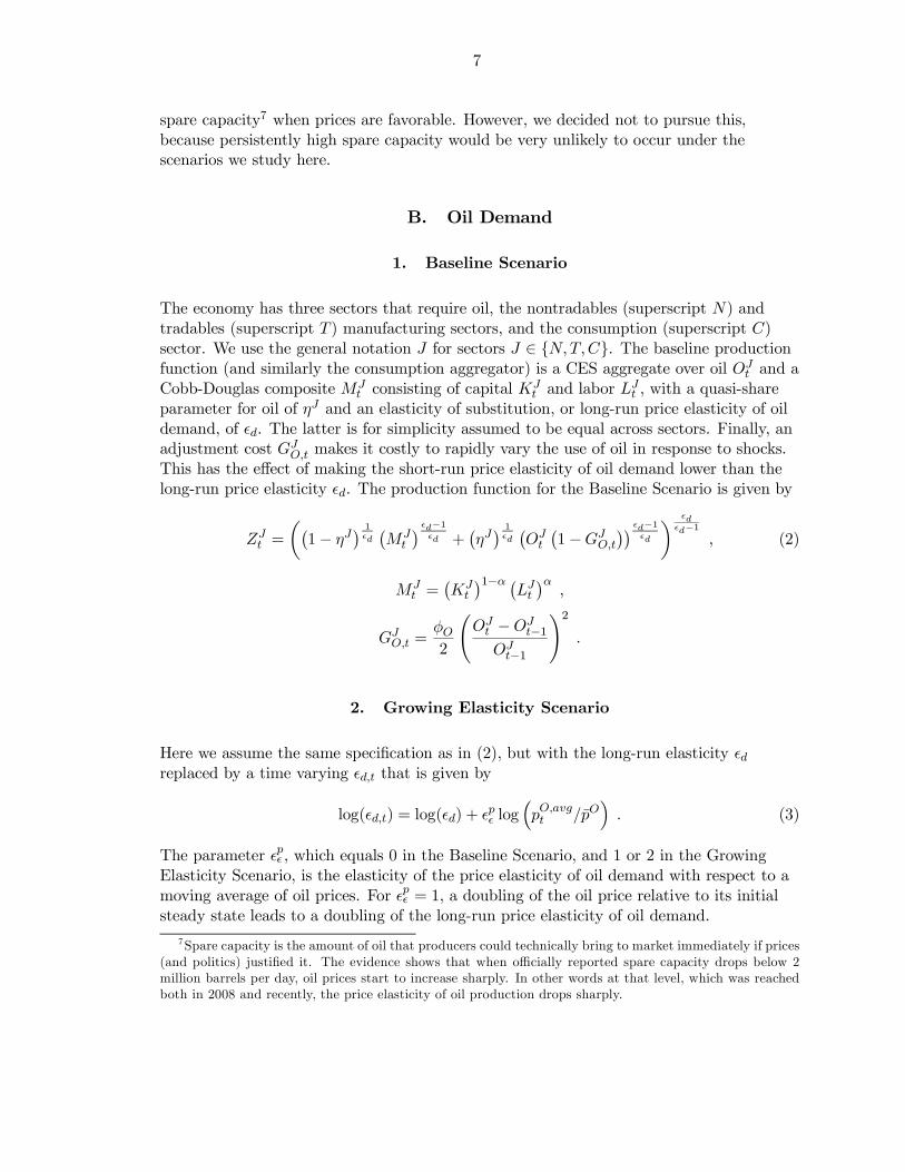
The economy has three sectors that require oil, the nontradables (superscript N) andtradables (superscript T ) manufacturing sectors, and the consumption (superscript C)sector. We use the general notation J for sectors J ∈ {N,T,C}. The baseline productionfunction (and similarly the consumption aggregator) is a CES aggregate over oil OJt and aCobb-Douglas composite MJ
t consisting of capital KJt and labor LJt , with a quasi-share
parameter for oil of ηJ and an elasticity of substitution, or long-run price elasticity of oildemand, of ǫd. The latter is for simplicity assumed to be equal across sectors. Finally, anadjustment cost GJO,t makes it costly to rapidly vary the use of oil in response to shocks.This has the effect of making the short-run price elasticity of oil demand lower than thelong-run price elasticity ǫd. The production function for the Baseline Scenario is given by
ZJt =
((1− ηJ
) 1
ǫd
(MJt
) ǫd−1ǫd +
(ηJ) 1
ǫd
(OJt(1−GJO,t
)) ǫd−1ǫd
) ǫd
ǫd−1
, (2)
MJt =
(KJt
)1−α (LJt)α,
GJO,t =φO2
(OJt −O
Jt−1
OJt−1
)2.
2. Growing Elasticity Scenario
Here we assume the same specification as in (2), but with the long-run elasticity ǫdreplaced by a time varying ǫd,t that is given by
log(ǫd,t) = log(ǫd) + ǫpǫ log
(pO,avgt /pO
). (3)
The parameter ǫpǫ , which equals 0 in the Baseline Scenario, and 1 or 2 in the GrowingElasticity Scenario, is the elasticity of the price elasticity of oil demand with respect to amoving average of oil prices. For ǫpǫ = 1, a doubling of the oil price relative to its initialsteady state leads to a doubling of the long-run price elasticity of oil demand.
7Spare capacity is the amount of oil that producers could technically bring to market immediately if prices(and politics) justified it. The evidence shows that when officially reported spare capacity drops below 2million barrels per day, oil prices start to increase sharply. In other words at that level, which was reachedboth in 2008 and recently, the price elasticity of oil production drops sharply.
8
3. Entropy Boundary and Falling Elasticity Scenarios
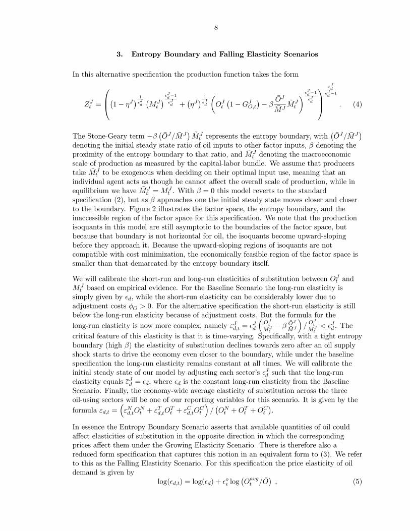
In this alternative specification the production function takes the form
ZJt =
(1− ηJ
) 1
ǫJ
d
(MJt
) ǫJd−1
ǫJ
d +(ηJ) 1
ǫJ
d
(OJt(1−GJO,t
)− β
OJ
MJMJt
) ǫJd−1
ǫJd
ǫJd
ǫJd−1
. (4)
The Stone-Geary term −β(OJ/MJ
)MJt represents the entropy boundary, with
(OJ/MJ
)
denoting the initial steady state ratio of oil inputs to other factor inputs, β denoting theproximity of the entropy boundary to that ratio, and MJ
t denoting the macroeconomicscale of production as measured by the capital-labor bundle. We assume that producerstake MJ
t to be exogenous when deciding on their optimal input use, meaning that anindividual agent acts as though he cannot affect the overall scale of production, while inequilibrium we have MJ
t =MJt . With β = 0 this model reverts to the standard
specification (2), but as β approaches one the initial steady state moves closer and closerto the boundary. Figure 2 illustrates the factor space, the entropy boundary, and theinaccessible region of the factor space for this specification. We note that the productionisoquants in this model are still asymptotic to the boundaries of the factor space, butbecause that boundary is not horizontal for oil, the isoquants become upward-slopingbefore they approach it. Because the upward-sloping regions of isoquants are notcompatible with cost minimization, the economically feasible region of the factor space issmaller than that demarcated by the entropy boundary itself.
We will calibrate the short-run and long-run elasticities of substitution between OJt andMJt based on empirical evidence. For the Baseline Scenario the long-run elasticity is
simply given by ǫd, while the short-run elasticity can be considerably lower due toadjustment costs φO > 0. For the alternative specification the short-run elasticity is stillbelow the long-run elasticity because of adjustment costs. But the formula for the
long-run elasticity is now more complex, namely εJd,t = ǫJd
(OJt
MJt
− β OJ
MJ
)/OJt
MJt
< ǫJd . The
critical feature of this elasticity is that it is time-varying. Specifically, with a tight entropyboundary (high β) the elasticity of substitution declines towards zero after an oil supplyshock starts to drive the economy even closer to the boundary, while under the baselinespecification the long-run elasticity remains constant at all times. We will calibrate theinitial steady state of our model by adjusting each sector’s ǫJd such that the long-runelasticity equals εJd = ǫd, where ǫd is the constant long-run elasticity from the BaselineScenario. Finally, the economy-wide average elasticity of substitution across the threeoil-using sectors will be one of our reporting variables for this scenario. It is given by the
formula εd,t =(εNd,tO
Nt + ε
Td,tO
Tt + ε
Cd,tO
Ct
)/(ONt +O
Tt +O
Ct
).
In essence the Entropy Boundary Scenario asserts that available quantities of oil couldaffect elasticities of substitution in the opposite direction in which the correspondingprices affect them under the Growing Elasticity Scenario. There is therefore also areduced form specification that captures this notion in an equivalent form to (3). We referto this as the Falling Elasticity Scenario. For this specification the price elasticity of oildemand is given by
log(ǫd,t) = log(ǫd) + ǫoǫ log
(Oavgt /O
), (5)

9
where Oavgt =(Ot(Oavgt−1
)3) 1
4
. We will present the results for this scenario alongside the
Entropy Boundary Scenario. The reason for presenting both, as we will explain, is partlythat we have encountered computational limits when solving the model under the EntropyBoundary Scenario.
4. Technology Externality Scenario
In this specification the production function takes the form
ZJt =
(1− ηJ
) 1
ǫJ
d
(MJt
) ǫJd−1
ǫJ
d +(ηJ) 1
ǫJ
d
(OJtOJ
)ξJ
OJt(1−GJO,t
)
ǫJd−1
ǫJd
ǫJd
ǫJ
d−1
. (6)
The term(OJt /O
J)ξJ
represents oil-augmenting technology, with OJ denoting steady
state oil use, and OJt representing actual oil use. Agents treat OJt as external whenequating the value of the marginal product of oil to the price of oil, while in equilibriumwe have OJt = O
Jt . This specification implies that the cost share of oil remains below its
output contribution when ξJ > 0. The beneficial effects of oil are therefore not capturedexclusively by the suppliers of oil, but rather by all factors of production, in the same wayas for any other factor-augmenting technological change.
C. World Oil Market Equilibrium
Letting i index the six regions of the world economy, the market clearing condition for theworld oil market is given by
Σ6i=1Osupt (i) = Σ6i=1
(ONt (i) +O
Tt (i) +O
Ct (i)
), (7)
where the world oil price adjusts to equilibrate oil supply and oil demand.
D. Calibration
The long-term price elasticity of oil demand in both production and consumption isassumed to equal 0.08, while the short-term elasticity, which reflects the interaction of thelong-term elasticity and the size of adjustment costs, is around 0.02. This is consistentwith estimates for 1990—2009 contained in Helbling and others (2011), and also with theBayesian estimation results in Benes and others (2012).
In the baseline the contribution of oil to output is determined by the oil cost share. Basedon a careful evaluation of recent historical data for the six regions of the model economy,this cost share has been calibrated at 2 to 5 percent, depending on the sector and region.

10
The model assumes balanced growth, which means that the long-run income elasticity ofoil demand is equal to one. This appears to be inconsistent with the data, as Helbling andothers (2011) estimate a long-run income elasticity of only around one third at the worldlevel (the short-term income elasticity is much higher, at 0.68), based on data from theperiod after 1990. This aspect will play a prominent role in our discussion of the results.
The literature contains far fewer studies that estimate the price elasticity of oil supply.But Benes and others (2012), who use a nonlinear Bayesian specification, are able toseparately identify demand and supply elasticities. They find short-run price elasticities ofsupply, which represent the ability of oil producers to utilize existing spare capacity, ofbetween 0.05 and 0.15. They also separately estimate long-run price elasticities, whichcorrespond almost exactly to the coefficient ǫs in our specification, and find them to bemuch lower at between 0.005 and 0.02. Our specification omits short-run price elasticities,based on the reasonable assumption that the decline in the growth rate of world oil outputin all our scenarios will eliminate spare capacity going forward. At the same time, ourcalibration of the long-run price elasticity of oil supply, at ǫs = 0.03, is slightly higher thanthe estimate of Benes and others (2012).
Because we model oil supply as an endowment, we need to specify how the revenue fromoil sales is divided into extraction costs and payments to owners. We assume that, prior tothe decline in the growth rate of oil supply, 40 percent of oil revenue must be used to payfor intermediate goods inputs, and that thereafter the real extraction cost per barrel of oilincreases at a constant annual rate of 2 percent. The remainder of oil revenue is the oilrent, which is distributed between the private sector and the government. In the netoil-importing regions of our model economy, the government is assumed to receive only avery small portion of the oil rent. However, in oil exporters it is assumed to receive 90percent, reflecting the fact that in many of these countries the oil sector is dominated bystate-owned oil companies. Critically, we assume that governments do not immediatelyspend the additional funds, but that they accumulate them in a U.S. dollar—based fundthat is spent gradually over time, at a rate of 3 percent per annum. One of the key effectsof an increase in the oil price is therefore a dramatic increase in world savings due to thelow propensity to consume out of oil revenues of oil exporters’ governments.
III. Discussion of the Alternative Specifications
A. Entropy Boundary and Falling Elasticity Scenarios
Economists generally assume that elasticities of substitution between oil and other factorsof production must be higher in the long run than in the short run. There are two possiblereasons for this view. First, as in our Baseline Scenario, adjustment costs drive theshort-run elasticity below the constant long-run elasticity ǫd. Second, as in our GrowingElasticity Scenario, for persistently very high oil prices, ǫd may no longer be constant, butmay instead grow with oil prices. On the other hand, several contributions in the naturalsciences have objected that the assumption of a constant or growing long-run elasticity isnot consistent with the historical facts (Smil (2010)), with real-world practical limits tosubstitution (Ayres (2007)), or with the laws of thermodynamics, specifically with entropy

11
(Reynolds (2002)). In this paper we mathematically formalize Reynolds’ entropyboundary as a Stone-Geary production function whereby the use of oil has to exceed acertain minimum multiple of the use of other factors of production. This implies that afteran oil supply shock elasticities are very low in the short run (due to adjustment costs),significantly higher in the medium run (as adjustment costs are overcome), but potentiallymuch lower again in the long run if the shock is sufficiently large, because there is a finitelimit to the extent that machines (and labor) can substitute for oil. The Falling ElasticityScenario attempts to capture the same logic in a reduced form.
The argument for an entropy boundary in the oil-capital/labor factor space requires a setof two interrelated arguments that draw on physics and engineering.
Entropy relates to energy rather than specifically to oil. It therefore affects theenergy-capital/labor factor space. Entropy, or the Second Law of Thermodynamics, statesthat any ordered system naturally tends towards disorder through energy dissipation.Maintaining the system therefore requires the constant addition of a flow of energy.Applied to capital put in place to substitute away from energy, this means that suchcapital needs a continuing minimum input of energy to remain useful. A continuing inputof capital, to offset depreciation, is not enough. Critically, this implies that only energy inexcess of that minimum necessary amount can start to add to the output of goods. Thisputs a boundary on the factor space that can be accessed, with near-zero energy input notan option. When factor use comes close to that boundary, the elasticity of substitutionbetween energy and other factors must go to zero.
To relate this concept to the oil-capital/labor factor space, we need to consider therelationship between oil and energy. If oil and other forms of energy had to be used inproportions that cannot change sufficiently, or sufficiently rapidly, an entropy boundaryfor energy implies an entropy boundary for oil. The two critical questions are thereforewhether other energy sources can technically substitute for oil over realistic time horizons(years rather than decades) and at the required scale, and whether such energy sourceshave their own supply limitations. The argument that substitution away from oil would beextremely costly and time-consuming was first made by the Hirsch and others (2005)report for the U.S. Department of Energy, a government-supported analysis of the shortesttime required to mitigate a decline in world oil production. This study claimed that theU.S. economy would require a lead time of at least 20 years to prepare alternatives to anoil-based economy, with any shorter preparation time implying serious transitionproblems. The 20-year estimate takes known saving and substitution possibilities intoaccount. For the automotive sector this includes the possibility of using natural gas andelectricity as alternatives to oil-based fuels, especially in densely populated areas.
We next discuss some of the energy alternatives to oil in more detail, both concerningtheir potential supply limitations, and concerning their technical substitutability for oil inspecific applications.
1. Supply Limitations
We begin with the least plausible substitute for oil, renewables, and then move on toprogressively closer substitutes.
12
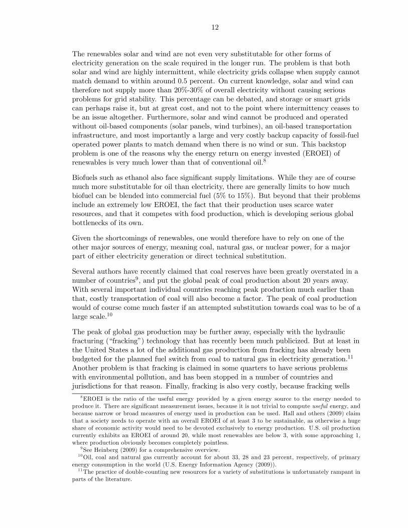
The renewables solar and wind are not even very substitutable for other forms ofelectricity generation on the scale required in the longer run. The problem is that bothsolar and wind are highly intermittent, while electricity grids collapse when supply cannotmatch demand to within around 0.5 percent. On current knowledge, solar and wind cantherefore not supply more than 20%-30% of overall electricity without causing seriousproblems for grid stability. This percentage can be debated, and storage or smart gridscan perhaps raise it, but at great cost, and not to the point where intermittency ceases tobe an issue altogether. Furthermore, solar and wind cannot be produced and operatedwithout oil-based components (solar panels, wind turbines), an oil-based transportationinfrastructure, and most importantly a large and very costly backup capacity of fossil-fueloperated power plants to match demand when there is no wind or sun. This backstopproblem is one of the reasons why the energy return on energy invested (EROEI) ofrenewables is very much lower than that of conventional oil.8
Biofuels such as ethanol also face significant supply limitations. While they are of coursemuch more substitutable for oil than electricity, there are generally limits to how muchbiofuel can be blended into commercial fuel (5% to 15%). But beyond that their problemsinclude an extremely low EROEI, the fact that their production uses scarce waterresources, and that it competes with food production, which is developing serious globalbottlenecks of its own.
Given the shortcomings of renewables, one would therefore have to rely on one of theother major sources of energy, meaning coal, natural gas, or nuclear power, for a majorpart of either electricity generation or direct technical substitution.
Several authors have recently claimed that coal reserves have been greatly overstated in anumber of countries9, and put the global peak of coal production about 20 years away.With several important individual countries reaching peak production much earlier thanthat, costly transportation of coal will also become a factor. The peak of coal productionwould of course come much faster if an attempted substitution towards coal was to be of alarge scale.10
The peak of global gas production may be further away, especially with the hydraulicfracturing (“fracking”) technology that has recently been much publicized. But at least inthe United States a lot of the additional gas production from fracking has already beenbudgeted for the planned fuel switch from coal to natural gas in electricity generation.11
Another problem is that fracking is claimed in some quarters to have serious problemswith environmental pollution, and has been stopped in a number of countries andjurisdictions for that reason. Finally, fracking is also very costly, because fracking wells
8EROEI is the ratio of the useful energy provided by a given energy source to the energy needed toproduce it. There are significant measurement issues, because it is not trivial to compute useful energy, andbecause narrow or broad measures of energy used in production can be used. Hall and others (2009) claimthat a society needs to operate with an overall EROEI of at least 3 to be sustainable, as otherwise a hugeshare of economic activity would need to be devoted exclusively to energy production. U.S. oil productioncurrently exhibits an EROEI of around 20, while most renewables are below 3, with some approaching 1,where production obviously becomes completely pointless.
9See Heinberg (2009) for a comprehensive overview.10Oil, coal and natural gas currently account for about 33, 28 and 23 percent, respectively, of primary
energy consumption in the world (U.S. Energy Information Agency (2009)).11The practice of double-counting new resources for a variety of substitutions is unfortunately rampant in
parts of the literature.

13
and fields exhibit extremely fast decline rates and therefore require constant new drillingto maintain production. Berman (2012) contains an excellent overview of the problemswith natural gas for the U.S. case. They include an extreme acceleration of sector-wideaverage decline rates of gas wells, and therefore of extraction costs, and a largeoverstatement of field reserves for financial reporting reasons. If Berman’s prognoses turnout to be correct, natural gas prices could soon begin a rapid rise that would significantlyreduce its cost advantage over oil, and therefore the incentive to switch from oil to gas.The expectation that that cost advantage is not just large today but also highly persistentis critical, because a switch to electricity produced by natural gas would require thebuilding of costly power plants, which have amortization periods of 30 years or more(Bishop and others (2012)), while a direct switch to natural gas as a transportation fuel,which is technically among the most realistic substitution possibilities, would require theinstallation of a costly network of filling stations.12
As for nuclear power, Dittmar (2011) recently estimated that if large-scale substitutionfrom fossil fuels towards nuclear power was attempted, the benefits would be veryshort-lived because the world would hit a peak in uranium production in short order. Butthis finding is highly controversial, with others claiming that different reactor types wouldeliminate problems with fuel supply for the foreseeable future. In any event, theworldwide trend seems to be going away from rather than towards nuclear power, due tothe fear of low-probability but extremely high-cost events such as Fukushima.
To summarize, other non-renewable energy sources may also have supply limits, and thereis at least a possibility that they may not be able to provide energy security over the longrun.
2. Technical Substitutability
In addition to supply limits there are also limits to the technical substitutability of coal,gas or electricity for oil. We start with the observation that the main uses of oil in today’seconomy are as a liquid transportation fuel and as a feedstock for the chemical industry.Critical considerations for technical substitutability include, relative to any specificapplication, storability, transportability, and most importantly the ability to deliver usefulenergy. An example is the impossibility of running an airplane with coal, which is due tocoal’s physical properties rather than simply its energy content.
The most important use of oil today is in transportation. The properties of oil, or moregenerally liquid fuels, in this application are far superior to the alternatives. In some casesa transition towards a transportation infrastructure based on electricity, natural gasand/or liquid fuels derived from non-oil sources may be possible by retrofitting existingequipment or building differently configured new equipment. But a large-scale transitionwould be enormously expensive in terms of dollars13, in terms of energy, and mostimportantly in terms of time - the transition would require several decades. This,according to the best available scientific evidence (Hirsch and others (2005), UK EnergyResearch Centre (2009)), is time that we may not have.
12Gas filling stations require significantly greater safety precautions than conventional filling stations.13This is why coal-to-liquids or gas-to-liquids industries have not yet been established on a significant
scale, except in countries that have faced economic sanctions or economic isolation.

14
The second main use of oil today is as a feedstock of the chemical industry. Oil productsare in virtually every single product we consume, either directly, or in the mining of therespective raw materials, in transportation or in processing. In most cases there simply isno easy substitute for oil derivatives in these applications, although in some specific casesthere are possibilities to derive the chemicals from coal or gas instead.
B. Growing Elasticity Scenario
For the next several years substitution away from oil and towards gas or electricity may besufficient to delay the moment at which lower oil availability could cause serious economicproblems. Given the proven technical feasibility of some substitution technologies, such asgas-powered vehicles, and to a lesser extent coal-to-liquids and gas-to-liquids, it maytherefore be reasonable to assume that price elasticities of demand have scope to rise for anumber of years. This is true even if one were to subscribe to the view that thealternatives have significant supply limitations in the not too distant future, that they canonly technically substitute for oil in a limited number of applications, and that attemptsto economize on oil use may soon run into limits dictated by entropy. It is for this reasonthat we include the Growing Elasticity Scenario in this study. It is impossible to know atthe present time which effect on price elasticities of oil demand will be stronger and forhow long.
C. Technology Externality Scenario
For the contribution of oil to GDP, the main problem is that conventional productionfunctions imply an equality of cost shares and output contributions of oil. This has ledeconomists to conclude that, given its historically low cost share of around 3.5% for theU.S. economy14, oil can never account for a massive output contraction, even with lowelasticities of substitution between oil and other factors of production. There are twocounterarguments to this. First, if oil prices were to permanently rise sharply due tosupply shocks, then cost shares would become high enough to worry even if outputcontributions equalled cost shares. Second, several recent articles and books by naturalscientists have argued that output contributions of energy/oil need not equal cost shareswith a more appropriate modeling of the aggregate technology. The contributions includeAyres and Warr (2005, 2010), Hall and Klitgaard (2011), Kümmel (2011), and Kümmeland others (2002), who propose alternative production functions that are based onconcepts from engineering and thermodynamics. In our alternative specification oil entersexternally in a similar fashion to technology. This feature can yield output contributionsof oil that are higher than cost shares as long as ξJ > 0.
14See http://www.eia.gov/oiaf/economy/energy_price.html.

15
IV. Simulation Results
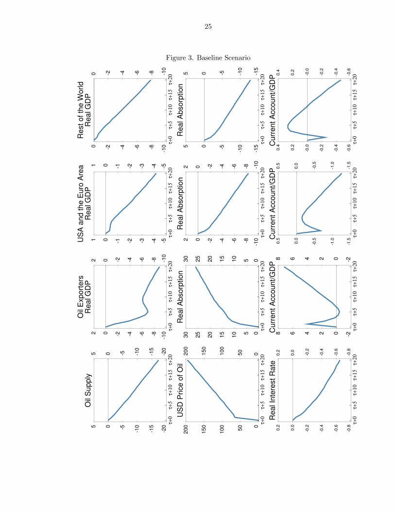
Figures 3-8 present the results of our simulations. Variables are shown, where applicable,relative to trend. The first column shows the evolution of the world oil supply, the real oilprice (in terms of U.S. goods), and the world average real interest rate. The second columnshows real GDP, real absorption, and the current account-to-GDP ratio for oil exporters.15
The third and fourth columns show the same three variables for the United States plusEuro Area region, and for the Rest of the World group of countries. Aggregations acrossregions of the world economy use purchasing power parity (PPP) weights to fix relativecountry sizes. As shown in Helbling and others (2011), there are some interesting furtherdifferences in the reactions of individual regions to higher oil prices, but the commonfeatures across regions are far more interesting, and we have therefore decided to focus onthem in this paper. The year in which the oil supply shock hits the economy is denoted byτ , and as mentioned above a range of different values for τ are justifiable.
A. Baseline Scenario
The Baseline Scenario analyzes the impact of a decline in the average growth rate of worldoil production by 1 percentage point below its historical trend growth rate starting in yearτ , with an eventual return to the initial growth rate in year τ + 30.16 As in all simulationsthat follow, agents are assumed to be surprised by the shock, but thereafter they perfectlyforesee the future evolution of world oil production.
The shock generates an immediate oil price spike of over 60 percent. This reflects the verylow short-term price elasticity of oil demand. Because the decline in supply is persistent,the real oil price continues to increase thereafter, as market equilibrium requires ongoingdemand destruction. Over 10- and 20-year horizons, the cumulative oil price increasesamount to just over 100 percent and 200 percent. The 10-year result is extremely close tothe point forecast in Benes and others (2012).
The reduced availability of oil, and the resulting higher oil prices, lead to a reduction inGDP levels, and to larger current account deficits, in oil importers. In the short term theglobal adjustment is also shaped by the wealth transfer from oil importers to oil exporters,which has effects on trade and capital flows.
With rising oil prices, oil exporters experience sustained increases in income and wealth.As a result, their domestic demand (domestic absorption) increases ahead of GDP, at aninitial rate of over 2 percent annually. Higher spending leads to upward domestic pricepressures and a large real appreciation. This “Dutch disease” effect reduces output in thetradables sector (other than oil), thereby reducing GDP by up to 7 percent below trendover the first five years, and by almost 10 percent after 20 years. The current accountimprovement in this group of countries, which equals up to 4 percent of GDP in the veryshort run and almost 8 percent after 20 years, is due entirely to the higher value of oil
15Oil exporters include the following countries: Algeria, Angola, Azerbaijan, Bahrain, Canada, Republicof Congo, Equatorial Guinea, Iraq, Kuwait, Libya, Mexico, Nigeria, Norway, Oman, Qatar, Russia, SaudiArabia, United Arab Emirates and Venezuela.
16For technical reasons it is not possible to simulate a completely permanent shock to this growth rate.
16
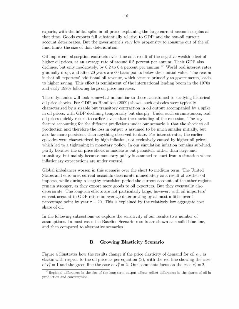
exports, with the initial spike in oil prices explaining the large current account surplus atthat time. Goods exports fall substantially relative to GDP, and the non-oil currentaccount deteriorates. But the government’s very low propensity to consume out of the oilfund limits the size of that deterioration.
Oil importers’ absorption contracts over time as a result of the negative wealth effect ofhigher oil prices, at an average rate of around 0.5 percent per annum. Their GDP alsodeclines, but only moderately, by 0.2 to 0.4 percent per annum.17 World real interest ratesgradually drop, and after 20 years are 60 basis points below their initial value. The reasonis that oil exporters’ additional oil revenue, which accrues primarily to governments, leadsto higher saving. This effect is reminiscent of the international lending boom in the 1970sand early 1980s following large oil price increases.
These dynamics will look somewhat unfamiliar to those accustomed to studying historicaloil price shocks. For GDP, as Hamilton (2009) shows, such episodes were typicallycharacterized by a sizable but transitory contraction in oil output accompanied by a spikein oil prices, with GDP declining temporarily but sharply. Under such circumstances, realoil prices quickly return to earlier levels after the unwinding of the recession. The keyfeature accounting for the different predictions under our scenario is that the shock to oilproduction and therefore the loss in output is assumed to be much smaller initially, butalso far more persistent than anything observed to date. For interest rates, the earlierepisodes were characterized by high inflation, not exclusively caused by higher oil prices,which led to a tightening in monetary policy. In our simulation inflation remains subdued,partly because the oil price shock is moderate but persistent rather than large andtransitory, but mainly because monetary policy is assumed to start from a situation whereinflationary expectations are under control.
Global imbalances worsen in this scenario over the short to medium term. The UnitedStates and euro area current accounts deteriorate immediately as a result of costlier oilimports, while during a lengthy transition period the current accounts of the other regionsremain stronger, as they export more goods to oil exporters. But they eventually alsodeteriorate. The long-run effects are not particularly large, however, with oil importers’current account-to-GDP ratios on average deteriorating by at most a little over 1percentage point by year τ + 20. This is explained by the relatively low aggregate costshare of oil.
In the following subsections we explore the sensitivity of our results to a number ofassumptions. In most cases the Baseline Scenario results are shown as a solid blue line,and then compared to alternative scenarios.
B. Growing Elasticity Scenario
Figure 4 illustrates how the results change if the price elasticity of demand for oil ǫd,t iselastic with respect to the oil price as per equation (3), with the red line showing the caseof ǫpǫ = 1 and the green line the case of ǫpǫ = 2. Our comments focus on the case ǫpǫ = 2,
17Regional differences in the size of the long-term output effects reflect differences in the shares of oil inproduction and consumption.

17
where we observe that the oil price only needs to rise by half as much as in the BaselineScenario to bring about the necessary substitution. The effects on GDP are positiveeverywhere, with roughly 50 percent smaller contractions in oil exporters, the UnitedStates and the euro area, and an even larger turnaround in the Rest of the Worldcountries, where an 8 percent output loss over 20 years turns into a 2 to 3 percent outputgain.
The latter is driven mainly by emerging Asia and to a lesser extent Japan. Under theBaseline Scenario these two regions, whose production is heavily manufacturing-based andtherefore oil-intensive, suffer very large contractionary effects of lower oil availability andhigher oil prices. Under the Growing Elasticity Scenario, where oil is less critical becauseof its higher substitutability, these contractionary effects are much smaller, and twocountervailing effects are now strong enough to raise rather than contract output. Thefirst of these is a surge in goods exports to oil importers to satisfy their increasingdomestic demand. Emerging Asia and Japan have particularly strong export linkages tooil exporters and therefore benefit disproportionately. The second countervailing effect is asurge in investment demand in response to lower world real interest rates, which isparticularly strong in emerging Asia because of its higher steady state investment-to-GDPratio.
As for global current account imbalances, these are less severe under this scenario, withsmaller surpluses for oil exporters and emerging Asia, and smaller deficits for the larger oilimporters.
C. Entropy Boundary Scenario and Falling Elasticity Scenario
Figure 5 illustrates four simulations of our Baseline Scenario shock, with the technologynow given by (4), and for the cases of β ∈ {0, 0.3, 0.6, 0.9}. The case of β = 0 is identicalto the Baseline Scenario. For larger β the entropy boundary is tighter, in other wordscloser to initial steady state factor allocation, which means that further substitution awayfrom oil becomes harder at a faster rate. The bottom left panel of Figure 5 shows theaverage elasticity of substitution εd,t.
We observe that for a tighter entropy boundary the increase in the oil price is significantlylarger. The reason is that the elasticity of substitution moves closer to zero as the supplyconstraint starts to get progressively worse. For the tightest boundary (β = 0.9) the oilprice increases by almost 300 percent rather than by 200 percent after 20 years.
Oil exporters experience a larger positive wealth effect if β is larger. The resulting largerabsorption, real exchange rate appreciation and “Dutch disease” effect cause a largerinitial output contraction in that region, but eventually output in that region alsoexperiences a larger rebound, because over time governments start to spend more andmore of the accumulated oil surpluses, which are now larger due to higher oil prices. Oilimporters experience worse contractions in absorption and output when the economystarts closer to the entropy boundary, and current account imbalances get larger, but thesize of these effects is fairly small.
The reason is partly computational. For all simulations reported in this paper except for
18
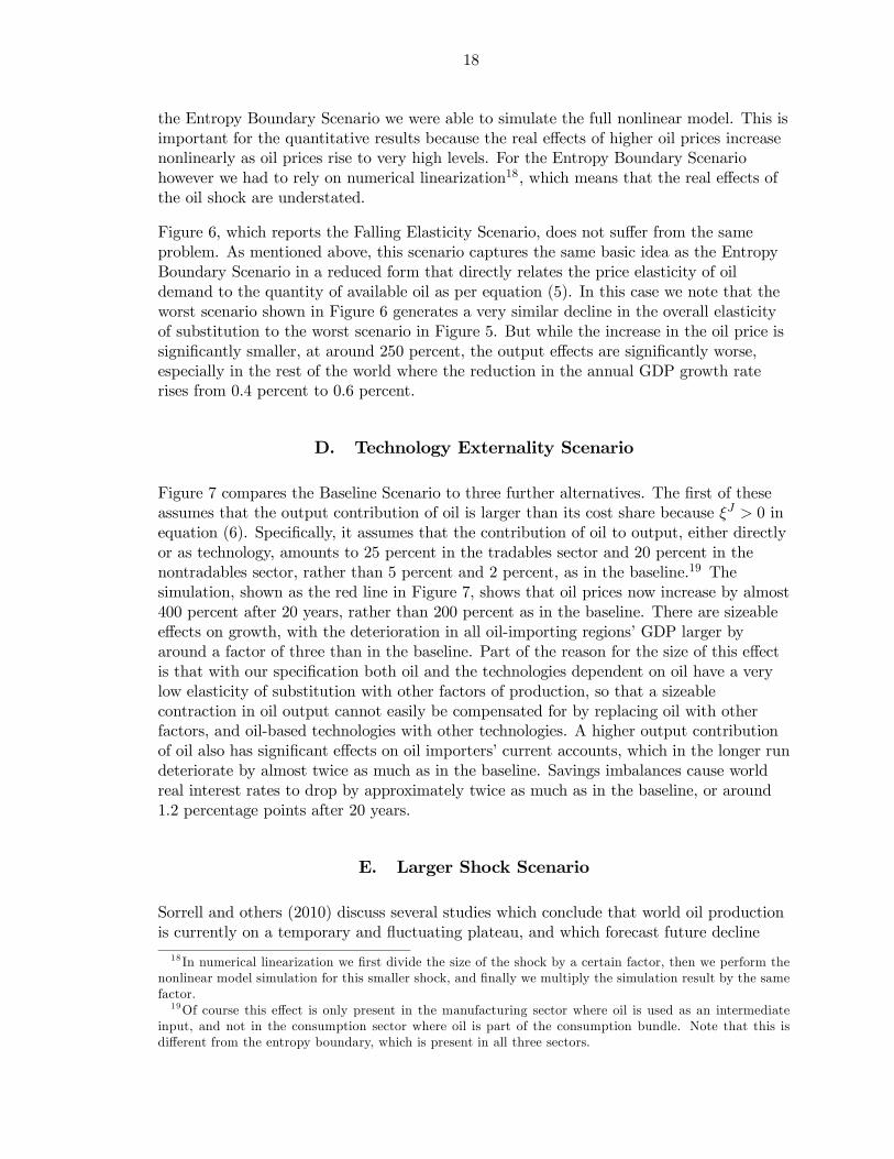
the Entropy Boundary Scenario we were able to simulate the full nonlinear model. This isimportant for the quantitative results because the real effects of higher oil prices increasenonlinearly as oil prices rise to very high levels. For the Entropy Boundary Scenariohowever we had to rely on numerical linearization18, which means that the real effects ofthe oil shock are understated.
Figure 6, which reports the Falling Elasticity Scenario, does not suffer from the sameproblem. As mentioned above, this scenario captures the same basic idea as the EntropyBoundary Scenario in a reduced form that directly relates the price elasticity of oildemand to the quantity of available oil as per equation (5). In this case we note that theworst scenario shown in Figure 6 generates a very similar decline in the overall elasticityof substitution to the worst scenario in Figure 5. But while the increase in the oil price issignificantly smaller, at around 250 percent, the output effects are significantly worse,especially in the rest of the world where the reduction in the annual GDP growth raterises from 0.4 percent to 0.6 percent.
D. Technology Externality Scenario
Figure 7 compares the Baseline Scenario to three further alternatives. The first of theseassumes that the output contribution of oil is larger than its cost share because ξJ > 0 inequation (6). Specifically, it assumes that the contribution of oil to output, either directlyor as technology, amounts to 25 percent in the tradables sector and 20 percent in thenontradables sector, rather than 5 percent and 2 percent, as in the baseline.19 Thesimulation, shown as the red line in Figure 7, shows that oil prices now increase by almost400 percent after 20 years, rather than 200 percent as in the baseline. There are sizeableeffects on growth, with the deterioration in all oil-importing regions’ GDP larger byaround a factor of three than in the baseline. Part of the reason for the size of this effectis that with our specification both oil and the technologies dependent on oil have a verylow elasticity of substitution with other factors of production, so that a sizeablecontraction in oil output cannot easily be compensated for by replacing oil with otherfactors, and oil-based technologies with other technologies. A higher output contributionof oil also has significant effects on oil importers’ current accounts, which in the longer rundeteriorate by almost twice as much as in the baseline. Savings imbalances cause worldreal interest rates to drop by approximately twice as much as in the baseline, or around1.2 percentage points after 20 years.
E. Larger Shock Scenario
Sorrell and others (2010) discuss several studies which conclude that world oil productionis currently on a temporary and fluctuating plateau, and which forecast future decline
18 In numerical linearization we first divide the size of the shock by a certain factor, then we perform thenonlinear model simulation for this smaller shock, and finally we multiply the simulation result by the samefactor.
19Of course this effect is only present in the manufacturing sector where oil is used as an intermediateinput, and not in the consumption sector where oil is part of the consumption bundle. Note that this isdifferent from the entropy boundary, which is present in all three sectors.
19
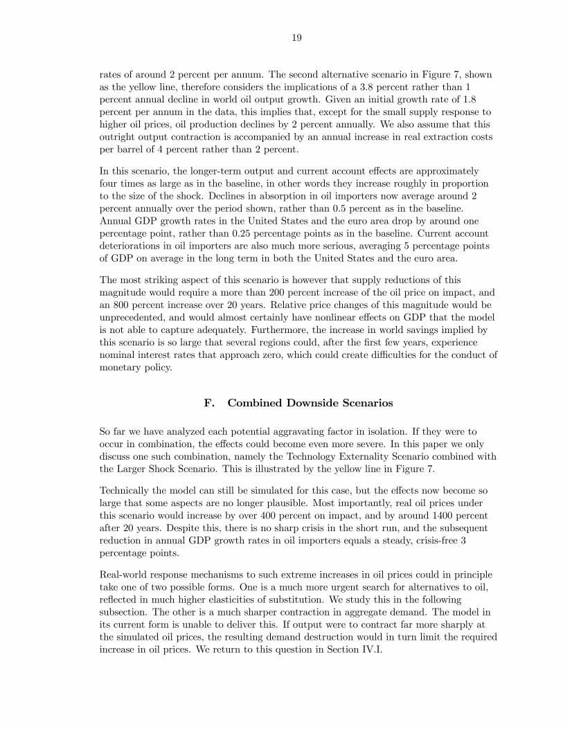
rates of around 2 percent per annum. The second alternative scenario in Figure 7, shownas the yellow line, therefore considers the implications of a 3.8 percent rather than 1percent annual decline in world oil output growth. Given an initial growth rate of 1.8percent per annum in the data, this implies that, except for the small supply response tohigher oil prices, oil production declines by 2 percent annually. We also assume that thisoutright output contraction is accompanied by an annual increase in real extraction costsper barrel of 4 percent rather than 2 percent.
In this scenario, the longer-term output and current account effects are approximatelyfour times as large as in the baseline, in other words they increase roughly in proportionto the size of the shock. Declines in absorption in oil importers now average around 2percent annually over the period shown, rather than 0.5 percent as in the baseline.Annual GDP growth rates in the United States and the euro area drop by around onepercentage point, rather than 0.25 percentage points as in the baseline. Current accountdeteriorations in oil importers are also much more serious, averaging 5 percentage pointsof GDP on average in the long term in both the United States and the euro area.
The most striking aspect of this scenario is however that supply reductions of thismagnitude would require a more than 200 percent increase of the oil price on impact, andan 800 percent increase over 20 years. Relative price changes of this magnitude would beunprecedented, and would almost certainly have nonlinear effects on GDP that the modelis not able to capture adequately. Furthermore, the increase in world savings implied bythis scenario is so large that several regions could, after the first few years, experiencenominal interest rates that approach zero, which could create difficulties for the conduct ofmonetary policy.
F. Combined Downside Scenarios
So far we have analyzed each potential aggravating factor in isolation. If they were tooccur in combination, the effects could become even more severe. In this paper we onlydiscuss one such combination, namely the Technology Externality Scenario combined withthe Larger Shock Scenario. This is illustrated by the yellow line in Figure 7.
Technically the model can still be simulated for this case, but the effects now become solarge that some aspects are no longer plausible. Most importantly, real oil prices underthis scenario would increase by over 400 percent on impact, and by around 1400 percentafter 20 years. Despite this, there is no sharp crisis in the short run, and the subsequentreduction in annual GDP growth rates in oil importers equals a steady, crisis-free 3percentage points.
Real-world response mechanisms to such extreme increases in oil prices could in principletake one of two possible forms. One is a much more urgent search for alternatives to oil,reflected in much higher elasticities of substitution. We study this in the followingsubsection. The other is a much sharper contraction in aggregate demand. The model inits current form is unable to deliver this. If output were to contract far more sharply atthe simulated oil prices, the resulting demand destruction would in turn limit the requiredincrease in oil prices. We return to this question in Section IV.I.
20
G. Combined Downside and Growing Elasticity Scenario
In Figure 8 we combine the worst case of Figure 7 with the Growing Elasticity Scenario.For the case of ǫpǫ = 2 we observe that the increase in the oil price is only half as large, andso are, approximately, the output effects. But this still leaves an oil price increase of 800percent after 20 years. More broadly, unless the increase in the price elasticity of demandin response to higher oil price is extreme, and we have discussed above why this is notlikely, then the worst of our downside scenarios would still force the economy to cope withentirely unprecedented increases in oil prices. In the real world, if such a scenario came topass, the more likely outcome would therefore include not only higher elasticities ofsubstitution but also a larger output contraction.
H. The Assumption of Unitary Income Elasticity
As discussed in Section II.D, our model assumes a unitary income elasticity of oil demand,while the data suggest a much lower income elasticity of around one third. This empiricalregularity probably reflects the fact that much recent growth worldwide has been due tothe services sector, which uses less oil per unit of output. While a low income elasticitymay appear like a blessing in an environment where oil output can grow withoutconstraints, it actually makes the problem of supply constraints all the more severe. Thereasoning is simple-minded, but nevertheless approximately true because very low priceelasticities limit the extent of substitution away from oil. Namely, if it really only takes aone third of one percentage point increase in oil supply per annum to support additionalGDP growth of one percentage point, then it must also be true that it would only take aone third of one percentage point decrease in oil supply growth to reduce GDP growth bya full percentage point. And the kinds of declines in oil supply growth that are now beingdiscussed as realistic possibilities are far larger than one third of one percentage point.
I. The Assumption of Smooth Reallocation
In each of the scenarios in Sections IV.B to IV.G, the transition to a new equilibrium issmooth by assumption. Consumers in oil exporters easily absorb large surpluses in goodsexports from oil importers, financial markets efficiently absorb and intermediate a flood ofsavings from oil exporters, businesses respond flexibly to higher oil prices by reallocatingresources, and workers readily accept lower real wages. Some of these assumptions may betoo optimistic.
Historical experience suggests caution when it comes to the efficient intermediation oflarge net capital flows from oil exporters’ governments. If not efficiently allocated, riskpremia could increase in parts of the world where borrowers are vulnerable. This, in turn,could prevent borrowers from taking advantage of lower risk-free interest rates, which isan important mitigation mechanism in the face of oil scarcity. If private as well as publicsaving rates were to increase in oil-exporting countries, this problem could intensify.
A smooth reallocation of resources among inputs and across sectors as the economy adjuststo less oil is also a very strong assumption. Unlike in the model, real economies have many

21
and highly interdependent industries, and several industries, including car manufacturing,airlines, trucking, long-distance trade, and tourism, would be affected by an oil shockmuch earlier and much more seriously than others. The adverse effects of large-scalebankruptcies in such industries could spread to the rest of the economy, either throughcorporate balance sheets (intercompany credit, interdependence of industries such asconstruction and tourism) or through bank balance sheets (lack of credit after loan losses).
In recent years, labor market flexibility has helped to improve the absorption of oil shocks(Blanchard and Galí (2007)). In the case of larger and more persistent oil price increases,however, workers may resist a series of real wage cuts. This, while perhaps mitigating thedistributional consequences of the oil shock, could significantly raise the output cost of theshock during the long transition period.
Finally, the simulations do not consider the possibility that some oil exporters mightwithhold an increasing share of their stagnating or decreasing oil output for domestic use,for example through fuel subsidies, in order to support energy intensive industries (e.g.petrochemicals), and also to forestall domestic unrest. If this were to happen, the amountof oil available to oil importers could shrink much faster than world oil output (Brown andFoucher (2010)), with obvious negative consequences for growth in those regions.
V. Conclusion
The scenarios developed in this paper highlight that the extent to which persistent oilscarcity could constrain global economic growth and current account imbalances dependscritically on a small number of key factors. If, as in our baseline, the trend growth rate ofoil output declined only modestly, and if the economy was adequately represented by astandard production function in capital, labor and oil, world output would eventuallysuffer, but the effect might not be dramatic. If the substitutability between oil and otherfactors of production was increasing in the oil price, the effect would be even smaller. Butif the reductions in oil output were more in line with the more pessimistic studies in thescientific literature, the effects could be extremely large. The same could be true if, asclaimed by several authors in the scientific literature, standard production functions missimportant aspects of the economic role of oil under conditions of scarcity. We discussedthree possibilities. First, if the economy attempted to substitute away from oil, it mightencounter a lower limit of oil use dictated by entropy. Second, the contribution of oil tooutput could be much larger than its cost share, because oil is an essential preconditionfor the continued viability of many modern technologies. Third, the income elasticity ofoil demand could be equal to one third as in some empirical studies, rather than one as inour model. And if two or more of these aggravating factors were to occur in combination,the effects could range from dramatic to downright implausible.
22
References
Ayres, R. (2007), “On the Practical Limits to Substitution”, Ecological Economics, 61,115-128.
Ayres, R. and Warr, B. (2005), “Accounting for Growth: The Role of Physical Work”,Structural Change and Economic Dynamics, 16, 181-209.
Ayres, R. and Warr, B. (2010), The Economic Growth Engine - How Energy and Work
Drive Material Prosperity, Edward Elgar Publishing.
Benes, J., Chauvet, M., Kamenik, O., Kumhof, M., Laxton, D., Mursula, S. and Selody,J. (2012), “The Future of Oil: Geology versus Technology”, IMF Working PaperWP/12/109.
Berman, A. (2012), “After The Gold Rush: A Perspective on Future U.S. Natural GasSupply and Price”, Energy Bulletin, February.
Bishop, R., Baggot, R., Kelley, W. and Fargo, R. (2012), “US Shale Oil - Shale GasProduction Potential, Part 2”, Oil & Gas Journal (forthcoming).
Blanchard, O. and Galí, J. (2007), “The Macroeconomic Effects of Oil Shocks: Why Arethe 2000s So Different from the 1970s?”, NBER Working Paper No. 13368.
Brown, J. and Foucher, J. (2010), “Peak Oil versus Peak Exports”, Energy Bulletin,available athttp://www.energybulletin.net/stories/2010-10-18/peak-oil-versus-peak-exports.
Deffeyes, K. (2005), Beyond Oil: The View from Hubbert’s Peak, Hill and Wang.
Dittmar, M. (2011), “The End of Cheap Uranium”, Working Paper, Institute of ParticlePhysics, ETH, Switzerland.
Hall, C, Balogh, S. and Murphy, D. (2009), “What is the Minimum EROI that aSustainble Society Must Have?”, Energies, 2, 25-47.
Hall, C. and Klitgaard, K. (2011), Energy and the Wealth of Nations: Understanding the
Biophysical Economy, Springer Verlag (forthcoming, June 2011).
Hamilton, J. (2009), “Causes and Consequences of the Oil Shock of 2007-08”, BrookingsPapers on Economic Activity, 215-261.
Heinberg, R. (2009), Blackout - Coal, Climate and the Last Energy Crisis, New SocietyPublishers.
Helbling, T., Kang, J.S., Kumhof, M., Muir, D., Pescatori, A. and Roache, S. (2011),“Oil Scarcity, Growth, and Global Imbalances”, World Economic Outlook, April2011, Chapter 3, International Monetary Fund.
Hirsch, R., Bezdek, R. and Wendling, R. (2005), “Peaking of World Oil Production:
23
Impacts, Mitigation and Risk Management”, United States Department of Energy.
Hirsch, R., Bezdek, R. and Wendling, R. (2010), The Impending World Energy Mess,Apogee Prime.
Hubbert, M.K. (1956), “Nuclear Energy and the Fossil Fuels”, American Petroleum
Institute Drilling and Production Practice Proceedings, pp. 5-75.
Kumhof, M., Laxton, D., Muir, D. and Mursula, S. (2010), “The Global IntegratedMonetary and Fiscal Model — Theoretical Structure”, IMF Working PaperWP/10/34.
Kümmel, R. (2011), The Second Law of Economics - Energy, Entropy, and the Origins of
Wealth, Springer Verlag.
Kümmel, R., Henn, J. and Lindenberger, D. (2002), “Capital, Labor, Energy andCreativity: Modeling Innovation Diffusion”, Structural Change and Economic
Dynamics, 13, 415-433.
Reynolds, D. (2002), Scarcity and Growth Considering Oil and Energy: An Alternative
Neo-Classical View, Edwin Mellen Press.
Smil, V. (2010), Energy Transitions - History, Requirements, Prospects, Praeger.
Sorrell, S., Miller, R., Bentley, R. and Speirs, J. (2010), “Oil Futures: A Comparison ofGlobal Supply Forecasts”, Energy Policy, 38, 4990-5003.
UK Energy Research Centre (2009), “Global Oil Depletion - An Assessment of theEvidence for a Near-Term Peak in Global Oil Production”.
United States Energy Information Administration (2009), International Energy Outlook,Washington, DC.
United States Government Accountability Office (2007), “Crude Oil: Uncertainty aboutFuture Oil Supply Makes It Important to Develop a Strategy for Addressing a Peakand Decline in World Oil Production”, Report to Congressional Requesters.
United States Joint Forces Command (2010), “The Joint Operating Environment 2010”.

24
Figure 1. World Crude Oil Production (in million barrels per day)
Figure 2. The Entropy Boundary in Factor Space
25
Figure 3. Baseline Scenario
-20
-15
-10-505
-20
-15
-10
-505
τ+
0τ+
5τ+
10
τ+
15
τ+
20
Oil
Su
pp
ly
0
50
100
150
200
050
100
150
200
τ+
0τ+
5τ+
10
τ+
15
τ+
20
US
D P
rice
of
Oil
-0.8
-0.6
-0.4
-0.2
0.0
0.2
-0.8
-0.6
-0.4
-0.2
0.0
0.2
τ+
0τ+
5τ+
10
τ+
15
τ+
20
Re
al In
tere
st
Ra
te
-10-8-6-4-202
-10
-8-6-4-202
τ+
0τ+
5τ+
10
τ+
15
τ+
20
Oil
Exp
ort
ers
Re
al G
DP
05
10
15
20
25
30
0510
15
20
25
30
τ+
0τ+
5τ+
10
τ+
15
τ+
20
Re
al A
bso
rptio
n
-202468
-202468
τ+
0τ+
5τ+
10
τ+
15
τ+
20
Cu
rre
nt
Acco
un
t/G
DP
-5-4-3-2-101
-5-4-3-2-101
τ+
0τ+
5τ+
10
τ+
15
τ+
20
US
A a
nd
th
e E
uro
Are
aR
ea
l G
DP
-10-8-6-4-202
-10
-8-6-4-202
τ+
0τ+
5τ+
10
τ+
15
τ+
20
Re
al A
bso
rptio
n
-1.5
-1.0
-0.5
0.0
0.5
-1.5
-1.0
-0.5
0.0
0.5
τ+
0τ+
5τ+
10
τ+
15
τ+
20
Cu
rre
nt
Acco
un
t/G
DP
-10-8-6-4-20
-10
-8-6-4-20
τ+
0τ+
5τ+
10
τ+
15
τ+
20
Re
st
of
the
Wo
rld
Re
al G
DP
-15
-10-505
-15
-10
-505
τ+
0τ+
5τ+
10
τ+
15
τ+
20
Re
al A
bso
rptio
n
-0.6
-0.4
-0.2
-0.0
0.2
0.4
-0.6
-0.4
-0.2
-0.0
0.2
0.4
τ+
0τ+
5τ+
10
τ+
15
τ+
20
Cu
rre
nt
Acco
un
t/G
DP

26
Figure 4. Growing Elasticity Scenario
__
_ B
ase
line
Sce
na
rio
__
_ G
row
ing
Ela
sticity S
ce
na
rio
(P
ara
me
ter
= 1
)_
_ G
row
ing
Ela
sticity S
ce
na
rio
(P
ara
me
ter
= 2
)
-20
-15
-10-505
-20
-15
-10
-505
τ+
0τ+
5τ+
10
τ+
15
τ+
20
Oil
Su
pp
ly
0
50
100
150
200
050
100
150
200
τ+
0τ+
5τ+
10
τ+
15
τ+
20
US
D P
rice
of
Oil
-0.8
-0.6
-0.4
-0.2
0.0
0.2
-0.8
-0.6
-0.4
-0.2
0.0
0.2
τ+
0τ+
5τ+
10
τ+
15
τ+
20
Re
al In
tere
st
Ra
te
-10-505
-10
-505
τ+
0τ+
5τ+
10
τ+
15
τ+
20
Oil
Exp
ort
ers
Re
al G
DP
0
10
20
30
010
20
30
τ+
0τ+
5τ+
10
τ+
15
τ+
20
Re
al A
bso
rptio
n
-202468
-202468
τ+
0τ+
5τ+
10
τ+
15
τ+
20
Cu
rre
nt
Acco
un
t/G
DP
-6-4-202
-6-4-202
τ+
0τ+
5τ+
10
τ+
15
τ+
20
US
A a
nd
th
e E
uro
Are
aR
ea
l G
DP
-10-505
-10
-505
τ+
0τ+
5τ+
10
τ+
15
τ+
20
Re
al A
bso
rptio
n
-1.5
-1.0
-0.5
0.0
0.5
-1.5
-1.0
-0.5
0.0
0.5
τ+
0τ+
5τ+
10
τ+
15
τ+
20
Cu
rre
nt
Acco
un
t/G
DP
-10-505
-10
-505
τ+
0τ+
5τ+
10
τ+
15
τ+
20
Re
st
of
the
Wo
rld
Re
al G
DP
-15
-10-505
-15
-10
-505
τ+
0τ+
5τ+
10
τ+
15
τ+
20
Re
al A
bso
rptio
n
-1.0
-0.5
0.0
0.5
-1.0
-0.5
0.0
0.5
τ+
0τ+
5τ+
10
τ+
15
τ+
20
Cu
rre
nt
Acco
un
t/G
DP

27
Figure 5. Entropy Boundary Scenario
__
_ B
ase
line
Sce
na
rio
__
_ E
ntr
op
y B
ou
nd
ary
Sce
na
rio
(B
ET
A =
0.3
)_
_ E
ntr
op
y B
ou
nd
ary
Sce
na
rio
(B
ET
A =
0.6
)..
. E
ntr
op
y B
ou
nd
ary
Sce
na
rio
(B
ET
A =
0.9
)
-20
-15
-10-505
-20
-15
-10
-505
τ+
0τ+
5τ+
10
τ+
15
τ+
20
Oil
Su
pp
ly
0
100
200
300
0100
200
300
τ+
0τ+
5τ+
10
τ+
15
τ+
20
US
D P
rice
of
Oil
-0.1
0
-0.0
5
0.0
0
0.0
5
-0.1
0
-0.0
5
0.0
0
0.0
5
τ+
0τ+
5τ+
10
τ+
15
τ+
20
Eff
ective
Eo
S f
or
Oil
-10-505
-10
-505
τ+
0τ+
5τ+
10
τ+
15
τ+
20
Oil
Exp
ort
ers
Re
al G
DP
0
10
20
30
40
010
20
30
40
τ+
0τ+
5τ+
10
τ+
15
τ+
20
Re
al A
bso
rptio
n
-505
10
-50510
τ+
0τ+
5τ+
10
τ+
15
τ+
20
Cu
rre
nt
Acco
un
t/G
DP
-6-4-202
-6-4-202
τ+
0τ+
5τ+
10
τ+
15
τ+
20
US
A a
nd
th
e E
uro
Are
aR
ea
l G
DP
-15
-10-505
-15
-10
-505
τ+
0τ+
5τ+
10
τ+
15
τ+
20
Re
al A
bso
rptio
n
-2.0
-1.5
-1.0
-0.5
0.0
0.5
-2.0
-1.5
-1.0
-0.5
0.0
0.5
τ+
0τ+
5τ+
10
τ+
15
τ+
20
Cu
rre
nt
Acco
un
t/G
DP
-10-505
-10
-505
τ+
0τ+
5τ+
10
τ+
15
τ+
20
Re
st
of
the
Wo
rld
Re
al G
DP
-20
-15
-10-505
-20
-15
-10
-505
τ+
0τ+
5τ+
10
τ+
15
τ+
20
Re
al A
bso
rptio
n
-1.0
-0.5
0.0
0.5
1.0
-1.0
-0.5
0.0
0.5
1.0
τ+
0τ+
5τ+
10
τ+
15
τ+
20
Cu
rre
nt
Acco
un
t/G
DP
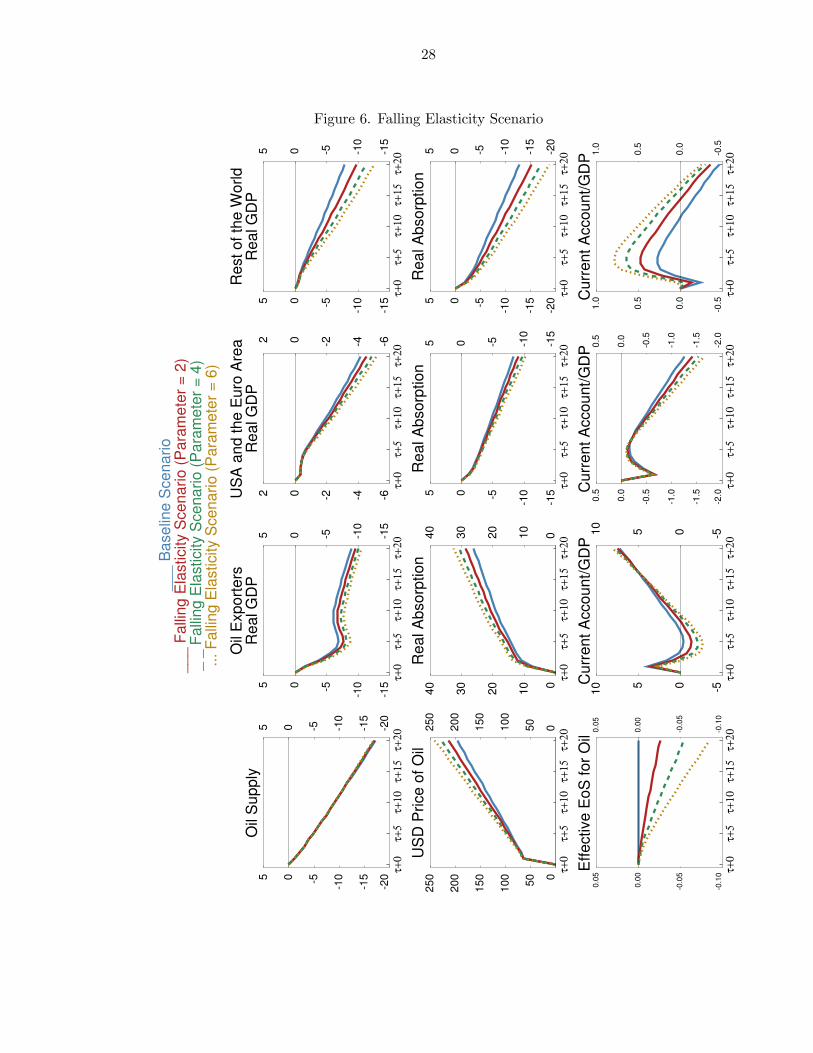
28
Figure 6. Falling Elasticity Scenario
__
_ B
ase
line
Sce
na
rio
__
_ F
alli
ng
Ela
sticity S
ce
na
rio
(P
ara
me
ter
= 2
)_
_ F
alli
ng
Ela
sticity S
ce
na
rio
(P
ara
me
ter
= 4
)..
. F
alli
ng
Ela
sticity S
ce
na
rio
(P
ara
me
ter
= 6
)
-20
-15
-10-505
-20
-15
-10
-505
τ+
0τ+
5τ+
10
τ+
15
τ+
20
Oil
Su
pp
ly
0
50
100
150
200
250
050
100
150
200
250
τ+
0τ+
5τ+
10
τ+
15
τ+
20
US
D P
rice
of
Oil
-0.1
0
-0.0
5
0.0
0
0.0
5
-0.1
0
-0.0
5
0.0
0
0.0
5
τ+
0τ+
5τ+
10
τ+
15
τ+
20
Eff
ective
Eo
S f
or
Oil
-15
-10-505
-15
-10
-505
τ+
0τ+
5τ+
10
τ+
15
τ+
20
Oil
Exp
ort
ers
Re
al G
DP
0
10
20
30
40
010
20
30
40
τ+
0τ+
5τ+
10
τ+
15
τ+
20
Re
al A
bso
rptio
n
-505
10
-50510
τ+
0τ+
5τ+
10
τ+
15
τ+
20
Cu
rre
nt
Acco
un
t/G
DP
-6-4-202
-6-4-202
τ+
0τ+
5τ+
10
τ+
15
τ+
20
US
A a
nd
th
e E
uro
Are
aR
ea
l G
DP
-15
-10-505
-15
-10
-505
τ+
0τ+
5τ+
10
τ+
15
τ+
20
Re
al A
bso
rptio
n
-2.0
-1.5
-1.0
-0.5
0.0
0.5
-2.0
-1.5
-1.0
-0.5
0.0
0.5
τ+
0τ+
5τ+
10
τ+
15
τ+
20
Cu
rre
nt
Acco
un
t/G
DP
-15
-10-505
-15
-10
-505
τ+
0τ+
5τ+
10
τ+
15
τ+
20
Re
st
of
the
Wo
rld
Re
al G
DP
-20
-15
-10-505
-20
-15
-10
-505
τ+
0τ+
5τ+
10
τ+
15
τ+
20
Re
al A
bso
rptio
n
-0.5
0.0
0.5
1.0
-0.5
0.0
0.5
1.0
τ+
0τ+
5τ+
10
τ+
15
τ+
20
Cu
rre
nt
Acco
un
t/G
DP
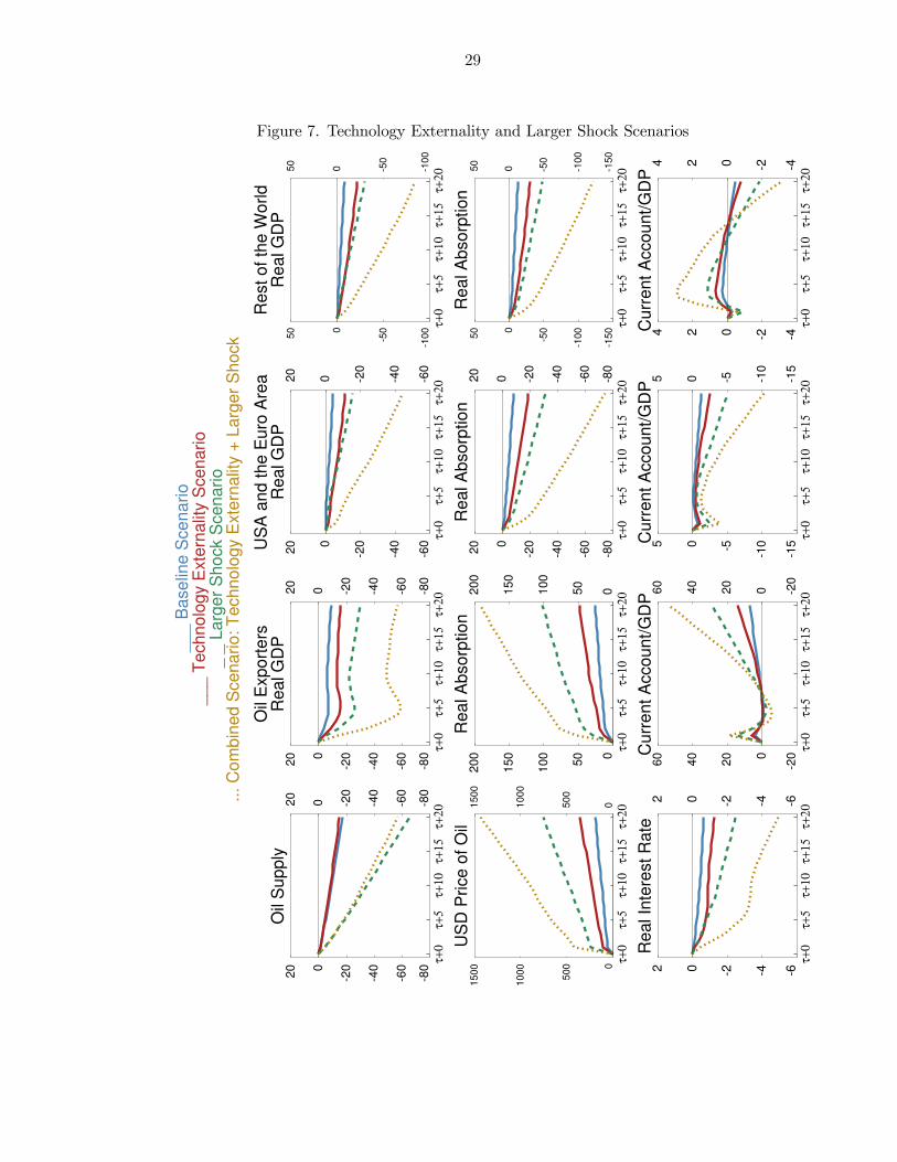
29
Figure 7. Technology Externality and Larger Shock Scenarios
__
_ B
ase
line
Sce
na
rio
__
_ T
ech
no
log
y E
xte
rna
lity S
ce
na
rio
_ _
La
rge
r S
ho
ck S
ce
na
rio
...
Co
mb
ine
d S
ce
na
rio
: T
ech
no
log
y E
xte
rna
lity +
La
rge
r S
ho
ck
-80
-60
-40
-200
20
-80
-60
-40
-20
020
τ+
0τ+
5τ+
10
τ+
15
τ+
20
Oil
Su
pp
ly
0
50
0
10
00
15
00
050
0
10
00
15
00
τ+
0τ+
5τ+
10
τ+
15
τ+
20
US
D P
rice
of
Oil
-6-4-202
-6-4-202
τ+
0τ+
5τ+
10
τ+
15
τ+
20
Re
al In
tere
st
Ra
te
-80
-60
-40
-200
20
-80
-60
-40
-20
020
τ+
0τ+
5τ+
10
τ+
15
τ+
20
Oil
Exp
ort
ers
Re
al G
DP
0
50
100
150
200
050
100
150
200
τ+
0τ+
5τ+
10
τ+
15
τ+
20
Re
al A
bso
rptio
n
-200
20
40
60
-20
020
40
60
τ+
0τ+
5τ+
10
τ+
15
τ+
20
Cu
rre
nt
Acco
un
t/G
DP
-60
-40
-200
20
-60
-40
-20
020
τ+
0τ+
5τ+
10
τ+
15
τ+
20
US
A a
nd
th
e E
uro
Are
aR
ea
l G
DP
-80
-60
-40
-200
20
-80
-60
-40
-20
020
τ+
0τ+
5τ+
10
τ+
15
τ+
20
Re
al A
bso
rptio
n
-15
-10-505
-15
-10
-505
τ+
0τ+
5τ+
10
τ+
15
τ+
20
Cu
rre
nt
Acco
un
t/G
DP
-10
0
-500
50
-10
0
-50
050
τ+
0τ+
5τ+
10
τ+
15
τ+
20
Re
st
of
the
Wo
rld
Re
al G
DP
-15
0
-10
0
-500
50
-15
0
-10
0
-50
050
τ+
0τ+
5τ+
10
τ+
15
τ+
20
Re
al A
bso
rptio
n
-4-2024
-4-2024
τ+
0τ+
5τ+
10
τ+
15
τ+
20
Cu
rre
nt
Acco
un
t/G
DP

30
Figure 8. Combined Downside and Growing Elasticity Scenario
__
_ C
om
bin
ed
Sce
na
rio
: T
ech
no
log
y E
xte
rna
lity +
La
rge
r S
ho
ck
__
_ C
om
bin
ed
Sce
na
rio
: T
ech
no
log
y E
xte
rna
lity +
La
rge
r S
ho
ck +
Gro
win
g E
lasticity (
Pa
ram
ete
r =
1)
_ _
Co
mb
ine
d S
ce
na
rio
: T
ech
no
log
y E
xte
rna
lity +
La
rge
r S
ho
ck +
Gro
win
g E
lasticity (
Pa
ram
ete
r =
2)
-80
-60
-40
-200
20
-80
-60
-40
-20
020
τ+
0τ+
5τ+
10
τ+
15
τ+
20
Oil
Su
pp
ly
0
50
0
10
00
15
00
050
0
10
00
15
00
τ+
0τ+
5τ+
10
τ+
15
τ+
20
US
D P
rice
of
Oil
-6-4-202
-6-4-202
τ+
0τ+
5τ+
10
τ+
15
τ+
20
Re
al In
tere
st
Ra
te
-80
-60
-40
-200
20
-80
-60
-40
-20
020
τ+
0τ+
5τ+
10
τ+
15
τ+
20
Oil
Exp
ort
ers
Re
al G
DP
0
50
100
150
200
050
100
150
200
τ+
0τ+
5τ+
10
τ+
15
τ+
20
Re
al A
bso
rptio
n
-200
20
40
60
-20
020
40
60
τ+
0τ+
5τ+
10
τ+
15
τ+
20
Cu
rre
nt
Acco
un
t/G
DP
-60
-40
-200
20
-60
-40
-20
020
τ+
0τ+
5τ+
10
τ+
15
τ+
20
US
A a
nd
th
e E
uro
Are
aR
ea
l G
DP
-80
-60
-40
-200
20
-80
-60
-40
-20
020
τ+
0τ+
5τ+
10
τ+
15
τ+
20
Re
al A
bso
rptio
n
-15
-10-505
-15
-10
-505
τ+
0τ+
5τ+
10
τ+
15
τ+
20
Cu
rre
nt
Acco
un
t/G
DP
-10
0
-500
50
-10
0
-50
050
τ+
0τ+
5τ+
10
τ+
15
τ+
20
Re
st
of
the
Wo
rld
Re
al G
DP
-15
0
-10
0
-500
50
-15
0
-10
0
-50
050
τ+
0τ+
5τ+
10
τ+
15
τ+
20
Re
al A
bso
rptio
n
-4-2024
-4-2024
τ+
0τ+
5τ+
10
τ+
15
τ+
20
Cu
rre
nt
Acco
un
t/G
DP


