Oil News Sentiment and Volatility in Energy Market · · 2017-05-12Oil News Sentiment and...

1

Oil News Sentiment and Volatility in Energy Market

Song-Zan Chiou-Wei Professor

Department of International Business National Kaohsiung University of Applied Sciences

Kaohsiung, Taiwan

Sheng-Hung Chen Associate Professor

Department of Finance Nanhua University

Chiayi, Taiwan

Zhen Zhu Professor

Department of Economics University of Central Oklahoma

Edmond, OK, USA

March 2017

Abstract

This paper examines the effects of oil news sentiment on both of spot and future returns in energy commodity (crude oil, heating oil, gasoline, and natural gas) using weekly data from September 2006 to August 2016. Specifically, the asymmetric effects of sentiment (pessimism versus optimism) on volatility of spot and future returns in energy commodity are empirically investigated by GARCH (1,1) and DCC-MGARCH, repectively. Our empirical results indicate that based on the univariate GARCH (1,1) model, optimistic sentiment (positive sentiment change) significantly enhances both of spot and futures retunes while showing the robustness as the alternative measure of percentage change in oil news sentiment index. Moreover, the results of multivariate GARCH model using DCC-MGARCH indicates the similar finding that optimistic sentiment economically proliferates both of spot and futures retunes. Besides, optimistic sentiment change significantly mitigates the volatility for spot returns while pessimistic sentiment change only increases the volatility risk of crude oil. Moreover, optimistic sentiment change significantly decreases the volatility for futures return as pessimistic sentiment change conversely increases the volatility risk into crude oil and gasoline.

Keywords: News Sentiment; Volatility Spillover; Energy Market

2

1. Introduction

Considering that the nominal value of the energy commodity futures contracts

traded on the New York Mercantile Exchange (NYMEX) amounts to between 1/3 and

1/2 of the market value of the stocks traded on the New York Stock Exchange (NYSE)

and that energy related products are critically important to our economic system,

understanding what drives the energy prices cannot be under emphasized. As a result the

extreme behavior of energy spot and futures prices in recent years has captured the

attention of hedgers, speculators, regulators and academics alike. Figure 1 presents the

time series of weakly closing settlement prices for the spot energy commodity prices

(crude oil, heating oil, gasoline, and natural gas), obtained from EIA (U.S. Energy

Information Administration) and the corresponding time series of weekly changes in the

log of the spot prices for the period September 2006 to August 2016. Figure 2 presents

the time series of weekly futures prices and changes in the log of the futures prices.

Noticeable in both figures are what appear to be jumps in the data, not to mention

seasonal patterns, portrayed in Figure 3 and 4.

Futures markets are felt to be important aggregators of information about

commodity prices ultimately contributing to the efficient allocation of commodity

resources. Black (1976) goes so far as to argue that this price discovery role of futures

markets dominates its role as a facilitator of risk sharing. Efficient price discovery

however does not necessarily imply ‘smooth’ price changes. When news surprises occur

efficient price discovery will manifest itself as price jumps in much the way Figures 1

and 2 portray. In addition, if price discovery occurs in the futures market (possibly due

to low transactions costs) and is subsequently manifested in the spot market, we should

observe jumps in spot prices but with a lag. Jumps in energy prices are an especially

important element of the market and are an accepted phenomenon. Models of the

dynamics of natural gas and oil prices generally have treated sharp moves in prices as a

generalized jump process with a constant jump parameter (see Clelow and Strickland,

2000; Deng, 2000; Seppi, 2002; and Eydeland and Wolyniec, 2003, for examples and

the references therein). Formal studies of the fundamental determinants of these jumps

however are largely absent from the literature. Understanding how news about the

fundamental determinants of energy prices influences price change shocks is an

3

important element of understanding and modeling the dynamics of energy prices and

jumps in the series. One of our main concerns is on how fundamental changes influence

changes in the levels of the futures prices as well as the spot prices for four energy

commodities : namely, crude oil, heating oil, gasoline, and natural gas.

Also, after studying the futures price data at Commodity Futures Traders

Commission (CFTC), Haigh et al (2007) argued that speculators actually help the gas

market by reducing volatility and increasing liquidity. It is the commercial market

participants such as producers, brokers and trading companies that drive most of the

energy price movements on the New York Mercantile Exchange (NYMEX) where

energy futures contracts are traded. They further suggested that dealers and merchants

(commercial traders or fundamental traders) change their positions first, prompting a

change of positions from hedge funds (speculators) and hedge funds react to price but

not cause it. Haigh et al's comments contradicted those of several others, who asserted

that hedge funds (speculators) are responsible for increasing volatility in both the

futures and cash markets (e.g., Stein, 1987; Hart and Kreps ;1986;Brunetti et al.

2011;Singleton ,2014; Ding et al. ,2014).

Haigh et al (2007) provided more detailed trader profile data for the gas and oil

futures contract traded in NYMEX. Their conclusions mirror those in the above

paragraph. Our proposed study intends to supplement the Haigh et al’s study in two

major areas. Haigh et al used the futures and options data for the period of 8/4/2003 to

8/31/2004, a period that is about 1 year. There is a need to examine a longer time

period since the market composition of the traders has changed substantially, with many

hedge funds, institutional investors and others crowding into the energy markets in

recent years. In addition and more importantly, we will incorporate fundamental

variables in the study to aid our understanding of the behavior of the energy market.

This is particularly important since it will enable us to determine the degree to which

the market follows fundamentals or is driven by market sentiments or speculations.

Recently, a plethora of financial studies had addressed the importance of market

sentiment in determining the asset returns (Riordan, Storkenmaier, Wagener, & Zhang,

2012; Tetlock, 2007, Tetlock, 2010 and Tetlock et al., 2008). Among the authors,

Riordan et al. (2012) indicates that compared with positive news, negative news has

more information contents and exerts substantial impact on asset prices and liquidity.

4

Different scholars also use a wide range of investor sentiment indices to carry out

empirical research. Simon and Wiggins (2001) and Chen and Chang (2005) employed

VIX、put-call ratio and TRIN；Sanders et al. (2003) used Consensus Bullish as a proxy

and Kurov (2008) made use of Individual Investors Sentiment Indicators compiled from

Investor Intelligence and American Association；lastly，Baker and Wurgler, (2006) and

Baker and Wurgler (2007) created their indices based on the investor’s belief of future

asset price and risk. Lee et al. (2002) had found that Investors’ Intelligence sentiment

is a significant factor in determining the stock price returns and fluctuation. The

conclusion is similar to Bahloul and Bouri (2016), who investigated thirteen futures

returns.

In line with market sentiment index, news sentiment, which refers to the

dissemination of news that might shape sentiment, or beliefs of market participants

about the state of the market, is proved to be a key indicator in different financial asset

and commodity price determination (for example, Antweiler and Frank, 2004; Tetlock,

2007 Feuerriegel and Neumann 2013,; Zheng, 2014; Ratku, Feuerriegel, and Neumann,

2014; Feuerriegel, Heitzmann, and Neumann 2015; Borovkova and Mahakena, 2015).

Among them, negative news sentiment is found by Feuerriegel and Neumann (2013) as

a stronger driver in oil and gold market than positive news sentiment. This finding

highlights an important implication that the asymmetric effect of news sentiment should

be included in further examining the price dynamics. Zheng(2014) had successfully put

this perspective into the linkage between stock market investor sentiment and

commodity futures returns. Using VAR-GARCH-M, Zheng found the existence of the

asymmetric response of prices to news.

Though directed toward a similar purpose, this study attempts to compliment

Zheng’s work in three ways. 1) We consider energy commodity of spot and future

returns while Zheng (2014) only focused on the commodity futures returns. 2) We use

the weekly oil news sentiment index different form Zheng (2014) of monthly stock

market investor sentiment, and then empirically and directly investigate sentimental

asymmetry (pessimism versus optimism) on the energy commodity of spot and future

returns. 3) Both of univariate and multivariate GARCH models, are employed for

estimating the volatility clustering and spillovers among the energy markets.

This paper is expected to shed light on the role of news sentiment in price

5

formation and volatility formation, which would lead to more efficient market

regulation and oversight and efficiency improvement. In doing so, we intend to

disentangle the puzzle of the news sentiment, and lastly, empirical evidence of cross

market linkages is scarce in the co-movement correlation literature. This result, however,

is warranted since there are implications for diversification benefits associated with it.

We investigate four energy price return correlations using a multivariate setting.

2. Methodology and Data

To gauge the magnitude of the price change and volatilities, tabular account of

the weekly price changes and volatility in the form of standard deviation (we will also

perform an array of diagnoses of heterogeneity in the standard deviations, and if the

conditional heterogeneity holds true, the GARCH model estimation of the volatility

would be added,) and coefficient of variation will be provided. Week to week price

change as well as weekly average price changes by year, season and for the whole

sample period will be calculated to show the magnitudes of price fluctuations. Below

delineates three basic specifications regarding our research questions.

2.1 Univariate GARCH

This paper used the GARCH model to capture the volatility clustering in

energ market, including contemporaneous shifts in oil news sentiment in the mean

equation and lagged shifts in the magnitude of investor sentiment in the conditional

volatility equation. Therefore, our model is specified as GARCH (1,1) with the

following form:

2 3

, 0 1 , , , ,1 1

, (0, )i t t j i t j k t i t i t i tj k

RET Sent RET SEA h

(1)

2 2 2, 0 1 , 1 2 , 1 3 1 1 4 1 1( ) ( )i t i t i t t t t th h Sent D Sent D

(2)

where RETi,t is the weekly return on an energy commodity (crude oil, heating oil,

gasoline, and natural gas), Sentt is a weekly measure of oil headline news index

6

monitored by sentix (www.sentix.de), which is based on a survey-based index

calculated from a market assessment of 5000 registered investors from Europe, the USA,

and Japan. Specifically, two alternative measures of sentiment index are used in

Equation (1). The first measure is calculated as the change in the oil news sentiment

index, ΔSentt=Sentt-Sentt-1; the second is measured as the percentage change in oil news

sentiment index, %ΔSentt=ΔSentt/Sentt-1. SEAt represents the month effect with higher

returns for four energy commodity and the includes three seasonal dummies on

February, March, and April. In Equation (2), 1 1tD if ΔSentt>0; otherwise, 1 0tD

if ΔSentt 0 .

2.2 Multivariate GARCH (DCC-MGARCH)

We estimate a dynamic conditional correlation (DCC-MGARCH) model,

which is flexible enough to account for its own and cross-market volatility and

persistence across the markets. In addition, the DCC model provides a dynamic

conditional correlation matrix, which enables us to study whether the cross market

interdependence is time-varying or not. Therefore, we model the price behavior as the

following model:

3

0 1 11 1

, (0, )k

t t j t j k t t t t tj k

RET Sent RET SEA I H

(3)

where tRET is a 4 × 1 vector of returns for crude oil, heating oil, gasoline and natural

gas, 0 is defined as a 4 × 1 vector of long-term drifts, j , with j = 1,.., k, are 4 × 4

parameter matrices, and t is a 4 × 1 vector of forecast errors for the best linear

predictor of tRET . The forecast error is conditional on past information ( 1tI ), and the

error has a corresponding variance–covariance matrix tH . The elements of j , j=1,.., k,

provide measures of own- and cross-mean spillovers between markets as in a standard

VAR representation.

We define the conditional variance-covariance matrix tH as

7

2 21 1 1 1 1 1 2 1 1( ) ( )t t t t t t t tH C C A A G H G Sent D Sent D (4)

where C is a 4 × 4 upper triangular matrix of constants ijC , A is a 4 × 4 matrix

containing elements ijA that measure the degree of innovation from market i to market

j, and G is a 4 × 4 matrix whose elements ijG show the persistence in conditional

volatility between markets i and j. The conditional variance–covariance matrix as we

defined in Eq. (4) allows us to study the volatility transmission across markets in terms

of its persistence, direction and magnitude.

A DCC model assumes a time-dependent conditional correlation matrix

RETt=(ρij,t), i, j = 1, …, 4, and the conditional variance–covariance matrix Ht

t t t tH D R D (5)

where

11, 33,,.....,t t tD diag h h (6)

,ii th is assumed to follow a GARCH(1,1) specification, i.e. 2, , 1 ,ii t i i i t i ii th h , i =

1,…, 4, and

1/2 1/2, ,t ii t t ii tRET diag q Q diag q (7)

with the 4 × 4 symmetric positive-definite matrix Qt = (qij,t), i, j = 1,…, 4, given by

1 2 1 1 1 2 1(1 )t t t tQ Q u u Q (8)

and ,/it it ii tu h Q is the 4 × 4 unconditional variance matrix of tu , and 1 and

2 are non-negative adjustment parameters satisfying 0< 1 + 2 <1.

8

2.3 Data

The weekly measure on investor sentiment of oil headline news index is

mainly collected from Sentix (www.sentix.de), based on a survey-based index

calculated from a market assessment of 5000 registered investors from Europe, the USA,

and Japan. Both of spot and future prices for energy commodities, including crude oil,

heating oil, gasoline, and natural gas, are obtained from EIA (U.S. Energy Information

Administration) (www.eia.gov). Our weekly data spans from September 2006 to August

2016.

3. Empirical Results

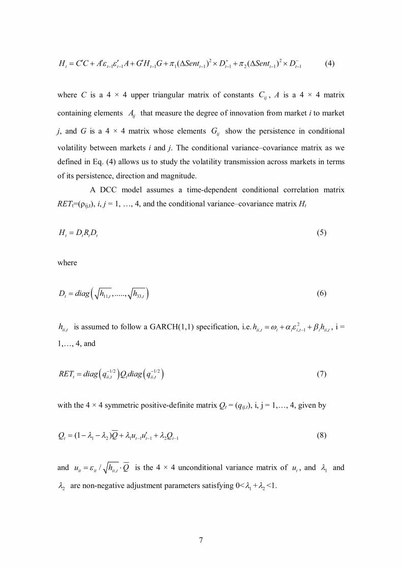
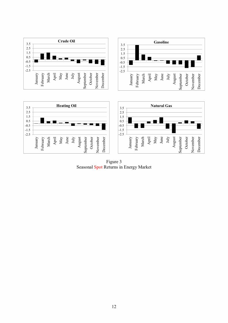
Both of spot and futures returns on energy commodity present the

co-movement pattern with time (Figure 1 & 2). As shown in Figure 3 & 4, seasonal spot

and futures returns in energy market exhibited higher averaged returns in three months

of February, March, and April. Based on this observation, we control for seasonal fixed

effect in our specification of mean equation.

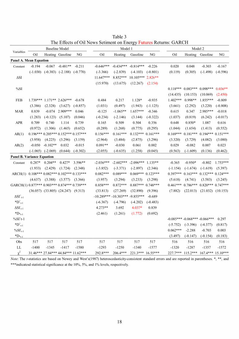
3.1 The effects of change in oil news sentiment on spot and futures returns

Based on the univariate GARCH (1,1) model, optimistic sentiment (positive

sentiment change) significantly enhances both of spot and futures retunes. This result

also shows the robustness as the alternative measure of percentage change in oil news

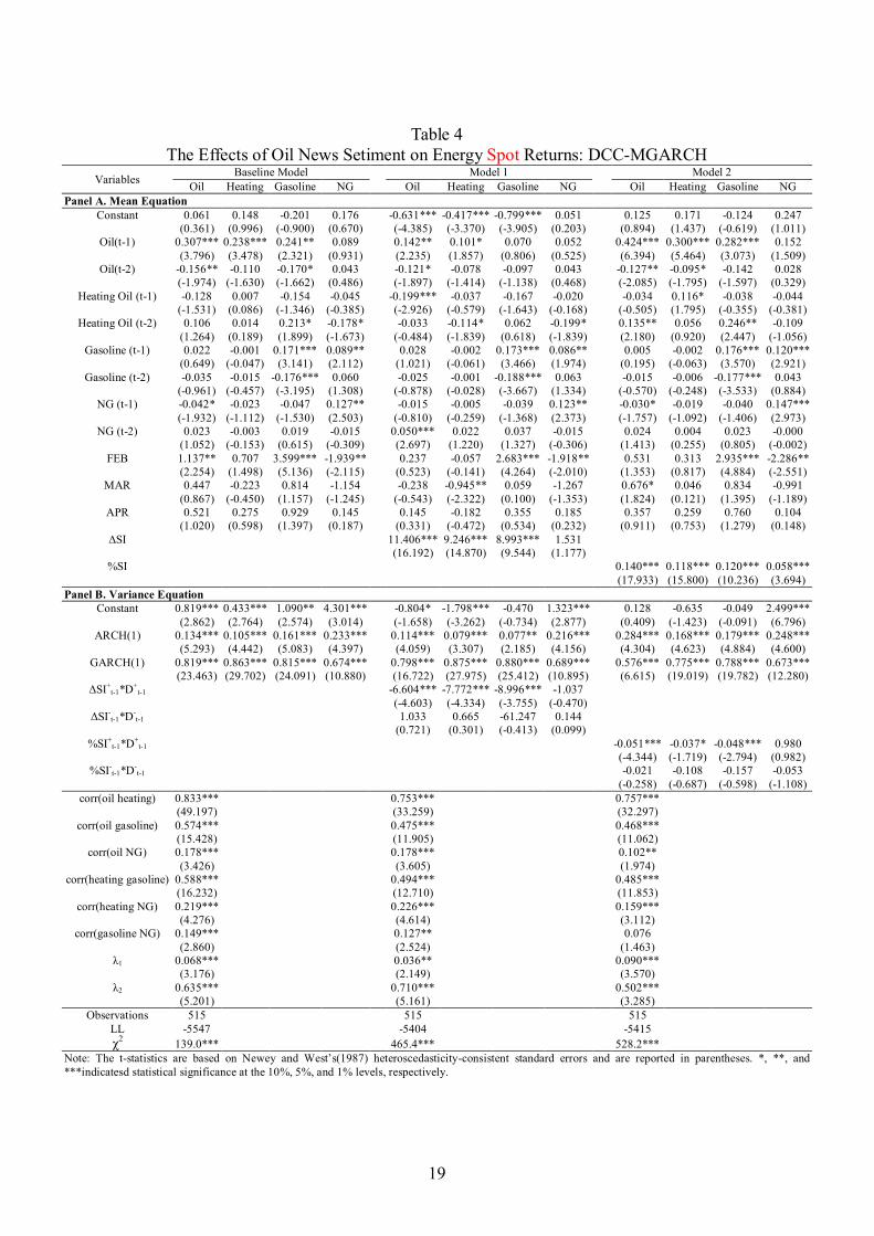
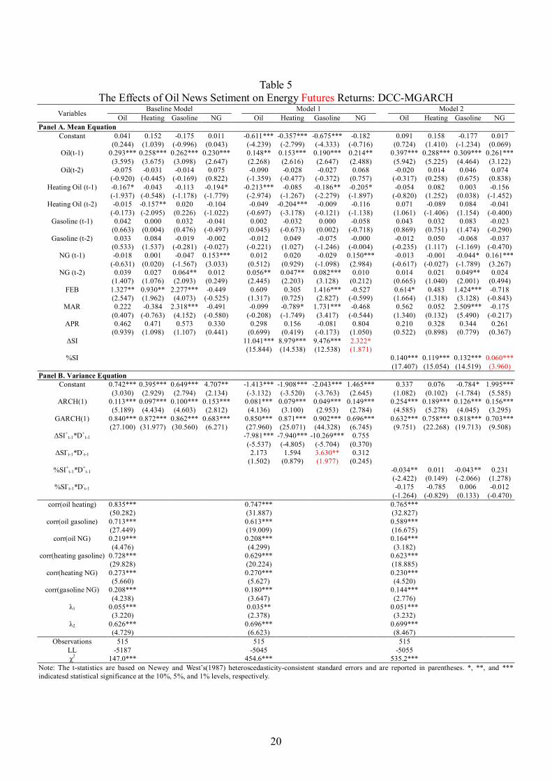
sentiment index. The results of multivariate GARCH model using DCC-MGARCH

indicates the similar finding that optimistic sentiment economically proliferates both

of spot and futures retunes.

3.2 The asymmetric effects of change in oil news sentiment on spot and futures

volatilities

First, based on univariate GARCH model, optimistic sentiment change

significantly mitigates the volatility for spot returns while pessimistic sentiment change

9

only increases the volatility risk of crude oil. Moreover, optimistic sentiment change

significantly decreases the volatility for futures return as pessimistic sentiment change

conversely increases the volatility risk into crude oil and gasoline. Second, based on the

DCC-MGARCH, optimistic sentiment change maintains the positive influence on

reducing volatilities for spot returns while this effect present consistent in futures

returns for all commodities. We find the significance in volatility dynamics and

spillovers cross market. The correlation among all commodities shows the significance

in futures returns.

4. Conclusion

This paper discovers the asymmetrical impacts of news sentiment, the final

results can aid investors to evaluate the timing of investment in order to avoid problems

associated with irrational exuberance. Also, the government can utilize the news

sentiment as a beacon for market stabilization policy and risk control. However, crude

oil, heating oil, gasoline, and natural gas are four major energy substitute products, as

we know. The cross market volatility spillover effect is found from the results of

multivariate GARCH, the market participants can accordingly calculate the optimal

hedge ratio and portfolio weight for the diversification.

We show that based optimistic sentiment (positive sentiment change)

significantly enhances both of spot and futures retunes while showing the robustness as

the alternative measure of percentage change in oil news sentiment index. while

multivariate model indicates the similar finding that optimistic sentiment economically

proliferates both of spot and futures retunes. inaddition, optimistic sentiment change

significantly mitigates the volatility for spot returns while pessimistic sentiment change

only increases the volatility risk of crude oil. Finally, optimistic sentiment change

significantly decreases the volatility for futures return as pessimistic sentiment change

conversely increases the volatility risk into crude oil and gasoline.

10

A1. Crude Oil Price A2. Crude Oil Returns

B1. Heating Oil Price B2. Heating Oil Returns

C1. Gasoline Price C2. Gasoline Returns

D1. Natural Gas Price D2. Natural Gas Returns

Figure 1 Oil News Sentitment and Spot Price (Returns) of Energy Commodity

-.4-.2

0.2

.4.6 O

il N

ews

Sen

timen

t Ind

ex

2040

6080

100

120

140

Oil

Spo

t Pric

e

01jan2006 01jan2008 01jan2010 01jan2012 01jan2014 01jan2016

Date

Oil Spot Price Oil News Sentiment Index

-.4-.2

0.2

.4.6 O

il N

ews

Sen

timen

t Ind

ex

-20

-10

010

2030

Oil

Spo

t Ret

urns


Date

Oil Spot Returns Oil News Sentiment Index

-.4-.2

0.2

.4.6

Oil

New

s S

entim

ent I

ndex

11.

52

2.5

33.

54

Hea

ting

Oil

Spot

Pric

e


Date

Heating Oil Spot Price Oil News Sentiment Index

-.4-.2

0.2

.4.6

Oil

New

s S

entim

ent I

ndex

-20

-10

010

20H

eatin

g O

il S

pot R

etur

ns


Date

Heating Oil Spot Returns Oil News Sentiment Index

-.4-.2

0.2

.4.6

Oil

New

s Se

ntim

ent I

ndex

.51

1.5

22.

53

3.5

4

Gas

olin

e Sp

ot P

rice


Date

Gasoline Spot Price Oil News Sentiment Index

-.4-.2

0.2

.4.6

Oil

New

s Se

ntim

ent I

ndex

-40

-20

020

40G

asol

ine

Spo

t Ret

urns

01jan2006 01jan2008 01jan2010 01jan2012 01jan2014 01jan2016Date

Gasoline Spot Returns Oil News Sentiment Index

-.4-.2

0.2

.4.6

Oil

New

s S

entim

ent I

ndex

23

45

67

89

1011

1213

Nat

ural

Gas

Spo

t Pric

e


Date

Natural Gas Spot Price Oil News Sentiment Index

-.4-.2

0.2

.4.6 O

il N

ews

Sen

timen

t Ind

ex

-40

-20

020

40N

atur

al G

as S

pot R

etur

ns


Natural Gas Spot Returns Oil News Sentiment Index

11

A1. Crude Oil Price A2. Crude Oil Returns

B1. Heating Oil Price B2. Heating Oil Returns

C1. Gasoline Price C2. Gasoline Returns

D1. Natural Gas Price D2. Natural Gas Returns

Figure 2 Oil News Sentitment and Futures Price (Returns) of Energy Commodity

-.4-.2

0.2

.4.6 O

il N

ews

Sen

timen

t Ind

ex

2040

6080

100

120

140

Oil

Futu

res

Pric

e


Date

Oil Futures Price Oil News Sentiment Index

-.4-.2

0.2

.4.6 O

il N

ews

Sen

timen

t Ind

ex

-20

-10

010

20O

il Fu

ture

s R

etur

ns


Date

Oil Futures Returns Oil News Sentiment Index

-.4-.2

0.2

.4.6

Oil

New

s Se

ntim

ent I

ndex

11.

52

2.5

33.

54

Hea

ting

Oil

Futu

res

Pric

e


Date

heating_oil_futures_pe1 Oil News Sentiment Index

-.4-.2

0.2

.4.6

Oil

New

s S

entim

ent I

ndex

-20

-10

010

20H

eatin

g O

il Fu

ture

s R

etur

ns


Heating Oil Futures Returns Oil News Sentiment Index

-.4-.2

0.2

.4.6 O

il N

ews

Sen

timen

t Ind

ex

11.

52

2.5

33.

5G

asol

ine

Futu

res

Pric

e


Date

Gasoline Futures Price Oil News Sentiment Index

-.4-.2

0.2

.4.6 O

il N

ews

Sen

timen

t Ind

ex

-20

-10

010

20G

asol

ine

Futu

res

Ret

urns


Date

Gasoline Futures Returns Oil News Sentiment Index

-.4-.2

0.2

.4.6 O

il N

ews

Sen

timen

t Ind

ex

05

1015

Nat

ural

Gas

Fut

ures

Pric

e


DateNatural Gas Futures Price Oil News Sentiment Index

-.4-.2

0.2

.4.6

Oil

New

s S

entim

ent I

ndex

-20

-10

010

20N

atur

al G

as F

utur

es R

etur

ns


Date

Natural Gas Futures Returns Oil News Sentiment Index

12

Figure 3 Seasonal Spot Returns in Energy Market

-2.5-1.5-0.50.51.52.53.5

Janu

ary

Febr

uary

Mar

chA

pril

May

June

July

Aug

ust

Sept

embe

rO

ctob

erN

ovem

ber

Dec

embe

r

Crude Oil

-2.5-1.5-0.50.51.52.53.5

Janu

ary

Febr

uary

Mar

chA

pril

May

June

July

Aug

ust

Sept

embe

rO

ctob

erN

ovem

ber

Dec

embe

r

Gasoline

-2.5-1.5-0.50.51.52.53.5

Janu

ary

Febr

uary

Mar

chA

pril

May

June

July

Aug

ust

Sept

embe

rO

ctob

erN

ovem

ber

Dec

embe

rHeating Oil

-2.5-1.5-0.50.51.52.53.5

Janu

ary

Febr

uary

Mar

chA

pril

May

June

July

Aug

ust

Sept

embe

rO

ctob

erN

ovem

ber

Dec

embe

r

Natural Gas

13

Figure 4 Seasonal Futures Returns in Energy Market

-2.5-1.5-0.50.51.52.53.5

Janu

ary

Febr

uary

Mar

chA

pril

May

June

July

Aug

ust

Sept

embe

rO

ctob

erN

ovem

ber

Dec

embe

r

Crude Oil

-2.5-1.5-0.50.51.52.53.5

Janu

ary

Febr

uary

Mar

chA

pril

May

June

July

Aug

ust

Sept

embe

rO

ctob

erN

ovem

ber

Dec

embe

r

Gasoline

-2.5-1.5-0.50.51.52.53.5

Janu

ary

Febr

uary

Mar

chA

pril

May

June

July

Aug

ust

Sept

embe

rO

ctob

erN

ovem

ber

Dec

embe

rHeating Oil

-2.5-1.5-0.50.51.52.53.5

Janu

ary

Febr

uary

Mar

chAp

rilM

ayJu

neJu

lyAu

gust

Sept

embe

rOc

tobe

rN

ovem

ber

Dece

mbe

r

Natural Gas

14

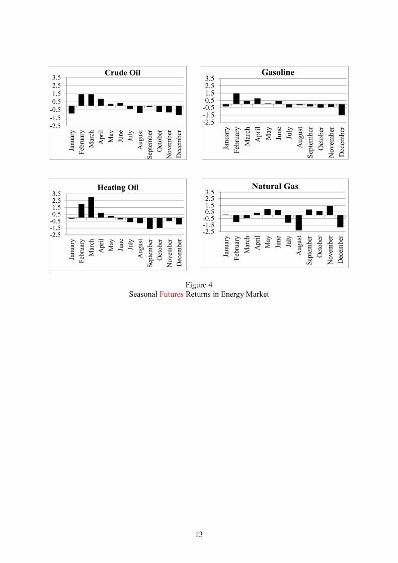
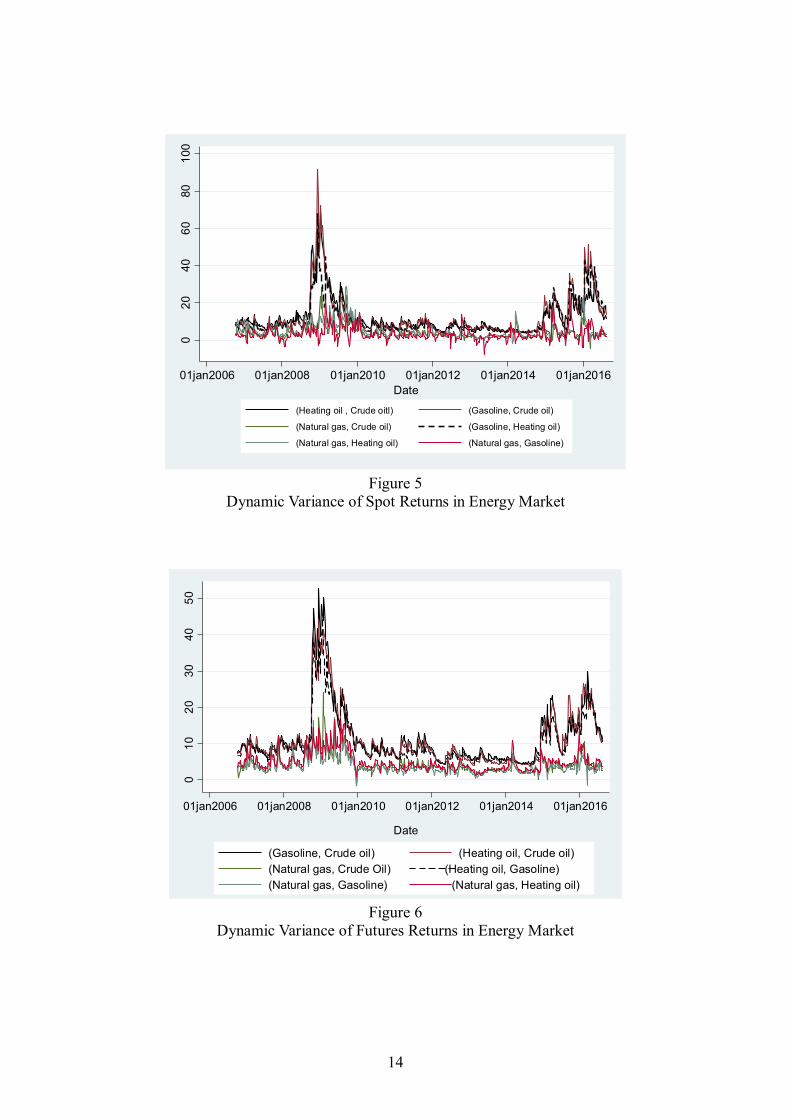
Figure 5

Dynamic Variance of Spot Returns in Energy Market

Figure 6

Dynamic Variance of Futures Returns in Energy Market

020

4060

8010

0


(Heating oil , Crude oitl) (Gasoline, Crude oil)

(Natural gas, Crude oil) (Gasoline, Heating oil)

(Natural gas, Heating oil) (Natural gas, Gasoline)

010

2030

4050


Date

(Gasoline, Crude oil) (Heating oil, Crude oil)(Natural gas, Crude Oil) (Heating oil, Gasoline)(Natural gas, Gasoline) (Natural gas, Heating oil)

15

Figure 7

Dynamic Correlation of Spot Returns in Energy Market

Figure 8

Dynamic Correlation of Ftures Returns in Energy Market

-.20

.2.4

.6.8


(Heating oil, Crude oil) (Gasoline, Crude oil)(Natural gas, Crude oil) (Gasolinet, Heating oil)(Natural gas, Heating oil) (Natural gas, gasoine)

0.2

.4.6

.8


(Gasoline, Crude oil) (Heating oil, Crude oil)(Natural gas, Crude Oil) (Heating oil, Gasoline)(Natural gas, Gasoline) (Natural gas, Heating oil)

16

Table 1 Summary statistics of price, returns, and sentiment index

Variables Observations Mean Standard deviation Minimum Maximum

Panel A. Spot price Cride oil (WTC) 518 79.135 23.241 28.140 142.520

Heating oil 518 2.320 0.696 0.871 3.992 Gasoline 518 2.403 0.614 0.738 3.761

Natural gas 518 4.529 2.125 1.570 13.200 Crude oil returns 517 -0.076 4.449 -19.100 25.125

Heating oil returns 517 -0.059 3.813 -13.155 14.490 Gasoline returns 517 -0.065 6.393 -30.994 34.303

Natural gas returns 517 -0.120 6.502 -30.928 30.099 Panel B. Futures price

Cride oil (WTC) 518 79.218 23.159 28.150 142.460 Heating oil 518 2.360 0.681 0.917 4.006 Gasoline 518 2.271 0.629 0.845 3.534

Natural gas 518 4.588 2.141 1.687 13.456 Crude oil returns 517 -0.076 4.239 -18.723 15.527

Heating oil returns 517 -0.049 3.737 -13.394 12.775 Gasoline returns 517 -0.035 4.354 -17.639 22.037

Natural gas returns 517 -0.137 5.349 -19.774 21.842 Panel C. Oil news sentiment index

Changes in sentiment index 518 0.049 0.197 -0.443 0.565 % Changes in sentiment index 517 0.059 14.894 -55.720 44.800

17

Table 2 The Effects of Oil News Setiment on Energy Spot Returns: GARCH

Variables Baseline Model

Model 1

Model 2

Oil Heating Gasoline NG Oil Heating Gasoline NG Oil Heating Gasoline NG Panel A. Mean Equation

Constant -0.155 -0.049 -0.420* -0.067 -0.656*** -0.441*** -0.948*** -0.084 0.072 0.082 -0.234 0.027

(-0.839) (-0.273) (-1.687) (-0.236) (-3.548) (-2.685) (-4.163) (-0.290) (0.412) (0.491) (-1.031) (0.092)

ΔSI 11.898*** 9.514*** 8.397*** 1.780

(16.051) (14.413) (8.004) (1.349)

%SI 0.118*** 0.085*** 0.088*** 0.026*

(13.666) (10.640) (6.689) (1.767)

FEB 1.664*** 1.053** 4.355*** -1.099 0.460 -0.007 3.210*** -1.355 1.295*** 0.866** 3.794*** -1.360

(3.075) (2.063) (4.133) (-1.021) (0.941) (-0.016) (3.704) (-1.242) (3.200) (1.985) (4.212) (-1.208)

MAR 0.906 -0.025 1.138 -0.443 -0.097 -1.110** 0.042 -0.700 0.731 0.288 0.955 -0.482

(1.461) (-0.041) (1.266) (-0.426) (-0.183) (-2.112) (0.055) (-0.668) (1.290) (0.631) (1.076) (-0.447)

APR 0.615 0.386 1.251 0.639 0.152 -0.101 0.357 0.410 0.554 0.531 1.278 0.581

(0.839) (0.638) (1.239) (0.516) (0.256) (-0.257) (0.436) (0.334) (0.924) (0.980) (1.486) (0.506)

AR(1) 0.201*** 0.234*** 0.206*** 0.152*** 0.155*** 0.198*** 0.194*** 0.163*** 0.180*** 0.216*** 0.207*** 0.158***

(4.004) (4.908) (4.290) (2.911) (2.988) (4.147) (4.259) (3.065) (3.425) (4.360) (4.342) (2.946)

AR(2) -0.084* -0.086* -0.126*** -0.033 0.063 -0.010 -0.135*** -0.034 -0.006 -0.059 -0.155*** -0.027

(-1.770) (-1.795) (-2.643) (-0.711) (1.325) (-0.231) (-2.919) (-0.693) (-0.120) (-1.212) (-3.084) (-0.576)

Panel B. Variance Equation Constant 0.349** 0.159* 1.038*** 4.310*** -1.416*** -2.924*** -1.017* 1.141** -0.170 -0.949* -0.084 2.197***

(2.056) (1.786) (2.740) (2.807) (-2.919) (-3.176) (-1.848) (2.572) (-0.580) (-1.683) (-0.118) (6.125)

ARCH(1) 0.116*** 0.084*** 0.142*** 0.225*** 0.112*** 0.079*** 0.063*** 0.206*** 0.389*** 0.153*** 0.164*** 0.233***

(5.003) (3.568) (4.741) (4.509) (4.255) (3.161) (3.125) (4.561) (5.624) (4.600) (4.682) (4.562)

GARCH(1) 0.867*** 0.906*** 0.829*** 0.678*** 0.808*** 0.891*** 0.885*** 0.700*** 0.449*** 0.799*** 0.799*** 0.678***

(34.888) (38.222) (26.786) (9.713) (23.043) (31.276) (38.280) (10.835) (7.690) (22.018) (23.360) (10.858)

ΔSI+t-1

*D+t-1

-9.170*** -10.947*** -10.991*** -2.632** (-6.463) (-4.338) (-5.794) (-2.021)

ΔSI-t-1

*D-t-1 3.491** 3.358 -1.657 0.746 (2.177) (0.886) (-0.434) (0.500)

%SI+t-1 *D+

t-1 -0.084*** -0.064*** -0.054** 1.259 (-5.716) (-3.121) (-2.207) (0.471)

%SI-t-1

*D-t-1 0.053*** -2.494 -0.222 -0.014 (2.851) (-0.140) (-0.239) (-0.572)

Obs 517 517 517 517 517 517 517 517 516 516 516 516 LL -1412 -1352 -1580 -1648 -1307 -1256 -1532 -1647 -1333 -1293 -1549 -1640 χ2 30.63*** 31.08*** 39.37*** 9.77*** 282.50*** 226.61*** 107.11*** 12.84*** 203.41*** 127.51*** 100.81*** 11.89***

Note: The t-statistics are based on Newey and West’s(1987) heteroscedasticity-consistent standard errors and are reported in parentheses. *, **, and ***indicatesd statistical significance at the 10%, 5%, and 1% levels, respectively.

18

Table 3 The Effects of Oil News Setiment on Energy Futures Returns: GARCH

Variables Baseline Model

Model 1

Model 2

Oil Heating Gasoline NG Oil Heating Gasoline NG Oil Heating Gasoline NG Panel A. Mean Equation

Constant -0.194 -0.067 -0.481** -0.211 -0.646*** -0.434*** -0.814*** -0.226 0.020 0.048 -0.303 -0.167

(-1.030) (-0.383) (-2.188) (-0.770) (-3.366) (-2.839) (-4.103) (-0.801) (0.119) (0.305) (-1.498) (-0.596)

ΔSI 11.647*** 8.852*** 10.105*** 2.826**

(15.970) (13.675) (12.267) (2.154)

%SI 0.118*** 0.083*** 0.098*** 0.036**

(14.435) (10.153) (10.069) (2.450)

FEB 1.739*** 1.171** 2.626*** -0.678 0.484 0.217 1.128* -0.935 1.402*** 0.998** 1.855*** -0.809

(3.386) (2.328) (3.627) (-0.857) (1.031) (0.497) (1.943) (-1.125) (3.661) (2.292) (3.220) (-0.808)

MAR 0.839 -0.074 2.909*** 0.046 -0.125 -1.065** 1.657*** -0.346 0.615 0.347 2.985*** -0.018

(1.283) (-0.123) (5.107) (0.046) (-0.234) (-2.146) (3.144) (-0.322) (1.037) (0.819) (6.242) (-0.017)

APR 0.709 0.740 1.114 0.739 0.165 0.509 0.504 0.356 0.648 0.850* 1.087 0.616

(0.972) (1.306) (1.465) (0.652) (0.289) (1.268) (0.775) (0.295) (1.044) (1.654) (1.413) (0.552)

AR(1) 0.196*** 0.205*** 0.152*** 0.157*** 0.156*** 0.161*** 0.132*** 0.161*** 0.169*** 0.181*** 0.194*** 0.151***

(3.958) (4.225) (3.296) (3.159) (2.964) (3.484) (2.875) (3.296) (3.320) (3.729) (4.082) (3.080)

AR(2) -0.050 -0.102** 0.032 -0.015 0.091** -0.030 0.061 0.002 0.029 -0.082 0.007 0.023

(-1.065) (-2.069) (0.644) (-0.302) (2.055) (-0.635) (1.258) (0.045) (0.563) (-1.609) (0.136) (0.462)

Panel B. Variance Equation Constant 0.287* 0.204** 0.427* 3.596** -2.036*** -2.602*** -2.096*** 1.135** -0.365 -0.950* -0.802 1.753***

(1.933) (2.429) (1.724) (2.348) (-3.852) (-3.371) (-2.897) (2.346) (-1.154) (-1.674) (-1.619) (5.397)

ARCH(1) 0.108*** 0.082*** 0.102*** 0.133*** 0.082*** 0.089*** 0.069*** 0.123*** 0.397*** 0.163*** 0.132*** 0.124***

(4.637) (3.388) (3.577) (3.366) (3.957) (3.294) (3.233) (3.298) (5.618) (4.741) (3.583) (3.245)

GARCH(1) 0.877*** 0.903*** 0.874*** 0.739*** 0.858*** 0.872*** 0.887*** 0.748*** 0.461*** 0.786*** 0.820*** 0.747***

(36.057) (33.805) (24.247) (9.313) (33.813) (27.269) (32.890) (9.396) (7.882) (22.013) (21.032) (10.153)

ΔSI+t-1

*D+t-1

-10.289*** -10.303*** -9.855*** -0.689 (-6.367) (-4.796) (-4.202) (-0.483)

ΔSI-t-1

*D-t-1 4.273** 3.692 4.037* 0.839 (2.461) (1.261) (1.772) (0.692)

%SI+t-1 *D+

t-1 -0.085*** -0.068*** -0.066*** 0.297 (-5.752) (-3.396) (-4.377) (0.817)

%SI-t-1

*D-t-1 0.062*** -2.288 -0.703 0.003 (3.497) (-0.147) (-0.154) (0.183)

Obs 517 517 517 517 517 517 517 517 516 516 516 516 LL -1400 -1345 -1417 -1580 -1293 -1250 -1340 -1577 -1320 -1287 -1357 -1572 χ2 31.46*** 27.84*** 44.84*** 11.62*** 292.8*** 206.4*** 221.3*** 16.55*** 227.7*** 115.2*** 167.4*** 15.10***


19

Table 4 The Effects of Oil News Setiment on Energy Spot Returns: DCC-MGARCH

Variables Baseline Model Model 1 Model 2 Oil Heating Gasoline NG Oil Heating Gasoline NG Oil Heating Gasoline NG

Panel A. Mean Equation Constant 0.061 0.148 -0.201 0.176 -0.631*** -0.417*** -0.799*** 0.051 0.125 0.171 -0.124 0.247

(0.361) (0.996) (-0.900) (0.670) (-4.385) (-3.370) (-3.905) (0.203) (0.894) (1.437) (-0.619) (1.011) Oil(t-1) 0.307*** 0.238*** 0.241** 0.089 0.142** 0.101* 0.070 0.052 0.424*** 0.300*** 0.282*** 0.152

(3.796) (3.478) (2.321) (0.931) (2.235) (1.857) (0.806) (0.525) (6.394) (5.464) (3.073) (1.509) Oil(t-2) -0.156** -0.110 -0.170* 0.043 -0.121* -0.078 -0.097 0.043 -0.127** -0.095* -0.142 0.028

(-1.974) (-1.630) (-1.662) (0.486) (-1.897) (-1.414) (-1.138) (0.468) (-2.085) (-1.795) (-1.597) (0.329) Heating Oil (t-1) -0.128 0.007 -0.154 -0.045 -0.199*** -0.037 -0.167 -0.020 -0.034 0.116* -0.038 -0.044

(-1.531) (0.086) (-1.346) (-0.385) (-2.926) (-0.579) (-1.643) (-0.168) (-0.505) (1.795) (-0.355) (-0.381) Heating Oil (t-2) 0.106 0.014 0.213* -0.178* -0.033 -0.114* 0.062 -0.199* 0.135** 0.056 0.246** -0.109

(1.264) (0.189) (1.899) (-1.673) (-0.484) (-1.839) (0.618) (-1.839) (2.180) (0.920) (2.447) (-1.056) Gasoline (t-1) 0.022 -0.001 0.171*** 0.089** 0.028 -0.002 0.173*** 0.086** 0.005 -0.002 0.176*** 0.120***

(0.649) (-0.047) (3.141) (2.112) (1.021) (-0.061) (3.466) (1.974) (0.195) (-0.063) (3.570) (2.921) Gasoline (t-2) -0.035 -0.015 -0.176*** 0.060 -0.025 -0.001 -0.188*** 0.063 -0.015 -0.006 -0.177*** 0.043

(-0.961) (-0.457) (-3.195) (1.308) (-0.878) (-0.028) (-3.667) (1.334) (-0.570) (-0.248) (-3.533) (0.884) NG (t-1) -0.042* -0.023 -0.047 0.127** -0.015 -0.005 -0.039 0.123** -0.030* -0.019 -0.040 0.147***

(-1.932) (-1.112) (-1.530) (2.503) (-0.810) (-0.259) (-1.368) (2.373) (-1.757) (-1.092) (-1.406) (2.973) NG (t-2) 0.023 -0.003 0.019 -0.015 0.050*** 0.022 0.037 -0.015 0.024 0.004 0.023 -0.000

(1.052) (-0.153) (0.615) (-0.309) (2.697) (1.220) (1.327) (-0.306) (1.413) (0.255) (0.805) (-0.002) FEB 1.137** 0.707 3.599*** -1.939** 0.237 -0.057 2.683*** -1.918** 0.531 0.313 2.935*** -2.286**

(2.254) (1.498) (5.136) (-2.115) (0.523) (-0.141) (4.264) (-2.010) (1.353) (0.817) (4.884) (-2.551) MAR 0.447 -0.223 0.814 -1.154 -0.238 -0.945** 0.059 -1.267 0.676* 0.046 0.834 -0.991

(0.867) (-0.450) (1.157) (-1.245) (-0.543) (-2.322) (0.100) (-1.353) (1.824) (0.121) (1.395) (-1.189) APR 0.521 0.275 0.929 0.145 0.145 -0.182 0.355 0.185 0.357 0.259 0.760 0.104

(1.020) (0.598) (1.397) (0.187) (0.331) (-0.472) (0.534) (0.232) (0.911) (0.753) (1.279) (0.148) ΔSI 11.406*** 9.246*** 8.993*** 1.531

(16.192) (14.870) (9.544) (1.177) %SI 0.140*** 0.118*** 0.120*** 0.058***

(17.933) (15.800) (10.236) (3.694) Panel B. Variance Equation

Constant 0.819*** 0.433*** 1.090** 4.301*** -0.804* -1.798*** -0.470 1.323*** 0.128 -0.635 -0.049 2.499*** (2.862) (2.764) (2.574) (3.014) (-1.658) (-3.262) (-0.734) (2.877) (0.409) (-1.423) (-0.091) (6.796)

ARCH(1) 0.134*** 0.105*** 0.161*** 0.233*** 0.114*** 0.079*** 0.077** 0.216*** 0.284*** 0.168*** 0.179*** 0.248*** (5.293) (4.442) (5.083) (4.397) (4.059) (3.307) (2.185) (4.156) (4.304) (4.623) (4.884) (4.600)

GARCH(1) 0.819*** 0.863*** 0.815*** 0.674*** 0.798*** 0.875*** 0.880*** 0.689*** 0.576*** 0.775*** 0.788*** 0.673*** (23.463) (29.702) (24.091) (10.880) (16.722) (27.975) (25.412) (10.895) (6.615) (19.019) (19.782) (12.280)

ΔSI+t-1*D+

t-1 -6.604*** -7.772*** -8.996*** -1.037 (-4.603) (-4.334) (-3.755) (-0.470)

ΔSI-t-1*D-

t-1 1.033 0.665 -61.247 0.144 (0.721) (0.301) (-0.413) (0.099)

%SI+t-1*D+

t-1 -0.051*** -0.037* -0.048*** 0.980 (-4.344) (-1.719) (-2.794) (0.982)

%SI-t-1*D-

t-1 -0.021 -0.108 -0.157 -0.053 (-0.258) (-0.687) (-0.598) (-1.108)

corr(oil heating) 0.833*** 0.753*** 0.757*** (49.197) (33.259) (32.297)

corr(oil gasoline) 0.574*** 0.475*** 0.468*** (15.428) (11.905) (11.062)

corr(oil NG) 0.178*** 0.178*** 0.102** (3.426) (3.605) (1.974)

corr(heating gasoline) 0.588*** 0.494*** 0.485*** (16.232) (12.710) (11.853)

corr(heating NG) 0.219*** 0.226*** 0.159*** (4.276) (4.614) (3.112)

corr(gasoline NG) 0.149*** 0.127** 0.076 (2.860) (2.524) (1.463)

λ1 0.068*** 0.036** 0.090*** (3.176) (2.149) (3.570)

λ2 0.635*** 0.710*** 0.502*** (5.201) (5.161) (3.285)

Observations 515 515 515 LL -5547 -5404 -5415 χ2 139.0*** 465.4*** 528.2***


20

Table 5 The Effects of Oil News Setiment on Energy Futures Returns: DCC-MGARCH

Variables Baseline Model Model 1 Model 2 Oil Heating Gasoline NG Oil Heating Gasoline NG Oil Heating Gasoline NG

Panel A. Mean Equation Constant 0.041 0.152 -0.175 0.011 -0.611*** -0.357*** -0.675*** -0.182 0.091 0.158 -0.177 0.017

(0.244) (1.039) (-0.996) (0.043) (-4.239) (-2.799) (-4.333) (-0.716) (0.724) (1.410) (-1.234) (0.069) Oil(t-1) 0.293*** 0.258*** 0.262*** 0.230*** 0.148** 0.153*** 0.190*** 0.214** 0.397*** 0.288*** 0.309*** 0.261***

(3.595) (3.675) (3.098) (2.647) (2.268) (2.616) (2.647) (2.488) (5.942) (5.225) (4.464) (3.122) Oil(t-2) -0.075 -0.031 -0.014 0.075 -0.090 -0.028 -0.027 0.068 -0.020 0.014 0.046 0.074

(-0.920) (-0.445) (-0.169) (0.822) (-1.359) (-0.477) (-0.372) (0.757) (-0.317) (0.258) (0.675) (0.838) Heating Oil (t-1) -0.167* -0.043 -0.113 -0.194* -0.213*** -0.085 -0.186** -0.205* -0.054 0.082 0.003 -0.156

(-1.937) (-0.548) (-1.178) (-1.779) (-2.974) (-1.267) (-2.279) (-1.897) (-0.820) (1.252) (0.038) (-1.452) Heating Oil (t-2) -0.015 -0.157** 0.020 -0.104 -0.049 -0.204*** -0.009 -0.116 0.071 -0.089 0.084 -0.041

(-0.173) (-2.095) (0.226) (-1.022) (-0.697) (-3.178) (-0.121) (-1.138) (1.061) (-1.406) (1.154) (-0.400) Gasoline (t-1) 0.042 0.000 0.032 -0.041 0.002 -0.032 0.000 -0.058 0.043 0.032 0.083 -0.023

(0.663) (0.004) (0.476) (-0.497) (0.045) (-0.673) (0.002) (-0.718) (0.869) (0.751) (1.474) (-0.290) Gasoline (t-2) 0.033 0.084 -0.019 -0.002 -0.012 0.049 -0.075 -0.000 -0.012 0.050 -0.068 -0.037

(0.533) (1.537) (-0.281) (-0.027) (-0.221) (1.027) (-1.246) (-0.004) (-0.235) (1.117) (-1.169) (-0.470) NG (t-1) -0.018 0.001 -0.047 0.153*** 0.012 0.020 -0.029 0.150*** -0.013 -0.001 -0.044* 0.161***

(-0.631) (0.020) (-1.567) (3.033) (0.512) (0.929) (-1.098) (2.984) (-0.617) (-0.027) (-1.789) (3.267) NG (t-2) 0.039 0.027 0.064** 0.012 0.056** 0.047** 0.082*** 0.010 0.014 0.021 0.049** 0.024

(1.407) (1.076) (2.093) (0.249) (2.445) (2.203) (3.128) (0.212) (0.665) (1.040) (2.001) (0.494) FEB 1.327** 0.930** 2.277*** -0.449 0.609 0.305 1.416*** -0.527 0.614* 0.483 1.424*** -0.718

(2.547) (1.962) (4.073) (-0.525) (1.317) (0.725) (2.827) (-0.599) (1.664) (1.318) (3.128) (-0.843) MAR 0.222 -0.384 2.318*** -0.491 -0.099 -0.789* 1.731*** -0.468 0.562 0.052 2.509*** -0.175

(0.407) (-0.763) (4.152) (-0.580) (-0.208) (-1.749) (3.417) (-0.544) (1.340) (0.132) (5.490) (-0.217) APR 0.462 0.471 0.573 0.330 0.298 0.156 -0.081 0.804 0.210 0.328 0.344 0.261

(0.939) (1.098) (1.107) (0.441) (0.699) (0.419) (-0.173) (1.050) (0.522) (0.898) (0.779) (0.367) ΔSI 11.041*** 8.979*** 9.476*** 2.322*

(15.844) (14.538) (12.538) (1.871) %SI 0.140*** 0.119*** 0.132*** 0.060***

(17.407) (15.054) (14.519) (3.960) Panel B. Variance Equation

Constant 0.742*** 0.395*** 0.649*** 4.707** -1.413*** -1.908*** -2.043*** 1.465*** 0.337 0.076 -0.784* 1.995*** (3.030) (2.929) (2.794) (2.134) (-3.132) (-3.520) (-3.763) (2.645) (1.082) (0.102) (-1.784) (5.585)

ARCH(1) 0.113*** 0.097*** 0.100*** 0.153*** 0.081*** 0.079*** 0.049*** 0.149*** 0.254*** 0.189*** 0.126*** 0.156*** (5.189) (4.434) (4.603) (2.812) (4.136) (3.100) (2.953) (2.784) (4.585) (5.278) (4.045) (3.295)

GARCH(1) 0.840*** 0.872*** 0.862*** 0.683*** 0.850*** 0.871*** 0.902*** 0.696*** 0.632*** 0.758*** 0.818*** 0.703*** (27.100) (31.977) (30.560) (6.271) (27.960) (25.071) (44.328) (6.745) (9.751) (22.268) (19.713) (9.508)

ΔSI+t-1*D+

t-1 -7.981*** -7.940*** -10.269*** 0.755 (-5.537) (-4.805) (-5.704) (0.370)

ΔSI-t-1*D-

t-1 2.173 1.594 3.630** 0.312 (1.502) (0.879) (1.977) (0.245)

%SI+t-1*D+

t-1 -0.034** 0.011 -0.043** 0.231 (-2.422) (0.149) (-2.066) (1.278)

%SI-t-1*D-

t-1 -0.175 -0.785 0.006 -0.012 (-1.264) (-0.829) (0.133) (-0.470)

corr(oil heating) 0.835*** 0.747*** 0.765*** (50.282) (31.887) (32.827)

corr(oil gasoline) 0.713*** 0.613*** 0.589*** (27.449) (19.009) (16.675)

corr(oil NG) 0.219*** 0.208*** 0.164*** (4.476) (4.299) (3.182)

corr(heating gasoline) 0.728*** 0.629*** 0.623*** (29.828) (20.224) (18.885)

corr(heating NG) 0.273*** 0.270*** 0.230*** (5.660) (5.627) (4.520)

corr(gasoline NG) 0.208*** 0.180*** 0.144*** (4.238) (3.647) (2.776)

λ1 0.055*** 0.035** 0.051*** (3.220) (2.378) (3.232)

λ2 0.626*** 0.696*** 0.699*** (4.729) (6.623) (8.467)

Observations 515 515 515 LL -5187 -5045 -5055 χ2 147.0*** 454.6*** 535.2***

Note: The t-statistics are based on Newey and West’s(1987) heteroscedasticity-consistent standard errors and are reported in parentheses. *, **, and *** indicatesd statistical significance at the 10%, 5%, and 1% levels, respectively.

21

References

Alquist, R., Gervais, O., 2011. The Role of Financial Speculation in Driving the Price of

Crude Oil. Working papers. Bank of Canada.

Andersen, T.G., Bollerslev, T., Diebold, F., Vega, C., 2003. Micro effects of macro

announcements: Real-time price discovery in foreign exchange. American

Economic Review, 93, 38–62.

Ang, A., Timmermann, A., 2011. Regime changes and financial markets. Technical

report. National Bureau of Economic Research.

Antweiler, W., Frank, M.Z., 2004. Is All That Talk Just Noise? The Information Content

of Internet Stock Message Boards. Journal of Finance, 59(3), 1259–1294.

Bahloul, W., Bouri, A. 2016. The impact of investor sentiment on returns and

conditional volatility in U.S. futures markets. Journal of Multinational Financial

Management, 36, 89–102.

Baker, M., Wurgler, J., 2006. Investor sentiment and the cross-section of stock returns.

Journal of Finance, 61, 1645–1680

Baker, M., Wurgler, J., 2007. Investor sentiment in the stock market. Journal of

Economic Perspectives, 21, 129–152.

Berger, D., Chaboud, A., Hjalmarsson, E., 2009. What drives volatility persistence in

the foreign exchange market? Journal of Financial Economics, 94, 192–213.

Bernstein M.A and J. Griffin (2005). Regional differences in the prices-elasticity of

demand for energy.Rand Coropration. Santa Monica, California.

Black, Angela; Fraser, Patricia; Groenewold, Nicolaas (2003).“How Big Is the

Speculative Component in Australian Share Prices?” Journal of Economics and

Business, March-April, v. 55, iss. 2, pp. 177-95.

Borovkova, S., Mahakena, D., 2015. News, Volatility and Jumps: The Case of Natural

Gas Futures. Quantitative Finance, 15, 1–26.

Brenner, M., Pasquariello, P., Subrahmanyam, M., 2009. On the volatility and

comovement of U.S. financial markets around macroeconomic news

announcements. Journal of Financial and Quantitative Analysis, 44 ,1265–1289.

Chen, A.P., Chang, Y.H., 2005. Using extended classifier system to forecast S&P futures

based on contrary sentiment indicators, Evolutionary Computation, 2005. The

22

2005 IEEE Congress on. IEEE, pp. 2084-2090.

Chen, H., Chiang, R.R.L., Storey, V.C., 2012. Business Intelligence and Analytics: From

Big Data to Big Impact. MIS Quarterly, 36, 1165–1188.

Cheng, L.T., Leung, T., Yu, W., 2014. Information arrival, changes in r-square and

pricing asymmetry of corporate news. International Review of Economics and

Finance, 33, 67–81.

Cho, D., 2008. A few speculators dominate vast market for oil trading. 21. Washington

Post, p. A01.

Conrad, Jennifer, Bradford Cornell and Wayne Landsman, 2001, "When is bad news

really bad news?" University of North Carolina-Chapel Hill Working Paper.

Costello, D. (2006). Reduced Form Energy Model Elasticities from EIA’s Regional

Short ‐ Term Energy Model (RSTEM). Mimeo, U.S. Energy Information

Administration,Washington,DC.

(http://www.eia.doe.gov/emeu/steo/pub/pdf/elasticities.pdf)

Cousin, J.G., de Launois, T., 2008. News intensity and conditional volatility on the US

stock market, AFFI, 2007.

Cox, C.C., 1976. Futures trading and market information. Journal of Political Economy,

84 (6), 1215–1237.

Davidson, Paul (2008), “Crude oil prices: market fundamentals or speculation,”, Journal

of Post Keynesian Economics, July-August, v51, iss. 4 pp. 110-18.

Demers, E. A., Vega, C., 2010. Soft Information in Earnings Announcements: News or

Noise? INSEAD Working Paper No. 2010/33/AC.

Ding, H., Kim, H.-G., Park, S.Y., 2014. Do net positions in the futures market cause

spot prices of crude oil? Economic Modelling 41, 177–190.

Ederington, L., Lee, J., 1994. How markets process information: News releases and

volatility. Journal of Finance, 48, 1161–1191.

Feuerriegel, S., Heitzmann, S. F., Neumann, D., 2015. Do Investors Read Too Much

into News? How News Sentiment Causes Price Formation. In: 48th Hawaii

International Conference on System Sciences (HICSS). IEEE Computer Society.

Feuerriegel, S., Lampe, M.W., Neumann, D., 2014. News Processing during Speculative

Bubbles: Evidence from the Oil Market. In: 47th Hawaii International

Conference on System Sciences (HICSS), 4103–4112.

23

Feuerriegel, S., Neumann, D., 2013. News or Noise? How News Drives Commodity

Prices. In: Proceedings of the International Conference on Information Systems

(ICIS 2013). Association for Information Systems.

Feuerriegel, S., Ratku, A., Neumann, D., 2015. Which News Disclosures Matter? News

Reception Compared Across Topics Extracted from the Latent Dirichlet

Allocation. SSRN Electronic Journal.

Fostel, A., Geanakoplos, J., 2012. Why does bad news increase volatility and decrease

leverage? Journal of Economic Theory, 147, 501–525.

Friedman, M., 1953. The Case for Flexible Exchange Rates. In M. Friedman (Ed.),

Essays in Positive Economics. The University of Chicago Press.

Friedman, Milton, (1953). The case for flexible exchange rates, Essays in positive

economics, Chicago University Press.

Goh, Daryl; Groenewold, Nicolaas, (2000). “Fundamentals and Speculation in the Thai

Baht Crisis,” International Journal of Finance and Economics, October, v. 5, iss.

4, pp. 297-308.

Granger, C., (1969). Investigate causal relations by econometric models and cross

spectral methods. Econometrica, 37, 424-438.

Haigh, Michael, Jana Hranaiova and James A. Overdahl (2007), “Hedge funds, volatility,

and liquidity provision in energy futures markets,” Journal of Alternative

Investment, spring, 10-38.

Hamilton, J., 2009. Causes and consequences of the oil shock of 2007–08. NBER

Working Paper No. 15002.

Hart, O.D., Kreps, D.M., 1986. Price destabilizing speculation. Journal of Political

Economy, 94(5), 927-952.

Hautsch, N., Hess, D., Veredas, D., 2011. The impact of macroeconomic news on quote

adjustments, noise, and informational volatility. Journal of Banking and Finance,

35, 2733–2746.

Hautsch, Nikolaus and Dieter Hess, 2001, "What's surprising about surprise? The

Simultaneous price and volatility impact of information arrival," University of

Konstanz, Germany

Henry, E., 2008. Are Investors Influenced By How Earnings Press Releases Are Written?

Journal of Business Communication, 45 (4), 363–407.

24

Jegadeesh, N., Wu, D., 2013. Word Power: A New Approach for Content Analysis.

Journal of Financial Economics, 110 (3), 712–729.

Jones, C.M., Lamont, O., Lumsdaine, R.L., 1998. Macroeconomic news and bond

market volatility. Journal of Financial Economics, 47, 315–337.

Kalev, P.S., Liu, W.M., Pham, P.K., Jarnecic, E., 2004. Public information arrival and

volatility of intraday stock returns. Journal of Banking & Finance, 28, 1441–

1467.

Kaufmann, R., Ullman, B., 2009. Oil prices, speculation, and fundamentals: interpreting

causal relations among spot and futures prices. Energy Economics, 31, 550–558.

Khan, M., 2009. The 2008 Oil Price Bubble, Policy Brief, PB09-19. Peterson Institute

for International Economics, Washington DC.

Kurov, A., 2008. Investor sentiment: trading behavior and informational efficiency in

index futures markets. Financial Review, 43, 107–127

Laakkonen, H., Lanne, M., 2009. Asymmetric news effects on volatility: Good vs. bad

news in good vs. bad times. Studies in Nonlinear Dynamics & Econometrics, 14,

1–38.

Lee, W.Y., Jiang, C.X., Indro, D.C., 2002. Stock market volatility excess returns, and

the role of investor sentiment. Journal of Banking and Finance, 26, 2277–2299.

Loughran, T., McDonald, B., 2011. When Is a Liability Not a Liability? Textual

Analysis, Dictionaries, and 10-Ks. Journal of Finance, 66 (1), 35–65.

Madrigal, Vicente (1996), “Non-fundamental Speculation,” Journal of Finance, June, v.

51, iss. 2, pp.553-78.

Masters, M., 2008. Testimony before the Committee on Homeland Security and

Governmental Affairs, US Senate. Discussion paper (Washington, D.C.).

Merino, Antonio, Alvaro Ortiz (2005), “Explaining the so-called ‘price

premium’ in oil markets,’ OPEC Review, June, v29, iss. 2, pp133-52.

Metz, Christina E.( 2002), “Private and Public Information in Self-Fulfilling Currency

Crises,” Journal of Economics (Zeitschrift fur Nationalokonomie), June, v. 76,

iss. 1, pp. 65-85.

Minev, M., Schommer, C., Grammatikos, T., 2012. News and Stock Markets: A Survey

on Abnormal Returns and Prediction Models. Luxembourg.

Mittermayer, M.-A., Knolmayer, G. F., 2006. NewsCATS: A News Categorization and

25

Trading System. In: Sixth International Conference on Data Mining (ICDM’06),

pp. 1002–1007.

Narayan, P., Ahmed, H., Narayan, S., 2015. Do momentum-based trading strategies

work in the commodity futures markets? Journal of Futures Markets, 35, 868–

891.

Narayan, P., Narayan, S., Sharma, S., 2013. An analysis of commodity markets: what

gain for investors? Journal of Banking and Financ, 37, 3878–3889.

Narayan, P., Sharma, S., 2015b. Is carbon emissions trading profitable. Economic

Modelling, 47, 84–92.

Nassirtoussi, A. K., Aghabozorgi, S., Wah, T. Y., Ngo, D.C.L., 2014. Text Mining for

Market Prediction: A Systematic Review. Expert Systems with Applications, 41

(16), 7653–7670.

Newey, W.,West, K.,1987. A simple, positive semi-positive, heteroskedasticity and

autocorrelation consistent covariance matrix. Econometrica, 55,703–708.

Park, B.J., 2010. Surprising information, the MDH, and the relationship between

volatility and trading volume. Journal of Financial Markets, 13, 344–366.

Phan, D., Sharma, S., Narayan, P., 2015a. Oil price and stock returns of consumers and

products of crude oil. Journal of International Financial Markets, Institutions and

Money, 34, 245–262.

Phan, D., Sharma, S., Narayan, P., 2015b. Stock return forecasting: some new evidence.

Journal of International Financial Markets, Institutions and Money, 40, 38–51.

Platts, (2007), Methodology and specifications guide: North American natural

gas. McGraw-Hill, New York, NY.

Powers, M.J., 1970. Does futures trading reduce price fluctuations in the cashmarkets?

American Economic Review, 60 (3), 460–464.

Pröllochs, N., Feuerriegel, S., Neumann, D., 2015. Enhancing Sentiment Analysis of

Financial News by Detecting Negation Scopes. In: 48th Hawaii International

Conference on System Sciences (HICSS). IEEE Computer Society.

Riddel, Mary (1999), “Fundamentals, Feedback Trading, and Housing Market

Speculation: Evidence from California,” Journal of Housing Economics,

December, v. 8, iss. 4, pp. 272-84.

Riordan, R., Storkenmaier, A., Wagener, M., Zhang, S., 2012. Public information arrival:

26

Price discovery and liquidity in electronic limit order markets. Journal of

Banking and Finance, 37, 1148–1159.

Roche, Maurice J (2001), “The Rise in House Prices in Dublin: Bubble, Fad or Just

Fundamentals,” Economic Modelling, April, v. 18, iss. 2, pp. 281-95.

Roche, Maurice J.; McQuinn, Kieran (2001), “Testing for Speculation in Agricultural

Land in Ireland,” European Review of Agricultural Economics, June, v. 28, iss. 2,

pp. 95-115.

Sanders, D.R., Irwin, S.H., Leuthold, R.M., 2003. The theory of contrary opinion: a test

using sentiment indices in futures markets. Journal of Agribusiness, 21, 39–64.

Sharma, A., Dey, S., 2012. A Comparative Study of Feature Selection and Machine

Learning Techniques for Sentiment Analysis. In: Proceedings of the 2012

Research in Applied Computation Symposium (RACS 2012). New York, NY:

ACM, 1–7.

Shi, Y., Ho, K.Y., Liu, W.M., 2016. Public information arrival and stock return volatility:

Evidence from news sentiment and Markov Regime-Switching Approach.

International Review of Economics and Finance, 42, 291–312.

Siering, M., 2013. Investigating the Impact of Media Sentiment and Investor Attention

on Financial Markets. In: Enterprise Applications and Services in the Finance

Industry. Vol. 135. Lecture Notes in Business Information Processing. Berlin and

Heidelberg: Springer, pp. 3–19.

Simon, D.P., Wiggins, R.A., 2001. S&P futures returns and contrary sentiment

indicators. Journal of Futures Markets, 21, 447–462.

Singleton, K., 2014. Investor flows and the 2008 boom/bust in oil prices. Management

Science 60, 300–318.

Smith, J. L., 2009. World Oil: Market or Mayhem? Journal of Economic Perspectives,

23(3), 145–164.

Stein, J.C., 1987. Informational Externalities and Welfare-reducing Speculation. Journal

of Political Economy, 95(6), 1123-1145.

Tetlock, P., 2007. Giving content to investor sentiment: The role of media in the stock

market. Journal of Finance, 62, 1139–1167.

Tetlock, P., 2010. Does public financial news resolve asymmetric information? Review

of Financial Studies, 23, 3520–3557.

27

Tetlock, P., Macskassy, S., Saar-Tsechansky, M., 2008. More than words: Quantifying

language to measure firms' fundamentals. Journal of Finance, 63, 1427–1467.

Till, H., 2009. Has there been excessive speculation in the US oil futures markets. Risk

institute position paper. EDHEC-Risk Institute.

Uygur, U., Taş, O., 2012. Modeling the effects of investor sentiment and conditional

volatility in international stock markets. Journal of Applied Finance and Banking,

2, 239–260.

Verma, R., 2012. Behavioral finance and pricing of derivatives: implications for

Dodd-Frank Act. Review of Futures Markets, 20, 21–67.

Verma, R., Verma, P., 2006. Noise trading and stock market volatility. Journal of

Multinational Financial Management, 17, 231–243.

Veronesi, Pietro, 1999, "Stock market overreaction to bad news in good times: A

rational expectations equilibrium model," Review of Financial Studies, Winter,

12(5), pp. 975-1007.

Villar, J.A. and F.L. Joutz, (2006). The relationship between crude oil and natural gas

prices.

Westerlund, J., Narayan, P., 2013. Testing the efficient market hypothesis in

conditionally heteroskedastic futures markets. Journal of Futures Markets, 33,

1024–1045.

Zheng, Y., 2014. The linkage between aggregate stock market investor sentiment and

commodity futures returns. Applied Financial Economics, 24(23), 1491-1513.

Date post:	21-May-2018
Category:	Documents
Upload:	duongdung
View:	214 times
Download:	0 times

Oil News Sentiment and Volatility in Energy Market · · 2017-05-12Oil News Sentiment and...

Documents