1 Published in Journal of Investment Management, Vol. 13, No. 1 (2015): 64-83 OIS Discounting, Interest Rate Derivatives, and the Modeling of Stochastic Interest Rate Spreads John Hull and Alan White Joseph L. Rotman School of Management University of Toronto 105 St George Street Toronto M5S 3E6 Canada Hull: 416 978 8615 White: 416 978 3689 [email protected][email protected]November 2013 This Version: March 2014 ABSTRACT Prior to 2007, derivatives practitioners used a zero curve that was bootstrapped from LIBOR swap rates to provide “risk-free” rates when pricing derivatives. In the last few years, when pricing fully collateralized transactions, practitioners have switched to using a zero curve bootstrapped from overnight indexed swap (OIS) rates for discounting. This paper explains the calculations underlying the use of OIS rates and investigates the impact of the switch on the pricing of plain vanilla caps and swap options. It also explores how more complex derivatives providing payoffs dependent on LIBOR, or any other reference rate, can be valued. It presents new results showing that they can be handled by constructing a single tree for the evolution of the OIS rate. Key Words: OIS, LIBOR, Swaps, Swaptions, Caps, Interest Rate Trees
Transcript
1
Published in Journal of Investment Management, Vol. 13, No. 1 (2015): 64-83
OIS Discounting, Interest Rate Derivatives, and the Modeling of Stochastic
OIS Discounting, Interest Rate Derivatives, and the Modeling of Stochastic
Interest Rate Spreads
Introduction
Before 2007 derivatives dealers used LIBOR, the short-term borrowing rate of AA-rated
financial institutions, as a proxy for the risk-free rate. The zero-coupon yield curve was boot-
strapped from LIBOR swap rates. One of the attractions of this was that many interest rate
derivatives use the LIBOR rate as the reference interest rate so these instruments could be valued
using a single zero curve.
The use of LIBOR as the risk-free rate was called into question by the credit crisis that started in
mid-2007. Banks became increasingly reluctant to lend to each other because of credit concerns.
As a result, LIBOR quotes started to rise relative to other rates that involved very little credit
risk. The TED spread, which is the spread between three-month U.S. dollar LIBOR and the
three-month U.S. Treasury rate, is less than 50 basis points in normal market conditions.
Between October 2007 and May 2009, it was rarely lower than 100 basis points and peaked at
over 450 basis points in October 2008.
These developments led the market to look for an alternative proxy for the risk-free rate.1 The
standard practice in the market now is to determine discount rates from overnight indexed swap
(OIS) rates when valuing all fully collateralized derivatives transactions.2 Both LIBOR and OIS
rates are based on interbank borrowing. However, the LIBOR zero curve is based on borrowing
rates for periods of one or more months whereas the OIS zero curve is based on overnight
1 Johannes and Sundaresan (2007) argued pre-crisis that the prevalence of collateralization in the interest rate swap
market means that discounting at LIBOR rates is no longer appropriate. 2 The reason usually given for this is that these transactions are funded by the collateral and cash collateral often
earns the effective federal funds rate. The OIS rate is a continually refreshed federal funds rate. Hull and White
(2012, 2013a, 2013b) argue that OIS is the best proxy for the risk-free rate and that it should be used when valuing
both collateralized and non-collateralized transactions.
3
borrowing rates. As discussed by Hull and White (2013a), the credit spread for overnight
interbank borrowing is less than that for longer term interbank borrowing. As a result the credit
spread that gets impounded in OIS swap rates is smaller than that in LIBOR swap rates.
LIBOR incorporates a credit spread that reflects the possibility that the borrowing bank may
default, but this does not create credit risk in a LIBOR swap. The reason for this is that the swap
participants are not lending to the banks that are providing the quotes from which LIBOR is
determined. Therefore, they are not exposed to a loss from default by one of these banks. LIBOR
is merely an index that determines the size of the payments in the swap. The credit risk, if any, in
the swap is related to the possibility that the counterparty may fail to make swap payments when
due. The LIBOR swaps traded in the interdealer market are now cleared through central
counterparties, which require both initial margin and variation margin. The counterparty credit
risk in the swaps that are traded today can therefore reasonably be assumed to be zero.
Changing the risk-free discount curve changes the values of all derivatives. In the case of
derivatives other than interest-rate derivatives, implementing the change is usually
straightforward. This paper focuses on how the switch from LIBOR to OIS discounting affects
the pricing of interest rate derivatives. Other papers such as Smith (2013) have examined the
nature of the calculations underlying the use of OIS discounting and the pricing of interest rate
swaps. We go one step further by quantifying the impact of OIS discounting on several different
interest rate derivatives in different situations
It might be thought that the switch from LIBOR to OIS discounting simply results in a change to
the discount rate while expected payoffs from an interest rate derivative remain unchanged. This
is not the case. Forward LIBOR rates and forward swap rates also change. One of the
contributions of this paper is to examine the relative importance of discount-rate changes and
forward-rate changes to the valuation of interest rate derivatives in different circumstances. We
first discuss how the LIBOR zero curve is bootstrapped when LIBOR discounting is used and
when OIS discounting is used. This allows us to show how the transition from LIBOR
discounting to OIS discounting affects the forward rates and the valuation of LIBOR swaps. We
4
then move on to consider how the standard market models used to price interest rate caps and
swap options are affected.3
The paper then considers how nonstandard instruments which provide payoffs dependent on
LIBOR can be valued. It presents new results showing that it is possible to accommodate OIS
discounting with a single interest rate tree describing the OIS zero curve and its evolution. It
examines the impact of correlation between the OIS rate and the LIBOR-OIS spread on the
pricing of Bermudan swap options.
3 Mercurio (2009) may have been the first researcher to investigate how the standard market models for caps and
swap options can be adapted to accommodate OIS discounting.
5
1. Background
In this section, we review the procedures for bootstrapping a riskless zero curve from LIBOR
swap rates. We start by examining how bonds and swaps are priced. This will help to introduce
our notation and provide the basis for our later discussion of the impact of OIS discounting.
1.1 Interest Rates and Discount Bond Prices
Let ( )z T be the continuously compounded risk-free zero-coupon interest rate observed today for
maturity T. The price of a risk-free discount bond that pays $1 at time T is ( ) exp[ ( ) ]P T z T T .
A common industry practice is for a money market yield to be used for discount bonds with a
maturity of one year or less. This means that4
1
1P T
R T T
(1)
where ( )R T is the money market yield for maturity T so that
1 P TR T
P T T
(2)
Consider a forward contract in which we agree to buy or sell at time Ti a discount bond maturing
at time Ti+1. Simple arbitrage arguments show that the forward price for this contract, the
contract delivery price at which the forward contract has zero value, is 1( ) ( )i iP T P T .
If Ti+1 – Ti is less than or equal to one year we can also define a money market yield to maturity
on the forward bond. This is the forward interest rate. It is the rate of interest that must apply
between times Ti and Ti+1 in order for the price at Ti of a discount bond maturing at Ti+1 be equal
to the forward price. The forward rate is
1
1
1 1
,i i
i i
i i i
P T P TF T T
T T P T
(3)
4 Our objective is to keep the notation as simple as possible so we do not consider the various day count practices
that apply in practice. However, if Ti+1–Ti and other time parameters are interpreted as the accrual fraction that
applies under the appropriate day count convention, our results are in agreement with industry practice.
6
1.2 Interest-Rate Swaps
Consider one leg of an interest rate swap in which a floating rate of interest is exchanged for a
specified fixed rate of interest, K. The start date is Ti and the end date is Ti+1. On the start date we
observe the rate that applies between Ti and Ti+1. For a swap where LIBOR is received and the
fixed rate is paid, there is a payment on the end date equal to )()( 1 iii TTLKR where Ri is the
LIBOR interest rate for the period between Ti and Ti+1.
The key to valuing one leg of an interest rate swap is the result that, when the numeraire asset is
the risk-free discount bond maturing at time Ti+1, the expected future value of any interest rate
(not necessarily a risk-free interest rate) between Ti and Ti+1 equals the current forward interest
rate (i.e. the interest rate that would apply in a forward rate agreement). This means that in a
world where interest rates are stochastic, we can use 1( )iP T as the discount factor providing we
also assume that the expected value of Ri equals the forward interest rate, 1( , )i iF T T . The value,
iS K , of the leg of the swap that we are considering is therefore
1 1 1,i i i i i iS K L F T T K T T P T
where L is the notional principal.
A standard interest-rate swap is constructed of many of these legs in which the end date for one
leg is the start date for the next leg.5 We define T0 as the start date of the swap and Ti as the ith
payment date (1 ≤ i ≤ M). The total swap value is the sum of the values for all the individual
legs. If the start date for the first leg of the swap is time zero (T0 = 0) the swap is a spot start
swap. If the start date for the first leg of the swap is in the future (T0 > 0), the swap is a forward
start swap. The total value of the M legs of the swap is
1
1 1 1
0
, ,M
i i i i i
i
S K M L F T T K T T P T
(4)
5 This is a small simplification. In practice, the interest rate is fixed two days before the start of the period to which it
applies.
7
Using equation (3) to replace the forward rates6 this is
1
1
0
,M
i i
i
S K M L P T P T LKA
(5)
where
1
1 1
0
M
i i i
i
A P T T T
is the annuity factor used to determine the present value of the fixed payments on the swap.
The breakeven swap rate for a particular swap is the value of K such that the value of the swap is
zero. Using equations (4) and (5) this is
1 1
1 1 1 1
0 0
,
or
M M
i i i i i i i
i i
P T P T F T T T T P T
A A
(6)
For a forward start swap, the breakeven swap rate is called the forward swap rate. For a spot start
swap, the breakeven swap rate is simply known as the swap rate. We denote the swap rate for a
swap whose final payment date is TM as KM.
1.3 Notation
In what follows we will use the subscript LD to denote quantities calculated using LIBOR
discounting and the subscript OD to denote quantities calculated using OIS discounting. For
example, PLD(T) and POD(T) are the prices of risk free discount bonds providing a payoff of $1 at
time T when LIBOR discounting and OIS discounting are used, respectively. Also, LD 1( , )i iF T T
and OD 1( , )i iF T T are forward LIBOR rates between times Ti and Ti+1 when LIBOR discounting
and OIS discounting are used, respectively.
6 This assumes that the day count convention used for the floating rates in the swap is the same as that used to
calculate the forward rates. This is the case for a standard swap.
8
1.4 Bootstrapping LIBOR with LIBOR Discounting
When LIBOR is assumed to define riskless rates, swap rates can be used to bootstrap the LIBOR
zero curve. From equation (5), when LIBOR discounting is used, the value of a swap that starts
at T0 and ends at TM is
1
LD LD LD 1 LD
0
,M
i i
i
S K M L P T P T LKA
(7)
where
1
LD LD 1 1
0
M
i i i
i
A P T T T
(8)
The swap value is zero when K = KM. If LD ( )iP T is known for all i from 0 to M – 1 it follows that
when the swaps considered start at time zero
LD 1 LD
LD
1
, 1 /
1
M M
M
M M M
P T S K M LP T
K T T
(9)
When T0 = 0 equation (9) allows the discount bond prices LD 1 LD 2( ), ( ),P T P T to be determined
inductively. The discount bond prices can then be turned into zero rates. The zero rate for any
date that is not a swap payment date is determined by interpolating between adjacent known zero
rates. Forward rates can be determined from equation (3).
1.5 Bootstrapping LIBOR with OIS Discounting
If OIS swap rates are assumed to be riskless, the riskless zero curve is bootstrapped from OIS
swap rates. The procedure is similar to that just given for bootstrapping LIBOR zero rates where
LIBOR rates are assumed to be riskless. One point to note is that OIS swaps of up to one-year’s
maturity have only a single leg resulting in a single payment at maturity.
9
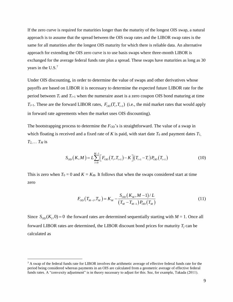
If the zero curve is required for maturities longer than the maturity of the longest OIS swap, a natural
approach is to assume that the spread between the OIS swap rates and the LIBOR swap rates is the
same for all maturities after the longest OIS maturity for which there is reliable data. An alternative
approach for extending the OIS zero curve is to use basis swaps where three-month LIBOR is
exchanged for the average federal funds rate plus a spread. These swaps have maturities as long as 30
years in the U.S.7
Under OIS discounting, in order to determine the value of swaps and other derivatives whose
payoffs are based on LIBOR it is necessary to determine the expected future LIBOR rate for the
period between Ti and Ti+1 when the numeraire asset is a zero coupon OIS bond maturing at time
Ti+1. These are the forward LIBOR rates, OD 1( , )i iF T T (i.e., the mid market rates that would apply
in forward rate agreements when the market uses OIS discounting).
The bootstrapping process to determine the FOD’s is straightforward. The value of a swap in
which floating is received and a fixed rate of K is paid, with start date T0 and payment dates T1,
T2,… TM is
1
OD OD 1 1 OD 1
0
, ,M
i i i i i
i
S K M L F T T K T T P T
(10)
This is zero when T0 = 0 and K = KM. It follows that when the swaps considered start at time
zero
OD
OD 1
1 OD
, 1 /,
M
M M M
M M M
S K M LF T T K
T T P T
(11)
Since OD 1( ,0) 0S K the forward rates are determined sequentially starting with M = 1. Once all
forward LIBOR rates are determined, the LIBOR discount bond prices for maturity Tj can be
calculated as
7 A swap of the federal funds rate for LIBOR involves the arithmetic average of effective federal funds rate for the
period being considered whereas payments in an OIS are calculated from a geometric average of effective federal
funds rates. A “convexity adjustment” is in theory necessary to adjust for this. See, for example, Takada (2011).
10
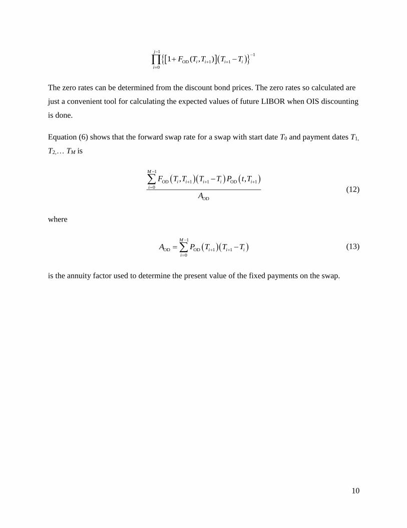
1
1
OD 1 1
0
1 ( , )j
i i i i
i
F T T T T
The zero rates can be determined from the discount bond prices. The zero rates so calculated are
just a convenient tool for calculating the expected values of future LIBOR when OIS discounting
is done.
Equation (6) shows that the forward swap rate for a swap with start date T0 and payment dates T1,
T2,… TM is
1
OD 1 1 OD 1
0
OD
, ,M
i i i i i
i
F T T T T P t T
A
(12)
where
1
OD OD 1 1
0
M
i i i
i
A P T T T
(13)
is the annuity factor used to determine the present value of the fixed payments on the swap.
11
2. OIS Discounting and LIBOR Rates
To explore how LIBOR zero rates change when OIS discounting is used, we consider the case in
which the zero curve is bootstrapped from swap market data for semi-annual pay swaps with
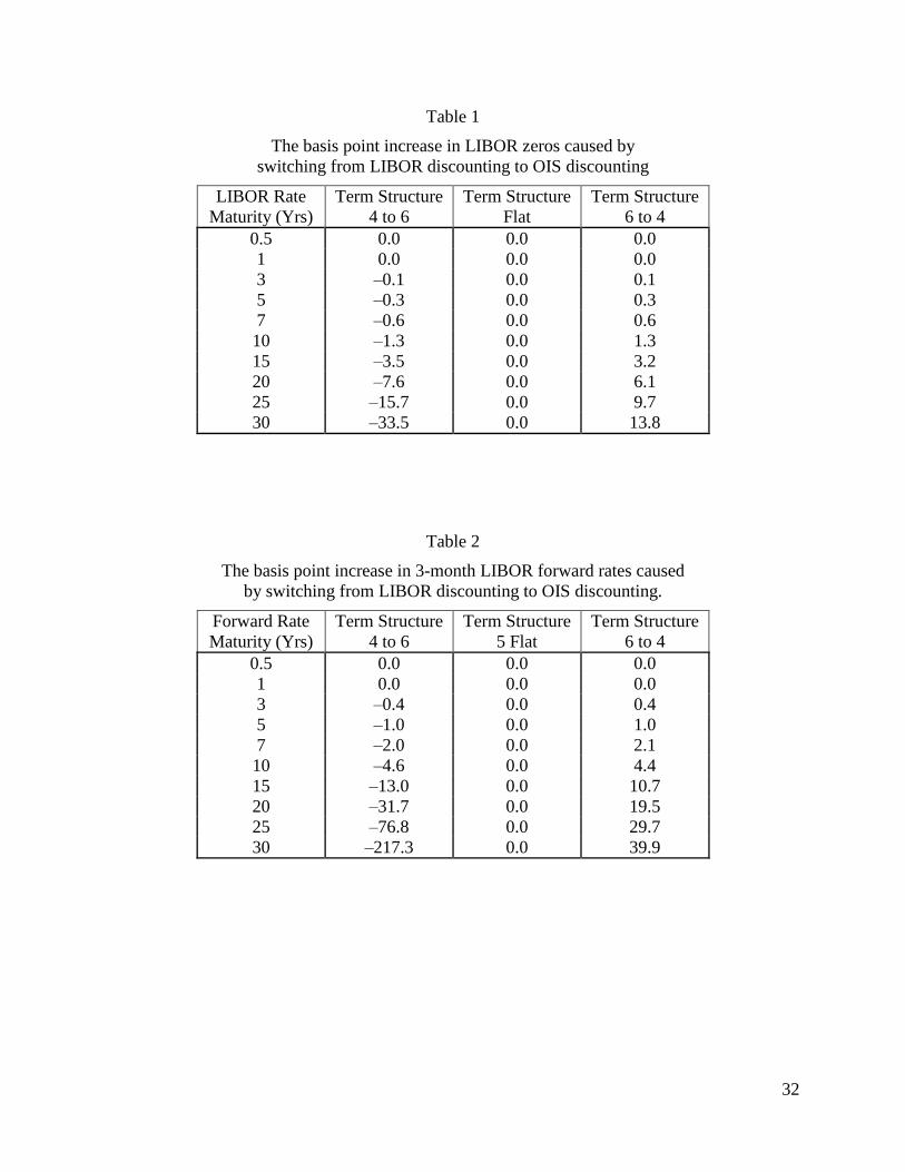
maturities from 6 months to 30 years using the procedures outlined in the previous section. Three
different sets of LIBOR swap rates are considered:
1. 4 to 6: The swap rate is 4% + 2% × Swap Life / 30.
2. 5 Flat: The swap rate is 5% for all maturities.
3. 6 to 4: The swap rate is 6% – 2% × Swap Life / 30.
We assume that the OIS swap rates equal the LIBOR swap rates less 100 basis points. (We tried
other spreads between the OIS and LIBOR swap rates and found that results are roughly
proportional to the spread.)
Table 1 shows how much the LIBOR zero curve is shifted when we switch from LIBOR
discounting to OIS discounting for the three term structures of swap rates. In an upward sloping
term structure, changing to OIS discounting lowers the value of the calculated LIBOR zero rates.
In a downward sloping term structure, the reverse is true. For a flat term structure the discount
rate used has no effect on the zero rates calculated from swap rates. This last point can be seen
by inspecting equation (4) which determines the swap value. In a flat term structure, all the
forward rates are the same so that we obtain a zero swap value if K equals the common forward
rate. This is true regardless of the level of interest rates.
For short maturities the determination of the LIBOR zero curve is not very sensitive to the
discount rate used. However, for maturities beyond 10 years, the impact of the switch from
LIBOR discounting to OIS discounting can be quite large. The impact on forward rates is even
larger. Table 2 shows 3-month LIBOR forward rates calculated using OIS discounting minus the
same three-month forward rate calculated using OIS discounting.
12
3. OIS Discounting and Swap Pricing
Changing from LIBOR discounting to OIS discounting changes the values of LIBOR swaps. In
the case of spot start swaps the value change can be expressed directly in terms of changes in the
discount factors. First, consider the swap value under LIBOR discounting. Since the value of the
floating side of an at-the-money spot start swap equals the value of the fixed side, the value of a
spot start swap in which fixed is paid can be written as
LD LD, MS K M LA K K
Similarly, when OIS discounting, is used the value becomes
OD OD, MS K M LA K K
Note that, because the calibration process ensures that at-the-money spot start swaps are
correctly priced, KM is the same in both equations. As a result the price difference is
OD LD OD LD, , MS K M S K M L K K A A
Because OIS discount rates are lower than LIBOR discount rates the last term in this expression
is positive so that, if the fixed rate being paid is below the market rate, the price change when
OIS discounting is used is positive. If the fixed rate being paid is above the market rate, the price
change is negative. For swaps where fixed is received, the reverse is true.
In general, this sort of simple decomposition of the value change is not possible. Two factors
contribute to the value change: changes in the forward rates and changes in the discount factors
used in the swap valuation. For all the interest rate derivatives we will consider in the rest of this
paper, we define
LDV : Value of derivative assuming LIBOR discounting
ODV : Value of derivative assuming OIS discounting
13
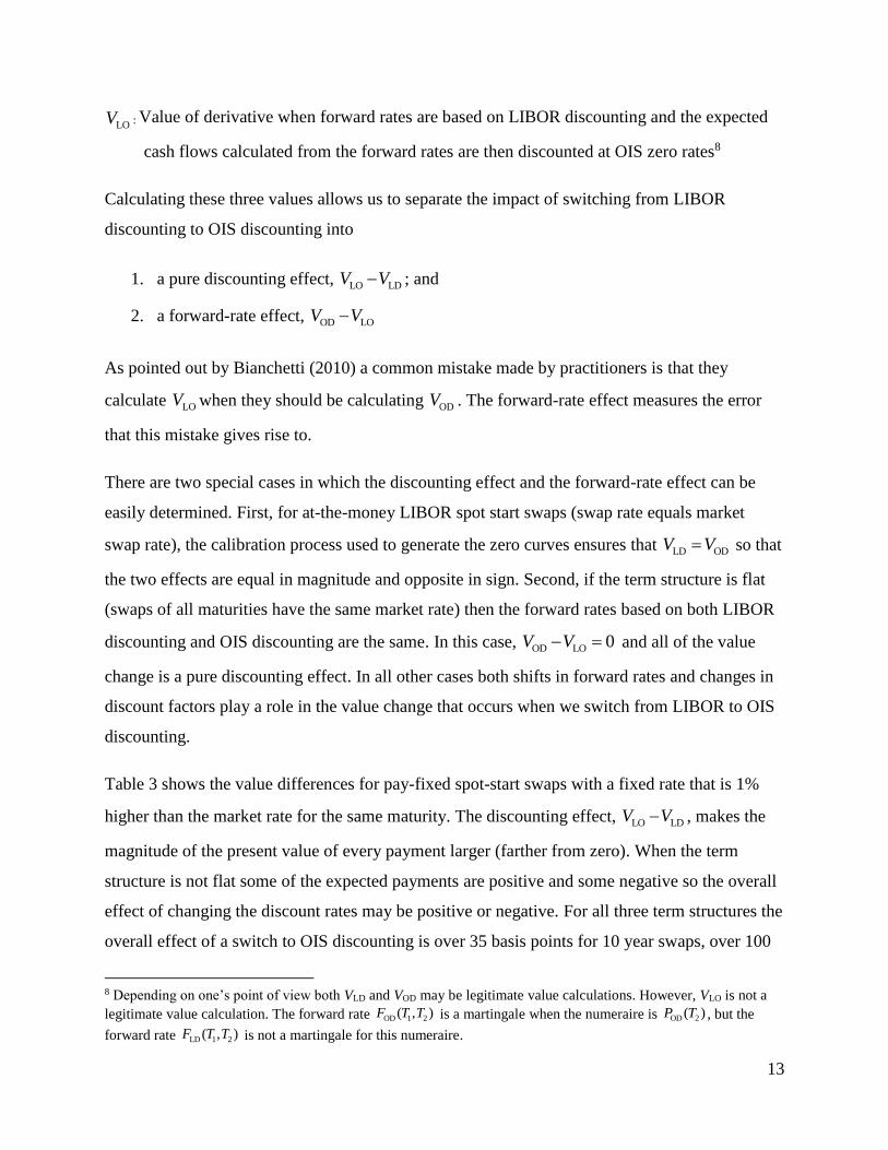
LOV : Value of derivative when forward rates are based on LIBOR discounting and the expected
cash flows calculated from the forward rates are then discounted at OIS zero rates8
Calculating these three values allows us to separate the impact of switching from LIBOR
discounting to OIS discounting into
1. a pure discounting effect, LO LDV V ; and
2. a forward-rate effect, OD LOV V
As pointed out by Bianchetti (2010) a common mistake made by practitioners is that they
calculate LOV when they should be calculating ODV . The forward-rate effect measures the error
that this mistake gives rise to.
There are two special cases in which the discounting effect and the forward-rate effect can be
swap rate), the calibration process used to generate the zero curves ensures that LD ODV V so that
the two effects are equal in magnitude and opposite in sign. Second, if the term structure is flat
(swaps of all maturities have the same market rate) then the forward rates based on both LIBOR
discounting and OIS discounting are the same. In this case, OD LO 0V V and all of the value
change is a pure discounting effect. In all other cases both shifts in forward rates and changes in
discount factors play a role in the value change that occurs when we switch from LIBOR to OIS
discounting.
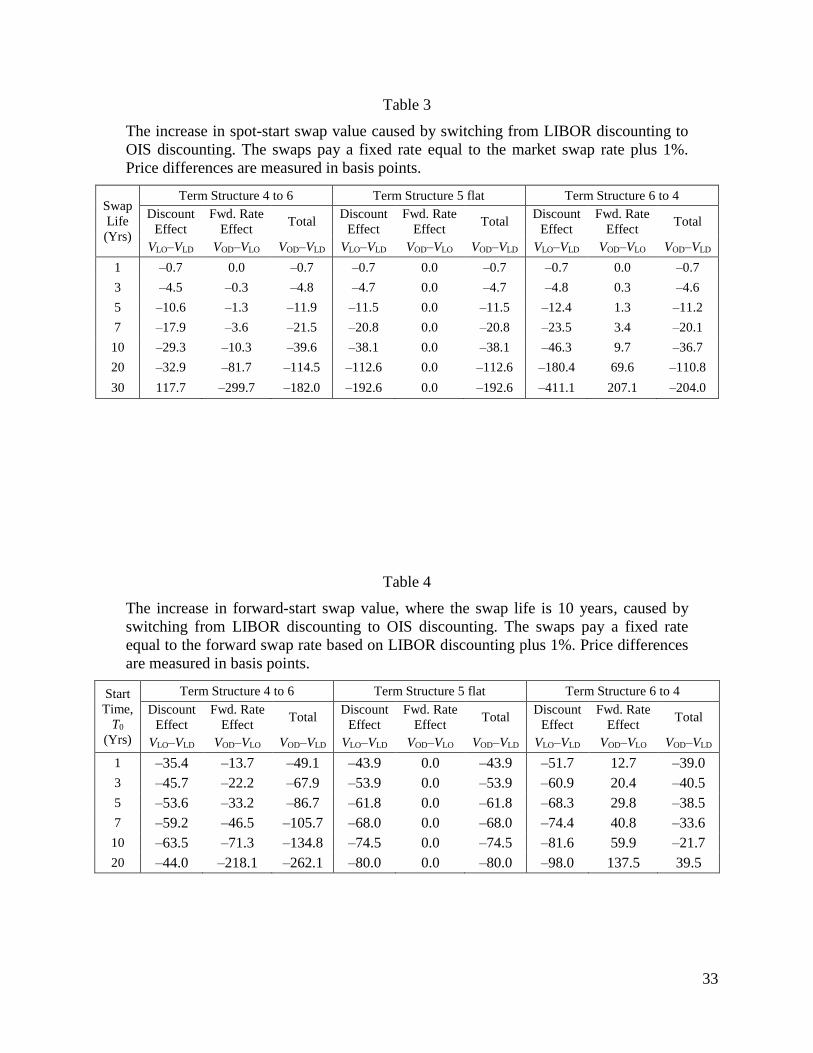
Table 3 shows the value differences for pay-fixed spot-start swaps with a fixed rate that is 1%
higher than the market rate for the same maturity. The discounting effect, LO LDV V , makes the
magnitude of the present value of every payment larger (farther from zero). When the term
structure is not flat some of the expected payments are positive and some negative so the overall
effect of changing the discount rates may be positive or negative. For all three term structures the
overall effect of a switch to OIS discounting is over 35 basis points for 10 year swaps, over 100
8 Depending on one’s point of view both VLD and VOD may be legitimate value calculations. However, VLO is not a
legitimate value calculation. The forward rate OD 1 2( , )F T T is a martingale when the numeraire is )( 2OD TP , but the
forward rate LD 1 2( , )F T T is not a martingale for this numeraire.
14
basis points for 20 year swaps, and about 200 basis points for 30 year swaps. The table shows
that for non-flat term structures, the forward rate effect can be quite large and calculating
forward rates using the pre-crisis approach can therefore lead to large errors. Indeed, for the
upward sloping term structure we consider, the forward rate effect is bigger than the pure
discounting effect when the swap lasts 20 or 30 years.
Table 4 shows the value differences for forward start swaps where the swap life is 10 years. The
fixed rate is paid and LIBOR is received. The fixed rate is 1% higher than the corresponding
forward swap rate based on LIBOR discounting. Again, for upward and downward sloping term
structures and long maturities, the impact of using the wrong forward rates in conjunction with
OIS discounting can lead to large errors.
15
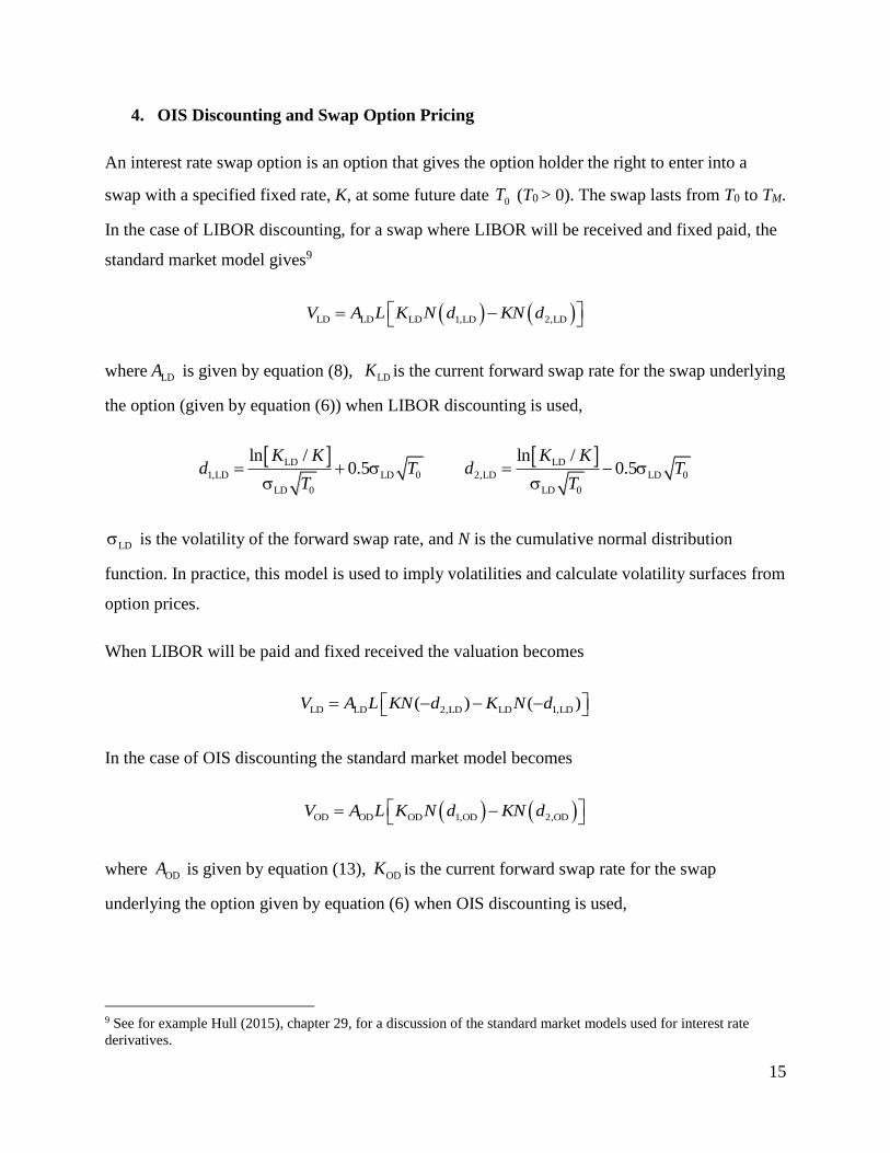
4. OIS Discounting and Swap Option Pricing
An interest rate swap option is an option that gives the option holder the right to enter into a
swap with a specified fixed rate, K, at some future date 0T (T0 > 0). The swap lasts from T0 to TM.
In the case of LIBOR discounting, for a swap where LIBOR will be received and fixed paid, the
standard market model gives9
LD LD LD 1,LD 2,LDV A L K N d KN d
where LDA is given by equation (8), LDK is the current forward swap rate for the swap underlying
the option (given by equation (6)) when LIBOR discounting is used,
LD LD
1,LD LD 0 2,LD LD 0
LD 0 LD 0
ln / ln /0.5 0.5
K K K Kd T d T
T T
LD is the volatility of the forward swap rate, and N is the cumulative normal distribution
function. In practice, this model is used to imply volatilities and calculate volatility surfaces from
option prices.
When LIBOR will be paid and fixed received the valuation becomes
LD LD 2,LD LD 1,LD( ) ( )V A L KN d K N d
In the case of OIS discounting the standard market model becomes
OD OD OD 1,OD 2,ODV A L K N d KN d
where ODA is given by equation (13), ODK is the current forward swap rate for the swap
underlying the option given by equation (6) when OIS discounting is used,
9 See for example Hull (2015), chapter 29, for a discussion of the standard market models used for interest rate
derivatives.
16
OD OD
1,OD OD 0 2,OD OD 0
OD 0 OD 0
ln / ln /0.5 0.5
K K K Kd T d T
T T
and OD is the volatility of the forward swap rate.10 When LIBOR will be paid and fixed
received, the OIS-discounting valuation becomes
OD OD 2,OD OD 1,OD( ) ( )V A L KN d K N d
This version of the standard market model, like the original version given above, can be used to
imply volatilities and calculate volatility surfaces from option prices.
To examine the effect of the switch to OIS discounting on the prices of swap options we consider
options with lives between 1 and 20 years on a 5-year swap when the volatility for all maturities
is set equal to 20% for both LIBOR and OIS discounting. In every case the option strike price, K,
is set equal to LDK . For the LIBOR discounting case, the options are exactly at-the-money while
in the OIS discounting case the options are approximately at-the-money.
Table 5 shows the value differences for options to enter into swaps in which floating is paid for
the three terms structures of swap rates. Table 6 shows similar results for options to enter into
swaps in which fixed is paid. The effect of changing the discount factors is about the same for
both pay fixed and pay floating swaps. However, changing forward rates has a much more
pronounced effect on the value of options on swaps in which the option holder pays the fixed
rate. This is because pay-fixed (pay-floating) swap options provide payoffs when swap rates are
high (low). The forward swap rate is assumed to follow geometric Brownian motion and so a
change in the starting forward swap rate has a greater effect on high swap rates than on low swap
rates.
In practice option pricing models are calibrated to market prices by implying volatilities. This
has implications for the implied volatility surface calculated by a dealer for whom discounting
practices are not in alignment with market practice. Consider the case of Dealer X who is the
first dealer to consider switching from LIBOR to OIS discounting for option pricing purposes.
10 Note that OD and LD are in general not equal.
17
Since all other dealers are using LIBOR discounting observed market prices for swap options are
given by VLD. When Dealer X calibrates his swap option pricing model to the observed market
prices, the price differences caused by the different approaches to discounting translate into
differences in the implied volatility.
To illustrate this, we calculate option prices for options with lives from 1 to 20 years on a five
year swap based on LIBOR discounting, VLD. The fixed rate on the swap is the forward swap rate
based on LIBOR discounting plus an offset of between –2% and +2%. The volatility of the
forward swap rate is 20% for all strikes and maturities. These prices are then backed through the
OIS discounting swap option pricing model to find the implied volatility that set VOD = VLD.
The results depend on the slope of the term structure and the terms of the options. Figure 1
shows the volatility term structure that Dealer X would calculate for options to enter into a swap
that pays fixed that when term structure of interest rates is upward sloping. The implied
volatilities are always less than the market volatility used in the LIBOR discounting option
pricing model. The volatility term structure is generally downward sloping except for in-of-the
money options which exhibit a steeply upward sloping term structure for relatively short-term
options.
Figure 2 shows the shape of the volatility smile for the same set of options. The implied
volatilities are highest for out-of-the-money options and lowest for in-the-money options. The
smile is most pronounced for short maturity options and becomes increasingly flatter as the
option maturity lengthens. For at- and out-of-the-money options longer term options have lower
implied volatilities. The reverse is true for deep in-the-money options.
A similar situation applies to a Dealer Y who uses LIBOR discounting when the observed
market prices for swap options are given by VOD. When Dealer Y calibrates his swap option
pricing model to market prices he will in a similar way observe a volatility surface resulting from
the different pricing characteristics of the two option pricing models.
Because both OIS discounting and LIBOR discounting models are calibrated to market data the
main effect of the differences in the models will in practice be captured by the implied
18
volatilities. As a result the models will agree perfectly for all options in the calibration set and
the price differences for other options will be small.
19
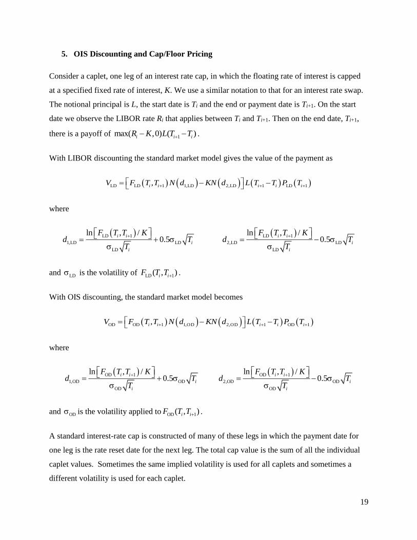
5. OIS Discounting and Cap/Floor Pricing
Consider a caplet, one leg of an interest rate cap, in which the floating rate of interest is capped
at a specified fixed rate of interest, K. We use a similar notation to that for an interest rate swap.
The notional principal is L, the start date is Ti and the end or payment date is Ti+1. On the start
date we observe the LIBOR rate Ri that applies between Ti and Ti+1. Then on the end date, Ti+1,
there is a payoff of 1max( ,0) ( )i i iR K L T T .
With LIBOR discounting the standard market model gives the value of the payment as
LD LD 1 1,LD 2,LD 1 LD 1,i i i i iV F T T N d KN d L T T P T
where
LD 1 LD 1
1,LD LD 2,LD LD
LD LD
ln , / ln , /0.5 0.5
i i i i
i i
i i
F T T K F T T Kd T d T
T T
and LD is the volatility of LD 1( , )i iF T T .
With OIS discounting, the standard market model becomes
OD OD 1 1,OD 2,OD 1 OD 1,i i i i iV F T T N d KN d L T T P T
where
OD 1 OD 1
1,OD OD 2,OD OD
OD OD
ln , / ln , /0.5 0.5
i i i i
i i
i i
F T T K F T T Kd T d T
T T
and OD is the volatility applied to ),( 1OD ii TTF .
A standard interest-rate cap is constructed of many of these legs in which the payment date for
one leg is the rate reset date for the next leg. The total cap value is the sum of all the individual
caplet values. Sometimes the same implied volatility is used for all caplets and sometimes a
different volatility is used for each caplet.
20
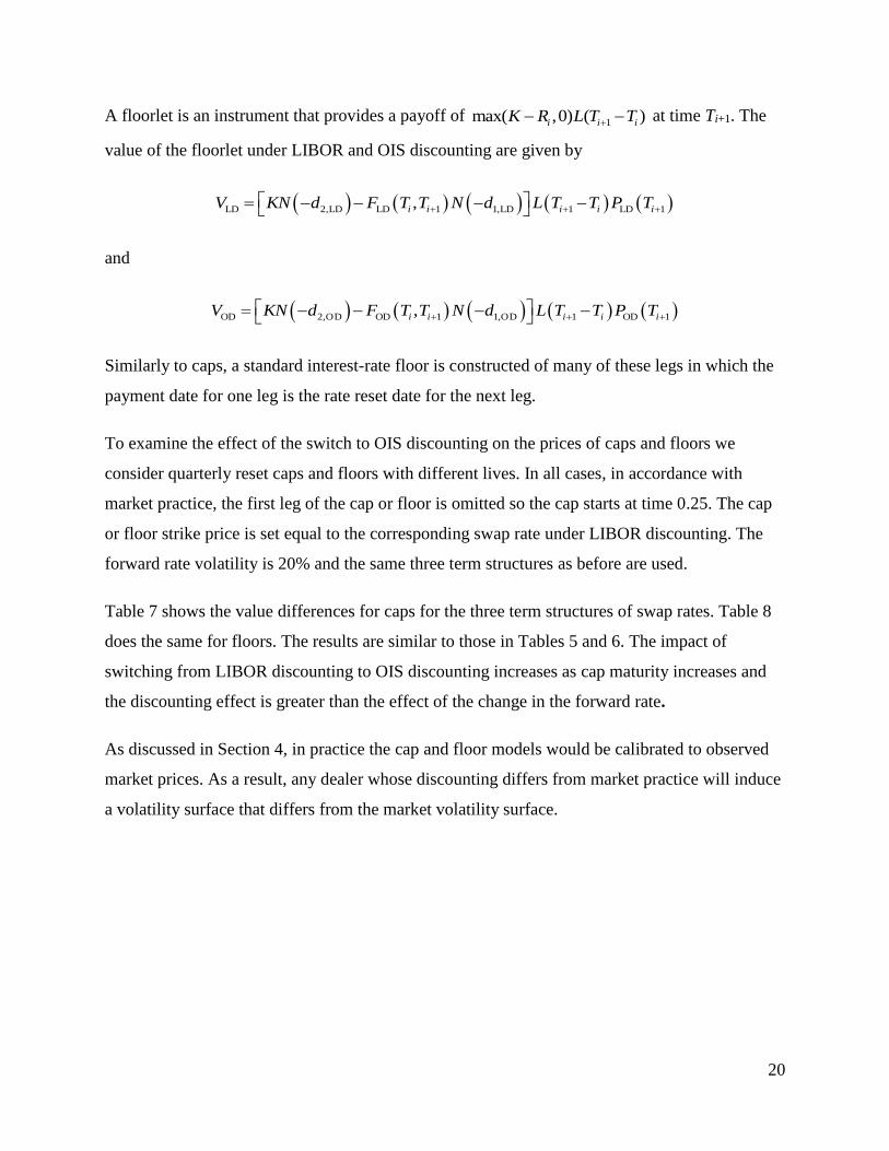
A floorlet is an instrument that provides a payoff of 1max( ,0) ( )i i iK R L T T at time Ti+1. The
value of the floorlet under LIBOR and OIS discounting are given by
LD 2,LD LD 1 1,LD 1 LD 1,i i i i iV KN d F T T N d L T T P T
and
OD 2,OD OD 1 1,OD 1 OD 1,i i i i iV KN d F T T N d L T T P T
Similarly to caps, a standard interest-rate floor is constructed of many of these legs in which the
payment date for one leg is the rate reset date for the next leg.
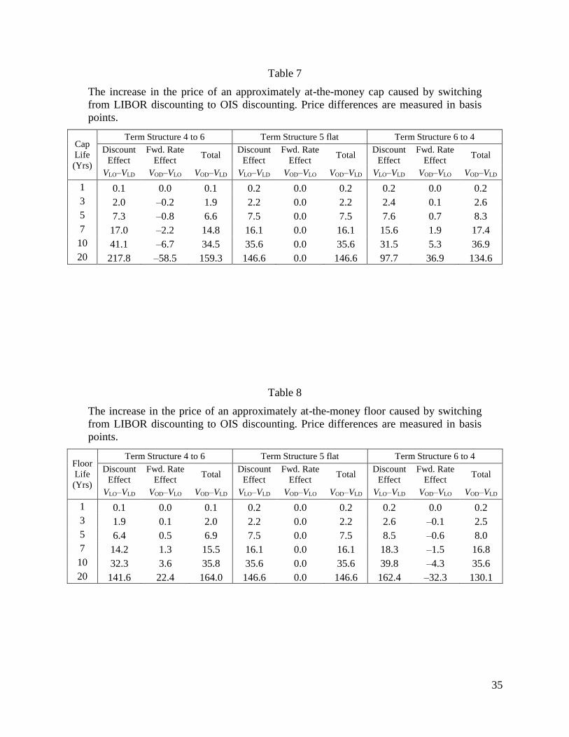
To examine the effect of the switch to OIS discounting on the prices of caps and floors we
consider quarterly reset caps and floors with different lives. In all cases, in accordance with
market practice, the first leg of the cap or floor is omitted so the cap starts at time 0.25. The cap
or floor strike price is set equal to the corresponding swap rate under LIBOR discounting. The
forward rate volatility is 20% and the same three term structures as before are used.
Table 7 shows the value differences for caps for the three term structures of swap rates. Table 8
does the same for floors. The results are similar to those in Tables 5 and 6. The impact of
switching from LIBOR discounting to OIS discounting increases as cap maturity increases and
the discounting effect is greater than the effect of the change in the forward rate.
As discussed in Section 4, in practice the cap and floor models would be calibrated to observed
market prices. As a result, any dealer whose discounting differs from market practice will induce
a volatility surface that differs from the market volatility surface.
21
6. Building Trees to Value Nonstandard Transactions
So far this paper has focused on transactions which are handled by the market using standard
market models based on Black (1986). As we have shown, it is fortunate that, once forward
LIBOR has been correctly calculated, only a small modification to the standard market models is
necessary.11 We now move on to consider instruments which cannot be handled using standard
market models. A single interest rate tree describing the evolution of the LIBOR rates is
commonly used to value these instruments when LIBOR discounting is used. In this section, we
explain that it is still possible to obtain a value using a single tree when OIS discounting is used.
For the sake of definiteness, consider a derivative providing payoffs dependent on three-month
LIBOR.12 The general procedure is as follows:
1. Calculate the OIS zero curve from swap rates as discussed earlier in this paper.
2. Calculate a LIBOR zero curve when OIS discounting is used as discussed earlier in this
paper.
3. Assume a one-factor interest rate model for the evolution of the OIS zero curve and
construct a tree for the t-period OIS rate. The drift of the short rate will typically include
a function of time so that the initial OIS term structure is matched. Procedures for
building the tree are described in, for example, Hull and White (1994) and Hull and
White (2014).
4. Roll back through the tree to calculate the value of a three-month bond at each node so
that the three-month OIS rate is known at each node.
5. Assume a one-factor model for the spread between the three-month LIBOR rate and the
three-month OIS rate. Similarly to the model for the OIS rate, this will include a function
of time so that the LIBOR zero curve can be matched.
11 As an alternative to using standard market models, one can value caplets or swap options by integrating over the
joint distribution of OIS and the spread. This approach is discussed by Mercurio and Xie (2012) 12 The same approach can be used for derivatives dependent on any other reference rate. If the tenor of the reference
is a single tree is use to model the OIS t -period rate and the expected spread between the -period OIS rate and
the -period reference rate.
22
6. Assume a correlation between the three-month OIS rate and the spread in step 5.
7. Advance through the OIS tree one step at a time matching the tree-based value of a
forward rate agreement based on three-month LIBOR rates with the analytic value
calculated using the procedures described in Section 3. The procedure is as follows: At
the time t step choose a trial value for the unconditional expected spread at time t. (As
mentioned, the process for the spread incorporates a function of time in the drift.)
Calculate the conditional expected spread at each node of the OIS tree at time t based on
the unconditional expected spread. The expected three-month LIBOR rate at each node of
the OIS tree is then the three-month OIS rate at the node plus the expected spread. The
value of the forward rate agreement at each node at time t can be calculated from the 3-
month LIBOR and OIS rates at the node. Discounting these values back through the tree
produces the tree-based estimate of the value of the forward rate agreement. (These
present value calculations are simplified by storing the Arrow-Debreu prices at each node
when the OIS tree is constructed in step 3.) An iterative procedure is used to determine
the unconditional expected spread at time t that matches the tree-based price with the
analytic price.
The result of this procedure is a tree that has the OIS rate and the expected LIBOR rate at each
node. The tree matches both the OIS swap rates and LIBOR swap rates. It can be used to value
derivatives whose payoffs depend on LIBOR when OIS discounting is used.
The potentially difficult part of the procedure is calculating the expected spread at time t at each
node of the OIS tree for a trial value of the unconditional expected spread at time t. For some
models analytic results are available. In other cases numerical procedures can be developed.13
The appendix shows that analytic results are available when a) a mean-reverting Gaussian model
is used for both the instantaneous OIS rate and the spread and b) a mean-reverting Gaussian
model is used for both the logarithm of the OIS rate and the logarithm of the spread. The first
13 A general numerical procedure that can be used is as follows. Construct a tree for the t-OIS rate, r. Construct a
tree step-by-step for the spread, s. At the each time step, determine the unconditional distributions for r and s. (In the
case of the s-tree a trial value for the center of the tree is being assumed.) Assume a Gaussian copula (or some other
convenient copula) to determine rsE at each node of the r-tree. The advantage of the analytic results given in
the appendix for the normal and the lognormal models is that calculations are much faster because it is not necessary
to build the s-tree.
23
model can be viewed as a natural extension of Hull and White (1990) interest rate model. The
second can be viewed as a natural extension of Black and Karasinski (1991) interest rate model.
When valuing American-style options, there is the complication that the decision to exercise at a
node may depend on the value of the spread, s, at the node. This can be accommodated as
follows. First we calculate for the node the critical value of s above which early exercise is
optimal. We will refer to this as s*. Define Rssq Pr . The value of the option at the node
is
21)1( qUUq
where 1U is the value of the option (calculated from the value at subsequent nodes) if there no
exercise and 2U is the intrinsic value of the option at the node. The calculation of q is explained
in the appendix for the two models considered.
We will illustrate the model using the extension of Black and Karasinski (1991). Specifically, if r
is the short term OIS rate and x=ln(r), then
xxx dzdtxatdx )(
where ax and x are positive constants, (t) is a function of time chosen to match the OIS zero
curve that is calculated from OIS swap rates, and dzx is a Wiener process. If s is the three-month
LIBOR−OIS spread and y = ln(s)
( ) y y ydy t a y dt dz
where ay and y are positive constants, (t) is a function of time, and dzy is a Wiener process.
The correlation between dzx and dzy is assumed to be a constant, .
We consider a ten-year Bermudan swap option where early exercise can take place on each swap
payment date on or after year two. The holder has an option to enter into the swap. The swap
underlying the option is a quarterly reset swap in which 3-month LIBOR is received and a fixed
rate is paid. The fixed rate is set equal to the market rate for a swap that starts in two years and
24
matures in ten years. This ensures that at the first possible exercise date, two years from now, the
option is approximately at the money. The OIS and LIBOR term structure data is the same as
that for the first of the three cases defined in Section 2. The instantaneous OIS rate volatility, x,
is 20%, the reversion rate, ax, is 5%, and the LIBOR-OIS spread reversion rate, ay, is 5%. We
consider a number of different values of y and .
A necessarily prerequisite to valuing the Bermudan swap option is valuing the underlying swap
at each node of the tree. This can be calculated by rolling back through the tree in the usual way.
The value of the swap at a node at time it is the present value of the expected value at the nodes
that can be reached at time (i+1)t plus the present value of any payment based on the expected
value of LIBOR at the node.
The value of the option for various values of the LIBOR−OIS spread volatility, y, and the
correlation, , between the spread and the OIS rate are shown in Table 9. The value of the option
when the spread is constant, y = 0, is 2.92% of the swap notional. If the correlation is positive
the option value increases as the spread volatility increases while if the correlation is negative the
option value decreases as the spread volatility increases. The reason for this is that when the OIS
rate is high and the correlation is positive the LIBOR−OIS spread is greater than average.
Similarly, when the OIS rate is low and the correlation is positive the LIBOR−OIS spread is
smaller than average. As a result, the LIBOR rate (i.e., the OIS rate plus the spread) exhibits
more variability than the OIS rate. This increases the value of options on the LIBOR rate. If the
correlation is negative the reverse is true and the LIBOR rate exhibits less variability than the
OIS rate resulting in lower option prices.
The results show that a correlation between the spread and OIS can have an appreciable effect on
option prices. For example, when the spread volatility is 15% and the correlation is 0.25 the
value of the option increases by about 5%. This result is predicated on the assumption that we
know the volatility of OIS and the spread. However, in practice all model parameters are
typically implied from the observed market prices for options with different strike prices and
times to maturity. The model is in effect a tool for pricing non-standard interest rate derivatives
consistently with standard interest rate derivatives. As a result, the calibrated OIS and spread
25
volatility parameters will be sensitive to the assumed correlation but option prices calculated
using the calibrated models will be much less sensitive to this correlation.
26
7. Conclusions
When interest rate derivatives are valued, moving from LIBOR to OIS discounting has two
effects. First, forward interest rates and forward swap rates change. Second, the discount rates
applied to the cash flows calculated from those forward rates change. The impact of the switch is
small for short-dated instruments but becomes progressively larger as the life of the instrument
becomes longer.
One mistake that is sometimes made is to a) calculate LIBOR zero rates and LIBOR forward
rates and by bootstrapping LIBOR forward swap rates in the traditional way (i.e., in a world
where LIBOR discounting is employed) and b) apply OIS discount rates to the cash flows
calculated by assuming that the LIBOR forward rates will be realized. Our results show the
errors caused by making this mistake. The error is zero for flat term structures, but can be as
much as 200 basis points for long-dated transactions and the upward or downward sloping term
structures we have considered.
This paper has shown how the standard market models for caps and swap options can be adjusted
to accommodate OIS discounting. For more complex instruments we have presented a new
procedure for adjusting the way interest rate trees are used to accommodate OIS discounting.
Both the OIS rate and the expected LIBOR rate can be modeled using a single tree. A stochastic
spread makes LIBOR more (less) volatile than OIS if the correlation is positive (negative). This
results in higher (lower) option prices than arise when the spread is deterministic.
27
References
Bianchetti, Marco (2010), “Two Curves, One Price,” Risk, 23, 8 (August): 66-72.
Black, Fischer (1976), “The pricing of Commodity Contracts,” Journal of Financial Economics, 3
(March): 167-179.
Black, Fischer and Piotr Karasinski (1991), "Bond and Option Pricing When Short Rates Are