Old, Sick, Alone and Poor: A Welfare Analysis of Old-Age Social Insurance Programs * R. Anton Braun Federal Reserve Bank of Atlanta [email protected]Karen A. Kopecky Federal Reserve Bank of Atlanta [email protected]Tatyana Koreshkova Concordia University and CIREQ [email protected]May 2013 Abstract Poor heath, large acute and long-term care medical expenses and spousal death are significant drivers of impoverishment among retirees. We document these facts and build a rich overlapping generations model that reproduces them. We use the model to assess the incentive and welfare effects of U.S. Social Security and means-tested social insurance programs, such as Medicaid and food stamp programs, for the aged. We find that U.S. means-tested social insurance programs for retirees provide significant welfare benefits for all newborn. Moreover, when means-tested social insurance benefits are of the scale in the U.S., all newborn prefer that Social Security be removed. Finally, we find that the current scale of means-tested social insurance in the U.S. is about right in the following sense. If we condition on the current Social Security program, the benefits of increasing means-tested social insurance are small or negative. Keywords: Social Security; Medicaid; Social Insurance; Elderly; Medical Expenses. JEL Classification numbers: E62, H31, H52, H55. * We thank Mark Bils, Erich French, Victor R´ ıos and Gianluca Violante for their helpful comments and Neil Desai for excellent research assistance. We thank seminar participants at the Federal Reserve Bank of Atlanta. We are also grateful for comments from conference participants at the Wegman’s Conference at the University of Rochester 2010, the 2012 Conference on Health and the Macroeconomy at the Laboratory for Aggregate Economics and Finance, UCSB, Fall 2012 Midwest Macroeconomics Meetings, 2013 MRRC Workshop, 2013 QSPS Summer Workshop, 2013 CIGS Conference on Macroeconomic Theory and Policy and the 2013 SED Meetings. 1
Poor heath, large acute and long-term care medical expenses and spousal death are
significant drivers of impoverishment among retirees. We document these facts and
build a rich overlapping generations model that reproduces them. We use the model to
assess the incentive and welfare effects of U.S. Social Security and means-tested social
insurance programs, such as Medicaid and food stamp programs, for the aged. We find
that U.S. means-tested social insurance programs for retirees provide significant welfare
benefits for all newborn. Moreover, when means-tested social insurance benefits are of
the scale in the U.S., all newborn prefer that Social Security be removed. Finally, we
find that the current scale of means-tested social insurance in the U.S. is about right
in the following sense. If we condition on the current Social Security program, the
benefits of increasing means-tested social insurance are small or negative.
Keywords: Social Security; Medicaid; Social Insurance; Elderly; Medical Expenses.
JEL Classification numbers: E62, H31, H52, H55.
∗We thank Mark Bils, Erich French, Victor Rıos and Gianluca Violante for their helpful comments andNeil Desai for excellent research assistance. We thank seminar participants at the Federal Reserve Bank ofAtlanta. We are also grateful for comments from conference participants at the Wegman’s Conference atthe University of Rochester 2010, the 2012 Conference on Health and the Macroeconomy at the Laboratoryfor Aggregate Economics and Finance, UCSB, Fall 2012 Midwest Macroeconomics Meetings, 2013 MRRCWorkshop, 2013 QSPS Summer Workshop, 2013 CIGS Conference on Macroeconomic Theory and Policyand the 2013 SED Meetings.
All individuals face some risk of ending up old, sick, alone and poor. Those who find
themselves in this situation are often unable to work their way out of poverty by re-entering
the labor force. In the U.S. two types of social insurance (SI) help retirees cope with this
outcome: Social Security (SS) and means-tested SI such as Medicaid, Supplemental Social
Security Income, food stamps, housing and energy assistance programs.
Milton Friedman in Cohen and Friedman (1972) argued that there is no need for SS and
that a means-tested SI program is an efficient way to help retirees cope with this outcome.
Feldstein (1987) showed that SS can be better than means-tested SI and went on to suggest
that there may be a welfare enhancing role for having both programs when individuals are
heterogenous.
Our objective is to consider the welfare and incentive effects of SS and means-tested
SI programs in a model that explicitly recognizes the possibility that retirees may end up
being old, sick, alone and poor. Consistent with Friedman, we find that there is no welfare
enhancing role for SS when means-tested SI benefits are of the scale in the U.S. This result
occurs in spite of the fact that removing SS has the large, negative incentive effects on savings
of poorer households emphasized by Feldstein. This is not to say that there is no need for
public SI for the aged. We find that means-tested SI has an important welfare enhancing
role for retirees and that its current scale in the U.S. is about right. Modeling medical and
long-term care expenses plays an essential role in these results.
A large macroeconomics literature has analyzed the role of SS in settings where there
is only survival and/or lifetime earnings risk. A robust conclusion from this literature is
that a pay-as-you-go SS program is bad public policy. This result has been documented
in models with dynastic households as in Fuster, Imrohoroglu and Imrohoroglu (2007) and
also in a broad range of life cycle OLG models starting with the research of Auerbach and
Kotlikoff (1987). Imrohoroglu, Imrohoroglu and Joines (1999) show that this result holds in
dynamically efficient economies. Conesa and Krueger (1998) find that this result holds when
agents face life-time earnings risk. Rıos and Hong (2007) show that this result holds when
the economy is open and the pre-tax real interest rate is fixed. They also show that the result
does not depend on the availability of private market substitutes such as private annuities
and private life insurance. One exception to this general finding is Nishiyama and Smetters
(2007) who show that the transition costs of privatizing SS may exceed the long-term benefits
associated with a smaller SS program when labor market risk is uninsured.
A second and smaller strand of the literature has analyzed the efficacy of means-tested
2
SI for retirees who are subject to permanent-earnings and survival risk.1 The idea that a
means-tested SI program is more efficient than a universal SS program dates back to a debate
by Wilbur Cohen and Milton Friedman. Friedman argued that the negative incentive effects
of universal SS were so large that welfare would be improved if SS was replaced with a means-
tested SI program (see Cohen and Friedman, 1972). In subsequent work, Feldstein (1987)
has argued that means-tested SI for retirees has a particularly strong, negative incentive
effect on some individuals. When means-tested SI is available and sufficiently liberal, these
individuals will choose to consume all of their income when young and to rely on means-tested
SI when they retire.
Tran and Woodland (2012) perform a quantitative general equilibrium analysis of Aus-
tralia’s public pension system. Australia is interesting because all public pensions are means-
tested. They compare Australia’s current system with an alternative economy with no
means-tested public pension and find that agents prefer to be born into the latter economy.
In their model the negative incentive effects emphasized by Feldstein (1987) are so strong
that they dominate the positive insurance effects of means-tested SI. However, means-tested
public pensions can be welfare improving if means-tested benefits are tapered off in a suitable
way.
Perhaps the most relevant analysis to our question is conducted by Sefton, van de Ven
and Weale (2008) who compare a universal SS system with the UK means-tested programs:
the Minimum Income Guarantee program was in place prior to 2003 and narrowly targeted
the poor; and the post-2003 UK public pension plan which lowered the effective tax rate
on benefits from 100 to 40% of private income. They find in favor of Friedman. Young
individuals prefer either form of means-tested public pension system over a universal SS
system when factor prices are allowed to adjust and the fiscal budget is balanced.
This previous literature focuses exclusively on survival and permanent earnings risks
and abstracts, in all cases, from medical and long-term care expense risk. Imrohoroglu,
Imrohoroglu and Joines (1995) do model catastrophic health risk and find that modeling
medical expenses does not have a large effect on savings and the welfare implications of
SS reform. Their calibration of medical expenses is based on estimates by Feenberg and
Skinner (1991). French and Jones (2004) have shown that Feenberg and Skinner (1991)
underestimate the extent of medical expense risk faced by the elderly. DeNardi, French
and Jones (2010) estimate a structural model of medical expenses faced by retirees and
find that these expenses influence savings decisions of both rich and poor retirees. Kopecky
and Koreshkova (2007) show that old-age, long-term care expenses and their risk have a
1Means-tested support for working individuals has received more attention in the literature, see e.g.Hubbard, Skinner and Zeldes (1995).
3
significant effect on aggregate savings.
Medical and long-term care expenses are important risk factors for retirees because they
increase with age and are concentrated in the final periods of life. These expenses are also
correlated with other life events. For instance, a spousal death event that is preceded by
large nursing home or hospital expenses can impoverish the survivor. We start by providing
new evidence that widowhood, poor health, and hospital and nursing home stays are all
associated with higher transitions into poverty. We then model these old age risks in a
general equilibrium, life-cycle model of the U.S. economy.
Individuals enter the economy with a given level of educational attainment and a spouse
and stay married throughout their working life. Labor productivity of working-age house-
holds evolves stochastically over the life-cycle and a borrowing constraint limits their ability
to self-insure. Men’s labor is supplied to the market inelastically, while female’s labor supply
is optimally chosen by the household. At age 65, all individuals retire.
Retired individuals in our model are subject to survival risk, health and out-of-pocket
(OOP) medical expense risk, including the risk of a lengthy nursing home stay, and spousal
death risk. These risks vary with age, gender and marital status of the retiree and are
correlated with the retiree’s education type. Thus retired households are heterogeneous
not only in the size of their accumulated wealth (private savings and pensions), but also
in the life expectancies of their members, household OOP medical expenses and household
composition. We assume that there are no markets to insure against productivity, health,
or survival risk. Partial insurance, however, is available to retirees through two programs
run by the government: a progressive pay-as-you-go SS program that includes spousal and
survivor benefits, and a means-tested SI program that guarantees a minimum consumption
level to retirees.
We calibrate the model to match a set of aggregate and distributional moments for the
U.S. economy, including demographics, earnings, medical and nursing home expenses, as
well as features of the U.S. means-tested social welfare, SS and income tax systems. We
then assess the model’s ability to reproduce key facts observed in the data but not targeted
in the calibration. In particular, we show that the model generates patterns consistent with
the data with regards to Medicaid take-up rates, flows into Medicaid and OOP medical
expenses by age and marital status. Moreover, we show that the model delivers an increased
likelihood of impoverishment for individuals who experience: large acute and long-term
care OOP expenses; shocks to health status; or a spousal death event. These patterns
of impoverishment in the model are in line with impoverishment statistics in our dataset
obtained from the Health and Retirement Survey (HRS).
To assess Friedman’s claim that means-tested SI is an efficient way to insure retirees
4
against old-age risks, we start by comparing economies with only SS or only means-tested
SI, of the scale of these programs in the U.S., with an economy with no SI. Introducing SS into
an economy with no SI programs reduces average welfare by 5.11% of lifetime consumption.
This occurs because the return on SS contributions is much lower than the effective real
return on private savings.2
We consider next compare the economy with no SI with an economy with means-tested
SI only. Consistent with Feldstein’s arguments we find that introducing means-tested SI
has a significant negative incentive effect on the poor and many chose not to save at all for
retirement. Twenty-one percent of individuals roll into means-tested SI immediately upon
retiring. However, these negative incentive effects are dominated by a positive insurance
effect and average welfare of a newborn increases by 14%. This large positive insurance
effect stems from the fact that means-tested SI transfers pay out in situations where medical
expenses are large and thus the need for insurance is greatest. SS benefits do not have this
state-contingent feature and are therefore a less effective form of insurance against old-age
medical risks.
Even though we find that SS only is not welfare improving, it could be that there is a
welfare enhancing role of having both means-tested SI and SS due to interactions between
the two programs. To ascertain the answer we consider the introduction of SS into the
economy with means-tested SI only. Introducing SS lifts a large fraction of retirees out of
poverty. Means-tested take-up rates of retirees decline from 34% to 13% and government
outlays on this program fall from 2.52% to 0.80% of GNP. The reason why introducing SS
has such a dramatic impact on means-tested SI take-up rates is because it ameliorates the
negative saving effect of means-tested SI. SS ’forces’ some households, who would choose
not to save otherwise, to save for retirement. This forced savings increases the effective
expected return from saving and some households alter their strategy and choose to save on
their own as well. This fiscal benefit of introducing SS is not welfare improving: welfare of
all types of newborn falls. Affluent households like this fiscal benefit but the poor do not.
Effectively forcing the poor to save lowers their utility. These factors in conjunction with the
low effective return of SS contributions act to lower average welfare of newborn by 11.8%.
Thus we find that even though the negative incentive effects emphasized by Feldstein are
large, Friedman’s suggestion that SS be removed enhances welfare in the long-run.
Our results suggest that there may be a role for increasing the scale of means-tested SI
in the U.S. To explore this possibility, we condition on the current SS program and consider
2This cost of SS is well known and is most pronounced when the real interest rate is held fixed. It stemsfrom the fact that the effective return on SS contributions is given by the growth rate of aggregate laborincome which is lower than the effective real return on capital in a dynamically efficient economy.
5
two strategies for financing a 30 percent increase in means-tested SI benefits for retirees.
When the increase is financed by a payroll tax, welfare increases by 0.54% of consumption.
However, when the increase is financed by income taxes, welfare falls instead by -0.44%.
Medical and long-term care expenses play a central role in our findings. When medical
expenses are set to zero, households prefer an economy with no SI instead of our represen-
tation of the U.S. economy with both SI programs. Medical expense risks also matter for
the size of the disincentive effects emphasized by Feldstein (1987). These negative incentive
effects become very small when medical expenses are zero. Finally, medical expense risks
affect the welfare benefits of means-tested SI. The benefits provided by this program are
much more valuable to households when medical expense risks are present.
The remainder of the paper is organized as follows. In Section 2, we motivate our analysis
by providing evidence on sources of impoverishment for the elderly. Section 3 describes the
model. Section 4 reports how we estimate and calibrate the various parameters and profiles
that are needed to solve the model. In Section 5, we assess the ability of the model to
reproduce statistics not targeted in the calibration, including flows into Medicaid by age and
martial status, as well as a variety of wealth mobility statistics for retirees. Section 6 reports
The percentage of individuals moving down to quintile 1 from quintiles 2–5 in a 2-year period by health
status in the initial period. The first row is the percentage of individuals who stay in quintile 1. Authors’
computations. Data: 1995–2010 HRS/AHEAD retired individuals aged 65+. See 8.1.1 for more details.
A second empirical regularity is that poor health is associated with higher flows into
poverty. Table 4 shows that a self report of poor health is associated with a higher frequency
of moves from quintiles 2–5 to quintile 1 two years later.4 Some of the differences are small,
but we find it remarkable that the pattern is consistent across quintiles and all three age
groups. A report of poor health is also associated with higher persistence of poverty. The
difference is largest for the 65–74 age group and narrows a bit as individuals age.
Poor health is often associated with higher medical expenditures. Medical expenditures
fall into two broad categories: acute (immediate and severe) expenses and long-term care
expenses. In our HRS data the largest acute medical expenses are those associated with
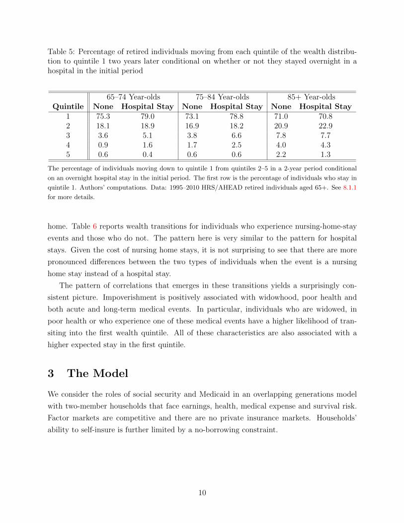
a hospital stay. Table 5 reports wealth mobility transitions to the first wealth quintile
for individuals who experience a hospital stay and those who do not. Hospital stays are
associated with an increased frequency of transitions to quintile 1. The differences here are
weaker compared to some of the previous indicators with two ties and one reversal. But the
impoverishing effect of a hospital stay is clearly discernible in Table 5. Quintile 1 is also a
more persistent state conditional on a hospital stay event for the two youngest age groups.
Given that acute medical expenses are transient in nature, it is not surprising at all to see
that the pattern of impoverishment is a bit weaker here as compared to e.g. self-reported
health status.
Finally, consider long-term care. Nursing home expenses are the largest long-term care
expense. The cost of a one-year stay in a nursing home can easily exceed $60, 000 and
while the average duration is only approximately two years, Brown and Finkelstein (2008)
estimate that approximately 9% of entrants will spend more than five years in a nursing
4See 8.1 for a description of our health variable.
9
Table 5: Percentage of retired individuals moving from each quintile of the wealth distribu-tion to quintile 1 two years later conditional on whether or not they stayed overnight in ahospital in the initial period
home. Table 6 reports wealth transitions for individuals who experience nursing-home-stay
events and those who do not. The pattern here is very similar to the pattern for hospital
stays. Given the cost of nursing home stays, it is not surprising to see that there are more
pronounced differences between the two types of individuals when the event is a nursing
home stay instead of a hospital stay.
The pattern of correlations that emerges in these transitions yields a surprisingly con-
sistent picture. Impoverishment is positively associated with widowhood, poor health and
both acute and long-term medical events. In particular, individuals who are widowed, in
poor health or who experience one of these medical events have a higher likelihood of tran-
siting into the first wealth quintile. All of these characteristics are also associated with a
higher expected stay in the first quintile.
3 The Model
We consider the roles of social security and Medicaid in an overlapping generations model
with two-member households that face earnings, health, medical expense and survival risk.
Factor markets are competitive and there are no private insurance markets. Households’
ability to self-insure is further limited by a no-borrowing constraint.
10
Table 6: Percentage of retired individuals moving from each quintile of the wealth distribu-tion to quintile 1 two years later conditional on whether or not they spent time in a nursinghome (NH) in the initial period
The percentage of individuals moving down to quintile 1 from quintiles 2–5 in a 2 year period conditional on
a nursing home stay in the initial period. The first row is the percentage of individuals who stay in quintile
1. Authors’ computations. Data: 1995–2010 HRS/AHEAD retired individuals aged 65+. See 8.1.1 for more
details.
3.1 Demographics
Time is discrete. The economy is populated by overlapping generations of households. Pop-
ulation grows at a constant rate n. Newborns are assigned to two-member households at age
1. Each member is endowed with a gender and an education type. We use xis to denote the
fraction of individuals of gender i ∈ m, f with either high school or college educational
attainment s ∈ hs, col. The distribution of households across education types s ≡ (sm, sf )
is Γs.
Each individual works during the first R periods of his/her life. We assume that all
working-age individuals are married. Individuals retire at age R + 1 and become subject to
survival risk. Thus retired households consist of either married couples, widows or widowers.
Marital status of a household is described by the variable d: d = 0 for married, d = 1 for a
widow and d = 2 for a widower. Individuals die no later than at age J .
3.2 The Structure of Uncertainty
The sources of uncertainty vary by age. Working individuals are only exposed to earnings
risk. At retirement, individuals face survival and health risk and households face medical
expense risk. We describe each of these risks in detail.
Individual productivity evolves over the working period according to functions Ωi(j, εe, si),
i ∈ m, f, that map individual age j, household earning shocks εe ≡ (εme , εfe ) and education
type si into efficiency units of labor. The vector of household earning shocks εe follows an
11
age-invariant Markov process with transition probabilities given by Λee′ . Efficiency units of
newborn households are distributed according to Γe.
Starting at retirement, individuals face uncertainty about their health. An individual’s
health status, hi, takes on one of two values: good (hi = g) and bad (hi = b). The probability
of having good health next period, νij(h, d), depends on age, gender, current health status and
marital status. The initial distribution of health status, Γih(si), depends on the individual’s
education. Finally, denote a household’s health status by h ≡ (hm, hf ).
Medical and long-term care expenses are incurred at the household level and evolve
stochastically according to the function Φ(j,h, εM , d) that depends on household age j,
household health status h, the vector of medical expense shocks εM and demographic status
d. There are two medical expense shocks. The first shock follows an age-invariant Markov
process with transition probabilities ΛMM ′ and initial distribution ΓM1 . The second shock is
a transient, iid shock with probability distribution ΓM2 .
Upon reaching retirement age, individuals face survival risk. This risk has two compo-
nents. First, there is a death shock at age 65 which depends on that individual’s lifetime
earnings if male and their spouse’s if female. This shock is used when calibrating the model
to pin-down the age-65, marital status distribution Γd(e). The rationale for this assumption
is discussed in more detail in Section 4.1.3. Second, once retired, the probability of surviving
to age j+1 conditional on surviving to age j is given by πij(h, d) and depends on age, gender,
health status and marital status.
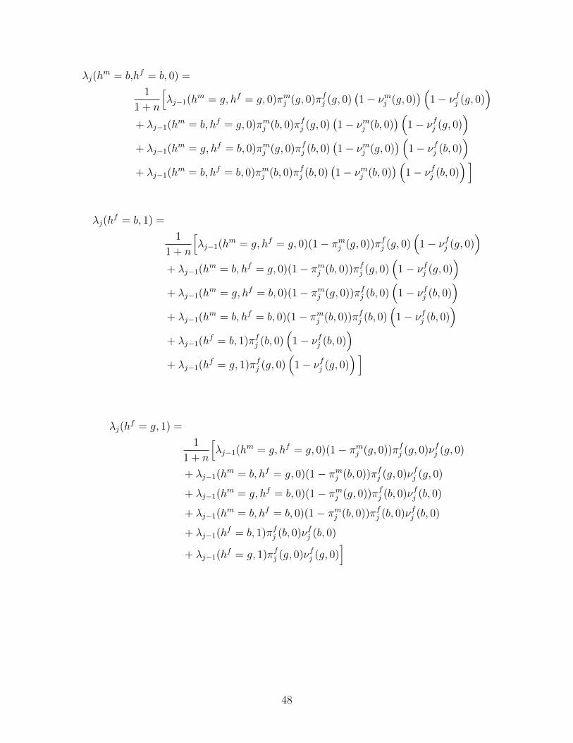
Given these definitions, denote the survival rate from j − 1 to age j of a household with
health and marital status of (h, d) by λj(h, d). The laws of motion for λj(h, d) are provided
in the Appendix. It follows that the size of cohort j is given by
ηj = ηj−1∑h
∑d
λdj (h, d), for j = 2, 3, ..., J.
.
3.3 Government
The government uses revenues from corporate, payroll and income taxes to finance SS pay-
ments, means-tested transfers and government expenditures, G.
3.3.1 Social Security
Currently, the U.S. Social Security system levies a payroll tax and uses its revenues to pay
full benefits to eligible workers who retire at age 65. The program also provides benefits to
12
spouses and survivors of eligible workers. We model SS as a pay-as-you go system.
Benefits In order to capture the spousal and survivor benefits, we assume that the benefit
function S(e, d) depends on lifetime earnings of both household members, e and the house-
hold’s current marital status, d. The specific benefit formula is reported in the Appendix.
We note here that it captures the following features of the U.S. Social Security system. First,
married couples have the option of either receiving their own benefits or 1.5 times the benefit
of the highest earner in the household. Second, widows/widowers have the choice of taking
their own benefit or their dead spouses benefit.
Sources of Finance The tax that finances SS benefits in the U.S. is a proportional tax
levied on individual earnings, or payroll, up to a specified ceiling. In our model, this payroll
tax is reflected by function τss(·), which we calibrate consistently with the U.S. Social Security
system.
3.3.2 Medicaid and Other Means-Tested Programs
Benefits Medicaid has grown into the largest means-tested program in the U.S. Its primary
beneficiaries are the elderly, the disabled, children and single women with children. The focus
of this paper is on Medicaid and other means-tested welfare for the elderly, so we discuss
benefits to the elderly first.
General guidelines for Medicaid benefits for the elderly are determined by the Federal
government. However, states establish and administer their own Medicaid programs and
determine the scope of coverage. For example, most states require copayments. The size of
copayments varies depending on the type and amount of the expense incurred. In addition,
some States cover prescription drugs, hearing aids and eye glasses, other States do not. A
result is that many Medicaid recipients still have significant OOP expenses.5
Retirees may qualify for other means-tested welfare benefits including Supplemental So-
cial Security Income, subsidized housing, food stamps and energy assistance. The federal
government determines the Supplemental Social Security Income eligibility and most states
use the same means test to determine eligibility for Medicaid and other state-run welfare
programs. We choose to model these programs using a single means-tested transfer:
5A third reason that we see significant OOP expenses is that there is a medically needy path to Medicaid.See De Nardi, French and Jones (2012) for more discussion of this path to Medicaid.
13
TrR ≡
max
yd + ϕM − IR, cd +M − IR, 0
, if yd > IR −M,
0, otherwise.(1)
Equation 1 describes the various situations that a retired household can find itself in. If
its cash-in-hand, IR, net of medical expenses, M , exceeds the means-test income threshold
yd, the household receives no Medicaid benefits. If the household’s cash-in-hand net of
medical expenses falls below yd, it does receive a Medicaid benefit but is responsible for a
Medicaid copayment of (1 − ϕ)M . However, we cap this copayment in a way that insures
that the household’s consumption is at least cd.
In our model working households do not face medical expenses. We thus abstract from
Medicaid for them. However, working households do face earnings risk and we model means-
tested transfers that are a stand-in for programs such as unemployment insurance and food-
stamps. Let IW denote cash-in-hand for a working household, then the transfer is
TrW ≡ max
0, c− IW, (2)
where c is the consumption floor.
Sources of Finance Medicaid and other means-tested social welfare programs are jointly
financed by states and the federal government using a variety of revenue sources. In the
model, we assume that all funding for means-tested transfers comes out of general government
revenues.
3.3.3 Medicare and Government Purchases
Medicare outlays are financed by a payroll tax τmc. It follows that total payroll taxes are
τe(e) = τss(e) + τmc(e). We do not formally model the distribution of Medicare benefits.
The main reason for this is a lack of data on individual or household level Medicare benefits.
HRS only reports post-Medicare OOP medical expenses. In our model, medical expenses
covered by Medicare are included in government purchases, G, instead.
The government budget is balanced period-by-period. It follows that revenues from the
corporate tax τc, income taxes TWy and TRy , and Medicare tax τmc(·) finance means-tested
transfers and G.
14
3.4 Household’s Problem
We start by describing the household’s preferences. For married households, most of the
variation in labor supply is due to changes in labor force participation and hours worked by
the female (see e.g. Keane and Rogerson (2012) for a survey). For this reason, we abstract
from the male labor supply decision but model both margins of labor supply by the female.
We assume that households have preferences over consumption c and non-market time of
the female member lf .
The utility function of a working household is given by
UW (c, lf , s) = 2N−1(c/(1 + χ)N−1
)1−σ1− σ
+ ψ(s)l1−γf
1− γ− φ(s)I(lf < 1), (3)
where N is the number of living household members (N = 2 for all working households), I is
the indicator function, σ, γ > 0 and ψ(s), φ(s) > 0 for all s. This specification of preferences
assumes a unitary household in which each member is fully altruistic towards their spouse.
The parameter χ ∈ [0, 1] determines the degree to which consumption is joint within the
household. For instance, when χ is 1, all consumption is individual and when χ is 0, all
consumption is joint. The third term in the utility function captures the utility cost of
female participation in the labor force. Modeling this cost helps us match both the intensive
and extensive margins of female labor supply.
The utility function of a retired household with N living members (determined by d) is
defined similarly:
UR(c, d) = 2N−1(c/(1 + χ)N−1
)1−σ1− σ
+ ψRl1−γf
1− γ, (4)
where lf = 1 and ψR > 0.
The constraints and decisions of working households and retired households are quite
different. We thus describe each problem separately.
3.4.1 Working Household’s Problem
A working household of age j with education type s ≡ sm, sf enters each period with
assets a and average lifetime earnings of the male and female e ≡ em, ef. It then receives
the current labor productivity shocks εe ≡ εme , εfe and chooses consumption c, savings a′
and female labor supply lf . Let earnings be ei = wΩi(j, εe, si)(1 − lIi=f ), i ∈ m, f. The
15
optimal choices are given by the solution to the following problem:
V W (j, a, e, εe, s) = maxc,lf ,a′
UW (c, lf , s) + βE
[V (j + 1, a′, e′, ε′e, s)|εe
], (5)
subject to the law of motion for εe and its initial distribution, as described in Section 3.2,
and the following constraints:
c ≥ 0, 0 ≤ lf ≤ 1, a′ ≥ 0, (6)
ei′ = (ei + jei)/(j + 1), i ∈ m, f, (7)
c+ a′ = a+ yW − TWy + TrW , (8)
where
yW ≡ em + ef + (1− τc)ra, (9)
TWy ≡ τy(yW − τe(em)em − τe(ef )ef
)+ τe(e
m)em + τe(ef )ef , (10)
IW ≡ a+ yW − TWy . (11)
Equation (6) describes regularity conditions on consumption and leisure and imposes a bor-
rowing constraint which rules out uncollateralized lending. The dynamics of average lifetime
earnings, which determine social security benefits, are given in (7) and the household budget
constraint is given by (8). The definition for TrW is given in (2). Household income (9) has
two components: labor income and capital income. Capital income is subject to a corporate
tax τc, and (10) states that households also pay an income tax τy() and a payroll tax, τe(e).
Finally, (11) defines cash-in-hand.
3.4.2 Retired Household’s Problem
During retirement the household’s problem changes. Men and women spend all of their time
endowment enjoying leisure. Retirees face health, medical expense and survival risk.
We will assume that individuals observe their own and their spouses death event one
period in advance. It follows that bequests are zero for households with a single member.
16
This assumption has the following motivations. First, there is considerable evidence that
bequests and inheritances are low. One reason for this is that wealth is low in the final year
of life. Poterba, Wise and Venti (2012) find that many individuals die with very low levels
of assets. They report that 46.1% of individuals have less than $10,000 in financial assets in
the last year observed before death and 50% have zero home equity using data from HRS.
In a separate study of the Survey of Consumer Finances (SCF) Hendricks (2001) reports
direct measurements of inheritances. He finds that most households receive very small or
no inheritances. Fewer than 10% of households receive an inheritance larger than two mean
annual earnings and the top 2% account for 70% of all inheritances.
The second reason for this assumption is that it allows us to capture the fact that both
OOP and Medicaid medical expenses are large in the final year of life. In our HRS sample
of retirees, OOP expenses in the last year of life are 3.43 times as large as OOP expenses
in other years. Medicaid expenditures are not available in our dataset. However, Hoover et
al. (2002) report that in final year of life Medicaid expenditures are 25% of total Medicaid
expenditures for those aged 65 and older. This result is based on Medicare Beneficiary
Survey data from 1992–1996.
An attractive outcome of this assumption is that accidental bequests are zero. Previous
research has found that the pattern of redistribution of accidental bequests has important
incentive effects. Changes in government policy that alter the size and distribution of these
bequests have big incentive effects and this acts to muddle any analysis of the welfare effects
of policy reform. For examples of this see Kopecky and Koreshkova (2007) and Hong and
Rıos (2007).
For retirees the household’s education type is no longer a state variable. Education does
enter indirectly since the initial distribution of individual health status varies with educa-
tional attainment. Health, and thus education, affect both individual survival probabilities
and household medical expenses as described in Section 3.2.
The probability that an age-j individual of gender i with health status hi and marital
status d survives to age j + 1 is denoted by πij+1(hi, d). It follows that an age-j household
faces survival probabilities πj(d′|h, d) given by
d′ = 0 d′ = 1 d′ = 2
d = 0 πmj+1(hm, 0)πfj+1(h
f , 0)[1− πmj+1(h
m, 0)]πfj+1(h
f , 0) πmj+1(hm, 0)
[1− πfj+1(h
f , 0)]
d = 1 0 πfj+1(hf , 1) 0
d = 2 0 0 πmj+1(hm, 2)
An age-j household with assets a, average lifetime earnings e, health h, medical expense
17
shock εM , current demographic status d and next period demographic status d′ chooses c
and a′ by solving
V R(j, a, e,h, εM , d, d′) = maxc,a′
UR(c, d)+βE
[ 2∑d′′=0
πj(d′′|h′, d′)V (j+1, a′, e,h′, ε′M , d
′, d′′)|h, εM]
(12)
subject to the laws of motion for h, εM and their initial distributions, as described in Section
3.2 and the following constraints:
c ≥ 0, a′ ≥ 0, (13)
c+M + a′ = a+ yR − TRy + TrR, (14)
where
M ≡ Φ(j,h, εM , d, d′), (15)
yR ≡ S(e, d) + (1− τc)ra, (16)
TRy ≡ τRy ((1− τc)ar, S(e, d), d,M) , (17)
IR ≡ a+ yR − TRy , (18)
and the expectations operator E is taken over ε′M and h′. The means-tested transfer TrR is
defined in equation (1).
The main differences between the working household’s problem and the retired house-
hold’s problem are as follows. Medical expenses M now enter the household’s budget con-
straint (14). Households have no labor income but instead may receive social security bene-
fits. Retired households also face a nonlinear income tax schedule. In particular, their social
security benefits are also subject to income taxation if these benefits exceed the exemption
level specified in the U.S. tax code. We also allow for a deduction of medical expenses that
exceed κ percent of taxable income. The specific formulas used to compute income taxes are
reported in the appendix.
18
3.4.3 Problem for a Household about to Retire
The previous two cases cover all situations except that of a household in its last working
period, R. Such a household enters the period with the state variables of a working household
and chooses consumption, savings and female labor supply, recognizing that in period R+ 1
it will face the problem of a retired household. Consequently, when evaluating next period’s
value function, they form expectations using the distributions Γmh , Γfh, ΓM1 , ΓM2 and Γd(em).
3.5 Technology
Competitive firms produce a single homogeneous good by combining capital K and labor L
using a constant-returns-to-scale production technology:
Y ≡ F (K,L) = AKαL1−α,
and rent capital and labor in perfectly competitive factor markets. The aggregate resource
constraint is given by
Y + (r + δ)(K −K) = C + (1 + n)K ′ − (1− δ)K + M +G,
where K is per capita private wealth, C denotes per capita consumption, M is per capita
medical expenses, G is government purchases and δ is the depreciation rate on capital.
3.6 General Equilibrium
We consider a steady-state competitive equilibrium for a small open economy.6 For the
purposes of defining an equilibrium in a compact way, we suppress the individual state into
a vector (j, x, d, E), where
x =
xW ≡ (a, e, εe, s), if 1 ≤ j ≤ R,
xR ≡ (a, e,h, εM , d, d′), if R < j ≤ J,
Accordingly, we redefine value functions, decision rules, income taxes, means-tested transfers
and SS benefits to be functions of the individual state (j, x):V W (j, x), V R(j, x), c(j, x),
6Even though the U.S. is a large economy, capital markets are integrated and thus it is not clear howimportant changes in domestic savings are for determination of the real interest rate. We therefore chooseto hold the real interest rate fixed.
19
a′(j, x), lf (j, xW ), Ty(x), Tr(j, x) and S(xR). Define the individual state spaces:
and denote by Ξ(X) the Borel σ-algebra on X ∈ XW , XR. Let Ψj(X) be a probability
measure of individuals with state x ∈ X in cohort j. Note that these agents constitute a
fraction ηjΨdj (X) of the total population.
DEFINITION. Given a fiscal policy S(e, d), G, τc, τmc(e), cd, yd, κ and a real interest
rate r, a steady-state competitive equilibrium consists of household policies c(j, x), a′(j, x), lf (j, x)Jj=1
and associated value functions V W (j, x)Rj=1, V R(j, x)Jj=R+1, taxes and prices τss(e), Ty(x), w,per capita capital stocks K,K and an invariant distribution ΨjJj=1 such that
1. At the given prices and taxes, the household policy functions c(j, x), a′(j, x) and l(j, x)
achieve the value functions.
2. At the given prices, firms are on their input demand schedules: w = FL(K,L) and
r = FK(K,L)− δ.
3. Aggregate savings are given by∑
j ηj∫Xa′(j, x)dΨj = (1 + n)K.
4. Markets clear:
(a) Goods∑
j ηj∫Xc(j, x)dΨj +(1+n)K+M+G = F (K,L)+(1−δ)K+r(K−K),
where M =∑J
j=R ηj∫XR
Φ(j,h, εM , d, d′)dΨj.
(b) Labor:∑
j ηj∫X
(1− lf (j, x))Ωf (j, εe, s
f ) + Ωm(j, εe, sm)dΨj = L.
5. Distributions of agents are consistent with individual behavior:
Ψj+1(X0) =
∫X0
∫X
Qj(x, x′)Ij′=j+1dΨj
dx′,
for all X0 ∈ Ξ, where I is an indicator function and Qj(x, x′) is the probability that
an agent of age j and current state x transits to state x′ in the following period. (A
formal definition of Qj(x, x′) is provided in the Appendix.)
6. SS budget is balanced: SSbenefits = PayrollTaxes, where
The model is parameterized to match a set of aggregate and distributional moments for the
U.S. economy, including demographics, earnings, medical and nursing home expenses, as
well as features of the U.S. social welfare, Medicaid, social security and income tax systems.
Some of the parameter values can be determined ex-ante, others are calibrated by making the
moments generated by a stationary equilibrium of the model target corresponding moments
in the data. The calibration procedure minimizes the differences between the data targets
21
6 5 7 0 7 5 8 0 8 5 9 0 9 50
2 0
4 0
6 0
8 0
1 0 0h e a l t h y , s i n g l e m a l e s
u n h e a l t h y , s i n g l e m a l e s
h e a l t h y , m a r r i e d m a l e s
u n h e a l t h y , m a r r i e d m a l e s
h e a l t h y , m a r r i e d f e m a l e s
u n h e a l t h y , m a r r i e d f e m a l e s
h e a l t h y , s i n g l e f e m a l e s
Perce
nt
A g e
u n h e a l t h y , s i n g l e f e m a l e s
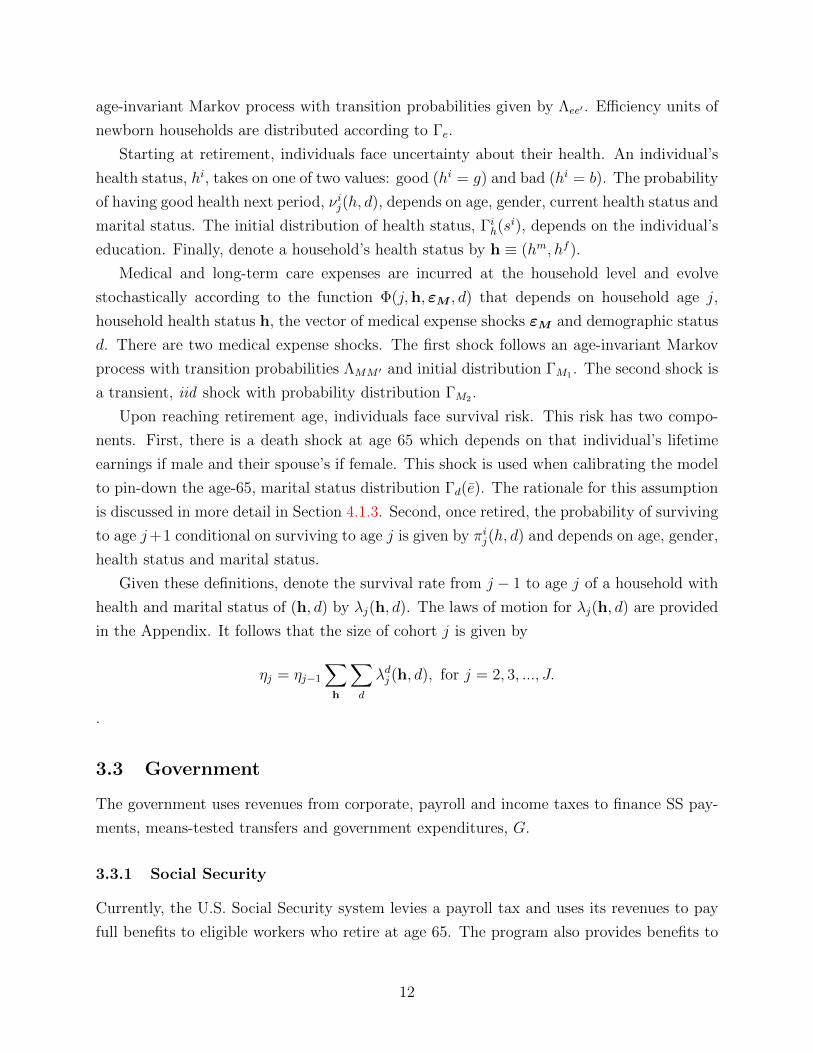
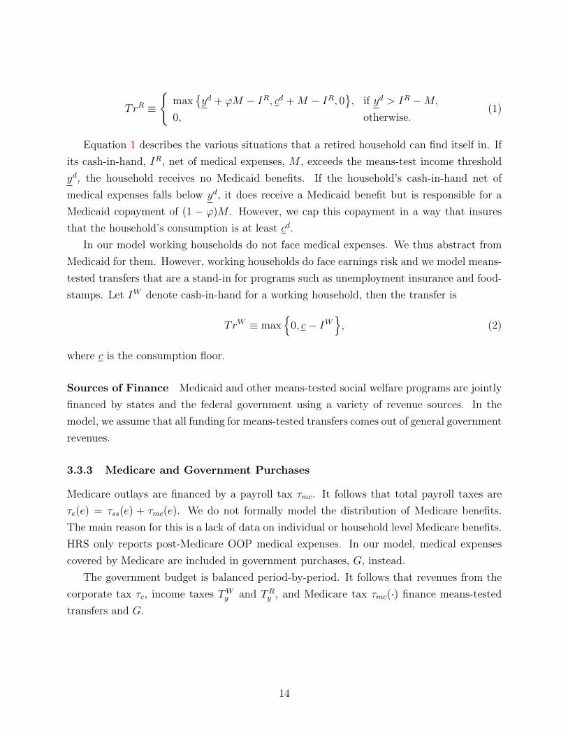
Figure 1: The population distribution of retirees by age. Individuals are classified by gender,health and marital status. The data for this figure is our HRS sample.
and model’s predicted values.7 We focus in this section on the most important aspects of
the calibration. Additional calibration details are proved in Section 8.3.
4.1 Demographics
This section reports how we calibrate the parameters of the model that pertain to demo-
graphics. Agents are born at age 21 and can live to a maximum age of 100. Given that the
focus of our analysis is on retirees, we want to reproduce the demographic structure of those
65 and older. Figure 1 reports the evolution of the distribution of retirees by marital status,
health and gender estimated from our HRS sample. At the beginning of retirement, half of
the population is healthy and married. As individuals age, three things happen: the fraction
of singles increases, the fraction of unhealthy increases and males die faster than females.
Below we will describe how we estimate this demographic structure and build it into our
model.
7Due to the computational complexity of the model it is not feasible to implement a formal method-of-moments estimation strategy.
22
4.1.1 Age Structure
We set the model period to two years because the data on OOP medical expenses is only
available bi-annually. The maximum life span is J = 40 periods. Agents work for the first
44 years of life, i.e. the first 22 periods. At the beginning of period R + 1 = 23, they retire
and begin to face survival risk.
The target for the population growth rate n is the ratio of population 65 years old and
over to that 21 years old and over. According to U.S. Census Bureau, this ratio was 0.18 in
2000. We target this ratio rather than directly setting the population growth rate because
the weight of the retired in the population determines the tax burden on workers, which is
an object of primary interest in our policy analysis. The resulting annual growth rate of
population is 1.8 percent.
4.1.2 Education
Newborn are endowed with either high school or college educational attainment which is fixed
throughout their working life. The model distribution of schooling types is set to reproduce
its empirical counterpart in our HRS data sample for 65–66 year-old married households. In
our data, both spouses have college degrees in 14 percent of households, in 14 percent only
the male has a college degree, in 5 percent only the female has a college degree, and in 67
percent neither spouse has a college degree.
4.1.3 Marital Status
Newborn are matched with a spouse and remain married until at least age 65. In our HRS
sample, only 48 percent of 65–66 year-olds households are married couples, 36 percent are
single females and 16 percent are single males. For the most part, these figures reflect the
cumulative effects of divorce and spousal death in the ages prior to age 65. Since our primary
objective is to model retirees, we summarize these effects with a spousal death event at age
65. This event, which is distinct from the health-related survival risk agents face throughout
retirement, ensures that Γd(e) reproduces the marital status distribution of 65 year-olds in
the data.
Another feature of our HRS data is that social-security income varies with martial status.
Table 7 shows that there are very large differences in social security benefits across the three
types of households. Married households have the highest benefits and single males receive
higher benefits than females. In order to reproduce these observations, we assume that the
spousal death shock has a negative relation with the distribution of average life-time earnings
of the male. We then calibrate the death shock so that it reproduces the fractions of married,
23
Table 7: Marital status distribution of households with 65–66 year-old household heads bysocial security benefit quintiles
Quintile1 2 3 4 5
Married 0.19 0.24 0.36 0.67 0.95Single Female 0.56 0.55 0.45 0.21 0.03Single Male 0.25 0.21 0.20 0.12 0.02
The fraction of households in each social security income quintile who are married, single female or single
male households. Authors’ computations. Data: 1995–2010 HRS/AHEAD retired households aged 65+. See
8.1.1 for more details.
single male and single female households by social security benefit quintiles shown in Table
7.
4.1.4 Survival Probabilities and Health Status
Table 8 reports estimates of expected remaining years of life for 65-year-old individuals by
marital status, health status and gender. All three factors have large effects on longevity.
Having a spouse at age 65 is particularly beneficial for males extending their longevity by
2.9 years compared to 1.7 years for females. Good health extends life by about five years for
both genders. Finally, females live on average 2.9 years longer than males.
These results are based on estimated survival probabilities, πij+1(hi, d), for males and
females from our HRS sample. Survival probabilities are assumed to be a logistic function of
age, age-squared, health status, marital status, health status interacted with age and marital
status interacted with age. Transition probabilities for health status are also estimated
separately for males and females, using the same logistic functions. The initial distributions
of individuals across health status at age 65, Γih(si), are set to match the distribution of
health status by education in the HRS sample for 65–66 year-olds.
4.2 Medical Expense Process
Medical expenses vary systematically with age, gender, health and marital status. Moreover,
when motivating our model, we found evidence that suggested medical expense shocks are
important sources of impoverishment for retirees. We assume the medical expenses have a
deterministic and stochastic component. We now describe each of these components.
24
Table 8: Expected additional years of life at age 65 by health status, marital status andgender
Female Male All
19.5 16.6 18.2
By healthgood 20.5 17.6 19.2bad 15.8 12.2 14.3
By marital statusmarried 20.1 17.2 18.6single 18.4 14.3 17.0
Authors’ computations. Data: 1995–2010 HRS/AHEAD retired households aged 65+. See 8.1.1 for moredetails on the data. Note that life expectancies in our HRS sample are lower than those in the 2000 U.S.Census. We thus scaled up the survival probabilities to match Census life expectancies at age 65.
4.2.1 Deterministic Medical Expense Profiles
In the model, medical expenses are household-specific. We start by estimating deterministic
medical expense profiles for individuals and then sum these expenses over spouses for married
couples. The shape of the medical expense profiles is determined by regressing individual
medical expenses on a quartic in age and a quartic in age interacted with gender, marital
status, mortality status (a dummy variable that takes on the value of one if death occurs in
the next period) and health status using a fixed-effects estimator.8
Our HRS data only reports household expenses paid out of pocket and not those covered
by Medicaid. However, when solving the model, we need to specify pre-Medicaid medical
expenses, defined as the sum of OOP and Medicaid payments. To resolve this issue, we
exploit the fact that individuals in the top lifetime earnings quintile (or who have/had
spouses in the top lifetime earnings quintile) are unlikely to be eligible for means-tested
Medicaid transfers, and hence their OOP medical expenses are, on average, very close to
their pre-Medicaid expenses. Thus, the control variables in our medical expense regression
include permanent income quintile dummies and their age-interaction terms. These latter
controls reduce the estimation bias arising from the fact that Medicaid transfers increase
with age. The estimated coefficients from this regression for permanent earnings quintile
5 pin down the shape of the deterministic age-profile of the pre-Medicaid medical expense
8As pointed out by De Nardi et al. (2010), the fixed effects estimator overcomes the problem with thevariation in the sample composition due to differential mortality as well as accounts for cohort effects.
25
6 5 7 0 7 5 8 0 8 5 9 0 9 5 1 0 01 . 0
1 . 1
1 . 2
1 . 3
1 . 4
1 . 5
1 . 6
1 . 7
H e a l t h : B a d / G o o d
M a r r i e d : D Y / N o t D Y
S i n g l e / M a r r i e d
F e m a l e / M a l e
Ratio
of m
edica
l exp
ense
s
A g e
S i n g l e s : D Y / N o t D Y
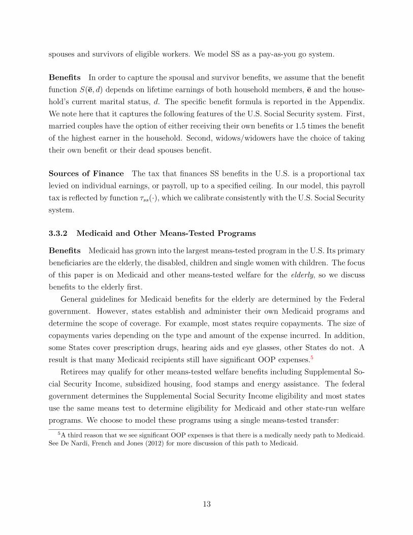
Figure 2: Estimated effects of marital status, health and death year (DY) conditional onmarital status on individual medical expenses by age. The vertical axis is the ratio ofestimated medical expenses for each type pair. Data: 1995–2010 HRS/AHEAD retiredindividuals aged 65+. See 8.1 for more details.
process.9
The obtained medical expense profiles are similar to profiles reported in De Nardi et
al. (2010) and Kopecky and Koreshkova (2007). OOP expenses increase with permanent
income and age. Moreover, OOP medical expenses are higher for females relative to males
and higher if self-reported health status is poor.
Our estimated medical expense profiles also provide new information about how medical
expenses vary by marital status and death year. Figure 2 shows the effects of marital status
and death year on medical expenses. For purposes of comparison, we also report how medical
expenses vary with gender and health. The most striking feature of the figure is that death
year has a very large effect on medical expenses and its importance increases with age. At
age 65 medical expenses for singles in their death year are 15% higher than for singles not
in their death year. By age 85 the difference has risen to 45%. The effect of death year
is smaller for married individuals but still important. A second result is that the effect of
marital status on medical expenditures is as large as or larger than the effect of health for
those under age 95.
9All of the coefficients documented here are significant at conventional significance levels. Estimatedcoefficients and standard errors from these regressions are available upon request.
26
4.2.2 Stochastic Structure of Medical Expenses
The stochastic component of medical expenses has a persistent and a transitory component.
The standard deviation of the transitory component is 0.816 and the persistent component
is assumed to follow an AR(1) at annual frequencies with an autocorrelation coefficient of
0.922 and a standard deviation of 0.579. These values are taken from French and Jones
(2004).10 The initial distribution of the persistent medical expense shock, ΓM1 , is set to the
distribution of OOP expenses at age 65–66 in our HRS data sample.
Previous work has found that an important source of variation in retirees medical ex-
penses is long-term care needs.11 To capture long-term care risk, we approximate the per-
sistent shock with a five state Markov chain. In particular, we assume that the fifth state
is associated with nursing home care. This calibration of the Markov chain captures both
the small variation in medical expenses due to acute costs and the large variation due to
long-term care costs. In particular, we target data facts pertaining to expected duration of
nursing home stays, the distribution of age at first entry and overall size of nursing home ex-
penses. The resulting Markov process recovers the serial correlation and standard deviation
of the AR(1) process but is not Gaussian. More details on this aspect of the calibration are
reported in 8.3.1.
Finally, we scale the medical expense profiles so that aggregate medical expenditures in
the model are 2.1% of GDP. This target corresponds to the average total expenditures on
medical care paid OOP or by Medicaid during the period 1999 to 2005.12
4.3 Government
We divide our discussion of the calibration of fiscal policy variables into two parts. We start
by discussing calibration of the sources of government revenue and then turn to discuss the
uses of government revenue.
4.3.1 Sources of Government Revenue
The government raises revenue from three taxes: a proportionate corporate profits tax, and
nonlinear income and payroll taxes. We choose the size of the corporate profits tax and
income taxes to reproduce the revenues of each of these taxes expressed as a fraction of
10Their estimates are based on individuals. We use these values for the household but assume that themedical expense shocks to husbands and wives are independent.
11See for example Kopecky and Koreshkova (2007) who find that nursing home expenses are importantdrivers of life-cycle savings.
12Total medical expenditures paid OOP or by Medicaid are taken from the “National Health ExpenditureAccounts,” U.S. Centers for Medicare and Medicaid Services and include payments for insurance premia.
27
GDP in U.S. data. The specific targets are 2.8% of GDP for the corporate profits tax and
8% of GDP for the income tax. These targets are averages over years 1950–2008 as reported
in Table 11 of “Present Law and Historical Overview of the Federal Tax System.”
U.S. income tax schedules vary with marital status. In our model, all workers are married
but retirees can be single or married. Using the IRS Statistics of Income Public Use Tax
File for the year 2000, Guner, Kaygusuz and Ventura (2012) estimate effective income tax
functions for both married households and singles following the methodology of Kaygusuz
(2010). We use their estimates (see Section 8.3.5 for more details.).
Contributions for SS and Medicare are financed by the payroll tax, τe = τss+τmc. The SS
component of this tax, τss is subject to a cap. We set the cap to be twice average earnings.
This choice reproduces the cap of $72, 000 for the year 2000 in U.S. data. The Medicare
component of this tax, τmc, is set to the total (employee + employer) Medicare tax rate
which in year 2000 was equal to 2.3%.
4.3.2 Uses of Government Revenue
Recall that the government has three principal uses of funds: it pays social security benefits
to retirees, provides means-tested social welfare benefits, and purchases goods and services
from the private sector. We discuss the calibration of each of these types of expenditures in
turn. The social security benefit function in our model reproduces the progressivity of the
U.S. social security system and provides spousal and survivor benefits (see 8.3.6 for details).
The welfare program in our model represents public assistance programs in the U.S., in-
cluding Medicaid, Supplemental Social Security Income, food stamps, unemployment insur-
ance, Aid to Families with Dependent Children, and energy and housing assistance programs.
For working individuals, we set the consumption floor, c, in equation (2) to 15% of average
earnings of full-time, prime-age, male workers. In year 2000 dollars, this is approximately
$7,100. This magnitude is consistent with estimates from the previous literature.13
The means-test income thresholds yd and consumption floors cd, of retirees vary with
marital status. We set the consumption floors to 1/2 the level of the income thresholds
and then set the income thresholds to target Medicaid take-up rates for retirees in our
HRS dataset. The values of the targets are 22% for widows, 17% for widowers and 7% for
married individuals. The resulting means-test income thresholds are close to 32% of average
earnings of full-time, prime-age, male workers for all three types of individuals.14 That is,
they are approximately $15,200 in year 2000 dollars. It follows that the consumption floors
for retirees are about 16% of male average earnings or approximately $7,600. The target for
13See Kopecky in Koreshkova (2007) for a discussion of the literature on consumption floors.14The precise values are y0 = 0.31, y1 = 0.33 and y2 = 0.32.
28
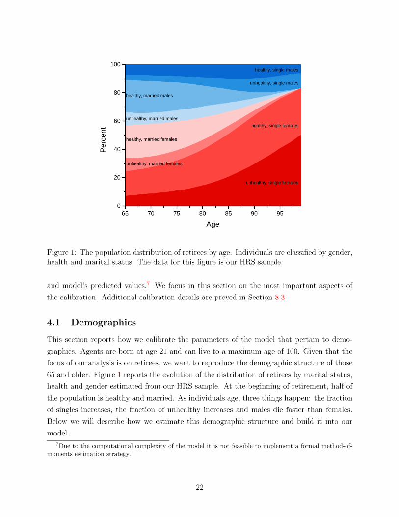
Table 9: Medicaid take-up rates by age and marital status
Age 65–74 75–84 85+
Marital StatusMarried
data 0.07 0.07 0.11model 0.05 0.07 0.12
Widowsdata 0.22 0.19 0.24model 0.21 0.23 0.25
Widowersdata 0.19 0.15 0.19model 0.17 0.16 0.17
The fraction of individuals receiving Medicaid transfers by age group and marital status in the data and the
model. Data: 1995–2010 HRS/AHEAD retired individuals aged 65+. See 8.1 for more details.
the Medicaid copay rate, (1−ϕ), is the ratio of average OOP medical expenses of Medicaid
recipients to average OOP medical expenses of all retirees. In our HRS sample, this ratio is
0.46. The resulting copay rate is 20%.
Finally, we adjust government purchases, G, of goods and services to close the government
budget constraint. This results in a G/Y ratio of 0.11 for our baseline parameterization of
the model.
5 Assessment of Baseline Calibration
In this section we compare some moments from the model with the data that were not tar-
geted when parameterizing the model. We start by showing that the model delivers patterns
close to the data on Medicaid take-up rates, flows into Medicaid and OOP medical expenses
by age and marital status. Then we show that the model delivers an increased likelihood
of impoverishment for individuals with large acute and long-term care OOP expenses, bad
health status and those whose spouse has died, in line with the evidence on impoverishment
documented in Section 2.
5.1 Medicaid Take-up Rates and Flows
We start by discussing Medicaid take-up rates. In calibrating the model, we set the con-
sumption floors to reproduce the fractions of each type of retired household on Medicaid.
29
Table 10: Bi-annual Flows into Medicaid by Age and Marital Status
The flows are the fraction of retirees with given initial marital status not receiving Medicaid but who become
recipients over the next two years. Data: 1995–2010 HRS/AHEAD retired individuals aged 65+. See 8.1
for more details.
The Medicaid take-up rates by age were not explicitly targeted and thus are a way to assess
the model’s performance. Table 9 compares the take-up rates of Medicaid by age for the
three household types. Inspection of Table 9 indicates that the model does a good job of
reproducing Medicaid take-up rates for each age group.
Another implication of the model that was not targeted is flows into Medicaid. Table
10 reports flows into Medicaid by age and marital status. Observe that in the data, the
flows into Medicaid are much lower for married than singles. Moreover, the flows increase
monotonically with age for married but follow a U-shaped pattern for singles. Model flows
into Medicaid reproduce all of these features of the data. The model also reproduces the
magnitudes of the flows into Medicaid for married households, although it overstates the
flows of widows aged 65–74. This may be due to the fact that we do not allow people
to qualify for Medicaid before age 65 in the model. In the data some widows qualify for
Medicaid before age 65 and thus the flow at age 65 is lower.
5.2 Out-of-pocket medical expenses
Figure 3 reports OOP medical expenses of households in the data and the model by marital
status and social security income quintile. De Nardi et al. (2006) show that OOP medical
expenses of single individuals are increasing by permanent income quintile.15 Consistent with
15De Nardi et al. (2006) use annuitized income to proxy for permanent income. Constructing annuitizedincome for households is subtle. So we use social security income instead. It is the largest component of
30
OO
P E
xpen
ses
0
0.5
1
1.5
2
Social Security Income Quintile1 2 3 4 5
OO
P E
xpen
ses
0
0.5
1
1.5
2
Social Security Income Quintile1 2 3 4 5
model
model
model
data
data
data
O
OP
Exp
ense
s
0
0.5
1
1.5
2
Social Security Income Quintile1 2 3 4 5
Single Males
Married Couples Single Females
Figure 3: Out-of-pocket health expenses of married couples (top, left), single females (top,right) and single males (bottom) relative to mean OOP expenses of all households by socialsecurity income quintile in the model (red squares) and the data (blue circles).
these findings, Figure 3 shows that household’s OOP expenses increase with social security
income in the data. Observe that OOP expenses also increase with social security income in
the model. The primary reason for this is that, as income increases, the fraction of medical
expenses covered by Medicaid falls. If the increase in OOP expenses with income in the
data is, at least, in part due to wealthier households purchasing more quantity or quality of
care, one might expect the model to understate OOP expenses of high income households.
However, the model actually overstates OOP expenses of high income widowers and widows.
We believe that these gaps are due to the fact that in the model there is no medically-needy
path to Medicaid. In the data, some high income household are eligible for Medicaid under
this path and have reduced OOP expenses as a result.16
5.3 Probability and Persistence of Impoverishment
We next discuss how well the model reproduces the differentials in downward mobility dis-
cussed in Section 2. Recall that we found evidence in the data that singles face a higher
probability of impoverishment as compared to married individuals and that poverty is a more
annuitized income and we can observe it at the household level in both the model and the data.16Source: Kaiser Commission on Medicaid and the Uninsured, December 2012.
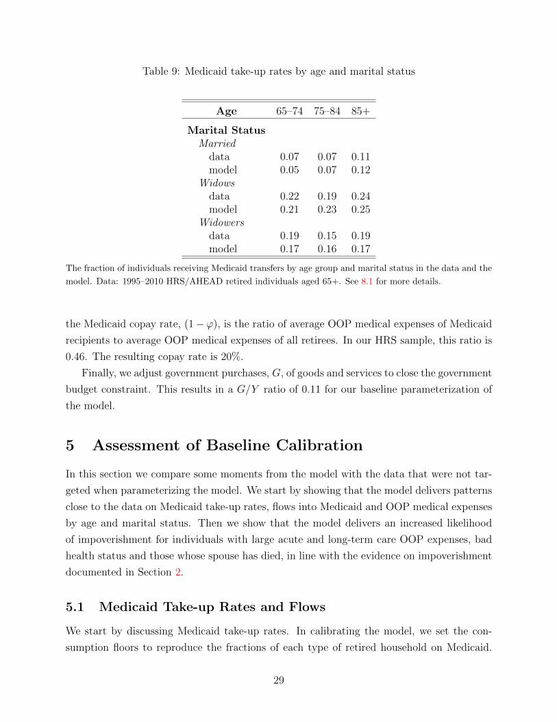
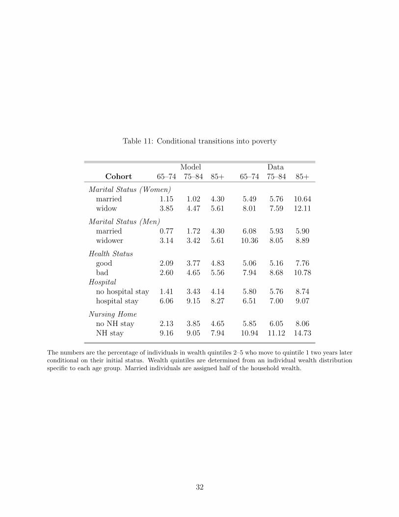
The numbers are the percentage of individuals in wealth quintiles 2–5 who move to quintile 1 two years laterconditional on their initial status. Wealth quintiles are determined from an individual wealth distributionspecific to each age group. Married individuals are assigned half of the household wealth.
The numbers are the percentage of individuals in wealth quintile 1 who are still in quintile 1 two years laterconditional on their initial status. Wealth quintiles are determined from an individual wealth distributionspecific to each age group. Married individuals are assigned half of the household wealth.
persistent state for singles. Poor health status, hospital stays and nursing home expenditures
also increase the likelihood and the persistence of impoverishment.
Our model exhibits these properties of the data. Table 11 reports conditional transitions
into poverty and Table 12 reports the persistence of impoverishment over the period of two
years for the same indicators that were described in Section 2. Frequencies of impoverishment
are reported as the percentage of individuals in the upper wealth quintiles (Q2 through Q5)
moving to the bottom wealth quintile (Q1). The persistence of impoverishment is measured
by the fraction of individuals in wealth quintile Q1 staying in the same quintile.
Inspection of both tables indicates that the model is in reasonably good accord with
the data. First, observe that widows and widowers of all ages face a higher probability
and a higher persistence of impoverishment compared to married individuals of the same
gender. Next, consider the effects of health and medical expenses on the probability of
impoverishment and its persistence. In the model, bad health is associated with a higher
probability of moving to the bottom wealth quintile and a higher probability of staying there.
33
One way to compare the effects of medical expenses in the model with those in the data is
to interpret the highest draw of the medical expense shock in the model as a nursing home
stay and the second highest draw as a hospital stay. Both events increase the likelihood and
persistence of impoverishment in the model as well as in the data.
The fact that the model understates the magnitudes of the flows into poverty is not
surprising. Our model is quite detailed, but it does not consider all risks faced by retirees.
Divorce, remarriage, inheritances, real estate returns and stock market returns are all absent
from the model. Moreover, even if we could model all of these risks, the model would still
understate the wealth mobility in our data. As pointed out by Poterba, Wise and Venti
(2010), there is a serious possibility that many of the bigger moves in the data are due to
reporting and/or measurement errors. We have made an effort to control for these measure-
ment problems but it is quite likely that there are some remaining spurious transitions in
our data. It is consequently to be expected that the model will understate the transition
percentages in the data.
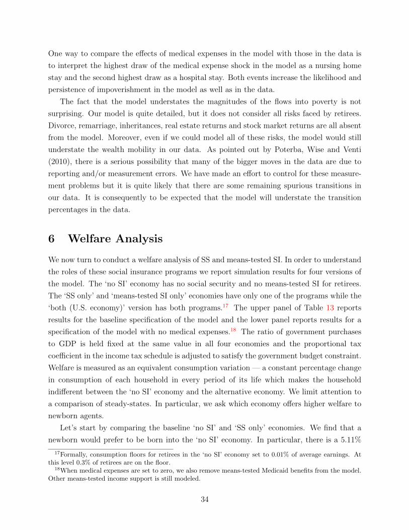
6 Welfare Analysis
We now turn to conduct a welfare analysis of SS and means-tested SI. In order to understand
the roles of these social insurance programs we report simulation results for four versions of
the model. The ‘no SI’ economy has no social security and no means-tested SI for retirees.
The ‘SS only’ and ‘means-tested SI only’ economies have only one of the programs while the
‘both (U.S. economy)’ version has both programs.17 The upper panel of Table 13 reports
results for the baseline specification of the model and the lower panel reports results for a
specification of the model with no medical expenses.18 The ratio of government purchases
to GDP is held fixed at the same value in all four economies and the proportional tax
coefficient in the income tax schedule is adjusted to satisfy the government budget constraint.
Welfare is measured as an equivalent consumption variation — a constant percentage change
in consumption of each household in every period of its life which makes the household
indifferent between the ‘no SI’ economy and the alternative economy. We limit attention to
a comparison of steady-states. In particular, we ask which economy offers higher welfare to
newborn agents.
Let’s start by comparing the baseline ‘no SI’ and ‘SS only’ economies. We find that a
newborn would prefer to be born into the ‘no SI’ economy. In particular, there is a 5.11%
17Formally, consumption floors for retirees in the ‘no SI’ economy set to 0.01% of average earnings. Atthis level 0.3% of retirees are on the floor.
18When medical expenses are set to zero, we also remove means-tested Medicaid benefits from the model.Other means-tested income support is still modeled.
34
Table 13: Aggregate variables for four economies: ‘baseline’ and the ‘no medical expense’specifications
Results are reported for four economies and two specifications of the model. The first column isthe ‘No SI’ economy in which there is no social security and no means-tested welfare for retirees.The second column is the ‘SS Only’ economy which has only social security. The third column isthe ‘Means-tested SI only’ economy which has only means-tested SI. The last column, ‘Both (U.S.Economy)’, has both programs. The ‘baseline’ specification includes medical expenses and the ‘nomedical expense’ specification sets medical expenses to zero. All flows are annualized. The measureof output in this table is GNP. Welfare is measured as an equivalent consumption variation — aconstant percentage change in consumption of each household in every period of its life that makesthe household indifferent between the ‘No SI’ economy and the alternative economy.
35
welfare loss of introducing SS. This is because the ‘no SI’ economy has more wealth and
higher consumption. SS distorts the savings decision and households save less. Interestingly,
average female hours worked by all women increases in the economy with SS. Underlying
this response are two countervailing effects.19 First, females increase participation so that
they can qualify for SS benefits. Second, a higher income tax is needed under SS to balance
the government budget constraint and this acts to depress hours per working female. The
participation effect is larger and average female hours worked by all women increases.
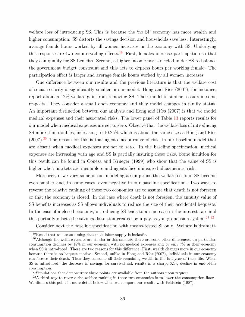
One difference between our results and the previous literature is that the welfare cost
of social security is significantly smaller in our model. Hong and Rıos (2007), for instance,
report about a 12% welfare gain from removing SS. Their model is similar to ours in some
respects. They consider a small open economy and they model changes in family status.
An important distinction between our analysis and Hong and Rıos (2007) is that we model
medical expenses and their associated risks. The lower panel of Table 13 reports results for
our model when medical expenses are set to zero. Observe that the welfare loss of introducing
SS more than doubles, increasing to 10.25% which is about the same size as Hong and Rıos
(2007).20 The reason for this is that agents face a range of risks in our baseline model that
are absent when medical expenses are set to zero. In the baseline specification, medical
expenses are increasing with age and SS is partially insuring these risks. Some intuition for
this result can be found in Conesa and Krueger (1999) who show that the value of SS is
higher when markets are incomplete and agents face uninsured idiosyncratic risk.
Moreover, if we vary some of our modeling assumptions the welfare costs of SS become
even smaller and, in some cases, even negative in our baseline specification. Two ways to
reverse the relative ranking of these two economies are to assume that death is not foreseen
or that the economy is closed. In the case where death is not foreseen, the annuity value of
SS benefits increases as SS allows individuals to reduce the size of their accidental bequests.
In the case of a closed economy, introducing SS leads to an increase in the interest rate and
this partially offsets the savings distortion created by a pay-as-you go pension system.21,22
Consider next the baseline specification with means-tested SI only. Welfare is dramati-
19Recall that we are assuming that male labor supply is inelastic.20Although the welfare results are similar in this scenario there are some other differences. In particular,
consumption declines by 18% in our economy with no medical expenses and by only 7% in their economywhen SS is introduced. There are two reasons for this difference. First, wealth changes more in our economybecause there is no bequest motive. Second, unlike in Hong and Rıos (2007), individuals in our economycan foresee their death. Thus they consume all their remaining wealth in the last year of their life. WhenSS is introduced, the decrease in savings for survival risk results in a sharp, 62%, decline in end-of-lifeconsumption.
21Simulations that demonstrate these points are available from the authors upon request.22A third way to reverse the welfare ranking in these two economies is to lower the consumption floors.
We discuss this point in more detail below when we compare our results with Feldstein (1987).
36
cally higher (14%) in this economy than in the ‘no SI’ economy. To understand this finding
one must balance the negative incentive effects of means-tested SI against its insurance ben-
efits. The negative incentive effects can be readily discerned in macroeconomic aggregates.
Introducing means-tested SI produces similar reductions in consumption and output as in-
troducing SS. In addition, both female participation and average hours of working women
decline. One of the negative incentive effects is due to higher taxes. The introduction of
means-tested SI requires government outlays amounting to 2.52% of GNP. This results in
higher income taxes and lower economic activity. The second negative incentive effect has
been emphasized by Feldstein (1987) and Hubbard et al. (1995). When means-tested SI is
available to retirees, poorer households will choose not to save for retirement. Instead they
consume all of their earnings while working and then roll directly onto means-tested SI at
retirement. In the ‘means-tested SI only’ economy this effect is very large and 21% of all
individuals start receiving means-tested benefits at age 65.
We find that the large magnitude of this second incentive effect is due to the presence
of old age medical expenses and their associated risks. When we set medical expenses to
zero, the fraction of households who start receiving means-tested benefits at age 65 falls to
5%. To understand this finding, note that there is more risk during retirement when medical
expenses are modeled. With means-tested SI agents must first use their own resources to
cover these expenses. What this means is that in some states of nature savings are subject
to implicit taxes of up to 100%. Poorer households are more likely to experience a high
implicit tax during retirement and thus have a lower expected return on savings. Their
optimal response is to not save for retirement.
In spite of these negative incentive effects the ‘means-tested SI only’ economy delivers the
highest welfare of all four economies and by a substantial margin. The single biggest reason
for this large difference in welfare is that this form of social insurance is an effective way to
insure against old age medical expense related risks. In contrast to SS benefits, means-tested
SI transfers pay out in situations where medical expenses are large and thus the need for
insurance is largest. Results in the lower panel illustrate this point. Notice that newborn
still like the ‘means-tested SI only’ economy best when medical expenses are zero. However,
the welfare gap between this economy and the economy with no SI is substantially smaller
and for some households such as those who are college educated the gap is close to zero.
Our results for the ‘no medical expense’ specification are related to research on Australia
by Tran and Woodland (2012). All public pensions are means-tested in Australia. Tran
and Woodland (2012) assess the welfare benefits of this system in a small open economy,
OLG model with earnings and survival risks. They find that the negative incentive effects
of this public pension system are so large that newborn agents prefer no public pension.
37
They go on to show that this result is sensitive. Modifying the rate at which benefits taper
off can produce welfare gains as compared to no program. Similarly, in our ’no medical
expense’ specification, one can come up with variants of the calibration that would overturn
our relative ranking of the ‘no SI’ and the ‘means-tested SI only’ economies. One way to
do this would be to raise the consumption floors guaranteed by means-tested SI. However,
the welfare benefits of means-tested SI are much larger once medical expenses and their
associated risks are taken into account.
More generally, our baseline result that welfare is much higher in the ‘means-tested SI
only’ economy as compared to any other economy is very robust to some of the other details
of the model. As long as medical expenses and associated risks are present, changes to the
model, including removing anticipated death, closing the economy, or holding taxes fixed
as is done in partial equilibrium analyses, do not overturn our result. Utility of newborn
is highest in the ‘means-tested SI only’ economy regardless of whether these changes in the
model are made individually or jointly.23
So far we have considered each program in isolation. We now turn to discuss the in-
teractions when both programs are present as is the case in the U.S. We have seen that
newborn like the ‘means-tested SI only’ economy best in spite of the fact that there are large
distortions on incentives. Adding SS to this economy alters these incentives. Recall that
for some households the availability of means-tested income and health expenditure support
at retirement has a particularly strong influence on their savings decision. They choose to
consume all of their income while working and then to rely on means-tested SI at retirement.
Introducing social security decreases the fraction of agents who pursue this strategy. These
effects are illustrated in Figure 4. This figure displays the decline in Medicaid take-up rates
by age for each male permanent earnings quintile when social security is introduced into the
‘means-tested SI only’ economy.24 The left panel shows results for the ’baseline’ specification
and the right panel displays the same information for the ’no medical expense’ specification.
In the baseline specification introducing social security has a very pronounced effect on
take-up rates. The fraction of households who choose to roll into SS at retirement falls by 15%
for permanent earnings quintile 1, 15% for quintile 2 and 18% for quintile 3. Interestingly,
there is no increase in take-up rates at retirement for those in quintiles 4 and 5. Note also
that the pattern of the additional Medicaid enrollment varies quite distinctly by age and
quintile. For those in quintiles 1 and 2, the decline in enrollment plummets early and then
increases with age. In quintile 3, the fall in enrollment continues until age 83. And for the
23Simulations that demonstrate this point are available from the authors upon request.24We wish to emphasize that male permanent earnings are distinct from household wealth or household
earnings. We use male permanent earnings because they are exogenous. This makes it possible to comparethe same individuals across economies.
38
6 5 7 0 7 5 8 0 8 5 9 0- 6 0
- 5 0
- 4 0
- 3 0
- 2 0
- 1 0
0
6 5 7 0 7 5 8 0 8 5 9 0- 6 0
- 5 0
- 4 0
- 3 0
- 2 0
- 1 0
0
Q 2Q 3
Q 4 , Q 5Q 4
Q 1
Q 3
Q 2
Q 5Pe
rcent
Chan
ge
A g e
Q 1
N o M e d i c a l E x p e n s e s
A g e
Perce
nt Ch
ange
B a s e l i n e
Figure 4: The percentage decrease in means-tested SI take-up rates of retirees when socialsecurity is introduced into the ‘means-tested SI only’ economy. The change in the take-uprates is shown by age and male permanent earnings quintile. The left panel is the baselinespecification and the right panel is the ‘no medical expense’ specification. The percentagedecrease is calculated by subtracting the take-up rates in the economy with means-tested SIonly from those in the economy with both means-tested SI and SS.
top two quintiles take-up rates are zero until very late in life.
The reason why introducing SS has such a dramatic impact on means-tested SI take-up
rates is because it ameliorates the negative saving effect of means-tested SI described above.
SS forces some households to save for retirement who would choose not to save otherwise.
This forced savings increases the expected return from private savings and some households
alter their strategy and choose to save on their own as well.
The effect of introducing SS on means-tested take-up rates is most pronounced when
medical expenses are present. This can be seen by comparing the left-hand and right-
hand panels of Figure 4. In the economy without medical expenses, when social security is
introduced, only 10% of those in the first quintile choose not to save but roll into means-
tested SI at retirement. Households in all other quintiles choose to save while working
in order to smooth consumption over their life-cycle when social security is introduced.
Another difference between the two panels is that in the right panel take-up rates decrease
monotonically with age for those in quintiles 1–3. It is clear from this figure, that when
medical risks are absent, the primary role played by means-tested income support is insurance
against survival risk.
Overall, introducing SS reduces means-tested SI take-up rates from 34% to 13%. As a
result, government expenditures on means-tested SI for retirees fall from 2.52% of GNP to
39
Table 14: Welfare effects of introducing social security into the ‘means-tested SI only’ econ-omy and the ‘no SI’ economy by household type
Economy Means-tested SI only No SIIncome Taxes Adjusted Fixed Adjusted Fixed
high school, high school -11.8 -9.49 -4.31 -1.72high school, college -11.1 -7.69 -6.68 -1.96college, high school -12.8 -9.68 -7.01 -2.68college, college -12.2 -8.16 -8.95 -2.69
Columns are the percentage change in welfare of introducing SS into the ‘means-tested SI only’and the ‘no SI’ economies. The first and third columns show the welfare change when incometaxes adjust to balance the government budget constraint. The second and fourth columns showthe welfare change when income taxes remain fixed at their value before SS is introduced. Welfarechanges are measured as equivalent consumption variations — the constant percentage change inconsumption of each household in every period of its life that makes the household indifferentbetween the reference economy and the reference economy with SS.
0.80% of GNP. Despite this, taxes go up in the economy with both programs. The negative
effect of SS on private savings that we discussed above are still significant and wealth is
lower in the economy with both programs as compared to the economy with means-test SI
only. Despite the large fiscal benefits we have described welfare of a newborn falls when this
program is introduced. Rich households like lower means-tested take-up rates because they
lower government outlays but the poor do not. Effectively forcing the poor to save lowers
their utility. These factors in conjunction with the low effective return of SS contributions
act to lower average welfare of newborn by 11.8%.
So far we have limited attention to average welfare of a newborn. Column one of Table 14
reports the change in welfare going from the ‘means-tested SI only’ economy to the economy
with both programs for different types of households. A comparison of welfare in these two
economies is of interest because the ‘means-tested SI only’ economy produces the highest
average welfare and the economy with both programs is our baseline model for the U.S.
40
Welfare changes are reported by education status of the female and male members of the
household. For purposes of comparison, we also report welfare organized by male permanent
earnings quintile. The results are very strong: welfare of all types of households is lower in
the economy with both programs as compared to the economy with means-tested SI only.
Table 14 has several other noteworthy properties that can be seen by considering the
second column, which holds income taxes fixed at their levels in the ‘means-tested SI only’
economy. This corresponds to the type of situation considered in partial equilibrium studies.
Observe that holding taxes fixed understates the total welfare loss of introducing SS. As we
noted above, introducing SS has two fiscal effects: it reduces means-tested SI take-up rates;
and it distorts the saving decision of more affluent households. This latter effect is dominant
and taxes go up when they are allowed to adjust and welfare of all types falls.
The treatment of taxes also affects the pattern of welfare losses. When taxes are held
fixed, the welfare losses increase with permanent earnings, but when taxes are allowed to
adjust, this pattern is reversed. With taxes fixed the poor are particularly unhappy about
the introduction of SS. This program prevents them from running down their wealth and
reduces their ability to qualify for means-tested SI when retired. The rich, in contrast,
dislike SS less since they do not have to pay for it. Once taxes adjust though, the rich are
particularly, unhappy. They are subject to a disproportionate share of the tax burden due to
the tapering in U.S. SS benefit formulas (replacement rates fall as indexed earnings increase,
as reported in Section 8.3.6).
Finally, note that households with college educated males dislike SS less than households
with high-school educated males. The reason for this asymmetry is that SS provides spousal
and survivor benefits that are particularly attractive to households with college educated
males.
The final two columns of Table 14 report results that are designed to understand welfare
of the poor when SS is introduced into an economy with very small means-tested SI. Feldstein
(1987) has previously argued that the poor will prefer SS to means-tested SI if means-tested
SI support levels are sufficiently low. Moreover, he asserts that the benefits for the poor of
introducing SS could be so large as to dominate the welfare losses for other households. We
evaluate these claims by considering the welfare effects of moving from the ’no SI’ economy
to the economy with SS only. Recall that in our ‘no SI’ economy consumption floors of
retirees are set at 0.1% of average earnings or about $48 per year using year 2000 prices.
Introducing SS into the ‘no SI’ economy thus provides us with a way to see whether poor
benefit from SS when consumption floors are set to a very low level. Table 14 shows that
regardless of whether taxes are held fixed or allowed to adjust, quintile 1 households prefer to
be born into the economy with no SS. Even this very low setting of the consumption floor is
41
Table 15: Welfare and fiscal effects of changes in the means-tested SI consumption floor
Means-tested SI floorsNo change
30% up 30% up 30% downTax Adjusting Income Payroll Income
WelfareAverage 0.0 -0.44 0.54 0.04
By household education type (female, male):
high school, high school 0.0 -0.24 0.62 -0.13high school, college 0.0 -0.91 0.35 0.45college, high school 0.0 -0.69 0.48 0.28college, college 0.0 -1.20 0.29 0.65
The first column is the ‘both (U.S. economy)’ version under the baseline specification. The secondcolumn shows the welfare and fiscal effects of increasing the means-tested SI floor by 30% financedby an an increase in income taxes. The third column shows the effect if the increase is financedby payroll taxes instead. The final column shows the effect if the floor is instead reduced by 30%and income taxes are adjusted. Welfare is measured as an equivalent consumption variation —a constant percentage change in consumption of each household in every period of its life whichmakes the household indifferent between the ‘both (U.S. economy)’ version and the alternativeeconomy with a different consumption floor.
too large to be consistent with Feldstein’s assertions. We have experimented with even lower
consumption floors and found that if the consumption floor is set at $4.8 instead, welfare of
the poor and average welfare of the newborn are both higher when SS is introduced to the
‘no SI’ economy. Medical expense and associated risks play an essential role in confirming
Feldstein’s assertions. In particular, if medical expenses are zero, average utility of a newborn
is higher in the economy with no SS. Even though it is possible to produce examples where
means-tested SI is so low that agents prefer SS, these cases are not relevant for the U.S. As
we have shown, as long as means-tested SI remains close to levels currently available, all
newborn strongly prefer the economy with means-tested SI only over all other economies we
have considered.
6.1 Reforming Social Insurance for Retirees
We have found that the long-run welfare benefits of shutting down SS and moving to a
single means-tested SI system for retirees are very large. It is clear though that the costs
of compensating retirees who loose SS benefits could offset some of these long-run welfare
42
gains. Assessing whether the U.S. should transition to a means-tested only SI system is
beyond the scope of this paper. Instead we focus on reforms of means-tested SI holding SS
fixed at its current level. We will provide an example where all types of newborn benefit
from increasing the current scale of means-tested SI for retirees in the U.S. In this example,
the costs of transition are not an issue. Current retirees benefit immediately from enhanced
retirement benefits and working households enjoy the same enhanced benefits when they
retire.
The central factor that determines the signs of the welfare effects of increasing means-
tested SI is how these additional benefits are financed. We find that welfare of all newborn
increases if the expansion of means-tested SI is financed with a payroll tax, but that all
newborn prefer the status quo if the income tax is used instead. These points are illustrated
in columns two and three of Table 15, which reports welfare changes associated with mov-
ing from the economy with both programs to an economy in which consumption floors for
retirees are 30% higher. Results are reported for average utility of a newborn and utility
by educational type. When means-tested SI expansion is financed by a payroll tax, average
welfare of a newborn increases by 0.54%. More importantly, all education types are better
off. Since educational status is the only source of initial heterogeneity, these results imply
that all newborn would prefer to be born into the economy with higher means-tested ben-
efits and higher payroll taxes even after they know their educational type. In contrast, if
the expansion is financed by a higher income tax, average welfare of a newborn declines by
0.44% and all newborn are worse off.
The reasons for this difference are that the payroll tax only applies to labor income
and is proportional, while the income tax applies to both labor and capital income and is
progressive. As a result an expansion of means-tested SI financed by the income tax leads
to a larger reduction in savings and a greater increase in SI take-up rates.
Our finding that households don’t want to increase means-tested SI if it is financed with
a higher income tax raises the question of whether they would prefer a smaller means-tested
SI program and lower income taxes. The final column of Table 15 shows that average utility
is in fact marginally (0.04%) higher when consumption floors are reduced by 30%. However,
there is a disagreement among newborn. Households with two high school educated members
are worse off. However, this loss is smaller than the combined gain of other types of newborn.
6.2 Robustness
Before concluding we briefly discuss the robustness of our results to several simplifying as-
sumptions we have made. Probably the most important question concerning our assumptions
43
pertains to medical expenses and their associated risks. We have found that these risks play
a central role in our welfare analysis and the question that arises is how robust are our con-
clusions to our assumptions about the availability of alternative forms of insurance against
these risks.
First, our conclusions are premised on a model that abstracts from private insurance
markets. It is doubtless the case that if these markets were modeled and no SI was available
demand for products such as life insurance and long-term care insurance would increase.
However, it is our view that the increase in take-up rates in these markets would be small.
Hendren (2013) finds that rejection rates in these insurance markets are high. He argues
that an important reason for this is asymmetric information. Namely, individuals have
superior information about their health status as compared to issuers and this information
is significant in the sense that it can have a very large impact on payouts and thus pricing.
Adverse selection limits the functioning of these markets in several ways. Insurers deny
coverage to individuals who have observable characteristics that predispose them to these
risks. Other individuals who know they have low risk will choose not to purchase insurance.
Moreover, some poor individuals will not be able to afford private insurance even if they
want it. Absent a government mandate or other types of regulation it is likely that many
individuals will end up old, sick alone, poor and uninsured.
Second, Medicare also provides insurance against old-age medical risks. We model the
component of the payroll tax that is used to finance Medicare and retirees OOP medical
expenses are net of Medicare benefits. However, we are not able to explicitly link Medicare
tax contributions to Medicare benefits because our HRS data does not include pre-Medicare
medical expenses. Consequently, it is difficult to consider experiments that assess the welfare
benefits of Medicare. Still, our current results do shed some light on how agents would assess
a change in the scale of Medicare. Medicare is a universal pay-as-you-go public healthcare
program and has the same incentive effects on savings as SS. We thus conjecture that, if
the scale of Medicare were reduced in our model where medical expenditures are exogenous,
newborn households would also experience welfare gains.
A final type of insurance of medical risks for retirees is Medigap, a government regulated
private insurance market that covers copayments, deductibles and other OOP expenses for
Medicare insured risks. Medigap provides no coverage for long-term care expenses which is
the biggest source of medical risk for retirees (see Kopecky and Koreshkova (2007)).
We have found that the welfare benefits of means-tested SI are large. Are we overstating
them? If anything, our estimates may be too conservative because we have assumed that
medical expenses are not growing. Since 1980 health-expenditures as a fraction of GDP
44
have doubled.25 If we were to model this observation the welfare benefits of means-tested SI
would be even larger.
In this paper we have focused on the welfare effects of changes in the scale of SS and
means-tested SI. We have not considered alternative arrangements that might be better.
The large welfare gains of removing SS in our model are driven by the fact that the effective
return on SS contributions is very low. This has led others such as Prescott and McGrattan
(2012) to propose defined contribution public pension plans instead. In our model, poorer
households will not like this program because it forces them to save more, reducing their
ability to rely on means-tested SI during retirement. However, wealthier households will like
this program. They plan to save anyway and the return on their defined contributions will
be close to the return on their private savings. Moreover, by forcing the poor to save, the
program decreases government outlays for means-tested SI and thus taxes to finance them.
Given the opposing impact of such a program on the welfare of the rich versus the poor, it is
unclear whether average welfare would increase of fall if this type of pension program were
implemented. However, work by Golosov and Tsyvinski (2006) suggests that even if such a
program was offered that there would still be a Pareto enhancing role for means-tested SI.
7 Conclusion
One of the central objectives of public policy is to provide for those who are sick and do
not have the financial means to cover their medical and living expenses. For the aged,
this risk is significant and can be compounded by a spousal death event leaving the retiree
not only sick and alone but also poor. We have shown that modeling these factors has a
very large impact on the relative welfare benefits of two social insurance (SI) programs that
help retirees cope with these risks: means-tested SI and Social Security (SS). We find the
following. First, given the choice of either no SI programs, a SS program only or a means-
tested SI program only, all newborn individuals strongly prefer the means-tested SI program
only to no SI programs and all newborn prefer no SI programs at all to having only a SS
program. Second, when means-tested SI is available, there is a large welfare loss associated
with the additional presence of SS. In other words, Friedman’s suggestion to get rid of SS is
good policy in our setting: means-tested SI is enough. Third, given the presence of SS, the
current scale of means-tested SI for retirees is about right.
25See OECD Health Data.
45
8 Appendix
8.1 Our HRS sample
The principal data set used in this paper the 1995–2010 waves of HRS and AHEAD and
includes retired individuals aged 65 and above who are single or married to retired spouses.
Our sample is essentially the same as that of Kopecky and Koreshkova (2007) and we refer
the interested reader to that paper for more specifics on the construction of the sample. We
define healthy individuals to be those who self-report their health status to be excellent, very
good or good.
8.1.1 Wealth Transitions
We use the wealth variable (ATOTN) which is reported at the household level in the HRS.
This wealth measure is the sum of the value of owned real estate (excluding primary resi-
All these values are taken from Heathcote et al. (2010).
Following Heathcote et al. ( 2010), we assume that females and males face a persistent
productivity shock process. In particular, εie is assumed to follow an AR(1) process with a
serial correlation coefficient of εie = 0.973 and a standard deviation of 0.01. We allow the
innovation to earning productivity to be correlated with the spouse’s innovation. Heathcote
51
et al. (2010) choose this correlation to reproduce a targeted correlation of male wage growth
and female wage growth of 0.15. We set the correlation of the earnings innovations to match
this same target. The resulting correlation between the two earnings innovations is 0.05.
Heathcote et al. (2010) also allow for a transient shock to labor productivity. We abstract
from this second shock. This reduces the size of the state space for working households and
allows us to model the problem of retirees in more detail.
The distribution of initial productivity levels Γe is assumed to be bivariate normal with
a standard deviation of 0.352, a correlation of 0.517 and a gender productivity gap of 0.62
in 1970. All of these targets are taken from Heathcote et al. (2010) and apply to males and
females.27
One difference between us and Heathcote et al. (2010) is that we allow for an earnings
state that has a much lower level of earnings as compared to what Gaussian quadrature
methods would imply. This is done to deal with the fact that some households receive very
little social security income during their retirement. The resulting process is non-Gaussian.
In order to recover to make this process consistent with the estimates of Heathcote et al.
(2010), we use the same simulated method of moments strategy described above for the
medical expense process.
8.3.5 Progressive Income Tax Formula
The effective progressive income tax formula is given by:
τ y(ydisp, d) =[ηd1 + ηd2 log
(ydispy
)]ydisp (19)
where ydisp is disposable household income, y is mean income in the economy. Guner et al.
(2012) estimate η01 = 0.113 and η02 = 0.073 for married households and ηd∈1,21 = 0.153 and
ηd∈1,22 = 0.057 for single households.
The U.S. Federal tax code allows tax-filers a deduction for medical expenses that exceed
7.5% of income. Our income tax schedules indirectly account for deductions when estimating
effective tax functions. However, their effective tax functions are averages across many
households and do not capture the full benefit of this deduction to those who experience
large medical expenditure shocks such as long-term care. We allow for a deduction for
medical expenses that exceed 7.5% of income.
U.S. Federal tax code provides for an exemption of SS benefits. This exemption is phased
out in two stages as income rises. Table 16 reports exemption thresholds and minimum
27Specifications similar to this have been used by Attansio et al. (2008) and Heathcote et al. (2008) tomodel the joint earnings of married couples.
52
Table 16: Exemption thresholds and minimum income levels for taxation of social securitybenefit income
Description Levels ($) % of ave. earnings
Threshold 1Single (T 1
s ) 25,000 53Married (T 1
m) 32,000 67
Threshold 2Single (T 2
s ) 34,000 72Married (T 2
m) 44,000 93
Minimum incomesingle (Y s) 4,500 9married (Y m) 6,000 13
Source: Scott, C. and J. Mulvey (2010). “Social Security: Calculation and Historyof Taxing Benefits”, Congressional Research Service.
income levels by marital status. The left column of Table 16 reports the actual dollar
amounts in the year 2000. The right column expresses these figures as a fraction of average
earnings of full-time, prime-age male workers in 2000 which according to SSA was $47, 552.16.
According to our source, the thresholds and minimum income are not indexed to inflation
or wage growth.
We use these thresholds to compute the exemptions formulas in the following way. We
start by calculating provisional income, Y , which is defined as asset income,Y a, plus half
of the household’s SS income, Y ss. If Y < T 1i , i ∈ s,m, there is a full exemption for SS
benefits and taxable income for that household is equal to Y a net of the medical expense
tax deduction. If T 1i < Y < T 2
i , i ∈ s,m, taxable income is given by
Y a + 0.5 min(Y ss, Y − T 1i ),
net of the medical expense tax deduction if eligible. If Y > T 2i , i ∈ s,m, then taxable
income is given by
Y a + min
0.85Y ss, 0.85[Y − T 2
i + min(Y i, 0.5Yssi )],
net of medical expense tax deduction if eligible.
53
8.3.6 Social Security Benefits
The U.S. Social Security system links a worker’s benefits to an index of the worker’s average
earnings, e. Benefits are adjusted to reflect the annual cap on contributions and there is also
some progressivity built into the U.S. Social Security system. We use the following formula
to link contributions to benefits for an individual
S(e) =
s1e, for e ≤ τ1,
s1τ1 + s2(e− τ1), for τ1 ≤ e ≤ τ2,
s1τ1 + s2(τ2 − τ1) + s3(e− τ2), for τ2 ≤ e ≤ τ3,
s1τ1 + s2(τ2 − τ1) + s3(τ3 − τ2), for e ≥ τ3.
Following the Social Security administration, we set the marginal replacement rates, s1, s2,
and s3 to 0.90, 0.33, and 0.15, respectively. The threshold levels, τ1, τ2, and τ3, are set to
20%, 125% and 246% of average earnings for all workers. The U.S. Social Security system
also provides spousal and survivor benefits. We model these benefits. Household benefits
are determined using the following formula
S(e, d) =
S
(maxi∈m,f
ei)
+ max
0.5S
(maxi∈m,f
ei), S
(min
i∈m,fei
), if d = 0,
maxS (em) , S
(ef) . if d ∈ 1, 2.
54
References
[1] Attanasio A., H. Low and V. Sanchez-Marcos, (2008). “Explaining Changes in FemaleLabor Supply in a Life-Cycle Model,” American Economic Review, Vol. 98 no. 4, pp:1517–52.
[2] Auerbach, A. and L.J. Kotlikoff, (1987) Dynamic Fiscal Policy Cambridge UniversityPress.
[3] Brown, J. and A. Finkelstein (2008). “The Interaction of Public and Private Insurance:Medicaid and the Long-Term Care Insurance Market.” American Economic Review, vol.98, no. 3, pp: 1083–1102.
[4] Castaneda, A., J. Diaz-Gimenez, J.V. Rıos-Rull (2003). “Accounting for the U.S. Earn-ings and Wealth Inequality,” Journal of Political Economy, vol. 111, no. 4, pp: 818–857.
[5] Cohen, W. J. and M. Friedman (1972). “Social Security: Universal or Selective.” Amer-ican Enterprise Institute for Public Policy Research.
[6] Conesa J. C., and D. Krueger (1999). “Social Security Reform with HeterogeneousAgents.” Review of Economic Dynamics, Vol. 2, no. 4, pp: 757–795.
[7] De Nardi, M., E. French, J. B. Jones (2010). “Why Do the Elderly Save? The Role ofMedical Expenses,” Journal of Political Economy, Vol. 118, no. 1, pp: 39–75.
[8] De Nardi, M., E. French, J. B. Jones (2012). “Medicaid insurance in old age,” WorkingPaper WP-2012-13, Federal Reserve Bank of Chicago.
[9] Erosa, A., L. Fuster and G. Kambourov (2012). “Labor supply and government pro-grams: A cross-country analysis,” Journal of Monetary Economics, Vol. 59 no. 1, pp:84–107.
[10] Feenberg, D. and J. Skinner, (1994) “The Risk and Duration of Catastrophic HealthCare Expenditures.” The Review of Economics and Statistics vol. 76, no. 4, pp: 633–647.
[11] Feldstein, M. (1987). “Should Social Security Be Means Tested?” Journal of PoliticalEconomy, vol. 95, no. 3. pp: 468–484.
[12] French, E., and J. B. Jones (2004). “On the Distribution and Dynamics of Health CareCosts,” Journal of Applied Econometrics, vol. 19, no. 4, pp: 705–721.
[13] Fuster, L., A. Imrohoroglu and S. Imrohoroglu (2007). “Elimination of Social Securityin a Dynastic Framework,” forthcoming, Review of Economic Studies, vol. 74, no. 1,pp: 113–145.
[14] Golosov, M. and A. Tsyvinski, (2006) “Designing Optimal Disability Insurance: A Casefor Asset Testing.” Journal of Political Economy vol. 114, no. 2, pp: 257–279.
55
[15] Gomme, P. and P. Rupert (2007). “Theory, Measurement and Calibration of Macroe-conomic Models,” Journal of Monetary Economics, vol. 54, no. 2, pp: 460–497.
[16] Guner, N., R. Kaygusuz and G. Ventura (2012) “Taxing Women: A MacroeconomicAnalysis.” Journal of Monetary Economics, vol. 59, no. 5, pp: 111–128.
[17] Heathcote J., K. Storesletten and G. L. Violante (2010). “The Macroeconomic Implica-tions of Rising Wage Inequality in the United States,” Journal of Political Economy,Vol. 118 no. 4, pp: 681–722.
[18] Hong, J. H. an J-V. Rıos-Rull (2007). “Social security, life insurance and annuities forfamilies,” Journal of Monetary Economics, Vol. 54, no. 1, pp: 118–140.
[19] Hoover, D.R., S. Crystal, R. Kumar, U. Sambamoorthi and J.C. Cantor (2002) “MedicalExpenditures during the Last Year of Life: Findings from the 1992-1996 MedicareCurrent Beneficiary Survey,” Health Services Research, Vol. 37 no. 6 pp: 1625-1642.
[20] Hubbard, G.R., J. Skinner, and S. Zeldes (1995). “Precautionary Savings and SocialInsurance,” Journal of Political Economy, vol. 103, no. 2, pp: 360–399.
[21] Keane, M. and R. Rogerson (2012). “Micro and Macro Labor Supply Elasticities: AReassessment of Conventional Wisdom,” Journal of Economic Literature Vol 50 no. 2,pp: 464–76.
[22] Kopecky, K. and T. Koreshkova (2007). “The Impact of Medical and Nursing HomeExpenses and Social Insurance Policies on Savings and Inequality,” unpublishedmanuscript.
[23] Kaygusuz, R. (2010). “Taxes and Female Labor Supply,” Review of Economic Dynamics,Vol. 13, no. 4, pp: 725–741.
[24] Liu, K. T. McBride and T. Coughlin (1994) “Risk of Entering Nursing Homes for Longversus Short Stays,” Medical Care, Vol 32, no. 4 pp: 315–327.
[25] McGrattan E. R. and R. Rogerson (2007). “Changes in the distribution of family hoursworked since 1950,” Staff Report 397, Federal Reserve Bank of Minneapolis.
[26] McGrattan E. R. and E. C. Prescott (2012) “On Financing Retirement with an AgingPopulation.” Staff Report 472, Federal Reserve Bank of Minneapolis
[27] Murtaugh, C. M., P. Kemper, B.C. Spillman and B. Lepidus Carlson (1997) “TheAmount, Distribution, and Timing of Lifetime Nursing Home Use,” Medical Care, Vol.35 no. 3, pp: 204–218.
[28] Nishiyama, S. and K. Smetters (2007). “Does Social Security Privatization ProduceEfficiency Gains?” The Quarterly Journal of Economics, vol. 122, no. 4, pp: 1677–1719.
56
[29] Poterba, J.M., S. F. Venti and D. A. Wise, (2011). “Family Status Transitions, LatentHealth, and the Post-Retirement Evolution of Assets,” in ed. D. Wise, “Explorations inthe Economics of Aging,” University of Chicago Press.
[30] Sefton, J., J. van de Ven and M. Weale, (2008) “Means Testing Retirement Benefits:Fostering Equity or Discouraging Savings?” The Economic Journal vol. 118, pp: 556–590.
[31] Storesletten, K., C. Telmer, and A. Yaron (2004). “Consumption and Risk Sharing Overthe Life Cycle,” Journal of Monetary Economics, vol. 51, pp: 609–633.
[32] Tran, C. and A. Woodland (2012). “Trade-Offs in Means Tested Pension Design,” Un-published Manuscript.