OLIGOPOLY. The Simplest Model of Price Competition in a Duopoly: The Bertrand Model. The Symmetric Bertrand Model in a Homogenous Good Market. Two identical firms: 1, 2. Identical product. Constant Returns to Scale: Unit cost of production = c (for both firms). Market demand curve: D(p) downward sloping, smooth.
Transcript
OLIGOPOLY.
The Simplest Model of Price Competition in a Duopoly:The Bertrand Model.
The Symmetric Bertrand Model in a Homogenous GoodMarket.
Two identical firms: 1, 2.
Identical product.
Constant Returns to Scale: Unit cost of production = c(for both firms).
Game: Firms set their prices p1, p2 simultaneously.
The quantity sold by each firm depends on both prices.
In particular, if p1 < p2, then firm 1 sells the entiremarket demand D(p1) while firm 2 sells zero.
The reverse happens when p1 > p2.
If p1 = p2 = p(say), then each firm sells 12D(p).
Nash equilibrium: A pair of prices (bp1, bp2) such thatneither firm can do better by unilaterally deviating andcharging some other price.
There are several possibilities:
1. A pair of prices (bp1, bp2) where bp1 > bp2 > c.
In this situation firm 1 earns zero profit. Firm 1 wouldbe better off unilaterally deviating and charging a pricep1 just below bp2.That way, it (firm 1) would make strictly positive profit.
So this cannot be a NE.
2. A pair of prices (bp1, bp2) where bp2 > bp1 > c : ruledout similarly.
3. A pair of prices (bp1, bp2) where bp1 = bp2 = bp(say) > c
In this case firm 1 earns profit = 12D(bp)(bp− c)
If it unilaterally deviates a charge a price slightly below bp,its profit will be approximately (slightly below) D(bp)(bp−c), almost double of what it was getting.
So, this cannot be a NE.
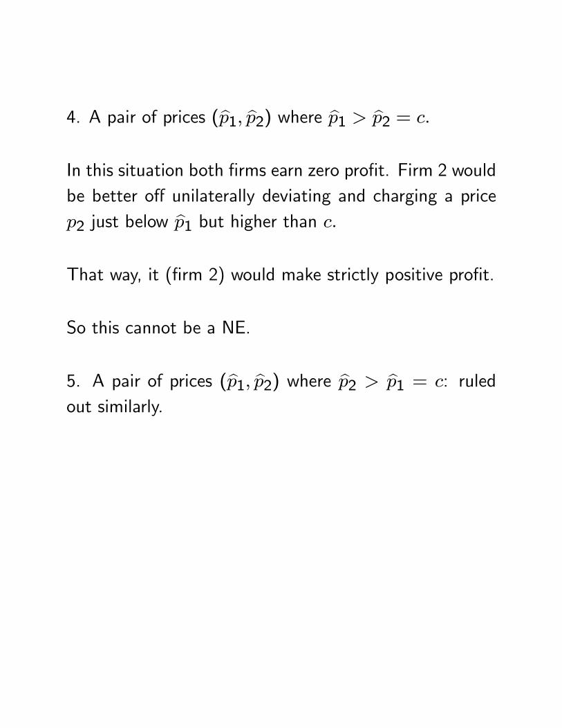
4. A pair of prices (bp1, bp2) where bp1 > bp2 = c.
In this situation both firms earn zero profit. Firm 2 wouldbe better off unilaterally deviating and charging a pricep2 just below bp1 but higher than c.That way, it (firm 2) would make strictly positive profit.
So this cannot be a NE.
5. A pair of prices (bp1, bp2) where bp2 > bp1 = c: ruledout similarly.
6. A pair of prices (bp1, bp2) where bp1 = bp2 = c.
In this case, both firms earn zero profit.
Further, no firm can deviate and do better i.e., strictlypositive profit.
This is a NE.
It is the unique NE.
If firms are identical, the unique NE is one where firmsset their prices = MC and the industry output is at thesocially optimal level.
Both firms earn zero profit.
Even with two firms - market power disappears.
If more than 2 firms - same outcome.
Bertrand paradox.
Assumptions of the Bertrand: rule out certain importantelements of real markets.
1. Product Differentiation:
In Betrand model, firms sell identical product
⇒firms can grab all buyers from rival by charging a slightlylower price (undercutting).
Real world: differentiated products
⇒ consumers may not switch to another firm simply be-cause it charges a lower price (care about difference inproduct attributes)
⇒ incentive for a firm to undercut rival’s price is muchless.
2. Dynamic competition:
Bertrand model is static (one shot game): prices chosenonly once.
Real world rival firms have long term interaction - repeat-edly choose prices over time.
Repeated games : better outcomes than in static games.
Possibility of future "retaliation" (through price war) candissuade firms from undercutting now.
3. Capacity Constraints:
Bertrand model: firms can produce as much as they wantat the same unit cost.
Real world: firms have limited production capacity.
Undercutting rival’s price to attract more buyers is notvery useful if the firm cannot produce more output tomeet the increased demand.
Consider a simple modification of the symmetric Bertrandduopoly model where each firm has a capacity constraint.
Let k1, k2 denote the capacity constraints of firms 1 and2.
A firm cannot sell more than its capacity.
Firms produce output at constant unit cost upto theircapacity.
For simplicity, set unit production cost= 0 for both firms.
Firms set prices simultaneously.
With capacity constraints, undercutting rival does notnecessarily reduce rival’s sales to zero; there may be apositive residual demand left for the rival.
For example, suppose p1 > p2.
Ideally, all consumers want to buy from firm 2.
IfD(p2) ≤ k2, then firm 2 sells the entire market demandD(p2) and firm 1 sells zero.
If, however,D(p2) > k2, then firm 2 sells k2which meansthere are consumers who want to buy from firm 2 but areturned away.
Some of them may be willing to buy from firm 1 at pricep1 > p2.
So, firm 1 can sell quantity D(p1)− k2
(or zero, if D(p1) < k2 which corresponds to a situationwhere none of the consumers turned away by firm 1 arewilling to pay the higher price).
In other words, for and price p1 > p2, the residual marketdemand curve facing firm 1 isD(p1)−k2 i.e., a horizontalleft-ward shift of the market demand curve by an amountof k2.
Consider a situation where the total industry capacityk1 + k2 is "small" relative to market demand.
Let p be the price at which market demand is exactlyequal to k1 + k2
D(p) = k1 + k2
What are the NE prices?
If k1 + k2 is small enough relative to market demand,NE: p1 = p2 = p.
Why?
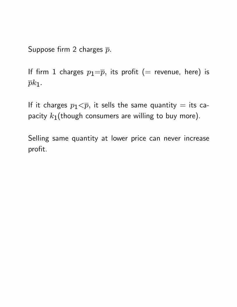
Suppose firm 2 charges p.
If firm 1 charges p1=p, its profit (= revenue, here) ispk1.
If it charges p1<p, it sells the same quantity = its ca-pacity k1(though consumers are willing to buy more).
Selling same quantity at lower price can never increaseprofit.
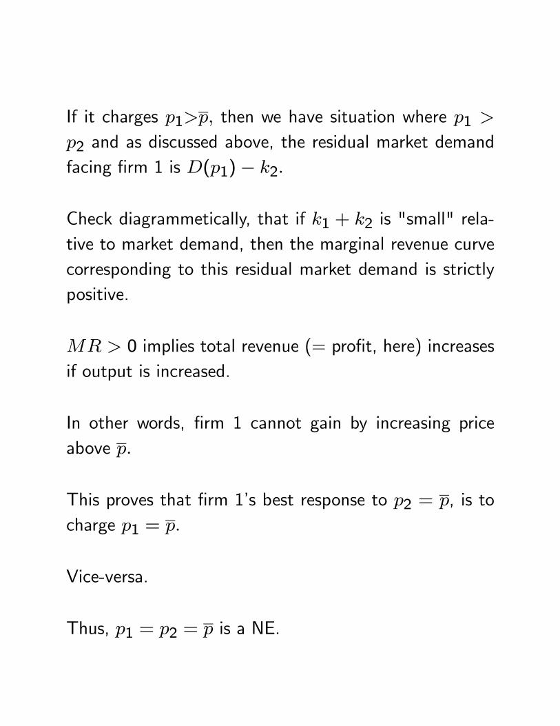
If it charges p1>p, then we have situation where p1 >p2 and as discussed above, the residual market demandfacing firm 1 is D(p1)− k2.
Check diagrammetically, that if k1 + k2 is "small" rela-tive to market demand, then the marginal revenue curvecorresponding to this residual market demand is strictlypositive.
MR > 0 implies total revenue (= profit, here) increasesif output is increased.
In other words, firm 1 cannot gain by increasing priceabove p.
This proves that firm 1’s best response to p2 = p, is tocharge p1 = p.
Vice-versa.
Thus, p1 = p2 = p is a NE.
Note that if k1+k2 is small, p is large and so firms havea lot of market power (price is considerably higher thanMC = 0).
Firms 1 and 2 make profit equal to k1p and k2p respec-tively.
What if k1 + k2 is large relative to market demand?
If firms split the market by charging equal prices, theircapacity is not fully utilized.
So, each firm undercuts rival to gain consumers.
Get back the Bertrand outcome.
Conclusion: More severe the capacity constraints, lesscompetitive the market and higher the extent of marketpower.
Industries with large capacity behave very competitively.
An Example of Price Competition with Capacity Con-straints.
Market Demand:
q = 100− p
The inverse demand
p = 100− q
There are two firms. Each with capacity constraint =20 (i.e., k1 = k2 = 20).
For simplicity assume that both firms have zero unit costof production.
Firms set prices simultaneously.
Claim: p1 = p2 = $60 is a Nash Equilibrium.
Note 60 is the price at which market demand is just suf-ficient to meet the industry output when both firms pro-duce at full capacity.
Why is this a NE?
Suppose firm 2 charges p2 = $60.
If firm 1 charges p1 = $60, the two firms split the marketequally and each firm sells 20 units leading to a profit of$1200 for the firm.
If firm 1 charges p1 < $60, it is the lower priced firm, itfaces demand of more than 40 units but can only sell 20units.
Its profit is 20p1 < $1200.
If firm 1 charges p1 > $60, it is the higher priced firm.
All consumers go to buy from firm 2 at price $60 & theirdemand is 40 units.
But firm 2 can only sell 20 units.
In order to figure out how many units will be bought fromfirm 1, we look at the residual market demand after 20units are sold by firm 2. This is given by
q = (100− p)− 20= 80− p
Firm 1 is like a monopolist facing this residualdemand.
From our discussion of elasticity of demand recall that fora straight line demand curve of this kind, price elasticity ofdemand is greater than 1 at all points above the midpoint(and MR > 0).
The midpoint of this (residual) demand curve (40, 40).
So definitely at any price above $60, demand is elastic.
This means firm can increase total revenue by reducingprice.
Therefore, raising p1above $60 cannot be more profitable(remember, here total revenue = profit).
Conclusion: p1 = $60 is a best response to p2 = $60.
Similarly, the converse holds true.
Therefore, p1 = p2 = $60 is a Nash Equilibrium.
Cournot Model of Quantity Competition.
Previous analysis: If production capacity is limited, thenfirms will set prices at a level such that the market de-mand exactly equals the total production capacity.
In the story so far: capacity is exogenously fixed.
But what levels of capacity will competing firms choose?
Higher the capacity, more intense the price competitionand smaller the price eventually charged in the market.
Need a model of endogenous capacity choice⇒ Cournot
oligopoly model.
In the Cournot model, firms choose their levels of output(or equivalently, their capacity to produce output) andit is assumed that the price at which they sell is one atwhich market demand equals industry output (or, indus-try capacity).
Simple Symmetric Cournot Duopoly Model:
Two identical firms, i = 1, 2.
Both firms produce at constant unit cost c ≥ 0.
Market demand: D(p)
Inverse demand: P (q)
Note P (q) gives us the demand price corresponding tototal quantity q.
Strategies of firms: output q1, q2.(interpret as capacity)
Industry output: q1 + q2
Then, the price in the "market" is P (q1 + q2)
Profit of firm 1 (its payoff):
π1(q1, q2) = q1P (q1 + q2)− cq1
Profit of firm 2 (its payoff):
π2(q1, q2) = q2P (q1 + q2)− cq2
Note that each firms’s profit depends on both its outputas well as its rival’s output (through the inverse marketdemand function that determines the price).
Other things being equal, if one firm increases its output,it reduces its rival’s profit because it reduces the price atwhich output is sold.
While a firm’s profit maximization process takes into ac-count the effect of its output on its own profit, it doesnot take into account the effect on rival’s profit.
This basic externality eventually hurts them both.
Nash equilibrium (NE): A pair of output (eq1, eq2) suchthat:
(i) given (belief about) firm 1’s output q1= eq1, firm 2maximizes its profit π2by choosing q2 = eq2(ii) given (belief about) firm 2’s output q2= eq2, firm 1maximizes its profit π1 by choosing q1 = eq1
In order to derive the NE, we first derive the optimal (orprofit maximizing) action of each firm for each possibleoutput of the rival firm.
This gives us the "best-response curve" or the "reactionfunction" of each firm.
By definition, a NE (eq1, eq2) is a point that lies on- the best-response curve for firm 1 because eq1 is firm 1’sbest response to eq2- the best-response curve for firm 2 because eq2 is firm 2’sbest response to eq1i.e., its the intersection of the two best response curvesor reaction functions.
Deriving the reaction function for firm 2:
Fix any output level q1 = q1 for firm 1.
Then, the residual demand faced by firm 2 is given by ahorizontal leftward shift of the market demand curve byan amount q1.
Firm 2 looks at the marginal revenue curve correspondingto this residual demand curve & equates it to the marginalcost c.
This determines the best response output of firm 2.
If q1 = 0, then the residual demand faced by firm 2is simple the market demand curve and so the point atwhich its MR equates MC is simply the monopoly outputqm.
So, the best response to zero output by rival, is to producemonopoly output.
For higher values of q1,the residual market demand islower, the corresoponding MR curve is even lower andthe point at which MR equates MC for firm 2 is smaller.
At q1 = qS, even if firm 2 produces zero, the marketprice is c (because market demand is equal to marginalcost c at qS) and so firm’s best response is zero.
So, in a graph where we measure the outputs of firms1 and 2 on the two axes, the reaction function of firm2 is a downward sloping curve whose intercept on theq2 − axis is the monopoly output qm and the intercepton the other axis is qS.
Note: qm < qS
Similarly, we can derive the reaction function of firm 1.
The point of intersection: NE.
Observe graphically that the point of intersection (eq1, eq2) :(i) lies above the straight line given by the equation q1+q2 = qm
(ii) lies below the straight line given by the equation q1+q2 = qS
Therefore,
qm < eq1 + eq2 < qS
This means that at the NE of the Cournot game, industryoutput lies between monopoly output and socially optimaloutput.
The price in the market at the NE outputs: P (eq1+ eq2) =ep(say).Then,
pm < ep < c
Deriving the NE of the Cournot model anlytically:
Consider the specific demand function:
q = 40− p
Suppose c = 10.
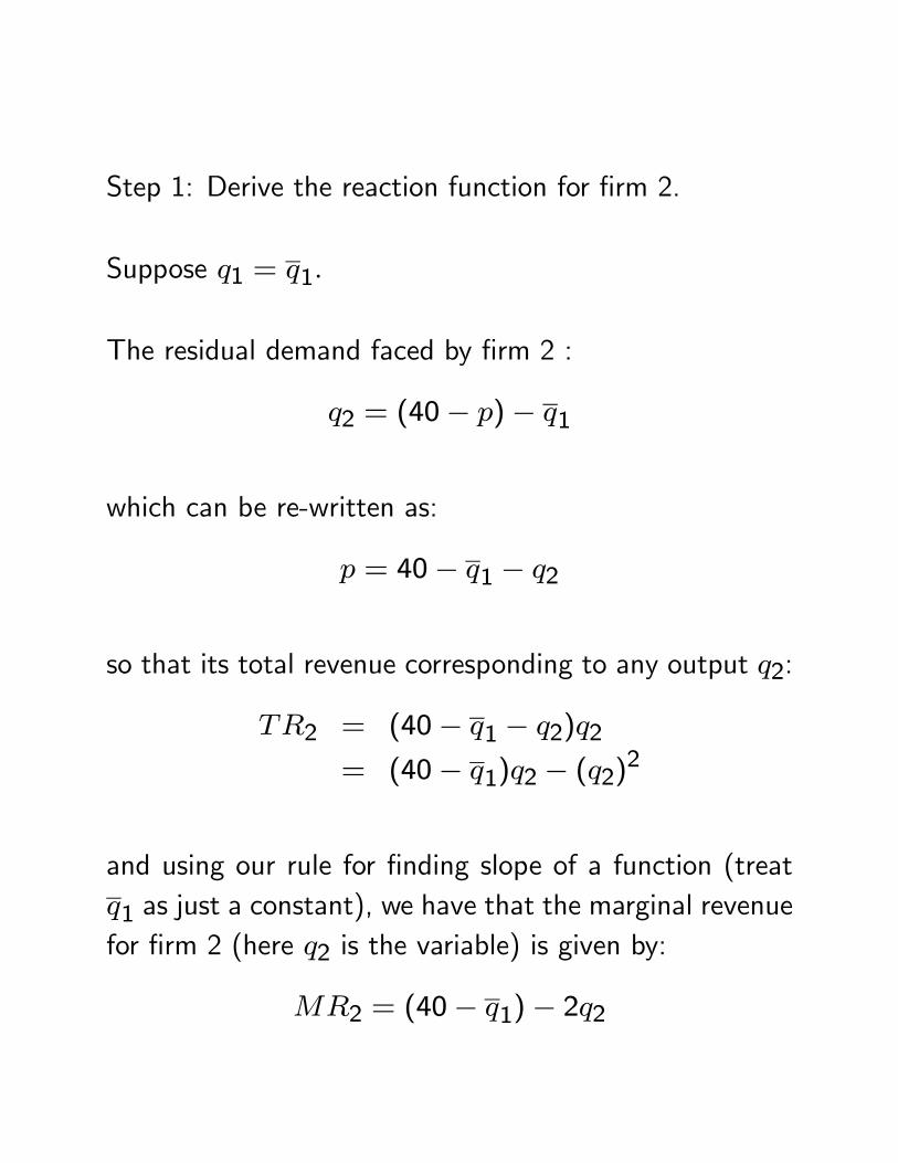
Step 1: Derive the reaction function for firm 2.
Suppose q1 = q1.
The residual demand faced by firm 2 :
q2 = (40− p)− q1
which can be re-written as:
p = 40− q1 − q2
so that its total revenue corresponding to any output q2:
TR2 = (40− q1 − q2)q2
= (40− q1)q2 − (q2)2
and using our rule for finding slope of a function (treatq1 as just a constant), we have that the marginal revenuefor firm 2 (here q2 is the variable) is given by:
MR2 = (40− q1)− 2q2
Putting MR2 =MC :
(40− q1)− 2q2 = 10
we have:
q2 = 15−q12
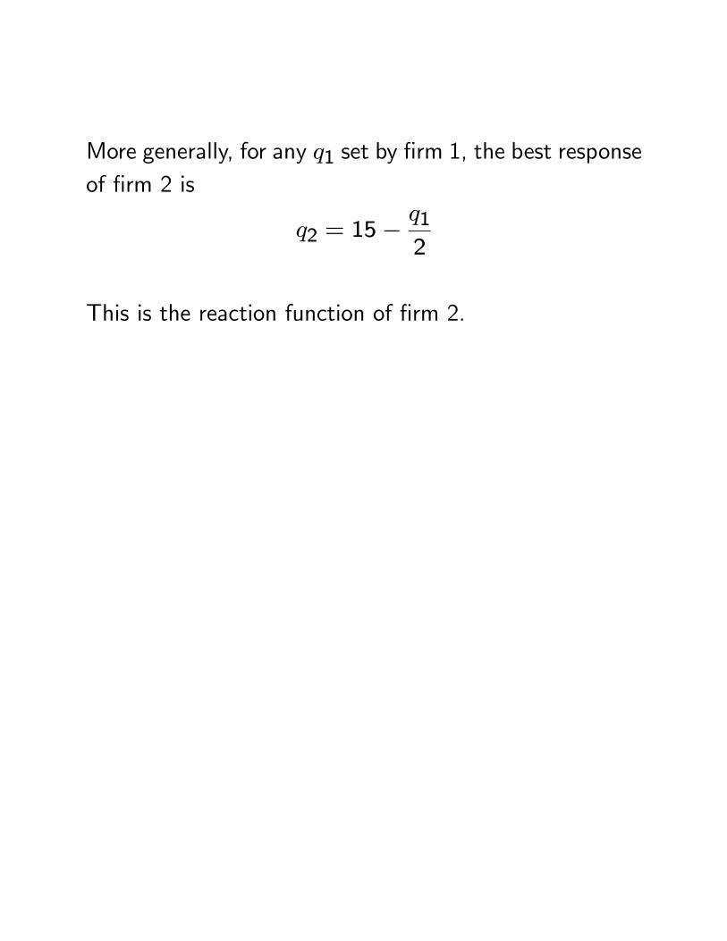
More generally, for any q1 set by firm 1, the best responseof firm 2 is
q2 = 15−q12
This is the reaction function of firm 2.
Step 2: Derive the reaction function for firm 1.
Suppose q2 = q2.
The residual demand faced by firm 1 :
q1 = (40− p)− q2
which can be re-written as:
p = 40− q2 − q1
so that its total revenue corresponding to any output q1:
TR1 = (40− q2 − q1)q1
= (40− q2)q1 − (q1)2
and using our rule for finding slope of a function (treatq2 as just a constant), we have that the marginal revenuefor firm 1 (here q1 is the variable) is given by:
MR1 = (40− q2)− 2q1
Putting MR1 =MC :
(40− q2)− 2q1 = 10
we have:
q1 = 15−q22
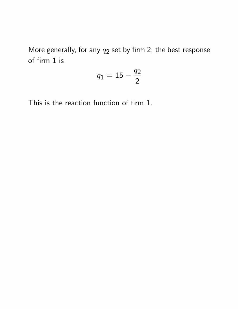
More generally, for any q2 set by firm 2, the best responseof firm 1 is
q1 = 15−q22
This is the reaction function of firm 1.
Step 3:
Find the point of intersection (eq1, eq2)of the two reactionfunctions.
Such a point must lie on both reaction functions i.e.,
eq1 = 15− eq22
eq2 = 15− eq12
Solve these two equations simultaneously for two un-knowns (eq1, eq2).Solution: eq1 = eq2 = 10.
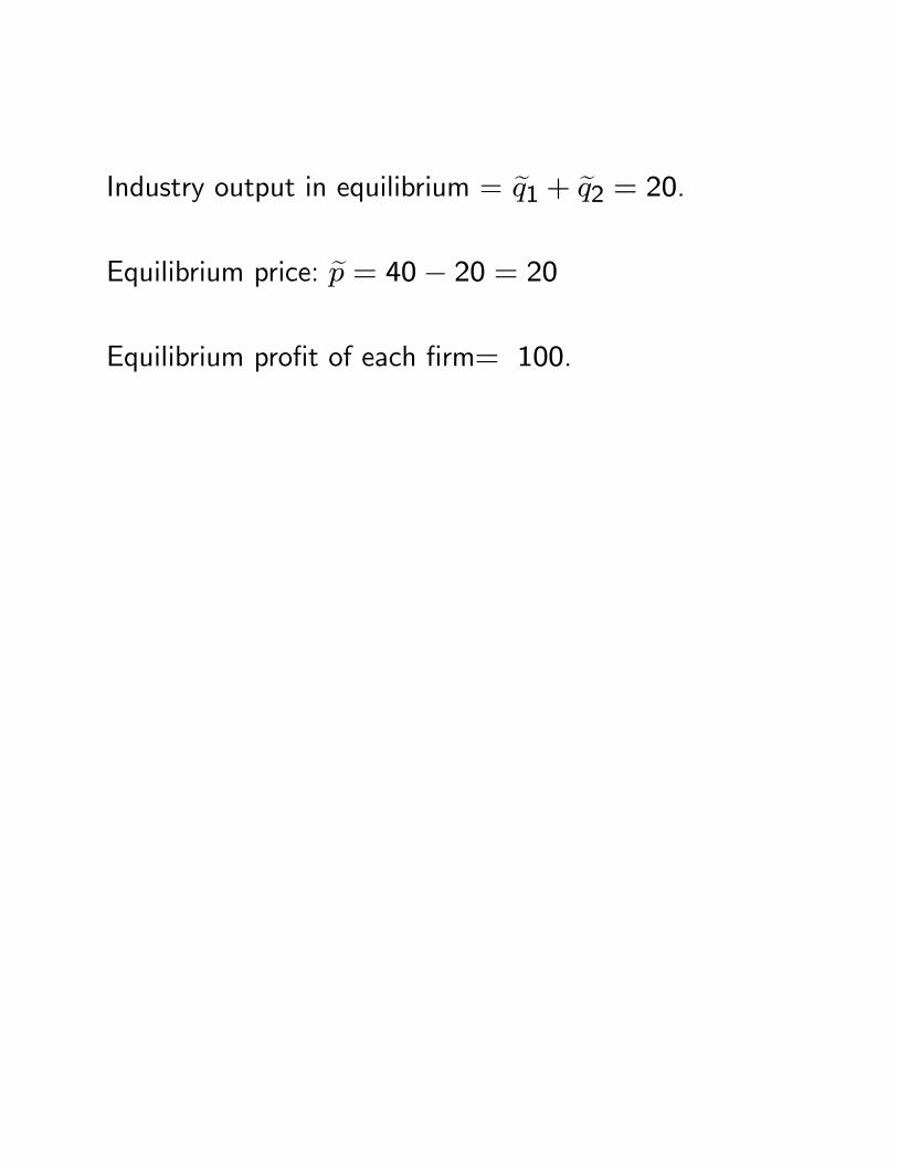
Industry output in equilibrium = eq1 + eq2 = 20.Equilibrium price: ep = 40− 20 = 20Equilibrium profit of each firm= 100.
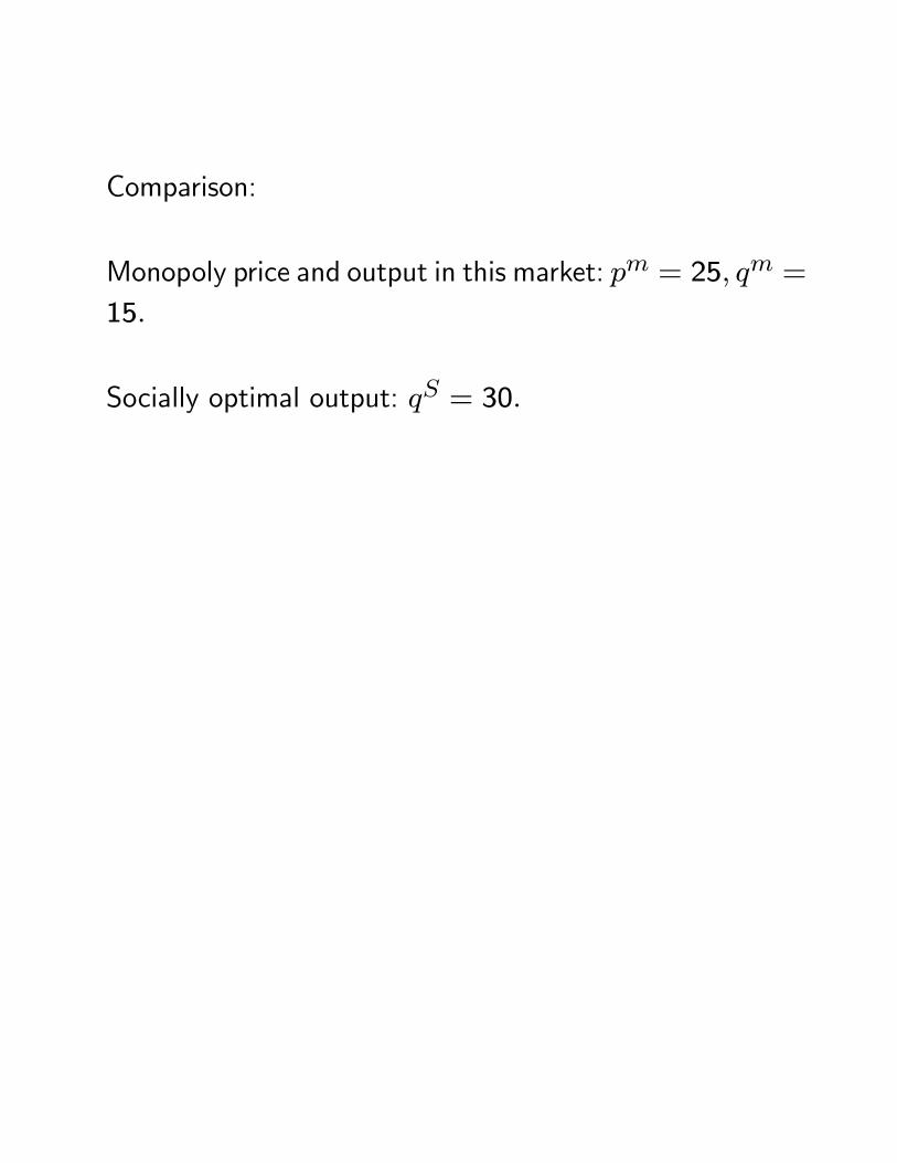
Comparison:
Monopoly price and output in this market: pm = 25, qm =
15.
Socially optimal output: qS = 30.
Asymmetric Cost Oligopoly.
In the models of oligopoly we looked at so far, firms areidentical.
What if firms differ in their efficiency or productivity?
Production costs may differ.
Bertrand Model with Asymmetric Cost.
2 firms: 1 and 2.
Both produce at constant unit cost.
Marginal cost of firm 1: c1
Marginal cost of firm 2: c2
Firms compete in prices - as in the standard model ofBertrand price competition (no capacity constraints).
We have seen that if c1 = c2, unique NE is that bothfirms set price equal to MC and earn zero profit.
What if c1 < c2?
First, note that firm 2 can never make money in any NE.
To make money, p2 > c2 in which case firm 1 will find itoptimal to undercut firm 2.
However, if firm 1 charges a price p1just below c2, it willnever be matched or undercut by firm 2 and it can makemoney.
This is actually the NE if c1 and c2 are not too far apart.
But if c2 is extremely high relative to c1 so that firm 1’smonopoly price is below c2, then firm 1 simply chargesmonopoly price.
In both cases, the relatively inefficient firm (firm 2) getswiped out of the market.
This is a consequence of severe competition.
Note that if c1 and c2 are "close", then even though firm2 gets zero market share and firm 1 has 100 % of themarket - it cannot charge a monopoly price - threat of"potential competition" can discourage monopoly power.
Cournot Model with Asymmetric Cost.
Cournot model: oligopolistic competition is softer.
So, there is greater scope for a relatively inefficient firmto produce profitably in the market.
2 firms: 1 and 2.
Both produce at constant unit cost.
Marginal cost of firm 1: c1
Marginal cost of firm 2: c2
Firms compete in quantity of output (or capacity) - as inthe standard Cournot model.
Consider the reaction function of any firm, say firm 1.
Given output q2 = q2 of its rival, firm 1 looks at theresidual demand curve and equates marginal revenue cor-responding to that residual demand to its MC c1.
Lower its own marginal cost c1 is, higher the "best re-sponse" output of firm 1.
In other words, if c1 decreases the entire reaction functionor best response curve of firm 1 shifts up.
So, lets suppose thar initially we have a symmetric situa-tion where c1 = c2 so that the two best response curvesare mirror images of each other and at the NE, both firmsproduce identical output.
Now, if firm 1’s marginal cost c1 falls slightly i.e. wemove to a situation where c1 < c2, its reaction functionshifts up
The point of intersection of the two best response curvesi.e., the NE moves to a point where firm 1 has a highermarket share and not surprisingly, higher profit.
But firm 2 still has a positive market share.
If c1 falls drastically, so that its reaction shifts up in a bigway, there may no longer be any positive interesectionbetween the two reaction functions.
In that case, firm 1 produces its monopoly output andfirm 2 produces zero.