Omni-Channel Newsvendor

Ashwin Rao

1 Introduction

We consider a generalization to the newsvendor problem wherein we need to satisfy aseparate level-of-service for each of n populations. We are given the joint probabilitydistribution of demand for the n populations, and we need to identify the minimum commoninventory I to hold that satisfies each of the required levels-of service. A key feature ofthis problem is the allocation rule to apply when the total realized demand from the npopulations exceeds I. Here, we will assume that each population is associated with anallocation fraction γi (with

∑ni=1 γi = 1) such that when total realized demand exceeds I,

stockouts will only be allocated to populations i whose realized demand exceeds γiI.A key motivation for solving this problem is to zoom in on the core incremental mathe-

matical complexity we encounter when we generalize from serial-system inventory control todistribution-system inventory control - we do this by suppressing other sources of complex-ity, i.e., by considering a single-period, single-item, single-echelon, no lead-time situation.We hope the insights obtained here will help us with the eventual business problem of hold-ing common inventory in a multi-echelon distribution system that serves multiple channels,including physical-stores demand and online demand.

2 Problem Statement

For now, we will restrict ourselves to the case of 2-channel newsvendor. Let us label thetwo populations as A and B. Let the common inventory be I and the allocation fractionfor population A is denoted as γ (allocation fraction for population B will be 1−γ). We aregiven the joint demand PDF f(x, y) (demand from population A = x AND demand frompopulation B = y occurs with probability f(x, y)). We need to satisfy a level-of-serviceαA for population A and αB for population B. What should be the minimum commoninventory to hold which satisfies each of these levels-of-service, with flexibility in choosingthe allocation fraction parameter γ?

Let x be the realized demand from population A and let y be the realized demand frompopulation B. Let us denote the probabilities of not having a stockout for populations Aand B respectively as PA(I, γ) and PB(I, γ). By the allocation rule we have defined:

1

PA(I, γ) = Prob[x ≤ I −min (y, (1− γ)I)]

PB(I, γ) = Prob[y ≤ I −min (x, γI)]

The problem statement is as follows:

PA(I, γ) ≥ αAPB(I, γ) ≥ αB

I ≥ 0

0 ≤ γ ≤ 1

Under the above constraints, solve for the decision variables I and γ that will minimizeI

A key point to note regarding this allocation rule is that operationally we have toassume that the realized demands of the two populations happen instantaneously andsimultaneously. If the realized demands happen asynchronously during the course of theperiod, we will not be able to apply this simple allocation rule. This simplification is okayfor now because as we mentioned earlier, our goal is to capture the key mathematicalcomplexity that arises from satisfying an omni-channel demand with common inventory.To achieve this, we suppress the other sources of mathematical complexity (multi-period,multi-item, multi-echelon, lead times, asynchronous demand realization etc.), and reducethe problem to the bare-minimum problem of satisfying omni-channel (random) demandwith common inventory, i.e., the omni-channel newsvendor problem.

3 Probability Space Partitions

Let F (x, y) be the joint CDF (demand from population A ≤ x AND demand from pop-ulation B ≤ y with probability F (x, y)). Let fA(·) and FA(·) be the marginal PDF andmarginal CDF respectively for population A and let fB(·) and FB(·) be the marginal PDFand marginal CDF respectively for population B. Let fA+B(·) and FA+B(·) denote thePDF and CDF respectively for the sum of the demands from populations A and B.

We can partition the spaces of PA(I, γ) and PB(I, γ) in two different ways.

3.1 Partition 1

PA(I, γ) =

∫ (1−γ)I

0

∫ I−y

0f(x, y) · dx · dy +

∫ ∞(1−γ)I

∫ γI

0f(x, y) · dx · dy

PB(I, γ) =

∫ γI

0

∫ I−x

0f(x, y) · dy · dx+

∫ ∞γI

∫ (1−γ)I

0f(x, y) · dy · dx

2

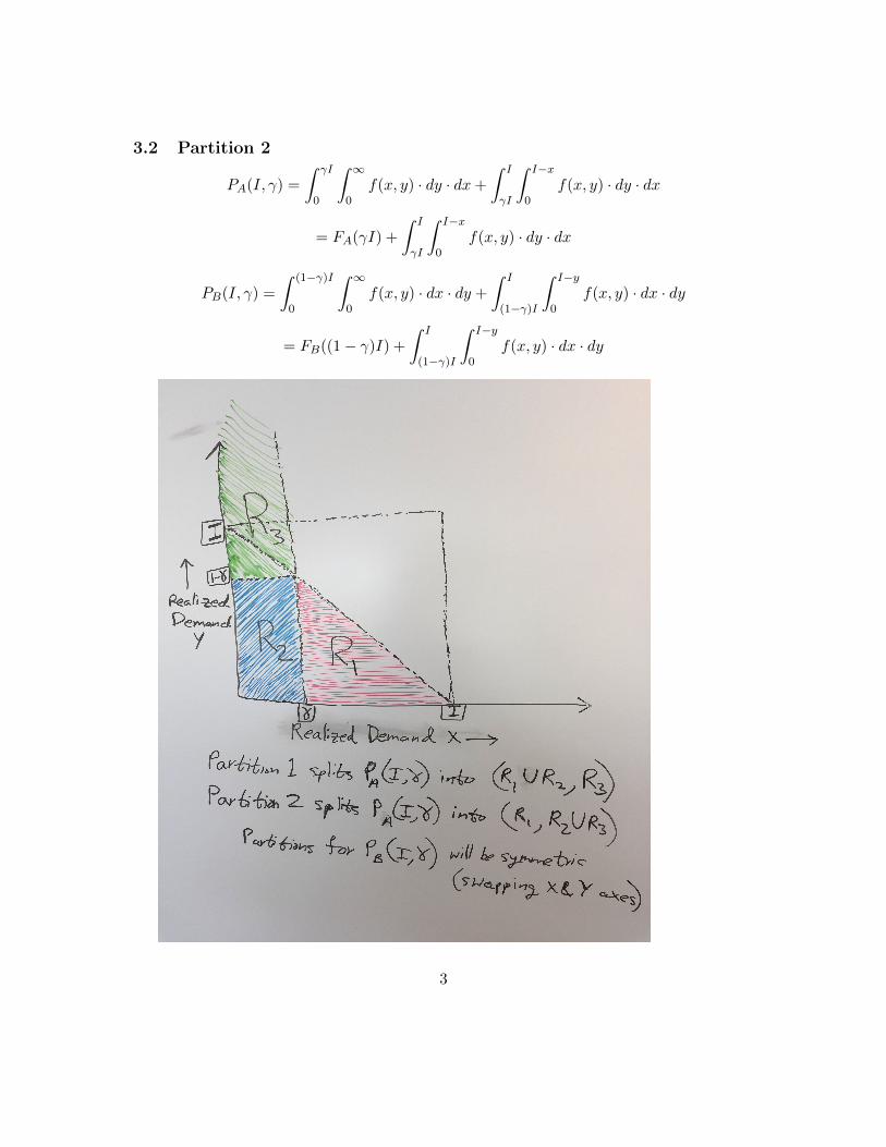
3.2 Partition 2

PA(I, γ) =

∫ γI

0

∫ ∞0

f(x, y) · dy · dx+

∫ I

γI

∫ I−x

0f(x, y) · dy · dx

= FA(γI) +

∫ I

γI

∫ I−x

0f(x, y) · dy · dx

PB(I, γ) =

∫ (1−γ)I

0

∫ ∞0

f(x, y) · dx · dy +

∫ I

(1−γ)I

∫ I−y

0f(x, y) · dx · dy

= FB((1− γ)I) +

∫ I

(1−γ)I

∫ I−y

0f(x, y) · dx · dy

3

4 Upper Bound

If we set γ = 0, we get:

PA(I, 0) = FA+B(I) ≥ αAPB(I, 0) = FB(I) ≥ αB

Therefore, when γ = 0:

I = max (F−1A+B(αA), F−1B (αB))

Similarly, when γ = 1:

I = max (F−1A (αA), F−1A+B(αB))

Therefore, allowing flexibility for 0 ≤ γ ≤ 1, we have:

I ≤ min (max (F−1A+B(αA), F−1B (αB)),max (F−1A (αA), F−1A+B(αB)))

5 Normal Distribution

If we assume that populations A and B have a normally distributed joint-demand withmeans µA, µB, standard deviations σA, σB and correlation ρ, then the upper-bound of theprevious section reduces to the minimum of the following two values:

max (µA + µB + Φ−1(αA) · σA+B, µB + Φ−1(αB) · σB)

max (µA + Φ−1(αA) · σA, µA + µB + Φ−1(αB) · σA+B)

where

σA+B =√σ2A + σ2B + 2 · σA · σB · ρ

and Φ(·) is the cumulative standard normal distribution.

6 Solution

Now we come back to the case of an arbitrary joint distribution of demand for A and B.We note that:

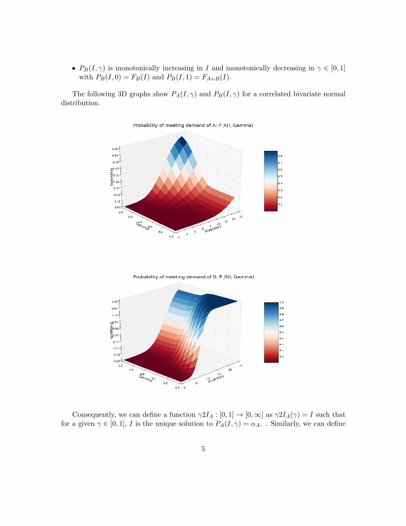
• PA(I, γ) is monotonically increasing in both I and γ ∈ [0, 1] with PA(I, 0) = FA+B(I)and PA(I, 1) = FA(I).

4

• PB(I, γ) is monotonically increasing in I and monotonically decreasing in γ ∈ [0, 1]with PB(I, 0) = FB(I) and PB(I, 1) = FA+B(I).

The following 3D graphs show PA(I, γ) and PB(I, γ) for a correlated bivariate normaldistribution.

Consequently, we can define a function γ2IA : [0, 1]→ [0,∞] as γ2IA(γ) = I such thatfor a given γ ∈ [0, 1], I is the unique solution to PA(I, γ) = αA. . Similarly, we can define

5

a function γ2IB : [0, 1] → [0,∞] as γ2IB(γ) = I such that for a given γ ∈ [0, 1], I is theunique solution to PB(I, γ) = αB. Note that:

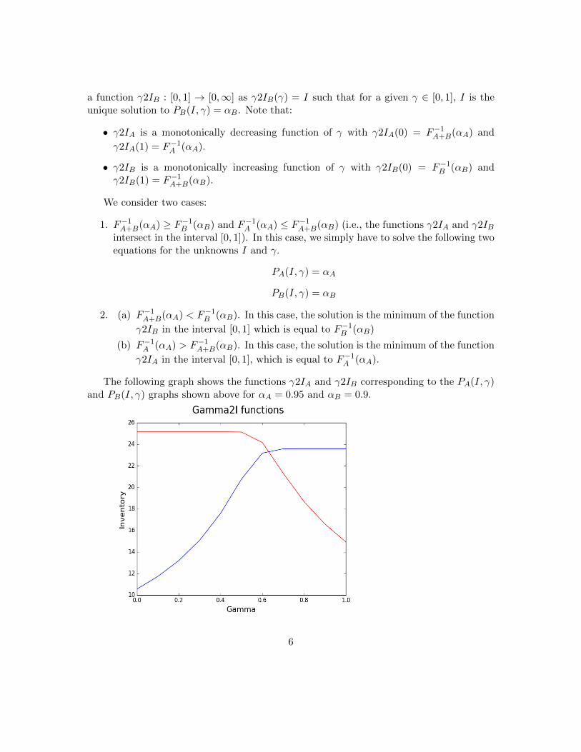
• γ2IA is a monotonically decreasing function of γ with γ2IA(0) = F−1A+B(αA) and

γ2IA(1) = F−1A (αA).

• γ2IB is a monotonically increasing function of γ with γ2IB(0) = F−1B (αB) andγ2IB(1) = F−1A+B(αB).

We consider two cases:

1. F−1A+B(αA) ≥ F−1B (αB) and F−1A (αA) ≤ F−1A+B(αB) (i.e., the functions γ2IA and γ2IBintersect in the interval [0, 1]). In this case, we simply have to solve the following twoequations for the unknowns I and γ.

PA(I, γ) = αA

PB(I, γ) = αB

2. (a) F−1A+B(αA) < F−1B (αB). In this case, the solution is the minimum of the function

γ2IB in the interval [0, 1] which is equal to F−1B (αB)

(b) F−1A (αA) > F−1A+B(αB). In this case, the solution is the minimum of the function

γ2IA in the interval [0, 1], which is equal to F−1A (αA).

The following graph shows the functions γ2IA and γ2IB corresponding to the PA(I, γ)and PB(I, γ) graphs shown above for αA = 0.95 and αB = 0.9.

6

7 More than 2 channels

Work in progress ...

7