Contents lists available at SciVerse ScienceDirect
Journal of Multivariate Analysis
journal homepage: www.elsevier.com/locate/jmva
On a dimension reduction regression with covariate adjustmentJun Zhang a, Li-Ping Zhu a,1, Li-Xing Zhu b,∗
a School of Finance and Statistics, East China Normal University, Shanghai, Chinab Department of Mathematics, Hong Kong Baptist University, Hong Kong, China
a r t i c l e i n f o
Article history:Received 10 March 2010Available online 21 June 2011
In this paper, we consider a semiparametric modeling with multi-indices when neitherthe response nor the predictors can be directly observed and there are distortions fromsome multiplicative factors. In contrast to the existing methods in which the responsedistortion deteriorates estimation efficacy even for a simple linear model, the dimensionreduction technique presented in this paper interestingly does not have to account fordistortion of the response variable. The observed response can be used directly whetherdistortion is present or not. The resulting dimension reduction estimators are shown tobe consistent and asymptotically normal. The results can be employed to test whether thecentral dimension reduction subspace has been estimated appropriately and whether thecomponents in the basis directions in the space are significant. Thus, the method providesan alternative for determining the structural dimension of the subspace and for variableselection. A simulation study is carried out to assess the performance of the proposedmethod. The analysis of a real dataset demonstrates the potential usefulness of distortionremoval.
In modern statistical data analysis, dimensionality is a vital feature in analyzing large datasets. When we aim to capturethe main relationship between the response Y and the predictor vector X in Rp with large dimension p, the smoothingmethod usually cannot be implemented in practice because of the well-known ‘‘curse of dimensionality’’. In this context,the sufficient dimension reduction method (SDR) is an effective way in reducing the dimension of the predictor vector, byreplacing the predictor vector with its projection onto a lower-dimensional subspace without loss of much information onY |X. SDR seeks a subspace S of minimal dimension satisfying YyX|PSX, where y indicates independence. Here PS standsfor the orthogonal projection onto S with respect to the usual inner product. As Cook [2] mentioned, under some mildconditions, such a subspace S uniquely exists. In the literature this subspace is called central subspace, and is denoted bySY |X. It is alsowell known that the central subspace is given by the intersection of all dimension reduction subspaces spannedby the column space of any p × k matrix B satisfying the following model
YyX|BτX. (1)
That is, conditioning on BτX, Y and X are independent, where superscript τ denotes transpose operator throughout thispaper. Moreover, B is not unique since any orthogonal transformation of B also satisfies the conditional independence (1).Thus the column space of B is concerned here rather than B itself. Denote S(B) as the space spanned by the column vectorsof B and assume that S(B) = SY |X throughout this paper.
40 J. Zhang et al. / Journal of Multivariate Analysis 104 (2012) 39–55
Li [12,14] proposed sliced inverse regression (SIR) to estimate S(B). To examine its performance, a subset of the Bostonhousing price data in [8] was analyzed for illustration. This dataset was then frequently used in the dimension reductionliterature to fit semiparametric single- or multi-index models. See [2,22] for example. In the Boston Housing Data, thereare 14 variables indicating the size, location and environment of the property as well as its selling price and other relevantvariables measuring the socioeconomic status of neighborhood (see below for more details in Section 4). The selling price isofmain interest, and thus is regarded as the response Y . As Li [12,14] pointed out, by directlymodeling this datasetwith other13 predictors, a nonparametric regression cannot be efficiently estimated. On the other hand, he found a linear combinationof the predictors fromwhich the information on the selling price may be captured. See also [2]. We will re-analyze this datain Section 4 with a different perspective and explanation.
There are a number of estimation proposals for S(B) available in the literature, such as sliced inverse regression (SIR, [12]),sliced average variance estimation (SAVE, [3]), minimum average variance estimation (MAVE, [24]), contour regression [9],directional regression [10], discretization–expectation estimation (DEE, [30]), and cumulative slicing estimation (CSE, [29]).These methods preserve the root-n consistency and the computational cost is not high. Once the central subspace has beenidentified, subsequent analysis with the low-dimensional coordinates BτX can be performed.
However, in many applications, response and predictors may not be directly observed, but only with certaincontamination. One scenario is that there are some additive measurement errors in both response and predictors. In sucha setting Li and Carroll [1] first investigated an estimation of S(B) using SIR, Lue [15] suggested using principal Hessiandirections (pHd, [12,13]) to handle this problem. Li and Yin [11] provided a general invariant law between surrogate andordinary dimension reduction subspace. In the scenario considered in this paper, both response and predictors are distortedby certain multiplicative distorting functions. Formally:Y = φ(U)Y ,
X = ψ(U)X,Uy(X, Y ),
(2)
where Y is the unobserved continuous response, X = (X1, X2, . . . , Xp)τ is the unobserved continuous predictor vector in
Rp, U is an observed continuous scalar confounding variable, and (Y , X) are the actual observed response and predictors.ψ(U) is a p × p diagonal matrix diag
ψ1(U), . . . , ψp(U)
, where φ(·) andψr(·) denote the unknown continuous distorting
functions. The diagonal form ofψ(U) indicates that the confounding variable U distorts each component of the unobservedpredictors X in a multiplicative fashion, see [16–18]. More general settings with correlated ψ(·)’s and/or with differentconfounding variables for different predictors and response are worthwhile to investigate. These will be the topics of futureresearch. Based on the estimation method by Cui et al. [4], it is possible to derive consistent estimation of the multi-indices.However, somemore technical skills for theoretical development are necessary. Thus, the relevant investigation will not becovered in this paper.
The above scenario is not uncommon in practice due to the distortion from the effects of confounding variable. Forinstance, the analysis of the Boston Housing data in [17] shows this phenomenon. In this paper we will also analyze theBoston Housing data by utilizing a model that includes a confounding variable into a semiparametric model structure. Theanalysis, along with some comparisons and discussion, is presented in Section 4. It is clear that a suitable adjustment for theobserved (distorted) Y response and the (distorted) predictor vector X is necessary to reduce the non-negligible estimationbias. Sentürk andMüller [18] proposed a covariate adjustment for the linear model via a connection to a varying-coefficientregression. Further, by using a binning method that is similar to that proposed in [5] for longitudinal data, Sentürk andMüller [17] investigated correlation analysis for this linear covariate-adjusted model, as indicated above. Li [12,14], incontrast, found a nonlinear structure in this dataset without taking the predictor distortion into account. For robustnessconsiderations, he then fitted a very general semiparametric model by using SIR. However, we will see in Section 4 thatwhen distorting functions are introduced into the model, the estimation and data analysis are very different from thosein [12,14].
As is described above, of primary interest here is the creation of a dimension reduction technique to explore therelationship between the response and the predictors of interest. Note that there is no specific model assumption betweenY and X in model (1) such as linear or generalized linear structure. The binning technique to covariate-adjusted varying-coefficient model or generalized covariate-adjusted model used in [16–19] cannot be implemented here to deal withdimension reduction and estimating the subspace S(B). In contrast, the direct estimation procedure proposed by Cui et al. [4]works for this problem. The key idea of the direct estimation procedure is to obtain consistent estimators of the unobserved(Y ,X), which are denoted by Y = Y/φ(U) and X = ψ(U)−1X, where φ(·) and ψ(·) are the kernel smoothing estimators.Any further estimation is then based on the estimated response and predictors. As our model is very general with nonlinearstructure, we should consider adopting this direct estimation method to deal with the distortion. To this end, we estimateS(B) by regressing the observed Y and X against the confounding variable U by utilizing a method of least squares type.An interesting finding is that even the response has distortion, our estimation based on the dimension reduction approachcan simply use the distorted response without a deterioration of estimation effect. This is very different from all existingmethods even for the linear model. The new method is easy to implement as the least squares method is. The asymptoticnormality of the relevant estimators is also obtained. Furthermore, a re-visit to the Boston Housing data shows that after
J. Zhang et al. / Journal of Multivariate Analysis 104 (2012) 39–55 41
removing the distortion, the index of interest in the model has a different and more reasonable explanation as comparedto [14].
The remainder of the paper is organized as follows. In Section 2, we explain the rationale behind the proposed estimationmethod, and illustrate its theoretical foundations at the population level. Next, we present the estimation procedure atthe sample level. The asymptotic properties are also investigated in this section. In Section 3, we then provide simulationstudy for illustration. Detailed analysis of the Boston Housing data is reported in Section 4. All of the technical proofs of theasymptotic results are given in the Appendix.
2. Methodology development
2.1. Method at the population level
We recommend the following methods to identify the dimension reduction subspace of model (1).
2.1.1. The case without distortionConsider the first derivative of the conditional distribution of Y given X. Note that if the conditional distribution
FY |X(y|x) = FY |BτX(y|Bτ x) of Y , given X = x, is continuous with respect to x, its derivative is equal to ∂FY |X(y|x)/∂x =
B∂FY |BτX(y|Bτ x)/∂(Bτ x). In otherwords, its derivative lies in the space S(B).We start ourmotivation fromnormal distributionof X with mean EX and identity covariance matrix Ip. The normality assumption will later be replaced by more generaldistribution assumption. Stein’s Lemma 4 [21] shows that
E∂F(y|X)/∂X
= E
(X − EX)F(y|X)
= E
(X − EX)I(Y ≤ y)
.
Based on [28,23], we know that the normality assumption can be relaxed to the popular linearity condition (see [12]):
E(X − EX)|BτX
= PτB (ΣX)(X − EX), (3)
where PB(ΣX) = B(BτΣXB)−1BτΣX and ΣX = Cov(X), and ΣX here is a positive definite matrix. The linearity condition(3) is mild, particularly for high-dimensional predictors. That is, this condition holds when X is elliptically distributed. Formore general distribution of X, Hall and Li [7] proved that this condition holds approximately when the dimension p of X islarge.
Conditions (3) and (1) entail the following equation:
3(y) := E(X − EX)1{Y ≤ y}
= E
1{Y ≤ y}E
(X − EX)|(BτX, Y )
= E
1{Y ≤ y}E
(X − EX)|BτX
= PτB (ΣX)E
(X − EX)1{Y ≤ y}
.
We then identify S(B) by
Σ−1X 3(y) = Σ−1
X E(X − EX)1{Y ≤ y}
= B(BτΣXB)−1BτE
(X − EX)1{Y ≤ y}
⊆ S(B). (4)
Hence,Σ−1X 3(y) can be used to identify base directions of S(B) at population level, see e.g. [23]. From this explanation, we
can see that the eigenvectors that are associated with the first largest k eigenvalues of
Σ−1X E
3(Y o)3(Y o)τ
Σ−1
X
can be base directions of S(B), where Y o is an independent copy of Y . We state the relevant results in the following theorem.
Theorem 1. Assume that the predictor vector X satisfies the linearity condition (3), andΣX is a positive definite matrix. We thenhave, for all y, span
Σ−1
X 3(y)
⊆ S(B). Recall that Y o is defined as an independent copy of Y , and let 3 := E3(Y o)3τ (Y o)
.
The kernel matrixΣ−1X 3 satisfies that span(Σ−1
X 3) ⊆ S(B).
Theorem 1 indicates that when the first k eigenvalues ofΣ−1X 3 are nonzero, the associated eigenvectors can be used to
identify S(B).
2.1.2. The case with distortionWhen the response and predictors are distorted by a confounding variable,we first examine kernelmatrix to see howbias
occurs when distorted variables are used. As Sentürk and Müller [16,18] suggested, we also assume that, for the predictorvector X, the distorting function satisfies
Eψ(U) = Ip.
42 J. Zhang et al. / Journal of Multivariate Analysis 104 (2012) 39–55
The identifiability condition ensures that the distorting effect vanishes with no average distortion, namely, EX = EX.Appealing to the independence between U and (X, Y ), we have
3(y) := E(X − EX)1{Y ≤ y}
= E
1{Y ≤ y}E
(X − EX)|(Y ,U)
= E
1{Y ≤ y}ψ(U)E
(X − EX)|(Y ,U)
+ E
1{Y ≤ y}
ψ(U)− Ip
EX
= E
ψ(U)PτB (ΣX)1{Y ≤ y}(X − EX)
+ E
1{Y ≤ y}(ψ(U)− Ip)
EX. (5)
From the equations in (5), we can see that bias exists when (Y , X) is used since ψ(U) is not identical to Ip in this distortingcase. In other words,Σ−1
X 3(y) ⊆ S(B), and it cannot identify base directions of S(B).To find the subspace S(B), we can naturally use both the estimators of X and Y by the kernel smoother proposed by Cui
et al. [4] for the parametric model. Interestingly, our method does not require to explicitly account for the distortion of theresponse variables. Under the linearity condition (3) on X, it is easy to see that
�(y) := E(X − EX)1{Y ≤ y}
= E
1{Y ≤ y}E
(X − EX)|(Y ,U)
= E
1{Y ≤ y}E
(X − EX)|Y
= PτB (ΣX)E
1{Y ≤ y}(X − EX)
,
i.e., Σ−1X �(y) ⊆ S(B). This property simplifies the estimation procedure, since we only need to estimate the unobserved
predictor vector X and can directly use the observed response Y . It is worth mentioning that none of the existing methodsshares this feature, not even the ones designed for a parametric model. The following theorem summarizes this discussion.
Theorem 2. Assume that the predictor vector X satisfies the linearity condition (3), and ΣX is a positive definite matrix. Then,for the model satisfying (1) and (2), we have span
Σ−1
X �(y)
⊆ S(B). Equivalently, let Y o be an independent copy of Y , and� := E
�(Y o)�τ (Y o)
. Then the kernel matrixΣ−1
X � satisfies span(Σ−1X �) ⊆ S(B).
Remark 1. Theorem 2 permits us to apply a spectral decomposition on the kernel matrix Σ−1X � to seek the space S(B).
That is, letting b1, . . . , bk be the eigenvectors ofΣ−1X � that corresponds to the first largest k nonzero eigenvalues, the space
S(b1, . . . , bk) spanned by b1, . . . , bk may recover S(B).
2.2. Estimation procedures and asymptotic properties
Different from Section 2.1, we present the estimation procedure and results in the case with distortion first and regardthe case without distortion as its special case.
2.2.1. The case with distortionSuppose that we have the following independent observations: for i = 1, . . . , n,Yi = φ(Ui)Yi,
Xi = ψ(Ui)Xi,Uiy(Xi, Yi).
As was discussed in Section 2.1.2, we need to estimate the unobserved predictor vector X. Note that X = (X1, X2, . . . , Xp)τ ,
ψr(U) and Xr for r = 1, . . . , p can easily be rewritten as
ψr(U) = E[Xr |U]/EXr = E[Xr |U]/EXr ,
Xr = Xr/ψr(U), r = 1, . . . , p.
Thus, estimating X involves estimating ψr(·) and EXr . We follow the estimation procedure in [4] to estimate the distortingfunctions ψr(u)’s. For convenience, we denote the density function of U by η(u) and
gr(u) = E(Xr |U = u)η(u), 1 ≤ r ≤ p. (6)Let
gr(u) =1nh
n−i=1
Ku − Ui
h
Xri, η(u) =
1nh
n−i=1
Ku − Ui
h
, (7)
E[Xr ] =¯X r =
1n
n−i=1
Xri, E(Xr |U = u) =gr(u)η(u)
, (8)
J. Zhang et al. / Journal of Multivariate Analysis 104 (2012) 39–55 43
and define
ψr(u) =
E(Xr |U = u)E[Xr ]=
gr(u)η(u)
×1¯X r
, r = 1, . . . , p, (9)
where h is the bandwidth and K(·) is the kernel function. Note that η(u) is the kernel estimator of η(u), and gr(u) is theestimator of gr(u), for r = 1, . . . , p. Based on the estimator ψr(u) for r = 1, . . . , p, we obtain the estimators of Xi and theestimator of ψ(·) by, for i = 1, . . . , n,
Xi = ψ−1(Ui)Xi,
ψ(Ui) = diag(ψ1(Ui), . . . , ψp(Ui)). (10)
Consequently, the estimators ofΣX, �(y) and � in Theorem 2 are defined as
ΣXn =1n
n−i=1
[Xi − X][Xi − X]τ , X = (
¯X1, . . . ,¯Xp)
τ ,
�n(y) =1n
n−i=1
[Xi − X]I(Yi ≤ y), �n =1n
n−s=1
�n(Ys)�
τn(Ys)
. (11)
Theorem 3. In addition to the conditions of Theorem 2, assume conditions (A1)–(A4) in the Appendix. Then we have
Σ−1Xn
�nP
−→Σ−1X �.
This theorem states the convergence of the estimated kernel matrix Σ−1Xn
�n. We use the k eigenvectors (b1, . . . , bk) of
Σ−1Xn
�n corresponding to its k nonzero eigenvalues λ1, . . . , λk as the estimators of basis directions in S(B). Note that thesequantities are connected through the equations
�nbi = λiΣXnbi, i = 1, . . . , k.
The next theorem presents the asymptotic normality of the eigenvectors bi. For its formulation we need the followingdefinition. Let (Y o
1 ,Xo1), (Y
o2 ,X
o2) be independent copies of (Y ,X). We define
u1(Xo
1 − EXo1, Y
o1 )
=
13
(Xo
1 − EXo1)E
I{Y o
1 ≤ Y o2 }�τ (Y o
2 )|(Xo1 − EXo
1, Yo1 )
+ E
�(Y o
2 )I{Yo1 ≤ Y o
2 }|(Xo1 − EXo
1, Yo1 )
(Xo
1 − EXo1)τ+ �(Y o
1 )�τ (Y o
1 )− 3�
× bi (12)
and its covariance matrix
Qi := Covu1(Xo
1 − EXo1, Y
o1 )
= Eu1
(Xo
1 − EXo1, Y
o1 )
uτ1
(Xo
1 − EXo1, Y
o1 )
(13)
Eu1(Xo
1 − EXo1, Y
o1 )
= 0 are used in the last step above.
Theorem 4. Assume that the conditions of Theorem 3 hold. Let e denote a unit vector orthogonal to S(B). Then√neτ bi
d−→N(0, Si) (14)
where Si =1λ2ieτΣ−1
X QiΣ−1X e, i = 1, . . . , k with λi and Qi denoting the ith largest distinct nonzero eigenvalues of Σ−1
X � and the
covariance matrix defined in (13) above.
Remark 2. It is worthmentioning that this result can also be used for determining the structural dimension of the subspaceS(B) and for testing the significance of the components of b1, . . . , bk for variable selection. The idea is as follows. Suppose
that an estimator of Si in (14) is obtained, denoted by Si. Let vector e be orthogonal to S(B). The value of√neτ bi/
Si can
be used to decide which bi identifies S(B) appropriately and then to determine the structural dimension of the subspaceS(B). Moreover, for variable selection, we can take e to be the vector vj of 0’s except for the jth position with value 1 to testwhether the jth component of bi is zero or not. We use this result in our real data analysis in the next section.
Estimation of Si. An estimator for Si can be constructed as follows. From (12) we can see that we need to estimate theconditional expectation E
�(Y o
2 )I{Yo1 ≤ Y o
2 }|(Xo1 − EXo
1, Yo1 )
. Recall that (Y o
1 ,Xo1) is independent of (Y o
2 ,Xo2). Thus we
44 J. Zhang et al. / Journal of Multivariate Analysis 104 (2012) 39–55
have
5�(y) = E�(Y o
2 )I{Yo1 ≤ Y o
2 }|(Xo1 − EXo
1, Yo1 = y)
= E
�(Y o
2 )I{y ≤ Y o2 }|(Xo
1 − EXo1, Y
o1 = y)
= E
�(Y o
2 )I{y ≤ Y o
2 }.
An estimator of 5�(y) is given by
5�(y) =1n
n−s=1
�n(Ys)I{y ≤ Ys}. (15)
Thus, from (12), an estimator of u1(Xo
1 − EXo1, Y
o1 )
can be defined as
u1(X1 − X, Y1)
=
13
(X1 − X)5�
τ(Y1)+ 5�(Y1)(X1 − X)τ + �n(Y1)�
τn(Y1)− 3�n
× bi. (16)
Then from (13), Qi and Si can be estimated by
Qi =1n
n−t=1
u1(Xt − X, Yt)
uτ1
(Xt − X, Yt)
,
Si =1
λ2i
eτΣ−1Xn
QiΣ−1Xn
e.
The following theorem states the estimation consistency.
Theorem 5. Under the conditions of Theorem 4, and assuming that E(XτX)2 < ∞, we have
SiP
−→ Si, for i = 1, . . . , k.
2.2.2. The case without distortionWhen the distorting functions are equal to 1, the problem is reduced to the classical case with the observed (X, Y ), and
3(y) = 3(y). Thus, the bias in the formula of (5) vanishes, and from (4),Σ−1X 3(y) can be used to find base directions of S(B).
Although this is a special case at the population level, the asymptotic behavior cannot simply be derived directly from theobtained results because it is greatly affected by the involved nonparametric estimation, andwe require different argumentsfor the technical proof. To make the relevant results available, we state them as propositions parallel to Theorems 3–5.
When the independent sample {(Xi, Yi)}ni=1 is available, according to Theorem 1, the relevant estimators are as
ΣXn =1n
n−i=1
[Xi − X][Xi − X]τ , X = (X1, . . . , Xp)
τ ,
3n(y) =1n
n−i=1
[Xi − X]I(Yi ≤ y), 3n =1n
n−s=1
3n(Ys)3
τn(Ys)
. (17)
Proposition 1. Under the conditions of Theorem 1, and E(XXτ ) < ∞, we have
Σ−1Xn 3n
P−→Σ−1
X 3.
This proposition states the convergence of the estimated kernel matrix Σ−1Xn 3n under the assumption of without
distortion. We use the k eigenvectors (b∗
1, . . . , b∗
k) of Σ−1Xn 3n corresponding to its k nonzero eigenvalues λ∗
1, . . . , λ∗
k as theestimators of basis directions in S(B), which are connected through the equations
3nb∗
i = λ∗
i ΣXnb∗
i , i = 1, . . . , k.
Consider the asymptotic normality of the eigenvectors b∗
i . In parallel, let (Y o1 ,X
o1), (Y
o2 ,X
o2) be independent copies of (Y ,X).
Define
u∗
1
(Xo
1 − EXo1, Y
o1 )
=
13
(Xo
1 − EXo1)E
I{Y o
1 ≤ Y o2 }3τ (Y o
2 )|(Xo1 − EXo
1, Yo1 )
+ E
3(Y o
2 )I{Yo1 ≤ Y o
2 }|(Xo1 − EXo
1, Yo1 )
(Xo
1 − EXo1)τ+ 3(Y o
1 )3τ (Y o
1 )− 33
× b∗
i (18)
J. Zhang et al. / Journal of Multivariate Analysis 104 (2012) 39–55 45
and its covariance matrix
Wi = Covu∗
1(Xo1 − EXo
1, Yo1 )
= Eu∗
1
(Xo
1 − EXo1, Y
o1 )
u∗τ1
(Xo
1 − EXo1, Y
o1 )
, (19)
with Eu∗
1
(Xo
1 − EXo1, Y
o1 )
= 0. Analogous to Theorem 4, we have the following results.
Proposition 2. Assume that the conditions of Proposition 1 hold. Let e denote a unit vector orthogonal to S(B). Then√neτ b∗
id
−→N(0, Ti) (20)
where Ti =1λ∗2ieτΣ−1
X WiΣ−1X e, i = 1, . . . , k with λ∗
i and Wi denoting the ith largest distinct nonzero eigenvalues of Σ−1X 3 and
the covariance matrix defined in (19).
Estimation of Ti. From (18), we need to construct an estimator of u∗
1
(Xo
1 − EXo1, Y
o1 )
. Similar to (15) and (16), we estimate
u∗
1
(Xo
1 − EXo1, Y
o1 )
by
u∗
1
(X1 − X, Y1)
=
13
(X1 − X)53
τ(Y1)+ 53(Y1)(X1 − X)τ + 3n(Y1)3
τn(Y1)− 33n
× b∗
i
with 53(y) =1n
∑ns=1 3n(Ys)I{y ≤ Ys}. Then, the estimators ofWi and Ti are defined as
Wi =1n
n−t=1
u∗
1
(Xt − X, Yt)
u∗τ1
(Xt − X, Yt)
,
Ti =1
λ∗2i
eτΣ−1Xn WiΣ
−1Xn e.
The following result is about the estimation consistency.
Proposition 3. Under the conditions of Proposition 1, and assuming that E(XτX)2 < ∞, we have
TiP
−→ Ti, for i = 1, . . . , k.
3. Simulation study
Example. Here we present a simulation study to assess the performance of the proposed method for estimating the centralspace. To measure estimation accuracy, the trace correlation criterion is applied (see [6]), that is, R2(k) = trace(PBPB)/k,where B is a p×kmatrix spanning S(B),B is a p×kmatrixwhose columns are the eigenvectors associatedwith the k nonzeroeigenvalues of Σ−1
Xn�n, and, as previously defined, matrix PB is the projection operator in the standard inner product of B.
Thus, the closer the R2(k) value is to 1, the better the performance of k nonzero eigenvalues ofΣ−1Xn
�n is. We also examinethe performance when the dimension p of predictors X = (X1, . . . , Xp)
τ grows with p = 10, 20, 30. In these simulations,we make no comparisons with other possible competitors, because there is no other method available for such a problemwith distortion. On the other hand, it is clear that when model structure is assumed to be given, we should use parametricmodel to have better estimation performance.
Consider the following five models.
Y =12X1 +
12X2 +
12X3 +
12X4 + ε (21)
Y = exp2√13
X1−3√13
X2+ε (22)
Y = sin
1√2X1 −
1√2X2 +
13
× ε
(23)
Y = log(|X1 − 4|)+ 0.5 × ε (24)
Y = (X1 − 5)/
1√2X2 −
1√2X3 + 1
+ 0.5 × ε. (25)
In this example, we generate the predictors Xij from t-distribution 6 + t(5) with mean 6 and truncated in the interval[0.8360, 11.1641], i = 1, . . . n, j = 1 . . . p, and the model error ε is from normal distribution N(0, 1.44). The confoundingvariable U is drawn from a Uniform(1, 6), the distortion function for the response Y is φ(U) =
(U+1)2
22.3333 , and those for the
46 J. Zhang et al. / Journal of Multivariate Analysis 104 (2012) 39–55
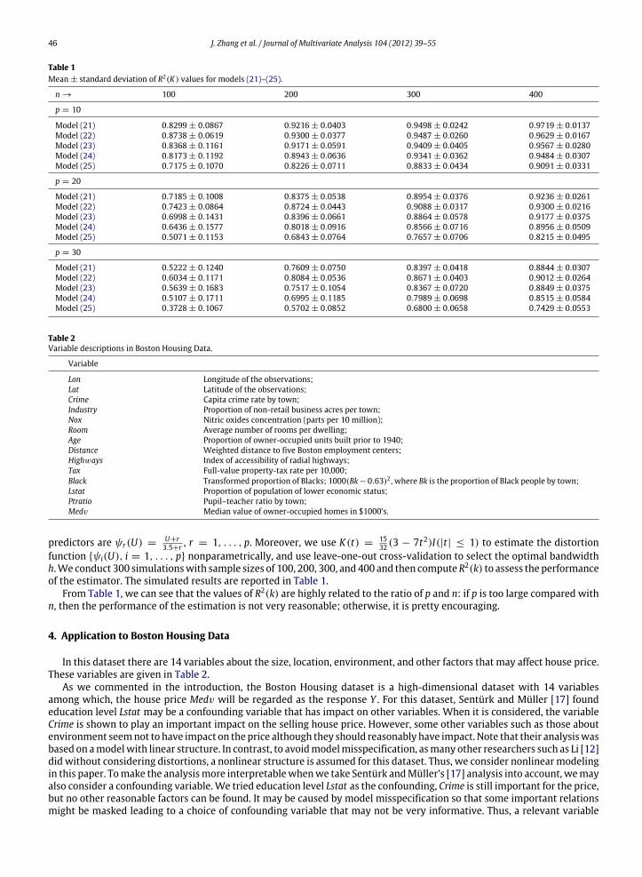
Table 1Mean ± standard deviation of R2(K) values for models (21)–(25).
Table 2Variable descriptions in Boston Housing Data.
Variable
Lon Longitude of the observations;Lat Latitude of the observations;Crime Capita crime rate by town;Industry Proportion of non-retail business acres per town;Nox Nitric oxides concentration (parts per 10 million);Room Average number of rooms per dwelling;Age Proportion of owner-occupied units built prior to 1940;Distance Weighted distance to five Boston employment centers;Highways Index of accessibility of radial highways;Tax Full-value property-tax rate per 10,000;Black Transformed proportion of Blacks; 1000(Bk−0.63)2 , where Bk is the proportion of Black people by town;Lstat Proportion of population of lower economic status;Ptratio Pupil–teacher ratio by town;Medv Median value of owner-occupied homes in $1000’s.
predictors are ψr(U) =U+r3.5+r , r = 1, . . . , p. Moreover, we use K(t) =
1532 (3 − 7t2)I(|t| ≤ 1) to estimate the distortion
function {ψi(U), i = 1, . . . , p} nonparametrically, and use leave-one-out cross-validation to select the optimal bandwidthh.We conduct 300 simulationswith sample sizes of 100, 200, 300, and 400 and then computeR2(k) to assess the performanceof the estimator. The simulated results are reported in Table 1.
From Table 1, we can see that the values of R2(k) are highly related to the ratio of p and n: if p is too large compared withn, then the performance of the estimation is not very reasonable; otherwise, it is pretty encouraging.
4. Application to Boston Housing Data
In this dataset there are 14 variables about the size, location, environment, and other factors that may affect house price.These variables are given in Table 2.
As we commented in the introduction, the Boston Housing dataset is a high-dimensional dataset with 14 variablesamong which, the house price Medv will be regarded as the response Y . For this dataset, Sentürk and Müller [17] foundeducation level Lstat may be a confounding variable that has impact on other variables. When it is considered, the variableCrime is shown to play an important impact on the selling house price. However, some other variables such as those aboutenvironment seemnot to have impact on the price although they should reasonably have impact. Note that their analysiswasbased on amodelwith linear structure. In contrast, to avoidmodelmisspecification, asmany other researchers such as Li [12]did without considering distortions, a nonlinear structure is assumed for this dataset. Thus, we consider nonlinearmodelingin this paper. Tomake the analysismore interpretablewhenwe take Sentürk andMüller’s [17] analysis into account, wemayalso consider a confounding variable.We tried education level Lstat as the confounding, Crime is still important for the price,but no other reasonable factors can be found. It may be caused by model misspecification so that some important relationsmight be masked leading to a choice of confounding variable that may not be very informative. Thus, a relevant variable
J. Zhang et al. / Journal of Multivariate Analysis 104 (2012) 39–55 47
about education efficiency and quality Ptratio ‘‘pupil–teacher ratio by town’’ is considered. This variablemay influence otherfactors. Let Ptratio ‘‘pupil–teacher ratio by town’’ as U and the other 12 variables are the predictors X. As the confoundingvariablewe use is different from that used by Sentürk andMüller [17], we alsomake a comparison of the resulting estimatorsof S(B) to see why our choice of the confounding variable Ptratio is more reasonable.
To determine whether or not the confounding variable has impact on the dimension k of S(B) in model (1), we considertwo cases: with and without confounding variable U . In both the settings, we employ two methods to estimate k, that is,the bootstrap method proposed by Ye and Weiss [25] and the BIC-type criterion proposed by Zhu et al. [26], see the detailsin these two references. For the bootstrap method, we generate 200 bootstrapping samples. Both the methods result in theconclusion that the dimension k of S(B) is one whether the confounding variable is included, thus k = 1 is used.
As Ptratio is suggested as our confounding variable, we use the notations BPt,1 and BPt,0 for the estimated base directionsof S(B) with or without distortion of Ptratio, respectively. Note that Sentürk and Müller [17] used Lstat: ‘‘proportion ofpopulation of lower educational status’’ as a confounding variable for correlation and partial correlation analyses. As theymainly investigated the relation between housing price and crime rate in a linear structure, such a choice is reasonable.However, as this dataset has been intensively studied and nonlinear structure has been explored in the literature, to avoidmodel misspecification issue, we still consider semiparametric modeling. To see which one is more reasonable, we make acomparison with Lstat by presenting the estimated base directions of S(B) when Lstat is used as the confounding variable.Similar to BPt,1 and BPt,0, denote BLs,1 and BLs,0 as the estimator of S(B)with andwithout distortion of Lstat . The estimator BPt,0
and BLs,0 are obtained by the estimation procedure in Section 2.2.2, and BPt,1 and BLs,1 are obtained by the semiparametricestimation procedure in Section 2.2.1. We present the linear combinations: BτPt,0X, B
τPt,1X, B
τLs,0X and BτLs,1X, respectively as
follows. Standard errors are in parentheses:
BτPt,0X = − 0.9302Lon(0.1369)
+ 0.2374Lat(0.1631)
− 0.0026Crim(0.0030)
− 0.0043Industry(0.0030)
− 0.2539Nox(0.2477)
+ 0.1032Room(0.0213)
− 0.0024Age(0.0006)
− 0.0456Distance(0.0093)
+ 0.0115Highways(0.0042)
− 0.0008Tax(0.0002)
+ 0.0005Black(0.0002)
− 0.0327Lstat(0.0039)
BτPt,1X = − 0.3168Lon(0.1829)
− 0.0143Lat(0.2061)
− 0.0132Crim(0.0064)
− 0.0082Industry(0.0032)
− 0.9432Nox(0.3301)
+ 0.0589Room(0.0250)
− 0.0021Age(0.0006)
− 0.0700Distance(0.0127)
+ 0.0173Highways(0.0051)
− 0.0011Tax(0.0002)
+ 0.0004Black(0.0002)
− 0.0302Lstat(0.0040)
BτLs,0X = − 0.3386Lon(0.1278)
+ 0.0651Lat(0.1464)
− 0.0055Crim(0.0026)
− 0.0021Industry(0.0027)
− 0.9143Nox(0.2324)
+ 0.1987Room(0.0182)
− 0.0044Age(0.0006)
− 0.0575Distance(0.0085)
+ 0.0143Highways(0.0039)
− 0.0007Tax(0.0002)
− 0.0462Ptratio(0.0063)
+ 0.0007Black(0.0002)
BτLs,1X = − 0.5582Lon(0.1726)
+ 0.4307Lat(0.1882)
− 0.0029Crim(0.0033)
− 0.0003Industry(0.0021)
− 0.7019Nox(0.2770)
+ 0.0817Room(0.0285)
− 0.0003Age(0.0005)
− 0.0397Distance(0.0130)
+ 0.0184Highways(0.0043)
− 0.0007Tax(0.0002)
− 0.0403Ptratio(0.0086)
+ 0.0003Black(0.0002)
To see the relationship between the house price and other factors, we consider the loadings on the variables to see
their significance by testing. From Theorems 4 and 5, we can construct test statistic√neT BPt,1/
S1 for every individual
component of BPt,1 in this direction by choosing vector e = (0, . . . , 0, 1, 0, . . . , 0)T , where 1 is the jth element of the vectore for j = 1, . . . , p. When the significance level is set at 0.05, we find that the location indices Lon and Lat are insignificant,whereas the social environmentCrime, the natural environment index Industry and the air pollution indexNox are significant.In contrast, if we consider Lstat as the confounding variable, Crime and Industry are insignificant whereas Lon, Lat and Noxare significant. Note that the natural index Industry, the social environment Crime and the air pollution index Nox are allreasonably highly related to life quality and then house price. The significance of these indices Crime, Industry and Nox inBPt,1 are very reasonable.
We note that the result of this analysis differs from the correlation and partial correlation analysis in [17]. In theiranalysis Lstat was used as the confounding variable, and it was found that Crime and the house priceMedv has a significantnegative relationship. However, their analysis was based on a linear model structure so that the correlation and partialcorrelation analysis can be performed. Their analyses did not consider the impact from other factors such as the naturalindex Industry and the air pollution index Nox together. Our analysis indicates that there is a nonlinear pattern between theestimated response Y and the linear combination BτPt,1X. To be precise, using the estimation procedure of (10), we obtain theestimated X and Y , which are denoted as X and Y , and use the kernel estimation to estimate E(Y |BτX)with ‘‘synthetic’’ data
48 J. Zhang et al. / Journal of Multivariate Analysis 104 (2012) 39–55
Fig. 1. The kernel smoothing curve (solid line) of the estimated response Medv: Y against estimated linear combination: BτPt,1X, along with 95% pointwiseconfidence interval (dotted lines), and a linear fitting Y against BτPt,1X (straight line).
{Yi, BτPt,1Xi}ni=1. The curve pattern of Y against BτPt,1X is presented in Fig. 1, in which we depict the kernel smoothing curve
(solid line) and its 95% confidence bands (dotted lines). We also fit a linear regression and display the straight line. From thisfigure, we see that the straight line is not encapsulated within the bands, suggesting that the linear regression may not beadequate for fitting this dataset. Altogether, we may consider the education level factor Ptratio as a reasonable confoundingvariable.
To make a comparison with the case without distortion, we analyze the dataset by ignoring the effect of confoundingvariable by assuming φ(·) ≡ 1 and ψi(·) ≡ 1 for i = 1, . . . , p, using similar tests for the loadings, with the standarderror of BPt,0 that can be obtained from the asymptotic normality of Proposition 2, we can then see that Lat , Crime, Industryand Nox are insignificant at the 0.05 level, whereas the location index Lon in BPt,0 and BLs,0 is fairly significant. Thus suchloadings on the linear combination seems not reasonable. Li [14, Chapter 4] applied the SIR method to this dataset withoutconsidering distorting influence of the confounding variable. Similar conclusion to that based on BτPt,0X can be made, andthe air pollution index Nox is insignificant although Nox should be an important factor affecting house price. Therefore, theconfounding variable does have impact so that the significant predictors can really be revealed in themodel and any furtheranalysis can be more meaningful.
5. Discussions
In this paper, we propose a dimension reduction approach to construct an estimation of unknown parameters ofinterest in a very general multi-index model when both response and predictors are distorted and then cannot be directlyobserved. An interesting result is that when ourmethod is used, we can simply use distorted response in estimationwithoutdeterioration of estimation effect whereas all existingmethods have to take care of that distortion evenwhen a linearmodelis used. This somewhat surprising feature of our method is worthy of further investigations.
To remove distortion, we adopt a direct estimation procedure suggested by Cui et al. [4]. The advantage of this methodis that it can handle such semiparametric models whereas the method by Sentürk and Müller [16,17] may not be able todeal with these models. However, it involves nonparametric smoothing and then when the dimension of U is also large,estimation efficiency is a concern. This is a typical issue for nonparametric estimation and in general there is no other bettersolution. However, it is of interest to explore solutions for models with particular structures.
Another issues concerns the choice of confounding variable. In the literature, one common confounding variable is used.However, in practice, different variables or responses may have different confounding variables. In principle, our approachcan handle this case because the method by Cui et al. [4] can be applied to deal with this. However, deriving asymptoticnormality of the corresponding estimators involves additional technicalities that go beyond the scope of the current paper.Therefore this case will be considered in future research.
Acknowledgments
The first two authorswere supported by theNational Social Science Foundation of China (08CTJ001). The third authorwassupported by an RGC grant from the Research Grants Council of Hong Kong, Hong Kong, China. The authors thank the editorand two referees for their constructive comments and suggestions which led to an improved version of an early manuscript.A special thank goes to the editor who provided the generous help on editing the manuscript.
J. Zhang et al. / Journal of Multivariate Analysis 104 (2012) 39–55 49
Appendix
In this section we provide the rigorous proofs for our main results. First we present the additional regularity conditionsneeded. For simplicity, throughout these proofs, let X0
= X − EX and X0i = Xi − EX, for i = 1, . . . , n. The following are the
regularity conditions other than those stated in the theorems and propositions.(A1) For r = 1, . . . , p, the distorting functionψr(u), the density function η(u) of U and gr(u) defined in (6) are greater than
a positive constant and 3-times differentiable. Moreover, their third derivatives satisfy the following Lipschitz-typecondition: there exists a neighborhood of the origin, sayΘ , and a constant c > 0 such that for any ϵ ∈ Θ
|η(3)(u + ϵ)− η(3)(u)| < c|ϵ|,|g(3)r (u + ϵ)− g(3)r (u)| < c|ϵ|, r = 1, . . . , p.
(A2) The continuous kernel function K(·) satisfies: K(·) is symmetric about zero, and its support is the interval [−1, 1].Furthermore,∫ 1
−1K(u)du = 1,
∫ 1
−1uiK(u)du = 0, i = 1, 2, 3.
(A3) The bandwidth h satisfies h → 0 and h−1n−12 log n → 0.
(A4) E(Xr), r = 1, . . . , p are bounded away from 0, and E(XXτ ) < ∞.
These conditions are standard in nonparametric estimation. Condition (A1) is the usual condition for the smoothness offunction gr(·) and density function η(·) of U . Condition (A2) refers to the use of a higher-order kernel for root n consistency;see [27]. (A3) is a natural requirement in nonparametric smoothing. Condition (A4) is almost necessary in our setting;see [18,4]. Note that Sentürk and Müller used binning estimation when nonparametric coefficient functions need to beestimated. As iswell known, the binning estimation is a less sophisticated nonparametric estimation, the number of intervalsplays a similar role to bandwidth in kernel estimation.
A.1. Proof of Theorem 3
Step 5.1.1. To prove the consistency of ΣXn to the covariance ΣX. Denote the p × p diagonal matrix, A(u) = diagψ1(u)ψ1(u)
−
1, . . . , ψp(u)ψp(u)
− 1, where
ψr(u) =:gr(u)η(u)
×1¯X r
,¯Xr =
1n
n−i=1
Xri,
η(u) =1nh
n−i=1
Ku − Ui
h
, gr(u) =
1nh
n−i=1
Ku − Ui
h
Xri, r = 1, . . . , p. (26)
Following the arguments used in Lemma 3.1 in [27], under conditions (A1)–(A3), we have, almost surely
supu
|η(u)− η(u)| = O(h4+ n−
12 h−1 log n),
supu
|gr(u)− gr(u)| = O(h4+ n−
12 h−1 log n), r = 1, . . . , p. (27)
From some simple algebraic calculation for all of the diagonal elements of A(u), and invoking (27), we have
supu
ψ1(u)
ψ1(u)− 1
= supu
η(u)η(u)×
gr(u)gr(u)
×
¯X r
E(Xr)− 1
≤ sup
u
η(u)η(u)− 1
×
gr(u)gr(u)− 1
×
¯X r
E(Xr)− 1
+ supu
η(u)η(u)− 1
×
gr(u)gr(u)− 1
+ sup
u
η(u)η(u)− 1
×
¯X r
E(Xr)− 1
+ supu
gr(u)gr(u)− 1
×
¯X r
E(Xr)− 1
+ sup
u
η(u)η(u)− 1
+ supu
gr(u)gr(u)− 1
+
¯X r
E(Xr)− 1
= OP(h4
+ n−12 h−1 log n)+ OP
n−
12
. (28)
50 J. Zhang et al. / Journal of Multivariate Analysis 104 (2012) 39–55
From the definition of Xi, we can then obtain a decomposition of the estimatorΣXn as
ΣXn =1n
n−i=1
[Xi − X][Xi − X]τ
=:1n
n−i=1
X0i X
0τi + Bn,
where X =1n
∑ni=1 Xi, and Bn is a remainder term. Combining condition (A4) that E(XXτ ) < ∞, we can derive that
Bn =1n
n−i=1
A(Ui)XiXτi Aτ (Ui)+
1n
n−i=1
A(Ui)XiX0τi +
1n
n−i=1
A(Ui)Xi(E(X)− X)τ+
1n
n−i=1
X0i X
τi Aτ (Ui)+
1n
n−i=1
X0i (E(X)− X)τ + (E(X)− X)1
n
n−i=1
Aτ (Ui)Xτi
+ (E(X)− X)1n
n−i=1
X0τi + (E(X)− X)(E(X)− X)τ
= OP(h4+ n−
12 h−1 log n)+ OP(n−
12 ) = oP(1). (29)
The last equation holds by the following calculation. By the strong law of large numbers, 1n
∑ni=1 X
0i X
0τi −→ ΣX almost
surely. Then we give the details of how to obtain the remainder Bn. Together with (26)–(28), we obtain
max1≤i≤n
|Arr(Ui)| = OP(h4+ n−
12 h−1 log n)+ OP(n−
12 ), r = 1, . . . , p, (30)
where Arr(Ui) are the diagonal elements of the diagonal matrix A(Ui). Appealing to (30), the following results hold:
|X − E(X)| =
1nn−
i=1
A(Ui)Xi +1n
n−i=1
X0i
= OP(h4
+ n−12 h−1 log n)+ OP(n−
12 ), (31)
Xi − Xi = A(Ui)Xi. (32)
We then achieveΣXn −ΣX = oP(1) in this step.Step 5.1.2. In this step, we complete the proof of Theorem 3 by proving the consistency of the estimator �n with �. Weexpress the estimator �n as a U-statistic. By definition, we have
�n(y) =1n
n−i=1
[Xi − X]I{Yi ≤ y}
=1n
n−i=1
X0i I{Yi ≤ y} +
1n
n−i=1
A(Ui)I{Yi ≤ y} +1n
n−i=1
[EX − X]I{Yi ≤ y},
and then �n can be written as
�n =1n
n−s=1
�n(Ys)�
τn(Ys)
=
1n3
n−i=1
n−j=1
n−s=1
X0i X
0τj I{Yi ≤ Ys}I{Yj ≤ Ys} + Cn
=1
6n3
n−i=1
n−j=1
n−s=1
X0
i X0τj + X0
j X0τi
I{Yi ≤ Ys}I{Yj ≤ Ys} +
X0
i X0τs + X0
sX0τi
I{Yi ≤ Yj}I{Ys ≤ Yj}
+X0
j X0τs + X0
sX0τj
I{Yj ≤ Yi}I{Ys ≤ Yi}
+ Cn
=: �0n + Cn, (33)
where
Cn =1n3
n−i=1
n−j=1
n−s=1
X0
i Aτ (Uj)+ A(Ui)X0τ
j + A(Ui)Aτ (Uj)+ X0i (EX − X)τ
+ (EX − X)X0τj + A(Ui)(EX − X)τ + (EX − X)Aτ (Uj)+ (EX − X)(EX − X)τ × I{Yi ≤ Ys}I{Yj ≤ Ys}.
J. Zhang et al. / Journal of Multivariate Analysis 104 (2012) 39–55 51
Because the indicator function I{y1 ≤ y2} is bounded by 1, and we can easily obtain a similar result to that of (30) for A(U).Then, Cn can be bounded by OP(h4
+ n−12 h−1 log n) = oP(1). In other words, �n is asymptotically equivalent to �0
n. From itspresentation, it is not difficult to see that �0
n can be rewritten as, with an = (n − 1)(n − 2)/n2,
�0n =
an6n(n − 1)(n − 2)
−1≤i<j<s≤n
X0
i X0τj + X0
j X0τi
I(Yi ≤ Ys)I(Yj ≤ Ys)
+X0
i X0τs + X0
sX0τi
I(Yi ≤ Yj)I(Ys ≤ Yj)+
X0
j X0τs + X0
sX0τj
I(Yj ≤ Yi)I(Ys ≤ Yi)
+ Dn
=: an�1n + Dn,
where Dn = OP(1n ) = oP(1), which can easily be proved using Condition (A4) and indicator function I{y1 ≤ y2}. Clearly, �1
n
is a standard U-statistic, and, further we have E�1n = �. By the consistency of U-statistic (see [20]), �1
n convergences to �,and we then obtain the consistency of �n.
Combining the results of Steps 5.1.1 and 5.1.2 with the following equation gives us the conclusion of Theorem 3:
Σ−1Xn
�n −Σ−1X � = Σ−1
Xn(ΣX −ΣXn)Σ
−1X (�0
n − �)+Σ−1Xn(ΣX −ΣXn)Σ
−1X � +Σ−1
X (�0n − �)+Σ−1
XnCn
= oP(1). (34)
A.2. Proof of Theorem 4
Without loss of generality, we normalize the eigenvector bi by bτi ΣXbi = 1, i = 1, . . . , k, and the vector e is orthogonalto S(B). Then, we have eτΣ−1
X � = 0, and eτbi = 0, for i = 1, . . . , k. For Σ−1Xn
�n, we have the eigen-decomposition of �n
with respect toΣ−1Xn
: �nbi = λiΣXnbi for bi with the constraints bτi ΣXnbi = 1, for i = 1, . . . , K . We then derive that
eτ bi =1
λieτΣ−1
Xn�nbi =
1
λieτ
Σ−1
Xn�n −Σ−1
X �
bi
=1λi
eτΣ−1
Xn�0
n −Σ−1X �
bi +
λi − λi
λiλieτ
Σ−1
Xn�0
n −Σ−1X �
bi
+1
λieτ
Σ−1
Xn�0
n −Σ−1X �
bi − bi
+
1
λieτΣ−1
XnCnbi
=: I1 + I2 + I3 + I4.
The proof of Theorem 4 is then composed of the results that I1 is asymptotically normal; I2 = oP( 1√n ), I3 = oP( 1
√n ) and
I4 = oP( 1√n ).
Step 5.2.1. To prove that I1 is asymptotically normal. In the proof of Theorem 3, we see that �0n is associated with an
U-statistic �1n. Since E�1
n = �, the asymptotic normality of �1n is achieved by the standard theory of U-statistic, see [20].
The remainder �0n − �1
n has the following decomposition:
√n�0
n − �1n
=
√n
Dn −
3n − 2n2
�1n
= OP
1
√n
= oP(1). (35)
Further, we have√nI1 =
√nλi
eτΣ−1
Xn�0
n −Σ−1X �
bi
=
√nλi
eτΣ−1X
�1
n − �
bi +
√nλi
eτΣ−1X
�0
n − �1n
bi
+
√nλi
eτΣ−1Xn
ΣX −ΣXn
Σ−1
X bi +√nλi
eτΣ−1Xn
ΣX −ΣXn
Σ−1
X
�1
n − �
bi
+
√nλi
eτΣ−1Xn
ΣX −ΣXn
Σ−1
X
�0
n − �1n
bi
=: I(1)1 + I(2)1 + I(3)1 + I(4)1 + I(5)1 .
By the arguments used for deriving (35) we obtain that I(2)1 = oP(1) and I(5)1 = oP(1). I(1)1 is a standard U-statistic. By the
central limit theorems for U-statistic [20, page 192], we have√nλi
eτΣ−1X
�1
n − �
bi → N(0, Si),
52 J. Zhang et al. / Journal of Multivariate Analysis 104 (2012) 39–55
where
Si =1λ2i
eτΣ−1X QiΣ
−1X e,
Qi = Varu1(X0
1, Y1).
As (�1n − �)bi is a U-statistic with symmetric kernel u(·),
u(X0
1, Y1), (X02, Y2), (X0
3, Y3)
=16
(X0
1X0τ2 + X0
2X0τ1 )I{Y1 ≤ Y3}I{Y2 ≤ Y3}
+ (X01X
0τ3 + X0
3X0τ1 )I{Y1 ≤ Y2}I{Y3 ≤ Y2}
+ (X02X
0τ3 + X0
3X0τ2 )I{Y2 ≤ Y1}I{Y3 ≤ Y1}
× bi − � × bi,
andu1
(X0
1, Y1)
= Eu(X0
1, Y1), (X02, Y2), (X0
3, Y3)|(X0
1, Y1)× bi.
So far, we have shown that I(1)1 is asymptotically normal. Moreover, we can see from the above that√n�1
n −�bi = OP(1)
andΣXn −ΣX = oP(1). Thus, we have I(4)1 = oP(1). With regard to the term I(3)1 , we first note that the vector e is orthogonalto the space S(B) andΣXn − ΣX = oP(1). It is easy to see that
√nI(3)1 = oP(1)OP(1)
√neτbi = oP(1). Altogether, we derive
that√nI1 is asymptotically normal.
Step 5.2.2. To prove that√nI2 = oP(1) and
√nI3 = oP(1). Invoking the similar arguments in the proof of Corollary 1 in [26]
and combining them with the result of Theorem 3, we havep−
i=1
|λi − λi| ≤ ‖Σ−1Xn
�0n −Σ−1
X �‖ = oP(1) (36)
where ‖M‖2
= tr(MτM). We then obtain |λi − λi| = oP(1). From the above step, it is of course√nI1 = OP(1). Then
√nI2 =
λi − λi
λiλieτ
Σ−1
Xn�0
n −Σ−1X �
bi
=λi − λi
λi
√nI1 =
oP(1)λi + oP(1)
OP(1)
= oP(1).
Byperturbation theory (see, e.g. [12]),we canhave that ‖bi−bi‖ = oP(1). Similar to that in Step 5.2.1√neτ
Σ−1
Xn�1
n−Σ−1X �
is asymptotically normal and it is OP(1), we then have
√nI3 =
√n
λieτ
Σ−1
Xn�0
n −Σ−1X �
bi − bi
= oP(1).
So far, we have shown that eτ bi = I1 + I2 + I3 + I4 = OP(1
√n ) + oP( 1
√n ) + I4. The proof is completed by showing that
I4 = oP( 1√n ). By using the U-statistics and the argument (30) and (31), we can further obtain that Cn = oP( 1
√n ). Note that
Σ−1Xn
−Σ−1X = oP(1), λi − λi = oP(1) and bi − bi = oP(1), we have I4 =
1λieτΣ−1
XnCnbi = oP( 1
√n ). This completes the proof
of Theorem 4. �
A.3. Proof of Theorem 5
To present the decompositions of Qi, similar to the arguments in the above proofs, we have by letting X0i = Xi − EXi
Qi =19Eu1
(X0
1, Y1)uτ1
(X0
1, Y1)
=19E
X015�τ (Y1)+ 5�(Y1)X0τ
1
bibτi
X0
15�τ (Y1)+ 5�(Y1)X0τ1
+
19E
X015�τ (Y1)+ 5�(Y1)X0τ
1
bibτi �(Y1)�
τ (Y1)
+19E�(Y1)�
τ (Y1)bibτiX0
15�τ (Y1)+ 5�(Y1)X0τ1
+
19E�(Y1)�
τ (Y1)bibτi �(Y1)�τ (Y1)
− �bibτi �
=: Q (1)i + Q (2)
i + Q (3)i + Q (4)
i − Q (5)i . (37)
J. Zhang et al. / Journal of Multivariate Analysis 104 (2012) 39–55 53
Let
S(j)i =1λ2i
eτΣ−1X Q (j)
i Σ−1X e, j = 1, . . . , 5.
We can also expand Qi in a similar way as that of (37) for j = 1, . . . , 5: letting X0i = Xi − X for i = 1, . . . , n
Qi =19n
n−t=1
X0
t5�
τ(Yt)+ 5�(Yt)X0τ
t
bibτi [X
0t5�
τ(Yt)+ 5�(Yt)X0τ
t
+
19n
n−t=1
X0
t5�
τ(Yt)+ 5�(Yt)X0τ
t
bibτi �n(Yt)�
τn(Yt)
+
19n
n−t=1
�n(Yt)�
τn(Yt)bibτi
X0
t5�
τ(Yt)+ 5�(Yt)X0τ
t
+
19n
n−t=1
�n(Yt)�
τn(Yt)bibτi �n(Yt)�
τn(Yt)
− �τ
n bibτi �n
=: Q (1)i + Q (2)
i + Q (3)i + Q (4)
i − Q (5)i ,
and
S(j)i =1
λ2i
eτΣ−1Xn
Q (j)i Σ
−1Xn
e, j = 1, . . . , 5.
We complete the proof of Theorem 5 in the following sub-steps by showing the consistency of S(j)i , j = 1, . . . , 5.
Step 5.3.1. Consistency of S(5)i .As the vector e is orthogonal to S(B), we have eτbi = 0, and eτΣ−1
X �bi = λieτbi = 0, for i = 1, . . . , k. Consequently,eτΣ−1
X Q (5)i Σ−1
X e = 0, i.e, S(5)i = 0. Thus, we need to prove that S(5)i = oP(1). Theorem 2 provides that eτ bi = OP(1
√n ), and,
eτΣ−1Xn
�nbi = λieτ bi. We then have
S(5)i =1
λ2i
eτΣ−1Xn
�nbibτi �nΣ−1Xn
e = eτ bibτi e = OP
1n
= oP(1).
Step 5.3.2. Consistency of S(j)i , j = 1, . . . , 4.By (27), (28), (30), (31) and the condition of that the indicator function I{y1 ≤ y2} is bounded by 1, we have
s,k,p,q in (39) stands for the summation from 1 to n for all the indices s, k, p, q. Similar to the analysis with �n in
(33), we have Q ′(1)i
P−→Qi. In Step 5.1.1 of the proof of Theorem 3, we showed thatΣXn = ΣX + oP(1) and concluded that
54 J. Zhang et al. / Journal of Multivariate Analysis 104 (2012) 39–55
ΣXn = OP(1). With the assumption that ΣX is a positive matrix, Σ−1Xn
− Σ−1X = Σ−1
X (ΣX − ΣXn)Σ−1Xn
= oP(1). Taking
account of the arguments in (36), (38), and ‖bi − bi‖ = oP(1) as entailed by the perturbation theory, we have
Q (1)i
P−→Q (1)
i , and, S(1)iP
−→ S(1)i .
The consistencies of S(2)i , S(3)i , and S(4)i are all similar to that of S(1)i . Therefore, we complete the proof of Theorem 5. �
As Proposition 1 is similar to Theorem 3, and the proof of Proposition 2 and Proposition 3 are very similar to those forTheorems 4 and 5, we skip the details and present only an outline of the proof for Proposition 1 as follows.
A.4. Proof of Proposition 1
First, by the weak law of large numbers, we have X − EX = oP(1), and
Next, we will show the consistency of 3n. Similar to (33), 3n is asymptotically equivalent to a U-statistic 30n that can be
further decomposed into a leading term with expectation 3 plus a negligible term:
3n =1n
n−s=1
3n(Ys)3
τn(Ys)
=
1n3
n−i=1
n−j=1
n−s=1
X0i X
0τj I{Yi ≤ Ys}I{Yj ≤ Ys} + Rn
=1
6n3
n−i=1
n−j=1
n−s=1
X0
i X0τj + X0
j X0τi
I{Yi ≤ Ys}I{Yj ≤ Ys} +
X0
i X0τs + X0
sX0τi
I{Yi ≤ Yj}I{Ys ≤ Yj}
+X0
j X0τs + X0
sX0τj
I{Yj ≤ Yi}I{Ys ≤ Yi}
+ Rn
=: 30n + Rn,
where
Rn =1n3
n−i=1
n−j=1
n−s=1
X0
i (EX − X)τ + (EX − X)X0τj + (EX − X)(EX − X)τ
× I{Yi ≤ Ys}I{Yj ≤ Ys}
=: Rn1 + Rn2 + Rn3.
To demonstrate our claim, we prove that all Rni = op(1). By an application of U-statistics theory, we can see that
1n3
n−i=1
n−j=1
n−s=1
X0
i I{Yi ≤ Ys}I{Yj ≤ Ys}
= OP(1).
Thus, we obtain Rn1 = oP(1) by employing the weak law of large numbers for X − EX = oP(1). Similar arguments lead toRn2 = oP(1) and Rn3 = oP(1) and, finally, to Rn = oP(1).
We now deal with the leading term 30n. First express 30
n in a similar way to �0n in Step 5.1.2 of the proof for Theorem 3:
30n =
an6n(n − 1)(n − 2)
−1≤i<j<s≤n
X0
i X0τj + X0
j X0τi
I(Yi ≤ Ys)I(Yj ≤ Ys)
+X0
i X0τs + X0
sX0τi
I(Yi ≤ Yj)I(Ys ≤ Yj)+
X0
j X0τs + X0
sX0τj
I(Yj ≤ Yi)I(Ys ≤ Yi)
+ Ln
=: an31n + Ln,
where an = (n − 1)(n − 2)/n2 and Ln = OP(1n ) = oP(1). Note that 31
n is a U-statistic. In view of E31n = 3, the convergence
of U-statistics together with Ln = oP(1), Rn = oP(1), and an → 1 implies that 3nP
−→ 3. A decomposition similar to (34)yieldsΣ−1
Xn 3nP
−→Σ−1X 3. �
J. Zhang et al. / Journal of Multivariate Analysis 104 (2012) 39–55 55
References
[1] R.J. Carroll, K.C. Li, Measurement error regression with unknown link: dimensional reduction and data visualization, J. Amer. Statist. Assoc. 87 (1992)1040–1050.
[2] R.D. Cook, Regression Graphics: Ideas for Studying Regressions through Graphics, John Wiley & Sons, Inc., New York, 1998.[3] R.D. Cook, S. Weisberg, Discussion of ‘‘Sliced inverse regression for dimension reduction’’, by K.-C. Li, J. Amer. Statist. Assoc. 86 (1991) 328–332.[4] X. Cui, W.S. Guo, L. Lin, L.X Zhu, Covariate-adjusted nonlinear regression, Ann. Statist. 37 (2009) 1839–1870.[5] J. Fan, J. Zhang, Two-step estimation of functional linear models with applications to longitudinal data, J. R. Statist. Soc. B 62 (2000) 303–322.[6] L. Férre, Determing the dimension in sliced inverse regression and related methods, J. Amer. Statist. Assoc. 93 (1998) 132–140.[7] P. Hall, K.C. Li, On almost linearity of low dimensional projection from high dimensional data, Ann. Stat. 21 (1993) 867–889.[8] D. Harrison, D.L. Rubinfeld, Hedonic housing prices and demand for clean air, J. Environ. Econ. Manag. 5 (1978) 81–102.[9] B. Li, H. Zha, F. Chiaromonte, Contour regression: a general approach to dimension reduction, Ann. Statist. 33 (2005) 1580–1616.
[10] B. Li, S.L. Wang, On directional regression for dimension reduction, J. Amer. Statist. Assoc. 102 (2007) 997–1008.[11] B. Li, X.R. Yin, On surrogate dimension reduction for measurement error regression: an invariance law, Ann. Statist. 35 (2007) 2143–2172.[12] K.C. Li, Sliced inverse regression for dimension reduction (with discussion), J. Amer. Statist. Assoc. 86 (1991) 316–342.[13] K.C. Li, On principal Hessian directions for data visualization and dimension reduction: another application of Stein’s lemma, J. Amer. Statist. Assoc.
87 (1992) 1025–1039.[14] K.C. Li, High dimensional data analysis via the SIR/PHD approach. Avaiable from http://www.stat.ucla.edu/kcli/, 2000.[15] H.H. Lue, Principal Hessian directions for regresson with measurement error, Biometrika 91 (2004) 409–423.[16] D. Sentürk, H.G. Müller, Covariate adjusted regression, Biometrika 92 (2005) 75–89.[17] D. Sentürk, H.G. Müller, Covariate adjusted correlation analysis via varying coefficient models, Scand. J. Stat. 32 (2005) 365–383.[18] D. Sentürk, H.G. Müller, Inference for covariate adjusted regression via varying coefficient models, Ann. Statist. 34 (2006) 654–679.[19] D. Sentürk, H.G. Müller, Covariate-adjusted generalized linear models, Biometrika 96 (2009) 357–370.[20] R.J. Serfling, Approximation Theorems of Mathematical Statistics, John Wiley & Sons, Inc., New York, 1980.[21] C. Stein, Estimation of the mean of a multivariate normal distribution, Ann. Statist. 9 (1981) 1135–1151.[22] J.L. Wang, L.G. Xue, L.X. Zhu, Y.S. Chong, Estimation for a partial-linear single-index model, Ann. Statist. 38 (2010) 246–274.[23] T. Wang, L.X. Zhu, Irrepresentable condition for a general single-index Model. 2010 (Manuscript).[24] Y. Xia, H. Tong, W.K Li, L.X. Zhu, An adaptive estimation of dimension reduction (with discussion), J. R. Statist. Soc. B 64 (2002) 363–410.[25] Z. Ye, R.E. Weiss, Using the bootstrap to select one of a new class of dimension reduction methods, J. Amer. Statist. Assoc. 98 (2003) 968–979.[26] L.X. Zhu, B.Q. Miao, H. Peng, Sliced inverse regression with large dimensional covariates, J. Amer. Statist. Assoc. 101 (2006) 630–643.[27] L.X. Zhu, K.T. Fang, Asymptotics for the kernel estimates of sliced inverse regression, Ann. Statist. 24 (1996) 1053–1067.[28] L.P. Zhu, L.X. Zhu, On distribution weighted partial least squares with diverging number of highly correlated predictors diverging number of highly
correlated predictors, J. R. Statist. Soc. B 71 (2009) 525–548.[29] L.P. Zhu, L.X. Zhu, Z.H. Feng, Dimension reduction in regressions through cumulative slicing estimation, J. Amer. Statist. Assoc. 105 (2010) 1455–1466.[30] L.P. Zhu, L.X. Zhu, L. Ferré, T. Wang, Sufficient dimension reduction through discretization–expectation estimation, Biometrika 97 (2010) 295–304.