On a General Class of Models for Interaction Author(s): David Strauss Source: SIAM Review, Vol. 28, No. 4 (Dec., 1986), pp. 513-527 Published by: Society for Industrial and Applied Mathematics Stable URL: http://www.jstor.org/stable/2031102 . Accessed: 14/06/2014 19:51 Your use of the JSTOR archive indicates your acceptance of the Terms & Conditions of Use, available at . http://www.jstor.org/page/info/about/policies/terms.jsp . JSTOR is a not-for-profit service that helps scholars, researchers, and students discover, use, and build upon a wide range of content in a trusted digital archive. We use information technology and tools to increase productivity and facilitate new forms of scholarship. For more information about JSTOR, please contact [email protected]. . Society for Industrial and Applied Mathematics is collaborating with JSTOR to digitize, preserve and extend access to SIAM Review. http://www.jstor.org This content downloaded from 188.72.126.35 on Sat, 14 Jun 2014 19:51:51 PM All use subject to JSTOR Terms and Conditions
Transcript
On a General Class of Models for InteractionAuthor(s): David StraussSource: SIAM Review, Vol. 28, No. 4 (Dec., 1986), pp. 513-527Published by: Society for Industrial and Applied MathematicsStable URL: http://www.jstor.org/stable/2031102 .
Accessed: 14/06/2014 19:51
Your use of the JSTOR archive indicates your acceptance of the Terms & Conditions of Use, available at .http://www.jstor.org/page/info/about/policies/terms.jsp
.JSTOR is a not-for-profit service that helps scholars, researchers, and students discover, use, and build upon a wide range ofcontent in a trusted digital archive. We use information technology and tools to increase productivity and facilitate new formsof scholarship. For more information about JSTOR, please contact [email protected].
.
Society for Industrial and Applied Mathematics is collaborating with JSTOR to digitize, preserve and extendaccess to SIAM Review.
http://www.jstor.org
This content downloaded from 188.72.126.35 on Sat, 14 Jun 2014 19:51:51 PMAll use subject to JSTOR Terms and Conditions
SIAM REVIEW (C 1986 Society for Industrial and Applied Mathematics Vol. 28, No. 4, December 1986 004
ON A GENERAL CLASS OF MODELS FOR INTERACTION*
DAVID STRAUSSt
Abstract. This paper develops a class of probability models for configurations of interacting points in a domain. The distributions depend on a function which may be viewed as giving the potential energy of the configurations. Examples include models for interaction in a spatial region and on lattices and graphs. New models in the general class arise naturally, an example being a spatial model for points of different categories. Some general methods, including series expansions and a simulation method known from statistical mecha- nics, can be useful for many of these models. Several applications of this kind are considered, and some connections between the models and with the statistical mechanics are explored.
1. Introduction. This paper considers a class of probability models for interactive systems. Some examples where the models may be appropriate are:
(a) Patterns of points in Eucidean space, the points perhaps representing mole- cules of a gas, plants or insects in a field, or village on a map. In each case there may be attractions or repulsions between pairs of points which are close.
(b) Probabilistic colorings of a regular lattice; the colors might correspond to presence or absence of a gas molecule at a given site, or to the types of vegetation in a digitized earth satellite photograph. Again, there will typically be clustering or repulsion.
(c) In a random graph, perhaps representing a social network, an edge between two vertices might represent acquaintance between two individuals. Interac- tions between the edges may arise as a clustering tendency or a bias towards clique formation.
(d) Sequences of events in time, such as accidents in a large factory; the occur- rence of an event at a given time may affect the likelihood of another event in a short period thereafter.
The common feature of the models considered is that the probability of a config- uration depends on an "energy" function measuring the amount of interaction. Some models of this type are well known in statistical mechanics as Gibbs ensembles. In this paper, we develop a unified framework for studying interactive systems. This includes the standard physics models arising from examples (a) and (b) above, and also encom- passes others, such as the interactive graph models, which do not seem to arise in physics. Because applications arise in fields such as sociology and botany, we shall be concerned with statistical questions, such as parameter estimation.
A unified framework for the models confers several benefits. It provides a conveni- ent setting for the development of new models, an example being the spatial model for colored points considered in ?6. Further, there are general methods and properties that may be applicable to any potential model. We shall see, for instance, that certain Markov graph models display a "degeneracy" closely related to the well-known insta- bility of a spatial model. The emphasis of the paper is on general methods, and we
* Received by the editors January 16, 1985, and in revised form October 8, 1985. t Department of Statistics, University of California at Riverside, Riverside, California 92521.
513
This content downloaded from 188.72.126.35 on Sat, 14 Jun 2014 19:51:51 PMAll use subject to JSTOR Terms and Conditions
attempt to bring out some connections between the models and with statistical mecha- nics.
The potential models, as they will be called, have two components: a null measure JL and a potential function U. The measure determines the "structure" by specifying a neutral distribution for the number, location and coloring of the points. For example, in some applications y specifies a fixed number of points independently and uniformly distributed in the domain. The function U may then be viewed as defining the potential energy of interaction for each configuration; in most cases U will be taken to be a sum of pairwise interactions depending on the color and interpoint distances. A model is specified by a probability density, with respect to t, proportional to exp(- U).
Section 2 introduces formalism for potential models and indicates the connection with Markov fields and with an entropy argument. Section 3 outlines some parametric models for spatial, lattice, and graph distributions. The three remaining sections take up some general methods and apply them to various models. Section 4 concerns the possibility that the potential tends to its minimum as the system becomes large; this will be called degeneracy. Section 5 reviews a simulation technique known from statisti- cal mechanics and adapts it to the Markov graph models. Section 6 considers some series expansions for the awkward normalizing constant in the probability distribu- tions. As illustration, this is used to provide an easy derivation of some new results for a spatial model.
2. Preliminaries. In this section we define the potential models and discuss some principles from which they may be derived. To encompass the range of applications the notation needs to be rather general.
2.1. Notation and definitions. For n > 1, let xI, , xn be elements ("points") of a set D. This may, for example, be the set of sites of a lattice or a subset of Euclidean space. Let C be a finite set of colors, or marks, and associate with each xi a color yiE C. For each n, the realizations, or states, are elements of Oni= {(xI, Y1), * . ,(Xn, Yn)}, with xie D, yi e C. We set 20 = 0. A general state, denoted by S, is an element of the sample space S2 =U=0{Dn x C }.
A potential function U is a real symmetric function on U2; it gives the "interactive potential energy" of configurations S es E2. Let y be a measure on a suitably chosen a-field of subsets of S2. The number of points n may be fixed or random, depending on the choice of y. We can then define a potential model as a probability distribution P on S2 whose Radon-Nikodym derivative with respect to i is
(2.1) dP (S) expt - U(S)}
provided this exists. The normalizing constant, or partition function, in (2.1)
(2.2) z=f exp{ - U(S)} d(S)
will play an important role in what follows. The probability distribution of states (2.1) is sometimes called a Gibbs ensemble.
The models to be considered all have potential functions of the form
(2.3) U(S) = E Ta(S). a
This content downloaded from 188.72.126.35 on Sat, 14 Jun 2014 19:51:51 PMAll use subject to JSTOR Terms and Conditions
Each a is a set of two or more integers from Z = {1, 2, }, and the interaction Ta(S) is independent of (xi, yi) unless i E a. Terms with lal = 1 are excluded because they are not interactive, and can thus be absorbed into ,.
Let r be a metric on D, and write rij for j1xi - xj. We will assume homogeneity: that the Ta in (2.3) depend on xi, xj only through their distances rij. In many applications each Ta will involve just two arguments; then (2.3) may be written
(2.4) U(S) = E uab(rij) i<j
where a =yi, b =yj, and the functions Uab are the pair-potential functions for colors a,b. The rij have argument S, but we will frequently suppress this argument for convenience. It is usually convenient to take u(O)= oo, thereby making the density P vanish when the xi are not all distinct.
2.2. The link with random fields. Suppose that D is a finite set, with elements {1,.* , V }. If S consists of n distinct elements, with n < V, we can assign a null color yo to the remaining V- n. The null color is reserved exclusively for elements not in S. There then is a (1-1) correspondence between realizations on S2 and colorings y= (Y,- -, yv) of D. We consider probability distributions P(y) on the colorings.
Write i -j if the distribution of yi, conditional on { Yk: k # i }, is dependent on yj. The relation - is a symmetric one. Such pairs (i, j) are neighbors; they define an undirected dependence graph G = {(i, j): i -j; 1 ? i 1j _ V }. A probability distribution on D, together with its dependence graph, specifies a Markov random field. A set A c D is a clique if it has only one element or if (i, j)E G for all i, j E A. Suppose that P(y) > 0 for all y, and that there is a coloring y = 0. According to the Hammersley-Clif- ford theorem (Besag (1974)), Q(y)- ln{ P(y)/P(0) can be expressed uniquely as
(2.5) Q(y)= E, Yi)i(Yi)+E? 5?YiYj)ij(Yi, Yi)+ ?i<?V i<j
+Y1 .. *vx .. Y1v(Yi1-* YV),
where AA 0 unless A is a clique. Subject to this the A's may be chosen arbitrarily. Now
(2.6) U(S)= Q {y(S)} -L {y(S)},
where L depends only on the linear terms in (2.5). Hence the interactions Ta(S) in (2.3) are identically zero unless the elements of a form a clique in D. Thus the dependence graph G specifies which tems appear in (2.3).
Equation (2.6) suggests that the potential function could be defined simply on the colorings of D rather than on S2, and for finite lattices and graphs this is indeed sufficient. The full formulation of a random number of colored points at random locations seems necessary, however, if D is a continuum as, for example, in the case of spatial models.
2.3. The loglinear distributional form. In expression (2.3) for the potential func- tion, we will generally take each Ta(S) to be the product of a parameter and a statistic. This results in a loglinear model for the probability distribution. Various arguments may be advanced for the loglinear form. In the case of a finite D, it arises from (2.5) with a natural parametrization. For some spatial models the loglinear form has been shown to follow from certain axioms on the probability distribution; see for example,
This content downloaded from 188.72.126.35 on Sat, 14 Jun 2014 19:51:51 PMAll use subject to JSTOR Terms and Conditions
Kelly and Ripley (1976). Finally, the exponential dependence on U can be derived from the Maximum Entropy Principle (e.g. Jaynes (1978)). This argument, which is familiar for energy distributions in statistical mechanics, can be stated very simply and generally as follows. Let Pu be the probability of a state with potential U (for convenience we take Q to be discrete). Take the expected potential EUPU as fixed. The task is to maximize the entropy -EPUln(Pu) with respect to the distribution P, subject to 2PU=1 and 2UPU=constant. A straightforward application of Lagrange multipliers
then shows that ln(Pu) is a linear function of U.
3. Some potential models. In this section we briefly describe some models ex- pressible in the general form (2.1). Various properties of the models will be discussed in subsequent sections.
3.1. Spatial models. We begin with the one color case with a fixed number of points. Take la to be Lebesgue measure on the Borel sets of D , where the domain D is a bounded Borel subset of Eucidean space. The metric r is Eucidean distance. Suppose the potential function takes the pairwise additive form
(3.1) U(S) = E u(rii) 1 i <j?n
where S = (x1, X .n) and rij= Ixi-xjl. Then
(3.2) P(S) = exp -E u(ri)}/7.
For various choices of u, such systems have been extensively studied in statistical mechanics, and have been applied to the statistical modelling of spatial patterns (Ogata and Tanemura (1981), (1984), Ripley (1977), (1981), Saunders et al. (1982), Strauss (1975)). We shall refer later to the "square-well potential" given by
o( if O0r<e, (3.3) u(r)= -v if e<r_R,
0 otherwise
and two special cases: a simple hard core model
(3.4) u(r)=f ifO 0r<, 0 otherwise
and
(3.5) u(r)= -v if 0_<rR, O otherwise.
If the number of points is to be random, we may, for example, choose l so that n is an observation from a Poisson distribution with mean m, and l conditional on n is uniform on Dn. In statistical mechanics a distribution defined by (2.1) with such a choice of , is called a grand canonical ensemble. The distribution for fixed n is a canonical ensemble.
New models for colored points are simply defined for all these cases by replacing u(-) by a set {Uab(*): a,be C). Let there be na points of color a, with Ena=n. Subject to this condition we may take each of { na } and n to be either fixed or random by suitable choice of l. For example, to model a data set with given {na} it may be
This content downloaded from 188.72.126.35 on Sat, 14 Jun 2014 19:51:51 PMAll use subject to JSTOR Terms and Conditions
and zero elsewhere. Such models are potentially useful in biological applications; the colors might represent different species, and the interactions, perhaps corresponding to competition, will depend on the species pair in question. We will return to the colored points model in ?6.
It is, of course, not necessary to take l to be uniform over D . Certain choices for l correspond to heterogeneity in the space D, such as a fertility trend in a field plot. Similar remarks apply to the lattice and graph models below.
3.2. Lattice systems. In a lattice system, the domain is taken to be a regular array of elements or sites. An example to be considered later is the square lattice, a connected subset of Z 2, where Z is the set of integers. Besag (1974) discusses a number of applications. The lattice may be used to model a continuous system; an example is the so-called lattice gas, with two colors corresponding to presence or absence of a mole- cule at a site. Such representations have the advantage that the integrals arising in the spatial model are replaced by counts (of paths) in the lattice.
It will often be reasonable to take only the nearest neighbor pairs as elements of the dependence graph G. In this case we have the classical Ising model of statistical mechanics (Baxter (1982)). We suppose in this section that D is finite; then (2.5) applies, with X A 0 for IAI > 2. Besag (1974) discusses a number of parametric models of this form. For a realization S coloring n of the sites of D and leaving the rest empty, the potential is
(3.6) U= Uab(, j) (i, j)G
where, for (i, j) E G, Uab(, j) is the interaction between colors a, b. Under homogene- ity the interactions are assumed translation and rotation invariant. Then (3.6) becomes
(3.7) U=Y2NabUab,
where Nab is the number of nearest neighbor pairs with colors a, b, and Uab is the corresponding nearest neighbor interaction. The simplest nontrivial case arises when there are just two colors, one of which can be regarded as null. This would be appropriate if the colors represent presence/absence. We then have U= N,B, where /B is an intensity parameter and N is the number of occupied nearest neighbor pairs.
The number of occupied sites n can be fixed or random. In the latter case, it is convenient to define It so that n has a binomial distribution with parameters (ID I, p) for some p in (0,1) and that, conditional on n, It is uniform over subsets of n elements of D. This formulation is again consistent with the grand canonical ensemble. The corresponding probability distribution is
(3.8) P(S) = Z-1exp(an + 3N)
where a = In{ p7(l -p)}; see, for example, Domb (1974). We shall refer to this model later.
3.3. Markov graphs. We begin by outlining some definitions and results of Frank and Strauss (1986), who also discuss sociological applications. Let I be a vertex set, with elements i, j,-*-, and write I2 for the set of unordered distinct pairs { i, j }. Elements of I2 will be called edges. For simplicity we only consider here the case of an undirected finite graph H which associates one of two colors with each edge in I2. The colors, corresponding to presence or absence of a line, are denoted by yij = 1 and yij = 0 respectively. If the A., are independent and identically distributed H is said to be a Bernoulli graph. H is called a Markov graph if yij and Ykl, conditional on all other
This content downloaded from 188.72.126.35 on Sat, 14 Jun 2014 19:51:51 PMAll use subject to JSTOR Terms and Conditions
y E I2, are independent whenever { i, j } and { k, 1 ) are disjoint. This means that only lines which share a common vertex are neighbors; equivalently the pair ({ i, j }, { k, 1 )) is in the dependence graph G only if { i, j } and { k, 1) intersect. Dropping some brackets, we can express the cliques in G as triads of form { ij, jk, ki } and stars of order m of form {ijli ij%m). Under a homogeneity assumption, as in ?3.2, the general potential is
(3.9) U=TT+ E PmRm, m=2
where
T= E Yij YjkYk i i<j< k
the number of transitive triads, and Rm = EiEyij, ---yij m the number of m-stars. We absorb the term p1R1 into the measure IL.
We now express the model in the general form of ?2. It is convenient to take n to be the number of lines. The number of vertices is m, with V= (m) 2 n. Then D is the set of pairs { i, j } with 1 < i <j1 m. A state S is an upper triangular array consisting of n ones and V- n zeros. As in the lattice system, n may be taken as fixed or as binomially distributed with parameters (V, p). The neighbors of { i, j } E D are pairs { k, 1 ) eD such that
{i, j fl {k, l) } 0.
Thus as n -- so the number of neighbors of a site grows unboundedly. This contrasts sharply with lattice systems, and has rather striking consequences as we shall see.
We shall later consider two special cases of (3.9):
(3.10) P(S) x exp(pR)/Zp
where P=P2, R = R2(S), and
(3.11) P(S) x exp(TT)/Zr.
The first is a clustering model: if p > 0 the number R of interacting line pairs tends to increase, while p <0 corresponds to repulsion between the lines. The second is a transitivity model.
4. Degeneracy. When n is nonrandom there are cases where the potential U will tend in probability to its minimum value as n becomes large. We shall introduce a concept of degeneracy to describe such behavior. Degeneracy does not necessarily mean that the model in question is unsuitable for data analysis, especially if the number of points is small. It is useful, however, to be aware of the large sample behavior. When n is random and D infinite there are cases where U does not define a model at all, in the sense that there is no finite normalizing constant for (2.1). In this section we derive some sufficient conditions for such events, and apply the conditions to the models of the previous section. It is likely that the theorem could be sharpened, but it seems in its present form to cover most cases of practical interest.
It will be convenient to distinguish the cases of random and nonrandom numbers of points.
4.1. Nonrandom number of points. Suppose that for each nO there is a null measure lln concentrated on Qn=DnXCn. Let Pn be the probability measure (2.1) corresponding to a potential Un on n, and set Mn=inf{Un(Sn): SnEan)}. We shall
This content downloaded from 188.72.126.35 on Sat, 14 Jun 2014 19:51:51 PMAll use subject to JSTOR Terms and Conditions
assume that Mn -- - 0o as n -) oo; this will hold for all the applications considered below. For e in the open interval (0,1) write
(4.1) An e = Sn E an: Un ( Sn ) < (1-t Mn} and
(4.2) Ln, = -ln{tin(AnLe)}
We shall say that the sequence {Un } is degenerate if, for all , Pn(An e)4 1 as n oo. The sequence is proper if there is an e > 0 such that Pn(An e) O as n-* oo.
THEOREM. (i) The sequence { Un ) is degenerate if for all e in (0, 1)
(4.3) lim {Ln,e/(-Mn)}=O0 n -,oo
(ii) Given that the null mean E,, (Un) --o, the sequence is proper if for some e in (0, 1)
Ln Le_-Mn
for all sufficiently large n. Proof. (i) Let 8 be in (0, e). Write An e for n -A n, e For each n,
(4.4) Pn(Ane8) = fAke exp(-Un)d-Ln
Pn ( Anoe) J- eep- )dn
exp -(1-8)Mn }exp -Ln a8 exp {-(1-e) Mn }
=exp -Mn(e-8 + Ln 8/Mn)}
If (4.3) holds, (4.4) tends to infinity. Hence P(An, e) 0 as n -)oo, and {Un} is degenerate.
(ii)
fAn, exp(-Un) dL n exp{Mn)exp{-Ln e} Pn n,Le) fgn (Un )dl-Ln = flEn exp(-Un )dILn
By majorization, the denominator ? exp{ E,(- (Un)). It follows under the conditions of (ii) that Pn(An,e) ' 0 for some e, as required.
Degeneracy is related to the notion of instability (Ruelle (1969, ?3.2)) of statistical mechanics. We shall see that in several applications Ln, e is bounded by a linear function of n. In this case, it follows from part (i) of the theorem that we have degeneracy if there is no B > 0 such that Mn > - Bn for all n. This condition on Mn is just the definition of instability given by Ruelle.
4.2. Random number of points. Consider first a spatial model, D being a subset of Eucidean space. As in ?3.1, we choose ,u so that n has a Poisson distribution with mean m. Then a potential U on 2 =UI0 (Dn x Cn) defines a valid distribution if and only if
00 mn (4.5) Z= e-M -mm e- ud,i
n=O
This content downloaded from 188.72.126.35 on Sat, 14 Jun 2014 19:51:51 PMAll use subject to JSTOR Terms and Conditions
is finite. Let In be the logarithm of the integral in (4.5). It can be seen that (i) If there is a 8 > 0 such that
(4.6) -n oo asn--oo, then Z= oo.
(ii) If there is a B such that for all n
(4.7) n-I, < B,
then Z < oo. If D is a finite set of V elements, take ,u so that the distribution of n is binomial
(V,p) as in ?3.2. Given a potential U(S) for Se 2, we have
(4.8) P(S) = exp{ - U(S)}/Zv
where, corresponding to (4.5), Zv is given by
ZV= ( V)pn(lp) V |n e Ud,i.
Now suppose that we have a sequence { D v: V= 1, 2,*** }, with corresponding poten- tials Uv and random variables n v. Arguing just as in the theorem, we find that
(i) If (4.6) holds, then { n v/V }-- 1 in probability (with respect to (4.8)) as V-- co. We shall again use the term degenerate for this case.
(ii) If (4.7) holds and E,{ Uv} -so - , then for all e in (0, 1)
P{nv>(1-e)V}--*0 asV- oo.
In this case the model will again be called proper.
4.3. Applications. We apply these ideas to some of the models in ?3. 4.3.1. A degenerate spatial model. Consider, for example, the pair potential (3.5).
We discuss first the nonrandom case, with n points. If v> 0, the minimum energy configuration occurs when all n points are packed into a cluster with maximum separation <R. Denote this event by 7T. Then Cl( Cn)>c1c2, for some c1> 0 and 0<c2<1. Thus Ln e=O(n), for all e<1. On the other hand Mn= -v(2). Hence, by the theorem, the model is degenerate when v > 0. One way of expressing this is that, for any level of attraction v, the probability tends to 1 that an arbitrarily large proportion of the points will be packed into a tight cluster. Gates and Westcott (1982) provide calculations showing that such models, which had been fitted to empirical data sets, would almost certainly display far more clustering than was actually present in the data.
Next consider the case of random n, with ,u such that n has a Poisson distribution. If v > 0, (4.6) holds for any 8 < 1. Hence in this case (3.5) does not define a model at all; in effect the system "explodes" (Kelly and Ripley (1976), Saunders et al. (1982)).
For completeness we mention the case v < 0, corresponding to repulsion between the points. Formally as n -s co with D fixed the minimum energy configuration be- comes "uniform." That is, the fraction of points in any region D1c D tends to tt(D1)/,u(D). Again, Mn = 0(n2) as n -- oo. Hence in the limit we have a degeneracy. In most applications, however, n is small enough that 7rR2n < V, and so Mn= 0.
4.3.2. Lattice systems. For simplicity, we consider the two parameter model (3.8). There are V sites, of which a random number n are occupied and the remainder empty. An essential feature of lattice systems is that the number of nearest neighbors of a site
This content downloaded from 188.72.126.35 on Sat, 14 Jun 2014 19:51:51 PMAll use subject to JSTOR Terms and Conditions
is fixed and so Mn is bounded below by - Bn, for some positive number B. Because of this (4.7) holds for all parameter values, and so the random n model is always proper. Similar arguments apply to other lattice models.
There is, however, the possibility of singularities in the limit as V- so. Clearly Z in (3.8) is bounded above by 2Vexp(BV), and it can be shown that the limit of V1 ln Z always exists. For /3> tR = 2 sinhl -(1) this limit as a function of a is nonanalytic at a = 0 (Griffiths (1972)). The phenomenon is known in statistical mechanics as a phase transition; in the case of the lattice gas /3 is proportional to the inverse temperature and the gas may condense when /3 exceeds a critical point 8Sc (Baxter (1982, Chap. 7)). Pickard (1977) gives some distributional results for /3 near the critical point.
4.3.3. The Markov graph clustering model. The behavior of the p-model (3.10) closely resembles that of the spatial model with potential (3.5). Consider the case p > 0, with nonrandom n. Suppose that m - na as n -- oo. We must have a =2; for ease of calculation we will assume a > 1, though this restriction is not necessary. Since
An,eD (all lines meet at vertex 1)
we have
[L(An, e) > (-)
so that Lne is bounded by An lnn for some A. On the other hand Mn -p(n), so that by the theorem the model is degenerate. An interpretation is that for any value of the clustering parameter p the probability tends to 1 that one vertex will dominate and an arbitrarily large proportion of the lines will radiate from it. (If a < 1 the graph will be more dense, and v vertices rather than 1 will enjoy this property, where v - n/m.) Note that the degeneracy depends on the rate of growth of m with n. For example, if m exp(na) for a > 1 it can be shown that n-2Ln,e eo as n -s co for all e. By part (ii) of the theorem the model is then proper. Such a rate of growth, however, gives rise to a rather uninterestingly sparse graph.
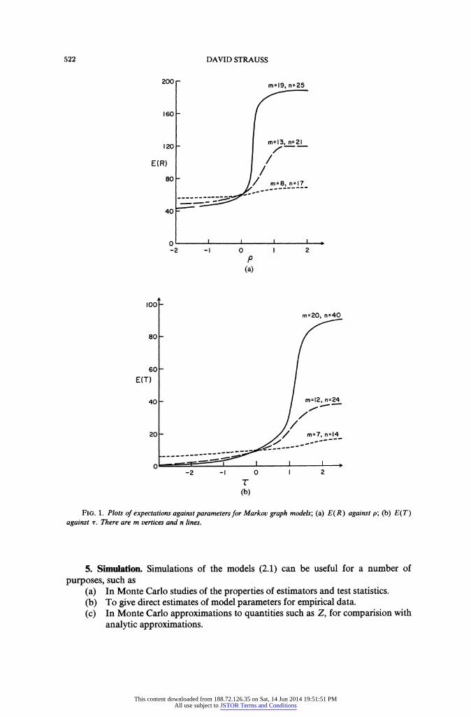
Figure l(a) illustrates the degeneracy. Each curve is the plot of the expectation of R against p. The curves were obtained by a simulation method to be described in the next section; the three pairs (m, n) were chosen so that in each case E(R) has the same value (60) when p = 0. Note that as (m, n) increase, the right derivative of E(R) at the origin increases. In the limit the derivative is singular at the origin.
For the random n case when p > 0 it is straightforward to verify (4.6), so that the model is degenerate. It can also be seen that whether n is fixed or random the model is proper when p < 0, which corresponds to repulsion between the lines.
4.3.4. The Markov graph transitivity model. The properties of the T-model (3.11) are very similar to those of the p-model. For simplicity, suppose n = (i), where k is an integer. When T> 0, the minimum energy configuration for n lines is a complete subgraph of k vertices. Thus Mn = (3), the number of distinct triads. Since Mn = 0(n 15), we again find that the model is degenerate in the nonrandom case, and also in the random case if ,u is chosen as in ?4.2. The nonrandom degeneracy can be interpreted as follows: if a graph has a positive transitivity tendency (however small), then as the number of lines increases the probability tends to one that an arbitrarily large fraction of the lines will coalesce into a clique. This is illustrated by Fig. l(b), which shows the same general features as Fig. l(a).
This content downloaded from 188.72.126.35 on Sat, 14 Jun 2014 19:51:51 PMAll use subject to JSTOR Terms and Conditions
FIG. 1. Plots of expectations against parameters for Markov graph models; (a) E(R) against p; (b) E(T) against r. There are m vertices and n lines.
5. Simulation. Simulations of the models (2.1) can be useful for a number of purposes, such as
(a) In Monte Carlo studies of the properties of estimators and test statistics. (b) To give direct estimates of model parameters for empirical data. (c) In Monte Carlo approximations to quantities such as Z, for comparision with
analytic approximations.
This content downloaded from 188.72.126.35 on Sat, 14 Jun 2014 19:51:51 PMAll use subject to JSTOR Terms and Conditions
Most practicable simulation methods for potential models are based on the Metropolis method (e.g. Hammersley and Handscomb (1964)). This generates a Markov chain on Q whose equilibrium probabilities are of the required form (2.1). The ap- proach has been developed in the statistical mechanics literature and has not been applied to systems such as graphs. For a review of the extensive applications to spatial and lattice schemes, see the articles in Berne (1977). In this section, we state a sim- plified version of the method and adapt it for the Markov graph models.
Take the state space S2 to be finite. For each Si E sa define a set S2 of neighbors of Si, with O c t2 and Si ?2. It is often convenient to set I 2il equal to a constant, N say, for all i. Write Pi for exp{ - U(S,)}/Z; note that PJ/Pj is known even if Z is not. Consider the Markov chain with transition probabilities
Pjl P(NPX) if Pj/Pi < 1 and j E: Sl,
(5.1) Pij 1/N if P/PiP1 and je:i2, c if j=i, 0 otherwise
where c is chosen so that Ejpij =1. It is known that provided that the chain is irreducible and aperiodic it has an equilibrium distribution with probabilities Pi.
We now apply this to the Markov graph model (3.10). Suppose that there -are m vertices and a fixed number n of edges (or occupied sites). We identify a realization S of the graph with its n edges. Choose any graph S1 and generate a sequence S1, S2, ... inductively as follows.
(1) At step k (> 1), pick at random an edge Ie Sk and another edge J $ Sk. The graph S' = Sk - I + J is a neighbor of Sk, obtained by changing one edge of Sk, and Sk, S' play the role of i,j in (5.1).
(2) Compute AR=R(Sk)-R(S'), where R is defined in (3.10). (3) If pAR?O set Skll=S'. If pAR>O, set Skll=S' with probability exp
(-pA R); otherwise set Sk+l = Sk- (4) Replace k by k+ 1 and return to (1).
The resulting Markov chain may be seen to have transition probabilities (5.1), with N=n{( )-n}. Further, it is irreducible and aperiodic. It follows that it has the required equilibrium distribution (3.10).
This method was used to obtain the curves in Fig. l(a). The procedure was (a) Pick a value of p. (b) Generate an initial configuration whose energy pR is near the minimum. (c) Perform a large number of steps of the simulation. (d) Average the values of R after discarding the first few hundred (this seems
sufficient to avoid the effect of the initial configuration). (e) Repeat for other values of p and fit a smooth curve.
Simulation of other models in the class (3.9) is entirely analogous to the above. The procedures may seem somewhat elaborate, but workable alternative methods
are not apparent. We note that these random graph simulations are much easier to implement than, for example, Metropolis simulations for spatial models. Most of the technical problems associated with the latter (Berne (1977)) do not arise. An exception is the estimation of Z: in both cases a simple unbiased estimator for Z1 is
1k D-nk Eexp{ U(Sj)),
1
This content downloaded from 188.72.126.35 on Sat, 14 Jun 2014 19:51:51 PMAll use subject to JSTOR Terms and Conditions
where the Si are realizations from the Markov chain in equilibrium, but such estimators are known to converge very slowly (Wood (1968)).
We conclude by illustrating how these simulations can be used to examine the properties of estimators. For the model (3.10) the maximum likelihood estimator of p satisfies
r=dK( p)
where r is the observed value of R and K(*) is its cumulant generating function when p = 0. Write the null cumulants as K1, K2,... as usual. If p is sufficiently small, we obtain a linear approximation to p
r- Kl (5.2) - K2
The expected bias of the estimator can be shown graphically as in Fig. 2. The curve is the plot of E(R) against p with m = 19 and n = 25, from Fig. 1(a). The oblique line is the tangent to the curve at p = 0. It can be seen that the expected proportional bias E(A - p)/p is given by the ratio AB: BC. Evidently p is seriously biased except when p is small.
We note that p could alternatively be used as a test statistic for the null hypothesis of randomness (p = 0).
6. Series expansions for the normalizing constant. 6.1. General considerations. It is usually necessary to know the constant Z in
(2.2), at least approximately, to estimate model parameters or to compare the fit of different models. The constant can always be estimated by Monte Carlo simulation, but this may be cumbersome for practical applications. An alternative is to develop a power series for Z or ln Z, the latter generally being the more convenient. The expansion may be in powers of any sufficiently small model parameter. There is an extensive literature on applications to statistical mechanics (a major reference being the volumes edited by Domb and Green (1974)), but the methods developed there have yet to be explored in other fields.
E(R)
-'C
0 p
FIG. 2. Bias of an estimator for the p-model. For each p the expected proportional bias in AB: BC.
This content downloaded from 188.72.126.35 on Sat, 14 Jun 2014 19:51:51 PMAll use subject to JSTOR Terms and Conditions
We indicate two general types of expansion. (a) Low intensity expansion. In many applications the potential function has a
natural scaling factor specifying intensity of interaction. In (3.3) this is the parameter v. Since Z is proportional to the expectation with respect to 1i of exp(- U) the expansion of ln Z in powers of v is just the null cumulant expansion of U with argument - v. This approach has been used by Strauss (1975), (1977); it leads to "truncated" estima- tors such as A in (5.2).
(b) Low density expansions. As an example, consider the square lattice model (3.8) with n sites occupied, V- n empty, and N occupied nearest neighbor pairs:
(6.1) P(S)=exp(na+Nfi)/Z(a,fi).
If a is large and negative the density n/V will be small. Set y = e and x = e- 2A. It can be shown that, as V-k oo, (1/V)lnZ tends to
1 ~00
(6.2) - - ln(xy)+ E y rg(x) 2r=1
where the gr are polynomials, the first 18 of which are tabulated by Domb (1974). Approximate maximum likelihood estimators for a,,f may readily be obtained from (6.1) and (6.2) and could, for example, be compared with those from the coding methods of Besag (1974).
We note that when a = 0 the limit of V- 1 In Z is known in closed form: this is the classic Onsager solution (Baxter (1982, p. 110)), one of the few cases where Z is known explicitly.
6.2. A spatial model for colored points under "sparseness." We conclude by apply- ing a low density expansion to obtain results for the colored spatial model with square-well potential (3.3). We begin with the one-color case. Let there be n points in a space of volume V. If n, V-- oo such that 4 = n/V is constant, it is known that
(6.3) lim -InZ= E Y,k
where the Yk are irreducible cluster integrals (Domb (1974)). Equation (6.3) is a cluster or virial expansion. Kubo (1962) gives a relatively short derivation. For a stable potential such as the square-well it is known that (6.3) has a positive radius of convergence.
The sparseness condition introduced by Saunders and Funk (1977) requires that X = n2/V remains constant as n, V-- oo and that boundary effects are asymptotically negligible. This implies that we may neglect all powers beyond the first in (6.3). Thus we have
lnZ= 1y1X.
The first cluster integral y1 is
JD [exp {-u (r12) }-1] dr12
For the square-well potential in two dimensions this is
This content downloaded from 188.72.126.35 on Sat, 14 Jun 2014 19:51:51 PMAll use subject to JSTOR Terms and Conditions
It can be shown that in the case of colored points there is a modified virial expansion in which Y1 is replaced by its expectation over the coloring distribution prescribed by ,i. We take ,u such that for each n the numbers of points of color c are multinomially distributed with parameters n and { Oc: cE C ). Let the pair-potential for colors c, d be
dr ( if O<r<Rcdg (6.4) ucd(r) - vcd cf Ecd _rRcd'
0 O otherwise
with ecd> 0. For any configuration Sn write
Ycd Ycdn(7Sn) = (S [ ) cd[ rid j < R cd]e
the sum being over pairs (i,j) with colors c, d. Thus Yc(n) is the number of interacting pairs of color c,d. To indicate dependence on n and v = { Vcd } in (6.4), we write the partition function as Z*(n, v). The joint cumulant generating function for the Yc(n) can be expressed as
K(n)(t) = lnZ*(n, t+ v) -lnZ*(n, v)
where t denotes {tcd }. Hence K(n)(t) converges to
where E indicates expectation with respect to colorings. Thus
(6.5) K (t) = 1XT E OCOd eXp vcd (exptcd- 1)(R d-ed). c,deC
Equation (6.5) asserts that as n - oo the Yc7n) converge to independent Poisson variables with means mcdexp(Vcd) where
12 mCd=2X'rO Od(R d-e.2 mCd = 2 Atc@ (RCd Ecd)
is the mean of YCd in the null case. Thus the only effect of the interaction on the counts YCd is to inflate the means of their null (Poisson) distribution independently by factors exp(vcd). It can also be seen that the sufficient statistics for the triples (Ecd,Rcd'Vcd) are independent, so that inference for each color pair may be performed independently. Thus if the sparseness condition holds, estimation and hypothesis testing for the clustering parameters becomes straightforward.
This rather simple derivation illustrates the power of the cluster expansion. For example, in the one color case and in the absence of all interactions, the result reduces to Theorem 1 of Saunders and Funk (1977), and their Theorem 2 can be rapidly obtained if (6.4) is replaced by a suitable step function. The original proofs were lengthy.
REFERENCES
R. J. BAXTER, Exactly Solved Models in Statistical Mechanics, Academic Press, London, 1982. J. E. BESAG, Spatial interaction and the statistical analysis of lattice systems (with discussion), J. Roy. Stat. Soc.
B, 36 (1974), pp. 192-236. B. BERNE, ed., Statistical Mechanics. Part A: Equilibrium Techniques, Plenum Press, New York, 1977. C. DoMB, Ising model, in Phase Transitions and Critical Pheonomena, Vol. 3, C. Domb and M. S. Green,
eds., Academic Press, London, 1974, pp. 357-784.
This content downloaded from 188.72.126.35 on Sat, 14 Jun 2014 19:51:51 PMAll use subject to JSTOR Terms and Conditions
C. DOMB AND M. S. GREEN, Phase transitions and critical phenomena, Vols. 1 and 3, Academic Press, London, 1974.
O. FRANK AND D. J. STRAUSS, Markov graphs, J. Amer. Statist. Assoc., 1986, to appear. D. J. GATES AND M. WESTCOTT, Clustering estimates in spatial point processes with unstable potentials,
unpublished, 1982. R. B. GRIFFITHS, Rigorous results and theorems, in Phase Transitions and Critical Phenomena, Vol. 1, C.
Domb and M. S. Green, eds., Academic Press, London, 1972, pp. 7-109. J. M. HAMMERSLEY AND D. C. HANDSCOMB, Monte Carlo Methods, Methuen, London, 1964. E. T. JAYNES, Where do we stand on maximum entropy? in The Maximum Entropy Formalism, E. Levine and
M. Tribus, eds., MIT Press, Cambridge, MA, 1978, pp. 15-118. F. P. KELLY AND B. D. RIPLEY, A note on Strauss' modelfor clustering, Biometrika, 63 (1976), pp. 357-360. R. KUBO, Generalized cumulant expansion method, J. Phys. Soc. Japan, 17 (1962), pp. 1100-1120. R. J. KRYScIo, R. SAUNDERS AND G. M. FUNK, Normal approximations for binary lattice systems, J. Appl.
Prob., 17 (1980), pp. 674-685. Y. OGATA AND M. TANEMURA, Estimation of interaction potentials of spatial point patterns through the
maximum likelihoodprocedure, Ann. Inst. Stat. Math., 33 (1981), pp. 315-338. , Likelihood analysis of spatialpoint patterns, J. Roy. Stat. Soc. B, 46 (1984), pp. 496-518.
D. K. PicKARD, Asymptotic inference for an Ising lattice. II, Adv. Appl. Prob., 9, (1977), pp. 476-501. B. D. RIPLEY, Modelling spatialpatterns (with discussion), J. Roy. Stat. Soc. B, 39 (1977), pp. 172-212.
, Spatial Statistics, New York, John Wiley, 1981. D. RUELLE, Statisical Mechanics: Rigorous Results, Benjamin, New York, 1969. R. SAUNDERS AND G. M. FUNK, Poisson limits for a clustering model of Strauss, J. Appl. Prob., 14 (1977), pp.
776-784. R. SAUNDERS, R. J. KRYSCIO AND G. M. FuNK, Limiting results for arrays of binary random variables on
rectangular lattices under sparseness conditions, J. Appl. Prob., 16, (1979), pp. 554-566. , Poisson limits for a hard core clustering model, Stoch. Proc. Appl., 12 (1982), pp. 97-106.
D. J. STRAUSS, A modelfor clustering, Biometrika, 62 (1975), pp. 467-475. , Clustering on colored lattices, J. Appl. Prob., 14 (1977), pp. 135-143.
W. W. WOOD, Monte Carlo studies of simple liquid models, Physics of Simple Liquids, H. N. V. Temperley et al., eds., North-Holland, Amsterdam, 1968, pp. 115-230.
This content downloaded from 188.72.126.35 on Sat, 14 Jun 2014 19:51:51 PMAll use subject to JSTOR Terms and Conditions