Page 1
ON A HARDY TYPE INEQUALITY AND ASINGULAR STURM-LIOUVILLE EQUATION
BY HUI WANG
A dissertation submitted to the
Graduate School—New Brunswick
Rutgers, The State University of New Jersey
in partial fulfillment of the requirements
for the degree of
Doctor of Philosophy
Graduate Program in Mathematics
Written under the direction of
Haim Brezis
and approved by
New Brunswick, New Jersey
January, 2014
Page 2
c© 2014
Hui Wang
ALL RIGHTS RESERVED
Page 3
ABSTRACT OF THE DISSERTATION
On a Hardy type inequality and a singular
Sturm-Liouville equation
by Hui Wang
Dissertation Director: Haim Brezis
In this dissertation, we first prove a Hardy type inequality for u ∈ Wm,10 (Ω), where
Ω is a bounded smooth domain in RN and m ≥ 2. For all j ≥ 0, 1 ≤ k ≤ m − 1,
such that 1 ≤ j + k ≤ m, it holds that ∂ju(x)d(x)m−j−k ∈ W k,1
0 (Ω), where d is a smooth
positive function which coincides with dist(x, ∂Ω) near ∂Ω, and ∂l denotes any partial
differential operator of order l.
We also study a singular Sturm-Liouville equation −(x2αu′)′ + u = f on (0, 1),
with the boundary condition u(1) = 0. Here α > 0 and f ∈ L2(0, 1). We prescribe
appropriate (weighted) homogeneous and non-homogeneous boundary conditions at 0
and prove the existence and uniqueness of H2loc(0, 1] solutions. We study the regularity
at the origin of such solutions. We perform a spectral analysis of the differential operator
Lu := −(x2αu′)′ + u under homogeneous boundary conditions.
Finally, we are interested in the equation −(|x|2αu′)′ + |u|p−1u = µ on (−1, 1) with
boundary condition u(−1) = u(1) = 0. Here α > 0, p ≥ 1 and µ is a bounded Radon
measure on the interval (−1, 1). We identify an appropriate concept of solution for
this equation, and we establish some existence and uniqueness results. We examine the
limiting behavior of three approximation schemes. The isolated singularity at 0 is also
investigated.
ii
Page 4
Preface
This dissertation is a compilation of the research papers written by the author during
the course of his Ph. D. Each chapter in this dissertation contains one paper, while the
references are collected at the end of this dissertation. Minor changes are made from
the original papers in order to keep the consistency of the presentation style. Some
chapters are collaborative work (with H. Castro for Chapter 1, 3 and 4, and with H.
Castro and J. Davlia for Chapter 2). Chapter 5 and 6 are written solely by the author.
iii
Page 5
Acknowledgements
I would like to express my deepest gratitude to my thesis advisor Professor Haim Brezis
for his continuous guidance, encouragement and support, and for providing me the
invaluable opportunities to interact with mathematicians around the world. It is my
privilege and my most exciting experience to work with him. His insight and enthusiasm
of mathematics has greatly inspired me.
I would like to thank Professors S. Chanillo, Z.-C. Han, X. Huang, Y.Y. Li, R.
Nussbaum, J. Song for their wonderful courses and for their enlightening discussions
throughout my graduate study. I would like to thank Professor L. Veron for the exten-
sive and effective discussions and for his long-lasting help. I would also like to thank
Professor J. Davila for his collaboration. I want to thank Professor P. Mironescu for
many interesting discussions. I wish to thank Professors Y. Almog, M. Marcus, E.
Milman, Y. Pinchover, S. Reich, J. Rubinstein, I. Shafrir, G. Wolansky for their help
during my stay at the Technion. I also owe my thanks to Professors H. Sussmann and
G. Wang for their help in the beginning of my graduate study.
I wish to thank my collaborator and friend Hernan Castro. Thank him for the great
discussions that lead to several joint papers. I am also grateful for all my friends at
Rutgers and the Technion. Thank all of them to make my life enjoyable.
I am gratitude for the financial support by the Department of Mathematics at Rut-
gers and by the ITN “FIRST” of the Seventh Framework Programme of the European
Community (grant agreement number 238702).
Last but not least, I am indebted to my family for always being supportive and for
their encouragement that keeps me going.
iv
Page 6
Table of Contents
Abstract . . . . . . . . . . . . . . . . . . . . . . . . . . . . . . . . . . . . . . . . ii
Preface . . . . . . . . . . . . . . . . . . . . . . . . . . . . . . . . . . . . . . . . . iii
Acknowledgements . . . . . . . . . . . . . . . . . . . . . . . . . . . . . . . . . iv
1. A Hardy type inequality for Wm,1(0,1) functions (written with H. Castro,
Car. Val. Partial Differential Equations, 39 (2010), 525–531) . . . . . . . . . . . 1
1.1. Introduction . . . . . . . . . . . . . . . . . . . . . . . . . . . . . . . . . . 1
1.2. Proof of Theorem 1.2 . . . . . . . . . . . . . . . . . . . . . . . . . . . . . 2
1.3. The Wm,p functions with m ≥ 2 and p > 1 . . . . . . . . . . . . . . . . . 5
2. A Hardy type inequality for Wm,10 (Ω) functions (written with H. Castro
and J. Davila, C. R. Acad. Sci. Paris, Ser. I 349 (2011), 765–767, detailed version
in J. Eur. Math. Soc. 15 (2013), 145–155) . . . . . . . . . . . . . . . . . . . . . 7
2.1. Introduction . . . . . . . . . . . . . . . . . . . . . . . . . . . . . . . . . . 7
2.2. Notation and preliminaries . . . . . . . . . . . . . . . . . . . . . . . . . 8
2.3. The case m = 2 . . . . . . . . . . . . . . . . . . . . . . . . . . . . . . . . 11
2.4. The general case m ≥ 2 . . . . . . . . . . . . . . . . . . . . . . . . . . . 15
3. A singular Sturm-Liouville equation under homogeneous boundary
conditions (written with H. Castro, J. Funct. Anal. 261 (2011), 1542–1590) . . 18
3.1. Introduction . . . . . . . . . . . . . . . . . . . . . . . . . . . . . . . . . . 18
3.1.1. The case 0 < α < 12 . . . . . . . . . . . . . . . . . . . . . . . . . 19
3.1.2. The case 12 ≤ α < 3
4 . . . . . . . . . . . . . . . . . . . . . . . . . 23
3.1.3. The case 34 ≤ α < 1 . . . . . . . . . . . . . . . . . . . . . . . . . 25
3.1.4. The case α ≥ 1 . . . . . . . . . . . . . . . . . . . . . . . . . . . . 26
v
Page 7
3.1.5. Connection with the variational formulation . . . . . . . . . . . . 28
3.1.6. The spectrum . . . . . . . . . . . . . . . . . . . . . . . . . . . . . 29
3.2. Proofs of all the uniqueness results . . . . . . . . . . . . . . . . . . . . . 32
3.3. Proofs of all the existence and the regularity results . . . . . . . . . . . 38
3.3.1. The Dirichlet problem . . . . . . . . . . . . . . . . . . . . . . . . 39
3.3.2. The Neumann problem and the “Canonical” problem . . . . . . 42
3.4. The spectrum of the operator Tα . . . . . . . . . . . . . . . . . . . . . . 51
3.4.1. The eigenvalue problem for all α > 0 . . . . . . . . . . . . . . . . 51
3.4.2. The rest of the spectrum for the case α ≥ 1 . . . . . . . . . . . . 57
3.4.3. The proof of Theorem 3.19 . . . . . . . . . . . . . . . . . . . . . 60
3.5. The spectrum of the operator TD . . . . . . . . . . . . . . . . . . . . . . 62
3.6. Appendix: a weighted Sobolev space . . . . . . . . . . . . . . . . . . . . 62
4. A singular Sturm-Liouville equation under non-homogeneous bound-
ary conditions, (written with H. Castro, Differential Integral Equations 25 (2012),
85–92) . . . . . . . . . . . . . . . . . . . . . . . . . . . . . . . . . . . . . . . . . . 71
4.1. Introduction . . . . . . . . . . . . . . . . . . . . . . . . . . . . . . . . . . 71
4.2. Proof of the theorems . . . . . . . . . . . . . . . . . . . . . . . . . . . . 72
5. A singular Sturm-Liouville equation involving measure data (Commun.
Contemp. Math 15 (2013)) . . . . . . . . . . . . . . . . . . . . . . . . . . . . . . 78
5.1. Introduction . . . . . . . . . . . . . . . . . . . . . . . . . . . . . . . . . . 78
5.2. An unbounded operator on L1(−1, 1) . . . . . . . . . . . . . . . . . . . . 83
5.3. Non-uniqueness when 0 < α < 1 . . . . . . . . . . . . . . . . . . . . . . 91
5.4. Proof of the existence results . . . . . . . . . . . . . . . . . . . . . . . . 93
5.5. The elliptic regularization . . . . . . . . . . . . . . . . . . . . . . . . . . 98
5.6. The lack of stability of the good solution when 12 ≤ α < 1 . . . . . . . . 108
5.7. The problem on the interval (0, 1) . . . . . . . . . . . . . . . . . . . . . 117
vi
Page 8
6. A semilinear singular Sturm-Liouville equation involving measure data
(to appear at Ann. Inst. H. Poincare Anal. Non Lineaire) . . . . . . . . . . . . . 122
6.1. Introduction . . . . . . . . . . . . . . . . . . . . . . . . . . . . . . . . . . 122
6.2. Proof of the uniqueness and existence results . . . . . . . . . . . . . . . 128
6.3. The elliptic regularization . . . . . . . . . . . . . . . . . . . . . . . . . . 135
6.4. The approximation via truncation . . . . . . . . . . . . . . . . . . . . . 140
6.5. The lack of stability of the good solution for 12 ≤ α < 1 and 1 < p < 1
2α−1 146
6.6. The non-uniqueness for the case (6.3) and (6.4) . . . . . . . . . . . . . . 148
6.7. Removable singularity . . . . . . . . . . . . . . . . . . . . . . . . . . . . 150
6.8. Classification of the singularity . . . . . . . . . . . . . . . . . . . . . . . 155
6.9. The equation on the interval (0, 1) . . . . . . . . . . . . . . . . . . . . . 165
References . . . . . . . . . . . . . . . . . . . . . . . . . . . . . . . . . . . . . . . 174
vii
Page 9
1
Chapter 1
A Hardy type inequality for Wm,1(0,1) functions
1.1 Introduction
It is well known ([31]) that if u ∈ W 1,p(0, 1) and u(0) = 0 then the Hardy inequality
holds for p > 1, that is∫ 1
0
∣∣∣∣u(x)x∣∣∣∣p dx ≤ ( p
p− 1
)p ∫ 1
0
∣∣u′(x)∣∣p dx.The constant p
p−1 is optimal for this inequality and it blows up as p goes to 1. This
behaviour is confirmed by the fact that no such inequality can be proved when p = 1,
as we can consider (see e.g. [8]) the non-negative function on (0, 1) defined by
v(x) =1
1− log x. (1.1)
A simple computation shows that this function belongs to W 1,1(0, 1), u(0) = 0, but u(x)x
is not integrable.
When we turn to functions u ∈ W 2,p(0, 1), p ≥ 1, with u(0) = u′(0) = 0, there are
three natural quantities to consider: u(x)x2 ,
u′(x)x and
(u(x)
x
)′= u′(x)
x − u(x)x2 . If p > 1,
it is clear that both u′(x)x and u(x)
x2 = u′(x)x − 1
x2
∫ x0 tu
′′(t)dt belong to Lp(0, 1). Thus(u(x)
x
)′∈ Lp(0, 1). If p = 1 one can no longer assert that u(x)
x2 ,u′(x)
x belong to L1(0, 1),
but surprisingly(
u(x)x
)′∈ L1(0, 1). This reflects a “magic” cancellation of the non-
integrable terms in the difference(
u(x)x
)′= u′(x)
x − u(x)x2 .
The same phenomenon remains valid when we keep increasing the number of deriva-
tives, and this is the main result of this chapter.
Definition 1.1. We say that u has the property (Pm) if
u ∈Wm,1(0, 1) and u(0) = Du(0) = . . . = Dm−1u(0) = 0,
where Diu denotes the i-th derivative of u.
Page 10
2
Theorem 1.2. Assume u has the property (Pm) and j, k are non-negative integers.
(i) If k ≥ 1 and 1 ≤ j + k ≤ m, then Dju(x)xm−j−k has the property (Pk) and∥∥∥∥Dk
(Dju(x)xm−j−k
)∥∥∥∥L1(0,1)
≤ (k − 1)!(m− j − 1)!
‖Dmu‖L1(0,1) . (1.2)
The constant is optimal.
(ii) There exists w having the property (Pm) such that
Djw(x)xm−j
/∈ L1(0, 1), ∀j = 0, . . . ,m− 1. (1.3)
Remark 1.1. For functions u ∈ W 2,p(0, 1), p > 1, with u(0) = u′(0) = 0, a slightly
stronger result holds, namely, when we estimate the Lp norms of the three quantitiesu(x)x2 ,
u′(x)x and
(u(x)
x
)′, we obtain∥∥∥∥u(x)x2
∥∥∥∥p
≤ αp
∥∥u′′∥∥p,
∥∥∥∥u′(x)x
∥∥∥∥p
≤ βp
∥∥u′′∥∥p, and
∥∥∥∥(u(x)x)′∥∥∥∥
p
≤ γp
∥∥u′′∥∥p, (1.4)
with αp, βp, γp as the best possible constants. It is easy to see that αp → ∞, βp → ∞
when p→ 1. However, a similar “magic” cancellation appears and γp remains bounded
as p→ 1. A proof of this latter fact is presented in Section 1.3.
1.2 Proof of Theorem 1.2
We begin with the following observation.
Lemma 1.3 (Representation formula). If u has property (Pm), then
u(x) =1
(m− 1)!
∫ x
0Dmu(s)(x− s)m−1ds.
Proof. We proceed by induction. The case m = 1 is immediate since u ∈ W 1,1(0, 1) if
and only if u is absolutely continuous. Now notice that
Dm−1u(x) =∫ x
0Dmu(s)ds.
If we use the induction hypothesis, we obtain
u(x) =1
(m− 2)!
∫ x
0
(∫ s
0Dmu(t)dt
)(x− s)m−2ds.
The proof is completed after using Fubini’s Theorem.
Page 11
3
Based on the function defined by (1.1), we have
Lemma 1.4. There exists a function w having property (Pm), such that
Dm−1w(x)x
,Dm−2w(x)
x2, . . . ,
Dw(x)xm−1
,w(x)xm
/∈ L1. (1.5)
Proof. In order to construct the function w, we consider the function v defined in (1.1).
As we said, v is a non-negative function on (0, 1), it has the property (P1), but v(x)x
does not belong to L1(0, 1). Define w(x) as
w(x) =1
(m− 2)!
∫ x
0v(s)(x− s)m−2ds,
so w solves the equation Dm−1w(x) = v(x), with initial condition w(0) = Dw(0) =
. . . = Dm−2w(0) = 0. Notice that w has the property (Pm), Dkw(x) ≥ 0, Dkw(1) <∞
and
lims→0
Dm−kw(s)sk−1
= 0,
for all k = 1, . . . ,m− 1. We now show that w satisfies (1.5). Notice that
+∞ =∫ 1
0
v(x)x
dx
=∫ 1
0
Dm−1w(x)x
dx
= Dm−2w(1) +∫ 1
0
Dm−2w(x)x2
dx.
Thus∫ 10
Dm−2w(x)x2 dx = +∞. Similarly, if we keep integrating by parts we conclude that∥∥∥∥Dm−jw(x)
xj
∥∥∥∥L1(0,1)
=∫ 1
0
Dm−jw(x)xj
= ∞, ∀ j = 1, . . . ,m.
We can proceed to the
Proof of Theorem 1.2. The second part was proved in Lemma 1.4, so we will only prove
the first part. Since the result is immediate when j+k = m, in the following we always
assume that j + k ≤ m− 1.
To prove that Dju(x)xm−j−k has the property (Pk), we proceed by induction. For k = 1
and any j = 0, . . . ,m− 1, Dju(x)xm−j−1 has the property (P1) because
Dju(x)xm−j−1
∣∣∣∣x=0
= (m− j − 1)!Dm−1u(0) = 0.
Page 12
4
Now assume the result holds for some k. Notice that if j + k + 1 ≤ m− 1 then
D
(Dju(x)xm−j−k−1
)=
Dj+1u(x)xm−(j+1)−k
− (m− j − k − 1)Dju(x)xm−j−k
,
the righthand side of which has property (Pk) by the induction assumption. Thus we
conclude that D(
Dju(x)xm−j−k−1
)has the property (Pk), completing the induction step.
Now we prove the estimate (1.2). Notice that
Dk
(Dju(x)xm−j−k
)=
k∑i=0
(k
i
)Dj+iu(x)Dk−i
(1
xm−j−k
), (1.6)
and that
Dk−i
(1
xm−j−k
)= (−1)k−i (m− j − i− 1)!
(m− j − k − 1)!1
xm−j−i. (1.7)
Using the representation formula for u from Lemma 1.3, we obtain
Di+ju(x) =1
(m− j − i− 1)!
∫ x
0Dmu(s)(x− s)m−j−i−1ds. (1.8)
By combining (1.6), (1.7) and (1.8) we obtain
Dk
(Dju(x)xm−j−k
)=
k∑i=0
z(−1)k−i 1(m− j − k − 1)!
∫ x
0Dmu(s)
(x− s)m−j−i−1
xm−j−ids
=1
(m− j − k − 1)!
∫ x
0Dmu(s)
(x− s)m−j−1
xm−j
(k∑
i=0
(k
i
)(x
x− s
)i
(−1)k−i
)ds
=1
(m− j − k − 1)!
∫ x
0Dmu(s)
(x− s)m−j−1
xm−j
(s
x− s
)k
ds.
=1
(m− j − k − 1)!
∫ x
0Dmu(s)
(1− s
x
)m−j−k−1 ( sx
)k−1 s
x2ds.
Therefore,∫ 1
0
∣∣∣∣Dk
(Dju(x)xm−j−k
)∣∣∣∣ dx≤ 1
(m− j − k − 1)!
∫ 1
0|Dmu(s)|
(∫ 1
s
(1− s
x
)m−j−k−1 ( sx
)k−1 s
x2dx
)ds
=1
(m− j − k − 1)!
∫ 1
0|Dmu(s)|
(∫ 1
s(1− t)m−j−k−1 tk−1dt
)ds
≤ 1(m− j − k − 1)!
‖Dmu‖L1(0,1)
∫ 1
0(1− t)m−j−k−1 tk−1dt
=(k − 1)!
(m− j − 1)!‖Dmu‖L1(0,1) .
Page 13
5
The optimality of the constant is guaranteed by the optimality of Holder’s inequality.
The proof of the theorem is now completed.
1.3 The Wm,p functions with m ≥ 2 and p > 1
We begin by proving the result stated in Remark 1.1. Notice that for u ∈ W 2,p(0, 1)
satisfying u(0) = u′(0) = 0, we can write(u(x)x
)′=
1x2
∫ x
0su′′(s)ds.
For p > 1, we can apply Holder’s inequality and Fubini’s theorem to obtain,∫ 1
0
∣∣∣∣(u(x)x)′∣∣∣∣p dx ≤ ∫ 1
0
xpp′
x2p
∫ x
0sp∣∣u′′(s)∣∣p dsdx
=∫ 1
0sp∣∣u′′(s)∣∣p(∫ 1
s
1xp+1
dx
)ds
≤ 1p
∫ 1
0
∣∣u′′(s)∣∣p ds,where p′ and p are given by 1
p + 1p′ = 1. Hence∥∥∥∥(u(x)x
)′∥∥∥∥p
≤ p− 1
p∥∥u′′∥∥
p.
Thus, if we define γp as in (1.4), we have proved that γp ≤ p− 1
p , i.e., γp remains bounded
as p→ 1.
As one might expect, an analogue to Theorem 1.2 can be proved for Wm,p functions.
The result reads as follows
Theorem 1.5. Let m ≥ 2 and p > 1. If u belongs to Wm,p(0, 1) and satisfies u(0) =
Du(0) = . . . = Dm−1u(0) = 0, then for k ≥ 1 and 1 ≤ j + k ≤ m,∥∥∥∥Dk
(Dju(x)xm−j−k
)∥∥∥∥Lp(0,1)
≤ B(pk, p(m− j − k − 1) + 1)1p
(m− j − k − 1)!‖Dmu‖Lp(0,1) , (1.9)
where B(a, b) =∫ 10 t
a−1(1− t)b−1dt denotes Euler’s Beta function.
Proof. From the proof of Theorem 1.2, we have
Dk
(Dju(x)xm−j−k
)=
1(m− j − k − 1)!
∫ x
0Dmu(s)
(1− s
x
)m−j−k−1 ( sx
)k−1 s
x2ds.
Page 14
6
After applying Holder’s inequality, Fubini’s theorem and a change of variables one
obtains that∫ 1
0
∣∣∣∣Dk
(Dju(x)xm−j−k
)∣∣∣∣p dx≤(
1(m− j − k − 1)!
)p ∫ 1
0|Dmu(s)|p
(∫ 1
s(1− t)p(m−j−k−1) tpk−1dt
)ds
≤(
1(m− j − k − 1)!
)p ∫ 1
0|Dmu(s)|p
(∫ 1
0(1− t)p(m−j−k−1) tpk−1dt
)ds
=B(pk, p(m− j − k − 1) + 1)(
1(m− j − k − 1)!
)p ∫ 1
0|Dmu(s)|p ds.
Page 15
7
Chapter 2
A Hardy type inequality for Wm,10 (Ω) functions
2.1 Introduction
In this chapter, we prove the following result, which is the higher dimensional analogue
of the Theorem 1.2 in Chapter 1.
Theorem 2.1. Let Ω be a bounded domain in RN with smooth boundary ∂Ω. Given
x ∈ Ω, we denote by δ(x) the distance from x to the boundary ∂Ω. Let d : Ω → (0,+∞)
be a smooth function such that d(x) = δ(x) near ∂Ω. Suppose m ≥ 2 and let j, k be
non-negative integers such that 1 ≤ k ≤ m − 1 and 1 ≤ j + k ≤ m. Then for every
u ∈Wm,10 (Ω), we have ∂ju(x)
d(x)m−j−k ∈W k,10 (Ω) with∥∥∥∥∂k
(∂ju(x)
d(x)m−j−k
)∥∥∥∥L1(Ω)
≤ C ‖u‖W m,1(Ω) , (2.1)
where ∂l denotes any partial differential operator of order l and C > 0 is a constant
depending only on Ω and m.
Remark 2.1. We will see that the proof of Theorem 2.1 is different from the proof of
Theorem 1.2 if we consider, for example, N = 2, Ω = R2+ = (x1, x2); x2 ≥ 0, x1 ∈ R,
and u ∈ C∞c ([0, 1]× [0, 1]). From Theorem 1.2 it is clear that∫Ω
∣∣∣∣ ∂∂x2
(u(x1, x2)
x2
)∣∣∣∣ dx1dx2 ≤ C
∫Ω
∣∣∣∣∂2u(x1, x2)∂x2
2
∣∣∣∣ dx1dx2.
However new technique (Lemma 2.6) will be needed to derive∫Ω
∣∣∣∣ ∂∂x1
(u(x1, x2)
x2
)∣∣∣∣ dx1dx2 ≤ C∥∥D2u
∥∥L1(Ω)
.
The rest of this chapter is organized as the following. In Section 2.2 we introduce
the notation used throughout this chapter and give some preliminary results. In order
Page 16
8
to present the main ideas used to prove Theorem 2.1, we begin in Section 2.3 with the
proof of Theorem 2.1 for the special case m = 2. Then in Section 2.4 we provide the
proof of Theorem 2.1 for the general case m ≥ 2.
2.2 Notation and preliminaries
Throughout this work, we denote RN+ =
(y1, . . . , yN−1, yN ) ∈ RN ; yN > 0
, the upper
half space, and BNr (x0) =
x ∈ RN ; |x− x0| < r
. When x0 = 0, we write BN
r =
BNr (0).
Let Ω be a bounded domain in RN with smooth boundary ∂Ω. Given x ∈ Ω, we
denote by δ(x) the distance from x to the boundary ∂Ω, that is
δ(x) = dist(x, ∂Ω) = inf |x− y| ; y ∈ ∂Ω .
For ε > 0, the tubular neighborhood of ∂Ω in Ω is the set
Ωε = x ∈ Ω; δ(x) < ε .
The following is a well known result (see e.g. Lemma 14.16 in [30]) and it shows that
δ is smooth in some neighborhood of ∂Ω.
Lemma 2.2. Let Ω and δ : Ω → (0,∞) be as above. Then there exists ε0 > 0 only
depending on Ω, such that δ|Ωε0: Ωε0 → (0,∞) is smooth. Moreover, for every x ∈ Ωε0
there exists a unique yx ∈ ∂Ω so that
x = yx + δ(x)ν∂Ω(yx),
where ν∂Ω denotes the unit inward normal vector field associated to ∂Ω.
Since ∂Ω is smooth, for fixed x0 ∈ ∂Ω, there exists a neighborhood V(x0) ⊂ ∂Ω, a
radius r > 0 and a map
Φ : BN−1r → V(x0) (2.2)
which defines a smooth diffeomorphism. Define
N+(x0) = x ∈ Ωε0 ; yx ∈ V(x0) , (2.3)
Page 17
9
where ε0 and yx are given in Lemma 2.2. We define Φ : BN−1r × (−ε0, ε0) → RN as
Φ(y, t) = Φ(y) + yN · ν∂Ω(Φ(y)), (2.4)
where y = (y1, . . . , yN−1), and we write
N (x0) = Φ(BN−1
r × (−ε0, ε0)). (2.5)
About the map Φ we have the following
Lemma 2.3. The map Φ|BN−1r ×(0,ε0) is a diffeomorphism and
N+(x0) = Φ(BN−1
r × (0, ε0)).
Proof. This is a direct corollary of the definition of Φ through Φ, and Lemma 2.2.
Remark 2.2. The map Φ|BN−1r ×(0,ε0) gives a local coordinate chart which straightens
the boundary near x0. This type of coordinates are sometimes called flow coordinates
(see e.g. [9] and [33]).
From now on, C > 0 will always denote a constant only depending on Ω and possibly
the integer m ≥ 2. The following is a direct, but very useful, corollary.
Corollary 2.4. Let f ∈ L1(N+(x0)) and Φ be given by (2.4). Then
1C
∫BN−1
r
∫ ε0
0|f(Φ(y, yN ))| dyNdy ≤
∫N+(x0)
|f(x)| dx
≤C∫
BN−1r
∫ ε0
0|f(Φ(y, yN ))| dyNdy
Proof. Since Φ|BN−1r ×(0,ε0) is a diffeomorphism, we know that for all (y, yN ) ∈ BN−1
r ×
(0, ε0) we have1C≤ |detDΦ(y, yN )| ≤ C.
The result then follows from the change of variables formula.
The following lemma provides us a partition of unity in RN , constructed from the
neighborhoods N (x0). Consider the open cover of ∂Ω given by V(x); x ∈ ∂Ω, where
V(x) ⊂ ∂Ω is defined in (2.2). By the compactness of ∂Ω, there exists x1, . . . , xM ⊂
∂Ω, so that ∂Ω = ∪Ml=1V(xl). Notice that by the definition of N (x0) in (2.5) we also
Page 18
10
have that ∪Ml=1N (xl) is an open cover of ∂Ω in RN . The following is a classical result
(see e.g. Lemma 9.3 in [8] and Theorem 3.15 in [1]).
Lemma 2.5 (partition of unity). There exist functions ρ0, ρ1, . . . , ρM ∈ C∞(RN ) such
that
(i) 0 ≤ ρl ≤ 1 for all l = 0, 1, . . . ,M and∑M
l=0 ρi(x) = 1 for all x ∈ RN ,
(ii) supp ρl ⊂ N (xl), for all l = 1, . . . ,M ,
(iii) ρ0|Ω ∈ C∞c (Ω).
In order to simplify the notation, we will denote by ∂l any partial differential oper-
ator of order l where l is a positive integer1. Also, ∂i will denote the partial derivative
with respect to the i-th variable, and ∂2ij = ∂i ∂j .
Remark 2.3. We conclude this section by showing that, to prove Theorem 2.1, it
is enough to prove estimate (2.1) for smooth functions with compact support. Suppose
u ∈Wm,10 (Ω), then there exists a sequence un ⊂ C∞c (Ω), so that ‖u− un‖W m,1(Ω) → 0
as n→∞. In particular, after maybe extracting a subsequence, one can assume that
∂lun → ∂lu a.e. in Ω, for all 0 ≤ l ≤ m.
Since d is smooth, the above implies that for a.e. x ∈ Ω and all j ≥ 0, 1 ≤ k ≤ m− 1
and 1 ≤ j + k ≤ m:
∂k
(∂ju(x)
d(x)m−j−k
)=
∂j+ku(x)d(x)m−j−k
+ ∂ju(x)∂k
(1
d(x)m−j−k
)= lim
n→∞
∂j+kun(x)d(x)m−j−k
+ ∂jun(x)∂k
(1
d(x)m−j−k
)= lim
n→∞∂k
(∂jun(x)d(x)m−j−k
).
Therefore, Fatou’s Lemma applies and we obtain∥∥∥∥∂k
(∂ju(x)
d(x)m−j−k
)∥∥∥∥L1(Ω)
≤ lim infn→∞
∥∥∥∥∂k
(∂jun(x)d(x)m−j−k
)∥∥∥∥L1(Ω)
.
1In general, one would say: “For a given multi-index α = (α1, . . . , αN ), we denote by ∂α the partialdifferential operator of order l = |α| = α1 + . . . + αN”. Since we only care about the order of theoperator, it makes sense to abuse the notation and identify α with its order |α| = l.
Page 19
11
Once (2.1) were proved for un ∈ C∞c (Ω), we get∥∥∥∥∂k
(∂jun(x)d(x)m−j−k
)∥∥∥∥L1(Ω)
≤ C ‖un‖W m,1(Ω) ,
and thus we can conclude that∥∥∥∥∂k
(∂ju(x)
d(x)m−j−k
)∥∥∥∥L1(Ω)
≤ C lim infn→∞
‖un‖W m,1(Ω) = C ‖u‖W m,1(Ω) .
Finally, the fact that ∂jun(x)d(x)m−j−k ∈ C∞c (Ω) and C∞c (Ω)
W k,1(Ω)= W k,1
0 (Ω) gives that∂ju(x)
d(x)m−j−k ∈W k,10 (Ω).
2.3 The case m = 2
We begin this section by proving estimate (2.1) in Theorem 2.1 for Ω = RN+ , m = 2,
j = 0 and k = 1.
Lemma 2.6. Suppose that u ∈ C∞c (RN+ ). Then for all i = 1, . . . , N∥∥∥∥∂i
(u(y)yN
)∥∥∥∥L1(RN
+ )
≤ 2 ‖u‖W 2,1(RN+ ) .
Proof. Consider first the case i = N . The proof is essentially the same as (1.2), but for
the sake of completeness, we still provide the proof. Notice that we can write
∂
∂yN
(u(y, yN )yN
)=
1y2
N
∫ yN
0
∂2
∂y2N
u(y, t)tdt.
Then integration by parts yields that∫RN−1
∫ ∞
0
∣∣∣∣ ∂
∂yN
(u(y, yN )yN
)∣∣∣∣ dyNdy ≤∫
RN−1
∫ ∞
0
1y2
N
∫ yN
0
∣∣∣∣ ∂2
∂y2N
u(y, t)∣∣∣∣ tdtdyNdy
=∫
RN−1
∫ ∞
0
∣∣∣∣ ∂2
∂y2N
u(y, t)∣∣∣∣ t ∫ ∞
t
1y2
N
dyNdtdy
=∫
RN−1
∫ ∞
0
∣∣∣∣ ∂2
∂y2N
u(y, t)∣∣∣∣ t ∫ ∞
t
1y2
N
dyNdtdy
=∫
RN−1
∫ ∞
0
∣∣∣∣ ∂2
∂y2N
u(y, t)∣∣∣∣ dtdy.
Hence ∫RN
+
∣∣∣∣ ∂
∂yN
(u(y)yN
)∣∣∣∣ dy ≤ ∫RN
+
∣∣∣∣∂2u(y)∂y2
N
∣∣∣∣ dy. (2.6)
Page 20
12
When 1 ≤ i ≤ N − 1, we need to estimate∫
RN+
1yN
∣∣∣ ∂u∂yi
(y)∣∣∣ dy. To do so, consider
the change of variables y = Ψ(x), where
Ψ(x1, . . . , xi, . . . , xN ) = (x1, . . . , xi + xN , . . . , xN ). (2.7)
Notice that detDΨ(x) = 1, so∫RN
+
1yN
∣∣∣∣∂u(y)∂yi
∣∣∣∣ dy =∫
RN+
1xN
∣∣∣∣ ∂u∂yi(Ψ(x))
∣∣∣∣ dx.Observe that if we let v(x) = u(Ψ(x)), we can write
1xN
∂u
∂yi(Ψ(x)) =
∂
∂xN
(v(x)xN
)− ∂
∂yN
(u(y)yN
)∣∣∣∣y=Ψ(x)
. (2.8)
Applying estimate (2.6) to u and v yields∫RN
+
1xN
∣∣∣∣ ∂u∂yi(Ψ(x))
∣∣∣∣ dx ≤ ∫RN
+
∣∣∣∣ ∂
∂xN
(v(x)xN
)∣∣∣∣ dx+∫
RN+
∣∣∣∣∣ ∂
∂yN
(u(y)yN
)∣∣∣∣y=Ψ(x)
∣∣∣∣∣ dx=∫
RN+
∣∣∣∣ ∂
∂xN
(v(x)xN
)∣∣∣∣ dx+∫
RN+
∣∣∣∣ ∂
∂yN
(u(y)yN
)∣∣∣∣ dy≤∫
RN+
∣∣∣∣∂2v(x)∂x2
N
∣∣∣∣ dx+∫
RN+
∣∣∣∣∂2u(y)∂y2
N
∣∣∣∣ dy.Finally, notice that
∂2v(x)∂x2
N
=∂2u(y)∂y2
N
∣∣∣∣y=Ψ(x)
+ 2∂2u(y)∂yi∂yN
∣∣∣∣y=Ψ(x)
+∂2u(y)∂y2
i
∣∣∣∣y=Ψ(x)
. (2.9)
Thus, after reversing the change of variables when needed, we obtain∫RN
+
1yN
∣∣∣∣∂u(y)∂yi
∣∣∣∣ dy =∫
RN+
1xN
∣∣∣∣ ∂u∂yi(Ψ(x))
∣∣∣∣ dx≤ 2
∫RN
+
∣∣∣∣∂2u(y)∂y2
N
∣∣∣∣ dy + 2∫
RN+
∣∣∣∣ ∂2u(y)∂yi∂yN
∣∣∣∣ dy +∫
RN+
∣∣∣∣∂2u(y)∂y2
i
∣∣∣∣ dy≤ 2 ‖u‖W 2,1(RN
+ ) .
Recall (see Section 2.2) that for every x0 ∈ ∂Ω, there exist the neighborhood
N+(x0) ⊂ Ω given by (2.3) and the diffeomorphism Φ : BN−1r × (0, ε0) → N+(x0)
given by (2.4). Moreover, we know that δ(x) is smooth over N+(x0). Hence we have
Page 21
13
Lemma 2.7. Let x0 ∈ ∂Ω and N+(x0) be given by (2.3), and suppose u ∈ C∞c (N+(x0)).
Then for all i = 1, . . . , N ,∥∥∥∥∂i
(u(x)δ(x)
)∥∥∥∥L1(N+(x0))
≤ C ‖u‖W 2,1(N+(x0)) .
Proof. We first use Corollary 2.4 and obtain∫N+(x0)
∣∣∣∣∂i
(u(x)δ(x)
)∣∣∣∣ dx ≤ C
∫BN−1
r
∫ ε0
0
∣∣∣∣∣∂i
(u(x)δ(x)
)∣∣∣∣x=Φ(y,yN )
∣∣∣∣∣ dyNdy.
Let v(y, yN ) = u(Φ(y, yN )). We claim that∫BN−1
r
∫ ε0
0
∣∣∣∣∣∂i
(u(x)δ(x)
)∣∣∣∣x=Φ(y,yN )
∣∣∣∣∣ dyNdy ≤ CN∑
j=1
∫BN−1
r
∫ ε0
0
∣∣∣∣∂j
(v(y, yN )yN
)∣∣∣∣ dyNdy.
(2.10)
We will prove (2.10) at the end, so that we can conclude the argument. Since v ∈
C∞c (BN−1r × (0, ε0)) ⊂ C∞c (RN
+ ), we can apply Lemma 2.6 and obtain∫BN−1
r
∫ ε0
0
∣∣∣∣∂j
(v(y, yN )yN
)∣∣∣∣ dyNdy ≤ C ‖v‖W 2,1(BN−1r ×(0,ε0)) .
Notice that by the chain rule and the fact that Φ is a diffeomorphism, we get that for
all 1 ≤ i, j ≤ N ,
∣∣∂2ijv(y, yN )
∣∣ ≤ C
N∑p,q=1
∣∣∂2pqu(x)|x=Φ(y,yN )
∣∣+ N∑p=1
∣∣∂pu(x)|x=Φ(y,yN )
∣∣ ,
so with the aid of Corollary 2.4, we can write
‖v‖W 2,1(BN−1r ×(0,ε0))
≤C∫
BN−1r
∫ ε0
0
(∑p,q
∣∣∂2pqu|x=Φ(y,yN )
∣∣+∑p
∣∣∂pu|x=Φ(y,yN )
∣∣) dyNdy
≤C∫N+(x0)
(∑p,q
∣∣∂2pqu(x)
∣∣+∑p
|∂pu(x)|
)dx
≤C ‖u‖W 2,1(N+(x0)) .
To conclude, we need to prove (2.10). To do so, notice that u(x) = v(Φ−1(x)), and
δ(x) = c(Φ−1(x)), where c(y, yN ) = yN . Thus, by using the chain rule we obtain
∂i
(u(x)δ(x)
)∣∣∣∣x=Φ(y,yN )
=N∑
j=1
∂j
(v(y)c(y)
)∣∣∣∣y=(y,yN )
· ∂i(Φ−1)j(Φ(y, yN )),
Page 22
14
and since Φ is a diffeomorphism, we obtain∣∣∣∣∣∂i
(u(x)δ(x)
)∣∣∣∣x=Φ(y,yN )
∣∣∣∣∣ ≤ CN∑
j=1
∣∣∣∣∣∂j
(v(y)c(y)
)∣∣∣∣y=(y,yN )
∣∣∣∣∣ .Estimate (2.10) then follows by integrating the above inequality.
We end this section with the proof of the main result when m = 2.
Proof of Theorem 2.1 when m = 2. When j = 1 and k = 1 the estimate (2.1) is trivial.
Taking into account Remark 2.3, we only need to prove∥∥∥∥∂i
(u(x)d(x)
)∥∥∥∥L1(Ω)
≤ C ‖u‖W 2,1(Ω) (2.11)
for u ∈ C∞c (Ω) and i = 1, 2, . . . , N . To do so, we use the partition of unity given by
Lemma 2.5 to write u(x) =∑M
l=0 ul(x) on Ω where ul(x) := ρl(x)u(x), l = 0, 1, . . . ,M .
Now, without loss of generality, we can assume that d(x) = δ(x) for all x ∈ Ωε0 , and
that d(x) ≥ C > 0 for all x ∈ supp ρ0 ∩ Ω. Notice that in supp ρ0 ∩ Ω, we have
u0
d∈ C∞(supp ρ0 ∩ Ω), with
∥∥∥u0
d
∥∥∥W 1,1(supp ρ0∩Ω)
≤ C ‖u0‖W 1,1(sup ρ0∩Ω) .
To take care of the boundary part, notice that ul ∈ C∞c (N+(xl)) for l = 1, . . . ,M , so
Lemma 2.7 applies and we obtain∥∥∥∥∂i
(ul(x)δ(x)
)∥∥∥∥L1(N+(xl))
≤ C ‖ul‖W 2,1(N+(xl)), for all l = 1, . . . ,M.
To conclude, notice that
∂i
(u(x)d(x)
)=
M∑l=1
∂i
(ul(x)δ(x)
)+ ∂i
(u0(x)d(x)
)
on Ω and that |ρl(x)| , |∂iρl(x)| and∣∣∣∂2
ijρl(x)∣∣∣ are uniformly bounded for all l = 0, 1, . . . ,M .
Therefore∥∥∥∥∂i
(u(x)d(x)
)∥∥∥∥L1(Ω)
≤M∑l=1
∥∥∥∥∂i
(ul(x)δ(x)
)∥∥∥∥L1(N+(xl))
+∥∥∥∥∂i
(u0(x)d(x)
)∥∥∥∥L1(suppρ0∩Ω)
≤ C
(M∑l=1
‖ul‖W 2,1(N+(xl))+ ‖u0‖W 1,1(suppρ0∩Ω)
)
≤ C ‖u‖W 2,1(Ω) ,
thus completing the proof.
Page 23
15
2.4 The general case m ≥ 2
To prove the general case, we need to generalize Lemma 2.6 in the following way.
Lemma 2.8. Suppose u ∈ C∞c (RN+ ). Then for all m ≥ 1 and i = 1, . . . , N we have∥∥∥∥∥∂i
(u(y)ym−1
N
)∥∥∥∥∥L1(RN
+ )
≤ C ‖u‖W m,1(RN+ ) .
Proof. The case m = 1 is a trivial statement, whereas m = 2 is exactly what we proved
in Lemma 2.6. So from now on we suppose m ≥ 3. We first notice that when i = N ,
the result follows from the proof of Theorem 1.2 when j = 0 and k = 1.
When 1 ≤ i ≤ N − 1, we can proceed the same as in the proof of Lemma 2.6.
Define v(x) = u(Ψ(x)) where Ψ is given by (2.7). Notice that when m ≥ 3, instead of
equation (2.8) we have
1xm−1
N
∂u
∂yi(Ψ(x)) =
∂
∂xN
(v(x)xm−1
N
)− ∂
∂yN
(u(y)ym−1
N
)∣∣∣∣∣y=Ψ(x)
,
and instead of (2.9) we have
∂mv(x)∂xm
N
=m∑
l=0
(m
l
)∂mu(y)
∂ym−li ∂yl
N
∣∣∣∣∣y=Ψ(x)
.
Hence the estimate is reduced to the result for i = N . We omit the details.
We also have the analog of Lemma 2.7.
Lemma 2.9. Let x0 ∈ ∂Ω and N+(x0) as in Lemma 2.7. Let u ∈ C∞c (N+(x0)). Then
for all m ≥ 1 and i = 1, . . . , N we have∥∥∥∥∂i
(u(x)
δ(x)m−1
)∥∥∥∥L1(N+(x0))
≤ C ‖u‖W m,1(N+(x0)) .
Proof. The proof involves only minor modifications from the proof of Lemma 2.7, which
we provide in the next few lines. Corollary 2.4 gives∫N+(x0)
∣∣∣∣∂i
(u(x)
δ(x)m−1
)∣∣∣∣ dx ≤ C
∫BN−1
r
∫ ε0
0
∣∣∣∣∣∂i
(u(x)
δ(x)m−1
)∣∣∣∣x=Φ(y,yN )
∣∣∣∣∣ dyNdy.
Page 24
16
If v(y, yN ) = u(Φ(y, yN )), then∫BN−1
r
∫ ε0
0
∣∣∣∣∣∂i
(u(x)
δ(x)m−1
)∣∣∣∣x=Φ(y,yN )
∣∣∣∣∣dyNdy
≤CN∑
j=1
∫BN−1
r
∫ ε0
0
∣∣∣∣∣∂j
(v(y, yN )ym−1
N
)∣∣∣∣∣ dyNdy. (2.12)
Just as for (2.10), estimate (2.12) follows from the fact that Φ is a smooth diffeo-
morphism. Since v ∈ C∞c (BN−1r × (0, ε0)) ⊂ C∞c (RN
+ ), we can apply Lemma 2.8 and
obtain ∫BN−1
r
∫ ε0
0
∣∣∣∣∣∂j
(v(y, yN )ym−1
N
)∣∣∣∣∣ dyNdy ≤ C ‖v‖W m,1(BN−1r ×(0,ε0)) .
Notice that by the chain rule and the fact that Φ is a smooth diffeomorphism, we get
|∂mv(y, yN )| ≤ C∑l≤m
∣∣∣∂lu(x)|x=Φ(y,yN )
∣∣∣ ,where the left hand side is a fixed m-th order partial derivative, and in the right hand
side the summation contains all partial derivatives of order l ≤ m. Again with the aid
of Corollary 2.4, we can write
‖v‖W m,1(BN−1r ×(0,ε0)) ≤ C
∑l≤m
∫BN−1
r
∫ ε0
0
(∣∣∣∂lu|x=Φ(y,yN )
∣∣∣) dyNdy
≤ C∑l≤m
∫N+(x0)
∣∣∣∂lu(x)∣∣∣ dx
≤ C ‖u‖W m,1(N+(x0)) .
And of course we have
Lemma 2.10. Suppose u ∈ C∞c (Ω). Then for all m ≥ 1 and i = 1, . . . , N we have∥∥∥∥∂i
(u(x)
δ(x)m−1
)∥∥∥∥L1(Ω)
≤ C ‖u‖W m,1(Ω) .
We omit the proof of the above lemma, because it is almost a line by line copy of
the proof of the estimate (2.11) in Section 2.3 using the partition of unity. We are now
ready to prove Theorem 2.1.
Page 25
17
Proof Theorem 2.1. For any fixed integer m ≥ 3, just as what we did for the case
m = 2, it is enough to prove the estimate (2.1) for u ∈ C∞c (Ω). Notice that since
∥∥∂ju∥∥
W m−j,1(Ω)≤ ‖u‖W m,1(Ω) for all 0 ≤ j ≤ m,
it is enough to show ∥∥∥∥∂k
(u(x)
d(x)m−k
)∥∥∥∥L1(Ω)
≤ C ‖u‖W m,1(Ω) , (2.13)
for u ∈ C∞c (Ω) and 1 ≤ k ≤ m − 1. We proceed by induction in k. The case k = 1
corresponds exactly to Lemma 2.10. If one assumes the result for k, then we have to
estimate for i = 1, . . . , N ,
∂i∂k
(u(x)
d(x)m−k−1
)= ∂k
(∂iu(x)
d(x)m−k−1
)− (m− k − 1)∂k
(u(x)∂id(x)d(x)m−k
).
The induction hypothesis for m = m− 1 yields∥∥∥∥∂k
(∂iu(x)
d(x)(m−1)−k
)∥∥∥∥L1(Ω)
≤ C ‖∂iu‖W m−1,1(Ω) ≤ C ‖u‖W m,1(Ω) .
On the other hand, by using the induction hypothesis and the fact that d is smooth in
Ω, we obtain∥∥∥∥∂k
(u(x)∂id(x)d(x)m−k
)∥∥∥∥L1(Ω)
≤ C ‖u∂id‖W m,1(Ω) ≤ C ‖u‖W m,1(Ω) .
Therefore ∥∥∥∥∂i∂k
(u(x)
d(x)m−k−1
)∥∥∥∥L1(Ω)
≤ C ‖u‖W m,1(Ω) ,
thus concluding the proof.
Page 26
18
Chapter 3
A singular Sturm-Liouville equation under homogeneous
boundary conditions
3.1 Introduction
This chapter concerns the following Sturm-Liouvile equation− (x2αu′(x))′ + u(x) = f(x) on (0, 1),
u(1) = 0,(3.1)
where α is a positive real number and f ∈ L2(0, 1) is given. We will study the existence,
uniqueness and regularity of solutions of (3.1), under suitable homogeneous boundary
data. We also discuss spectral properties of the differential operator Lu := −(x2αu′
)′+u.
The classical ODE theory says that if for instance the right hand side f is a con-
tinuous function on (0, 1], then the solution set of (3.1) is a one parameter family of
C2(0, 1]-functions. As we already mentioned, the first goal of this chapter is to select
“distinguished” elements of that family by prescribing (weighted) homogeneous bound-
ary conditions at the origin. In Chapter 4, we will study (3.1) under non-homogeneous
boundary conditions at the origin.
When 0 < α < 12 , we have both a Dirichlet and a weighted Neumann problem.
When α ≥ 12 , we only have a “Canonical” solution obtained by prescribing either a
weighted Dirichlet or a weighted Neumann condition; as we are going to explain in
Remark 3.20, the two boundary conditions yield the same solution.
Throughout this chapter u ∈ H2loc(0, 1] means u ∈ H2
loc(ε, 1) for all ε > 0.
Page 27
19
3.1.1 The case 0 < α < 12
We first consider the Dirichlet problem.
Theorem 3.1 (Existence for Dirichlet Problem). Given 0 < α < 12 and f ∈ L2(0, 1),
there exists a function u ∈ H2loc(0, 1] satisfying (3.1) together with the following proper-
ties:
(i) limx→0+ u(x) = 0.
(ii) u ∈ C0,1−2α[0, 1] with ‖u‖C0,1−2α ≤ C ‖f‖L2.
(iii) x2αu′ ∈ H1(0, 1) with∥∥x2αu′
∥∥H1 ≤ C ‖f‖L2.
(iv) x2α−1u ∈ H1(0, 1) with∥∥x2α−1u
∥∥H1 ≤ C ‖f‖L2 .
(v) x2αu ∈ H2(0, 1) with∥∥x2αu
∥∥H2 ≤ C ‖f‖L2 .
Here the constant C only depends on α.
Before stating the uniqueness result, we would like to give a few remarks of about
this Theorem.
Remark 3.1. There exists a function f ∈ C∞c (0, 1) such that near the origin the
solution given by Theorem 3.1 can be expanded in the following way
u(x) = a1x1−2α + a2x
3−4α + a3x5−6α + · · · (3.2)
where a1 6= 0. See Section 3.3.1 for the proof.
Remark 3.2. Theorem 3.1 only says (x2αu′)′ = x2αu′′ + 2αx2α−1u′ is in L2(0, 1). A
natural question is whether each term on the right-hand side belongs to L2(0, 1). The
answer is that, in general, neither of them is in L2(0, 1); in fact, they are not even
in L1(0, 1). One can see this phenomenon in (3.2), where we have that x2α−1u′(x) ∼
x2αu′′(x) ∼ x−1 /∈ L1(0, 1).
Remark 3.3. Part (iii) in Theorem 3.1 implies that u ∈W 1,p(0,1) for all 1 ≤ p < 12α
with ‖u′‖Lp ≤ C ‖f‖L2, where C is a constant only depending on α. However, one
cannot expect that u ∈W 1, 12α (0, 1) even if f ∈ C∞c (0, 1), as the power series expansion
(3.2) shows that u′ ∼ x−2α near the origin.
Page 28
20
Remark 3.4. Concerning the assertions in Theorem 3.1, we have the following impli-
cations: (i) and (iii) ⇒ (iv); (iv) ⇒ (ii); (iii) and (iv) ⇒ (v). Those implications can
be found in the proof of Theorem 3.1.
Remark 3.5. The assertions in Theorem 3.1 are optimal in the following sense: there
exists f ∈ L2(0, 1) such that u /∈ C0,β[0, 1] ∀β > 1 − 2α; and one can find another
f ∈ L2(0, 1) such that x2α−1u /∈ H2(0, 1), x2αu′ /∈ H2(0, 1), and x2αu /∈ H3(0, 1). See
Section 3.3.1 for the counterexamples.
Remark 3.6. Theorem 3.1 tells us that both x2αu′ and x2α−1u belong to H1(0, 1), so
in particular they are continuous up to the origin. It is natural to examine their values
at the origin and how they are related to the right-hand side f ∈ L2(0, 1). We actually
have
limx→0+
x2αu′(x) =∫ 1
0f(x)g(x)dx, (3.3)
and
limx→0+
x2α−1u(x) =1
1− 2α
∫ 1
0f(x)g(x)dx, (3.4)
where the function g is the solution of− (x2αg′(x))′ + g(x) = 0 on (0, 1),
g(1) = 0,
limx→0+
g(x) = 1.
See Section 3.3.1 for the proof of this Remark. The existence of g will be given in
Chapter 4. The uniqueness of g comes from Theorem 3.2 below.
Theorem 3.2 (Uniqueness for the Dirichlet problem). Let 0 < α < 12 . Assume that
u ∈ H2loc(0, 1] satisfies
− (x2αu′(x))′ + u(x) = 0 on (0, 1),
u(1) = 0,
limx→0+
u(x) = 0.
(3.5)
Then u ≡ 0.
Page 29
21
In order to simplify the terminology, we denote by uD the unique solution to (3.1)
given by Theorem 3.1. Next we consider the regularity property of the solution uD
when the right-hand side f has a better regularity.
Theorem 3.3. Let 0 < α < 12 and f ∈ W 1, 1
2α (0, 1). Let uD be the solution to
(3.1) given by Theorem 3.1. Then x2α−1uD ∈ W 2,p(0, 1) for all 1 ≤ p < 12α with∥∥x2α−1uD
∥∥W 2,p ≤ C ‖f‖W 1,p, where C is a constant only depending on p and α.
Remark 3.7. One cannot expect that x2α−1uD ∈W 2, 12α (0, 1) even if f ∈ C∞c (0, 1), as
the power series expansion (3.2) shows that (x2α−1uD(x))′′ ∼ x−2α near the origin.
Remark 3.8. When α ≥ 12 , we cannot prescribe the Dirichlet boundary condition
limx→0+ u(x) = 0. Actually, for α ≥ 12 , there is no H2
loc(0, 1]-solution of− (x2αu′(x))′ + u(x) = f on (0, 1),
u(1) = 0,
limx→0+
u(x) = 0,
(3.6)
for either f ≡ 1 or some f ∈ C∞c (0, 1). See Section 3.3.1 for the proof.
Next we consider the case 0 < α < 12 together with a weighted Neumann condition.
Theorem 3.4 (Existence for Neumann Problem). Given 0 < α < 12 and f ∈ L2(0, 1),
there exists a function u ∈ H2loc(0, 1] satisfying (3.1) together with the following proper-
ties:
(i) u ∈ H1(0, 1) with ‖u‖H1 ≤ C ‖f‖L2 .
(ii) limx→0+ x2α− 12u′(x) = 0.
(iii) x2α−1u′ ∈ L2(0, 1) and x2αu′′ ∈ L2(0, 1), with∥∥x2α−1u′
∥∥L2+
∥∥x2αu′′∥∥
L2 ≤ C ‖f‖L2.
In particular, x2αu′ ∈ H1(0, 1).
Here the constant C only depends on α.
Remark 3.9. Notice the difference between Dirichlet and Neumann with respect to
property (iii) of Theorem 3.4. See Remark 3.2.
Page 30
22
Remark 3.10. The boundary behavior limx→0+ x2α− 12u′(x) = 0 is optimal in the fol-
lowing sense: for any 0 < x ≤ 12 , define
Kα(x) = sup‖f‖L2≤1
∣∣∣x2α− 12u′(x)
∣∣∣ .Then 0 < δ ≤ Kα(x) ≤ 2, for some constant δ only depending on α. See Section 3.3.2
for the proof.
Remark 3.11. Theorem 3.4 implies that u ∈ C[0, 1], so it is natural to consider the
dependence on f of the quantity limx→0+ u(x). One has
limx→0+
u(x) =∫ 1
0f(x)h(x)dx, (3.7)
where h is the solution of− (x2αh′(x))′ + h(x) = 0 on (0, 1),
h(1) = 0,
limx→0+
x2αh′(x) = 1.
In particular, equation (3.7) implies that the quantity limx→0+ u(x) is not necessarily
0. See Section 3.3.2 for the proof of this Remark. The existence of h will be given in
Chapter 4. The uniqueness of h comes from Theorem 3.5 below.
Theorem 3.5 (Uniqueness for the Neumann Problem). Let 0 < α < 12 . Assume that
u ∈ H2loc(0, 1] satisfies
− (x2αu′(x))′ + u(x) = 0 on (0, 1),
u(1) = 0,
limx→0+
x2αu′(x) = 0.
(3.8)
Then u ≡ 0.
We denote by uN the unique solution of (3.1) given by Theorem 3.4. We now state
the following regularity result.
Theorem 3.6. Let 0 < α < 12 and f ∈ L2(0, 1). Let uN be the solution of (3.1) given
by Theorem 3.4.
Page 31
23
(i) If f ∈W 1, 12α (0, 1), then uN ∈W 2,p(0, 1) for all 1 ≤ p < 1
2α with
‖uN‖W 2,p(0,1) ≤ C ‖f‖W 1,p .
(ii) If f ∈W 2, 12α (0, 1), then x2α−1u′N ∈W 2,p(0, 1) for all 1 ≤ p < 1
2α , with∥∥x2α−1u′N∥∥
W 2,p(0,1)≤ C ‖f‖W 2,p .
Here the constant C depends only on p and α.
Remark 3.12. One cannot expect that uN ∈ W 2, 12α (0, 1) nor x2α−1u′N ∈ W 2, 1
2α (0, 1).
Actually, there exists an f ∈ C∞c (0, 1) such that, uN /∈ W 2, 12α (0, 1) and x2α−1u′N /∈
W 2, 12α (0, 1). See Section 3.3.2 for the proof.
We now turn to the case α ≥ 12 . It is convenient to divide this case into three
subcases. As we already pointed out, we only have a “Canonical” solution obtained by
prescribing either a weighted Dirichlet or a weighted Neumann condition.
3.1.2 The case 12≤ α < 3
4
Theorem 3.7 (Existence for the “Canonical” Problem). Given 12 ≤ α < 3
4 and f ∈
L2(0, 1), there exists u ∈ H2loc(0, 1] satisfying (3.1) together with the following properties:
(i) u ∈ C0, 32−2α[0, 1] with ‖u‖
C0, 32−2α ≤ C ‖f‖L2 and limx→0+ (1− lnx)−12 u(x) = 0.
(ii) limx→0+ x2α− 12u′(x) = 0.
(iii) x2α−1u′ ∈ L2(0, 1) and x2αu′′ ∈ L2(0, 1), with∥∥x2α−1u′
∥∥L2+
∥∥x2αu′′∥∥
L2 ≤ C ‖f‖L2.
In particular, x2αu′ ∈ H1(0, 1).
Here the constant C depends only on α.
Remark 3.13. The same conclusions as in Remark 3.9–3.11 still hold for the solution
given by Theorem 3.7.
Theorem 3.8 (Uniqueness for the “Canonical” Problem). Let 12 ≤ α < 3
4 . Assume
u ∈ H2loc(0, 1] satisfies
− (x2αu′(x))′ + u(x) = 0 on (0, 1),
u(1) = 0.
Page 32
24
If in addition one of the following conditions is satisfied
(i) limx→0+ x2αu′(x) = 0,
(ii) limx→0+ (1− lnx)−1 u(x) = 0 when α = 12 ,
(iii) u ∈ L1
2α−1 (0, 1) when 12 < α < 3
4 ,
(iv) limx→0+ x2α−1u(x) = 0 when 12 < α < 3
4 ,
then u ≡ 0.
Again, to simplify the terminology, we call the unique solution of (3.1) given by
Theorem 3.7 the “Canonical” solution and denote it by uC . We now state the following
regularity result.
Theorem 3.9. Let α = 12 , k be an positive integer, and f ∈ Hk(0, 1). Let uC be the
solution to (3.1) given by Theorem 3.7. Then uC ∈ Hk+1(0, 1) and xuC ∈ Hk+2(0, 1)
with
‖uC‖Hk+1 + ‖xuC‖Hk+2 ≤ C ‖f‖Hk ,
where C is a constant depending only on k.
Remark 3.14. A variant of Theorem 3.9 is already known. For instance in [23],
the authors study the Legendre operator Lu = −((1− x2)u′
)′ in the interval (−1, 1),
and they prove that the operator A = L + I defines an isomorphism from Dk(A) :=u ∈ Hk+1(−1, 1); (1− x2)u(x) ∈ Hk+2(−1, 1)
to Hk(−1, 1) for all k ∈ N.
Theorem 3.10. Let 12 < α < 3
4 and f ∈W 1, 12α−1 (0, 1). Let uC be the solution to (3.1)
given by Theorem 3.7. Then both uC ∈ W 1,p(0, 1) and x2α−1u′C ∈ W 1,p(0, 1) for all
1 ≤ p < 12α−1 with
‖uC‖W 1,p +∥∥x2α−1u′C
∥∥W 1,p ≤ C ‖f‖W 1,p ,
where C is a constant depending only on p and α.
Remark 3.15. One cannot expect that uC ∈W 1, 12α−1 (0, 1) nor x2α−1u′C ∈W 1, 1
2α−1 (0, 1).
Actually, there exists an f ∈ C∞c (0, 1) such that uC /∈ W 1, 12α−1 (0, 1) and x2α−1u′C /∈
W 1, 12α−1 (0, 1). See Section 3.3.2 for the proof.
Page 33
25
3.1.3 The case 34≤ α < 1
Theorem 3.11 (Existence for the “Canonical” Problem). Given 34 ≤ α < 1 and
f ∈ L2(0, 1), there exists a function u ∈ H2loc(0, 1] satisfying (3.1) together with the
following properties:
(i) u ∈ Lp(0, 1) with ‖u‖Lp ≤ C ‖f‖L2, where p is any number in [1,∞) if α = 34 ,
and p = 24α−3 if 3
4 < α < 1.
(ii) limx→0+ (1− lnx)−12 u(x) = 0 if α = 3
4 ; limx→0+ x2α− 32u(x) = 0 if 3
4 < α < 1.
(iii) limx→0+ x2α− 12u′(x) = 0.
(iv) x2α−1u′ ∈ L2(0, 1) and x2αu′′ ∈ L2(0, 1), with∥∥x2α−1u′
∥∥L2+
∥∥x2αu′′∥∥
L2 ≤ C ‖f‖L2.
In particular, x2αu′ ∈ H1(0, 1).
Here the constant C depends only on α.
Remark 3.16. The boundary behavior in assertion (ii) of Theorem 3.11 is optimal in
the following sense: for any 0 < x ≤ 12 and 3
4 ≤ α < 1, define
Kα(x) =
sup
‖f‖L2≤1
∣∣∣(1− lnx)−12 u(x)
∣∣∣ , when α =34,
sup‖f‖L2≤1
∣∣∣x2α− 32u(x)
∣∣∣ , when34< α < 1.
Then 0 < δ ≤ Kα(x) ≤ C, for some constants δ and C only depending on α. See
Section 3.3.2 for the proof.
Remark 3.17. The same conclusions as in Remark 3.9 and 3.10 hold for the solution
given by Theorem 3.11.
Theorem 3.12 (Uniqueness for the “Canonical” Problem). Let 34 ≤ α < 1. Assume
that u ∈ H2loc(0, 1] satisfies
− (x2αu′(x))′ + u(x) = 0 on (0, 1),
u(1) = 0.
If in addition one of the following conditions is satisfied
Page 34
26
(i) limx→0+ x2αu′(x) = 0,
(ii) limx→0+ x2α−1u(x) = 0,
(iii) u ∈ L1
2α−1 (0, 1),
then u ≡ 0.
We still call the unique solution of (3.1) given by Theorem 3.11 the “Canonical”
solution and denote it by uC . Concerning the regularity of uC for 34 ≤ α < 1 we have
the following
Theorem 3.13. Let 34 ≤ α < 1 and f ∈W 1, 1
2α−1 (0, 1). Let uC be the solution to (3.1)
given by Theorem 3.11. Then both uC ∈ W 1,p(0, 1) and x2α−1u′C ∈ W 1,p(0, 1) for all
1 ≤ p < 12α−1 with
‖uC‖W 1,p +∥∥x2α−1u′C
∥∥W 1,p ≤ C ‖f‖W 1,p ,
where C is a constant depending only on p and α.
Remark 3.18. The same conclusion as in Remark 3.15 holds here.
3.1.4 The case α ≥ 1
Theorem 3.14 (Existence for the “Canonical” Problem). Given α ≥ 1 and f ∈
L2(0, 1), there exists a function u ∈ H2loc(0, 1] satisfying (3.1) together with the fol-
lowing properties:
(i) u ∈ L2(0, 1) with ‖u‖L2 ≤ ‖f‖L2 .
(ii) limx→0+ xα2 u(x) = 0.
(iii) limx→0+ x3α2 u′(x) = 0.
(iv) xαu′ ∈ L2(0, 1) and x2αu′′ ∈ L2(0, 1) with ‖xαu′‖L2 +∥∥x2αu′′
∥∥L2 ≤ C ‖f‖L2,
where C is a constant depending only on α. In particular, x2αu′ ∈ H1(0, 1).
Page 35
27
Remark 3.19. The boundary behaviors in assertions (ii) and (iii) of Theorem 3.14
are optimal in the following sense: for x ∈(0, 1
2
)and α ≥ 1, define
Pα(x) = sup‖f‖L2≤1
∣∣∣x 3α2 u′(x)
∣∣∣ ,Pα(x) = sup
‖f‖L2≤1
∣∣∣xα2 u(x)
∣∣∣ .Then 0 < δ ≤ Pα(x) ≤ C and 0 < δ ≤ Pα(x) ≤ C, where δ and C are constants
depending only on α. See Section 3.3.2 for the proof.
Theorem 3.15 (Uniqueness for the “Canonical” Problem). Let α ≥ 1. Assume that
u ∈ H2loc(0, 1] satisfies
− (x2αu′(x))′ + u(x) = 0 on (0, 1),
u(1) = 0.
If in addition one of the following conditions is satisfied
(i) limx→0+ x3+√
52 u′(x) = 0 when α = 1,
(ii) limx→0+ x1+√
52 u(x) = 0 when α = 1,
(iii) limx→0+ x3α2 e
x1−α
1−α u′(x) = 0 when α > 1,
(iv) limx→0+ xα2 e
x1−α
1−α u(x) = 0 when α > 1,
(v) u ∈ L1(0, 1),
then u ≡ 0.
As before, we call the solution of (3.1) given by Theorem 3.14 the “Canonical”
solution and still denote it by uC .
Remark 3.20. For α ≥ 12 , the existence results (Theorem 3.7, 3.11, 3.14) and the
uniqueness results (Theorem 3.8, 3.12, 3.15) guarantee that the weighted Dirichlet and
Neumann conditions yield the same “Canonical” solution uC .
Page 36
28
3.1.5 Connection with the variational formulation
Next we give a variational characterization of the unique solutions uD, uN and uC given
by Theorem 3.1, 3.4, 3.7, 3.11, 3.14. We begin by defining the underlying space
Xα =u ∈ H1
loc(0, 1); u ∈ L2(0, 1) and xαu′ ∈ L2(0, 1), α > 0. (3.9)
For u, v ∈ Xα, define
a(u, v) =∫ 1
0x2αu′(x)v′(x)dx+
∫ 1
0u(x)v(x)dx
and
I(u) = a(u, u).
The space Xα becomes a Hilbert space under the inner product a(·, ·). See Section 3.6
for a detailed analysis of the space Xα.
Notice that the elements of Xα are continuous away from 0, so the following is a
well-defined (closed) subspace
Xα0 = u ∈ Xα; u(1) = 0 . (3.10)
Also, as it is shown in Section 3.6, when 0 < α < 12 , the functions in Xα are continuous
at the origin, making
Xα00 = u ∈ Xα
0 ; u(0) = 0 (3.11)
a well defined subspace.
Let 0 < α < 12 and f ∈ L2(0, 1). Then the Dirichlet solution uD given by Theo-
rem 3.1 is characterized by the following property:
uD ∈ Xα00, and min
v∈Xα00
12I(v)−
∫ 1
0f(x)v(x)dx
=
12I(uD)−
∫ 1
0f(x)uD(x)dx. (3.12)
The Neumann solution uN given by Theorem 3.4 is characterized by:
uN ∈ Xα0 , and min
v∈Xα0
12I(v)−
∫ 1
0f(x)v(x)dx
=
12I(uN )−
∫ 1
0f(x)uN (x)dx. (3.13)
Let α ≥ 12 and f ∈ L2(0, 1). Then the ”Canonical” solution uC given by Theorem 3.7,
3.11, or 3.14 is characterized by the following property:
uC ∈ Xα0 , and min
v∈Xα0
12I(v)−
∫ 1
0f(x)v(x)dx
=
12I(uC)−
∫ 1
0f(x)uC(x)dx. (3.14)
Page 37
29
The variational formulations (3.12), (3.13) and (3.14) will be established at the be-
ginning of Section 3.3, which is the starting point for the proofs of all the existence
results.
3.1.6 The spectrum
Now we proceed to state the spectral properties of the differential operator Lu :=
−(x2αu′
)′+u. We can define two bounded operators associated with it: when 0 < α <
12 , we define the Dirichlet operator TD,
TD : L2(0, 1) −→ L2(0, 1)
f 7−→ TDf = uD,(3.15)
where uD is characterized by (3.12). We also define, for any α > 0, the following
“Neumann-Canonical” operator Tα,
Tα : L2(0, 1) −→ L2(0, 1)
f 7−→ Tαf =
uN if 0 < α <
12,
uC if α ≥ 12,
(3.16)
where uN and uC are characterized by (3.13) and (3.14) respectively. By Theorem 3.35
in Section 3.6, we know that TD is a compact operator for any 0 < α < 12 while Tα is
compact if and only if 0 < α < 1.
In what follows, for given ν ∈ R, the function Jν : (0,∞) −→ R denotes the Bessel
function of the first kind of parameter ν. We use the positive increasing sequence
jνk∞k=1 to denote all the positive zeros of the function Jν (see e.g. [46] for a compre-
hensive treatment of Bessel functions). The results about the spectrum of the operators
TD and Tα read as:
Theorem 3.16 (Spectrum of the Dirichlet Operator). For 0 < α < 12 , define ν0 =
12−α
1−α ,
and let µν0k = 1 + (1− α)2j2ν0k. Then
σ(TD) = 0 ∪λν0k :=
1µν0k
∞k=1
.
For any k ∈ N, the functions defined by
uν0k(x) := x12−αJν0(jν0kx
1−α)
Page 38
30
is the eigenfunction of TD corresponding to the eigenvalue λν0k. Moreover, for fixed
0 < α < 12 and k sufficiently large, we have
µν0k = 1 + (1− α)2[(
π
2
(ν0 −
12
)+ πk
)2
−(ν20 −
14
)]+O
(1k
). (3.17)
Theorem 3.17 (Spectrum of the “Neumann-Canonical” Operator). Assume α > 0
and let Tα be the operator defined above.
(i) For 0 < α < 1, define ν = α− 12
1−α , and let µνk = 1 + (1− α)2j2νk. Then
σ(Tα) = 0 ∪λνk :=
1µνk
∞k=1
.
For any k ∈ N, the functions defined by
uνk(x) := x12−αJν(jνkx
1−α)
is the eigenfunction of Tα corresponding to the eigenvalue λνk. Moreover, for fixed
0 < α < 1 and k sufficiently large, we have
µνk = 1 + (1− α)2[(
π
2
(ν − 1
2
)+ πk
)2
−(ν2 − 1
4
)]+O
(1k
). (3.18)
(ii) For α = 1, the operator T1 has no eigenvalues, and the spectrum is exactly σ(T1) =[0, 4
5
].
(iii) For α > 1, the operator Tα has no eigenvalues, and the spectrum is exactly
σ(Tα) = [0, 1].
Recall that the discrete spectrum of an operator T is defined as
σd(T ) = λ ∈ σ(T ) : T − λI is a Fredholm operator,
and the essential spectrum is defined as
σe(T ) = σ(T )\σd(T ).
We have the following corollary about the essential spectrum.
Corollary 3.18 (Essential Spectrum of the “Neumann-Canonical” Operator). Assume
that α > 0 and let Tα be the operator defined above.
Page 39
31
(i) For 0 < α < 1, σe(Tα) = 0.
(ii) For α = 1, σe(T1) =[0, 4
5
].
(iii) For α > 1, σe(Tα) = [0, 1].
Remark 3.21. This corollary follows immediately from the fact (see e.g. Theorem
IX.1.6 of [24]) that, for any self-adjoint operator T on a Hilbert space, σd(T ) consists
of the isolated eigenvalues with finite multiplicity. In fact, for Corollary 3.18 to hold,
it suffices to prove that σd(T ) ⊂ EV (T ), where EV (T ) is the set of all the eigenvalues.
We present in Section 3.4.2 a simple proof of this inclusion.
As the reader can see in Theorem 3.17, when α < 1 the spectrum of the operator
Tα is a discrete set and when α = 1 the spectrum of T1 becomes a closed interval, so
a natural question is whether σ(Tα) converges to σ(T1) as α→ 1− in some sense. The
answer is positive as the reader can check in the following
Theorem 3.19. Let α ≤ 1. For the spectrum σ(Tα), we have
(i) σ(Tα) ⊂ σ(T1) for all 23 < α < 1.
(ii) For every λ ∈ σ(T1), there exists a sequence αm → 1− and a sequence of eigen-
values λm ∈ σ(Tαm) such that λm → λ as m→∞.
Remark 3.22. Notice that in particular σ(Tα) → σ(T1) in the Hausdorff metric sense,
that is
dH(σ(Tα), σ(T1)) → 0, as α→ 1−,
where dH(X,Y ) = maxsupx∈X infy∈Y |x− y| , supy∈Y infx∈X |x− y|
is the Hausdorff
metric (see e.g. Chapter 7 of [34]).
Remark 3.23. When α ≤ 1, the spectrum of Tα has been investigated by C. Stuart
[38]. In fact, he considered the more general differential operator Nu = −(A(x)u′)′
under the conditions u(1) = 0 and limx→0+ A(x)u′(x) = 0, with
A ∈ C[0, 1]; A(x) > 0,∀x ∈ (0, 1] and limx→0+
A(x)x2α
= 1. (3.19)
Page 40
32
Notice that if A(x) = x2α, we have the equality Tα = (N + I)−1, where the inverse is
taken in the space L2(0, 1). When α < 1, C. Stuart proves that σ((N + I)−1
)consists
of isolated eigenvalues; this is deduced from a compactness argument. When α = 1,
C. Stuart proves that maxσe
((N + I)−1
)= 4
5 . On the other hand, C. Stuart has
constructed an elegant example of function A satisfying (3.19) with α = 1 such that
(N + I)−1 admits an eigenvalue in the interval (45 , 1]. Moreover, G. Vuillaume (in his
thesis [43] under C. Stuart) used a variant of this example to get an arbitrary number
of eigenvalues in the interval (45 , 1]. However, we still have an
Open Problem 1. If A satisfies (3.19) for α = 1, is it true that σe
((N + I)−1
)=
[0, 45 ]?
Similarly, when α > 1, one can still consider the differential operator Nu = −(A(x)u′)′
under the conditions u(1) = 0 and limx→0+ A(x)u′(x) = 0, where A satisfies (3.19), and
the operator (N + I)−1, where the inverse is taken in the space L2(0, 1), is still well-
defined. By the same argument as in the case A(x) = x2α (Theorem 3.17 (iii)) we know
that σ((N + I)−1
)⊂ [0, 1]. However, we still have
Open Problem 2. Assume that A satisfies (3.19) for α > 1.
(i) Is it true that σ((N + I)−1
)= [0, 1]?
(ii) Is it true that maxσe
((N + I)−1
)= 1, or more precisely σe
((N + I)−1
)= [0, 1]?
The rest of the chapter is organized as the following. We begin by proving the
uniqueness results in Section 3.2. We then prove the existence and regularity results in
Section 3.3. The analysis of the spectrum of the operators Tα and TD are performed
in Sections 3.4 and 3.5 respectively. Finally we present in Section 3.6 some properties
about weighted Sobolev spaces used throughout this work.
3.2 Proofs of all the uniqueness results
In this section we will provide the proofs of the uniqueness results stated in the Intro-
duction.
Proof of Theorem 3.2. Since u ∈ C(0, 1] with limx→0+ u(x) = 0, we have that u ∈
Page 41
33
C[0, 1]. Notice that, for any 0 < x < 1, we can write x2αu′(x) = u′(1) −∫ 1x u(s)ds,
which implies that x2αu′ ∈ C[0, 1]. Then we can multiply the equation (3.5) by u and
integrate by parts over [ε, 1], and with the help of the boundary condition we obtain∫ 1
εx2αu′(x)2dx+
∫ 1
εu(x)2dx = x2αu′(x)u(x)|1ε → 0, as ε→ 0+.
Therefore, u = 0.
Proof of Theorem 3.5. We first claim that u ∈ C[0, 1]. Since limx→0+ x2αu′(x) = 0,
there exists C > 0 such that −Cx−2α ≤ u′(x) ≤ Cx−2α, which implies that −Cx1−2α ≤
u(x) ≤ Cx1−2α, hence u ∈ L∞(0, 1) because 0 < α < 12 . Write u′(x) = 1
x2α
∫ x0 u(s)ds
and deduce that u′ ∈ L∞(0, 1), thus u ∈W 1,∞(0, 1). In particular u ∈ C[0, 1].
Then we can multiply the equation (3.8) by u and integrate by parts over [ε, 1], and
with the help of the boundary condition we obtain∫ 1
εx2αu′(x)2dx+
∫ 1
εu(x)2dx = x2αu′(x)u(x)|1ε → 0, as ε→ 0+.
Therefore, u ≡ 0.
Proof of (i) of Theorem 3.8 and (i) of Theorem 3.12. As in the proof of Theorem 3.5,
it is enough to show that u ∈ C[0, 1]. As before, the boundary condition implies that
u(x) ∼ x1−2α, which gives u ∈ L1α (0, 1). To prove that u ∈ C[0, 1], we first write
x2α−1u′(x) = 1x
∫ x0 u(s)ds. Let p0 := 1
α > 1. Since u ∈ Lp0(0, 1), one can apply Hardy’s
inequality and obtain∥∥x2α−1u′
∥∥Lp0
≤ C ‖u‖Lp0 . Since u(1) = 0, this implies that
u ∈ X2α−1,p0·0 (0, 1). By Theorem 3.34 in Section 3.6, we have two alternatives
• u ∈ Lq(0, 1) for all q <∞ when α ≤ 23 or
• u ∈ Lp1(0, 1) where p1 := 13α−2 > p0 when 2
3 < α < 1.
If the first case happens and u ∈ Lq(0, 1) for all q < ∞, then we apply Hardy’s
inequality and obtain u ∈ X2α−1,q·0 (0, 1) for all q < ∞, which embeds into C[0, 1] for
q large enough. If the second alternative occurs and we apply Hardy’s inequality once
more, we conclude that u ∈ X2α−1,p1·0 (0, 1). Therefore, either u ∈ Lq(0, 1) for all q <∞
when α ≤ 45 or u ∈ Lp2(0, 1) where p2 = 1
5α−4 when 45 < α < 1. By repeating this
argument finitely many times we can conclude that u ∈ C[0, 1].
Page 42
34
Proof of (ii) of Theorem 3.8. Let α = 12 and suppose that u ∈ H2
loc(0, 1] satisfies− (xu′(x))′ + u(x) = 0 on (0, 1),
u(1) = 0,
limx→0+
(1− lnx)−1u(x) = 0.
Notice that u ∈ C(0, 1] together with limx→0+(1− lnx)−1u(x) = 0 and the integrability
of lnx, gives u ∈ L1(0, 1). Define w(x) = u(x)(1 − lnx)−1. It is enough to show that
w = 0. Notice that w solves(x(1− lnx)w′(x))′ = (1− lnx)w(x) + w′(x) on (0, 1),
w(0) = w(1) = 0.(3.20)
We integrate equation (3.20) to obtain
x(1− lnx)w′(x) = w′(1)−∫ 1
x(1− ln s)w(s)dx = u′(1)−
∫ 1
xu(s)ds.
Since u ∈ L1(0, 1), the above computation shows that x(1 − lnx)w′(x) ∈ C[0, 1]. Now
we multiply (3.20) by w and we integrate by parts over [ε, 1] to obtain∫ 1
εx(1− lnx)w′(x)2dx+
∫ 1
ε(1− lnx)w2(x)dx = x(1− lnx)w′(x)w(x)|1ε−
12w2(x)|1ε → 0,
as ε→ 0+, proving that w = 0.
At this point we would like to mention that the proof of (iii) of Theorem 3.8 and
(iii) of Theorem 3.12 will be postponed to Proposition 3.23 of Section 3.3.2.
Proof of (iv) of Theorem 3.8 and (ii) of Theorem 3.12. Let 12 < α < 1 and suppose
that u ∈ H2loc(0, 1] satisfies
− (x2αu′(x))′ + u(x) = 0 on (0, 1),
u(1) = 0,
limx→0+
x2α−1u(x) = 0.
Notice that u ∈ C(0, 1] together with limx→0+ x2α−1u(x) = 0 and the integrability of
x1−2α for α < 1, gives u ∈ L1(0, 1). Define w(x) = x2α−1u(x). We will show that
Page 43
35
w = 0. Notice that w satisfies− (xw′(x))′ + (2α− 1)w′(x) + x1−2αw(x) = 0 on (0, 1),
w(0) = w(1) = 0.(3.21)
Integrate (3.21) to obtain
xw′(x) = w′(1)−∫
xs1−2αw(s)ds = u′(1)−
∫ 1
xu(s)ds,
from which we conclude xw′(x) ∈ C[0, 1]. Finally, multiply (3.21) by w and integrate
by parts over [ε, 1] to obtain∫ 1
εxw′(x)2dx+
∫ 1
εx1−2αw(x)2dx = xw′(x)w(x)|1ε −
(α− 1
2
)w2(ε).
Letting ε→ 0+ and we conclude that w = 0.
Proof of Theorem 3.15. Assume that (i) holds. Suppose that u ∈ H2loc(0, 1] satisfies
− (x2u′(x))′ + u(x) = 0 on (0, 1),
u(1) = 0,
limx→0+
x3+√
52 u′(x) = 0.
Let v(x) = x1+√
52 u(x). Then v ∈ H2
loc(0, 1] and it satisfies
− (xv′(x))′ +√
5v′(x) = 0 on (0, 1),
v(1) = 0,
limx→0+
(xv′(x)− 1 +
√5
2v(x)
)= 0,
(3.22)
from which we obtain that xv′ − 1+√
52 v ∈ C[0, 1] and xv′ −
√5v ∈ H1(0, 1). Therefore
v ∈ C[0, 1]. Multiply (3.22) by v and integrate over [ε, 1] to obtain∫ 1
εxv′(x)2dx+
12v2(ε) =
(xv′(x)− 1 +
√5
2v(x)
)v(x)|1ε → 0, as ε→ 0+.
Therefore v is constant and thus v(x) ≡ v(1) = 0.
Assume that (ii) holds. Suppose that u ∈ H2loc(0, 1] satisfies
− (x2u′(x))′ + u(x) = 0 on (0, 1),
u(1) = 0,
limx→0+
x1+√
52 u(x) = 0.
Page 44
36
Let w(x) = x1+√
52 u(x). Then w ∈ H2
loc(0, 1] and it satisfies− (xw′(x))′ +
√5w′(x) = 0 on (0, 1),
w(0) = w(1) = 0.(3.23)
Therefore xw′ +√
5w ∈ H1(0, 1), w ∈ C[0, 1], and xw′ ∈ C[0, 1]. Multiply (3.23) by w
and integrate over [ε, 1] to obtain∫ 1
εxw′(x)2dx = xw′(x)w(x)|1ε −
√5
2w2(x)|1ε → 0, as ε→ 0+.
Therefore w is constant, so w(x) ≡ w(1) = 0.
Assume that (iii) holds. Suppose that u ∈ H2loc(0, 1] satisfies
− (x2αu′(x))′ + u(x) = 0 on (0, 1),
u(1) = 0,
limx→0+
x3α2 e
x1−α
1−α u′(x) = 0.
Define g(x) = ex1−α
1−α u(x). Then g ∈ H2loc(0, 1] and it satisfies
− (x2αg′(x))′ + (xαg(x))′ + xαg′(x) = 0 on (0, 1),
g(1) = 0,
limx→0+
(x
3α2 g′(x)− x
α2 g(x)
)= 0.
Multiply the above by g and integrate over [ε, 1] to obtain∫ 1
εx2αg′(x)2dx = x2αg′(x)g(x)|1ε − xαg2(x)|1ε
=(x
3α2 g′(x)− x
α2 g(x)
)x
α2 g(x)|1ε . (3.24)
We now study the function h(x) := xα2 g(x). We have
h(x) = −∫ 1
xh′(s)ds
= −∫ 1
x
(α2s
α2−1g(s) + s
α2 g′(s)
)ds
=α
2
∫ 1
xs
3α2−1g′(s)ds−
(x
3α2 g′(x)− x
α2 g(x)
)= −α
2
(3α2− 1)∫ 1
xs
3α2−2g(s)ds− α
2xα−1h(x)−
(x
3α2 g′(x)− x
α2 g(x)
).
Page 45
37
Hence we can write
h(x) =[1 +
α
2xα−1
]−1[−α
2
(3α2− 1)∫ 1
xs
3α2−2g(s)ds−
(x
3α2 g′(x)− x
α2 g(x)
)].
We claim that there exists a sequence εn → 0 so that
limn→∞
∣∣∣∣∫ 1
εn
s3α2−2g(s)ds
∣∣∣∣ <∞.
Otherwise, assume that limε→0+
∫ 1ε s
3α2−2g(s)ds = ±∞. Then
limx→0+
xα2 e
x1−α
1−α u(x) = limx→0+
h(x) = ±∞.
This forces limx→0+ u(x) = ±∞, so L’Hopital’s rule applies to u and one obtains that
limx→0+
xα2 e
x1−α
1−α u(x) = limx→0+
x3α2 e
x1−α
1−α u′(x)−α
2xα−1 − 1
= 0,
which is a contradiction. Therefore limεn→0+ h(εn) exists for some sequence εn → 0.
Finally, use that sequence εn → 0+ in (3.24) to obtain that∫ 10 x
2αg′(x)2dx = 0, which
gives g is constant, that is g(x) ≡ g(1) = 0.
Assume that (iv) holds. Suppose that u ∈ H2loc(0, 1] satisfies
− (x2αu′(x))′ + u(x) = 0 on (0, 1),
u(1) = 0,
limx→0+
xα2 e
x1−α
1−α u(x) = 0.
Let p(x) = ex1−α
1−α u(x), then w satisfies− (x2αp′(x))′ + (xαp(x))′ + xαp′(x) = 0 on (0, 1),
p(1) = 0,
limx→0+
xα2 p(x) = 0.
(3.25)
We claim that limx→0+
x3α2 p′(x) exists, thus implying that x
3α2 p′(x) belongs to C[0, 1].
Define q(x) = x3α2 p′(x), then using (3.25) we obtain that, for 0 < x < 1,
q′(x) = −α2x
3α2−1p′(x) + αx
α2−1p(x) + 2x
α2 p′(x).
Page 46
38
A direct computation shows that, for 0 < x < 1,∫ 1
xq′(s)ds =
α
2
(3α2− 1)∫ 1
xx
3α2−2p(s)ds+
α
2xα−1x
α2 p(x)− 2x
α2 p(x).
Since xα2 p(x) ∈ C[0, 1], we obtain that x
3α2−2p(x) ∈ L1(0, 1). It implies that x
3α2 p′(x) =
q(x) = −∫ 1x q
′(s)ds is continuous and that the limx→0+ q(x) exists. We now multiply
(3.25) by p(x) and integrate by parts to obtain∫ 1
0x2αp′(x)2 = x
3α2 p′(x)x
α2 p(x)|10 = 0.
Thus proving that p(x) is constant, i.e. p(x) ≡ p(1) = 0.
Finally assume that (v) holds. Define k(x) = x2αu′(x). Notice that since u ∈
L1(0, 1) ∩ H2loc(0, 1], from the equation we obtain that k(x) = u′(1) −
∫ 1x u(s)ds, so
k(x) ∈ C[0, 1]. We claim that k(0) = 0. Otherwise, near the origin u′(x) ∼ 1x2α and
u(x) ∼ 1x2α−1 , which contradicts u ∈ L1(0, 1). Therefore, limx→0+ x2αu′(x) = 0. We are
now in the case where (i) or (iii) applies, so we can conclude that u = 0.
3.3 Proofs of all the existence and the regularity results
Our proof of the existence results will mostly use functional analysis tools. We take the
weighted Sobolev space Xα defined in (3.9) and its subspaces Xα00 and Xα
0 defined by
(3.11) and (3.10). As we can see from Section 3.6, Xα equipped with the inner product
given by
(u, v)α =∫ 1
0
(x2αu′(x)v′(x) + u(x)v(x)
)dx,
is a Hilbert space. Xα00 and Xα
0 are well defined closed subspaces. We define two
notions of weak solutions as follows: given 0 < α < 12 and f ∈ L2(0, 1) we say u is a
weak solution of the first type of (3.1) if u ∈ Xα00 satisfies∫ 1
0x2αu′(x)v′(x)dx+
∫ 1
0u(x)v(x)dx =
∫ 1
0f(x)v(x)dx, for all v ∈ Xα
00; (3.26)
and given α > 0 and f ∈ L2(0, 1) we say that u is a weak solution of the second type of
(3.1) if u ∈ Xα0 satisfies∫ 1
0x2αu′(x)v′(x)dx+
∫ 1
0u(x)v(x)dx =
∫ 1
0f(x)v(x)dx, for all v ∈ Xα
0 . (3.27)
Page 47
39
The existence of both solutions are guaranteed by Riesz Theorem. Actually, (3.26)
is equivalent to (3.12), while (3.27) is equivalent to (3.13) or (3.14) (see e.g. Theorem
5.6 of [8]). As we will see later, the weak solution of the first type is exactly the
solution uD mentioned in the Introduction, whereas the weak solution of the second
type corresponds to either uN when 0 < α < 12 or uC when α ≥ 1
2 .
3.3.1 The Dirichlet problem
Proof of Theorem 3.1. We will actually prove that the solution of (3.26) is the solution
we are looking for in Theorem 3.1. Notice that by taking v ∈ C∞c (0, 1) in (3.26) we
obtain that w(x) := x2αu′(x) ∈ H1(0, 1) with (x2αu′(x))′ = u(x)− f(x) and ‖w′‖L2 ≤
2 ‖f‖L2 . Also since u ∈ Xα00 we have that u(0) = u(1) = 0.
Now we write
u(x) =∫ x
0u′(s)ds = − 1
1− 2α
∫ x
0
(s2αu′(s)
)′s1−2αds+
xu′(x)1− 2α
,
where we have used that lims→0+ su′(s) = lims→0+ s2αu′(s) · s1−2α = 0 for all α < 12 . It
implies that
x2α−1u(x) =x2αu′(x)1− 2α
+x2α−1
2α− 1
∫ x
0
(s2αu′(s)
)′s1−2αds,
and (x2α−1u(x)
)′ = x2α−2
∫ x
0
(s2αu′(s)
)′s1−2αds.
From here, since α < 12 , we obtain∣∣∣(x2α−1u(x)
)′∣∣∣ ≤ 1x
∫ x
0
(s2αu′(s)
)′ds,
so Hardy’s inequality gives∥∥∥(x2α−1u)′∥∥∥
L2≤ 2
∥∥∥(x2αu′)′∥∥∥
L2≤ 4 ‖f‖L2 .
Therefore,∥∥x2α−1u
∥∥H1 ≤ C ‖f‖L2 , where C is a constant depending only on α. Com-
bining this result and the fact that x2αu′ ∈ H1(0, 1), we conclude that x2αu ∈ H2(0, 1).
Also notice that u ∈ C0,1−2α[0, 1] is a direct consequence of x2α−1u ∈ C[0, 1] ∩
C1(0, 1]. The proof is finished.
Page 48
40
Proof of Remark 3.1. Take f ∈ C∞c (0, 1). We know that u(x) = Aφ1(x) + Bφ2(x) +
F (x) where φ1(x) and φ2(x) are two linearly independent solutions of the equation
−(x2αu′(x))′ + u(x) = 0 and
F (x) = φ1(x)∫ x
0f(s)φ2(s)ds− φ2(x)
∫ x
0f(s)φ1(s)ds.
Moreover, one can see that φi(x) = x12−αfi
(x1−α
1−α
)where fi(z)’s are two linearly inde-
pendent solutions of the Bessel equation
z2φ′′(z) + zφ′(z)−
z2 +
(12 − α
1− α
)2φ(z) = 0.
By the properties of the Bessel function (see e.g. Chapter III of [46]), we know that
near the origin,
φ1(x) = a1x1−2α + a2x
3−4α + a3x5−6α + · · · , for 0 < α <
12,
and
φ2(x) = b1 + b2x2−2α + b3x
4−4α + b4x6−6α + · · · , for 0 < α < 1.
Also,
φ1(0) = 0, φ2(0) 6= 0, φ1(1) 6= 0, for 0 < α <12,
limx→0+
|φ1(x)| = ∞, limx→0+
φ2(x) = b1, for α ≥ 12,
and
limx→0+
x2αφ′1(x) 6= 0, limx→0+
x2αφ′2(x) = 0, φ2(1) 6= 0, for 0 < α < 1.
Notice that F (x) ≡ 0 near the origin. Therefore, when imposing the boundary condi-
tions u(0) = u(1) = 0, we obtain u(x) = Aφ1(x) + F (x) with A = − F (1)φ1(1) . Take f such
that
F (1) =∫ 1
0f(s)[φ2(s)φ1(1)− φ1(s)φ2(1)]ds 6= 0.
Then u(x) ∼ φ1(x) near the origin and we get the desired power series expansion.
Proof of Remark 3.3. From the proof of Theorem 3.1, we conclude that w ∈ C[0, 1]
with ‖w‖∞ ≤ 2 ‖f‖L2 . From here we have
∣∣u′(x)∣∣ = ∣∣w(x)x−2α∣∣ ≤ ‖w‖∞ x−2α.
Page 49
41
Thus, for 1 ≤ p < 12α ,∥∥u′∥∥
Lp ≤ ‖w‖∞∥∥x−2α
∥∥Lp(0,1)
≤ C(α, p) ‖f‖2 .
Proof of Remark 3.5. If we take f(x) := −(x2αu′(x))′+u(x), where u(x) = x1−2α(x−1),
we will see that u /∈ C0,β [0, 1], ∀β > 1 − 2α. When u(x) = x74−2α(x − 1), we will see
that x2α−1u /∈ H2(0, 1), x2αu′ /∈ H2(0, 1), and x2αu /∈ H3(0, 1).
Proof of Remark 3.6. From Theorem 4.2 we know that the function g exists and x2αg′ ∈
L∞(0, 1). Therefore, integration by parts gives∫ 1
0f(x)g(x)dx =
∫ 1
0−(x2αu′(x))′g(x) + u(x)g(x)dx = lim
x→0+x2αu′(x).
And the L’Hopital’s rule immediately implies that
limx→0+
x2α−1u(x) = limx→0+
11− 2α
x2αu′(x) =1
1− 2α
∫ 1
0f(x)g(x)dx.
Before we prove Theorem 3.3, we need the following lemma.
Lemma 3.20. Let 0 < α < 12 and k0 ∈ N. Assume u ∈ W k0+1,p
loc (0, 1) for some p ≥ 1.
If limx→0+ u(x) = 0 and limx→0+ xk−2α dk−1
dxk−1
(s2αu′(s)
)= 0 for all 1 ≤ k ≤ k0, then for
0 < x < 1,
dk
dxk
(x2α−1u(x)
)= x2α−k−1
∫ x
0sk−2α dk
dsk
(s2αu′(s)
)ds, for all 1 ≤ k ≤ k0.
Moreover ∥∥∥∥ dk
dxk
(x2α−1u
)∥∥∥∥Lp
≤ C
∥∥∥∥ dk
dxk
(x2αu′
)∥∥∥∥Lp
,
where C is a constant depending only on p, α and k.
Proof. When k0 = 1 we can write
(x2α−1u(x)
)′ = (x2α−1
∫ x
0s2αu′(s)
(s1−2α
1− 2α
)′ds
)′
=(x2α−1
2α− 1
∫ x
0
(s2αu′(s)
)′s1−2αds+
x2αu′(x)1− 2α
)′= x2α−2
∫ x
0
(s2αu′(s)
)′s1−2αds.
Page 50
42
The rest of the proof is a straightforward induction argument. We omit the details. The
norm bound is obtained by Fubini’s Theorem when p = 1 and by Hardy’s inequality
when p > 1.
Proof of Theorem 3.3. Notice that limx→0+ x2−2α(s2αu′(s)
)′=0 since both u and f are
continuous. With the aid of Lemma 3.20 for k0 = 2 we can write
(x2α−1u(x)
)′′ = x2α−3
∫ x
0s2−2α
(s2αu′
)′′ds = x2α−3
∫ x
0s2−2α (u(s)− f(s))′ ds.
The result is obtained by using the estimate in Lemma 3.20.
Proof of Remark 3.8. We use the same notation as in the proof of Remark 3.1. We
know that u(x) = Aφ1(x) + Bφ2(x) + F (x) where φ1(x) and φ2(x) are two linearly
independent solutions of the equation −(x2αu′(x))′ + u(x) = 0 and
F (x) = 1, if f ≡ 1,
or
F (x) = φ1(x)∫ x
0f(s)φ2(s)ds− φ2(x)
∫ x
0f(s)φ1(s)ds, if f ∈ C∞c (0, 1).
In either case we have F ∈ C[0, 1]. We also know that
limx→0+
|φ1(x)| = ∞, limx→0+
φ2(x) = b1, for α ≥ 12.
Therefore, if one wants a continuous function at the origin, one must have A = 0. Then
u(x) = Bφ2(x) +F (x). We see now that the conditions u(1) = 0 and limx→0+ u(x) = 0
are incompatible.
3.3.2 The Neumann problem and the “Canonical” problem
Proof of Theorems 3.4, 3.7, 3.11. For 0 < α < 1, let u ∈ Xα0 solving∫ 1
0x2αu′(x)v′(x)dx+
∫ 1
0u(x)v(x)dx =
∫ 1
0f(x)v(x)dx, for all v ∈ Xα
0 .
First notice that
‖u‖L2 +∥∥xαu′
∥∥L2 ≤ ‖f‖L2 .
Also, if we take v ∈ C∞c (0, 1), then x2αu′ ∈ H1(0, 1) with (x2αu′(x))′ = u(x)− f(x).
Page 51
43
We now proceed to prove that w(x) := x2αu′(x) vanishes at x = 0. Take v ∈ C2[0, 1]
with v(1) = 0 as a test function and integrate by parts to obtain
0 =∫ 1
0
(−(x2αu′(x))′ + u(x)− f(x)
)v(x)dx = lim
x→0+x2αu′(x)v(x).
The claim is obtained by taking any such v with v(0) = 1.
The above shows that w(x) := x2αu′(x) ∈ H1(0, 1) with w(0) = 0. Then, notice
that for any function w ∈ H1(0, 1) with w(0) = 0 one can write
|w(x)| =∣∣∣∣∫ x
0w′(x)dx
∣∣∣∣ ≤ x12
(∫ x
0w′(x)2dx
) 12
,
thus
limx→0+
x2α− 12u′(x) = 0.
Also, Hardy’s inequality implies that wx ∈ L2(0, 1) with
∥∥wx
∥∥L2 ≤ 2 ‖w′‖L2 . Now
recall that w′(x) = (x2αu′(x))′ = u(x) − f(x), so ‖w′‖L2 ≤ ‖u‖L2 + ‖f‖L2 ≤ 2 ‖f‖L2 .
Hence we have the estimate∥∥x2α−1u′
∥∥L2 ≤ 4 ‖f‖L2 .
In order to prove∥∥x2αu′′
∥∥L2 ≤ C ‖f‖L2 , one only need to apply the above estimates
and notice that x2αu′′(x) = (x2αu′(x))′ − 2αx2α−1u′(x).
By Theorem 3.34, property (i) of Theorems 3.4, 3.7, 3.11 is a direct consequence of
the fact that u ∈ X2α−10 .
Finally we establish the property (ii) of Theorem 3.11. For α = 34 , first notice that∫ 1
0
u2(x)x(1− lnx)
dx ≤ −∫ 1
0x
(2u(x)u′(x)x(1− lnx)
− u2(x)x2(1− lnx)
+u2(x)
x2(1− lnx)2
)dx
= −2∫ 1
0
u(x)u′(x)1− lnx
dx+∫ 1
0
u2(x)x(1− lnx)
dx−∫ 1
0
u2(x)x(1− lnx)2
dx,
thus ∫ 1
0
u2(x)x(1− lnx)2
dx ≤ 2
∣∣∣∣∣∫ 1
0
u(x)
x12 (1− lnx)
x12u′(x)dx
∣∣∣∣∣ . (3.28)
Now Holder’s inequality gives (1− lnx)−1x−12u(x) ∈ L2(0, 1). Therefore
((1− lnx)−1u2(x)
)′ = (1− lnx)−2x−1u2(x) + 2(1− lnx)−1x−12u(x)x
12u′(x) ∈ L1(0, 1),
so limx→0+ (1− lnx)−12 u(x) exists. If the limit is non-zero, then near the origin (1 −
lnx)−1x−12u(x) ∼ (1 − lnx)
12x−
12 /∈ L2(0, 1), which is a contradiction. For 3
4 < α < 1,
Page 52
44
notice that
x4α−3u2(x) = −∫ 1
x
(t4α−3u2(t)
)′dt = −(4α−3)
∫ 1
xt4α−4u2(t)dt−2
∫ 1
xt4α−3u′(t)u(t)dt.
Since we know x2α−1u′ ∈ L2(0, 1), Theorem 3.33 implies that x2α−2u ∈ L2(0, 1), hence
limx→0+ x2α− 32u(x) exists. If the limit is non-zero, then near the origin u(x) ∼ x
32−2α /∈
L2
4α−3 (0, 1), which is a contradiction.
Proof of Remark 3.10 for all 0 < α < 1. First notice that x2α− 12u′(x) = 1√
x
∫ x0 (u(s) −
f(s))ds. Therefore,∣∣∣x2α− 1
2u′(x)∣∣∣ ≤ 2 ‖f‖L2 , i.e., K(x) ≤ 2.
On the other hand, for fixed 0 < x ≤ 12 , define
f(t) =
x−
12 if 0 < t ≤ x
0 if x < t < 1.
Then ‖f‖L2 = 1. Consider first the case when 34 < α < 1. From Theorem 3.11 we
obtain that u ∈ X2α−10 , which embeds into Lp0 for p0 = 2
4α−3 > 2. Thus one obtains
that∣∣∣ 1√
x
∫ x0 u(s)ds
∣∣∣ ≤ x12− 1
p0 . Then
Kα(x) ≥∣∣∣∣ 1√x
∫ x
0(u(s)− f(s))ds
∣∣∣∣ ≥ 1− x12− 1
p0 ≥ 1−(
12
) 12− 1
p0
.
Therefore Kα(x) ≥ δα for δα := 1−(
12
) 12− 1
p0 . Notice that when 0 < α ≤ 34 , then u ∈ Lp
for all p > 1, so the above argument remains valid. The proof is now finished.
Proof of Remark 3.11 for all α < 34 . To prove (3.7), first notice that, from Theorem
4.2, the function h exists and x12h ∈ L∞(0, 1). Therefore, integration by parts gives∫ 1
0f(x)h(x)dx =
∫ 1
0(−(x2αu′(x))′h(x) + u(x)h(x))dx = lim
x→0+u(x).
In order to prove the further regularity results we need the following
Lemma 3.21. Let α > 0 be a real number and k0 ≥ 0 be an integer. Assume u ∈
W k0+2,ploc (0, 1) for some p ≥ 1, and limx→0+ xk dk
dxk
(x2αu′(x)
)= 0 for all 0 ≤ k ≤ k0.
Then for 0 < x < 1,
dk
dxk
(x2α−1u′(x)
)=
1xk+1
∫ x
0sk d
k+1
dsk+1
(s2αu′(s)
)ds, for all 0 ≤ k ≤ k0.
Page 53
45
Moreover ∥∥∥∥ dk
dxk
(x2α−1u′
)∥∥∥∥Lp
≤ C
∥∥∥∥ dk+1
dxk+1
(x2αu′
)∥∥∥∥Lp
,
where C is a constant depending only on p, α and k.
Proof. If k0 = 0 then the statement is obvious. When k0 = 1, the condition
x(x2αu′(x)
)′ → 0
gives
(x2α−1u′(x)
)′ = (1x
∫ x
0
(s2αu′(s)
)′ds
)′=(−1x
∫ x
0s(s2αu′(s)
)′′ds+
(x2αu′(x)
)′)′=
1x2
∫ x
0s(s2αu′(s)
)′′ds.
The rest of the proof is a straightforward induction argument. We omit the details. The
norm bound is obtained by Fubini’s Theorem when p = 1 and by Hardy’s inequality
when p > 1.
Proof of Theorem 3.6. Assume that f ∈ W 1, 12α (0, 1). First notice that for 1 ≤ p < 1
2α
we have u′ ∈ Lp since x2αu′ ∈ H1(0, 1). Also notice that x(x2αu′(x))′ = x(u − f) → 0
since both u and f are continuous. We use Lemma 3.21 for k0 = 1 to conclude∥∥(x2α−1u′)′∥∥
Lp ≤ C∥∥(x2αu′)′′
∥∥Lp = C
∥∥(u− f)′∥∥
Lp ≤ C ‖f‖W 1,p ,
where C is a constant only depending on p and α. Recall that x2αu′′ = u−2αx2α−1u′−
f ∈W 1,p(0, 1). It implies∣∣u′′(x)∣∣ = ∣∣x2αu′′∣∣x−2α ≤ C ‖f‖W 1,p x
−2α,
where C is a constant only depending on p and α. The above inequality gives that
u ∈W 2,p(0, 1) for all 1 ≤ p < 12α , with the corresponding estimate.
Assume now f ∈ W 2, 12α (0, 1). We first notice that x2
(x2αu′(x)
)′′ = x2 (u− f)′ =
x2αu′(x)x2−2α − x2f ′(x) → 0 as x → 0+ since f ∈ C1[0, 1]. This allows us to apply
Lemma 3.21 and obtain
(x2α−1u′(x)
)′′ = 1x3
∫ x
0s2(s2αu′(s)
)′′′ds =
1x3
∫ x
0s2 (u(s)− f(s))′′ ds.
Page 54
46
Lemma 3.21 also gives the desired estimate.
Proof of Remark 3.12, 3.15, 3.18. It is enough to prove the following claim: there exists
f ∈ C∞c (0, 1) such that the solution u can be expanded near the origin as
u(x) = b1 + b2x2−2α + b3x
4−4α + b4x6−6α + · · · (3.29)
where b1 6= 0, b2 6= 0.
We use the same notation as the proof of Remark 3.1. Take f ∈ C∞c (0, 1). We know
that u(x) = Aφ1(x)+Bφ2(x)+F (x) where φ1(x) and φ2(x) are two linear independent
solutions of the equation −(x2αu′(x))′ + u(x) = 0 and
F (x) = φ1(x)∫ x
0f(s)φ2(s)ds− φ2(x)
∫ x
0f(s)φ1(s)ds.
Moreover,
limx→0+
x2αφ′1(x) 6= 0, limx→0+
x2αφ′2(x) = 0, φ2(1) 6= 0, for 0 < α < 1.
Notice that F (x) ≡ 0 near the origin. Therefore, the boundary conditions
limx→0+
x2αu′(x) = u(1) = 0
imply that we have u(x) = Bφ2(x) + F (x) with B = − F (1)φ2(1) . Take f such that
F (1) =∫ 1
0f(s)[φ2(s)φ1(1)− φ1(s)φ2(1)]ds 6= 0.
Then u(x) ∼ φ2(x) near the origin and we get the desired power series expansion.
Proof of Theorem 3.9. When k = 0 we have already established that u ∈ X0 =
H1(0, 1). Also, we have that xu′′ ∈ L2, so (xu)′′ = (u+ xu′)′ = 2u′ + xu′′, that is
xu ∈ H2(0, 1).
When k = 1, notice that x (xu′(x))′ = x (u− f) → 0 since both f and u are in
H1(0, 1). we use Lemma 3.21 to write
u′′(x) =1x2
∫ x
0s(su′(s)
)′′ds =
1x2
∫ x
0s (u(s)− f(s))′ ds.
We conclude that u′′ ∈ L2(0, 1) using Lemma 3.21. The rest of the proof is a straight-
forward induction argument using Lemma 3.21. We omit the details.
Page 55
47
Lemma 3.22. Suppose 0 < α < 1 and let f ∈ L∞(0, 1). If u is the solution of (3.27),
then u ∈ C[0, 1] and x2α−1u′ ∈ L∞(0, 1) with
‖u‖L∞ +∥∥x2α−1u′
∥∥L∞
≤ C ‖f‖L∞ ,
where C is a constant depending only on α.
Proof. To prove x2α−1u′ ∈ L∞(0, 1), it is enough to show that u ∈ L∞(0, 1) with
‖u‖L∞ ≤ C ‖f‖L∞ . Indeed, if this is the case, by (3.27) we obtain that x2αu′ ∈
W 1,∞(0, 1) with limx→0+ x2αu′(x) = 0. Hardy’s inequality implies that∥∥x2α−1u′
∥∥L∞
≤
Cα ‖f‖L∞ .
Now we proceed to prove that u ∈ C[0, 1]. First notice that if α < 34 then u ∈ C[0, 1]
by Theorem 3.7. So we only need to study what happens when 34 ≤ α < 1.
Suppose 34 ≤ α < 1. Since u ∈ X2α−1 we can use Theorem 3.34 to say that
u ∈ Lp0(0, 1) for p0 = 24α−3 , so g := f − u ∈ Lp0(0, 1). From (3.27) we obtain that(
x2αu′(x))′ = g(x), therefore x2αu′ ∈ W 1,p0(0, 1). Since p0 > 1 and lim
x→0+x2αu′(x) = 0,
we are allowed to use Hardy’s inequality and obtain that x2α−1u′ ∈ Lp0(0, 1). Using
Theorem 3.34 once more gives that either u ∈ C[0, 1] if α < 78 , in which case we are
done, or u ∈ Lp1(0, 1) for p1 := 28α−7 if 7
8 ≤ α < 1. If we are in the latter case, we
repeat the argument. This process stops in finite time since α < 1, thus proving that
u ∈ C[0, 1].
Proof of Theorem 3.10, 3.13. We begin by recalling from Lemma 3.22 that if f ∈
L∞(0, 1) then x2α−1u′ ∈ L∞(0, 1), so |u′(x)| ≤∥∥x2α−1u′(x)
∥∥L∞
x1−2α. This readily
implies u ∈W 1,p(0, 1). Now just as in the proof of Theorem 3.6 we can use Lemma 3.21
and write
(x2α−1u′(x))′ =1x2
∫ x
0s(s2αu′(s))′′ds =
1x2
∫ x
0s(u(s)− f(s))′ds.
Notice that |xu′(x)| ≤∥∥x2α−1u′
∥∥L∞
x2−2α. From here we obtain
∣∣(x2α−1u′(x))′∣∣ ≤ C
(∥∥x2α−1u′∥∥
L∞x1−2α +
∥∥f ′∥∥Lp
).
The conclusion then follows by integration.
Page 56
48
Proof of Remark 3.16. First notice that, from the proof of (ii) of Theorem 3.11, when
α = 34 , ∣∣∣(1− lnx)−
12 u(x)
∣∣∣ ≤ C∥∥∥x 1
2u′(x)∥∥∥
L2≤ C ‖f‖L2 ,
and when 34 < α < 1,∣∣∣x2α− 3
2u(x)∣∣∣ ≤ Cα
∥∥xαu′(x)∥∥
L2 ≤ Cα ‖f‖L2 .
That is, Kα(x) ≤ Cα.
On the other hand, we can write
u(x) =∫ 1
x
1t2α
∫ t
0(u(s)− f(s))dsdt
=1
1− 2α
(1
x2α−1
∫ x
0f(t)dt+
∫ 1
x
f(t)t2α−1
dt
)+
11− 2α
(∫ 1
0(u(t)− f(t))dt− 1
x2α−1
∫ x
0u(t)dt−
∫ 1
x
u(t)t2α−1
dt
).
When α = 34 , for fixed 0 < x ≤ 1
2 , take
f(t) =
0 if 0 < t ≤ x
t−12 (− lnx)−
12 if x < t < 1.
Then ‖f‖L2 = 1. Since u ∈ Lp(0, 1) for all p <∞, we can say that, there exists Mα > 0
independent of x such that∣∣∣∣∫ 1
0(u(t)− f(t))dt− 1
x2α−1
∫ x
0u(t)dt−
∫ 1
x
u(t)t2α−1
dt
∣∣∣∣ ≤Mα.
Then
Kα(x) ≥ 12α− 1
((− lnx)
12
(1− lnx)12
− Mα
(1− lnx)12
).
When 34 < α < 1, for fixed 0 < x ≤ 1
2 , take
f(t) =
x−
12 if 0 < t ≤ x
0 if x < t < 1.
Then ‖f‖L2 = 1. Since u ∈ Lp0(0, 1) for p0 = 24α−3 > 2, we can say that, there exists
Mα > 0 and γα > 0 such that∣∣∣∣x2α− 32
∫ 1
0(u(t)− f(t))dt− 1√
x
∫ x
0u(t)dt− x2α− 3
2
∫ 1
x
u(t)t2α−1
dt
∣∣∣∣ ≤Mαxγα .
Page 57
49
Then
Kα(x) ≥ 12α− 1
(1−Mαxγα) .
Now, for 34 ≤ α < 1, take εα > 0 such that Kα(x) ≥ 1
4 for all 0 < x < εα. If εα < x ≤ 12 ,
we take f(t) = −2(3− 2α)t+ 3(4− 2α)t2 + t3−2α − t4−2α, hence u(t) = t3−2α − t4−2α.
Notice that 0 < ‖f‖L2 ≤ 10, so we obtain
Kα(x) ≥ x32 − x
52
10≥ ε
32α − ε
52α
10> 0,
for all εα ≤ x ≤ 12 . The result follows when we take δα := min
14 ,
ε32α−ε
52α
10
.
Proof of Theorem 3.14. Let u be the solution of (3.27). By the definition of u, we have
that u ∈ L2(0, 1) and xαu′ ∈ L2(0, 1). As in the proof of Theorem 3.4, we have that u
satisfies (3.1), w(x) = x2αu′(x) ∈ H1(0, 1), w(0) = 0 and for any function v in Xα0 ,
limx→0+
x2αu′(x)v(x) = 0.
Take v(x) = xαu′(x)− u′(1). Since α ≥ 1, we have
xα(xαu′(x))′ = w′(x)− αxα−1xαu′(x) ∈ L2(0, 1),
which means that v ∈ Xα0 . Thus we obtain
limx→0+
x3αu′2(x) = 0.
To prove that limx→0+ xα2 u(x) = 0, we first claim that limx→0+ x
α2 u(x) exists. To
do this, we write xαu2(x) = −∫ 1x (sαu2(s))′ds. Notice that
(xαu2(x))′ = αxα−1u2(x) + 2xαu′(x)u(x) ∈ L1(0, 1).
Therefore
limx→0+
xαu2(x) = −∫ 1
0(sαu2(s))′ds.
Now, we can conclude that limx→0+ xα2 u(x) = 0. Otherwise, u(x) ∼ 1
xα2/∈ L2(0, 1).
Proof of Remark 3.19. Fix φ ∈ C∞(R) such that suppφ = [−1, 1], φ(0) = 1, φ′(0) = 1
and 0 ≤ φ ≤ 2. Denote C = ‖φ′‖L∞(−1,1) + ‖φ′′‖L∞(−1,1). For fixed x ∈(0, 1
2
), take
u(t) =1
(αC22α+4 + 2)xα2
φ(2x−α(t− x)
).
Page 58
50
It is straightforward that u ∈ C∞c (0, 1), f := −(t2αu′)′ + u ∈ L2(0, 1) and ‖f‖L2 ≤ 1.
Moreover,∣∣∣xα
2 u(x)∣∣∣ = 1
αC22α+4+2and
∣∣∣x 3α2 u′(x)
∣∣∣ = 2αC22α+4+2
. It follows that Pα(x) ≥2
αC22α+4+2and Pα(x) ≥ 1
αC22α+4+2. On the other hand, for all x ∈
(0, 1
2
), note that
x3α(u′(x))2 = 3α∫ x
0s3α−1(u′(s))2ds+ 2
∫ x
0s3αu′′(s)u′(s)ds,
xαu2(x) = α
∫ x
0sα−1u2(s)ds+ 2
∫ x
0sαu′(s)u(s)ds.
It follows that Pα(x) ≤ 6√α and Pα(x) ≤ 4
√α. Therefore, the proof is complete.
Before we finish this section, we present a proposition which will be used when
dealing with the spectral analysis of the operator Tα. Also, this proposition gives the
postponed proof of (iii) of Theorem 3.8 and (iii) of Theorem 3.12.
Proposition 3.23. Given 12 ≤ α ≤ 1 and f ∈ L2(0, 1), suppose that u ∈ H2
loc(0, 1]
solves − (x2αu′(x))′ + u(x) = f(x) on (0, 1),
u(1) = 0,
u ∈ L1
2α−1 (0, 1).
(3.30)
Then u is the weak solution obtained from (3.27).
Proof. We claim that xαu′ ∈ L2(0, 1). To do this, define w(x) = x2αu′(x). Then
w ∈ H1(0, 1). If w(0) 6= 0, then without loss of generality one can assume that there
exists δ > 0 such that 0 < M1 ≤ w(x) ≤M2 for all x ∈ [0, δ]. Therefore,∫ δ
x
M1
t2αdt ≤
∫ δ
xu′(t)dt ≤
∫ δ
x
M2
t2αdt, ∀x ∈ (0, δ].
It implies that
M1(ln δ − lnx) ≤ u(δ)− u(x) ≤M2(ln δ − lnx), ∀x ∈ (0, δ],
when α = 12 , and
M1
2α− 1
(1
x2α−1− 1δ2α−1
)≤ u(δ)− u(x) ≤ M2
2α− 1
(1
x2α−1− 1δ2α−1
), ∀x ∈ (0, δ],
Page 59
51
when α > 12 . In either situation, we reach a contradiction with u ∈ L
12α−1 (0, 1).
Therefore, w(0) = 0, so Hardy’s inequality gives
∥∥xαu′∥∥2
2=∫ 1
0
w2(x)x2α
≤∫ 1
0
w2(x)x2
<∞.
Since w ∈ H1(0, 1) satisfies w(0) = 0, we conclude, in the same way as in the proof
of Theorem 3.7, that limx→0+ x−12w(x) = 0. Now, integrate (3.30) against any test
function v ∈ Xα0 on the interval [ε, 1] and obtain∫ 1
εx2αu′(x)v′(x)dx+ ε2αu′(ε)v(ε) +
∫ 1
εu(x)v(x)dx =
∫ 1
εf(x)v(x)dx.
Since 12 ≤ α ≤ 1, we write
ε2αu′(ε)v(ε) =[ε2α− 1
2w(ε)] [ε
12 v(ε)
].
The estimate (3.46) in Section 3.6 tells us that∣∣∣x 1
2 v(x)∣∣∣ ≤ Cα ‖v‖α, so we can send
ε→ 0+ and obtain (3.27) as desired.
3.4 The spectrum of the operator Tα
In this section we study the spectrum of the operator Tα. We divide this section into
three parts. In subsection 3.4.1 we study the eigenvalue problem of Tα for all α > 0.
In subsection 3.4.2 we explore the rest of the spectrum of Tα for the non-compact case
α ≥ 1. Finally, in subsection 3.4.3, we give the proof of Theorem 3.19.
3.4.1 The eigenvalue problem for all α > 0
In this subsection, we focus on finding the eigenvalues and eigenfunctions of Tα. That
is, we seek (u, λ) ∈ L2(0, 1)× R such that u 6= 0 and Tαu = λu. By definition of Tα in
Section 3.1.6, we have λ 6= 0 and the pair (u, λ) satisfies∫ 1
0x2αu′(x)v′(x)dx+
∫ 1
0u(x)v(x)dx =
1λ
∫ 1
0u(x)v(x)dx, ∀v ∈ Xα
0 . (3.31)
From here we see right away that if λ > 1 or λ < 0, then Lax-Milgram Theorem applies
and equation (3.31) has only the trivial solution. Also, a direct computation shows that
Page 60
52
u ≡ 0 is the only solution when λ = 1. This implies that all the eigenvalues belong to
the interval (0, 1). So we will analyze (3.31) only for 0 < λ < 1.
As the existence and uniqueness results show, it amounts to study the following
ODE for µ := 1λ > 1,
−(x2αu′(x))′ + u(x) = µu(x) on (0, 1), (3.32)
under certain boundary behaviors. To solve (3.32), we will use Bessel’s equation
y2f ′′(y) + yf ′(y) + (y2 − ν2)f(y) = 0 on (0,∞). (3.33)
Indeed, we have the following
Lemma 3.24. For α 6= 1 and any β > 0, let fν be any solution of (3.33) with parameter
ν2 =(
α− 12
α−1
)2
and define u(x) = x12−αfν(βx1−α). Then u solves
−(x2αu′(x))′ = β2(α− 1)2u(x).
The proof of Lemma 3.24 is elementary, which we omit. We will also need a few
known facts about Bessel functions, which we summarize in the following Lemmas (for
the proofs see e.g. Chapter III of [46]).
Lemma 3.25. For non-integer ν, the general solution to equation (3.33) can be written
as
fν(x) = C1Jν(x) + C2J−ν(x). (3.34)
The function Jν(x) is called the Bessel function of the first kind of order ν. This
function has the following power series expansion
Jν(x) =1
Γ(ν + 1)
(x2
)ν+
∞∑m=1
(−1)m
m! Γ(m+ ν + 1)
(x2
)2m+ν.
A similar expression can be obtained for J ′ν(x) by differentiating Jν(x).
Lemma 3.26. For non-negative integer ν, the general solution to equation (3.33) can
be written as
fν(x) = C1Jν(x) + C2Yν(x). (3.35)
Page 61
53
The function Jν(x) is the same as the one from Lemma 3.25, and the function Yν(x) is
called the Bessel function of second kind which satisfies the following asymptotics: for
0 < x << 1,
Yν(x) ∼
2π
[ln(
x2
)+ γ]
if ν = 0,
−Γ(ν)π
(2x
)ν if ν > 0,
where γ := limn→∞
(∑nk=1
1k − ln(n)
)is Euler’s constant.
Remark 3.24. We have been using the notation f(x) ∼ g(x). This notation means
that there exists constants c1, c2 > 0 such that
c1 |g(x)| ≤ |f(x)| ≤ c2 |g(x)| .
Remark 3.25. Suppose that α 6= 1, and let β =√
µ−1|α−1| . Then Lemma 3.24-3.26 guar-
antee that the general solution of (3.32) is given by
u(x) =
C1x
12−αJν(βx1−α) + C2x
12−αJ−ν(βx1−α) if ν is not an integer,
C1x12−αJν(βx1−α) + C2x
12−αYν(βx1−α) if ν is an non-negative integer.
(3.36)
Now the problem has been reduced to select the eigenfunctions from the above family.
We first study the eigenvalue problem for the compact case 0 < α < 1.
Proof of (i) of Theorem 3.17. We first consider the case when 0 < α < 12 . In this case
notice that ν = α− 12
1−α is negative and non-integer. From theorems 3.4 and 3.5, and
equations (3.31), (3.32) and (3.36), we have that the eigenfunction is of the form
u(x) = C1x12−αJν(βx1−α) + C2x
12−αJ−ν(βx1−α)
with β =√
µ−1|α−1| , lim
x→0+x2αu′(x) = 0 and u(1) = 0. Then Lemma 3.25 gives that
x2αu′(x) ∼ C2β−ν( 1
2−α)
2−νΓ(−ν+1). so the boundary condition lim
x→0+x2αu′(x) = 0 forces C2 to
vanish. Therefore u(x) = C1x12−αJν(βx1−α). Now, the condition u(1) = 0 forces β to
satisfy Jν(β) = 0, that is β must be a positive root of the the Bessel function Jν , for
ν = α− 12
1−α .
Page 62
54
Therefore, we conclude that if we let jνk be the k-th positive root of Jν(x), then
uνk(x) = x12−αJν(jνkx
1−α), k = 1, 2, · · ·
are the eigenfunctions and the corresponding eigenvalues are given by
λνk =1
1 + (1− α)2j2νk
, k = 1, 2, · · · .
Next, we investigate the case when 12 ≤ α < 1. In this case, ν = α− 1
21−α is non-
negative and could be integer or non-integer. Using Lemma 3.25 and 3.26, we obtain
the asymptotics of the general solution near the origin,
u(x) ∼
C1βν
Γ(ν+1)2ν + C22ν
βνΓ(1−ν)x1−2α if α > 1
2 , and ν is not an integer,
C1βν
Γ(ν+1)2ν − 2νΓ(ν)C2
βνπ x1−2α if α > 12 , and ν is an integer,
C1βν
Γ(ν+1)2ν + 2C2π [ln(β
√x) + γ] if α = 1
2 .
Now Proposition 3.23 says that it is enough to impose u ∈ L1
2α−1 (0, 1) which forces
C2 = 0 and u(x) = C1x12−αJν(βx1−α). Moreover, the condition u(1) = 0 forces β
to satisfy Jν(β) = 0, that is β must be a positive root of the Bessel function Jν , for
ν = α− 12
1−α .
As before we conclude that
uνk(x) = x12−αJν(jνkx
1−α), k = 1, 2, · · ·
are the eigenfunctions and the corresponding eigenvalues are given by
λνk =1
1 + (1− α)2j2νk
, k = 1, 2, · · · .
Finally, the asymptotic behavior of jνk as k → ∞ is well understood (see e.g.
Chapter XV of [46]). We have
jνk = kπ +π
2
(ν − 1
2
)− 4ν2 − 1
8(kπ + π
2
(ν − 1
2
)) +O
(1k3
). (3.37)
Using (3.37), we obtain that
µνk = 1 + (1− α)2[(
π
2
(ν − 1
2
)+ πk
)2
−(ν2 − 1
4
)]+O
(1k
).
Page 63
55
Next we consider the case α = 1. In this case, the equation (3.36) is not the general
solution for (3.32). However, as the reader can easily verify, the general solution for
(3.32) when α = 1 is given by
u(x) =
C1x
− 12+
q54−µ + C2x
− 12−
q54−µ for µ < 5
4 ,
C1x− 1
2 + C2x− 1
2 lnx for µ = 54 ,
C1x− 1
2 cos(√
µ− 54 lnx
)+ C2x
− 12 sin
(√µ− 5
4 lnx)
for µ > 54 .
(3.38)
With equation (3.38) in our hands, we can prove the following:
Proposition 3.27. If α = 1, then Tα has no eigenvalues.
Proof. For the general solution given by (3.38), we impose u(1) = 0, and obtain that
any non-trivial solution has the form:
u(x) =
Cx− 1
2+
q54−µ(
1− x−2
q54−µ)
for µ < 54 ,
Cx−12 lnx for µ = 5
4 ,
Cx−12 sin
(√µ− 5
4 lnx)
for µ > 54 ,
for some C 6= 0. From here we see right away that if µ ≥ 54 then u /∈ L2(0, 1). And
when µ < 54 , we obtain that∫ 1
0u2(x)dx = C2
∫ 1
0x−1+2
q54−µ(
1− x−2
q54−µ)2
dx.
Let y = x2
q54−µ, so this integral becomes∫ 1
0u2(x)dx = C2
∫ 1
0
(1− 1
y
)2
dy ≥ C2
4
∫ 12
0
1y2dy = +∞.
This says that when α = 1, there are no eigenvalues and eigenfunctions.
Finally we investigate the case α > 1. To investigate the eigenvalue problem in this
case, we need the following fact about the Bessel’s equation.
Lemma 3.28. Assume that fν(t) is a non-trivial solution of Bessel’s equation
t2f ′′ν (t) + tf ′ν(t) + (t2 − ν2)fν(t) = 0. (3.39)
Then∫∞s tf2
ν (t)dt = ∞, ∀s > 0,∀ν > 0.
Page 64
56
Proof. We first define the function gν(t) = fν(bt), for some b 6= 1. Then gν(t) satisfies
the ODE
t2g′′ν (t) + tg′ν(t) + (b2t2 − ν2)gν(t) = 0. (3.40)
From equation (3.39) and (3.40), we have
t2(f ′′ν (t)gν(t)− fν(t)g′′ν (t)) + t(f ′ν(t)gν(t)− fν(t)g′ν(t)) + t2(1− b2)fν(t)gν(t) = 0,
or
t(f ′′ν (t)gν(t)− fν(t)g′′ν (t)) + (f ′ν(t)gν(t)− fν(t)g′ν(t)) + t(1− b2)fν(t)gν(t) = 0,
i.e.d
dt
[t(f ′ν(t)gν(t)− fν(t)g′ν(t))
]+ t(1− b2)fν(t)gν(t) = 0.
Integrating the above equation we obtain∫ N
stfν(t)gν(t)dt
=N(f ′ν(N)gν(N)− fν(N)g′ν(N))
b2 − 1− s(f ′ν(s)gν(s)− fν(s)g′ν(s))
b2 − 1
=Nf ′ν(N)fν(bN)− bNfν(N)f ′ν(bN)
b2 − 1− sf ′ν(s)fν(bs)− bsfν(s)f ′ν(bs)
b2 − 1
,A−B.
We then pass the limit as b→ 1. Notice that
limb→1
A = limb→1
Nf ′ν(N)fν(bN)− bNfν(N)f ′ν(bN)b2 − 1
= limb→1
N2f ′ν(N)f ′ν(bN)−Nfν(N)f ′ν(bN)− bN2fν(N)f ′′ν (bN)2b
=N2f ′ν(N)f ′ν(N)−Nfν(N)f ′ν(N)−N2fν(N)f ′′ν (N)
2
=12(N2f ′2ν (N) +N2f2
ν (N)− ν2f2ν (N)
),
and
limb→1
B = limb→1
sf ′ν(s)fν(bs)− bsfν(s)f ′ν(bs)b2 − 1
=12(s2f ′2ν (s) + s2f2
ν (s)− ν2f2ν (s)
).
Page 65
57
Therefore ∫ N
stf2
ν (t)dt =12(N2f ′2ν (N) +N2f2
ν (N)− ν2f2ν (N)
)− 1
2(s2f ′2ν (s) + s2f2
ν (s)− ν2f2ν (s)
).
Sending N →∞, we deduce from the asymptotic behavior of the Bessel’s function that∫∞s tf2
ν (t)dt = ∞.
Proposition 3.29. If α > 1, then Tα has no eigenvalues.
Proof. We argue by contradiction. Suppose λ = 1µ is an eigenvalue and u ∈ L2(0, 1) is
the corresponding eigenfunction, then µ > 1 and the pair (u, λ) satisfies (3.32). Lemma
3.24 says that u(x) = x12−αfν(βx1−α) where β =
√µ−1
α−1 and fν(t) is a non-trivial solution
of
t2f ′′ν (t) + tf ′ν(t) + (t2 − ν2)fν(t) = 0.
Applying the change of variable βx1−α = t and Lemma 3.28 gives∫ 1
0u2(x)dx =
∫ 1
0x1−2αf2
ν (βx1−α)dx
=1
β(α− 1)
∫ ∞
β
(t
β
) 1−2α1−α
+ 11−α
−1
f2ν (t)dt
=1
β2(α− 1)
∫ ∞
βtf2
ν (t)dt = ∞,
which is a contradiction.
3.4.2 The rest of the spectrum for the case α ≥ 1
We have found the eigenvalues of Tα for all α > 0. Next we study the rest of the
spectrum for the non-compact case α ≥ 1. It amounts to study the surjectivity of the
operator Tα−λI in L2(0, 1), that is, given f ∈ L2(0, 1), we want determine whether there
exists h ∈ L2(0, 1) such that (T − λ)h = f . Since ‖Tα‖ ≤ 1, Tα is a positive operator,
and Tα is not surjective, we can assume that 0 < λ ≤ 1. By letting u = λh + f ,
the existence of the function h ∈ L2(0, 1) is equivalent to the existence of the function
u ∈ L2(0, 1) satisfying
Tα
(u− f
λ
)= u.
Page 66
58
By the definition of Tα in Section 3.1.6, the above equation can be written as∫ 1
0
(x2αu′(x)v′(x) +
(1− 1
λ
)u(x)v(x)
)dx = − 1
λ
∫ 1
0f(x)v(x)dx, ∀v ∈ Xα
0 . (3.41)
Since we proved that there are no eigenvalues when α ≥ 1, a real number λ is in the
spectrum of the operator Tα if and only if there exists a function f ∈ L2(0, 1) such
that (3.41) is not solvable. To study the solvability of (3.41) we introduce the following
bilinear form,
aα(u, v) ,∫ 1
0x2αu′(x)v′(x)dx+
(1− 1
λ
)∫ 1
0u(x)v(x)dx, (3.42)
and we first study the coercivity of a1(u, v).
Lemma 3.30. If λ > 45 , then a1(u, v) is coercive in X1
0 .
Proof. We use Theorem 3.33 and obtain
a1(u, u) =∫ 1
0(xu′(x))2dx−
(1λ− 1)∫ 1
0u2(x)dx
≥∫ 1
0(xu′(x))2dx− 4
(1λ− 1)∫ 1
0(xu′(x))2
=(
1− 4(
1λ− 1))∫ 1
0(xu′(x))2dx
≥ 15
(1− 4
(1λ− 1))
‖u‖2X1
0.
Thus if λ > 45 , this bilinear form is coercive.
Now we can prove the next
Proposition 3.31. For α = 1, the spectrum of the operator T1 is exactly σ(T1) =[0, 4
5
].
Proof. The coercivity of a1(u, v) gives immediately that σ(T1) ⊂[0, 4
5
]. To prove the
reverse inclusion, we first claim that (T1 − λ)u = −λ is not solvable when 0 < λ ≤ 45 .
Otherwise, by equation (3.41), there would exist µ = 1λ and u ∈ L2(0, 1) such that
− (x2u′(x))′ + (1− µ)u(x) = 1 on (0, 1),
u(1) = 0.(3.43)
Page 67
59
Equation (3.43) can be solved explicitly as
u(x) =
x−
12
[C −
(C + 1
1−µ
)lnx]
+ 11−µ for µ = 5
4 ,
Cµx− 1
2 sin(Aµ +
√µ− 5
4 lnx)
+ 11−µ for µ > 5
4 ,
where Cµ =C2+ 1
(1−µ)2qµ− 5
4
, sinAµ = CC2+ 1
(1−µ)2and C could be any real number. So we
have that
∥∥∥∥u(x)− 11− µ
∥∥∥∥2
L2(0,1)
=
∫ 0−∞
(C −
(C + 1
1−µ
)y)2dy for µ = 5
4 ,
Cµ
∫ 0−∞ sin2 (Aµ + y) dy for µ > 5
4 .
Notice that the right hand side above is +∞ independently of C, thus proving that
u /∈ L2(0, 1). Therefore (T1 − λ)h = −λ is not solvable in L2(0, 1) for 0 < λ ≤ 45 . Also
0 ∈ σ(T1), because T1 is not surjective. This gives[0, 4
5
]⊂ σ(T1) as claimed.
Proposition 3.32. For α > 1, the spectrum of the operator Tα is exactly σ(Tα) = [0, 1].
Proof. As we already know, σ(Tα) ⊂ [0, 1]. So let us prove the converse. We first claim
that the equation (Tα−λ)u = −λ is not solvable for 0 < λ < 1. As before, this amounts
to solve
−(x2αu′(x))′ + (1− µ)u(x) = 1,
where µ = 1λ . Lemma 3.24 implies that u(x) = x
12−αfν(βx1−α) + 1 where β =
√µ−1
α−1
and fν(t) is a non-trivial solution of
t2f ′′ν (t) + tf ′ν(t) + (t2 − ν2)fν(t) = 0.
By Lemma 3.28 we conclude that ‖u‖L2 = ∞. So (Tα− λ)h = −λ is not solvable when
λ ∈ (0, 1).
When λ = 1, take f(x) = −λxε− 12 , where ε > 0 is to be determined, and try to
solve (Tα − I)u = f , which is equivalent to solve− (x2αu′(x))′ = xε− 1
2 on (0, 1),
u(1) = 0.
The general solution of this ODE is given by
u(x) =1
(12 + ε)(3
2 + ε− 2α)x
32+ε−2α + Cx−2α+1 − C − 1
(12 + ε)(3
2 + ε− 2α).
Page 68
60
We choose 0 < ε < 2α−2 so that 32 +ε−2α < −1
2 . Therefore, ‖u‖L2 = ∞ independently
of C, thus (Tα − I)u = f is not solvable. Hence (0, 1] ⊂ σ(Tα). Also 0 ∈ σ(Tα); thus
the result is proved.
Proof of Corollary 3.18. To prove (i), it is enough to notice that when 0 < α < 1 the
operator Tα is compact and R(Tα) is not closed.
To prove (ii) and (iii), by the definition of essential spectrum and the fact that Tα has
no eigenvalue when α ≥ 1, it is enough to show that σd(Tα) ⊂ EV (Tα), where EV (Tα) is
the set of the eigenvalues. Actually, for λ ∈ σd(Tα), we claim that dimN(Tα−λI) 6= 0.
Suppose the contrary, then dimN(Tα − λI) = 0, and one obtains that
R(Tα − λI)⊥ = N(T ∗α − λI) = N(Tα − λI) = 0.
Since Tα−λI is Fredholm, it means that R(Tα−λI) is closed and therefore R(Tα−λI) =
L2(0, 1). That leads to the bijectivity of Tα−λI, which contradicts with λ ∈ σd(Tα).
3.4.3 The proof of Theorem 3.19
Proof. To prove (i), it is equivalent to prove that µνk ≥ 54 for all k = 1, 2, . . . and ν > 1
2 .
Indeed, since ν > 12 , we have the following inequality (see [25]) for all k = 1, 2, . . .,
jνk > ν +kπ
2− 1
2≥ ν +
π − 12
,
so
(1− α)jνk =1
2(ν + 1)jνk ≥
12
+π − 3
4(ν + 1)≥ 1
2.
Thus µνk = 1 + (1− α)2j2νk ≥54 .
To prove (ii), from [25] we obtain that for fixed x > 0, we have
limν→∞
jν,νx
ν= i(x), (3.44)
where i(x) := sec θ and θ is the unique solution in(0, π
2
)of tan θ − θ = πx. Using this
fact, and the definition of ν, we can write
µνk = 1 + (1− α)2j2νk = 1 +(α− 1
2
)2(jνk
ν
)2
.
Page 69
61
Define νk = kx (or equivalently, αk = 1− 1
2( kx+1)), then (3.44) implies that
µm := µνmm = 1 +(αm − 1
2
)2
i2(x) (1 + o(1)) ,
where o(1) is a quantity that goes to 0 as m → ∞. So for fixed x > 0 we find that
(notice that m→∞ implies νm →∞, which necessarily implies that αm → 1−)
λm :=1µm
→ 11 + 1
4 i2(x)
=: λ(x).
It is clear from the definition of i(x), that i(x) is injective and that i((0,+∞)) =
(1,+∞), which gives that λ(x) is injective and λ((0,+∞)) =(0, 4
5
). So we only need
to take care of the endpoints, that is 0 and 45 . Firstly, consider jν1, the first root of
Jν(x). It is known that (see e.g. Chapter XV of [46])
jν1 = ν +O(ν13 ) as ν →∞.
Consider µm = µm1 = 1 +(αm − 1
2
)2 (1 + o(1)) , where αm = 1− 12(m+1) , and o(1) goes
to 0 as m→∞. This implies that
λm → 45
as αm → 1−.
To conclude the proof of (ii), recall that Tα is compact for all α < 1 so 0 ∈ σ(Tα).
Proof of Remark 3.22. Notice that part (i) in Theorem 3.19 gives
supx∈σ(Tα)
infy∈σ(T1)
|x− y| = 0
for all 23 < α < 1. Therefore, it is enough to prove
limα→1−
supx∈σ(T1)
infy∈σ(Tα)
|x− y| = 0.
Indeed, the compactness of σ(T1) implies that, for any ε > 0, there exists xini=1 ∈
σ(T1) such that
supx∈σ(T1)
infy∈σ(Tα)
|x− y| ≤ maxi=1,...,n
d(xi, σ(Tα)) +ε
2.
Then part (ii) in Theorem 3.19 gives the existence of αε < 1 such that d(xi, σ(Tα)) ≤ ε2
for all αε < α < 1 and all i = 1, . . . , n.
Page 70
62
3.5 The spectrum of the operator TD
Proof of Theorem 3.16. In order to find all the eigenvalues and eigenfunctions, we need
the nontrivial solutions of− (x2αu′(x))′ + u(x) = µu(x) on (0, 1),
u(0) = u(1) = 0.
Let ν0 =12−α
1−α , which is positive and never an integer. Equation (3.36) gives us its
general solution
u(x) = C1x12−αJν0(βx
1−α) + C2x12−αJ−ν0(βx
1−α),
where β =√
µ−1|α−1| . The asymptotic of Jν0 when 0 < x << 1 yields
u(x) ∼ C1kν0
Γ(ν0 + 1)2ν0x1−2α +
C22ν0
kν0Γ(1− ν0),
so imposing u(0) = 0 forces C2 = 0. i.e. u(x) = C1x12−αJν0(βx
1−α). Then u(1) = 0
forces β to satisfy Jν0(β) = 0, that is β must be a positive root of the Bessel function
Jν0 , for ν0 =12−α
1−α .
Therefore, we conclude that
uν0k(x) = x12−αJν0(jν0kx
1−α), k = 1, 2, · · ·
are the eigenfunctions and the corresponding eigenvalues are given by
λν0k =1
1 + (1− α)2j2ν0k
, k = 1, 2, · · · .
The behavior of µν0k is then obtained from the asymptotic of jν0k just as we did in
the study of the operators Tα. We omit the details.
3.6 Appendix: a weighted Sobolev space
For α > 0 and 1 ≤ p ≤ ∞ define
Xα,p(0, 1) =u ∈W 1,p
loc (0, 1); u ∈ Lp(0, 1), xαu′ ∈ Lp(0, 1).
Page 71
63
Notice that the functions in Xα,p(0, 1) are continuous away from 0. It makes sense to
define the following subspace
Xα,p·0 (0, 1) = u ∈ Xα,p(0, 1); u(1) = 0 .
When p = 2, we simplify the notation and write Xα := Xα,2(0, 1) and Xα0 := Xα,2
·0 (0, 1).
The space Xα,p(0, 1) is equipped with the norm
‖u‖α,p = ‖u‖Lp(0,1) +∥∥xαu′
∥∥Lp(0,1)
,
or sometimes, if 1 < p <∞, with the equivalent norm
(‖u‖p
Lp(0,1) +∥∥xαu′
∥∥p
Lp(0,1)
) 1p.
The space Xα is equipped with the scalar product
(u, v)α =∫ 1
0
(x2αu′(x)v′(x) + u(x)v(x)
)dx,
and with the associated norm
‖u‖α =(‖u‖2
L2(0,1) +∥∥xαu′
∥∥2
L2(0,1)
) 12.
One can easily check that, for α > 0 and 1 ≤ p ≤ ∞, the space Xα,p(0, 1) is a Banach
space and Xα,p·0 (0, 1) is a closed subspace. When 1 < p < ∞ the space is reflexive.
Moreover, the space Xα is a Hilbert space.
Weighted Sobolev spaces have been studied in more generality (see e.g. [35]). How-
ever, since our situation is more specific, we briefly discuss some properties which are
relevant for our study.
Theorem 3.33. For 1 ≤ p ≤ ∞, let β be any real number such that β+ 1p > 0. Assume
that u ∈W 1,ploc (0, 1] and u(1) = 0. Then∥∥∥xβu
∥∥∥Lp≤ Cp,β
∥∥∥xβ+1u′∥∥∥
Lp, (3.45)
where Cp,β = p1+pβ for 1 ≤ p < ∞ and C∞,β = 1
β . In particular, for 1 ≤ p < ∞ and
0 < α ≤ 1, |u|α,p := ‖xαu′‖Lp defines an equivalent norm for Xα,p·0 (0, 1).
Page 72
64
Proof. We first assume 1 ≤ p <∞ and write∫ 1
εxpβ |u(x)|p dx = −
∫ 1
εx(xpβ |u(x)|p
)′dx− εpβ+1 |u(ε)|p
≤ −∫ 1
εx(xpβ |u(x)|p
)′dx
= −pβ∫ 1
εxpβ |u(x)|p dx− p
∫ 1
εxpβ+1 |u(x)|p−2 u(x)u′(x)dx.
Applying Holder’s inequality, we obtain
(1 + pβ)∫ 1
εxpβ |u(x)|p dx ≤ p
∫ 1
εxpβ |u(x)|p xβ+1
∣∣u′(x)∣∣ dx ≤ p∥∥∥xβu
∥∥∥p−1
Lp
∥∥∥xβ+1u′∥∥∥
Lp.
Then equation (3.45) is derived for 1 ≤ p < ∞ and Cp,β = p1+pβ . When p = ∞, it is
understood that 1p = 0 and β > 0, so we pass the limit for p → ∞ in equation (3.45)
and obtain ∥∥∥xβu∥∥∥
L∞≤ 1β
∥∥∥xβ+1u′∥∥∥
L∞.
Theorem 3.34. For 0 < α ≤ 1, 1 ≤ p ≤ ∞, the space Xα,p(0, 1) is continuously
embedded into
(i) C0,1− 1
p−α[0, 1] if 0 < α < 1− 1
p and p 6= 1,
(ii) Lq(0, 1) for all q <∞ if α = 1− 1p ,
(iii) Lp
pα−p+1 (0, 1) if 1− 1p < α ≤ 1 and p 6= ∞.
Proof. For all 0 < x < y < 1, we write |u(y)− u(x)| ≤∫ yx |s
αu′(s)| s−αds. Applying
Holder’s inequality, we obtain
|u(y)− u(x)| ≤ Cα,p
∥∥sαu′∥∥
Lp
x−α if p = 1∣∣∣y1− αpp−1 − x
1− αpp−1
∣∣∣ p−1p if 1 < p <∞ and α 6= 1− 1
p
|ln y − lnx|p−1
p if 1 < p <∞ and α = 1− 1p∣∣y1−α − x1−α
∣∣ if p = ∞ and α 6= 1
|ln y − lnx| if p = ∞ and α = 1.
(3.46)
Page 73
65
Then assertions (i) and (ii) of Theorem 3.34 follow directly from equation (3.46).
Next, we prove the assertion (iii) with u ∈ Xα,p·0 (0, 1). That is, for 1 ≤ p < ∞,
1− 1p < α ≤ 1 and u ∈W 1,p
loc (0, 1] with u(1) = 0, we claim
‖u‖L
ppα−p+1
≤ pα
pα− p+ 1
(1α
)α
21−α∥∥xαu′
∥∥Lp . (3.47)
If α = 1, estimate (3.47) is a special case of (3.45). We now prove (3.47) for p = 1 and
0 < α < 1. Notice that, from equation (3.45),
‖xαu‖L∞ ≤∥∥(xαu)′
∥∥L1
≤ α∥∥xα−1u
∥∥L1 +
∥∥xαu′∥∥
L1
≤ 2∥∥xαu′
∥∥L1 .
Therefore,∫ 1
0|u(x)|
1α dx = − 1
α
∫ 1
0x |u(x)|
1α−2 u(x)u′(x)dx− lim
x→0+x |u(x)|
1α
≤ 1α
∥∥xαu′∥∥
L1
∥∥∥x1−α |u(x)|1α−1∥∥∥
L∞
≤ 1α
21−α
α
∥∥xαu′∥∥ 1
α
L1 .
That is
‖u‖L
1α≤(
1α
)α
21−α∥∥xαu′
∥∥L1 . (3.48)
Then we assume 1 < p < ∞ and 1 − 1p < α < 1, we proceed as in the proof of
the Sobolev-Gagliardo-Nirenberg inequality. That is, applying the inequality (3.48) to
u(x) = |v(x)|γ , for some γ > 1 to be chosen, it gives(∫ 1
0|v(x)|
γα dx
)α
≤ γ
(1α
)α
21−α
∫ 1
0|v(x)|γ−1
∣∣v′(x)∣∣xαdx.
Using Holder inequality yields(∫ 1
0|v(x)|
γα dx
)α
≤ γ
(1α
)α
21−α∥∥xαv′
∥∥Lp
(∫ 1
0|v(x)|
p(γ−1)p−1
)1− 1p
.
Let γα = p(γ−1)
p−1 . That is γ = pαpα−p+1 > 1 and the above inequality gives the desired
result.
Finally, the assertion (iii) in the general case follows immediately from (3.47),
because ‖u‖Lp ≤ ‖u− u(1)‖Lp + |u(1)|, while u − u(1) ∈ Xα,p·0 (0, 1) and |u(1)| ≤
(2pα + 1) ‖u‖α,p.
Page 74
66
We would like to point out that, by the assertion (i) in Theorem 3.34, we can define,
for 1 < p ≤ ∞ and 0 < α < 1− 1p ,
Xα,p00 (0, 1) = u ∈ Xα,p(0, 1); u(0) = u(1) = 0 .
Remark 3.26. Notice that the inequalities (3.45) and (3.47) are particular cases of
the inequalities proved by Caffarelli-Kohn-Nirenberg. For further reading on this topic
we refer to their paper [15].
Theorem 3.35. Let 1 ≤ p ≤ ∞. Then Xα,p(0, 1) is compactly embedded into Lp(0, 1)
for all α < 1. On the other hand, the embedding is not compact when α ≥ 1.
Proof. We first prove that, for 1 ≤ p < ∞ and 0 < α < 1, the space Xα,p·0 (0, 1) is
compactly embedded into Lp(0, 1). Let F be the unit ball in Xα,p·0 (0, 1). It suffices to
prove that F is totally bounded in Lp(0, 1). Notice that, by equation (3.46), ∀ε > 0,
there exists a positive integer m, such that
‖u‖Lp(0, 2m
) < ε, ∀u ∈ F .
Define φ(x) ∈ C∞(R) with 0 ≤ φ ≤ 1 such that
φ(x) =
0 if x ≤ 1
1 if x ≥ 2,
and take φm(x) = φ(mx). Now φmF is bounded in W 1,p(0, 1), and therefore is totally
bounded in Lp(0, 1). Hence we may cover φmF by a finite number of balls of radius ε
in Lp(0, 1), say
φmF ⊂⋃i
B(gi, ε), gi ∈ Lp(0, 1).
We claim that⋃iB(gi, 3ε) covers F . Indeed, given u ∈ F there exists some i such that
‖φmu− gi‖Lp(0,1) < ε.
Therefore,
‖u− gi‖Lp(0,1) ≤ ‖φmu− gi‖Lp(0,1) + ‖u− φmu‖Lp(0,1)
< ε+ 2 ‖u‖Lp(0, 2m
)
≤ 3ε.
Page 75
67
Hence we conclude that F is totally bounded in Lp(0, 1).
To prove the compact embedding for Xα,p(0, 1) with 1 ≤ p < ∞ and 0 < α < 1,
notice that for any sequence vn ⊂ Xα,p(0, 1) with ‖vn‖α,p ≤ 1. One can define
un(x) = vn(x)− vn(1) ∈ Xα,p·0 (0, 1). Then
‖un‖α,p =∥∥xαu′n
∥∥Lp =
∥∥xαv′n∥∥
Lp ≤ 1.
What we just proved shows that there exists u ∈ Lp(0, 1) such that, up to a subsequence,
un → u in Lp. Notice in addition that |vn(1)| ≤ (2pα + 1) ‖v‖α,p ≤ 2pα + 1, thus there
exists M ∈ R such that, after maybe extracting a further subsequence, vn(1) → M .
Then it is clear that vn(x) → u(x) +M in Lp.
We now prove the embedding is not compact when 1 ≤ p < ∞ and α ≥ 1. To do
so, define the sequence of functions
vn(x) =
(1
nx(1− lnx)1+1n
) 1p
,
and
un(x) = vn(x)−(
1n
) 1p
, ∀n ≥ 2.
Clearly ‖vn‖Lp(0,1) = 1 and 1 −(
12
) 1p ≤ ‖un‖Lp(0,1) ≤ 2. Also ‖xu′n‖Lp(0,1) ≤
6p . It
means that un(x)∞n=2 is a bounded sequence in Xα,p·0 (0, 1) for α ≥ 1. However, it has
no convergent subsequence in Lp(0, 1) since un → 0 a.e. and ‖un‖Lp(0,1) is uniformly
bounded below.
If p = ∞ and 0 < α < 1, take u ∈ Xα,∞(0, 1) and equation (3.46) implies that
|u(x)− u(y)| ≤ Cα
∥∥xαu′∥∥
L∞|x− y|1−α .
Therefore, the embedding is compact by the Ascoli-Arzela theorem. To prove that the
embedding is not compact for p = ∞ and α ≥ 1, define the sequence of functions
φn(x) =
− ln x
ln n if 1n ≤ x ≤ 1
1 if 0 ≤ x < 1n .
We can see that φn is a bounded sequence in Xα,∞(0, 1) for α ≥ 1. However it has no
convergent subsequence in L∞(0, 1) since φn → 0 a.e but ‖φn‖L∞ = 1.
Page 76
68
We conclude this section with the following density result, which is not used in this
chapter but is of independent interest.
Theorem 3.36. Assume 1 ≤ p <∞.
(i) If p 6= 1 and 0 < α < 1− 1p , we have that C∞[0, 1] is dense in Xα,p(0, 1) and that
C∞c (0, 1) is dense in Xα,p00 (0, 1).
(ii) If α > 0 and α ≥ 1− 1p , we have that C∞c (0, 1] is dense in Xα,p(0, 1).
Proof. For any 1 ≤ p <∞, α > 0 and u ∈ Xα,p(0, 1), we first claim that there exists a
sequence εn > 0 with limn→∞ εn = 0 such that:
• either |u(εn)| ≤ C uniformly in n, or
• |u(εn)| ≤ |u(x)| for all n and 0 < x < εn.
Indeed, if |u(x)| is unbounded along every sequence converging to 0, we would have
limx→0+ |u(x)| = +∞, in which case we can define εn > 0 to be such that |u(εn)| =
min0<x≤ 1n|u(x)|, thus completing the argument. In the rest of this proof, for any
u ∈ Xα,p(0, 1), sequence εn is chosen to have the above property.
We first prove (i). Assume 1 < p < ∞ and 0 < α < 1 − 1p . To prove that C∞[0, 1]
is dense in Xα,p(0, 1), it suffices to show that W 1,p(0, 1) is dense in Xα,p(0, 1). Take
u ∈ Xα,p(0, 1). Define
un(x) =
u(εn) if 0 < x ≤ εn
u(x) if εn < x ≤ 1.
Then one can easily check that un ∈ W 1,p(0, 1) and that un → u in Xα,p(0, 1) by
the dominated convergence theorem. To prove that C∞c (0, 1) is dense in Xα,p00 (0, 1), it
suffices to show that W 1,p0 (0, 1) is dense in Xα,p
00 (0, 1), to do so, we adapt a technique
by Brezis (see the proof of Theorem 8.12 of [8], page 218): take G ∈ C1(R) such that
|G(t)| ≤ |t| and
G(t) =
0 if |t| ≤ 1
t if |t| > 2.
Page 77
69
For u ∈ Xα,p00 (0, 1), define un = 1
nG(nu). Then one can easily check that un ∈ Cc(0, 1)∩
Xα,p(0, 1) ⊂ W 1,p0 (0, 1) and that un → u in Xα,p(0, 1) by the dominated convergence
theorem.
To prove the assertion (ii), we notice that it is enough to prove that C∞c (0, 1) is
dense in Xα,p·0 (0, 1). Indeed, for any u ∈ Xα,p(0, 1), define φ(x) ∈ C∞c (0, 1] such that
|φ(x)| ≤ 1 with
φ(x) =
1 if 2
3 ≤ x ≤ 1
0 if 0 ≤ x ≤ 13 .
Define v(x) := u(x) − φ(x)u(1), then v ∈ Xα,p·0 (0, 1). If we can approximate v by
vn ∈ C∞c (0, 1), then un(x) = vn(x) +φ(x)u(1) belongs to C∞c (0, 1] and it approximates
u in Xα,p·0 (0, 1). So let α > 1 − 1
p and 1 ≤ p < ∞, to prove that C∞c (0, 1) is dense in
Xα,p·0 (0, 1), it suffices to show that W 1,p
0 (0, 1) is dense in Xα,p·0 (0, 1). To do so, for fixed
u ∈ Xα,p·0 (0, 1), define
un(x) =
u(εn)
εnx if 0 ≤ x ≤ εn
u(x) if εn < x ≤ 1.
Then un ∈ W 1,p0 (0, 1) and on the interval (0, εn) we have either |un(x)| ≤ |u(x)| and
|u′n(x)| ≤ |u(x)|x , or |un(x)| ≤ C and |u′n(x)| ≤ C
x where C is independent of n. In both
cases, since α > 1 − 1p and xα−1u(x) ∈ Lp by Theorem 3.33, one can conclude that
un → u in Xα,p(0, 1) by the dominated convergence theorem.
For α = 1− 1p and 1 < p <∞, again, it suffices to prove that W 1,p
0 (0, 1) is dense in
Xα,p·0 (0, 1). For fixed u ∈ Xα,p
·0 (0, 1), define
un(x) =
u(εn)(1−ln εn)
1−ln x if 0 ≤ x ≤ εn
u(x) if εn < x ≤ 1.
One can easily check that un ∈ C[0, 1] ∩ Xα,p(0, 1) and un(0) = un(1) = 0. On the
interval (0, εn), we have either |un(x)| ≤ |u(x)| and |u′n(x)| ≤ |u(x)|x(1−ln x) , or |un| ≤ C
and |u′n(x)| ≤ Cx(1−ln x) where C is independent of n. Notice that by using the same
trick used in estimate (3.28), one can show that x−1p (1 − lnx)−1u ∈ Lp(0, 1) for any
u ∈ X1− 1
p,p
·0 (0, 1) with 1 < p < ∞. Therefore, one can conclude that un → u in
Xα,p(0, 1).
Page 78
70
The above shows that that u ∈ C[0, 1] ∩Xα,p(0, 1); u(0) = u(1) = 0 is dense in
Xα,p·0 (0, 1). Finally, notice that by using the same argument used to prove (i), we obtain
that W 1,p0 (0, 1) is dense in u ∈ C[0, 1] ∩Xα,p(0, 1); u(0) = u(1) = 0, thus concluding
the proof.
Page 79
71
Chapter 4
A singular Sturm-Liouville equation under
non-homogeneous boundary conditions
4.1 Introduction
In Chapter 3 we studied the equation (3.1), with (weighted) homogeneous Dirichlet and
Neumann boundary conditions at the origin. In order to conclude that the boundary
conditions used in Chapter 3 are the only appropriate boundary conditions, we inves-
tigate the existence of solutions for equation (3.1) under the corresponding (weighted)
non-homogeneous boundary conditions at the origin.
Without loss of generality, we always assume that f ≡ 0 in (3.1). Consider the
following (weighted) non-homogeneous Neumann problem,− (x2αu′(x))′ + u(x) = 0 on (0, 1),
u(1) = 0,
limx→0+
ψα(x)u′(x) = 1,
(4.1)
where
ψα(x) =
x2α if 0 < α < 1,
x3+√
52 if α = 1,
x3α2 e
x1−α
1−α if α > 1,
(4.2)
and the following (weighted) non-homogeneous Dirichlet problem,− (x2αu′(x))′ + u(x) = 0 on (0, 1),
u(1) = 0,
limx→0+
φα(x)u(x) = 1,
(4.3)
Page 80
72
where
φα(x) =
1 if 0 < α < 12 ,
(1− lnx)−1 if α = 12 ,
x2α−1 if 12 < α < 1,
x1+√
52 if α = 1,
xα2 e
x1−α
1−α if α > 1.
(4.4)
We have the following existence results for (4.1) and (4.3):
Theorem 4.1. Given α > 0, there exists a solution u ∈ C∞(0, 1] to the Neumann
problem (4.1).
Theorem 4.2. Given α > 0, there exists a solution u ∈ C∞(0, 1] to the Dirichlet
problem (4.3).
Remark 4.1. The solutions given by theorems 4.1 and 4.2 are unique. This has already
been proved in Chapter 3.
Remark 4.2. As one will see in the proof, when α ≥ 12 , the solution of (4.3) is a
constant multiple of the solution of (4.1) and the constant only depends on α. Therefore,
when α ≥ 12 , the boundary regularity of the solutions to both problems is automatically
determined by the weight function φα given by (4.4).
Remark 4.3. When 0 < α < 12 , by introducing a new unknown (e.g. u = u− x1−2α−1
1−2α
for equation (4.1) and u = u+(x2−1) for equation (4.3)), both problems can be rewritten
into the corresponding homogeneous problems with a right-hand side f ∈ L2(0, 1), and
therefore the existence, uniqueness and regularity results from Chapter 3 readily apply.
However, in this case, we still provide a proof of independent interest for the Neumann
problem via the Fredholm Alternative.
4.2 Proof of the theorems
Proof of Theorem 4.1 when 0 < α < 1. Let 0 < α < 1 and 1 < p < 1α . We introduce
the following functional framework. Recall the following functional space defined in
Page 81
73
Chapter 3,
Xα,p·0 (0, 1) =
u ∈W 1,p
loc (0, 1); u ∈ Lp(0, 1), xαu′ ∈ Lp(0, 1), u(1) = 0,
equipped with the (equivalent) norm |u|α,p := ‖xαu′‖p (Theorem 3.33). Define E =
Xα,p·0 (0, 1) and F = Xα,p′
·0 (0, 1) and notice that since 1 < p < ∞, both E and F are
reflexive Banach spaces.
For u ∈ E and v ∈ F , we define B : E 7−→ F ∗ by
B(u)v =∫ 1
0x2αu′(x)v′(x)dx.
We claim thatB is an isomorphism. ClearlyB is a linear bounded map with ‖B(u)‖F ∗ ≤
‖u‖E , so we only need to prove its invertibility.
To prove the surjectivity of B, consider the adjoint operator B∗ : F 7−→ E∗ given
by B∗(v)u = B(u)v. It suffices to show that (see e.g. Theorem 2.20 in [8]) ‖v‖F ≤
‖B∗(v)‖E∗ . Indeed, let g be any function in Lp(0, 1) with ‖g‖p = 1, and consider
ug(x) := −∫ 1x s
−αg(s)ds. Notice that xαu′g(x) = g and u(1) = 0, thus ‖ug‖E =∥∥xαu′g∥∥
p= ‖g‖p = 1. Therefore ug ∈ E and by definition we have
‖B∗v‖E∗ ≥ B∗(v)ug
= B(ug)v
=∫ 1
0x2αu′g(x)v
′(x)dx
=∫ 1
0xαv′(x)g(x)dx.
Since the above inequality holds for all g ∈ Lp(0, 1) with ‖g‖p = 1, taking supremum
over all such g yields ‖v‖F = ‖xαv′‖p′ ≤ ‖B∗v‖E∗ as claimed.
To prove the injectivity of B, assume that B(u) =∫ 10 x
2αu′(x)v′(x)dx = 0 for all
v ∈ F . Taking v ∈ C∞c (0, 1) ⊂ F implies that x2αu′(x) = C for some constant C.
Furthermore, by taking v ∈ C∞[0, 1] with v(0) = 1 and v(1) = 0 gives that C = 0.
Hence u is constant and it must be zero.
Next, we define K : E 7−→ F ∗ by
K(u)v =∫ 1
0u(x)v(x)dx.
Page 82
74
Clearly this is a bounded linear map, with ‖K(u)‖F ∗ ≤ C ‖u‖E . Also since the em-
bedding E → Lp(0, 1) is compact when α < 1 (Theorem 3.35), we obtain that K is a
compact operator.
Finally, consider the operator A : E 7−→ F ∗ defined by A := B + K. Then,
the Fredholm Alternative theorem (see e.g. Theorem 6.6 in [8]) applies to the map
A : E 7−→ E defined by A := B−1 A = Id+B−1 K and we obtain
R(A) = R(A) = N(A∗)⊥ = N(A∗)⊥.
We claim that N(A∗) = 0. Indeed, A∗v = 0 is equivalent to∫ 1
0x2αu′(x)v′(x)dx+
∫ 1
0u(x)v(x)dx = 0,
for all u ∈ E. By taking u ∈ C∞c (0, 1) we obtain that (x2αv′(x))′ = v(x). Taking
u in C∞[0, 1] with u(1) = 0 and u(0) = 1 implies that limx→0+ x2αv′(x) = 0. Since
v ∈ F we have that v(1) = 0. That is, v satisfies equation (3.1) with the homogeneous
Neumann boundary condition as in Chapter 3. Hence the uniqueness result applies and
we obtain v ≡ 0. This proves that N(A∗) = 0, which implies R(A) = F ∗. Therefore
the equation Au = φ is uniquely solvable in E for all φ ∈ F ∗.
Using the above framework, take φ(v) = −v(0), ∀v ∈ F . Since 1 < p < 1α , we
can apply Theorem 3.34, and obtain that the space F is continuously embedded into
C[0, 1], so φ ∈ F ∗. Then a direct computation shows that the solution u ∈ E of Au = φ
is in fact in C∞(0, 1] and it satisfies (4.1).
Proof of Theorem 4.1 when α = 1. One can directly check that u(x) = − 21+√
5x−1−
√5
2 +
21+√
5x−1+
√5
2 solves − (x2u′(x))′ + u(x) = 0 on (0, 1),
u(1) = 0,
limx→0+
x3+√
52 u′(x) = 1.
Page 83
75
Proof of Theorem 4.1 when α > 1. Define1
I(x) := x1−2α
∫ 1
−1(1− t2)
α2(α−1) e
tx1−α
α−1 dt
and
A = −(α− 1)3α−22α−2 2
α2(α−1) Γ
(3α− 22α− 2
).
We claim that −(x2αI ′(x))′ + I(x) = 0 on (0, 1],
limx→0+
x3α2 e
x1−α
1−α I ′(x) = A.
Indeed, it is straightforward to check that −(x2αI ′(x))′ + I(x) = 0 on (0, 1]. Moreover,
the dominated convergence theorem implies that, as x→ 0+,
x3α2 e
x1−α
1−α I ′(x)
=(1− 2α)xα−1(α− 1)3α−22α−2
∫ 0
−2x1−α
α−1
(−2r − (α− 1)r2xα−1)α
2(α−1) erdr
− (α− 1)xα−1(α− 1)3α−22α−2
∫ 0
−2x1−α
α−1
r(−2r − (α− 1)r2xα−1)α
2(α−1) erdr
− (α− 1)3α−22α−2
∫ 0
−2x1−α
α−1
(−2r − (α− 1)r2xα−1)α
2(α−1) erdr
→− (α− 1)3α−22α−2
∫ 0
−∞(−2r)
α2(α−1) erdr
=A.
From Theorems 3.14 and 3.15, we know that there exists a unique solution w ∈ C∞(0, 1]
for the homogeneous equation− (x2αw′(x))′ + w(x) =
I(1)A
on (0, 1),
w(1) = 0,
limx→0+
x3α2 e
x1−α
1−α w′(x) = 0.
Therefore, by linearity, u(x) = w(x) + (I(x)−I(1))A ∈ C∞(0, 1] solves (4.1) for α > 1.
1A variant of this function can be found in Chapter III of [46], page 79.
Page 84
76
Proof of Theorem 4.2 when 0 < α < 12 . From Theorems 3.1 and 3.2 we know that there
is a unique function w ∈ C∞(0, 1] solving− (x2αw′(x))′ + w(x) = −2(2α+ 1)x2α + (x2 − 1) on (0, 1),
w(0) = w(1) = 0.
Then by linearity, u(x) = w(x)− (x2 − 1) solves− (x2αw′(x))′ + w(x) = 0 on (0, 1),
w(1) = 0,
w(0) = 1.
Proof of Theorem 4.2 when 12 ≤ α < 1. We know from Theorem 4.1 that there exists
w ∈ C∞(0, 1] solving the Neumann problem− (x2αw′(x))′ + w(x) = 0 on (0, 1),
w(1) = 0,
limx→0+
x2αw′(x) = 1.
(4.5)
Define
u(x) =
(1− 2α)w(x) when 1
2 < α < 1,
−w(x) when α = 12 .
We claim u solves − (x2αu′(x))′ + u(x) = 0 on (0, 1),
u(1) = 0,
limx→0+
x2α−1u(x) = 1.
Indeed, from (4.5) we know that there exists 0 < ε0 < 1 so that
12x2α
≤ w′(x) ≤ 32x2α
, ∀0 < x < ε0.
Since 12 ≤ α < 1, by integrating the above inequality, we obtain that
limx→0+
|u(x)| = limx→0+
|w(x)| = ∞.
Page 85
77
Therefore L’Hopital’s rule applies, and we obtain that
limx→0+
x2α−1u(x) = limx→0+
x2αu′(x)1− 2α
= 1, when12< α < 1,
and
limx→0+
u(x)1− lnx
= − limx→0+
xu′(x) = 1, when α =12.
Proof of Theorem 4.2 when α = 1. One can directly check that u(x) = x−1−
√5
2 −x−1+
√5
2
solves − (x2u′(x))′ + u(x) = 0 on (0, 1),
u(1) = 0,
limx→0+
x1+√
52 u(x) = 1.
Proof of Theorem 4.2 when α > 1. We know from Theorem 4.1 that there exists w ∈
C∞(0, 1] solving the Neumann problem− (x2αw′(x))′ + w(x) = 0 on (0, 1),
w(1) = 0,
limx→0+
x3α2 e
x1−α
1−α w′(x) = 1.
Define u(x) = −w(x). We claim that w solves− (x2αu′(x))′ + u(x) = 0 on (0, 1),
u(1) = 0,
limx→0+
xα2 e
x1−α
1−α u(x) = 1.
Indeed, from the boundary condition limx→0+ x3α2 e
x1−α
1−α w′(x) = 1 we know that
limx→0+
|u(x)| = limx→0+
|w(x)| = ∞.
Therefore L’Hopital’s rule applies, and we obtain that
limx→0+
xα2 e
x1−α
1−α u(x) = limx→0+
x3α2 e
x1−α
1−α u′(x)−α
2xα−1 − 1
= 1.
Page 86
78
Chapter 5
A singular Sturm-Liouville equation involving measure
data
5.1 Introduction
In this chapter, we consider the following singular Sturm-Liouville equation−(|x|2αu′)′ + u = µ on (−1, 1),
u(−1) = u(1) = 0.(5.1)
Here we assume that α > 0 and µ ∈M(−1, 1), where M(−1, 1) is the space of bounded
Radon measures on the interval (−1, 1). An equivalent way is to view a bounded Radon
measure µ as a bounded linear functional on C0[−1, 1]. That is,
M(−1, 1) = (C0[−1, 1])∗ , (5.2)
where
C0[−1, 1] = ζ ∈ C[−1, 1]; ζ(−1) = ζ(1) = 0.
By a solution u of (5.1), we mean a function u such that
u ∈ L1(−1, 1) ∩W 1,1loc ([−1, 1]\ 0), |x|2αu′ ∈ BV (−1, 1), (5.3)
and u satisfies (5.1) in the usual sense (i.e., in the sense of measures).
We warn the reader that in the case when 0 < α < 12 , although u′ ∈ L1(−1, 1)
(because BV (−1, 1) ⊂ L∞(−1, 1)), we cannot conclude that u ∈ W 1,1(−1, 1), since u′
is not necessarily the distributional derivative of u on (−1, 1). In fact, denote by Du
the distributional derivative of u on (−1, 1), it is easy to check that
Du = u′ +(
limx→0+
u(x)− limx→0−
u(x))δ0, (5.4)
Page 87
79
where δ0 is the Dirac mass at 0.
In this chapter we investigate the following questions about equation (5.1).
(i) Existence of a solution. As we are going to see, equation (5.1) admits a solution
for every measure µ when 0 < α < 1. This is not true anymore when α ≥ 1; for
this case we will present in Theorem 5.4 a necessary and sufficient condition on
µ for the existence of a solution.
(ii) Uniqueness of a solution. As we are going to see, equation (5.1) admits plenty of
solutions when 0 < α < 1 even for µ = 0. Therefore it is natural to introduce
a mechanism which will select among all solutions the most “regular” one. This
solution will be called the good solution and we will establish its uniqueness in
Section 5.2.
(iii) Elliptic regularization. For any 0 < ε < 1, we consider the following regularized
equation −((|x|+ ε)2αu′ε)
′ + uε = µ on (−1, 1),
uε(−1) = uε(1) = 0.(5.5)
Note that by the theorem of Lax-Milgram there exists a unique solution uε ∈
H10 (−1, 1) with u′ε ∈ BV (−1, 1). We will study in Section 5.5 the limiting behavior
of the family uεε>0 as ε→ 0.
We start with the definition of the good solution for (5.1) when 0 < α < 1.
Definition 5.1. Let 0 < α < 1. A solution u of (5.1) is called a good solution if it
satisfies in addition
limx→0+
u(x) = limx→0−
u(x), when 0 < α < 12 ,
limx→0+
(1 + ln 1
|x|
)−1u(x) = lim
x→0−
(1 + ln 1
|x|
)−1u(x), when α = 1
2 ,
limx→0+
|x|2α−1u(x) = limx→0−
|x|2α−1u(x), when 12 < α < 1.
(5.6)
Our first result concerns the question of uniqueness.
Theorem 5.2. Assume µ ≡ 0 in (5.1). When α ≥ 1, the only solution of (5.1) is
u ≡ 0. When 0 < α < 1, the only good solution of (5.1) is u ≡ 0.
Page 88
80
Remark 5.1. When 0 < α < 1 we will prove in Section 5.3 that the class of all
solutions of (5.1) with µ = 0 is a one-dimensional space.
The following two theorems are about the question of existence.
Theorem 5.3. Assume 0 < α < 1. For each µ ∈ M(−1, 1), there exists a (unique)
good solution of (5.1). Moreover, the good solution satisfies
(i) limx→0
(1 + ln 1
|x|
)−1u(x) = − lim
x→0+|x|u′(x) = lim
x→0−|x|u′(x) = µ(0)
2 for α = 12 ,
(ii) limx→0
|x|2α−1u(x) = − limx→0+
|x|2αu′(x)2α−1 = lim
x→0−
|x|2αu′(x)2α−1 = µ(0)
4α−2 for 12 < α < 1,
(iii) ‖u‖L1 ≤ ‖µ‖M and ‖u+‖L1 ≤ ‖µ+‖M for all 0 < α < 1.
Theorem 5.4. Assume α ≥ 1. For each µ ∈M(−1, 1), there exists a (unique) solution
of (5.1) if and only if µ (0) = 0. Moreover, if the solution exists, it satisfies
(i) limx→0
|x|αu(x) = limx→0
|x|2αu′(x) = 0,
(ii) ‖u‖L1 ≤ ‖µ‖M and ‖u+‖L1 ≤ ‖µ+‖M.
Remark 5.2. Given α > 0, denote
kα =
sup ‖u‖L1 ; µ ∈M(−1, 1) and ‖µ‖M ≤ 1 , if 0 < α < 1,
sup ‖u‖L1 ; µ ∈M(−1, 1), ‖µ‖M ≤ 1 and µ(0) = 0 , if α ≥ 1,
where u is the solution of (5.1) identified in Theorems 5.3 and 5.4. These two theorems
imply that kα ≤ 1. In fact, we can further prove that kα < 1 when 0 < α < 1. On the
other hand, kα = 1 when α ≥ 1. See Section 5.4 for the proof of this remark.
Remark 5.3. Assertion (i) in Theorem 5.4 is optimal in the following sense. Fix
x ∈(−1
2 ,12
)\ 0 and define
Jα(x) = sup|x|2α
∣∣u′(x)∣∣ ; µ ∈M(−1, 1), ‖µ‖M ≤ 1 and µ(0) = 0,
Jα(x) = sup |x|α|u(x)|; µ ∈M(−1, 1), ‖µ‖M ≤ 1 and µ(0) = 0 ,
where u is the solution of (5.1) corresponding to µ and we assume that |x|2αu′ is right-
continuous (or left-continuous). Then 0 < δα ≤ Jα(x) ≤ Cα, ∀x ∈(−1
2 ,12
)\ 0, and
0 < δα ≤ Jα(x) ≤ Cα, ∀x ∈(−1
2 ,12
)\ 0, where δα and Cα are constants depending
only on α. See Section 5.4 for the proof of this remark.
Page 89
81
Next, we consider the family uεε>0 where uε is the unique solution of the regular-
ized equation (5.5) and our main results are the following two theorems.
Theorem 5.5. Assume 0 < α < 1. Then as ε→ 0, uε → u uniformly on every compact
subset of [−1, 1]\ 0, where u is the unique good solution of (5.1).
Theorem 5.6. Assume α ≥ 1. Then as ε → 0, uε → u uniformly on every compact
subset of [−1, 1]\ 0, where u is the unique solution of−(|x|2αu′)′ + u = µ− µ (0) δ0 on (−1, 1),
u(−1) = u(1) = 0.(5.7)
Remark 5.4. In Section 5.5 we will present further results about the mode of conver-
gence in Theorems 5.5 and 5.6.
Remark 5.5. The stability of the good solution when 12 ≤ α < 1 is a delicate subject.
For example, let µ = δ0 and let fn(x) = Cnρ(nx− 1), where ρ(x) = χ[|x|<1]e1
|x|2−1 and
C−1 =∫ρ, so that fn
∗ δ0 in (C0[−1, 1])∗. Denote by un the unique good solution
corresponding to fn. Then un → u but u is not the good solution corresponding to δ0.
This subject will be discussed in Section 5.6.
Remark 5.6. Given µ ∈M(0, 1), we can also study the equation−(x2αu′)′ + u = µ on (0, 1),
u(1) = 0.(5.8)
Section 5.7 is devoted to equation (5.8) under several appropriate boundary conditions
at 0.
In Chapter 6, we will study the above-mentioned questions for the following semi-
linear singular Sturm-Liouville equation with α > 0 and 1 < p <∞,−(|x|2αu′)′ + |u|p−1u = µ on (−1, 1),
u(−1) = u(1) = 0.(5.9)
Page 90
82
Our study of (5.1) and (5.9) is motivated by various results about the (semilinear)
elliptic equation −∆u+ |u|p−1u = µ on Ω,
u = 0 on ∂Ω,(5.10)
where 1 ≤ p < ∞, Ω is a bounded smooth domain in RN and µ is a bounded Radon
measure on Ω. The linear case of (5.10) actually goes back to Stampacchia [36, 37] (see
also Section 2 of Brezis-Strauss [13]).
For the semilinear case, the existence and uniqueness of an Lp-solution of (5.10)
for all 1 < p < ∞ and µ ∈ L1(Ω) is proved by Brezis-Strauss [13]. When µ is just a
bounded Radon measure, the following two cases were studied separately:
(i) 1 < p < NN−2 if N ≥ 3 and no restriction on p if N = 1, 2,
(ii) p ≥ NN−2 if N ≥ 3.
Benilan-Brezis proved the existence and uniqueness for case (i) and the nonexistence
for case (ii) if µ = δa for some a ∈ Ω (see, e.g., [4] and the references therein). For case
(ii), a necessary and sufficient condition on µ for the existence of a solution was given
by Baras-Pierre [2] (see an equivalent characterization by Gallouet-Morel [29]).
About the isolated (interior) singularity, Brezis-Veron [14] proved that the isolated
singularity is removable for case (ii). For case (i), Veron [40] classified the asymptotic
behavior of the solutions near the isolated singularity (a different proof was given by
Brezis-Oswald [11]).
Brezis [7] observed that, for case (ii) with µ = δa where a ∈ Ω, a sequence of approx-
imate solutions may converge to 0, which is obviously not the solution corresponding
to µ = δa. This phenomenon was then studied by Brezis-Marcus-Ponce [10] in a more
general setting.
We refer to Appendix A of Benilan-Brezis [4] for a comprehensive review on this
subject, and to the monographs of Veron [41, 42] for a variety of results about the
singularities of solutions for more general classes of PDEs.
The rest of this chapter is organized as follows. We present in Section 5.2 some
properties of the differential operator (|x|2αu′)′, viewed as an unbounded linear operator
Page 91
83
on L1(−1, 1). Theorem 5.2 will be a direct consequence of these properties. The non-
uniqueness result when 0 < α < 1 will be established in Section 5.3. The existence
results will be proved in Section 5.4. The elliptic regularization will be studied in Section
5.5. The lack of stability of the good solution when 12 ≤ α < 1 will be investigated in
Section 5.6. Finally, equation (5.8) will be studied in Section 5.7.
5.2 An unbounded operator on L1(−1, 1)
In this section we consider the unbounded linear operator Aα: D(Aα) ⊂ L1(−1, 1) →
L1(−1, 1) where
Aαu = −(|x|2αu′
)′, (5.11)
D =u ∈ L1(−1, 1) ∩W 2,1
loc ([−1, 1]\ 0); u(1) = u(−1) = 0, |x|2αu′ ∈W 1,1(−1, 1),
(5.12)
and
D(Aα) =
D ∩ C[−1, 1], when 0 < α < 12 ,
D ∩u;(1 + ln 1
|x|
)−1u ∈ C[−1, 1]
, when α = 1
2 ,
D ∩u; |x|2α−1u ∈ C[−1, 1]
, when 1
2 < α < 1,
D, when α ≥ 1.
(5.13)
We shall present several properties of the linear operator Aα which will be needed
to establish the main results stated in the introduction.
Proposition 5.7. The operator Aα satisfies the following properties.
(i) For any α > 0, the operator Aα is closed and its domain D(Aα) is dense in
L1(−1, 1).
(ii) For any λ > 0 and α > 0, I + λAα maps D(Aα) one-to-one onto L1(−1, 1) and
(I + λAα)−1 is a contraction in L1(−1, 1).
(iii) For any λ > 0, α > 0 and f ∈ L1(−1, 1), ess sup(I+λAα)−1f ≤ max 0, ess sup f.
Page 92
84
(iv) Let γ be a maximal monotone graph in R × R containing the origin. For any
α > 0, let u ∈ D(Aα) and g ∈ L∞(−1, 1) be such that g(x) ∈ γ(u(x)) a.e. Then∫ 1−1Aαu(x)g(x)dx ≥ 0.
To prove Proposition 5.7, we start with two lemmas concerning the properties of
the functions in the domain D(Aα).
Lemma 5.8. Assume 0 < α < 12 . For u ∈ D(Aα) we have
limx→0
|x|2αu′(x) =12
∫ 1
0(Aαu)
(1− s1−2α
)ds− 1
2
∫ 0
−1(Aαu)
(1− |s|1−2α
)ds, (5.14)
u(0) =1
2(1− 2α)
∫ 1
−1(Aαu)
(1− |s|1−2α
)ds, (5.15)
∥∥|x|2αu′∥∥
L∞≤ 3
2‖Aαu‖L1 , (5.16)
‖u‖W 1,1 ≤6
1− 2α‖Aαu‖L1 . (5.17)
Proof. Given u ∈ D(Aα), we denote K = limx→0
|x|2αu′(x). Then,
|x|2αu′(x) = −∫ x
0Aαu(s)ds+K.
For x ∈ (0, 1), this implies that
u(x) =1− x1−2α
1− 2α
∫ x
0Aαu(s)ds+
11− 2α
∫ 1
xAαu(s)
(1− s1−2α
)ds
− K(1− x1−2α)1− 2α
.
On the other hand, for x ∈ (−1, 0), we obtain that
u(x) =1− |x|1−2α
1− 2α
∫ 0
xAαu(s)ds+
11− 2α
∫ x
−1Aαu(s)
(1− |s|1−2α
)ds
+K(1− |x|1−2α)
1− 2α.
Since 0 < α < 12 , the relation u(0+) = u(0−) yields (5.14). The rest of the proof follows
directly.
Lemma 5.9. Assume α ≥ 12 . Then
D(Aα) =u ∈ D; lim
x→0|x|2αu′(x) = 0
, (5.18)
Page 93
85
where D is defined by (5.12). For u ∈ D(Aα) we have
∥∥|x|2αu′∥∥
L∞≤ ‖Aαu‖L1 , when α ≥ 1
2, (5.19)
limx→0
(1 + ln
1|x|
)−1
u(x) = 0, when α =12, (5.20)∥∥∥∥∥
(1 + ln
1|x|
)−1
u
∥∥∥∥∥W 1,1
≤ 4∥∥∥A 1
2u∥∥∥
L1, when α =
12, (5.21)
limx→0
|x|2α−1u(x) = 0, when α >12, (5.22)
∥∥|x|2α−1u∥∥
W 1,1 ≤4
2α− 1‖Aαu‖L1 , when α >
12. (5.23)
Proof. Given u ∈ D(Aα), we denote K = limx→0
|x|2αu′(x). We claim that K = 0 if and
only if(1 + ln 1
|x|
)−1u ∈ C[−1, 1] for α = 1
2 and |x|2α−1u ∈ C[−1, 1] for α > 12 .
When α = 12 , integration by parts yields
u(x) = ln1x
∫ x
0Aαu(s)ds+
∫ 1
xAαu(s) ln
1sds−K ln
1x, ∀x ∈ (0, 1), (5.24)
u(x) = ln1|x|
∫ 0
xAαu(s)ds+
∫ x
−1Aαu(s) ln
1|s|ds+K ln
1|x|, ∀x ∈ (−1, 0). (5.25)
Notice that
limx→0+
(1 + ln
1x
)−1 ∫ 1
x|Aαu(s)| ln
1sds
≤ limx→0+
(ln(1− lnx)
1− lnx
∫ 1
11−ln x
|Aαu(s)| ds+− lnx
1− lnx
∫ 11−ln x
x|Aαu(s)| ds
)= 0.
Similarly,
limx→0−
(1 + ln
1|x|
)−1 ∫ x
−1|Aαu(s)| ln
1|s|ds = 0.
Therefore,
− limx→0+
(1 + ln
1|x|
)−1
u(x) = limx→0−
(1 + ln
1|x|
)−1
u(x) = K.
Thus K = 0 if and only if(1 + ln 1
x
)−1u ∈ C[−1, 1].
When α > 12 , the same computation implies that, for all x ∈ (0, 1),
u(x) =1− x1−2α
1− 2α
∫ x
0Aαu(s)ds+
∫ 1
x
Aαu(s)(1− s1−2α
)1− 2α
ds− K(1− x1−2α)1− 2α
, (5.26)
Page 94
86
and, for all x ∈ (−1, 0),
u(x) =1− |x|1−2α
1− 2α
∫ 0
xAαu(s)ds+
∫ x
−1
Aαu(s)(1− |s|1−2α
)1− 2α
ds+K(1− |x|1−2α)
1− 2α.
(5.27)
Notice that
limx→0+
x2α−1
∫ 1
x|Aαu(s)| s1−2αds
≤ limx→0+
(xα− 1
2
∫ 1
√x|Aαu(s)| ds+
∫ √x
x|Aαu(s)| ds
)= 0.
Similarly,
limx→0−
|x|2α−1
∫ x
−1|Aαu(s)| |s|1−2αds = 0.
Therefore
− limx→0+
|x|2α−1u(x) = limx→0−
|x|2α−1u(x) =K
2α− 1. (5.28)
Thus K = 0 if and only if |x|2α−1u ∈ C[−1, 1].
Recall that u ∈ D(Aα) and thus(1 + ln 1
|x|
)−1u ∈ C[−1, 1] when α = 1
2 and
|x|2α−1u ∈ C[−1, 1] when 12 < α < 1. When α ≥ 1, the fact that u ∈ L1(−1, 1) together
with the relation (5.28) implies that K = 0. It completes the proof of (5.18). the rest
of the proof follows easily.
We now start to prove Proposition 5.7. The idea is similar as the one for Theorem
8 in Brezis-Strauss [13]. We denote
C10 [−1, 1] =
ζ ∈ C1[−1, 1]; ζ(−1) = ζ(1) = 0
.
Proof of (i) of Proposition 5.7. It is clear that D(Aα) is dense in L1(−1, 1). To prove
that Aα is closed, we assume that there is a sequence un∞n=1 in D(Aα) such that
un → u in L1(−1, 1) and Aαun → f in L1(−1, 1). We need to show that u ∈ D(Aα)
and Aαu = f . Denote fn = Aαun and then fn∞n=1 is Cauchy in L1(−1, 1). By (5.17),
(5.21) and (5.23), we obtain
‖un − um‖W 1,1 ≤6
1− 2α‖fn − fm‖L1 , when 0 < α <
12,∥∥∥∥∥
(1 + ln
1|x|
)−1
(un − um)
∥∥∥∥∥L∞
≤ 4 ‖fn − fm‖L1 , when α =12,
Page 95
87
∥∥|x|2α−1 (un − um)∥∥
L∞≤ 4
2α− 1‖fn − fm‖L1 , when α >
12.
These inequalities imply that un → u in W 1,10 (−1, 1) if 0 < α < 1
2 , (1− ln |x|)−1 un →
(1− ln |x|)−1 u in C0[−1, 1] if α = 12 and |x|2α−1un → |x|2α−1u in C0[−1, 1] if α > 1
2 .
To conclude that u ∈ D(Aα), we still need to show that |x|2αu′ ∈ W 1,1(−1, 1). Notice
that from (5.16) and (5.19) we obtain
∥∥|x|2αu′n − |x|2αu′m∥∥
L∞≤ 3
2‖fn − fm‖L1 .
This implies that |x|2αu′n → |x|2αu′ in C[−1, 1]. We can rewrite the identity fn = Aαun
as ∫ 1
−1|x|2αu′nζ
′dx =∫ 1
−1fnζdx, ∀ζ ∈ C1
0 [−1, 1].
Passing to the limit as n→∞, we obtain∫ 1
−1|x|2αu′ζ ′dx =
∫ 1
−1fζdx, ∀ζ ∈ C1
0 [−1, 1].
Thus |x|2αu′ ∈W 1,1(−1, 1) and Aαu = f .
The key ingredients in the proof of (ii) of Proposition 5.7 are the duality of L1 and
L∞, and the following maximum principle.
Lemma 5.10. Let λ > 0 and α > 0. For g ∈ L∞(−1, 1), there exists a function
u ∈ D(Aα) such that (I + λAα)u = g and
min 0, ess inf g ≤ u ≤ max 0, ess sup g . (5.29)
Proof. Consider the Hilbert space
Xα0 (−1, 1)
=u ∈ L2(−1, 1) ∩H1
loc ([−1, 1]\ 0) ; u(1) = u(−1) = 0, |x|αu′ ∈ L2(−1, 1),
with the inner product
(u, v)α =∫ 1
−1|x|2αu′v′dx+
∫ 1
−1uvdx.
All the properties listed in Section 3.6 for the space Xα0 (0, 1) can be inherited by
Xα0 (−1, 1) with some obvious changes. In particular, when 0 < α < 1
2 , Theorem
Page 96
88
3.34 implies that every function u in Xα0 (−1, 1) is continuous on the intervals [−1, 0]
and [0, 1]. As a consequence, we can define
Hα =
Xα
0 (−1, 1) ∩ C[−1, 1], when 0 < α < 12 ,
Xα0 (−1, 1), when α ≥ 1
2 .
(5.30)
It is closed in Xα0 (−1, 1) and therefore it is a Hilbert space. Then the Lax-Milgram
theorem yields that there exists an u ∈ Hα such that
λ
∫ 1
−1|x|2αu′v′dx+
∫ 1
−1uvdx =
∫ 1
−1gvdx, ∀v ∈ Hα. (5.31)
Choosing v ∈ C∞c (−1, 1) it follows that |x|2αu′ ∈ H1(−1, 1) and (I + λAα)u = g.
When 0 < α < 12 , we obtain that u′ ∈ L1(−1, 1) since |x|2αu′ ∈ L∞(−1, 1). Therefore
u ∈ D(Aα). When α ≥ 12 , the existence results in Chapter 3 (Theorems 3.7, 3.11
and 3.14) imply that the solution given by (5.31) satisfies limx→0
|x|2αu′(x) = 0, so we
deduce that u ∈ D(Aα) by (5.18). In order to prove (5.29), we use the Stampacchia’s
truncation method. Set K = max 0, ess sup g and take v(x) = (u(x)−K)+ in (5.31).
The rest of the proof is the same as the one for Theorem 8.19 in [8].
Proof of (ii) of Proposition 5.7. We first prove that I +λAα is one-to-one from D(Aα)
to L1(−1, 1). Assume u ∈ D(Aα) such that (I + λAα)u = 0. We claim that u = 0.
For the case 0 < α < 12 , we argue by duality. Notice that
λ
∫ 1
−1|x|2αu′v′dx+
∫ 1
−1uvdx = 0, ∀v ∈ C∞c (−1, 1).
Since C∞c (−1, 1) is dense in W 1,10 (−1, 1), we find that
λ
∫ 1
−1|x|2αu′v′dx+
∫ 1
−1uvdx = 0, ∀v ∈W 1,1
0 (−1, 1).
By Lemma 5.10, for any g ∈ L∞(−1, 1), there exists v ∈ Hα ⊂W 1,10 (−1, 1) such that
λ
∫ 1
−1|x|2αw′v′dx+
∫ 1
−1wvdx =
∫ 1
−1gwdx, ∀w ∈ Hα,
where Hα is defined in (5.30). Since u ∈ D(Aα) ⊂ Hα, take w = u in the above identity.
We deduce that∫ 1−1 gudx = 0. As g is arbitrary in L∞, u must be identically zero.
Page 97
89
For the case α ≥ 12 , by (5.18) we obtain that u ∈ C∞ ([−1, 1]\ 0) and it satisfies
−λ(|x|2αu′)′ + u = 0 on (0, 1),
limx→0+
|x|2αu′(x) = u(1) = 0,
and −λ(|x|2αu′)′ + u = 0 on (−1, 0),
limx→0−
|x|2αu′(x) = u(−1) = 0.
By the uniqueness results in Chapter 3 (Theorems 3.8, 3.12 and 3.15), we obtain that
u = 0.
Next we prove that I + λAα is surjective from D(Aα) to L1(−1, 1) and∥∥∥(I + λAα)−1 f∥∥∥
L1≤ ‖f‖L1 .
Given f ∈ L1(−1, 1), we take a sequence fn∞n=1 in L∞(−1, 1) such that fn → f
in L1(−1, 1). For each fn, by Lemma 5.10 and identity (5.31), there is a function
un ∈ Hα ∩D(Aα) such that
λ
∫ 1
−1|x|2αu′nv
′dx+∫ 1
−1unvdx =
∫ 1
−1fnvdx, ∀v ∈ Hα, (5.32)
where Hα is defined in (5.30). On the other hand, Lemma 5.10 and identity (5.31) also
imply that for any g ∈ L∞(−1, 1) there exists v ∈ Hα such that
λ
∫ 1
−1|x|2αu′nv
′dx+∫ 1
−1unvdx =
∫ 1
−1gundx, (5.33)
and ‖v‖L∞ ≤ ‖g‖L∞ . Combining identities (5.32) and (5.33), we have∣∣∣∣∫ 1
−1gundx
∣∣∣∣ = ∣∣∣∣∫ 1
−1fnvdx
∣∣∣∣ ≤ ‖fn‖L1 ‖v‖L∞ ≤ ‖fn‖L1 ‖g‖L∞ .
Hence
‖un‖L1 ≤ ‖fn‖L1 . (5.34)
Notice that identity (5.32) yields that Aαun = 1λ (fn − un). Taking into account (5.16),
(5.19) and (5.34), we obtain
∥∥|x|2αu′n∥∥
L∞≤ 3λ‖fn‖L1 , ∀α > 0.
Page 98
90
From (5.17) and (5.34), one deduces that
‖un‖W 1,1 ≤12
λ(1− 2α)‖fn‖L1 , when 0 < α <
12.
It follows that:
(i) un∞n=1 is Cauchy in W 1,10 (−1, 1) when 0 < α < 1
2 ,
(ii) un∞n=1 is Cauchy in L1(−1, 1) when α ≥ 12 ,
(iii)|x|2αu′n
∞n=1
is Cauchy in C[−1, 1] for all α > 0.
Passing to the limit in (5.32) as n→∞, we have
λ
∫ 1
−1|x|2αu′ζ ′dx+
∫ 1
−1uζdx =
∫ 1
−1fζdx, ∀ζ ∈ C1
0 [−1, 1],
where u ∈W 1,10 (−1, 1) when 0 < α < 1
2 and limx→0
|x|2αu′(x) = 0 when α ≥ 12 . Therefore
u ∈ D(Aα), (I + λAα)u = f and∥∥∥(I + λAα)−1 f
∥∥∥L1≤ ‖f‖L1 .
Proof of (iii) of Proposition 5.7. Let f ∈ L1(−1, 1) and u = (I + λA)−1 f . If ess sup f =
+∞, there is nothing to prove, so we assume that ess sup f is finite. Define fn =
maxf,−n. Then fn ∈ L∞(−1, 1) and, for n large enough, ess sup fn = ess sup f .
Take un = (I + λA)−1 fn and Lemma 5.10 implies that
un ≤ max 0, ess sup fn = max 0, ess sup f .
Notice that
‖fn − f‖L1 =∫
[f<−n](−n− f) ≤
∫[f<−n]
|f | → 0.
On the other hand, ‖un − u‖L1 ≤ ‖fn − f‖L1 since (I + λA)−1 is a contraction. There-
fore un → u in L1(−1, 1) and ess supu ≤ max 0, ess sup f.
Proof of (iv) of Proposition 5.7. Just apply Lemma 2 of Brezis-Strauss [13].
We conclude this section with the
Proof of Theorem 5.2. Assertion (ii) in Proposition 5.7 implies that the map I +Aα is
one-to-one from D(Aα) to L1(−1, 1). Therefore Theorem 5.2 follows.
Page 99
91
5.3 Non-uniqueness when 0 < α < 1
In this section we present a complete description of all solutions of (5.1) when µ = 0
and 0 < α < 1. Throughout this section we assume 0 < α < 1.
We know from Theorem 4.1 that there exists a unique function V ∈ C∞(0, 1] ∩
L1(0, 1) such that −(x2αV ′)′ + V = 0 on (0, 1),
V (1) = 0,
limx→0+
x2αV ′(x) = 1.
(5.35)
Set
U(x) =
V (x) for x ∈ (0, 1),
−V (−x) for x ∈ (−1, 0).(5.36)
We claim that U is a solution of (5.1) with µ = 0. Indeed, since |x|2αU ′ ∈ C[−1, 1], we
obtain that (|x|2αU ′
)′ = U in D′(−1, 1)
and thus |x|2αU ′ ∈ W 1,1(−1, 1) with(|x|2αU ′(x)
)′ = U(x). However, U is not a good
solution. Otherwise we could apply Theorem 5.2 and conclude that U ≡ 0. This is
impossible since limx→0
|x|2αU ′(x) = 1.
Using this function U we may now describe all solutions of (5.1) with µ = 0.
Theorem 5.11. A function u is a solution of (5.1) with µ = 0 if and only if
u = τU
for some τ ∈ R.
Proof. By linearity, since U is a solution of (5.1) with µ = 0, then τU is a solution of
(5.1) with µ = 0. On the other hand, if u is a solution of (5.1) with µ = 0, we have
|x|2αu′ ∈ W 1,1(−1, 1) and we denote limx→0
|x|2αu′(x) = τ . Then the function v = u|(0,1)
Page 100
92
satisfies −(x2αv′)′ + v = 0 on (0, 1),
v(1) = 0,
limx→0+
x2αv′(x) = τ.
By the uniqueness results in Chapter 3 (Theorems 3.5, 3.8 and 3.12), we deduce that
u = τU on (0, 1).
Similarly, u = τU on (−1, 0). Thus u = τU .
Remark 5.7. The function V is strictly increasing and
limx→0+
V (x) =
V (0) < 0, if 0 < α < 1
2 ,
−∞, if 12 ≤ α < 1.
(5.37)
Proof. We first claim that V ′ ≥ 0 on (0, 1). Indeed, integration by parts yields∫ 1
xt2α(V ′(t)
)2dt+
∫ 1
xV 2(t)dt = −1
2x2α d
dx(V (x))2 , ∀x ∈ (0, 1).
We deduce that |V | is monotone and thus V doesn’t change sign. Then V is also
monotone. Recall that limx→0+
x2αV ′(x) = 1, we obtain that V ′ ≥ 0 on (0, 1).
Next we claim that V ′ > 0 on (0, 1). Otherwise, denote
x0 = minx ∈ (0, 1); V ′(x) = 0
.
We obtain that x0 ∈ (0, 1) and V (x0) = V ′(x0) = 0. The uniqueness of the initial value
problem for V at x0 implies that V ≡ 0 on some neighborhood of x0. It contradicts the
definition of x0.
Then we prove (5.37). When 0 < α < 12 , the regularity results (Remark 4.3 and
Theorem 3.4) imply that V ∈ C[0, 1]. Obviously V (0) < 0. When 12 ≤ α < 1, note that
1 = limx→0+
x2αV ′(x) =
− lim
x→0+
(1 + ln 1
x
)−1V (x), if α = 1
2 ,
−(2α− 1) limx→0+
x2α−1V (x), if 12 < α < 1.
Then (5.37) holds.
Page 101
93
5.4 Proof of the existence results
We start with the proof of Theorems 5.3 and 5.4. Given µ ∈ M(−1, 1), there exists a
sequence fn∞n=1 ⊂ L∞(−1, 1) such that fn∗ µ in (C0[−1, 1])∗. By assertion (ii) in
Proposition 5.7, there exists a unique un ∈ D(Aα) such that∫ 1
−1|x|2αu′nζ
′dx+∫ 1
−1unζdx =
∫ 1
−1fnζdx, ∀ζ ∈ C1
0 [−1, 1], (5.38)
where D(Aα) is defined by (5.13).
Proof of Theorem 5.3. Notice that ‖fn‖L1 ≤ C, where C is independent of n. Then
Lemma 5.8 and Lemma 5.9 imply that
‖un‖L∞ +∥∥|x|2αu′n
∥∥L∞
+∥∥(|x|2αu′n)′
∥∥L1 ≤ C, if 0 < α <
12, (5.39)
‖un‖L1 +∥∥|x|u′n∥∥W 1,1 +
∥∥∥∥∥(
1 + ln1|x|
)−1
un
∥∥∥∥∥W 1,1
≤ C, if α =12, (5.40)
‖un‖L1 +∥∥|x|2αu′n
∥∥W 1,1 +
∥∥|x|2α−1un
∥∥W 1,1 ≤ C, if
12< α < 1, (5.41)
where C is independent of n. For all these three cases, there exists a subsequence nk
such that unk→ u in L1(−1, 1) and |x|2αu′nk
→ |x|2αu′ in L1(−1, 1). Passing to the
limit in (5.38) as k →∞, it follows that∫ 1
−1|x|2αu′ζ ′dx+
∫ 1
−1uζdx =
∫ 1
−1ζdµ, ∀ζ ∈ C1
0 [−1, 1].
When 0 < α < 12 , estimate (5.39) implies that ‖u′n‖Lq ≤ C
∥∥|x|−2α∥∥
Lq for some fixed
q ∈ (1, 12α). Therefore the sequence un is bounded in W 1,q(−1, 1) and thus unk
→ u in
C0[−1, 1]. We conclude that u is a good solution of (5.1).
When α = 12 , estimate (5.40) implies that
(1 + ln 1
|x|
)−1u ∈ BV (−1, 1). Assume
that
limx→0+
(1 + ln
1|x|
)−1
u(x) = A+
and
limx→0−
(1 + ln
1|x|
)−1
u(x) = A−.
Page 102
94
If A+ = A−, then u is the good solution. Otherwise, we make the following “correction”
by defining
u = u+A+ −A−
2U,
where U is given by (5.36). It is easy to check that
limx→0+
(1 + ln
1|x|
)−1
u(x) = limx→0−
(1 + ln
1|x|
)−1
u(x) =A+ +A−
2.
Therefore u is the good solution of (5.1).
When 12 < α < 1, estimate (5.41) implies that |x|2α−1u ∈ BV (−1, 1). By a similar
“correction” one can obtain a good solution of (5.1).
Assertions (i), (ii) and (iii) will be proved in Section 5.5.
Proof of Theorem 5.4. Suppose µ(0) = 0. We claim that there exists a solution of
(5.1). The same as the proof of Theorem 5.3, we apply Lemma 5.9 to obtain
‖un‖L1 +∥∥|x|2αu′n
∥∥W 1,1 +
∥∥|x|2α−1un
∥∥W 1,1 ≤ C,
where C is independent of n. It follows that |x|2αu′nk→ |x|2αu′ in L1(−1, 1) and that
unk→ u uniformly on any closed interval I ⊂ [−1, 1]\ 0. The Fatou’s lemma implies
that u ∈ L1(−1, 1). Passing to the limit in (5.38) as k →∞, we obtain∫ 1
−1|x|2αu′ζ ′dx+
∫ 1
−1uζdx =
∫ 1
−1ζdµ, ∀ζ ∈ C1
c ((−1, 1)\ 0). (5.42)
Here we use the same device as in Brezis-Veron [14]. Let ϕ(x) ∈ C∞(R) be such that
0 ≤ ϕ ≤ 1, ϕ ≡ 0 on(−1
2 ,12
)and ϕ ≡ 1 on R\(−1, 1). Let ϕn(x) = ϕ(nx). In (5.42),
perform integration by parts and replace ζ by ϕnφ where φ ∈ C2c (−1, 1). It follows that
−∫ 1
−1u(|x|2α(ϕnφ)′
)′dx+
∫ 1
−1uϕnφdx =
∫ 1
−1ϕnφdµ, ∀φ ∈ C2
c (−1, 1). (5.43)
For each individual term on the left-hand side of (5.43), we obtain∫ 1
−1|x|2αu′(x)ϕ(nx)φ′′(x)dx→
∫ 1
−1|x|2αu′(x)φ′′(x)dx,
2α∫ 1
−1u(x) signx|x|2α−1ϕ(nx)φ′(x)dx→ 2α
∫ 1
−1u(x) signx|x|2α−1φ′(x)dx,∫ 1
−1u(x)ϕ(nx)φ(x)dx→
∫ 1
−1u(x)φ(x)dx,
Page 103
95
∣∣∣∣∣2n∫ 1
n
− 1n
|x|2αu(x)ϕ′(nx)φ′(x)dx
∣∣∣∣∣ ≤ 2n2α−1
∥∥ϕ′φ′∥∥L∞
‖u‖L1(− 1n
,− 1n
) → 0,
∣∣∣∣∣2αn∫ 1
n
− 1n
u(x) signx|x|2α−1ϕ′(nx)φ(x)dx
∣∣∣∣∣ ≤ 2αn2α−2
∥∥ϕ′φ∥∥L∞
‖u‖L1(− 1n
, 1n
) → 0,
∣∣∣∣∣n2
∫ 1n
− 1n
u(x)|x|2αϕ′′(nx)φ(x)dx
∣∣∣∣∣ ≤ 1n2α−2
∥∥ϕ′′φ∥∥L∞
‖u‖L1(− 1n
, 1n
) → 0.
For the right-hand side of (5.43), notice that µ(0) = 0 and therefore the Dominated
Convergence Theorem implies that
limn→∞
∫ 1
−1ϕ(nx)φ(x)dµ =
∫ 1
−1φ(x)dµ.
Thus ∫ 1
−1|x|2αu′φ′dx+
∫ 1
−1uφdx =
∫ 1
−1φdµ, ∀φ ∈ C1
c (−1, 1).
Therefore u is a solution of (5.1).
Conversely, assume that u is a solution of (5.1). We claim that µ(0) = 0. Indeed,
we have
−∫ 1
−1u(|x|2αζ ′
)′dx+
∫ 1
−1uζdx =
∫ 1
−1ζdµ, ∀ζ ∈ C∞c (−1, 1). (5.44)
Take ϕ ∈ C∞c (R) such that ϕ ≡ 1 on (−1, 1), suppϕ ⊂ (−2, 2) and 0 ≤ ϕ ≤ 1. Replace
ζ(x) by ϕ(nx) in (5.44). Then for each individual term on the left-hand side of (5.44)
we have ∣∣∣∣∣n2
∫ 2n
− 2n
u(x)|x|2αϕ′′(nx)dx
∣∣∣∣∣ ≤ 22α∥∥ϕ′′∥∥
L∞‖u‖L1(− 2
n, 2n
) → 0,
∣∣∣∣∣2αn∫ 2
n
− 2n
u(x)|x|2α−1ϕ′(nx) signxdx
∣∣∣∣∣ ≤ α22α∥∥ϕ′∥∥
L∞‖u‖L1(− 2
n, 2n
) → 0,
∫ 1
−1u(x)ϕ(nx)dx→ 0.
For the right-hand side of (5.44), we have∫ 1
−1ϕ(nx)dµ = µ (0) +
∫(0, 2
n]ϕ(nx)dµ+
∫[− 2
n,0)ϕ(nx)dµ.
Note that
limn→∞
∫(0, 2
n]ϕ(nx)dµ = lim
n→∞
∫[− 2
n,0)ϕ(nx)dµ = 0,
Page 104
96
since
limn→∞
µ
((0,
2n
])= lim
n→∞µ
([− 2n, 0))
= 0.
Therefore, µ (0) = 0.
Now assume that the solution exists. We prove assertion (i). Notice that |x|2αu2 ∈
W 1,1loc ([−1, 1]\ 0). Since |x|2α−1u ∈ BV (−1, 1), we have
(|x|2αu2
)′ = 2|x|2αu′u+ 2α(signx)|x|2α−1u2 ∈ L1(−1, 1).
That is |x|2αu2|(0,1) ∈ W 1,1(0, 1) and |x|2αu2|(−1,0) ∈ W 1,1(−1, 0). Therefore, the one-
sided limits limx→0+
|x|α|u(x)| and limx→0−
|x|α|u(x)| exist. They must be zero. Otherwise,
we obtain a contradiction with u ∈ L1(−1, 1). The fact that u ∈ L1(−1, 1) also forces
limx→0
|x|2αu′(x) = 0. Assertion (ii) will be proved in Section 5.5.
Proof of Remark 5.2. Given 0 < α < 1, from Chapter 3 we obtain that there exists a
unique φα ∈W 1,1(0, 1) ∩H2loc(0, 1) such that φα > 0 on [0, 1] and−(x2αφ′α)′ + φα = 0 on (0, 1),
limx→0+
x2αφ′α(x) = 0, φα(1) = 1.
Since φ′α(x) = 1x2α
∫ x0 φα(t)dt > 0, we deduce that φα(0) ∈ (0, 1). One can easily check
that Gα(x) = 1− φα(|x|) ∈W 1,10 (−1, 1) satisfies
−(|x|2αG′α)′ +Gα = 1 on (−1, 1),
Gα(−1) = Gα(1) = 0.
Moreover, limx→0
|x|αG′α(x) = 0, Gα ≥ 0 and maxx∈[−1,1]
Gα = Gα(0) = 1− φα(0) ∈ (0, 1).
When 0 < α < 1, we claim that kα = Gα(0). Indeed, for any µ ∈ M(−1, 1) and its
corresponding good solution u, we have limx→0
|x|2αG′α(x)u(x) = 0. Therefore integration
by parts yields ∫ 1
−1Gαdµ =
∫ 1
−1|x|2αu′G′αdx+
∫ 1
−1uGαdx
= −∫ 1
−1u(|x|2αG′α)′dx+
∫ 1
−1uGαdx
=∫ 1
−1udx.
Page 105
97
If µ ≥ 0, then u ≥ 0 a.e. and ‖u‖L1 ≤ Gα(0) ‖µ‖M. For a general µ ∈M(−1, 1), write
µ = µ+ − µ−. Let u1 (resp. u2) be the good solution corresponding to µ+ (resp. µ−).
Then the linearity of equation (5.1) and the uniqueness of the good solution imply that
u = u1 − u2. Therefore we obtain that ‖u‖L1 ≤ Gα(0) ‖µ‖M. On the other hand, take
µn = δ 1n, the Dirac mass at 1
n , and let un be its corresponding good solution. Then
limn→∞
‖un‖L1 = limn→∞
Gα
(1n
)= Gα(0).
As a consequence, kα = Gα(0).
When α ≥ 1, take
un(x) =
|x|1−2α − 1, if |x| ∈
(1n , 1],
n2α−1 − 1, if |x| ∈[0, 1
n
],
and define
µn = un + (2α− 1)δ 1n
+ (2α− 1)δ− 1n.
It is easy to check that un solves−(|x|2αu′n)′ + un = µn on (−1, 1),
un(−1) = un(1) = 0.
Since ‖un‖L1 →∞ as n→∞, we obtain that
kα ≥ supn
‖un‖L1
‖µn‖M= 1.
Recall that kα ≤ 1 and therefore kα = 1.
We conclude this section with the
Proof of Remark 5.3. For fixed x ∈(−1
2 ,12
)\ 0, take
u(t) =2
(5 + 22α+2) |x|2α
(t− x+
12|x|α
)χ(x− 1
2|x|α,x)
+2
(5 + 22α+2) |x|2α
(x+
12|x|α − t
)χ(x,x+ 1
2|x|α).
It is straightforward that u ∈W 1,∞0 (−1, 1), µ := −(|t|2αu′)′+u ∈M(−1, 1), ‖µ‖M ≤ 1
and µ(0) = 0. Moreover, |x|α |u(x)| = 15+22α+2 and |x|2α |u′(x)| = 2
5+22α+2 . It follows
Page 106
98
that Jα(x) ≥ 25+22α+2 and Jα(x) ≥ 1
5+22α+2 . On the other hand, for all x ∈(−1
2 ,12
)\ 0,
notice that
|x|2αu′(x) =
∫ x0 u(s)ds−
∫(0,x] dµ, x > 0,
−∫ 0x u(s)ds+
∫(x,0) dµ, x < 0,
(|x|αu(x))2 = −2∫ 1
x|s|2αu′(s)u(s)ds− 2α
∫ 1
x(sign s)|s|2α−1u(s)u(s)ds.
Since ‖u‖L1 ≤ ‖µ‖M, it follows that Jα(x) ≤ 2 and Jα(x) ≤(2 + 4α
2α−1
) 12 . Therefore,
the proof is complete.
5.5 The elliptic regularization
For any 0 < ε < 1, by the Lax-Milgram theorem, since M(−1, 1) ⊂ H−1(−1, 1), there
exists a unique uε ∈ H10 (−1, 1) such that u′ε ∈ BV (−1, 1) and∫ 1
−1(|x|+ ε)2α u′εv
′dx+∫ 1
−1uεvdx =
∫ 1
−1vdµ, ∀v ∈ H1
0 (−1, 1). (5.45)
In particular, take v ∈ C10 [−1, 1] and it follows that uε solves (5.5). Take vn = ϕ(nuε)
where ϕ ∈ C∞(R) and ϕ′ ≥ 0 such that ϕ ≡ 1 on [1,∞), ϕ ≡ −1 on (−∞,−1] and
ϕ(0) = 0. Notice that∫ 1
−1(|x|+ ε)2α u′εv
′ndx =
∫ 1
−1(|x|+ ε)2α |u′ε|2ϕ′(nuε)dx ≥ 0.
Then
‖uε‖L1(−1,1) = limn→∞
∫ 1
−1uεvndx ≤ lim
n→∞
∫ 1
−1vndµ ≤ ‖µ‖M(−1,1) . (5.46)
We now examine the limiting behavior of the family uεε>0 and we are going to
establish the following sharper form of Theorems 5.5 and 5.6.
Theorem 5.12. Given α > 0, As ε→ 0, we have
(|x|+ ε)2α u′ε → |x|2αu′ in Lp(−1, 1), ∀p <∞. (5.47)
Moreover,
uε → u in C0[−1, 1], if 0 < α <12, (5.48)(
1 + ln1
|x|+ ε
)−1
uε →(
1 + ln1|x|
)−1
u in Lp(−1, 1), ∀p <∞, if α =12, (5.49)
Page 107
99
(|x|+ ε)2α−1 uε → |x|2α−1u in Lp(−1, 1), ∀p <∞, if α >12. (5.50)
Here u is the unique good solution of (5.1) when 0 < α < 1, and u is the unique solution
of (5.7) when α ≥ 1.
Proof of Theorem 5.12 for 0 < α < 12 . Take v = uε in (5.45) and it follows that
(‖uε‖L2 +
∥∥(|x|+ ε)α u′ε∥∥
L2
)2 ≤ 2 ‖µ‖M ‖uε‖L∞ .
Notice that uε(x) =∫ x−1 u
′ε(t)dt and therefore
‖uε‖L∞ ≤∥∥∥∥ 1(|x|+ ε)α
∥∥∥∥L2
∥∥(|x|+ ε)α u′ε∥∥
L2 ≤2
1− 2α
∥∥(|x|+ ε)α u′ε∥∥
L2 .
Thus
‖uε‖L2 +∥∥(|x|+ ε)α u′ε
∥∥L2 ≤
41− 2α
‖µ‖M .
For a fixed q ∈(1, 2
2α+1
), we have
∥∥u′ε∥∥Lq ≤∥∥(|x|+ ε)α u′ε
∥∥L2
∥∥∥∥ 1(|x|+ ε)α
∥∥∥∥L
2q2−q
≤ C∥∥(|x|+ ε)α u′ε
∥∥L2 ,
where C is independent of ε. Therefore the family uεε>0 is bounded in W 1,q0 (−1, 1)
where q ∈(1, 2
2α+1
). Taking into account (5.46) we obtain that
∥∥∥∥((|x|+ ε)2α u′ε
)′∥∥∥∥M≤
2 ‖µ‖M. Thus the family
(|x|+ ε)2α u′ε
ε>0
is bounded in BV (−1, 1). Then (5.47)
and (5.48) hold for a subsequence εn∞n=1 with εn ↓ 0 as n→∞. Passing to the limit
in (5.45) as n→∞, we obtain∫ 1
−1|x|2αu′v′dx+
∫ 1
−1uvdx =
∫ 1
−1vdµ, ∀v ∈ C1
0 [−1, 1].
In particular, u is the good solution of (5.1). Notice that the above argument also
shows that any convergent subsequence of uεε>0 converges to the good solution u.
The uniqueness of the good solution and “the uniqueness of the limit” (see, e.g., page
392 of [8]) imply that (5.47) and (5.48) hold for the whole family uεε>0.
Proof of Theorem 5.12 for α = 12 . Since ((|x|+ ε)u′ε)
′ = uε − µ and (|x|+ ε)u′ε ∈ BV ,
we denote K+ε = lim
x→0+u′ε(x) and K−
ε = limx→0−
u′ε(x). Without loss of generality, we can
write
(|x|+ ε)u′ε(x)− εK+ε = −
∫(0,x)
dµ+∫ x
0uε(s)ds, ∀x ∈ (0, 1),
Page 108
100
and
− (|x|+ ε)u′ε(x) + εK−ε = −
∫(x,0)
dµ+∫ 0
xuε(s)ds, ∀x ∈ (−1, 0).
Then integration by parts implies that, for x ∈ (0, 1),
uε(x) = ln(
1 + ε
x+ ε
)(−εK+
ε +∫
(0,x)dµ−
∫ x
0uε(s)ds
)
−∫ 1
xuε(s) ln
(1 + ε
s+ ε
)ds+
∫[x,1)
ln(
1 + ε
s+ ε
)dµ(s), (5.51)
and for x ∈ (−1, 0),
uε(x) = ln(
1 + ε
|x|+ ε
)(εK−
ε +∫
(x,0)dµ−
∫ 0
xuε(s)ds
)
−∫ x
−1uε(s) ln
(1 + ε
|s|+ ε
)ds+
∫(−1,x]
ln(
1 + ε
|s|+ ε
)dµ(s).
By the relation uε(0+) = uε(0−), we have
εK+ε + εK−
ε =1
ln(
1+εε
) ∫(−1,0)∪(0,1)
(sign s) ln(
1 + ε
|s|+ ε
)dµ(s)
− 1ln(
1+εε
) ∫ 1
−1(sign s)uε(s) ln
(1 + ε
|s|+ ε
)ds.
Also recall the relation εK+ε − εK−
ε = −µ (0), so we deduce that
εK+ε =− 1
2µ (0) +
12 ln
(1+ε
ε
) ∫(−1,0)∪(0,1)
(sign s) ln(
1 + ε
|s|+ ε
)dµ(s)
− 12 ln
(1+ε
ε
) ∫ 1
−1(sign s)uε(s) ln
(1 + ε
|s|+ ε
)ds, (5.52)
and
εK−ε =
12µ (0) +
12 ln
(1+ε
ε
) ∫(−1,0)∪(0,1)
(sign s) ln(
1 + ε
|s|+ ε
)dµ(s)
− 12 ln
(1+ε
ε
) ∫ 1
−1(sign s)uε(s) ln
(1 + ε
|s|+ ε
)ds.
It is easy to check that |εK+ε | ≤ 3
2 ‖µ‖M and |εK−ε | ≤ 3
2 ‖µ‖M since ‖uε‖L1 ≤ ‖µ‖M.
Moreover, by the above integral forms of (|x|+ε)u′ε and uε, a straightforward calculation
implies that∥∥∥∥∥(
1 + ln1
|x|+ ε
)−1
uε
∥∥∥∥∥W 1,1(−1,1)
+∥∥(|x|+ ε)u′ε
∥∥BV (−1,1)
≤ C,
Page 109
101
where C is independent of ε. Then (5.47) and (5.49) hold for a subsequence εn∞n=1.
Passing to the limit in (5.45) as n→∞, we obtain∫ 1
−1|x|u′v′dx+
∫ 1
−1uvdx =
∫ 1
−1vdµ, ∀v ∈ C1
0 [−1, 1].
We now show that limx→0+
(1 + ln 1
|x|
)−1u(x) = 1
2µ (0). We first claim that limε→0
εK+ε =
−12µ (0). Indeed, we have the following estimate,
limε→0
∣∣∣∣∣ 1ln(
1+εε
) ∫ 1
0uε(s) ln
(1 + ε
s+ ε
)ds
∣∣∣∣∣= lim
ε→0
∣∣∣∣∣ 1ln(1 + 1
ε
) ∫ 1
0uε(s) ln
(1
s+ ε
)ds
∣∣∣∣∣≤ lim
ε→0
∣∣∣∣∣∫ 1
1+ln 1ε−ε
0uε(s)ds
∣∣∣∣∣+ limε→0+
∣∣∣∣∣ ln(1 + ln 1
ε
)ln(1 + 1
ε
) ∫ 1
0uε(s)ds
∣∣∣∣∣=0,
since ‖uε‖L2(−1,1) ≤ C where C is independent of ε. All the other terms in (5.52) can
be estimated in the same way. Therefore with the help of (5.51) we have
limx→0+
(1 + ln
1|x|
)−1
u(x) = limx→0+
limn→∞
(1 + ln
1|x|
)−1
uεn(x)
=− limε→0
εK+ε =
12µ (0) .
Similarly we can obtain that limx→0−
(1 + ln 1
|x|
)−1u(x) = lim
ε→0εK−
ε = 12µ (0). There-
fore, u is the good solution of (5.1). Since the limit limε→0
εK+ε = − lim
ε→0εK−
ε = −12µ (0)
doesn’t depend on the choice of the subsequence εn∞n=1, the above argument also
shows that any convergent subsequence of uεε>0 converges to the good solution u.
The uniqueness of the good solution and the uniqueness of the limit imply that (5.47)
and (5.49) hold for the whole family uεε>0.
Proof of Theorem 5.12 for 12 < α < 1. We use the same method for the case α = 1
2 .
We denote K+ε = lim
x→0+u′ε(x) and K−
ε = limx→0−
u′ε(x). We write
(|x|+ ε)2α u′ε(x)− ε2αK+ε = −
∫(0,x)
dµ+∫ x
0uε(s)ds, ∀x ∈ (0, 1),
and
− (|x|+ ε)2α u′ε(x) + ε2αK−ε = −
∫(x,0)
dµ+∫ 0
xuε(s)ds, ∀x ∈ (−1, 0).
Page 110
102
Then integration by parts yields, for x ∈ (0, 1),
uε(x) =(
(x+ ε)1−2α − (1 + ε)1−2α
2α− 1
)(−ε2αK+
ε +∫
(0,x)dµ−
∫ x
0uε(s)ds
)
−∫ 1
xuε(s)
((s+ ε)1−2α − (1 + ε)1−2α
2α− 1
)ds
+∫
[x,1)
(s+ ε)1−2α − (1 + ε)1−2α
2α− 1dµ(s),
and for x ∈ (−1, 0),
uε(x) =(
(|x|+ ε)1−2α − (1 + ε)1−2α
2α− 1
)(ε2αK−
ε +∫
(x,0)dµ−
∫ 0
xuε(s)ds
)
−∫ x
−1uε(s)
((|s|+ ε)1−2α − (1 + ε)1−2α
2α− 1
)ds
+∫
(−1,x]
(|s|+ ε)1−2α − (1 + ε)1−2α
2α− 1dµ(s).
By the relation uε(0+) = uε(0−), we have
ε2αK+ε + ε2αK−
ε =
∫(−1,0)∪(0,1)(sign s)
[(|s|+ ε)1−2α − (1 + ε)1−2α
]dµ(s)
ε1−2α − (1 + ε)1−2α
−∫ 1−1(sign s)uε(s)
[(|s|+ ε)1−2α − (1 + ε)1−2α
]ds
ε1−2α − (1 + ε)1−2α.
Recall the relation ε2αK+ε − ε2αK−
ε = −µ (0), so we deduce that
ε2αK+ε =− 1
2µ (0)−
∫ 1−1(sign s)uε(s)
[(|s|+ ε)1−2α − (1 + ε)1−2α
]ds
2[ε1−2α − (1 + ε)1−2α]
+
∫(−1,0)∪(0,1)(sign s)
[(|s|+ ε)1−2α − (1 + ε)1−2α
]dµ(s)
2[ε1−2α − (1 + ε)1−2α],
and
ε2αK−ε =
12µ (0)−
∫ 1−1(sign s)uε(s)
[(|s|+ ε)1−2α − (1 + ε)1−2α
]ds
2[ε1−2α − (1 + ε)1−2α]
+
∫(−1,0)∪(0,1)(sign s)
[(|s|+ ε)1−2α − (1 + ε)1−2α
]dµ(s)
2[ε1−2α − (1 + ε)1−2α].
It is easy to check that∣∣ε2αK+
ε
∣∣ ≤ 32 ‖µ‖M and
∣∣ε2αK−ε
∣∣ ≤ 32 ‖µ‖M since ‖uε‖L1 ≤
‖µ‖M. Moreover, the integral forms of (|x|+ ε)2αu′ε and uε imply that∥∥∥(|x|+ ε)2α−1 uε
∥∥∥W 1,1(−1,1)
+∥∥(|x|+ ε)2αu′ε
∥∥BV (−1,1)
≤ C, (5.53)
Page 111
103
where C is independent of ε. Then (5.47) and (5.50) hold for a subsequence εn∞n=1.
Passing to the limit in (5.45) as n→∞, we get∫ 1
−1|x|2αu′v′dx+
∫ 1
−1uvdx =
∫ 1
−1vdµ, ∀v ∈ C1
0 [−1, 1].
We now show that limx→0+
|x|2α−1u(x) = 12(2α−1)µ (0). We first claim that lim
ε→0ε2αK+
ε =
−12µ (0). Indeed, we have the following estimate,
limε→0
∣∣∣∣ 1ε1−2α − (1 + ε)1−2α
∫ 1
0uε(s)
[(s+ ε)1−2α − (1 + ε)1−2α
]ds
∣∣∣∣= lim
ε→0
∣∣∣∣ε2α−1
∫ 1
0uε(s)(s+ ε)1−2αds
∣∣∣∣≤ lim
ε→0
∣∣∣∣∣∫ √
ε−ε
0uε(s)ds
∣∣∣∣∣+ limε→0+
∣∣∣∣ε2α−1
εα−12
∫ 1
√ε−ε
uε(s)ds∣∣∣∣
=0,
since ‖uε‖Lθ(−1,1) ≤ C for some fixed θ ∈(1, 1
2α−1
)and C is independent of ε. All the
other terms in the identity for ε2αK+ε can be estimated in the same way. Therefore
limx→0+
|x|2α−1u(x) = limx→0+
limn→∞
|x|2α−1uεn(x)
= − 12α− 1
limε→0
ε2αK+ε =
12(2α− 1)
µ (0) .
Similarly we can also get that limε→0
ε2αK−ε = 1
2µ (0) and limx→0−
|x|2α−1u(x) = µ(0)2(2α−1) .
Hence, u is the good solution of (5.1). The uniqueness of the limit then implies that
(5.47) and (5.50) hold for the whole family uεε>0.
Proof of Theorem 5.12 for α ≥ 1. In this case, we can still obtain (5.53) by the same
computation from the previous case, so (5.47) and (5.50) hold for a subsequence εn∞n=1.
In particular, it follows that uεn → u uniformly on any closed interval I ⊂ [−1, 1]\ 0.
Passing to the limit in (5.45) as n→∞, we get∫ 1
−1|x|2αu′v′dx+
∫ 1
−1uvdx =
∫ 1
−1vdµ, ∀v ∈ C1
c ((−1, 1)\ 0).
Since ‖uε‖L1 ≤ ‖µ‖M, the Fatou’s lemma yields that u ∈ L1(−1, 1). The same argu-
ment from the proof of Theorem 5.4 (see Section 5.4) implies that
−∫ 1
−1|x|2αu′φ′dx+
∫ 1
−1uφdx =
∫ 1
−1φd(µ− µ (0) δ0), ∀φ ∈ C1
c (−1, 1).
Page 112
104
Therefore u is the unique solution of (5.7). We can further deduce that (5.47) and
(5.50) hold for the whole family uεε>0.
Theorem 5.13. If α ≥ 12 and µ ∈ L1(−1, 1), the mode of convergence in (5.49) and
(5.50) can be improved as(1 + ln
1|x|+ ε
)−1
uε →(
1 + ln1|x|
)−1
u in C0[−1, 1], if α =12, (5.54)
and
(|x|+ ε)2α−1 uε → |x|2α−1u in C0[−1, 1], if α >12. (5.55)
Proof. We divide the proof into four steps.
Step 1. Assume µ ∈ L1(−1, 1). We claim that the family uεε>0 is equi-integrable.
Here we use a device introduced by Gallouet-Morel [29]. Take a nondecreasing function
ϕ(x) ∈ C∞(R) such that ϕ(x) = 0 for x ≤ 0, ϕ(x) > 0 for x > 0 and ϕ(x) = 1 for
x ≥ 1. For fixed k ∈ N and t ∈ R+, we define
Pk,t(x) = signxϕ(k(|x| − t)).
It is clear that Pk,t is a maximal monotone graph containing the origin. Moreover,
x; Pk,t(x) 6= 0 = (−∞,−t) ∪ (t,+∞),
|P1,t(x)| ≤ |P2,t(x)| ≤ · · · |Pk,t(x)| ≤ |Pk+1,t(x)| · · · ≤ 1,
and
limk→∞
|Pk,t| = χ[|x|>t].
It is easy to see that
−∫ 1
−1
((|x|+ ε)2αu′ε
)′Pk,t (uε) dx ≥ 0,
and therefore ∫ 1
−1|Pk,t (uε)| |uε|dx ≤
∫ 1
−1|Pk,t (uε)| |µ|dx.
Passing to the limit as k →∞, the Monotone Convergence Theorem implies that∫[|uε|>t]
|uε|dx ≤∫
[|uε|>t]|µ|dx, ∀t > 0 and ∀ε ∈ (0, 1).
Page 113
105
Then
meas [|uε| > t] ≤ 1t
∫[|uε|>t]
|uε|dx ≤1t‖µ‖L1 .
For any ε > 0, there exists tε > 0 such that∫[|uε|>tε]
|uε|dx ≤∫
[|uε|>tε]|µ|dx ≤ ε
2, ∀ε ∈ (0, 1).
Take δ = ε2tε
. Then for all K ⊂ [−1, 1] such that measK < δ, we have∫K|uε|dx ≤
∫K∩[|uε|>tε]
|uε|dx+∫
K∩[|uε|≤tε]|uε|dx
≤∫
[|uε|>tε]|uε|dx+ tε measK
≤ ε.
Thus, the family uεε>0 is equi-integrable.
Step 2. Without loss of generality, assume 0 < ε < 12 . We claim that for α = 1
2 the
the family(
1 + ln 1|x|+ε
)−1uε
ε>0
is equi-continuous on [−1, 1]. Assume 0 ≤ x1 <
x2 ≤ 1. With the help of (5.51), we can write(1 + ln
1x1 + ε
)−1
uε(x1)−(
1 + ln1
x2 + ε
)−1
uε(x2)
= ln(1 + ε)
[(1 + ln
1x1 + ε
)−1
−(
1 + ln1
x2 + ε
)−1](∫ 1
0(µ− uε)ds− εK+
ε
)
+
(ln 1
x1+ε
1 + ln 1x1+ε
−ln 1
x2+ε
1 + ln 1x2+ε
)(∫ x1
0(µ(s)− uε(s))ds− εK+
ε
)
−ln 1
x2+ε
1 + ln 1x2+ε
∫ x2
x1
(µ(s)− uε(s))ds
+1
1 + ln 1x1+ε
∫ x2
x1
(µ(s)− uε(s)) ln1
s+ εds
+
(1
1 + ln 1x1+ε
− 11 + ln 1
x2+ε
)∫ 1
x2
(µ(s)− uε(s)) ln1
s+ εds.
We claim that, ∀ ε > 0, there exists δ > 0 such that if |x1 − x2| < δ, then∣∣∣∣∣(
11 + ln 1
x1+ε
− 11 + ln 1
x2+ε
)∫ 1
x2
(µ(s)− uε(s)) ln1
s+ εds
∣∣∣∣∣ < ε, ∀ε ∈(
0,12
). (5.56)
First of all, there exists δ1 > 0, such that if 0 < x < δ1, then∫ x0 |µ − uε| < ε and
|x lnx| < ε. For this δ1, since the function η(x) = 11+ln 1
x
is uniformly continuous on
Page 114
106
[0, 3
2
], there exists δ2 > 0, such that if 0 < x2 < δ2, then∣∣∣∣∣ 1
1 + ln 1x2+ε
− 11 + ln 1
ε
∣∣∣∣∣ < δ1.
Hence if 0 < x2 < min δ1, δ2, then∣∣∣∣∣∫ 1
1+ln 1x2+ε
− 1
1+ln 1ε
x2
|µ(s)− uε(s)|ds
∣∣∣∣∣ < ε,
and ∣∣∣∣∣(
11 + ln 1
x1+ε
− 11 + ln 1
x2+ε
)∫ 1
x2
(µ(s)− uε(s)) ln1
s+ εds
∣∣∣∣∣≤
(1
1 + ln 1x2+ε
)(ln
1x2 + ε
) ∣∣∣∣∣∫ 1
1+ln 1x2+ε
− 1
1+ln 1ε
x2
|µ(s)− uε(s)|ds
∣∣∣∣∣+
(1
1 + ln 1x2+ε
− 11 + ln 1
ε
)∣∣∣∣∣ln(
11 + ln 1
x2+ε
− 11 + ln 1
ε
)∣∣∣∣∣∫ 1
0|µ− uε|ds
≤(1 + 2 ‖µ‖L1)ε.
Denote δ3 = δ1, δ2. If 1 ≥ x2 ≥ δ3, there exists δ4 > 0 such that if |x1 − x2| < δ4,
then ∣∣∣∣∣ 11 + ln 1
x2+ε
− 11 + ln 1
x1+ε
∣∣∣∣∣ < ε
2 |ln δ3| ‖µ‖L1
.
Therefore take δ = min δ3, δ4 and one obtains (5.56). The rest of the proof for this
claim follows in the same way.
Step 3. We claim that for α > 12 the family
(|x|+ ε)2α−1uε
ε>0
is equi-continuous
on [−1, 1]. Assume 0 ≤ x1 < x2 ≤ 1. By the integral form of uε in the proof of Theorem
5.12, we can write
(2α− 1)[(|x1|+ ε)2α−1uε(x1)− (|x2|+ ε)2α−1uε(x2)
]=−
∫ x2
x1
(µ(s)− uε(s))ds
+ (1 + ε)1−2α[(x1 + ε)2α−1 − (x2 + ε)2α−1
](ε2αK+
ε −∫ 1
0(µ− uε)ds
)+ (x1 + ε)2α−1
∫ x2
x1
(µ(s)− uε(s))(s+ ε)1−2αds
+[(x1 + ε)2α−1 − (x2 + ε)2α−1
] ∫ 1
x2
(µ(s)− uε(s))(s+ ε)1−2αds.
Page 115
107
Notice that, ∀ε > 0, there exists δ1 > 0 such that if 0 < x2 < δ1, then∣∣∣∣[(x1 + ε)2α−1 − (x2 + ε)2α−1] ∫ 1
x2
(µ(s)− uε(s))(s+ ε)1−2αds
∣∣∣∣≤∫ x
min
12 , 1
2(2α−1)
ff2
x2
|µ(s)− uε(s)|ds+ 2C2α−1 ‖µ‖L1 |x2|min 12,α− 1
2
≤ε,
where C2α−1 is the Holder constant of the function η(x) = x2α−1 on[0, 3
2
]. When
1 ≥ x2 ≥ δ1, we have∣∣∣∣[(x1 + ε)2α−1 − (x2 + ε)2α−1] ∫ 1
x2
(µ(s)− uε(s))(s+ ε)1−2αds
∣∣∣∣≤2C2α−1δ
1−2α1 ‖µ‖L1 |x1 − x2|min1,2α−1.
Therefore, take
|x1 − x2| < min
δ1,
(ε
2δ1−2α1 ‖µ‖L1 C2α−1
) 1min1,2α−1
.
We obtain∣∣∣∣[(x1 + ε)2α−1 − (x2 + ε)2α−1] ∫ 1
x2
(µ(s)− uε(s))(s+ ε)1−2αds
∣∣∣∣ ≤ ε.
The rest of the proof for this claim follows in the same way.
Step 4. The Ascoli-Arzela theorem and the uniqueness of the limit imply (5.54) and
(5.55).
We conclude this section with the proof of assertions (i), (ii) and (iii) (resp. (ii)) in
Theorem 5.3 (resp. Theorem 5.4).
Proof of (i) and (ii) of Theorem 5.3. The limiting function u in Theorem 5.12 when
0 < α < 1 is exactly the good solution satisfying assertions (i) and (ii).
Proof of (iii) of Theorem 5.3 and (ii) of Theorem 5.4. For µ ∈M(−1, 1), the estimate
(5.46) implies that ‖u‖L1 ≤ ‖µ‖M . Take a nondecreasing function ϕ ∈ C∞(R) such
that ϕ ≡ 0 on (−∞, 0] and ϕ ≡ 1 on [1,∞). Replace v by ϕ(nuε) in (5.45) and pass
to the limit as n → ∞. It follows that∫ 1−1 u
+ε dx ≤ ‖µ+‖M . Then the Fatou’s lemma
yields the desired result.
Page 116
108
5.6 The lack of stability of the good solution when 12≤ α < 1
Recall that in Section 5.4, the stability of the good solution when 0 < α < 12 and the
stability of the solution when α ≥ 1 and µ(0) = 0 have been established in the proof
of Theorems 5.3 and 5.4. Here we only investigate the case when 12 ≤ α < 1. In this
case, as we pointed out in Remark 5.5, the stability of the good solution fails.
Assume 12 ≤ α < 1. Given µ ∈ M(−1, 1), there exists a sequence fn∞n=1 ⊂
L∞(−1, 1) such that fn∗ µ in (C0[−1, 1])∗. Let un be the unique good solution of the
following equation −(|x|2αu′n)′ + un = fn on (−1, 1),
un(−1) = un(1) = 0.(5.57)
In fact, from assertion (ii) of Proposition 5.7 we know that un ∈ D(Aα) and∫ 1
−1|x|2αu′nζ
′dx+∫ 1
−1unζdx =
∫ 1
−1fnζdx, ∀ζ ∈ C1
0 [−1, 1], (5.58)
where D(Aα) is defined by (5.13).
In this case, the limiting behavior of the sequence un∞n=1 is rather sensitive to the
choice of the sequence fn∞n=1 and in our main result we present a “good” choice and
a “bad” choice.
Theorem 5.14. Assume 12 ≤ α < 1. Fix ρ ∈ C(R) such that supp ρ = [−1, 1],
ρ(x) = ρ(−x) and ρ ≥ 0. Let C−1 =∫ρ.
(i) Let ρn(x) = Cnρ(nx) and fn = µ ∗ ρn so that fn∗ µ in (C0[−1, 1])∗. Then as
n→∞, we have(1 + ln
1|x|
)−1
un →(
1 + ln1|x|
)−1
u in Lp(−1, 1), ∀p <∞, if α =12, (5.59)
|x|2α−1un → |x|2α−1u in Lp(−1, 1), ∀p <∞, if12< α < 1, (5.60)
where u is the unique good solution of (5.1).
(ii) Let ρn(x) = Cnρ(nx − 1) and fn = µ ∗ ρn so that fn∗ µ in (C0[−1, 1])∗. Then
as n → ∞, (5.59) and (5.60) still hold. However the limiting function u is not
Page 117
109
necessarily the good solution of (5.1). In fact, when α = 12 ,
limx→0+
(1 + ln 1
|x|
)−1u(x) = µ(0),
limx→0−
(1 + ln 1
|x|
)−1u(x) = 0,
and when 12 < α < 1,
limx→0+
|x|2α−1u(x) = µ(0)2α−1 ,
limx→0−
|x|2α−1u(x) = 0.
Remark 5.8. By convolution fn = µ ∗ ρn, we mean that fn = fn|[−1,1], where
fn(x) = (ρn ∗ µ) (x) =∫ +∞
−∞ρn(x− y)dµ(y) (5.61)
and µ is the zero extension of µ on R, i.e., µ(A) = µ(A ∩ (−1, 1)), for all Borel sets
A ⊂ R.
Remark 5.9. Even if we assume µ ∈ L1(−1, 1), it still cannot be guaranteed that the
limiting function u is the good solution. Indeed, we can take fn(x) = Cnρ(nx − 1) −
Cnρ(nx+ 1), where ρ and C are given in Theorem 5.14. Then fn∗ 0 in (C0[−1, 1])∗,
but the limiting function u 6≡ 0. In fact, when α = 12 ,
limx→0+
(1 + ln 1
|x|
)−1u(x) = 1,
limx→0−
(1 + ln 1
|x|
)−1u(x) = −1,
and when 12 < α < 1,
limx→0+
|x|2α−1u(x) = 12α−1 ,
limx→0−
|x|2α−1u(x) = − 12α−1 .
Remark 5.10. For 12 ≤ α < 1, the limiting function u is the good solution if and only
if
limx→0+
limn→∞
(∫ x
0fn(s)ds+
(ln
1|x|
)−1 ∫ 1
xfn(s) ln
1|s|ds
)
= limx→0−
limn→∞
(∫ 0
xfn(s)ds+
(ln
1|x|
)−1 ∫ x
−1fn(s) ln
1|s|ds
)
=12µ(0), when α =
12,
Page 118
110
and
limx→0+
limn→∞
(∫ x
0fn(s)ds+ |x|2α−1
∫ 1
xfn(s)|s|1−2αds
)= lim
x→0−lim
n→∞
(∫ 0
xfn(s)ds+ |x|2α−1
∫ x
−1fn(s)|s|1−2αds
)=
12µ(0), when
12< α < 1.
If µ ∈ L1(−1, 1) and the convergence is under the weak topology σ(L1, L∞), we can
recover the stability of the good solution.
Theorem 5.15. Assume that 12 ≤ α < 1 and µ ∈ L1(−1, 1). Let the sequence
fn∞n=1 ⊂ L∞(−1, 1) be such that fn µ weakly in σ(L1, L∞). Let un be the unique
good solution of (5.57). Then as n→∞, we have(1 + ln
1|x|
)−1
un →(
1 + ln1|x|
)−1
u in C0[−1, 1], if α =12, (5.62)
|x|2α−1un → |x|2α−1u in C0[−1, 1], if12< α < 1, (5.63)
where u is the good solution of (5.1).
Remark 5.11. Under the assumption of Theorem 5.15, a functional analysis argument
implies that un u weakly in σ(L1, L∞) and u is always the unique good solution
corresponding to µ. Indeed, recall the notation from Section 5.2 and denote
T : L1(−1, 1) → D(Aα) ⊂ L1(−1, 1)
µ 7→ (I +Aα)−1 µ.
Proposition 5.7 implies that T is a bounded linear operator. Therefore, in view of
Proposition 3.1 in [8], it is easy to check that Tfn Tµ weakly in σ(L1, L∞). Recall
that Tfn = un, so un u weakly in σ(L1, L∞) where u = Tµ. The definition of T
implies that u is the good solution corresponding to µ. A proof of (5.62) and (5.63) will
be presented in the end of this section.
We now start to prove Theorem 5.14; the proof relies on the following four lemmas.
Page 119
111
Lemma 5.16. Assume that α = 12 and µ ∈ M(−1, 1). Let fn∞n=1 ⊂ L∞(−1, 1) be
such that fn∗ µ in (C0[−1, 1])∗. Let un be the unique good solution of (5.57). Then
there exists a subsequence nk∞k=1 such that(1 + ln
1|x|
)−1
unk→(
1 + ln1|x|
)−1
u in Lp(−1, 1), ∀p <∞, (5.64)
where u is a solution of (5.1), such that(1 + ln 1
|x|
)−1u ∈ BV (−1, 1) and
limx→0+
(1 + ln
1|x|
)−1
u(x)
= limx→0+
limk→∞
(∫ x
0fnk
(s)ds+(
ln1|x|
)−1 ∫ 1
xfnk
(s) ln1|s|ds
), (5.65)
limx→0−
(1 + ln
1|x|
)−1
u(x)
= limx→0−
limk→∞
(∫ 0
xfnk
(s)ds+(
ln1|x|
)−1 ∫ x
−1fnk
(s) ln1|s|ds
). (5.66)
Proof. The proof of Theorem 5.3 for the case α = 12 shows that there exists a subse-
quence nk∞k=1 such that (5.64) holds, where u is a solution of (5.1) and(1 + ln 1
|x|
)−1u ∈
BV (−1, 1). We only need to establish (5.65) and (5.66). Notice that, with the help of
(5.24), we have
limx→0+
(1 + ln
1|x|
)−1
u(x)
= limx→0+
limk→∞
(ln
1|x|
)−1
unk(x)
= limx→0+
limk→∞
(∫ x
0Aαunk
(s)ds+(
ln1|x|
)−1 ∫ 1
xAαunk
(s) ln1|s|ds
).
Write Aαunk= fnk
− unk. We can check that
limx→0+
limk→∞
(∫ x
0unk
(s)ds+(
ln1|x|
)−1 ∫ 1
xunk
(s) ln1|s|ds
)
= limx→0+
(∫ x
0u(s)ds+
(ln
1|x|
)−1 ∫ 1
xu(s) ln
1|s|ds
)
=0.
Therefore we obtain (5.65). One can perform the same computation to verify (5.66).
Page 120
112
Lemma 5.17. Assume that 12 < α < 1 and µ ∈ M(−1, 1). Let fn∞n=1 ⊂ L∞(−1, 1)
be such that fn∗ µ in (C0[−1, 1])∗. Let un be the unique good solution of (5.57). Then
there exists a subsequence nk∞k=1 such that
|x|2α−1unk→ |x|2α−1u in Lp(−1, 1), ∀p <∞, (5.67)
where u is a solution of (5.1), such that |x|2α−1u ∈ BV (−1, 1) and
limx→0+
|x|2α−1u(x)
=1
2α− 1lim
x→0+lim
k→∞
(∫ x
0fnk
(s)ds+ |x|2α−1
∫ 1
xfnk
(s)|s|1−2αds
), (5.68)
limx→0−
|x|2α−1u(x)
=1
2α− 1lim
x→0−lim
k→∞
(∫ 0
xfnk
(s)ds+ |x|2α−1
∫ x
−1fnk
(s)|s|1−2αds
). (5.69)
Proof. Based on the proof of Theorem 5.3 for the case 12 < α < 1, we only need to
establish (5.68) and (5.69). Indeed,
limx→0+
|x|2α−1u(x)
= limx→0+
limk→∞
|x|2α−1unk(x)
= limx→0+
limk→∞
(1− |x|2α−1
2α− 1
∫ x
0Aunk
(s)ds+|x|2α−1
2α− 1
∫ 1
xAunk
(s)(|s|1−2α − 1)ds)
=1
2α− 1lim
x→0+lim
k→∞
(∫ x
0fnk
(s)ds+ |x|2α−1
∫ 1
xfnk
(s)|s|1−2αds
).
One can perform the same computation to get (5.69).
Lemma 5.18. Fix ρ ∈ C(R) such that supp ρ = [−1, 1], ρ(x) = ρ(−x) and ρ ≥ 0.
Let ρn(x) = Cnρ(nx) where C−1 =∫ρ. For µ ∈ M(−1, 1), let fn = µ ∗ ρn. Then
fn ∈ C[−1, 1], ‖fn‖L1 ≤ ‖µ‖M, and fn∗ µ in (C0[−1, 1])∗. For any −1 < a < b < 1
Page 121
113
and y ∈ [−1, 1], we have
limn→∞
∫ b−y
a−yρn(s)ds =
0, for y ∈ [−1, a),
12 , for y = a,
1, for y ∈ (a, b),
12 , for y = b,
0, for y ∈ (b, 1].
(5.70)
Moreover,
limx→0+
limn→∞
∫ x
0fn(s)ds = lim
x→0−lim
n→∞
∫ 0
xfn(s)ds =
12µ(0). (5.71)
Proof. Recall the notation (5.61). From Propositions 4.18 and 4.19 in [8], we know
that fn ∈ Cc(R), which in particular implies that fn ∈ C[−1, 1]. We can compute the
L1-norm of fn as
‖fn‖L1 ≤∫ +∞
−∞
(∫ 1
−1|ρn(x− y)| dx
)d |µ| (y) ≤ ‖µ‖M .
For any ζ ∈ C0[−1, 1], define ζ ∈ Cc(R) as the zero extension of ζ. Then
limn→∞
∫ 1
−1fn(x)ζ(x)dx = lim
n→∞
∫ +∞
−∞
(ρn ∗ ζ
)(y)dµ(y) =
∫ 1
−1ζdµ,
since ρn ∗ ζ → ζ uniformly as n → ∞. It is straightforward to verify (5.70). Apply
(5.70) for a = 0 and b = x with x ∈ (0, 1), so the Dominated Convergence Theorem
yields
limn→∞
∫ x
0fn(s)ds = lim
n→∞
∫ 1
−1
∫ x−y
−yρn(s)dsdµ(y) = µ((0, x)) +
12µ(x) +
12µ(0).
Similarly, for any x ∈ (−1, 0),
limn→∞
∫ 0
xfn(s)ds = µ((x, 0)) +
12µ(x) +
12µ(0).
Notice that
limx→0+
µ((0, x)) = limx→0+
µ(x) = limx→0−
µ((x, 0)) = limx→0−
µ(x) = 0.
Therefore identity (5.71) holds.
Page 122
114
Lemma 5.19. Let ρn(x) = Cnρ(nx− 1) where C and ρ are specified in Lemma 5.18.
For µ ∈ M(−1, 1), let fn = µ ∗ ρn. Then fn ∈ C[−1, 1], ‖fn‖L1 ≤ ‖µ‖M and fn∗ µ
in (C0[−1, 1])∗. For any −1 < a < b < 1 and y ∈ [−1, 1], we have
limn→∞
∫ b−y
a−yρn(s)ds =
0, for y ∈ [−1, a),
1, for y ∈ [a, b),
0, for y ∈ [b, 1].
(5.72)
Moreover, lim
x→0+lim
n→∞
∫ x0 fn(s)ds = lim
x→0+µ ([0, x)) = µ (0) ,
limx→0−
limn→∞
∫ 0x fn(s)ds = lim
x→0−µ ([x, 0)) = 0.
(5.73)
The proof of Lemma 5.19 is the same as the one of Lemma 5.18. We now prove
Theorem 5.14.
Proof of Theorem 5.14. We first prove (i). When α = 12 , in view of Lemma 5.16 we
only need to show
limx→0+
limn→∞
(∫ x
0fn(s)ds+
(ln
1|x|
)−1 ∫ 1
xfn(s) ln
1|s|ds
)
= limx→0−
limn→∞
(∫ 0
xfn(s)ds+
(ln
1|x|
)−1 ∫ x
−1fn(s) ln
1|s|ds
)
=12µ(0).
Assume x ∈ (0, 1). We can write∣∣∣∣∣(
ln1|x|
)−1 ∫ 1
xfn(s) ln
1|s|ds
∣∣∣∣∣ ≤∫ 1
1−ln x
x|fn(s)|ds+
ln (1− lnx)− lnx
∫ 1
11−ln x
|fn(s)|ds
≤∫ 1
1−ln x
x|fn(s)|ds+ ‖µ‖M
ln (1− lnx)− lnx
.
Take a = x and b = 11−ln x in (5.70). We have
limn→∞
∫ 11−ln x
x|fn(s)|ds = lim
n→∞
∫ 1
−1
∫ 11−ln x
−y
x−yρn(s)ds d|µ|(y)
=12|µ|(x) +
12|µ|(
11− lnx
)+ |µ|
((x,
11− lnx
)).
Page 123
115
Therefore,
limx→0+
limn→∞
(ln
1|x|
)−1 ∫ 1
xfn(s) ln
1|s|ds = 0.
Similarly,
limx→0−
limn→∞
(ln
1|x|
)−1 ∫ x
−1fn(s) ln
1|s|ds = 0.
Thus (5.71) gives the desired result.
When 12 < α < 1, by Lemma 5.17 we only need to show
12α− 1
limx→0+
limn→∞
(∫ x
0fn(s)ds+ |x|2α−1
∫ 1
xfn(s)|s|1−2αds
)=
12α− 1
limx→0−
limn→∞
(∫ 0
xfn(s)ds+ |x|2α−1
∫ x
−1fn(s)|s|1−2αds
)=
12(2α− 1)
µ(0).
Assume x ∈ (0, 1). We can write∣∣∣∣|x|2α−1
∫ 1
xfn(s)|s|1−2αds
∣∣∣∣ ≤ ∫√
x
x|fn(s)|ds+ |x|2α−1
∫ 1
√x|fn(s)||s|1−2αds
≤∫ √
x
x|fn(s)|ds+ ‖µ‖M |x|α−
12 .
We have
limx→0+
limn→∞
∫ √x
x|fn(s)|ds = lim
x→0+lim
n→∞
∫ 1
−1
∫ √x−y
x−yρn(s)ds d|µ|(y)
= limx→0+
(12|µ|(x) +
12|µ|(√
x)
+ |µ|((x,√x)))
=0.
Therefore (5.71) gives the desired result.
The proof of (ii) can be done in the same way, i.e., we can compute the one-sided
limits (5.65), (5.66), (5.68) and (5.69) with the help of Lemma 5.19.
For both (i) and (ii), the convergence (5.64) and (5.67) can be recovered for the
whole sequence un∞n=1 by the uniqueness of the limit.
Proof of Remark 6.9. From Exercise 4.37 of [8], we know that fn∗ 0 in (C0[−1, 1])∗.
A direct computation for the one-sided limits (5.65), (5.66), (5.68) and (5.69) yields the
conclusion.
Page 124
116
Proof of Remark 5.10. Just apply Lemma 5.16 and 5.17.
We conclude this section with the
Proof of Theorem 5.15. In view of Remark 5.11, we only need to show (5.62) and (5.63).
We divide the proof into four steps.
Step 1. Since fn µ weakly in σ(L1, L∞), we obtain that the sequence fn∞n=1 is
bounded in L1(−1, 1) and it is equi-integrable.
Step 2. With the help of assertion (iv) in Proposition 5.7, the same argument from
Step 1 in the proof of Theorem 5.13 shows that the sequence un∞n=1 is equi-integrable.
Step 3. We claim that for α = 12 the sequence
(1 + ln 1
|x|
)−1un
∞n=1
is equi-
continuous on [−1, 1] and for 12 < α < 1 the sequence
|x|2α−1un
∞n=1
is equi-continuous
on [−1, 1]. Here as an example we just show that the sequence|x|2α−1un
∞n=1
is equi-
continuous on [0, 1] when 12 < α < 1; all the other cases can be done in the same
way.
Assume 0 ≤ x1 < x2 ≤ 1. From (5.26) we can write
(1− 2α)[x2α−1
1 un(x1)− x2α−12 un(x2)
]=(x2α−1
1 − x2α−12
) ∫ 1
0(fn(s)− un(s))ds− x2α−1
1
∫ x2
x1
(fn(s)− un(s))s1−2αds
+∫ x2
x1
(fn(s)− un(s))ds+(x2α−1
2 − x2α−11
) ∫ 1
x2
(fn(s)− un(s))s1−2αds.
We claim that, for any ε > 0, there exists δ > 0 such that if |x1 − x2| < δ, then∣∣∣∣(x2α−12 − x2α−1
1
) ∫ 1
x2
(fn(s)− un(s))s1−2αds
∣∣∣∣ < ε. (5.74)
Notice that, since the sequences un∞n=1 and fn∞n=1 are equi-integrable and
C = supn
(‖fn‖L1 + ‖un‖L1) <∞,
there exists δ1 > 0, such that if 0 < x < δ1 then∣∣∣∣x2α−1
∫ 1
x(fn(s)− un(s))s1−2αds
∣∣∣∣≤∫ √
x
x|fn(s)− un(s)|ds+ xα− 1
2
∫ 1
0|fn − un|ds ≤ ε.
Page 125
117
Therefore, if 0 < x2 < δ1 then∣∣∣∣(x2α−12 − x2α−1
1
) ∫ 1
x2
(fn(s)− un(s))s1−2αds
∣∣∣∣ ≤ ε.
If 1 ≥ x2 ≥ δ1, take |x1 − x2| ≤(
εCC2α−1
) 12α−1
δ1, and it follows that∣∣∣∣(x2α−12 − x2α−1
1
) ∫ 1
x2
(fn(s)− un(s))s1−2αds
∣∣∣∣ ≤ Cδ1−2α1 C2α−1 |x1 − x2|2α−1 ≤ ε,
where C2α−1 is the Holder constant for the function η(x) = x2α−1 on [0, 1]. Therefore,
take
δ = min
δ1,
(ε
CC2α−1
) 12α−1
δ1
and it leads to (5.74). Hence
|x|2α−1un
∞n=1
is equi-continuous on [0, 1].
Step 4. The Ascoli-Arzela theorem and the uniqueness of the limit imply (5.62) and
(5.63).
5.7 The problem on the interval (0, 1)
In this section, we are going to discuss equation (5.8) under several appropriate bound-
ary conditions at 0. By a solution of (5.8), we mean a function u such that
u ∈W 1,1loc (0, 1], x2αu′ ∈ BVloc(0, 1],
and u satisfies (5.8) in the usual sense.
When µ ≡ 0, equation (5.8) under nonhomogeneous boundary conditions at 0 has
been studied in Chapter 4. Therefore, for µ ∈M(0, 1), we will focus on equation (5.8)
under homogeneous boundary conditions. We have the following existence result.
Theorem 5.20. Given µ ∈M(0, 1), the following assertions hold.
(i) When 0 < α < 12 , there exists a solution u of (5.8) such that u ∈ C[0, 1], x2αu′ ∈
BV (0, 1) and limx→0+
u(x) = 0.
(ii) When 0 < α < 12 , there exists a solution u of (5.8) such that u ∈ C[0, 1], x2αu′ ∈
BV (0, 1) and limx→0+
x2αu′(x) = 0.
Page 126
118
(iii) When α = 12 , there exists a solution u of (5.8) such that
(1 + ln 1
x
)−1u(x) ∈
C[0, 1], xu′ ∈ BV (0, 1) and limx→0+
xu′(x) = limx→0+
(1 + ln 1
x
)−1u(x) = 0.
(iv) When 12 < α < 1, there exists a solution u of (5.8) such that x2α−1u(x) ∈ C[0, 1],
x2αu′ ∈ BV (0, 1) and limx→0+
x2αu′(x) = limx→0+
x2α−1u(x) = 0.
(v) When α ≥ 1, there exists a solution u of (5.8) such that u ∈ L1(0, 1), xαu(x) ∈
C[0, 1], x2αu′ ∈ BV (0, 1) and limx→0+
x2αu′(x) = limx→0+
xαu(x) = 0.
Note that the uniqueness result has been established in Theorems 3.2, 3.5, 3.8, 3.12
and 3.15.
Remark 5.12. We have the following observations about the relation between equations
(5.1) and (5.8).
(i) When 0 < α < 12 , for µ ∈ M(0, 1), let µ ∈ M(−1, 1) be the even reflection of
µ which doesn’t charge the origin, i.e., µ(A) = µ(A ∩ (0, 1)) + µ((−A) ∩ (0, 1)),
for any Borel set A ⊂ (−1, 1). Let v be the good solution of (5.1) corresponding
to µ. The uniqueness of the good solution implies that v(x) = v(−x). Then it is
straightforward that
limx→0
|x|2αv′(x) =12
∫(−1,0)∪(0,1)
(sign s)(1− |s|1−2α
)dµ(s)
− 12
∫ 1
−1(sign s)v(s)
(1− |s|1−2α
)ds
=0.
Therefore, v|(0,1) is the solution of (5.8) satisfying (ii) of Theorem 5.20.
(ii) When 12 ≤ α < 1, for µ ∈M(0, 1), let µ ∈M(−1, 1) be any extension of µ which
doesn’t charge the origin, i.e., µ(0) = 0, and µ(A) = µ(A), for any Borel set
A ⊂ (0, 1). Let v be the good solution of (5.1) corresponding to µ. Theorem 5.3
implies that u = v|(0,1) is the solution of (5.8) satisfying (iii) and (iv) of Theorem
5.20.
(iii) When α ≥ 1, for µ ∈ M(0, 1), let µ ∈ M(−1, 1) be any extension of µ which
doesn’t charge the origin, i.e., µ(0) = 0, and µ(A) = µ(A), for any Borel set
Page 127
119
A ⊂ (0, 1). Let v be the solution of (5.1) corresponding to µ. Theorem 5.4 implies
that u = v|(0,1) is the solution of (5.8) satisfying (v) of Theorem 5.20.
Remark 5.13. For all the five cases in Theorem 5.20, it always holds that ‖u‖L1 ≤
‖µ‖M and ‖u+‖L1 ≤ ‖µ+‖M. Moreover, for the solution satisfying (i) of Theorem
5.20, we have ‖u‖L1 ≤ kα ‖µ‖M for some kα ∈ (0, 1); for the solution satisfying (ii),
(iii) and (iv) of Theorem 5.20, Remark 5.2 and 5.12 imply that ‖u‖L1 ≤ kα ‖µ‖M.
Remark 5.14. We have the following observations about the optimality of Theorem
5.20.
(i) When 0 < α < 12 , assertions (i) and (ii) of Theorem 5.20 imply that u ∈
W 1,p(0, 1), ∀p < 12α . In general, we cannot obtain that u ∈W 1, 1
2α (0, 1).
(ii) When 12 ≤ α < 1, assertions (iii) and (iv) of Theorem 5.20 imply that u ∈
Lp(0, 1), ∀p < 12α−1 (define 1
2α−1 = +∞ if α = 12). In general, we cannot obtain
that u ∈ L1
2α−1 (0, 1).
(iii) The boundary behaviors listed in assertions (ii), (iii), (iv) and (v) of Theorem
5.20 are optimal in the following sense. Fix x ∈(0, 1
2
)and define
Kα(x) = sup‖µ‖M≤1
∣∣x2αu′(x)∣∣ , when α > 0,
Kα(x) =
sup‖µ‖M≤1
∣∣∣(1 + ln 1x
)−1u(x)
∣∣∣ , when α = 12 ,
sup‖µ‖M≤1
∣∣x2α−1u(x)∣∣ , when 1
2 < α < 1,
sup‖µ‖M≤1
|xαu(x)| , when α ≥ 1,
where u is the solution of (5.8) identified in (ii), (iii), (iv) and (v) of Theorem
5.20 and we assume that x2αu′ is right-continuous (or left-continuous). Then
0 < δα ≤ Kα(x) ≤ Cα, ∀x ∈(0, 1
2
), and 0 < δα ≤ Kα(x) ≤ Cα, ∀x ∈
(0, 1
2
),
where δα and Cα are constants depending only on α.
Proof of Theorem 5.20. Note that assertions (ii), (iii), (iv) and (v) are consequences of
Remark 5.12. We only need to prove assertion (i). Assume 0 < α < 12 and recall the
Page 128
120
Hilbert space
Xα00(0, 1) =
u ∈ H1
loc(0, 1); u ∈ L2(0, 1), xαu′ ∈ L2(0, 1), u(0) = u(1) = 0,
defined in Section 3.6. We know that Xα0 (0, 1) ⊂ C0[0, 1] for 0 < α < 1
2 . In particular,
M(0, 1) ⊂ (Xα00(0, 1))∗. By the theorem of Lax-Milgram there exists u ∈ Xα
00(0, 1) such
that ∫ 1
0x2αu′v′dx+
∫ 1
0uvdx =
∫ 1
0vdµ, ∀v ∈ Xα
00(0, 1). (5.75)
This u satisfies assertion (i).
Proof of Remark 5.13. We only need to prove this remark for u satisfying (i) of Theorem
5.20. To prove ‖u‖L1 ≤ ‖µ‖M (resp. ‖u+‖L1 ≤ ‖µ+‖M), it is enough to take v = φn(u)
in (5.75) where φn is the smooth approximation of signx (resp. sign+ x). To prove
‖u‖L1 ≤ kα ‖µ‖M, we only need to show that, for 0 < α < 12 , we have kα < 1, where
kα = maxx∈[0,1]
|Fα(x)| and Fα ∈ C[0, 1] ∩ C∞(0, 1) satisfying
−(x2αF ′α
)′ + Fα = 1 on (0, 1),
Fα(0) = Fα(1) = 0.
Notice that Fα ≥ 0. Take x0 ∈ (0, 1) such that Fα(x0) = maxx∈[0,1]
Fα(x). Then F ′α(x0) = 0
and F ′′α(x0) ≤ 0. Since
kα = Fα(x0) = 1 + x2α0 F ′′α(x0) + 2αx2α−1
0 F ′α(x0),
it is enough to show that F ′′α(x0) < 0. Indeed, if F ′′α(x0) = 0, the uniqueness of the
initial value problem for F ′α at x0 implies that F ′α ≡ 0 in a neighborhood of x0. It
follows that Fα ≡ 1 in a neighborhood of x0. We can write Fα = C1f1 + C2f2 + 1
for some constants C1 and C2, where f1 and f2 are the set of general solutions for
the corresponding homogeneous equation. The linear independence of f1 and f2 forces
C1 = C2 = 0. We obtain a contradiction with Fα(0) = 0.
Proof of Remark 5.14. We first prove assertion (i). We assume 0 < α < 12 . Take
u(x) = x1−2α(x − 1). It is easy to check that µ := −(x2αu′)′ + u ∈ L∞(0, 1) and
u(0) = u(1) = 0. However u′ /∈ L12α (0, 1). Take v(x) = x1−2α
(1 + ln 1
x
)−α − 1. It
Page 129
121
is easy to check that ν := −(x2αv′)′ + v ∈ L1(0, 1) and limx→0+
x2αv′(x) = v(1) = 0.
However, v′ /∈ L12α (0, 1).
Next we prove assertion (ii). When α = 12 , take u(x) =
(1 + ln 1
x
) 12 − 1. When
12 < α < 1, take u(x) = x1−2α
(1 + ln 1
x
)1−2α − 1. It is easy to check that µ :=
−(x2αu′)′ + u ∈ L1(0, 1) and limx→0+
x2αu′(x) = u(1) = 0. However, u /∈ L1
2α−1 (0, 1).
Then we prove assertion (iii). The case α ≥ 1 follows from Remark 5.3, so we focus
on the case 0 < α < 1. For all x ∈(0, 1
2
), note that
x2αu′(x) =∫ x
0u(s)ds−
∫(0,x]
dµ, 0 < α < 1,
u(x) = ln1x
(∫(0,x)
dµ−∫ x
0u(s)ds
)−∫ 1
xu(s) ln
1sds+
∫[x,1)
ln1sdµ(s), if α =
12,
u(x) =x1−2α
2α− 1
(∫(0,x)
dµ−∫ x
0u(s)ds
)− 1
2α− 1
(∫(0,1)
dµ−∫ 1
0uds
)
−∫ 1
xu(s)
s1−2α
2α− 1ds+
∫[x,1)
s1−2α
2α− 1dµ(s), if
12< α < 1.
Also note that the solution u identified in assertions (ii), (iii) and (iv) of Theorem 5.20
satisfies ‖u‖L1 ≤ kα ‖µ‖M, where kα ∈ (0, 1). Therefore, ∀x ∈(0, 1
2
), take µ = δx
2and
deduce that
Kα(x) ≥ 1− kα > 0, when 0 < α < 1,
Kα(x) ≥ ln 21 + ln 2
(1− kα) > 0, when α =12,
Kα(x) ≥ 12α− 1
[1−
(12
)2α−1]
(1− kα) > 0, when12< α < 1.
On the other hand, for all x ∈(0, 1
2
), it is easy to check that
Kα(x) ≤ 2, if 0 < α < 1,
Kα(x) ≤ 2, if α =12,
Kα(x) ≤ 22α− 1
, if12< α < 1.
Therefore, the proof is complete.
Page 130
122
Chapter 6
A semilinear singular Sturm-Liouville equation involving
measure data
6.1 Introduction
In this chapter, we consider the following semilinear singular Sturm-Liouville equation−(|x|2αu′)′ + |u|p−1u = µ on (−1, 1),
u(−1) = u(1) = 0.(6.1)
Here we assume that α > 0, p > 1, and µ ∈ M(−1, 1), where M(−1, 1) is the space of
bounded Radon measures on the interval (−1, 1). (See (5.2)).
For the semilinear equation (6.1), we can adapt from Chapter 5 the notion of solution
and the notion of good solution. Rewrite (6.1) as −(|x|2αu′)′ + u = u − |u|p−1u + µ.
Then according to (5.3), a function u is a solution of (6.1) if
u ∈ Lp(−1, 1) ∩W 1,1loc ([−1, 1]\ 0), |x|2αu′ ∈ BV (−1, 1), (6.2)
and u satisfies (6.1) in the usual sense (i.e., in the sense of measures). When 0 < α < 1,
a solution u of (6.1) is called a good solution if it satisfies in addition (5.6).
In this chapter, we are interested in the question of existence and uniqueness, the
limiting behavior of three different approximation schemes, and the classification of the
isolated singularity at 0.
It turns out that we need to investigate the following four cases separately:
0 < α ≤ 12, p > 1, (6.3)
12< α < 1, 1 < p <
12α− 1
, (6.4)
12< α < 1, p ≥ 1
2α− 1, (6.5)
Page 131
123
α ≥ 1, p > 1. (6.6)
As we are going to see, the notion of good solution is only necessary for case (6.3) and
(6.4). In fact, for case (6.5), if the solution exists, it must be the good solution.
Our first result concerns the question of uniqueness.
Theorem 6.1. If α and p satisfy (6.3) or (6.4), then for every µ ∈ M(−1, 1) there
exists at most one good solution of (6.1). If α and p satisfy (6.5) or (6.6), then for
every µ ∈M(−1, 1) there exists at most one solution of (6.1).
Remark 6.1. In fact, for α and p satisfying (6.3) or (6.4), there exist infinitely many
solutions of (6.1); all of them will be identified in Section 6.6.
The next two theorems answer the question of existence.
Theorem 6.2. Assume that α and p satisfy (6.3) or (6.4). For every µ ∈ M(−1, 1),
there exists a (unique) good solution of (6.1). Moreover, the good solution satisfies
(i) limx→0
(1 + ln 1
|x|
)−1u(x) = − lim
x→0+|x|u′(x) = lim
x→0−|x|u′(x) = µ(0)
2 when α = 12
and p > 1,
(ii) limx→0
|x|2α−1u(x) = − limx→0+
|x|2αu′(x)2α−1 = lim
x→0−
|x|2αu′(x)2α−1 = µ(0)
4α−2 when 12 < α < 1 and
1 < p < 12α−1 ,
(iii)∥∥|u|p−1u− |u|p−1u
∥∥L1 ≤ ‖µ− µ‖M,
∥∥∥(|u|p−1u− |u|p−1u)+∥∥∥
L1≤∥∥(µ− µ)+
∥∥M,
for µ, µ ∈M(−1, 1) and their corresponding good solutions u, u.
Theorem 6.3. Assume that α and p satisfy (6.5) or (6.6). For each µ ∈ M(−1, 1),
there exists a (unique) solution of (6.1) if and only if µ (0) = 0. Moreover, if the
solution exists, it satisfies
(i) limx→0
|x|2α−1u(x) = limx→0
|x|2αu′(x) = 0,
(ii)∥∥|u|p−1u− |u|p−1u
∥∥L1 ≤ ‖µ− µ‖M,
∥∥∥(|u|p−1u− |u|p−1u)+∥∥∥
L1≤∥∥(µ− µ)+
∥∥M,
for µ, µ ∈M(−1, 1) and their corresponding solutions u, u.
Page 132
124
We now study (6.1) by three different approximation schemes. The first one is the
elliptic regularization. Take 0 < ε < 1 and consider the following regularized equation−((|x|+ ε)2αu′ε)
′ + |uε|p−1uε = µ on (−1, 1),
uε(−1) = uε(1) = 0.(6.7)
Given α > 0, p > 1 and µ ∈ M(−1, 1), note that the existence of uε ∈ H10 (−1, 1)
with u′ε ∈ BV (−1, 1) is guaranteed by minimizing the corresponding functional, and
the uniqueness of uε is also standard. Our main results are the following two theorems.
Theorem 6.4. Assume that α and p satisfy (6.3) or (6.4). Then as ε → 0, uε → u
uniformly on every compact subset of [−1, 1]\ 0, where u is the unique good solution
of (6.1).
Theorem 6.5. Assume that α and p satisfy (6.5) or (6.6). Denote by δ0 the Dirac
mass at 0. Then as ε → 0, uε → u uniformly on every compact subset of [−1, 1]\ 0,
where u is the unique solution of−(|x|2αu′)′ + |u|p−1u = µ− µ (0) δ0 on (−1, 1),
u(−1) = u(1) = 0.(6.8)
Remark 6.2. In Section 6.3 we will present further results about the mode of conver-
gence in Theorems 6.4 and 6.5.
The second approximation scheme consists of truncating the nonlinear term. Fix
p > 1 and n ∈ N. Define gp,n : R → R as
gp,n(t) = (sign t) min|t|p, n1− 1
p |t|. (6.9)
It is clear that
0 ≤ gp,1(t) ≤ gp,2(t) ≤ · · · ≤ |t|p−1t, ∀t > 0,
|t|p−1t ≤ · · · gp,2(t) ≤ gp,1(t) ≤ 0, ∀t < 0,
gp,n(t) → |t|p−1t, as n→∞.
Page 133
125
Consider the equation−(|x|2αu′n)′ + gp,n(un) = µ on (−1, 1),
un(−1) = un(1) = 0.(6.10)
Rewrite (6.10) as −(|x|2αu′n)′ + un = un − gp,n(un) + µ. Then according to (5.3), a
function un is a solution of (6.10) if
un ∈ L1(−1, 1) ∩W 1,1loc ([−1, 1]\ 0), |x|2αu′n ∈ BV (−1, 1),
and u satisfies (6.10) in the usual sense. When 0 < α < 1, a solution un of (6.10) is
called a good solution if it satisfies in addition (5.6).
We will see in Section 6.4 that when 0 < α < 1, for all p > 1 and n ∈ N, there exists
a unique good solution un of (6.10). When α ≥ 1, for all p > 1 and n ∈ N, there exists
a unique solution un of (6.10) if and only if µ (0) = 0.
We have the following results concerning the sequence un∞n=1.
Theorem 6.6. Assume that α and p satisfy (6.3) or (6.4). Then as n → ∞, un → u
uniformly on every compact subset of [−1, 1]\ 0, where u is the unique good solution
of (6.1).
Theorem 6.7. Assume that α and p satisfy (6.5). Then as n→∞, un → u uniformly
on every compact subset of [−1, 1]\ 0, where u is the unique solution of (6.8).
Theorem 6.8. Assume that α and p satisfy (6.6) and µ (0) = 0. Then as n → ∞,
un → u uniformly on every compact subset of [−1, 1]\ 0, where u is the unique solution
of (6.8).
Remark 6.3. The more precise mode of convergence in Theorems 6.6, 6.7 and 6.8 will
be presented in Section 6.4.
Remark 6.4. The third approximation scheme consists of approximating the measure
µ by a sequence of L1-functions under the weak-star topology. This is a delicate subject.
For example, for 12 ≤ α < 1 and 1 < p < 1
2α−1 , let µ = δ0 and fn = Cnρ(nx − 1),
where ρ(x) = χ[|x|<1]e1
|x|2−1 and C−1 =∫ρ, so that fn
∗ δ0 in (C0[−1, 1])∗. Let un
Page 134
126
be the good solution corresponding to fn. Then un → u but u is not the good solution
corresponding to δ0. This subject will be discussed in Section 6.5.
Finally, we study the isolated singularity at 0. The next result asserts that for α
and p satisfying (6.5) or (6.6), the isolated singularity at 0 is removable.
Theorem 6.9. Assume that α and p satisfy (6.5) or (6.6). Given f ∈ L1(−1, 1),
assume that u ∈ Lploc((−1, 1)\0) satisfying
−∫ 1
−1u(|x|2αζ ′)′dx+
∫ 1
−1|u|p−1uζdx =
∫ 1
−1fζdx, ∀ζ ∈ C∞c ((−1, 1)\0).
Then u ∈ Lploc(−1, 1) and
−∫ 1
−1u(|x|2αζ ′)′dx+
∫ 1
−1|u|p−1uζdx =
∫ 1
−1fζdx, ∀ζ ∈ C∞c (−1, 1). (6.11)
Remark 6.5. An easy consequence of Theorem 6.9 is that equation (6.1) does not
have a solution if α and p satisfy (6.5) or (6.6) and µ = δ0, which is a special case of
Theorem 6.3.
On the other hand, for α and p satisfying (6.3) or (6.4), the isolated singularity at
0 is not removable. In this case, we give a complete classification of the asymptotic
behavior of the solutions.
Theorem 6.10. Assume that α and p satisfy (6.3) or (6.4). Let u ∈ C2(0, 1] be such
that −(x2αu′)′ + |u|p−1u = 0 on (0, 1),
u(1) = 0.(6.12)
Then one of the following assertions holds.
(i) u ≡ 0.
(ii) u ≡ uc for some constant c ∈ (−∞, 0) ∪ (0,+∞), where uc is the unique solution
of (6.12) such that
limx→0+
uc(x)Eα(x)
= c, (6.13)
Page 135
127
and
Eα(x) =
1, if 0 < α < 1
2 ,
ln 1x , if α = 1
2 ,
1x2α−1 , if 1
2 < α < 1.
(6.14)
(iii) u ≡ u+∞, where u+∞ is the unique solution of (6.12) such that
limx→0+
x2(1−α)
p−1 u+∞(x) = lp,α, (6.15)
and
lp,α =[(1− α)2
(2
p− 1
)(2pp− 1
− 11− α
)] 1p−1
. (6.16)
(iv) u ≡ u−∞, where u−∞ = −u+∞.
Moreover, u−c = −uc. If c > 0 or c = +∞, uc ≥ 0. For c > 0, uc ↓ 0 and uc ↑ u+∞.
Remark 6.6. The solutions u+∞ and u−∞ are called the very singular solutions, which
is a terminology introduced by Brezis-Peletier-Terman [12].
Remark 6.7. Given µ ∈M(0, 1), we can also study the following equation,−(x2αu′)′ + |u|p−1u = µ on (0, 1),
u(1) = 0.(6.17)
In Section 6.9, we discuss (6.17) under appropriate boundary conditions at 0, and
we will also compare the results about (6.17) with some well-known results about the
semilinear elliptic equation.
The rest of this chapter is organized as follows. The question of existence and
uniqueness is studied in Section 6.2 where Theorems 6.1-6.3 are proved. The three
approximation schemes mentioned in the introduction will be investigated respectively
in Sections 6.3, 6.4 and 6.5. In Section 6.6, we describe all the solutions of (6.1) when α
and p satisfy (6.3) or (6.4). The removability of the singularity is studied in Section 6.7
and the classification of the singularity is studied in Section 6.8. Finally, Section 6.9 is
devoted to (6.17). Throughout this chapter, several lemmas in Chapter 5 are applied.
Page 136
128
6.2 Proof of the uniqueness and existence results
We start with the proof of the uniqueness result.
Proof of Theorem 6.1. Fix µ ∈M(−1, 1). If α and p satisfy (6.3) or (6.4), assume that
u and u are two good solutions of (6.1) corresponding to µ. Then u− u ∈ D(Aα) and
Aα(u− u) = |u|p−1u− |u|p−1u, where D(Aα) is given by (5.13).
If α and p satisfy (6.5) or (6.6), assume that u and u are two solutions of (6.1)
corresponding to µ. Then −(|x|2α(u− u)′)′ = |u|p−1u− |u|p−1u. We claim that u− u ∈
D(Aα). For α ≥ 1, it is clear by the definition of D(Aα). For 12 < α < 1 and
p ≥ 12α−1 , by (5.18), it is enough to show that lim
x→0|x|2α(u − u)′(x) = 0. Indeed, since
|x|2α(u − u)′ ∈ BV (−1, 1), the limits limx→0+
|x|2α(u − u)′(x) and limx→0−
|x|2α(u − u)′(x)
exist. They have to be zero. Otherwise, it contradicts the fact that u− u ∈ Lp(−1, 1)
with p ≥ 12α−1 .
Then for all the cases, assertion (iv) of Proposition 5.7 implies that∫ 1
−1(|u|p−1u− |u|p−1u) sign(u− u)dx =
∫ 1
−1Aα(u− u) sign(u− u)dx ≥ 0.
On the other hand, (|u|p−1u− |u|p−1u) sign(u− u) ≤ 0 a.e. Therefore u = u a.e.
The basic idea in the proof of Theorems 6.2 and 6.3 is to approximate the measures
by L1-functions. Therefore, we start with the case when µ ∈ L1(−1, 1) in (6.1).
Proposition 6.11. For every α > 0, p > 1 and f ∈ L1(−1, 1), there exists a unique
u ∈ D(Aα) ∩ Lp(−1, 1) such that Aαu + |u|p−1u = f a.e. on (−1, 1), where Aα and
D(Aα) are given by (5.11) and (5.13) respectively. Moreover, ‖|u|p‖L1 ≤ ‖f‖L1 and
‖Aαu‖L1 ≤ 2 ‖f‖L1.
To prove Proposition 6.11, we need the following result by Brezis-Strauss [13].
Lemma 6.12 (Theorem 1 in [13]). Let β be a maximal monotone graph in R×R which
contains the origin. Let Ω be any measure space. Let A be an unbounded linear operator
on L1(Ω) satisfying the following conditions.
(i) The operator A is closed with dense domain D(A) in L1(Ω); for any λ > 0, I+λA
maps D(A) one-to-one onto L1(Ω) and (I + λA)−1 is a contraction in L1(Ω).
Page 137
129
(ii) For any λ > 0 and f ∈ L1(Ω), ess supΩ
(I + λA)−1f ≤ max
0, ess supΩ
f
.
(iii) There exists δ > 0 such that δ ‖u‖L1 ≤ ‖Au‖L1 , ∀u ∈ D(A).
Then for every f ∈ L1(Ω), there exists a unique u ∈ D(A) such that Au(x)+β (u(x)) 3
f(x) a.e. Moreover, ‖f −Au‖L1 ≤ ‖f‖L1 and ‖Au‖L1 ≤ 2 ‖f‖L1.
We now prove Proposition 6.11. We apply a device by Gallouet-Morel [29].
Proof of Proposition 6.11. We first assume 0 < α < 1. Applying Proposition 5.7 and
the estimates (5.17) and (5.23), we deduce that Aα is an unbounded operator satisfying
the conditions (i)-(iii) in Lemma 6.12. Consider β(u) = |u|p−1u as a maximal monotone
graph in R× R. Then Lemma 6.12 implies the desired result.
We then assume α ≥ 1. For any n ∈ N, consider the unbounded linear operator
Aα,nu = −(|x|2αu′)′ +1nu.
Take its domain D(Aα,n) = D(Aα). Note that
Aα,n = Aα +1nI,
λAα,n + I =(λ
n+ 1)(
λn
λ+ nAα + I
),
(λAα,n + I)−1 =(
λn
λ+ nAα + I
)−1
n
λ+ nI.
It is clear that Aα,n satisfies the conditions (i)-(iii) in Lemma 6.12. Therefore, for every
α ≥ 1, p > 1, n ∈ N, and f ∈ L1(−1, 1), there exists a unique un ∈ D(Aα) ∩ Lp(−1, 1)
such that
−(|x|2αu′n)′ +1nun + |un|p−1un = f on (−1, 1).
That is,∫ 1
−1|x|2αu′nζ
′dx+∫ 1
−1
1nunζdx+
∫ 1
−1|un|p−1unζdx =
∫ 1
−1fζdx, ∀ζ ∈ C1
0 [−1, 1]. (6.18)
Moreover, we have
‖|un|p‖L1 +1n‖un‖L1 +
∥∥|x|2αu′n∥∥
L∞+∥∥(|x|2αu′n)′
∥∥L1 ≤ C,
Page 138
130
where C is independent of n. Therefore, passing to a subsequence if necessary, we
can assume that there exists u ∈ W 1,1loc ([−1, 1]\ 0) such that un(x) → u(x),∀x ∈
[−1, 1]\ 0, and |x|2αu′n → |x|2αu′ in L1(−1, 1). It implies that u(−1) = u(1) = 0 and
1nun + |un|p−1un → |u|p−1u a.e. on (−1, 1).
We now prove that the sequence
1nun + |un|p−1un
∞n=1
is equi-integrable. For this
purpose, take a nondecreasing function ϕ(x) ∈ C∞(R) such that ϕ(x) = 0 for x ≤ 0,
ϕ(x) > 0 for x > 0 and ϕ(x) = 1 for x ≥ 1. For fixed k ∈ N and t ∈ R+, define
Pk,t(x) = signxϕ(k(|x| − t)).
It is clear that Pk,t is a maximal monotone graph containing the origin. Moreover,
x : Pk,t(x) 6= 0 = (−∞,−t) ∪ (t,+∞),
|P1,t(x)| ≤ |P2,t(x)| ≤ · · · |Pk,t(x)| ≤ |Pk+1,t(x)| · · · ≤ 1,
limk→∞
|Pk,t| = χ[|x|>t].
Then assertion (iv) in Proposition 5.7 implies that
−∫ 1
−1(|x|2αu′n)′Pk,t (un) dx ≥ 0.
Therefore ∫ 1
−1|Pk,t (un)|
(1n|un|+ |un|p
)dx ≤
∫ 1
−1|Pk,t (un)| |f |dx.
Passing to the limit as k →∞, the Monotone Convergence Theorem implies that∫[|un|>t]
(1n|un|+ |un|p
)dx ≤
∫[|un|>t]
|f |dx, ∀t > 0 and ∀n ∈ N.
Then
|[|un| > t]| ≤ 1tp
∫[|un|>t]
|un|pdx ≤C
tp.
For any ε > 0, there exists tε > 0 such that∫[|un|>tε]
(1n|un|+ |un|p
)dx ≤
∫[|un|>tε]
|f |dx ≤ ε
2, ∀n ∈ N.
Page 139
131
Take δ = ε2(tpε +tε)
. Then for all K ⊂ R such that |K| < δ, we have∫K
(1n|un|+ |un|p
)dx
≤∫
K∩[|un|>tε]
(1n|un|+ |un|p
)dx+
∫K∩[|un|≤tε]
(1n|un|+ |un|p
)dx
≤∫
[|un|>tε]
(1n|un|+ |un|p
)dx+ (tpε + tε)|K|
≤ε.
Thus, the sequence
1nun + |un|p−1un
∞n=1
is equi-integrable.
A theorem of Vitali implies that 1nun + |un|p−1un → |u|p−1u in L1(−1, 1). Passing
to the limit as n→∞ in (6.18), we obtain∫ 1
−1|x|2αu′ζ ′dx+ +
∫ 1
−1|u|p−1uζdx =
∫ 1
−1fζdx, ∀ζ ∈ C1
0 [−1, 1].
Therefore, u ∈ D(Aα)∩Lp(−1, 1) andAαu+|u|p−1u = f a.e. on (−1, 1). The uniqueness
follows from Theorem 6.1.
We now start to prove Theorems 6.2 and 6.3. Given µ ∈ M(−1, 1), there exists
a sequence fn∞n=1 ⊂ L1(−1, 1) such that fn∗ µ in (C0[−1, 1])∗. For each fn, by
Proposition 6.11, there exists a unique un ∈ D(Aα) ∩ Lp(−1, 1) such that∫ 1
−1|x|2αu′nζ
′dx+∫ 1
−1|un|p−1unζdx =
∫ 1
−1fnζdx, ∀ζ ∈ C1
0 [−1, 1]. (6.19)
Lemma 6.13. Assume that 0 < α < 12 and p > 1. Let un∞n=1 be the sequence
satisfying (6.19). Then un → u in C[−1, 1], where u is the (unique) good solution of
(5.1).
Proof. Note that ‖fn‖L1 ≤ C, where C is independent of n. Then Lemma 5.8 implies
that ‖un‖L∞+∥∥|x|2αu′n
∥∥W 1,1 ≤ C, where C is independent of n. Therefore the sequence
un is bounded in W 1,q(−1, 1) for some fixed q ∈ (1, 12α). By compactness, there exists
a subsequence such that unk→ u in C0[−1, 1] and |x|2αu′nk
→ |x|2αu′ in L1(−1, 1).
Passing to the limit in (6.19) as nk →∞, we obtain that∫ 1
−1|x|2αu′ζ ′dx+
∫ 1
−1|u|p−1uζdx =
∫ 1
−1ζdµ, ∀ζ ∈ C1
0 [−1, 1].
Page 140
132
We conclude that u is a good solution of (6.1). The uniqueness of the good solution
and “the uniqueness of the limit” imply that un → u in C[−1, 1].
Lemma 6.14. Assume that α = 12 and p > 1. Let un∞n=1 be the sequence satisfying
(6.19). Then there exists a subsequence nk∞k=1 such that(1 + ln
1|x|
)−1
unk→(
1 + ln1|x|
)−1
u in Lr(−1, 1), ∀r <∞, (6.20)
where u is a solution of (6.1). Moreover,(1 + ln 1
|x|
)−1u ∈ BV (−1, 1) and
limx→0+
(1 + ln
1|x|
)−1
u(x)
= limx→0+
limk→∞
(∫ x
0fnk
(s)ds+(
ln1|x|
)−1 ∫ 1
xfnk
(s) ln1|s|ds
), (6.21)
limx→0−
(1 + ln
1|x|
)−1
u(x)
= limx→0−
limk→∞
(∫ 0
xfnk
(s)ds+(
ln1|x|
)−1 ∫ x
−1fnk
(s) ln1|s|ds
). (6.22)
Proof. Lemma 5.9 implies that
∥∥|x|u′n∥∥W 1,1 +
∥∥∥∥∥(
1 + ln1|x|
)−1
un
∥∥∥∥∥W 1,1
≤ C,
where C is independent of n. As a consequence, we obtain (6.20). Moreover, unk→ u
in Lp(−1, 1), |x|u′nk→ |x|u′ in L1(−1, 1), and
(1 + ln 1
|x|
)−1u ∈ BV (−1, 1). Passing
to the limit in (6.19) as nk →∞, we obtain that u is a solution of (6.1). The proof of
(6.21) and (6.22) is the same as the one of Lemma 5.16.
Lemma 6.15. Assume that 12 < α < 1 and 1 < p < 1
2α−1 . Let un∞n=1 be the sequence
satisfying (6.19). Then there exists a subsequence nk∞k=1 such that
|x|2α−1unk→ |x|2α−1u in Lr(−1, 1), ∀r <∞, (6.23)
where u is a solution of (6.1). Moreover, |x|2α−1u ∈ BV (−1, 1) and
limx→0+
|x|2α−1u(x)
=1
2α− 1lim
x→0+lim
k→∞
(∫ x
0fnk
(s)ds+ |x|2α−1
∫ 1
xfnk
(s)|s|1−2αds
), (6.24)
Page 141
133
limx→0−
|x|2α−1u(x)
=1
2α− 1lim
x→0−lim
k→∞
(∫ 0
xfnk
(s)ds+ |x|2α−1
∫ x
−1fnk
(s)|s|1−2αds
). (6.25)
Proof. Lemma 5.9 implies that∥∥|x|2αu′n
∥∥W 1,1 +
∥∥|x|2α−1un
∥∥W 1,1 ≤ C, where C is in-
dependent of n. As a consequence, we obtain (6.23). Moreover, |x|2α−1u ∈ BV (−1, 1),
unk→ u in Lp(−1, 1) and |x|2αu′nk
→ |x|2α−1u′ in L1(−1, 1). Passing to the limit in
(6.19) as nk → ∞, we obtain that u is a solution of (6.1). The proof of (6.24) and
(6.25) is the same as the one of Lemma 5.17.
Proof of Theorem 6.2. The existence of good solution for 0 < α < 12 and p > 1 has
been proved by Lemma 6.13.
Assume now that fn is the sequence identified in Lemma 5.18. For α = 12 and p > 1,
we claim that
limx→0+
limn→∞
(∫ x
0fn(s)ds+
(ln
1|x|
)−1 ∫ 1
xfn(s) ln
1|s|ds
)
= limx→0−
limn→∞
(∫ 0
xfn(s)ds+
(ln
1|x|
)−1 ∫ x
−1fn(s) ln
1|s|ds
)
=12µ(0).
For 12 < α < 1 and 1 < p < 1
2α−1 , we claim that
12α− 1
limx→0+
limn→∞
(∫ x
0fn(s)ds+ |x|2α−1
∫ 1
xfn(s)|s|1−2αds
)=
12α− 1
limx→0−
limn→∞
(∫ 0
xfn(s)ds+ |x|2α−1
∫ x
−1fn(s)|s|1−2αds
)=
12(2α− 1)
µ(0).
The proof of these two claims is the same as their counterparts in the proof of (i) of
Theorem 5.14. Therefore, in view of Lemmas 6.14 and 6.15, we proved the existence
of good solution for 12 ≤ α < 1 and 1 < p < 1
2α−1 , as well as assertions (i) and (ii).
Assertion (iii) will be proved in Section 6.3.
Lemma 6.16. Assume that α and p satisfy (6.5) or (6.6). Let un∞n=1 be the sequence
satisfying (6.19). Then |x|2α−1un → |x|2α−1u in Lr(−1, 1), ∀r < ∞, where u is the
solution of (6.8).
Page 142
134
Proof. Lemma 5.9 implies that∥∥|x|2αu′n
∥∥W 1,1 +
∥∥|x|2α−1un
∥∥W 1,1 ≤ C, where C is inde-
pendent of n. It follows that |x|2αu′nk→ |x|2αu′ and |x|2α−1un → |x|2α−1u in Lr(−1, 1),
∀r < ∞. Note that ‖un‖Lp ≤ C. Then Fatou’s Lemma implies that u ∈ Lp(−1, 1).
Passing to the limit in (6.19) as nk →∞, we obtain∫ 1
−1|x|2αu′ζ ′dx+
∫ 1
−1|u|p−1uζdx =
∫ 1
−1ζdµ, ∀ζ ∈ C1
c ((−1, 1)\ 0). (6.26)
Here we use the same device as in Brezis-Veron [14]. Let ϕ(x) ∈ C∞(R) be such that
0 ≤ ϕ ≤ 1, ϕ ≡ 0 on(−1
2 ,12
)and ϕ ≡ 1 on R\(−1, 1). Let ϕn(x) = ϕ(nx). In (6.26),
perform integration by parts and replace ζ by ϕnφ where φ ∈ C2c (−1, 1). It follows that
−∫ 1
−1u(|x|2α(ϕnφ)′)′dx+
∫ 1
−1|u|p−1uϕnφdx =
∫ 1
−1ϕnφdµ, ∀φ ∈ C2
c (−1, 1). (6.27)
For each term on the left-hand side of (6.27), we obtain∫ 1
−1|x|2αu′(x)ϕ(nx)φ′′(x)dx→
∫ 1
−1|x|2αu′(x)φ′′(x)dx,
2α∫ 1
−1u(x) signx|x|2α−1ϕ(nx)φ′(x)dx→ 2α
∫ 1
−1u(x) signx|x|2α−1φ′(x)dx,∫ 1
−1|u(x)|p−1u(x)ϕ(nx)φ(x)dx→
∫ 1
−1|u(x)|p−1u(x)φ(x)dx,∣∣∣∣∣2n
∫ 1n
− 1n
|x|2αu(x)ϕ′(nx)φ′(x)dx
∣∣∣∣∣ ≤ 2n2α−1
∥∥ϕ′φ′∥∥L∞
‖u‖L1(− 1n
, 1n
) → 0,
∣∣∣∣∣2αn∫ 1
n
− 1n
u(x) signx|x|2α−1ϕ′(nx)φ(x)dx
∣∣∣∣∣ ≤ 2αn2α−2
(2n
) 1p′ ∥∥ϕ′φ∥∥
L∞‖u‖Lp(− 1
n, 1n
) → 0,
∣∣∣∣∣n2
∫ 1n
− 1n
u(x)|x|2αϕ′′(nx)φ(x)dx
∣∣∣∣∣ ≤ 1n2α−2
(2n
) 1p′ ∥∥ϕ′′φ∥∥
L∞‖u‖Lp(− 1
n, 1n
) → 0,
where p′ is the Holder conjugate of p, which satisfies 1p′ +2α−2 ≥ 0. For the right-hand
side of (6.27), the Dominated Convergence Theorem implies that
limn→∞
∫ 1
−1ϕ(nx)φ(x)dµ =
∫ 1
−1φ(x)d (µ− µ (0) δ0) .
Thus∫ 1
−1|x|2αu′φ′dx+
∫ 1
−1|u|p−1uφdx =
∫ 1
−1φd (µ− µ (0) δ0) , ∀φ ∈ C1
c (−1, 1).
Therefore u is the solution of (6.8).
Page 143
135
Proof of Theorem 6.3. Suppose µ(0) = 0. Then Lemma 6.16 implies that (6.1) has
a solution. Conversely, assume that u is a solution of (6.1). We claim that µ(0) = 0.
Indeed, we have
−∫ 1
−1u(|x|2αζ ′)′dx+
∫ 1
−1|u|p−1uζdx =
∫ 1
−1ζdµ, ∀ζ ∈ C∞c (−1, 1). (6.28)
Take ϕ ∈ C∞c (R) such that ϕ ≡ 1 on (−1, 1), suppϕ ⊂ (−2, 2) and 0 ≤ ϕ ≤ 1. Replace
ζ(x) by ϕ(nx) in (6.28). Then for each term on the left-hand side of (6.28), we have∣∣∣∣∣n2
∫ 2n
− 2n
u(x)|x|2αϕ′′(nx)dx
∣∣∣∣∣ ≤ 22α+ 2p′
n2α−2+ 1
p′
∥∥ϕ′′∥∥L∞
‖u‖Lp(− 2n
, 2n
) → 0,
∣∣∣∣∣2αn∫ 2
n
− 2n
u(x)|x|2α−1ϕ′(nx) signxdx
∣∣∣∣∣ ≤ 22α+ 2p′ α
n2α−2+ 1
p′
∥∥ϕ′∥∥L∞
‖u‖Lp(− 2n
, 2n
) → 0,
∫ 1
−1|u(x)|p−1u(x)ϕ(nx)dx→ 0.
For the right-hand side of (6.28), we have∫ 1
−1ϕ(nx)dµ = µ (0) +
∫(0, 2
n]ϕ(nx)dµ+
∫[− 2
n,0)ϕ(nx)dµ.
Note that
limn→∞
∫(0, 2
n]ϕ(nx)dµ = lim
n→∞
∫[− 2
n,0)ϕ(nx)dµ = 0.
Therefore, µ (0) = 0.
Assume now that the solution exists. We prove assertion (i). Indeed, since |x|2α−1u ∈
BV (−1, 1), the one-side limits limx→0+
|x|2α−1u(x) and limx→0−
|x|2α−1u(x) exist. They must
be zero. Otherwise, it contradicts u ∈ Lp(−1, 1). The same reason guarantees that
limx→0
|x|2αu′(x) = 0. Assertion (ii) will be proved in Section 6.3.
6.3 The elliptic regularization
For any 0 < ε < 1, we consider the regularized equation (6.7). Since M(−1, 1) ⊂
H−1(−1, 1), the solution uε of (6.7) is actually the minimizer of the following functional
I(u) =12
∫ 1
−1(|x|+ ε)2α |u′|2dx+
1p+ 1
∫ 1
−1|u|p+1dx−
∫ 1
−1udµ, ∀u ∈ H1
0 (−1, 1).
Page 144
136
It implies that uε satisfies the following weak formulation∫ 1
−1(|x|+ ε)2α u′εv
′dx+∫ 1
−1|uε|p−1uεvdx =
∫ 1
−1vdµ, ∀v ∈ H1
0 (−1, 1). (6.29)
Take vn = ϕ(nuε) where ϕ ∈ C∞(R) and ϕ′ ≥ 0 such that ϕ ≡ 1 on [1,∞), ϕ ≡ −1 on
(−∞,−1] and ϕ(0) = 0. Notice that∫ 1
−1(|x|+ ε)2α u′εv
′ndx = n
∫ 1
−1(|x|+ ε)2α |u′ε|2ϕ′(nuε)dx ≥ 0.
Then
‖uε‖pLp(−1,1) = lim
n→∞
∫ 1
−1|uε|p−1uεvndx ≤ lim
n→∞
∫ 1
−1vndµ ≤ ‖µ‖M(−1,1) . (6.30)
We now examine the limiting behavior of the family uεε>0 and we are going to
establish the following sharper form of Theorems 6.4 and 6.5.
Theorem 6.17. Given α > 0, as ε→ 0, we have
(|x|+ ε)2α u′ε → |x|2αu′ in Lr(−1, 1), ∀r <∞. (6.31)
Moreover,
uε → u in C0[−1, 1], if 0 < α <12, (6.32)(
1 + ln1
|x|+ ε
)−1
uε →(
1 + ln1|x|
)−1
u in Lr(−1, 1), ∀r <∞, if α =12, (6.33)
(|x|+ ε)2α−1 uε → |x|2α−1u in Lr(−1, 1), ∀r <∞, if α >12. (6.34)
Here u is the unique good solution of (6.1) if α and p satisfy (6.3) or (6.4); u is the
unique solution of (6.8) if α and p satisfy (6.5) or (6.6).
The proof for the case 0 < α < 12 of Theorem 6.17 is the same as the proof for
the case 0 < α < 12 of Theorem 5.12, except some obvious modifications due to the
nonlinear term. We omit the detail.
Proof of Theorem 6.17 for α = 12 . Write K+
ε = limx→0+
u′ε(x) and K−ε = lim
x→0−u′ε(x). One
can perform integration by parts (the same as the proof of Theorem 5.12) and obtain,
for x ∈ (0, 1),
uε(x) = ln(
1 + ε
x+ ε
)(−εK+
ε +∫
(0,x)dµ−
∫ x
0|uε(s)|p−1uε(s)ds
)
−∫ 1
x|uε(s)|p−1uε(s) ln
(1 + ε
s+ ε
)ds+
∫[x,1)
ln(
1 + ε
s+ ε
)dµ(s),
Page 145
137
and for x ∈ (−1, 0),
uε(x) = ln(
1 + ε
|x|+ ε
)(εK−
ε +∫
(x,0)dµ−
∫ 0
x|uε(s)|p−1uε(s)ds
)
−∫ x
−1|uε(s)|p−1uε(s) ln
(1 + ε
|s|+ ε
)ds+
∫(−1,x]
ln(
1 + ε
|s|+ ε
)dµ(s).
Taking into account the relations uε(0+) = uε(0−) and εK+ε − εK−
ε = −µ (0), we
deduce that
εK+ε =− 1
2µ (0) +
12 ln
(1+ε
ε
) ∫(−1,0)∪(0,1)
(sign s) ln(
1 + ε
|s|+ ε
)dµ(s)
− 12 ln
(1+ε
ε
) ∫ 1
−1(sign s)|uε(s)|p−1uε(s) ln
(1 + ε
|s|+ ε
)ds,
and
εK−ε =
12µ (0) +
12 ln
(1+ε
ε
) ∫(−1,0)∪(0,1)
(sign s) ln(
1 + ε
|s|+ ε
)dµ(s)
− 12 ln
(1+ε
ε
) ∫ 1
−1(sign s)|uε(s)|p−1uε(s) ln
(1 + ε
|s|+ ε
)ds.
It is easy to check that |εK+ε | ≤ 3
2 ‖µ‖M and |εK−ε | ≤ 3
2 ‖µ‖M since ‖uε‖pLp ≤ ‖µ‖M.
Therefore, we obtain that∥∥∥∥∥(
1 + ln1
|x|+ ε
)−1
uε
∥∥∥∥∥W 1,1(−1,1)
+∥∥(|x|+ ε)u′ε
∥∥BV (−1,1)
≤ C,
where C is independent of ε. It follows that (6.31) and (6.33) hold for a subse-
quence uεn∞n=1. Moreover, the sequence
|uεn |p−1uεn
∞n=1
is equi-integrable and
|uεn |p−1uεn → |u|p−1u in L1(−1, 1). Passing to the limit as n → ∞ in (6.29), we
obtain ∫ 1
−1|x|u′v′dx+
∫ 1
−1|u|p−1uvdx =
∫ 1
−1vdµ, ∀v ∈ C1
0 [−1, 1].
Notice that ‖uε‖Lp+1(−1,1) ≤ C. The same argument as in the proof of Theorem 5.12
implies that
− limε→0
εK+ε = lim
ε→0εK−
ε =12µ (0) ,
and
limx→0+
(1 + ln
1|x|
)−1
u(x) = limx→0−
(1 + ln
1|x|
)−1
u(x) =12µ (0) .
Therefore, u is the good solution. The uniqueness of the good solution and the unique-
ness of the limit imply that (6.31) and (6.33) hold for the family uεε>0.
Page 146
138
Proof of Theorem 6.17 for 12 < α < 1. We denoteK+
ε = limx→0+
u′ε(x) andK−ε = lim
x→0−u′ε(x).
Integration by parts yields, for x ∈ (0, 1),
uε(x) =(
(x+ ε)1−2α − (1 + ε)1−2α
2α− 1
)(−ε2αK+
ε +∫
(0,x)dµ−
∫ x
0|uε(s)|p−1uε(s)ds
)
−∫ 1
x|uε(s)|p−1uε(s)
((s+ ε)1−2α − (1 + ε)1−2α
2α− 1
)ds
+∫
[x,1)
(s+ ε)1−2α − (1 + ε)1−2α
2α− 1dµ(s),
and for x ∈ (−1, 0),
uε(x) =(
(|x|+ ε)1−2α − (1 + ε)1−2α
2α− 1
)(ε2αK−
ε +∫
(x,0)dµ−
∫ 0
x|uε(s)|p−1uε(s)ds
)
−∫ x
−1|uε(s)|p−1uε(s)
((|s|+ ε)1−2α − (1 + ε)1−2α
2α− 1
)ds
+∫
(−1,x]
(|s|+ ε)1−2α − (1 + ε)1−2α
2α− 1dµ(s).
By the relations uε(0+) = uε(0−) and ε2αK+ε − ε2αK−
ε = −µ (0), we have
ε2αK+ε =− 1
2µ (0)−
∫ 1−1(sign s)|uε(s)|p−1uε(s)
[(|s|+ ε)1−2α − (1 + ε)1−2α
]ds
2 [ε1−2α − (1 + ε)1−2α]
+
∫(−1,0)∪(0,1)(sign s)
[(|s|+ ε)1−2α − (1 + ε)1−2α
]dµ(s)
2 [ε1−2α − (1 + ε)1−2α],
and
ε2αK−ε =
12µ (0)−
∫ 1−1(sign s)|uε(s)|p−1uε(s)
[(|s|+ ε)1−2α − (1 + ε)1−2α
]ds
2 [ε1−2α − (1 + ε)1−2α]
+
∫(−1,0)∪(0,1)(sign s)
[(|s|+ ε)1−2α − (1 + ε)1−2α
]dµ(s)
2 [ε1−2α − (1 + ε)1−2α].
It is easy to check that∣∣ε2αK+
ε
∣∣ ≤ 32 ‖µ‖M and
∣∣ε2αK−ε
∣∣ ≤ 32 ‖µ‖M since ‖uε‖p
Lp ≤
‖µ‖M. Therefore, we obtain that∥∥∥(|x|+ ε)2α−1 uε
∥∥∥W 1,1(−1,1)
+∥∥(|x|+ ε)2αu′ε
∥∥BV (−1,1)
≤ C, (6.35)
where C is independent of ε. It follows that (6.31) and (6.34) hold for a subsequence
uεn∞n=1.
If 1 < p < 12α−1 , there exists θ ∈
(p, 1
2α−1
)such that ‖uε‖Lθ(−1,1) ≤ C. Thus the
sequence|uεn |p−1uεn
∞n=1
is equi-integrable and |uεn |p−1uεn → |u|p−1u in L1(−1, 1).
Page 147
139
Passing to the limit as n→∞ in (6.29), we obtain∫ 1
−1|x|2αu′v′dx+
∫ 1
−1|u|p−1uvdx =
∫ 1
−1vdµ, ∀v ∈ C1
0 [−1, 1].
The same argument as in the proof of Theorem 5.12 implies that
− limε→0
ε2αK+ε = lim
ε→0ε2αK−
ε =12µ (0)
and
limx→0+
|x|2α−1u(x) = limx→0−
|x|2α−1u(x) =1
2(2α− 1)µ (0) .
Therefore, u is the good solution.
If p ≥ 12α−1 , a consequence of (6.35) is that uεn → u uniformly on any closed interval
I ⊂ [−1, 1]\ 0. Passing to the limit as n→∞ in (6.29), we obtain∫ 1
−1|x|2αu′v′dx+
∫ 1
−1|u|p−1uvdx =
∫ 1
−1vdµ, ∀v ∈ C1
c ((−1, 1)\ 0).
Since ‖uε‖pLp ≤ ‖µ‖M, Fatou’s lemma yields u ∈ Lp(−1, 1). The same argument as in
the proof of Lemma 6.16 implies that u is the solution of (6.8). The uniqueness of the
solution and the uniqueness of the limit imply that (6.31) and (6.34) hold for the family
uεε>0.
We omit the proof for the case α ≥ 1 of Theorem 6.17 since it is the same as the
proof for the case 12 < α < 1 and p ≥ 1
2α−1 .
If we assume the data to be L1, we have a further result about the mode of conver-
gence.
Theorem 6.18. For α ≥ 12 and µ ∈ L1(−1, 1), the mode of convergence in (6.33) and
(6.34) can be improved as(1 + ln
1|x|+ ε
)−1
uε →(
1 + ln1|x|
)−1
u in C0[−1, 1], if α =12, (6.36)
and
(|x|+ ε)2α−1 uε → |x|2α−1u in C0[−1, 1], if α >12. (6.37)
To prove Theorem 6.18, one can just perform the same argument as the proof of
Theorem 5.13. We omit the detail.
As we indicated in the previous section, the following is the
Page 148
140
Proof of (iii) of Theorem 6.2 and proof of (ii) of Theorem 6.3. For µ, µ ∈ M(−1, 1),
denote by uε and uε their corresponding solution of (6.7). From (6.29) we have∫ 1
−1(|x|+ ε)2α(uε − uε)′v′dx+
∫ 1
−1(|uε|p−1uε − |uε|p−1uε)vdx
=∫ 1
−1vd(µ− µ), ∀v ∈ H1
0 (−1, 1).
Take v = ϕn (uε − uε), where ϕn is the smooth approximation of either signx or
(signx)+. We obtain
∥∥|uε|p−1uε − |uε|p−1uε
∥∥L1 ≤ ‖µ− µ‖M ,
and ∥∥∥(|uε|p−1uε − |uε|p−1uε
)+∥∥∥L1≤∥∥(µ− µ)+
∥∥M .
Then Fatou’s lemma yields the desired result.
6.4 The approximation via truncation
In this section, we consider the approximation scheme via the truncated problem (6.10).
As we mentioned in the introduction, the following lemma ensures the sequence un∞n=1
is well-defined.
Lemma 6.19. Fix p > 1 and n ∈ N. When 0 < α < 1, for each µ ∈ M(−1, 1),
equation (6.10) has a unique good solution un. When α ≥ 1, for each µ ∈ M(−1, 1),
equation (6.10) has a unique solution un if and only if µ (0) = 0. Moreover, for both
cases, ‖gp,n(un)‖L1 ≤ ‖µ‖M and∥∥(|x|2αu′n)′
∥∥M ≤ 2 ‖µ‖M.
Proof. For µ ∈ M(−1, 1), take fm = ρm ∗ µ, where ρm is specified in Lemma 5.18.
Then fm∗ µ in (C0[−1, 1])∗ as m → ∞. For fixed m ∈ N, the same argument as in
the proof of Proposition 6.11 implies that there exists un,m ∈ D(Aα) such that∫ 1
−1|x|2αu′n,mζ
′dx+∫ 1
−1gp,n(un,m)ζdx =
∫ 1
−1fmζdx, ∀ζ ∈ C1
0 [−1, 1]. (6.38)
Moreover,
‖gp,n(un,m)‖L1 ≤ ‖fm‖L1 ≤ ‖µ‖M ,
Page 149
141
∥∥(|x|2αu′n,m)′∥∥
L1 ≤ 2 ‖fm‖L1 ≤ 2 ‖µ‖M .
If 0 < α < 12 , then un,m∞m=1 is a bounded sequence in W 1,q(−1, 1) for 1 < q < 1
2α .
Thus, passing to the limit as m→∞ in (6.38), we obtain∫ 1
−1|x|2αu′nζ
′dx+∫ 1
−1gp,n(un)ζdx =
∫ 1
−1ζdµ, ∀ζ ∈ C1
0 [−1, 1], (6.39)
where un ∈W 1,1(−1, 1), ‖gp,n(un)‖L1 ≤ ‖µ‖M and∥∥(|x|2αu′n)′
∥∥M ≤ 2 ‖µ‖M.
If 12 ≤ α < 1, as m → ∞, we obtain |x|2αu′n,m → |x|2αu′n and |x|2α−1un,m →
|x|2α−1un in Lr(−1, 1), ∀r < ∞. Then the Dominated Convergence Theorem implies
that gp,n(un,m) → gp,n(un) in L1(−1, 1). We again obtain (6.39). The same as the proof
of Theorem 6.2, we can check that
limx→0+
(1 + ln
1|x|
)−1
un(x) = limx→0−
(1 + ln
1|x|
)−1
un(x) =12µ (0) , if α =
12,
limx→0+
|x|2α−1un(x) = limx→0−
|x|2α−1un(x) =1
2(2α− 1)µ (0) , if
12< α < 1.
Therefore, un is a good solution of (6.10) with ‖gp,n(un)‖L1 ≤ ‖µ‖M and∥∥(|x|2αu′n)′
∥∥M ≤
2 ‖µ‖M.
If α ≥ 1, as m → ∞, we obtain |x|2αu′n,m → |x|2αu′n in Lr(−1, 1), ∀r < ∞, and
un,m → un uniformly on any closed interval I ⊂ [−1, 1]\ 0. Passing to the limit as
m→∞, we have ‖gp,n(un)‖L1 ≤ ‖µ‖M and∫ 1
−1|x|2αu′nζ
′dx+∫ 1
−1gp,n(un)ζdx =
∫ 1
−1ζdµ, ∀ζ ∈ C1
c ((−1, 1)\ 0) .
The same as the proof of Theorem 5.4, we have that un is a solution of (6.10) if and
only if µ (0) = 0. If un is a solution, it clearly satisfies ‖gp,n(un)‖L1 ≤ ‖µ‖M and∥∥(|x|2αu′n)′∥∥M ≤ 2 ‖µ‖M.
We now proof the uniqueness. Assume that u(1)n and u(2)
n are two solutions of (6.10)
corresponding to µ. Then u(1)n − u
(2)n ∈ D(Aα) and
−(|x|2α(u(1)n − u(2)
n )′)′ + gp,n(u(1)n )− gp,n(u(2)
n ) = 0.
Assertion (iv) of Proposition 5.7 implies that
−∫ 1
−1(|x|2α(u(1)
n − u(2)n )′)′ sign(u(1)
n − u(2)n )dx ≥ 0.
Therefore, gp,n(u(1)n ) = gp,n(u(2)
n ) and u(1)n = u
(2)n a.e.
Page 150
142
We now prove Theorems 6.6, 6.7 and 6.8. Actually, we will prove the following
result with a more accurate mode of convergence.
Theorem 6.20. As n→∞, we have
|x|2αu′n → |x|2αu′ in Lr(−1, 1), ∀r <∞. (6.40)
Moreover,
un → u in C0[−1, 1], if 0 < α <12, (6.41)(
1 + ln1|x|
)−1
un →(
1 + ln1|x|
)−1
u in Lr(−1, 1), ∀r <∞, if α =12, (6.42)
|x|2α−1un → |x|2α−1u in Lr(−1, 1), ∀r <∞, if α >12. (6.43)
Here u is the unique good solution of (6.1) if α and p satisfy (6.3) or (6.4); u is the
unique solution of (6.8) if α and p satisfy (6.5) or (6.6).
Proof. Assume 0 < α < 12 . We obtain that the sequence un∞n=1 is bounded in
W 1,q(−1, 1) for 1 < q < 12α . Hence, there exists a subsequence such that
(i) unk→ u in C[−1, 1],
(ii) gp,nk(unk
) → |u|p−1u in L1(−1, 1),
(iii) |x|2αu′nk→ |x|2αu′ in Lr(−1, 1), ∀r <∞.
Passing to the limit as nk →∞, we obtain that∫ 1
−1|x|2αu′ζ ′dx+
∫ 1
−1|u|p−1uζdx =
∫ 1
−1ζdµ, ∀ζ ∈ C1
0 [−1, 1].
Thus, u is the good solution of (6.1).
Assume α = 12 . Denote K+ = lim
x→0+|x|u′n(x) and K− = lim
x→0−|x|u′n(x). Integration
by parts yields, for x ∈ (0, 1),
un(x) =(
ln1x
)(−K+ +
∫(0,x)
dµ−∫ x
0gp,n(un(s))ds
)
−∫ 1
xgp,n(un(s)) ln
1sds+
∫[x,1)
ln1sdµ(s),
Page 151
143
and for x ∈ (0, 1),
un(x) =(
ln1|x|
)(K− +
∫(x,0)
dµ−∫ 0
xgp,n(un(s))ds
)
−∫ x
−1gp,n(un(s)) ln
1|s|ds+
∫(−1,x]
ln1|s|dµ(s).
One can check that
limx→0+
(1 + ln
1|x|
)−1
un(x) = −K+,
limx→0−
(1 + ln
1|x|
)−1
un(x) = K−.
Since un is a good solution, then K++K− = 0. On the other hand, K−−K+ = µ (0).
Therefore, K+ = −12µ (0) and K− = 1
2µ (0). Furthermore, a direct computation
yields that ∥∥∥∥∥(
1 + ln1|x|
)−1
un
∥∥∥∥∥W 1,1
+∥∥|x|u′n∥∥BV
≤ C,
where C is independent of n. It implies that (6.40) and (6.42) hold for a subsequence
unk∞k=1. As a result, the sequence gp,nk
(unk)∞k=1 is equi-integrable and gp,nk
(unk) →
|u|p−1u in L1(−1, 1). Passing to the limit as nk →∞, we obtain that∫ 1
−1|x|u′ζ ′dx+
∫ 1
−1|u|p−1uζdx =
∫ 1
−1ζdµ, ∀ζ ∈ C1
0 [−1, 1].
Moreover, we can check that
limx→0+
(1 + ln
1|x|
)−1
u(x) = limx→0+
limk→∞
(1 + ln
1|x|
)−1
unk(x) = −K+ =
12µ (0) ,
limx→0−
(1 + ln
1|x|
)−1
u(x) = limx→0−
limk→∞
(1 + ln
1|x|
)−1
unk(x) = K− =
12µ (0) .
Thus, u is the good solution of (6.1).
Assume α > 12 . Denote K+ = lim
x→0+|x|2αu′n(x) and K− = lim
x→0−|x|2αu′n(x). Integra-
tion by parts yields, for x ∈ (0, 1),
un(x) =x1−2α − 1
2α− 1
(−K+ +
∫(0,x)
dµ−∫ x
0gp,n(un(s))ds
)
−∫ 1
x
s1−2α − 12α− 1
gp,n(un(s))ds+∫
[x,1)
s1−2α − 12α− 1
dµ(s),
Page 152
144
and for x ∈ (−1, 0),
un(x) =|x|1−2α − 1
2α− 1
(K− +
∫(x,0)
dµ−∫ 0
xgp,n(un(s))ds
)
−∫ x
−1
|s|1−2α − 12α− 1
gp,n(un(s))ds+∫
(−1,x]
|s|1−2α − 12α− 1
dµ(s).
One can check that
limx→0+
|x|2α−1un(x) = − K+
2α− 1,
limx→0−
|x|2α−1un(x) =K−
2α− 1.
When 12 < α < 1, since un is the good solution, we have K+ +K− = 0. On the other
hand, K− −K+ = µ (0). Thus K+ = −12µ (0) and K− = 1
2µ (0). When α ≥ 1,
the fact that un ∈ L1(−1, 1) implies that K+ = K− = 0. For either case, we have
∥∥|x|2α−1un
∥∥W 1,1 +
∥∥|x|2αu′n∥∥
BV≤ C,
where C is independent of n. It implies that (6.40) and (6.43) hold for a subsequence
unk∞k=1.
If α and p satisfy (6.4), it implies that gp,nk(unk
)∞n=1 is equi-integrable. Therefore
gp,nk(unk
) → |u|p−1u in L1(−1, 1). Passing to the limit as nk →∞, we obtain that∫ 1
−1|x|2αu′ζ ′dx+
∫ 1
−1|u|p−1uζdx =
∫ 1
−1ζdµ, ∀ζ ∈ C1
0 [−1, 1].
Moreover, we can check that
limx→0+
|x|2α−1u(x) = limx→0+
limk→∞
|x|2α−1unk(x) = − 1
2α− 1K+ =
12(2α− 1)
µ (0) ,
limx→0−
|x|2α−1u(x) = limx→0−
limk→∞
|x|2α−1unk(x) =
12α− 1
K− =1
2(2α− 1)µ (0) .
Thus, u is the good solution of (6.1).
If α and p satisfy (6.5) or (6.6), we obtain that unk→ u uniformly on any closed
interval I ⊂ [−1, 1]\ 0. Therefore,∫ 1
−1|x|2αu′ζ ′dx+
∫ 1
−1|u|p−1uζdx =
∫ 1
−1ζdµ, ∀ζ ∈ C1
c ((−1, 1)\ 0).
The same argument as in the proof of Lemma 6.16 implies that u is the solution of
(6.8).
Page 153
145
For all the above cases, the uniqueness of the limit implies that (6.40)-(6.43) hold
for the whole sequence un∞n=1.
If we assume the data to be L1, we have a further result about the mode of conver-
gence.
Theorem 6.21. For α ≥ 12 and µ ∈ L1(−1, 1), the mode of convergence in (6.42) and
(6.43) can be improved as(1 + ln
1|x|
)−1
un →(
1 + ln1|x|
)−1
u in C0[−1, 1], if α =12,
|x|2α−1un → |x|2α−1u in C0[−1, 1], if α >12.
The proof of Theorem 6.21 is just the same as the one of Theorem 5.13, except some
obvious modifications due to the nonlinear term. We omit the detail.
Remark 6.8. The choice of gp,n can be more general than the one given by (6.9). In
fact, assume that gp,n satisfies
(i) gp,n ∈ C(R), nondecreasing,
(ii) 0 ≤ gp,1(t) ≤ gp,2(t) ≤ · · · ≤ |t|p−1t, for t ∈ (0,∞),
(iii) |t|p−1t ≤ · · · gp,2(t) ≤ gp,1(t) ≤ 0 , for t ∈ (−∞, 0),
(iv) gp,n(t) → |t|p−1t, as n→∞,
(v) for each p > 1 and n ∈ N, there exist constants C = C(p, n) > 0 and M =
M(p, n) > 0 such that|gp,n(t)| ≤ C|t|, for |t| ∈ (M,∞), if 0 < α < 1,
|gp,n(t)| = C|t|, for |t| ∈ (M,∞), if α ≥ 1.
Then all the results in this section still hold and the proof remains the same.
Page 154
146
6.5 The lack of stability of the good solution for 12≤ α < 1 and 1 <
p < 12α−1
This section is devoted to the question of stability of the solution with respect to the
perturbation of the measure µ under the weak-star topology. Recall that Lemma 6.13
implies that when 0 < α < 12 and p > 1 the unique good solution is stable. Lemma 6.16
implies that when α and p satisfy (6.5) or (6.6) and µ (0) = 0, the unique solution is
stable. Therefore, we only investigate the stability of the good solution when 12 ≤ α < 1
and 1 < p < 12α−1 . In this case, as we pointed out in Remark 6.4, the stability of the
good solution fails.
Assume 12 ≤ α < 1 and 1 < p < 1
2α−1 . Given µ ∈M(−1, 1), there exists a sequence
fn∞n=1 ⊂ L1(−1, 1) such that fn∗ µ in (C0[−1, 1])∗. Let un be the unique good
solution of the following equation−(|x|2αu′n)′ + |un|p−1un = fn on (−1, 1),
un(−1) = un(1) = 0.(6.44)
By Proposition 6.11, we know that un ∈ D(Aα) ∩ Lp(−1, 1) and∫ 1
−1|x|2αu′nζ
′dx+∫ 1
−1|un|p−1unζdx =
∫ 1
−1fnζdx, ∀ζ ∈ C1
0 [−1, 1]. (6.45)
The limiting behavior of the sequence un∞n=1 is sensitive to the choice for the sequence
fn∞n=1.
Theorem 6.22. Assume that 12 ≤ α < 1 and 1 < p < 1
2α−1 . Take ρ ∈ C(R) such that
supp ρ = [−1, 1], ρ(x) = ρ(−x) and ρ ≥ 0. Let C−1 =∫ρ and ρn(x) = Cnρ(nx). For
fixed τ ∈ R, take
fn = µ ∗ ρn + τ (Cnρ(nx− 1)− Cnρ(nx+ 1)) . (6.46)
Then fn∗ µ in (C0[−1, 1])∗. Let un be the unique good solution of (6.44). Then as
n→∞, we have(1 + ln
1|x|
)−1
un →(
1 + ln1|x|
)−1
u in Lr(−1, 1), ∀r <∞, if α =12, (6.47)
|x|2α−1un → |x|2α−1u in Lr(−1, 1), ∀r <∞, if12< α < 1, (6.48)
Page 155
147
where u is a solution of (6.1) such that, if α = 12 ,
limx→0+
(1 + ln 1
|x|
)−1u(x) = − lim
x→0+|x|u′(x) = 1
2µ(0) + τ,
limx→0−
(1 + ln 1
|x|
)−1u(x) = lim
x→0−|x|u′(x) = 1
2µ (0)− τ,
(6.49)
and if 12 < α < 1,
limx→0+
|x|2α−1u(x) = − 12α−1 lim
x→0+|x|2αu′(x) = µ(0)
2(2α−1) + τ2α−1 ,
limx→0−
|x|2α−1u(x) = 12α−1 lim
x→0−|x|2αu′(x) = µ(0)
2(2α−1) −τ
2α−1 .
(6.50)
Remark 6.9. A straightforward consequence of Theorem 6.22 is that the limiting func-
tion u is the good solution if and only if τ = 0. This means that, in general, the stability
of the good solution fails.
Proof of Theorem 6.22. Note that we already have (6.20)-(6.25) by Lemmas 6.14 and
6.15. Also note that since unkis the good solution of (6.44), we have
|x|2αu′nk(x) =
∫ x
0
(|unk
(s)|p−1unk(s)− fnk
(s))ds, ∀x ∈ (−1, 1).
Therefore,
limx→0+
|x|2αu′(x) = limx→0+
limk→∞
|x|2αu′nk(x) = − lim
x→0+lim
k→∞
∫ x
0fnk
(s)ds.
Similarly,
limx→0−
|x|2αu′(x) = limx→0−
limk→∞
∫ 0
xfnk
(s)ds.
Then taking into account (6.46), one can obtain (6.49) and (6.50). Finally, the unique-
ness of the limit implies (6.47) and (6.48).
If µ ∈ L1(−1, 1) and the convergence is under the weak topology σ(L1, L∞), we can
recover the stability of the good solution.
Theorem 6.23. Assume that 12 ≤ α < 1, 1 < p < 1
2α−1 and µ ∈ L1(−1, 1). Let the
sequence fn∞n=1 ⊂ L1(−1, 1) be such that fn µ weakly in σ(L1, L∞). Let un be the
unique good solution of (6.44). Then as n→∞, we have(1 + ln
1|x|
)−1
un →(
1 + ln1|x|
)−1
u in C0[−1, 1], if α =12, (6.51)
Page 156
148
|x|2α−1un → |x|2α−1u in C0[−1, 1], if12< α < 1, (6.52)
where u is the good solution of (6.1).
The proof of Theorem 6.23 is the same as the one of Theorem 5.15, except some
obvious modifications due to the nonlinear term. We omit the detail.
6.6 The non-uniqueness for the case (6.3) and (6.4)
Throughout this section, we assume that α and p satisfy (6.3) and (6.4). We present a
complete description of all the solutions of (6.1). Note that if u is a solution of (6.1),
then we have
limx→0+
|x|2αu′(x)− limx→0−
|x|2αu′(x) = −µ (0) .
On the other hand, we have
Theorem 6.24. Assume that α and p satisfy (6.3) and (6.4). For any τ ∈ R and any
µ ∈M(−1, 1), there exists a unique solution u of (6.1) such thatlim
x→0+|x|2αu′(x) = τ,
limx→0−
|x|2αu′(x) = τ + µ (0) .(6.53)
Proof. We first prove uniqueness. For any τ ∈ R and any µ ∈ M(−1, 1), assume that
both u1 and u2 are solutions of (6.1) satisfying (6.53). Then
−(|x|2α(u1 − u2)′)′ + |u1|p−1u1 − |u2|p−1u2 = 0,
and limx→0
|x|2α(u1 − u2)′(x) = 0. When 0 < α < 12 , take φ ∈ C∞(R) such that φ(0) = 0,
φ′ ≥ 0, φ > 0 on (0,+∞), φ < 0 on (−∞, 0), and φ = sign on R\(−1, 1). Since
u1 − u2 ∈W 1,1(0, 1), we have∫ 1
0(|x|2α(u1 − u2)′)′φ(u1 − u2)dx = −
∫ 1
0|x|2α((u1 − u2)′)2φ′(u1 − u2)dx ≤ 0.
Therefore, ∫ 1
0(|u1|p−1u1 − |u2|p−1u2)φ(u1 − u2)dx = 0.
Page 157
149
It implies that u1 = u2 a.e. on (0, 1). The same argument implies that u1 = u2 a.e. on
(−1, 0). When 12 ≤ α < 1 and 1 < p < 1
2α−1 , by Lemma 5.9, we have u1− u2 ∈ D(Aα).
Assertion (iv) of Proposition 5.7 implies that∫ 1
−1(|x|2α(u1 − u2)′)′ sign(u1 − u2)dx ≤ 0.
Therefore, u1 = u2 a.e. on (−1, 1).
Next we prove the existence when 0 < α < 12 and p > 1. We first claim that for
every ν ∈ M(0, 1) and τ ∈ R, there exists v ∈ W 1,1(0, 1) such that x2αv′ ∈ BV (0, 1)
and −(x2αv′)′ + |v|p−1v = ν on (0, 1),
v(1) = 0,
limx→0+
x2αv′(x) = τ.
(6.54)
Indeed, define a nonlinear operator A : C[0, 1] → C[0, 1] as
Av(x) =1− x1−2α
1− 2α
∫ x
0|v(s)|p−1v(s)ds+
∫ 1
x|v(s)|p−1v(s)
1− s1−2α
1− 2αds
−∫ 1
x
1t2α
∫(0,t)
dνdt+ τ1− x1−2α
1− 2α.
It is clear that A is continuous. Recall from Section 3.6 that Xα0 is compact in C[0, 1]
when 0 < α < 12 . It is easy to check that A (Xα
0 ) ⊂ Xα0 . Therefore, the Schauder Fixed
Point Theorem implies that there exists a fixed point v ∈ Xα0 such that v = Av. This
fixed point v is precisely a solution of (6.54).
For any µ ∈ M(−1, 1), take µ1 = µ|(0,1) and µ2 = µ|(−1,0). For any τ ∈ R, we
deduce from the above claim that there exist u1 ∈ W 1,1(0, 1) and u2 ∈ W 1,1(−1, 0)
such that x2αu′1 ∈ BV (0, 1) and |x|2αu′2 ∈ BV (−1, 0), which satisfy−(x2αu′1)
′ + |u1|p−1u1 = µ1 on (0, 1),
u1(1) = 0, limx→0+
x2αu′1(x) = τ,
and −(|x|2αu′2)
′ + |u2|p−1u2 = µ2 on (−1, 0),
u2(−1) = 0, limx→0−
|x|2αu′2(x) = τ + µ (0) .
Page 158
150
Take
u =
u1 on (0, 1),
u2 on (−1, 0).
Then u is a solution of (6.1) satisfying (6.53).
When 12 ≤ α < 1 and 1 < p < 1
2α−1 , the existence of the solution of (6.1) with
property (6.53) is a direct consequence of Theorem 6.22.
6.7 Removable singularity
In this section, we prove Theorem 6.9. The idea of the proof is the same as Brezis-Veron
[14] and Brezis [7].
Lemma 6.25. Assume that α > 0, p > 1 and f ∈ L1(−1, 1). Let u ∈ Lploc((−1, 1)\0)
be such that
−∫ 1
−1u(|x|2αζ ′)′dx+
∫ 1
−1|u|p−1uζdx =
∫ 1
−1fζdx, ∀ζ ∈ C∞c ((−1, 1)\0).
Then u ∈W 2,1loc ((−1, 1)\0) and
−(|x|2αu′)′ + |u|p−1u = f on (a, b), ∀(a, b) ⊂⊂ (−1, 1)\0.
The proof of Lemma 6.25 is standard.
Lemma 6.26. Assume that α > 0, p > 1 and f ∈ L1(−1, 1). Assume that u ∈
W 2,1loc ((−1, 1)\0) and
−(|x|2αu′)′ + |u|p−1u = f on (a, b), ∀(a, b) ⊂⊂ (−1, 1)\0.
Then
−∫ 1
−1u+(|x|2αζ ′)′dx+
∫ 1
−1(u+)pζdx ≤
∫ 1
−1f+ζdx, ∀ζ ∈ C∞c ((−1, 1)\0) and ζ ≥ 0.
(6.55)
Proof. Denote Lu = (|x|2αu′)′. Fix an interval (a, b) ⊂⊂ (−1, 1)\0. We recall the
following Kato’s inequality (lemma A in [32]),
L|u| ≥ (Lu) signu in D′(a, b).
Page 159
151
By the same argument as in Lemma 1 of [14], we obtain
L(u+) ≥ (Lu) sign+ u in D′(a, b), (6.56)
where
sign+ x =
1 when x > 0,
12 when x = 0,
0 when x < 0.
Since Lu = |u|p−1u− f on (a, b), it implies that
L(u+) ≥ |u|p−1u sign+ u− f+ = (u+)p − f+ in D′(a, b).
Therefore
−∫ b
au+(|x|2αζ ′)′dx+
∫ 1
−1(u+)pζdx ≤
∫ 1
−1f+ζdx, ∀ζ ∈ C∞c (a, b) and ζ ≥ 0.
Since (a, b) is arbitrary in (−1, 1)\0, we derived (6.55).
Lemma 6.27 (Maximum Principle). Let α > 0. Assume that (a, b) ⊂⊂ (−1, 1)\0
and u ∈ L1(a, b) satisfying u ≥ 0 a.e., suppu ⊂⊂ (a, b) and
(|x|2αu′)′ ≥ 0 in D′(a, b).
Then u = 0 a.e. on (a, b).
Proof. Assume suppu ⊂ (¯a, ¯b) ⊂⊂ (a, b) ⊂⊂ (a, b). Take the positive smooth mollifiers
ρn(x) = Cnρ(nx) where ρ(x) = χ[|x|<1]e1
|x|2−1 and C−1 =∫ρ. Consider un = u∗ρn with
n large enough such that(a− 1
n , b+ 1n
)⊂ (a, b). Notice that un ≥ 0 and un ∈ C∞c (a, b).
We claim that ∫ b
a(|x|2αu′n)′ζdx ≥ 0, ∀ζ ∈ C∞c (a, b) with ζ ≥ 0. (6.57)
Indeed, we have∫ b
a(|x|2αu′n)′ζdx =
∫ b
aun(|x|2αζ ′)′dx
=∫ 1
n
− 1n
ρn(y)
(∫ ¯b
¯au(z)(|z + y|2αζ ′(z + y))′dz
)dy.
Page 160
152
It is enough to show∫ ¯b
¯au(z)(|z + y|2αζ ′(z + y))′dz ≥ 0, ∀y ∈ (− 1
n,1n
), ∀ζ ∈ C∞c (a, b) with ζ ≥ 0.
We already know∫ b
au(z)(|z|2αϕ′(z))′dz ≥ 0, ∀ϕ ∈ C∞c (a, b) with ϕ ≥ 0.
Given y ∈ (− 1n ,
1n) and ζ ∈ C∞c (a, b) with ζ ≥ 0, define
ϕ(z) =∫ z
a
|t+ y|2α
|t|2αζ ′(t+ y)dt+
∫ b
a
|t+ y|2α
|t|2α|ζ ′(t+ y)|dt on [a, b].
Take ϕ = ϕh where h is the cut-off function such that h ∈ C∞c (a, b), h ≥ 0, h ≡ 1 on
(¯a, ¯b) and supph ⊂ (a, b). Then ϕ ∈ C∞c (a, b) with ϕ ≥ 0. Therefore∫ ¯b
¯au(z)(|z + y|2αζ ′(z + y))′dz =
∫ b
au(z)(|z|2αϕ′(z))′dz ≥ 0.
Thus we proved (6.57). It implies that (|x|2αu′n)′ ≥ 0 on (a, b). The classical Maximum
Principle yields that un = 0. Since un → u in L1(a, b), we have u = 0 a.e. on (a, b).
Lemma 6.28 (Keller-Osserman Estimate). Assume that α > 0, p > 1 and f ∈
L1(−1, 1). Let u ∈W 2,1loc ((−1, 1)\0) be such that
−(|x|2αu′)′ + |u|p−1u = f on (a, b), ∀(a, b) ⊂⊂ (−1, 1)\0.
Then
u(x) ≤ C(α, p)|x|2α−2p−1 + u0(x), ∀0 < |x| ≤ 1
2, (6.58)
where C(α, p) is a positive constant depending only on α and p, and u0 ∈ D(Aα) ∩
Lp(−1, 1) is the unique solution of−(|x|2αu′0)
′ + up0 = |f | on (−1, 1),
u0(−1) = u0(1) = 0.
Proof. We fix x0 such that 0 < |x0| ≤ 12 . Consider the interval
Ix0 =(
signx0|x0|2, signx0
3|x0|2
)⊂⊂ (−1, 1)\0.
Page 161
153
Define
v(x) = λ
(|x0|2
4− (x− x0)2
)− 2p−1
on Ix0 ,
where λ > 0 is a constant to be determined so that
−(|x|2αv′)′ + vp ≥ 0 on Ix0 . (6.59)
Indeed, we have
(|x|2αv′)′ =4λp− 1
(|x0|2
4− (x− x0)2
)− 2p−1
−2
× J
where
J =2(p+ 1)p− 1
(x− x0)2|x|2α +(|x0|2
4− (x− x0)2
)(|x|2α + 2α(x− x0)|x|2α−1 signx
).
Since x ∈ Ix0 , we have |J | ≤ A(α)|x0|2α+2 where A(α) is a constant only depending on
α. Notice that − 2p−1 − 2 = − 2p
p−1 . Therefore,
−(|x|2αv′)′ + vp ≥(−A(α)
4λp− 1
|x0|2α+2 + λp
)(|x0|2
4− (x− x0)2
)− 2pp−1
.
Take λ such that
−A(α)4λp− 1
|x0|2α+2 + λp = 0,
i.e.
λ =(
4A(α)p− 1
|x0|2α+2
) 1p−1
.
Then the inequality (6.59) holds. Now take v = v + u0 which satisfies
−(|x|2αv′)′ + vp ≥ |f | on Ix0 .
Denote Lu = (|x|2αu′)′. We have
L(u− v) ≥ |u|p−1u− vp on Ix0 .
Applying the revised Kato’s inequality (6.56), we obtain
L((u− v)+
)≥ (|u|p−1u− vp) sign+(u− v) ≥ 0 in D′(Ix0).
Page 162
154
Notice that limx→∂Ix0
v(x) = +∞ and u ∈ L∞(Ix0). It follows that (u− v)+ = 0 near ∂Ix0 .
Then Lemma 6.27 implies that (u− v)+ = 0 on Ix0 . In particular,
u(x0) ≤ v(x0) =(
14
)− 2p−1(
4A(α)p− 1
) 1p−1
|x0|2α−2p−1 + u0(x0).
Let C(α, p) =(
14
)− 2p−1
(4A(α)p−1
) 1p−1 . Note that x0 is arbitrary in (0, 1
2 ], so we obtain
(6.58).
Lemma 6.29. Under the assumption of Theorem 6.9, we have u ∈ Lploc(−1, 1).
Proof. We first prove that u+ ∈ Lploc(−1, 1). Applying Lemma 6.25 and 6.26, we find
−∫ 1
−1u+(|x|2αζ ′)′dx+
∫ 1
−1(u+)pζdx ≤
∫ 1
−1f+ζdx, ∀ζ ∈ C∞c ((−1, 1)\0) with ζ ≥ 0.
Take ϕ(x) ∈ C∞(R) such that 0 ≤ ϕ ≤ 1, ϕ ≡ 0 on (−12 ,
12) and ϕ ≡ 1 on R\(−1, 1).
Define ϕn(x) = ϕ(nx) ∈ C∞[−1, 1]. For any ζ ∈ C∞c (−1, 1) with ζ ≥ 0, we have∫ 1
−1(u+)pϕnζdx ≤
∫ 1
−1u+(|x|2α(ϕnζ)′)′dx+
∫ 1
−1f+ϕnζdx.
Notice that∫ 1
−1u+(|x|2α(ϕnζ)′)′dx
=2αn∫ 1
n
− 1n
u+ signx|x|2α−1ϕ′(nx)ζdx+ 2α∫ 1
−1u+ signx|x|2α−1ϕ(nx)ζ ′dx
+∫ 1
−1u+|x|2αϕnζ
′′dx+ 2n∫ 1
n
− 1n
u+|x|2αϕ′(nx)ζ ′dx+ n2
∫ 1n
− 1n
u+|x|2αϕ′′(nx)ζdx.
In view of Lemma 6.28 and Proposition 6.11, we know
∥∥u+|x|2α−1∥∥
L∞(− 12, 12)+∥∥nu+|x|2α
∥∥L∞(− 1
n, 1n
)≤ C,
where C is independent of n. Also notice that∫ 1n
− 1n
n|ϕ′(nx)|dx =∫ 1
−1|ϕ′(x)|dx
and ∫ 1n
− 1n
n|ϕ′′(nx)|dx =∫ 1
−1|ϕ′′(x)|dx.
Page 163
155
Therefore, ∫ 1
−1u+(|x|2α(ϕnζ)′)′dx ≤ C,
where C is independent of n. It implies that∫ 1
−1(u+)pϕnζdx ≤ C.
Passing to the limit as n → ∞, we have (u+)pζ ∈ L1(−1, 1). Hence, u+ ∈ Lploc(−1, 1).
Similarly, u− ∈ Lploc(−1, 1).
Proof of Theorem 6.9. Take ϕ(x) ∈ C∞(R) such that 0 ≤ ϕ ≤ 1, ϕ ≡ 0 on (−12 ,
12) and
ϕ ≡ 1 on R\(−1, 1). Define ϕn(x) = ϕ(nx) ∈ C∞[−1, 1]. Then we have
−∫ 1
−1u(|x|2α(ϕnζ)′)′dx+
∫ 1
−1|u|p−1uϕnζdx =
∫ 1
−1fϕnζdx, ∀ζ ∈ C∞c (−1, 1). (6.60)
Note that u ∈ Lploc(−1, 1) by Lemma 6.29. Passing to the limit as n→∞ in (6.60), the
same argument as in the proof of Lemma 6.16 implies (6.11).
6.8 Classification of the singularity
In this section, we prove Theorem 6.10. The proof combines ideas by Veron [40, 41]
and Brezis-Oswald [11].
Lemma 6.30. Assume that α > 0 and p ≥ 1. Let u ∈ C2(0, 1] satisfying (6.12). Then
u can not change signs, i.e., either u ≥ 0, or u ≤ 0 on (0, 1].
Proof. For a fixed t ∈ (0, 1), multiply (6.12) on both sides by u(x) and integrate by
parts on the interval (t, 1). We obtain that
−12t2α d
dt(u2(t)) =
∫ 1
tx2αu′(x)u′(x)dx+
∫ 1
t|u(x)|p+1dx ≥ 0.
It implies that |u| is decreasing on (0, 1] and therefore changing sign is not permitted
for u.
Lemma 6.31. Assume that α > 0 and p > 1. Let u ∈ C2(0, 1] be such that u ≥ 0 and
u satisfies (6.12). Let
v(r) =(
11− α
) 2p−1
u(r
11−α
)∈ C2(0, 1]. (6.61)
Page 164
156
Then v solves −v′′(r)−
(α
1−α
)1rv′(r) + vp(r) = 0 on (0, 1),
v(1) = 0.(6.62)
Moreover r2
p−1 v(r) ∈ L∞(0, 1).
Proof. One can directly check that v solves (6.62). By Lemma 6.28, we have x2−2αp−1 u(x) ∈
L∞(0, 1). Therefore r2
p−1 v(r) ∈ L∞(0, 1).
Lemma 6.32. Assume that α and p satisfy (6.3) or (6.4). Assume that v ∈ C2(0, 1],
v ≥ 0 and v solves (6.62). Denote
lp,α =[(
2p− 1
)(2pp− 1
− 11− α
)] 1p−1
. (6.63)
Then one of the following assertions holds.
(i) limr→0+
r2
p−1 v(r) = lp,α.
(ii) limr→0+
r2
p−1 v(r) = 0.
Moreover, if v satisfies (i), then∣∣∣v(r)− lp,αr− 2
p−1
∣∣∣ ≤ lp,αr2p
p−1− 1
1−α , ∀r ∈ (0, 1]. (6.64)
Proof. Write l−1p,αr
2p−1 v(r) = φ(x) where x = r
2(p+1)p−1
− 11−α . It is easy to obtain that
φ(x) ∈ L∞(0, 1) and it solvesx2φ′′(x) = lp−1
p,α“2(p+1)
p−1− 1
1−α
”2 (φp(x)− φ(x)) on (0, 1),
φ(1) = 0.
We claim that 0 ≤ φ(x) ≤ 1. Indeed, if φ(x0) > 1 for some x0 ∈ (0, 1), then
φ is convex and increasing on (0, x0). Therefore φ′′(x) ≥ cx2 on (0, x0), and thus
φ(x) ≥ c− c lnx, which contradicts φ ∈ L∞(0, 1). Hence 0 ≤ φ(x) ≤ 1.
As a result, φ is concave and limx→0+
φ(x) exists. If 0 < limx→0+
φ(x) < 1, then φ′′(x) ≤
− cx2 for x near 0, and thus φ(x) ≤ −c + c lnx, which again contradicts φ ∈ L∞(0, 1).
Therefore either limx→0+
φ(x) = 1 or limx→0+
φ(x) = 0. If limx→0+
φ(x) = 1, since φ is concave,
it implies that 1 ≥ φ(x) ≥ 1− x, ∀x ∈ (0, 1], which is precisely (6.64).
Page 165
157
Lemma 6.33. Assume that 12 < α < 1 and 1 < p < 1
2α−1 . Assume that v ∈ C2(0, 1],
v ≥ 0 and v solves (6.62). If limr→0+
r2
p−1 v(r) = 0, then there exists ε0 > 0 such that
r2
p−1−ε0v(r) ∈ L∞(0, 1).
In order to prove Lemma 6.33, we need the following lemma from [41], which is
originally due to Chen-Matano-Veron [21].
Lemma 6.34 (Lemma 2.1 in Page 67 of [41]). Let y(t) ∈ C[0,∞) be such that y ≥ 0
and
(i) limt→∞
y(t) = 0,
(ii) lim supt→∞
eεty(t) = +∞, ∀ε > 0.
Then there exists η ∈ C∞[0,∞) such that
(i) η > 0, η′ < 0, limt→∞
η(t) = 0,
(ii) limt→∞
eεtη(t) = +∞, ∀ε > 0,
(iii) 0 < lim supt→∞
y(t)η(t) <∞,
(iv)(
η′
η
)′,(
η′
η
)′′∈ L1(0,∞),
(v) limt→∞
η′(t)η(t) = lim
t→∞η′′(t)η(t) = 0.
Proof of Lemma 6.33. Write v(r) = r− 2
p−1 y(t) where t = ln 1r and t ∈ [0,∞). Denote
β = 2(p+1)p−1 − 1
1−α . Then y(t) ∈ C2[0,∞), limt→∞
y(t) = 0 and y(t) solvesy′′(t) + βy′(t) + lp−1
p,α y(t)− yp(t) = 0 on (0,∞),
y(0) = 0.
Assume lim supt→∞
eεty(t) = +∞, ∀ε > 0. Denote w(t) = y(t)η(t) where η is given by Lemma
6.34. Then w ∈ L∞(0,∞) ∩ C2[0,∞) and w satifies
w′′(t) +(β + 2
η′(t)η(t)
)w′(t) = f(t) on (0,∞), (6.65)
where
f(t) = ηp−1(t)wp(t)−(lp−1p,α +
η′′(t)η(t)
+ βη′(t)η(t)
)w(t) ∈ L∞(0,∞).
Page 166
158
We claim that
limt→∞
w′(t) = limt→∞
w′′(t) = 0. (6.66)
We only show limt→∞
w′(t) = 0 since one can show the other part of (6.66) by the same
idea. To show limt→∞
w′(t) = 0, it is enough to obtain that w′ is uniformly continuous and
w′ ∈ L2(0,∞). To do so, we first need w′ ∈ L∞(0,∞). Indeed, from (6.65) we obtain
(η2(t)eβtw′(t))′ = η2(t)eβtf(t).
That is,
w′(t) =
∫ t0 η
2(s)eβsf(s)dseβtη2(t)
+w′(0)η2(0)eβtη2(t)
.
Note that the Mean Value Theorem yields∫ t0 η
2(s)eβsf(s)dseβtη2(t)− η2(0)
=η2(ξ)eβξf(ξ)
βeβξη2(ξ) + 2eβξη′(ξ)η(ξ), (6.67)
where ξ ∈ (0, t) and ξ depends on t. One can check that the right hand side of (6.67) is
in L∞(0,∞). Therefore w′ ∈ L∞(0,∞). As a consequence, w is uniformly continuous.
To show the uniform continuity of w′, note that (6.65) implies(w′(t) +
(β + 2
η′(t)η(t)
)w(t)
)′= f(t) + 2
(η′(t)η(t)
)′w(t). (6.68)
One can check that the right hand side of (6.68) is in L∞(0,∞). Therefore w′(t) +(β + 2η′(t)
η(t)
)w(t) is uniformly continuous and so is w′. Now, multiplying (6.65) by
w′(t), we obtain(β + 2
η′(t)η(t)
)(w′(t))2
=− 12d
dt(w′(t))2 − 1
2d
dt
[(lp−1p,α +
η′′(t)η(t)
+ βη′(t)η(t)
)w2(t)
]+
12
(η′′(t)η(t)
+ βη′(t)η(t)
)′w2(t) +
d
dt
(ηp−1(t)wp+1(t)
p+ 1
)− p− 1p+ 1
ηp−2(t)η′(t)wp+1(t).
Notice that ηp−2η′wp+1 ∈ L1(0,∞) since∫ n
0
∣∣ηp−2(s)η′(s)wp+1(s)∣∣ ds ≤ ∣∣wp+1(ξ)
∣∣ ∣∣ηp−1(0)− ηp−1(n)∣∣ ≤ 2 ‖w‖p+1
L∞ ‖η‖p−1L∞ ,
where n is any integer, ξ ∈ (0, n) and the choice of ξ depends on n. By lemma 6.34,
there exists tn → ∞ such that limn→∞
w(tn) = θ > 0. Since w′ ∈ L∞(0,∞), without
Page 167
159
loss of generality, one can assume that limn→∞
w′(tn) exists. As a result, we obtain that
limn→∞
∫ tn0 (w′(t))2dt exists. Therefore w′ ∈ L2(0,∞).
Note that (6.65) and (6.66) imply limt→∞
w(t) = 0, which is a contradiction with
limn→∞
w(tn) = θ > 0. Hence, there exists ε0 > 0 such that eε0ty(t) ∈ L∞(0,∞), i.e.,
r2
p−1−ε0v(r) ∈ L∞(0, 1).
Lemma 6.35. Assume that 12 < α < 1 and 1 < p < 1
2α−1 . Assume that v ∈ C2(0, 1],
v ≥ 0 and v solves (6.62). If r2α−11−α v(r) /∈ L∞(0, 1), then rθv(r) /∈ L∞(0, 1), ∀θ < 2
p−1 .
Proof. Fix k ∈[
2α−11−α ,
2p−1
). Write v(r) = Mr−kh(s) where s = rj
j with j = 2k− 2α−11−α >
0 and M is a positive constant such that Mp−1j2−k(p−1)
j−2 = 1. Then h(s) ∈ C2(0, 1/j],
h ≥ 0 and h solvesh′′(s) = s
2−k(p−1)j
−2hp(s)− k
(k − 2α−1
1−α
)j−2s−2h(s) on (0, 1/j),
h(1/j) = 0.
Integrating the above equation, we obtain, for s ∈ (0, 1/j),
h(s) + k
(k − 2α− 1
1− α
)j−2
∫ 1/j
st−2h(t)(t− s)dt
=− h′(1/j)(1/j − s) +∫ 1/j
st
2−k(p−1)j
−2hp(t)(t− s)dt.
Therefore, ∣∣h(s) + h′(1/j)(1/j − s)∣∣ ≤ ∫ 1/j
st
2−k(p−1)2j hp(t)t
2−k(p−1)2j
−1dt.
Assume rkv(r) /∈ L∞(0, 1). Then h(s) /∈ L∞(0, 1/j). The above inequality then implies
that
s2−k(p−1)
2j hp(s) /∈ L∞(0, 1/j).
The definition of h implies that rk+2−k(p−1)
2p v(r) /∈ L∞(0, 1). By induction, we obtain a
sequence kn ∈[
2α−11−α ,
2p−1
)such that rknv(r) /∈ L∞(0, 1), ∀n ∈ N, k0 = 2α−1
1−α and
kn = kn−1 +2− kn−1(p− 1)
2p.
That is,
kn =2
p− 1−(p+ 12p
)n( 2p− 1
− 2α− 11− α
).
Therefore, rθv(r) /∈ L∞(0, 1), ∀θ < 2p−1 .
Page 168
160
Lemma 6.36. Assume that 12 ≤ α < 1 and 1 < p < 1
2α−1 . Let u ∈ C2(0, 1] be such
that u ≥ 0, uEα
/∈ L∞(0, 1) and u solves (6.12), where Eα is defined by (6.14). Then
limx→0+
x2(1−α)
p−1 u(x) = lp,α.
Proof. Since uEα
/∈ L∞, it implies
lim supx→0+
u(x)Eα(x)
= +∞.
Consider v defined by (6.61). We have that
lim supr→0+
v(r)Iα(r)
= +∞,
where
Iα(r) =
ln 1
r , if α = 12 ,
r−2α−11−α , if 1
2 < α < 1.
It is then equivalent to show that
limr→0+
r2
p−1 v(r) = lp,α, (6.69)
where lp,α is given by (6.63). If α = 12 , one can check that v is the radially symmetric
and positive solution of the following equation−∆v + vp = 0 on B1\ 0 ,
v = 0 on ∂B1,
where B1 ⊂ R2 is the unit ball centered at the origin. Then Theorem 4.1 by Veron [40]
implies (6.69). If 12 < α < 1, Lemmas 6.32, 6.33 and 6.35 imply (6.69).
Lemma 6.37. Assume that 12 ≤ α < 1 and 1 < p < 1
2α−1 . Let u ∈ C2(0, 1] be such
that u ≥ 0, uEα
∈ L∞(0, 1) and u solves (6.12), where Eα is defined by (6.14). Then its
even extension u(x) := u(|x|) is the good solution of the following equation−(|x|2αu′)′ + up = c0δ0 on (−1, 1),
u(−1) = u(1) = 0,(6.70)
where c0 is some nonnegative constant.
Page 169
161
Proof. We first claim that there is a sequence an∞n=1 ⊂ (0, 1) such that limn→∞
an = 0
and that the sequencea2α
n u′(an)∞
n=1is bounded. Otherwise, it means lim
x→0+x2αu′(x) =
−∞ since u is non-increasing. Then for all M > 0, there exists aM ∈ (0, 1) such that
limM→+∞
aM = 0 and
u′(x) ≤ − M
x2α, ∀x ∈ (0, aM ).
It follows thatu(a2
M )Eα(a2
M )≥ M
2, if α =
12,
andu(aM/2)Eα(aM/2)
≥ M
2α− 1
[1−
(12
)2α−1], if
12< α < 1,
which contradicts uEα
∈ L∞(0, 1). Therefore, such a sequence an∞n=1 exists. Without
loss of generality, assume limn→∞
a2αn u′(an) = − c0
2 .
The assumptions uEα
∈ L∞(0, 1) and 1 < p < 12α−1 imply that u ∈ Lp(0, 1). For any
ζ ∈ C10 [−1, 1], from (6.12) one obtains∫ 1
an
|x|2αu′ζ ′dx+∫ 1
an
upζdx = −a2αn u′(an)ζ(an).
Passing to the limit as n→∞, it yields that x2αu′ ∈ L1(0, 1) and∫ 1
0|x|2αu′ζ ′dx+
∫ 1
0upζdx =
c02ζ(0).
A similar computation for u yields that |x|2αu′ ∈ L1(−1, 1) and∫ 1
−1|x|2αu′ζ ′dx+
∫ 1
−1upζdx = c0ζ(0), ∀ζ ∈ C1
0 [−1, 1].
Thus |x|2αu′ ∈ BV (−1, 1). Denote limx→0+
|x|2αu′(x) = K+. We can check that
limx→0+
(1 + ln
1|x|
)−1
u(x) = K+, if α =12,
limx→0+
|x|2α−1u(x) =K+
2α− 1, if
12< α < 1.
Since u is an even function, we have
limx→0+
(1 + ln
1|x|
)−1
u(x) = limx→0−
(1 + ln
1|x|
)−1
u(x), if α =12,
limx→0+
|x|2α−1u(x) = limx→0−
|x|2α−1u(x), if12< α < 1.
Then we can conclude that u is the good solution of (6.70).
Page 170
162
Proof of Theorem 6.10 for 0 < α < 12 . Lemma 6.30 implies that u does not change its
sign. Therefore we only need to consider u ≥ 0 in (6.12).
We first prove the uniqueness. For solutions of type (ii), if there are two solutions
u1 and u2 solving (6.12) with limx→0+
ui(x) = c, i = 1, 2, then
∫ 1
0x2α((u1 − u2)′)2φ′(u1 − u2)dx+
∫ 1
0(up
1 − up2)φ(u1 − u2)dx = 0,
where φ ∈ C∞(R) such that φ(0) = 0, φ′ ≥ 0, φ > 0 on (0,∞), φ < 0 on (−∞, 0), and
φ = sign on R\(−1, 1). It follows that u1 = u2 on [0, 1]. For solutions of type (iii), if
there are two solutions u1 and u2 solving (6.12) with limx→0+
x2(1−α)
p−1 ui(x) = lp,α, i = 1, 2,
then estimate (6.64) implies
|u1(x)− u2(x)| ≤ 2lp,αxσ0 , ∀x ∈ (0, 1],
for some σ0 > 0. Also notice that
−(x2α(u1(x)− u2(x))′)′ + c(x)(u1(x)− u2(x)) = 0 on (0, 1),
where
c(x) =
up1(x)−up
2(x)u1(x)−u2(x) , if u1(x) 6= u2(x),
pup−11 (x), if u1(x) = u2(x).
It is easy to check that c ∈ C(0, 1] and c ≥ 0. A maximum principle on (ε, 1) implies
maxx∈(ε,1)
|u1(x)− u2(x)| ≤ |u1(ε)− u2(ε)| ≤ 2lp,αεσ0 .
Let ε→ 0+ and then u1 = u2 on (0, 1).
We now claim that, for u ≥ 0 satisfying (6.12), one of the following assertions holds.
(i) limx→0+
x2(1−α)
p−1 u(x) = lp,α.
(ii) limx→0+
u(x) = c, for some c ≥ 0.
Indeed, denote
v(r) =(
1− 2α1− α
) pp−1
+ 3−4α(p−1)(1−2α)
r1−2α1−α h
(1− α
1− 2αr−
1−2α1−α
), (6.71)
Page 171
163
where v is defined in (6.61). Then h(s) ∈ C2[
1−α1−2α ,∞
)and h satisfies
h′′(s) = s−p−2− 11−2αhp(s) on
(1− α
1− 2α,∞).
A result of Fowler (Page 288 in [27]) implies that, as s→∞, either
h(s) =[(p(1− 2α) + 1)(2− 2α)
(p− 1)2(1− 2α)
] 1p−1
sp(1−2α)+1
(p−1)(1−2α) (1 + o(1)),
or
h(s) = As+B +Ap(1− 2α)2
2− 2αs−
11−2α (1 + o(1)),
for some constants A and B. Therefore, the relation (6.71) implies our claim.
We then show the existence of the uc and the u+∞. Consider the Hilbert space Xα0
given in Section 3.6. Note that Xα0 ⊂ C[0, 1] since 0 < α < 1
2 . It is straightforward to
check that there is a minimizer of the following constraint minimization problem,
minu∈Xα
0 , u(0)=c
12
∫ 1
0x2α(u′(x))2dx+
1p+ 1
∫ 1
0|u(x)|p+1dx
,
and the minimizer is indeed the uc. Moreover, a comparison principle implies that uc1 ≥
uc2 if c1 ≥ c2. On the other hand, Lemma 6.28 implies that uc(x) ≤ C(α, p)x−2(1−α)
p−1
for 0 < x ≤ 12 . Since uc is decreasing, uc(x) ≤ C(α, p)2
2(1−α)p−1 for 1
2 < x ≤ 1. Therefore
limc→∞
uc(x) <∞ for all x ∈ (0, 1]. We claim that u+∞(x) = limc→∞
uc(x). Indeed, since
lim supx→0+
u+∞(x) ≥ limx→0+
uc(x) = c,
we have
lim supx→0+
u+∞(x) = +∞.
Note that u+∞ is still a solution of (6.12). The previous claim implies that u+∞ satisfies
(6.15).
Finally, denote u0(x) = limc→0+
uc(x). Then limx→0+
u0(x) = 0. Therefore u0 = 0.
Proof of Theorem 6.10 for 12 ≤ α < 1. The same as the case 0 < α < 1
2 , we only need
to consider u ≥ 0 in (6.12).
We first prove the uniqueness. Note that the even extension of uc is the good
solution of (6.70) with c0 = 2c. The uniqueness of the good solution of (6.70) implies
Page 172
164
the uniqueness of uc. The proof for the uniqueness of u+∞ is the same as the case
0 < α < 12 .
We now prove that, for u ≥ 0 satisfying (6.12), one of the following three assertions
holds.
(i) u ≡ 0.
(ii) limx→0+
u(x)Eα(x) = c, for some c > 0.
(iii) limx→0+
x2(1−α)
p−1 u(x) = lp,α.
We consider lim supx→0+
u(x)Eα(x) . If lim sup
x→0+
u(x)Eα(x) = 0, Lemma 6.37 implies that u(x) := u(|x|)
is the good solution of (6.70) with c0 = 0. Therefore the uniqueness of the good solution
of (6.70) forces u ≡ 0. If 0 < lim supx→0+
u(x)Eα(x) < ∞, then u satisfies (6.70) with c0 > 0.
Therefore by Theorem 6.2, we have limx→0+
u(x)Eα(x) = c0/2. If lim sup
x→0+
u(x)Eα(x) = ∞, Lemma
6.36 implies limx→0+
x2(1−α)
p−1 u(x) = lp,α.
The existence of uc is already given by Theorem 6.2. Note that the limits limc→∞
uc(x)
and limc→0+
uc(x) are well-defined for x ∈ (0, 1]. The same as the case 0 < α < 12 , we can
check that u+∞(x) = limc→∞
uc(x) and 0 = limc→0+
uc(x).
After Theorem 6.10 was done, the author was informed a recent work by Brandolini-
Chiacchio-Cırstea-Trombetti [6]. The authors in [6] studied the positive solutions of the
following equation
−div (A(|x|)∇u) + up = 0 on B∗1 := B1\ 0 ,
where B1 ⊂ RN is the unit ball centered at the origin, N ≥ 3, and A is a positive
C1(0, 1]-function such that
limt→0+
tA′(t)A(t)
= ϑ, for some ϑ ∈ (2−N, 2).
For the special case when A(r) = rϑ with ϑ ∈ (2 − N, 2), a consequence of the main
result in [6] is
Page 173
165
Theorem 6.38. Assume 1 < p < NN−2+ϑ . For a positive solution u ∈ C2(0, 1] satisfying
u′′(r) + (N − 1 + ϑ)u′(r)r = up(r)
rϑ on (0, 1),
u(1) = 0,(6.72)
one of the following cases occurs:
(i) u ≡ 0,
(ii) limr→0+
rN−2+ϑu(r) = λ, for some λ ∈ (0,∞),
(iii) limr→0+
r2−ϑp−1 u(r) =
[(N−(N−2+ϑ)p)(2−ϑ)
(p−1)2
] 1p−1 .
Remark 6.10. let u(x) = N− 2
p−1u(x1/N ), where u satisfies (6.72). Then u satisfies−(x2αu′)′ + up = 0 on (0, 1),
u(1) = 0,
where α = 1− ϑ−2N ∈
(12 , 1). It is now easy to check that Theorem 6.38 coincides with
the case 12 < α < 1 of Theorem 6.10. However, the proofs of these two theorems are
different.
6.9 The equation on the interval (0, 1)
In this section, we first consider the following equation,−(x2αu′)′ + |u|p−1u = µ on (0, 1),
limx→0+
x2αu′(x) = β,
u(1) = 0,
(6.73)
where µ ∈M(0, 1), α > 0, p > 1 and β ∈ R.
A function u is a solution of (6.73) if
u ∈ Lp(0, 1) ∩W 1,1loc (0, 1], x2αu′ ∈ BV (0, 1), (6.74)
and u satisfies (6.73) in the usual sense.
The following result concerns the existence and uniqueness of the solution of (6.73).
Page 174
166
Theorem 6.39. Let µ ∈M(0, 1).
(i) If α and p satisfy (6.3) or (6.4), then there exists a unique solution of (6.73) for
all β ∈ R. Moreover, this unique solution satisfies
limx→0+
(1 + ln 1
x
)−1u(x) = − lim
x→0+xu′(x) = −β when α = 1
2 and p > 1,
limx→0+
x2α−1u(x) = − limx→0+
x2αu′(x)2α−1 = − β
2α−1 when 12 < α < 1 and 1 < p < 1
2α−1 .
(ii) If α and p satisfy (6.5) or (6.6), then there exists a solution of (6.73) if and only
if β = 0. Moreover, if the solution exists, then it is unique and it satisfies
limx→0+
x2α−1u(x) = limx→0+
x2αu′(x) = 0.
Proof. We first prove the existence in assertion (i). Take µ ∈ M(−1, 1) as the zero
extension of µ, i.e., µ(A) = µ(A ∩ (0, 1)), where A ⊂ (−1, 1) is a Borel set. Then
Theorem 6.24 implies that there exists a solution u satisfying−(|x|2αu′)′ + |u|p−1u = µ on (−1, 1),
limx→0
|x|2αu′(x) = β,
u(−1) = u(1) = 0.
Therefore, u = u|(0,1) is a solution of (6.73).
We then prove the existence in assertion (ii). We still take µ as the zero extension
of µ. Notice that µ(0) = 0. Then Theorem 6.3 implies that there exists a solution u
satisfying −(|x|2αu′)′ + |u|p−1u = µ on (−1, 1),
limx→0
|x|2αu′(x) = 0,
u(−1) = u(1) = 0.
Therefore, u = u|(0,1) is a solution of (6.73) with β = 0. On the other hand, if (6.73)
has a solution with β 6= 0, it implies that u ∼ 1x2α−1 near x = 0. It is a contradiction
with the fact that u ∈ Lp(0, 1).
We now prove the uniqueness for both cases. Assume that there are two solutions
Page 175
167
u1 and u2. Then we have−(x2α(u1 − u2)′)′ + |u1|p−1u1 − |u2|p−1u2 = 0 on (0, 1),
limx→0+
x2α(u1 − u2)′(x) = 0,
u1(1) = u2(1) = 0.
Define ui ∈ W 1,1loc ([−1, 1]\ 0), i = 1, 2, such that ui = ui on (0, 1) and ui = 0 on
(−1, 0). Then the same argument for the uniqueness of Theorem 6.24 implies that
u1 = u2. Thus, u1 = u2.
Remark 6.11. When 0 < α < 12 , we can also consider the following equation,
−(x2αu′)′ + |u|p−1u = µ on (0, 1),
limx→0+
u(x) = β,
u(1) = 0,
(6.75)
where µ ∈ M(0, 1), p > 1 and β ∈ R. Indeed, the uniqueness of the solution of (6.75)
has been proved in Theorem 6.10. The existence of the solution of (6.75) follows from
the existence of the minimizer of the following minimization problem,
minu∈Xα
0 , u(0)=β
12
∫ 1
0x2α(u′(x))2dx+
1p+ 1
∫ 1
0|u(x)|p+1dx−
∫ 1
0u(x)dµ(x)
,
where Xα0 is given in Section 3.6. Moreover, a direct computation shows that this unique
solution u satisfies
limx→0+
x2αu′(x) = −∫ 1
0|u(s)|p−1u(s)(1− s1−2α)ds+
∫ 1
0(1− s1−2α)dµ(s)− (1− 2α)β.
We now discuss the connections between Theorem 6.39 and the well-known existence
results about the semilinear elliptic equation. Let B1 ⊂ RN be the unit ball centered
at the origin and µ ∈M(B1). For p > 1, consider the following equation,−∆u+ |u|p−1u = µ on B1,
u = 0 on ∂B1.
(6.76)
Recall that a function u is a weak solution of (6.76) if u ∈ Lp(B1) ∩W 1,10 (B1) and∫
B1
∇u∇ζdx+∫
B1
|u|p−1uζdx =∫
B1
ζdµ, ∀ζ ∈ C∞0 (B1).
Page 176
168
Although the general existence theory about (6.76) is well-known, the following Corol-
lary provides a more precise information when µ is rotationally invariant, i.e., µ(A) =
µ(OA), where A is any Borel set in B1 and O is any N ×N orthogonal matrix.
Corollary 6.40. Assume that µ ∈M(B1) is rotationally invariant. Let∣∣SN−1
∣∣ be the
surface area of SN−1. Define µ ∈M(0, 1) as
µ(A) = µ(rθ; r ∈ A, θ ∈ SN−1
), ∀A ⊂ (0, 1) such that A is a Borel set. (6.77)
Let f∗µ be the push-forward measure of µ under the map f : [0, 1] → [0, 1] with f(r) =
rN , i.e., f∗µ(A) = µ(f−1(A)), ∀A ⊂ (0, 1), Borel set.
(i) Assume that 1 < p < NN−2 for N ≥ 3, or p > 1 for N = 2. Then u(x) =
N2
p−1 u(|x|N
)is a weak solution of (6.76), where u satisfies
−(t2(1− 1N
)u′(t))′ + |u(t)|p−1u(t) = N− 2p
p−1∣∣SN−1
∣∣−1f∗µ on (0, 1),
limt→0+
t2(1− 1N
)u′(t) = N− 2p
p−1∣∣SN−1
∣∣−1µ(0),
u(1) = 0.
(6.78)
(ii) Assume that p ≥ NN−2 for N ≥ 3. Eq. (6.76) has a weak solution if and only
if µ(0) = 0. Moreover, if µ(0) = 0, then u(x) = N2
p−1 u(|x|N
)is a weak
solution of (6.76), where u satisfies−(t2(1− 1
N)u′(t))′ + |u(t)|p−1u(t) = N
− 2pp−1∣∣SN−1
∣∣−1f∗µ on (0, 1),
limt→0+
t2(1− 1N
)u′(t) = u(1) = 0.(6.79)
To prove Corollary 6.40, we need the following lemma.
Lemma 6.41. Assume that µ ∈ M(B1) is rotationally invariant. Assume that u ∈
Lp(B1) ∩W 1,10 (B1), u is radially symmetric, and∫
B1
∇u∇ζdx+∫
B1
|u|p−1uζdx =∫
B1
ζdµ, ∀ζ ∈ C∞0 (B1) and ζ is radially syemmetric.
Then u is a weak solution of (6.76).
Page 177
169
Proof. We use the same idea as the proof of Proposition 5.1 by de Figueiredo-dos
Santos-Miyagaki [28]. We first take w ∈ Lp(B1) ∩W 1,10 (B1) as a weak solution of
∆w = |u|p−1u− µ on B1.
Then w is radially symmetric and∫B1
∇w∇ζdx+∫
B1
|u|p−1uζdx =∫
B1
ζdµ, ∀ζ ∈ C∞0 (B1).
For any ζ ∈ C∞0 (B1) such that ζ is radially symmetric, we have∫B1
w(∆ζ) =∫
B1
u(∆ζ).
Moreover, for any φ ∈ C∞c (B1) such that φ is radially symmetric, there exists ζ ∈
C∞0 (B1) such that ζ is radially symmetric and ∆ζ = φ on B1. It implies that∫Ω(w − u)φdx = 0, ∀φ ∈ C∞c (B1) and φ is radially syemmetric.
Then ∫ 1
0(w(t)− u(t))ϕ(t)tN−1dt = 0, ∀ϕ ∈ C∞c (0, 1).
Therefore w = u a.e.
Proof of Corollary 6.40. Note that Theorem 6.39 ensures the existence of u in (6.78)
and (6.79).
We first prove assertion (i). For any ζ ∈ C∞0 (B1) such that ζ is radially symmetric,
we denote g(|x|N ) = ζ(x). Then g(t) ∈ C[0, 1], g(1) = 0 and g′(t) ∈ L1(0, 1). Therefore,∫ 1
0t2(1− 1
N)u′(t)g′(t)dt+
∫ 1
0|u(t)|p−1u(t)g(t)dt (6.80)
=N− 2pp−1∣∣SN−1
∣∣−1∫ 1
0g(t)d(f∗µ)(t) +N
− 2pp−1∣∣SN−1
∣∣−1g(0)µ(0).
Note that∫ 10 g(t)d(f∗µ)(t) =
∫ 10 g(r
N )dµ(r) by Theorem 3.6.1 in Page 190 of [5]. Let
t = rN in (6.80). We have∫ 1
0g(rN )dµ(r) + g(0)µ(0) =N
2pp−1∣∣SN−1
∣∣ ∫ 1
0r2N−2u′(rN )g′(rN )NrN−1dr
+N2p
p−1∣∣SN−1
∣∣ ∫ 1
0|u(rN )|p−1u(rN )g(rN )NrN−1dr.
Page 178
170
Let u(x) = N2
p−1 u(|x|N ) with x ∈ B1. Then u ∈ Lp(B1) ∩W 1,10 (B1). Moreover,∫
B1
∇u∇ζdx = N2
p−1+2 ∣∣SN−1
∣∣ ∫ 1
0r2N−2u′(rN )g′(rN )NrN−1dr,
∫B1
|u|p−1uζdx = N2p
p−1∣∣SN−1
∣∣ ∫ 1
0|u(rN )|p−1u(rN )g(rN )NrN−1dr,∫
B1
ζdµ =∫g(rN )dµ(r) + g(0)µ(0).
Therefore,∫B1
∇u∇ζdx+∫
B1
|u|p−1uζdx =∫
B1
ζdµ, ∀ζ ∈ C∞0 (B1) and ζ is radially symmetric.
By Lemma 6.41, u is a weak solution of (6.76).
We now prove assertion (ii). If µ(0) = 0, then the same proof as the above shows
that u is a weak solution of (6.76). On the other hand, if µ is rotationally invariant
and (6.76) has a weak solution, then∫B1
∇u∇ζdx+∫
B1
|u|p−1uζdx =∫
B1
ζdµ, ∀ζ ∈ C∞0 (B1) and ζ is radially symmetric.
Write g(r) = ζ(x) where r = |x|. Then g ∈W 1,∞(0, 1) and g(1) = 0. Write u(r) = u(x)
where r = |x|. Then |u|prN−1 ∈ L1(0, 1) and, by Theorem 2.3 in [28], u ∈ W 1,1loc (0, 1)
such that rN−1u′ ∈ L1(0, 1). Therefore
∣∣SN−1∣∣ ∫ 1
0rN−1u′(r)g′(r)dr +
∣∣SN−1∣∣ ∫ 1
0NrN−1|u(r)|p−1u(r)g(r)dr
=∫ 1
0g(r)dµ(r) + g(0)µ (0) .
That is
limr→0+
rN−1u′(r) =∣∣SN−1
∣∣−1µ (0) .
It forces µ (0) = 0. Otherwise, u ∼ r−N+2 near r = 0. Therefore |u|prN−1 ∼
r−(N−2)p+N−1 near r = 0. Since p ≥ NN−2 , it implies that |u|prN−1 /∈ L1(0, 1), which is
a contradiction.
The well-known result by Baras-Pierre [2] states that for µ ∈M(B1), p ≥ NN−2 and
N ≥ 3, equation (6.76) has a weak solution if and only if
µ(E) = 0, ∀E ⊂ B1 such that Cap2,p′(E) = 0, (6.81)
Page 179
171
where Cap2,p′ is the capacity associated with the W 2,p′(RN )-norm and p′ is such that
1p + 1
p′ = 1.
Remark 6.12. In the case when µ is rotationally invariant, the criterion (6.81) is
equivalent to µ(0) = 0. Therefore, the necessary and sufficient condition in assertion
(ii) of Corollary 6.40 is consistent with (6.81).
The proof of this remark relies on the following lemma.
Lemma 6.42. let µ ∈ M(B1) be rotationally invariant, µ be defined by (6.77), and
HN−1 be the (n−1)-dimensional Hausdorff measure on SN−1. Then for any µ-integrable
function f , we have∫B1
f(x)dµ(x) =1
|SN−1|
∫(0,1)
(∫SN−1
f(rθ)dHN−1(θ))dµ(r) + f(0)µ(0), (6.82)
where r = |x| and θ = x|x| , ∀x ∈ B1\ 0.
Proof. By a standard linearity and approximation argument, we only need to prove
(6.82) for characteristic functions. Moreover, by a standard argument involving the
properties of Borel algebra and Radon measure (see, e.g., the proof of Theorem 2.49 in
[26]), we only need to show that
µ((0, a]× U) =1
|SN−1|µ((0, a])×HN−1(U), ∀a ∈ (0, 1), ∀U ⊂ SN−1 and U is open.
Apply once again the standard approximation argument. It is further reduced to show
that∫(0,a]×SN−1
φ
(x
|x|
)dµ(x) =
µ((0, a])|SN−1|
∫SN−1
φ(θ)dHN−1(θ), ∀φ ∈ C(SN−1). (6.83)
We use some ideas by Christensen [22] to show (6.83). For fixed x ∈ SN−1 and ε > 0,
denote
C(x; ε) =y ∈ SN−1; d(x, y) < ε
,
the so-called spherical cap, where d(·, ·) is the standard distance on SN−1. Define
C(ε) = µ((0, a]× C(x; ε)).
Page 180
172
Note that C(ε) is well-defined since µ is rotationally invariant and µ((0, a]×C(x; ε)) is
independent of x ∈ SN−1. Denote Ba = (0, a]× SN−1. Define
Kε(x, y) : Ba ×Ba → R,
as
Kε(x, y) =
1
C(ε) , if d(
x|x| ,
y|y|
)< ε,
0, otherwise.
For any x ∈ Ba, write ϕ(x) = φ(
x|x|
). Define
Kεϕ(x) =∫
Ba
Kε(x, y)ϕ(y)dµ(y), ∀x ∈ Ba.
It is clear that Kεϕ(x) → ϕ(x) as ε → 0 for all x ∈ Ba. Therefore, the Dominated
Convergence Theorem implies that
limε→0
∫Ba
Kεϕ(x)d(HN−1 × µ)(x) =∫
Ba
ϕ(x)d(HN−1 × µ)(x).
Note that∫Ba
Kεϕ(x)d(HN−1 × µ)(x) =∫
Ba
ϕ(y)(∫
Ba
Kε(x, y)d(HN−1 × µ)(x))dµ(y)
=µ((0, a])HN−1(C(x; ε))
C(ε)
∫Ba
ϕ(y)dµ(y).
Therefore, there exists λ ∈ R such that
limε→0
µ((0, a])HN−1(C(x; ε))C(ε)
= λ.
Take ϕ ≡ 1. It implies that λ =∣∣SN−1
∣∣. Hence, identity (6.83) holds and the proof is
complete.
Proof of Remark 6.12. Assume that µ satisfies (6.81). Since Cap2,p′ (0) = 0, it is
clear that µ (0) = 0. On the other hand, assume that µ is rotationally invariant and
µ (0) = 0. For any E ⊂ B1 such that Cap2,p′(E) = 0, it holds that dimH(E) ≤ N−2,
where dimH is the Hausdorff dimension. Therefore,∫SN−1
χE(rθ)dHN−1(θ) = 0, ∀r ∈ (0, 1).
Page 181
173
Hence Lemma 6.42 implies that
µ(E) =1
|SN−1|
∫(0,1)
(∫SN−1
χE(rθ)dHN−1(θ))dµ(r) + µ(0) = 0.
Page 182
174
References
[1] R. A. Adams and J. J. F. Fournier, Sobolev spaces, second ed., Pure and AppliedMathematics (Amsterdam), vol. 140, Elsevier/Academic Press, Amsterdam, 2003.
[2] P. Baras and M. Pierre, Singularites eliminables pour des equations semi-lineaires,Ann. Inst. Fourier (Grenoble) 34 (1984), 185–206.
[3] Ph. Benilan, H. Brezis and M. Crandall, A semilinear equation in L1(RN ), Ann.Scuola Norm. Sup. Pisa Cl. Sci. (4) 2 (1975), 523–555.
[4] Ph. Benilan and H. Brezis, Nonlinear problems related to the Thomas-Fermi equa-tion, J. Evol. Equ. 3 (2004), 673–770.
[5] V. I. Bogachev, Measure theory, Vol. I, Springer-Verlag, Berlin, 2007.
[6] B. Brandolini, F. Chiacchio, F. C. Cırstea and C. Trombetti, Local behaviour ofsingular solutions for nonlinear elliptic equations in divergence form, Calc. Var.Partial Differential Equations 48 (2013), 367–393.
[7] H. Brezis, Nonlinear elliptic equations involing measures, Contributions to nonlin-ear partial differential equations (Madrid, 1981), 82–89, Res. Notes in Math., 89,Pitman, Boston, MA, 1983.
[8] H. Brezis, Functional analysis, Sobolev spaces and partial differential equations,Universitext, Springer, New York, 2011.
[9] H. Brezis and M. Marcus, Hardy’s inequalities revisited, Ann. Scuola Norm. Sup.Pisa Cl. Sci. (4) 25 (1997), no. 1-2, 217–237.
[10] H. Brezis, M. Marcus and A. C. Ponce, Nonlinear elliptic equations with measuresrevisited, Mathematical aspects of nonlinear dispersive equations, 55–109, Ann. ofMath. Stud., 163, Princeton Univ. Press, Princeton, NJ, 2007.
[11] H. Brezis and L. Oswald, Singular solutions for some semilinear elliptic equations,Arch. Rational Mech. Anal. 99 (1987), 249–259.
[12] H. Brezis, L. A. Peletier and D. Terman, A very singular solution of the heatequation with absorption, Arch. Rational Mech. Anal. 95 (1986), 185–209.
[13] H. Brezis and W. Strauss, Semi-linear second-order elliptic equations in L1, J.Math. Soc. Japan 25 (1973), 565–590.
[14] H. Brezis and L. Veron, Removable singularities for some nonlinear elliptic equa-tions, Arch. Rational Mech. Anal. 75 (1980/81), 1–6.
[15] L. Caffarelli, R. Kohn, and L. Nirenberg, First order interpolation inequalities withweights, Compositio Math. 53 (1984), no. 3, 259–275.
Page 183
175
[16] H. Castro, J. Davila and H. Wang, A Hardy type inequality for W 2,10 (Ω) functions,
C. R. Acad. Sci. Paris, Ser. I 349 (2011), 765–767.
[17] H. Castro, J. Davila and H. Wang, A Hardy type inequality for Wm,10 (Ω) functions,
J. Eur. Math. Soc. 15 (2013), 145–155.
[18] H. Castro and H. Wang, A Hardy type inequality for Wm,1(0, 1) functions, Calc.Var. Partial Differential Equations 39 (2010), no. 3-4, 525–531.
[19] H. Castro and H. Wang, A singular Sturm-Liouville equation under homogeneousboundary conditions, J. Funct. Analysis, 261 (2011), 1542–1590.
[20] H. Castro and H. Wang, A singular sturm-liouville equation under non-homogeneous boundary conditions, Differential Integral Equations 25 (2012), 85–92.
[21] X. Y. Chen, H. Matano and L. Veron, Anisotropic singularities of nonlinear ellipticequations in R2, J. Funct. Anal. 83 (1989), 50–97.
[22] J. P. R. Christensen, On some measures analogous to Haar measure, Math. Scand.26 (1970), 103–106.
[23] R. Dautray and J-L. Lions, Mathematical analysis and numerical methods forscience and technology, Vol. 3, Spectral theory and applications, Springer-Verlag,Berlin, 1990, with the collaboration of Michel Artola and Michel Cessenat, trans-lated from the French by John C. Amson.
[24] D. E. Edmunds and W. D. Evans, Spectral theory and differential operators, OxfordMathematical Monographs, The Clarendon Press Oxford University Press, NewYork, 1987.
[25] A. Elbert, Some recent results on the zeros of Bessel functions and orthogonal poly-nomials, Proceedings of the Fifth International Symposium on Orthogonal Poly-nomials, Special Functions and their Applications (Patras, 1999), vol. 133, 2001,pp. 65–83.
[26] G. B. Folland, Real analysis. Modern techniques and their applications, Second edi-tion, Pure and Applied Mathematics (New York), A Wiley-Interscience Publication,John Wiley & Sons, Inc., New York, 1999.
[27] R. H. Fowler, Further studies on Emden’s and similar differential equations, Q. J.Math. 2 (1931), 259–288.
[28] D. G. de Figueiredo, E. M. dos Santos and O. H. Miyagaki, Sobolev spaces ofsymmetric functions and applications, J. Funct. Anal. 261 (2011), 3735–3770.
[29] T. Gallouet and J.-M. Morel, Resolution of a semilinear equation in L1, Proc. Roy.Soc. Edinburgh Sect. A 96 (1984), 275–288.
[30] D. Gilbarg and N. S. Trudinger, Elliptic partial differential equations of secondorder, Classics in Mathematics, Springer-Verlag, Berlin, 2001, Reprint of the 1998edition.
[31] G. H. Hardy, J. E. Littlewood, and G. Polya, Inequalities, Cambridge UniversityPress, 1952, 2nd ed.
Page 184
176
[32] T. Kato, Schrodinger operators with singular potentials, Israel J. Math. 13 (1972),135–148.
[33] M. Marcus and L. Veron, Removable singularities and boundary traces, J. Math.Pures Appl. (9) 80 (2001), no. 9, 879–900.
[34] J. R. Munkres, Topology: a first course, Prentice-Hall Inc., Englewood Cliffs, N.J.,1975.
[35] B. Opic and A. Kufner, Hardy-type inequalities, Pitman Research Notes in Math-ematics Series, vol. 219, Longman Scientific & Technical, Harlow, 1990.
[36] G. Stampacchia, On some regular multiple integral problems in the calculus olvariations, Comm. Pure Appl. Math. 16 (1963), 383–421.
[37] G. Stampacchia, Some limit cases of Lp-estimates for solutions of second orderelliptic equations, Comm. Pure Appl. Math. 16 (1963), 505–510.
[38] C. A. Stuart, On the spectral theory of a tapered rod, Proc. Roy. Soc. EdinburghSect. A 132 (2002), no. 3, 729–764.
[39] J. L. Vazquez, On a semilinear equation in R2 involving bounded measures, Proc.Roy. Soc. Edinburgh Sect. A 95 (1983), 181–202.
[40] L. Veron, Singular solutions of some nonlinear elliptic equations, Nonlinear Anal.5 (1981), 225–242.
[41] L. Veron, Singularities of solutions of second order quasilinear equations, PitmanResearch Notes in Mathematics Series, 353, Longman, Harlow, 1996.
[42] L. Veron, Elliptic equations involving measures, Stationary partial differentialequations. Vol. I, 593–712, Handb. Differ. Equ., North-Holland, Amsterdam, 2004.
[43] G. Vuillaume, A singular nonlinear eigenvalue problem: Bifurcation in non-differentiable cases, Ph. D. Thesis, 2003.
[44] H. Wang, A singular Sturm-Liouville equation involving measure data, Commun.Contemp. Math. 15 (2013), no. 4, 42 pp.
[45] H. Wang, A semilinear singular Sturm-Liouville equation involving measure data,to appear at Ann. Inst. H. Poincare Anal. Non Lineaire.
[46] G. N. Watson, A Treatise on the Theory of Bessel Functions, Cambridge UniversityPress, Cambridge, England, 1944.


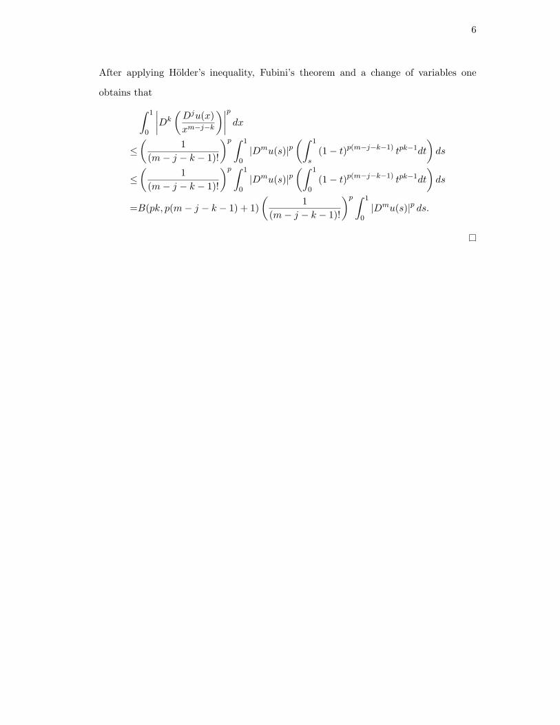


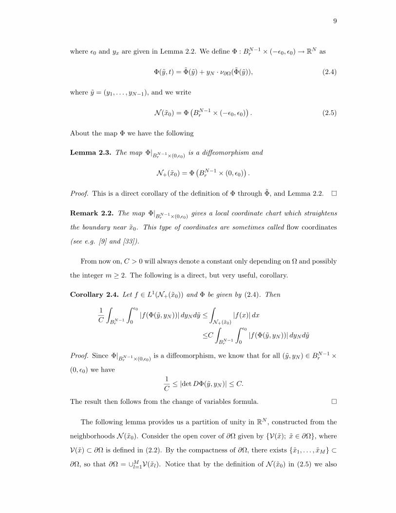


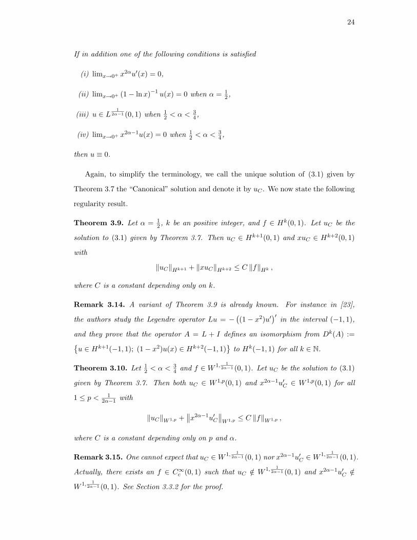


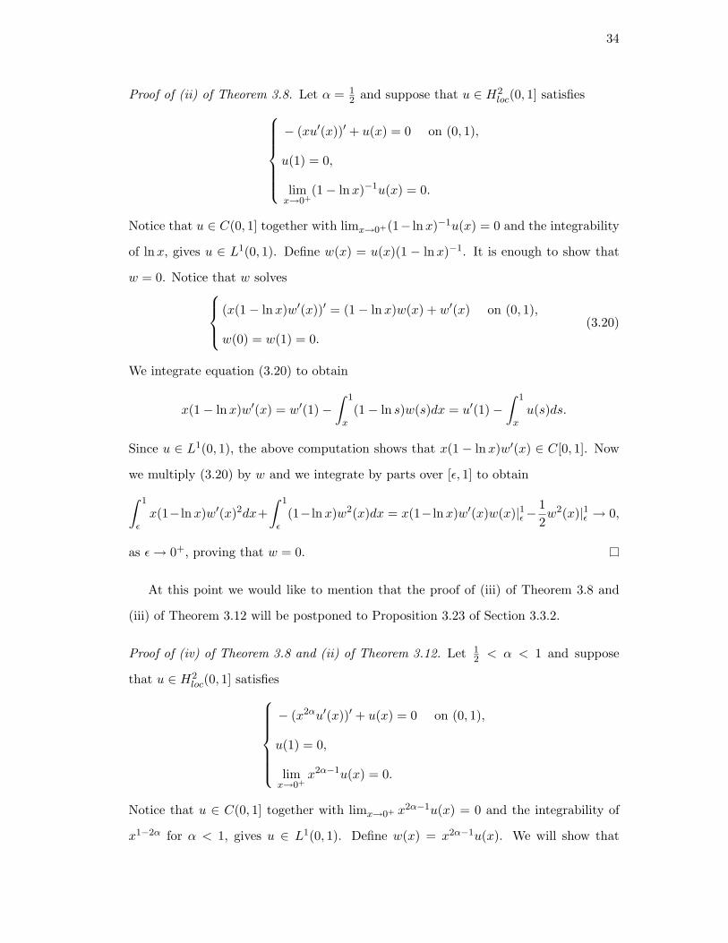


![Sturm-Liouville boundary value problems and Lagrange ... · the classical theory of Sturm-Liouville di"erential equations is developed by Titchmarsh [20], Coddington and Levinson](https://static.documents.pub/doc/80x56/5fa3e6c67d10916c566e14e7/sturm-liouville-boundary-value-problems-and-lagrange-the-classical-theory-of.jpg)


