On an Extension of Condition Number Theory to Non-Conic Convex Optimization Robert M. Freund * and Fernando Ord´ o˜ nez † February 14, 2003 Abstract The purpose of this paper is to extend, as much as possible, the modern theory of condition numbers for conic convex optimization: z * := min x c t x s.t. Ax - b ∈ C Y x ∈ C X , to the more general non-conic format: (GP d ) z * := min x c t x s.t. Ax - b ∈ C Y x ∈ P, where P is any closed convex set, not necessarily a cone, which we call the ground- set. Although any convex problem can be transformed to conic form, such trans- formations are neither unique nor natural given the natural description of many problems, thereby diminishing the relevance of data-based condition number the- ory. Herein we extend the modern theory of condition numbers to the problem format (GP d ). As a byproduct, we are able to state and prove natural extensions of many theorems from the conic-based theory of condition numbers to this broader problem format. Key words: Condition number, convex optimization, conic optimization, duality, sen- sitivity analysis, perturbation theory. * MIT Sloan School of Management, 50 Memorial Drive, Cambridge, MA 02142, USA, email: rfre- [email protected]† Industrial and Systems Engineering, University of Southern California, GER-247, Los Angeles, CA 90089-0193, USA, email: [email protected]1
Transcript
On an Extension of Condition Number Theory toNon-Conic Convex Optimization
Robert M. Freund∗ and Fernando Ordonez†
February 14, 2003
Abstract
The purpose of this paper is to extend, as much as possible, the modern theoryof condition numbers for conic convex optimization:
z∗ := minx ctxs.t. Ax− b ∈ CY
x ∈ CX ,
to the more general non-conic format:
(GPd)z∗ := minx ctx
s.t. Ax− b ∈ CY
x ∈ P ,
where P is any closed convex set, not necessarily a cone, which we call the ground-set. Although any convex problem can be transformed to conic form, such trans-formations are neither unique nor natural given the natural description of manyproblems, thereby diminishing the relevance of data-based condition number the-ory. Herein we extend the modern theory of condition numbers to the problemformat (GPd). As a byproduct, we are able to state and prove natural extensions ofmany theorems from the conic-based theory of condition numbers to this broaderproblem format.
∗MIT Sloan School of Management, 50 Memorial Drive, Cambridge, MA 02142, USA, email: [email protected]
†Industrial and Systems Engineering, University of Southern California, GER-247, Los Angeles, CA90089-0193, USA, email: [email protected]
1
1 Introduction
The modern theory of condition numbers for convex optimization problems was devel-oped by Renegar in [16] and [17] for convex optimization problems in the following conicformat:
(CPd)z∗ := minx ctx
s.t. Ax− b ∈ CY
x ∈ CX ,(1)
where CX ⊆ X and CY ⊆ Y are closed convex cones, A is a linear operator from then-dimensional vector space X to the m-dimensional vector space Y , b ∈ Y , and c ∈ X ∗
(the space of linear functionals on X ). The data d for (CPd) is defined as d := (A, b, c).
The theory of condition numbers for (CPd) focuses on three measures – ρP (d), ρD(d),and C(d), to bound various behavioral and computational quantities pertaining to(CPd). The quantity ρP (d) is called the “distance to primal infeasibility” and is thesmallest data perturbation ∆d for which (CPd+∆d) is infeasible. The quantity ρD(d) iscalled the “distance to dual infeasibility” for the conic dual (CDd) of (CPd):
(CDd)z∗ := maxy bty
s.t. c− Aty ∈ C∗X
y ∈ C∗Y ,
(2)
and is defined similarly to ρP (d) but using the conic dual problem instead (which conve-niently is of the same general conic format as the primal problem). The quantity C(d)is called the “condition measure” or the “condition number” of the problem instance dand is a (positively) scale-invariant reciprocal of the smallest data perturbation ∆d thatwill render the perturbed data instance either primal or dual infeasible:
C(d) :=‖d‖
min{ρP (d), ρD(d)}, (3)
for a suitably defined norm ‖ · ‖ on the space of data instances d. A problem is called“ill-posed” if min{ρP (d), ρD(d)} = 0, equivalently C(d) = ∞. These three conditionmeasure quantities have been shown in theory to be connected to a wide variety ofbounds on behavioral characteristics of (CPd) and its dual, including bounds on sizesof feasible solutions, bounds on sizes of optimal solutions, bounds on optimal objectivevalues, bounds on the sizes and aspect ratios of inscribed balls in the feasible region,bounds on the rate of deformation of the feasible region under perturbation, bounds onchanges in optimal objective values under perturbation, and numerical bounds relatedto the linear algebra computations of certain algorithms, see [16], [5], [4], [6], [7], [8],[21], [19], [22], [20], [14], [15]. In the context of interior-point methods for linear andsemidefinite optimization, these same three condition measures have also been shown to
2
be connected to various quantities of interest regarding the central trajectory, see [10]and [11]. The connection of these condition measures to the complexity of algorithmshas been shown in [6], [7], [17], [2], and [3], and some of the references contained therein.
The conic format (CPd) covers a very general class of convex problems; indeed anyconvex optimization problem can be transformed to an equivalent instance of (CPd).However, such transformations are not necessarily unique and are sometimes ratherunnatural given the “natural” description and the natural data for the problem. Thecondition number theory developed in the aforementioned literature pertains only toconvex optimization problems in conic form, and the relevance of this theory is dimin-ished to the extent that many practical convex optimization problems are not conveyedin conic format. Furthermore, the transformation of a problem to conic form can resultin dramatically different condition numbers depending on the choice of transformation,see the example in Section 2 of [13].
Motivated to overcome these shortcomings, herein we extend the condition numbertheory to non-conic convex optimization problems. We consider the more general formatfor convex optimization:
(GPd)z∗(d) = min ctx
s.t. Ax− b ∈ CY
x ∈ P ,(4)
where P is allowed to be any closed convex set, possibly unbounded, and possibly withoutinterior. For example, P could be the solution set of box constraints of the form l ≤ x ≤ uwhere some components of l and/or u might be unbounded, or P might be the solutionof network flow constraints of the form Nx = g, x ≥ 0. And of course, P might also be aclosed convex cone. We call P the ground-set and we refer to (GPd) as the “ground-setmodel” (GSM) format.
We present the definition of the condition number for problem instances of the moregeneral GSM format in Section 2, where we also demonstrate some basic properties. Anumber of results from condition number theory are extended to the GSM format inthe subsequent sections of the paper. In Section 3 we prove that a problem instancewith a finite condition number has primal and dual Slater points, which in turn impliesthat strong duality holds for the problem instance and its dual. In Section 4 we providecharacterizations of the condition number as the solution to associated optimizationproblems. In Section 5 we show that if the condition number of a problem instanceis finite, then there exist primal and dual interior solutions that have good geometricproperties. In Section 6 we show that the rate of deformation of primal and dual feasibleregions and optimal objective function values due to changes in the data are boundedby functions of the condition number. Section 7 contains concluding remarks.
We now present the notation and general assumptions that we will use throughoutthe paper.
3
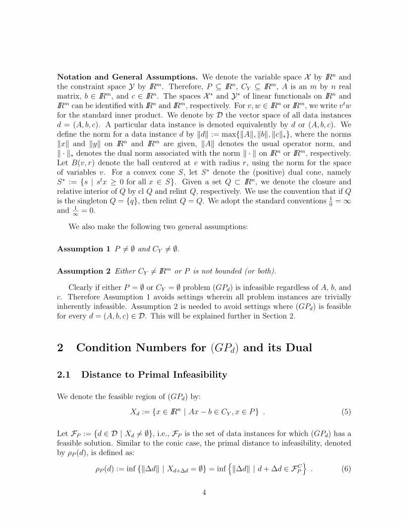
Notation and General Assumptions. We denote the variable space X by IRn andthe constraint space Y by IRm. Therefore, P ⊆ IRn, CY ⊆ IRm, A is an m by n realmatrix, b ∈ IRm, and c ∈ IRn. The spaces X ∗ and Y∗ of linear functionals on IRn andIRm can be identified with IRn and IRm, respectively. For v, w ∈ IRn or IRm, we write vtwfor the standard inner product. We denote by D the vector space of all data instancesd = (A, b, c). A particular data instance is denoted equivalently by d or (A, b, c). Wedefine the norm for a data instance d by ‖d‖ := max{‖A‖, ‖b‖, ‖c‖∗}, where the norms‖x‖ and ‖y‖ on IRn and IRm are given, ‖A‖ denotes the usual operator norm, and‖ · ‖∗ denotes the dual norm associated with the norm ‖ · ‖ on IRn or IRm, respectively.Let B(v, r) denote the ball centered at v with radius r, using the norm for the spaceof variables v. For a convex cone S, let S∗ denote the (positive) dual cone, namelyS∗ := {s | stx ≥ 0 for all x ∈ S}. Given a set Q ⊂ IRn, we denote the closure andrelative interior of Q by cl Q and relint Q, respectively. We use the convention that if Qis the singleton Q = {q}, then relint Q = Q. We adopt the standard conventions 1
0= ∞
and 1∞ = 0.
We also make the following two general assumptions:
Assumption 1 P 6= ∅ and CY 6= ∅.
Assumption 2 Either CY 6= IRm or P is not bounded (or both).
Clearly if either P = ∅ or CY = ∅ problem (GPd) is infeasible regardless of A, b, andc. Therefore Assumption 1 avoids settings wherein all problem instances are triviallyinherently infeasible. Assumption 2 is needed to avoid settings where (GPd) is feasiblefor every d = (A, b, c) ∈ D. This will be explained further in Section 2.
2 Condition Numbers for (GPd) and its Dual
2.1 Distance to Primal Infeasibility
We denote the feasible region of (GPd) by:
Xd := {x ∈ IRn | Ax− b ∈ CY , x ∈ P} . (5)
Let FP := {d ∈ D | Xd 6= ∅}, i.e., FP is the set of data instances for which (GPd) has afeasible solution. Similar to the conic case, the primal distance to infeasibility, denotedby ρP (d), is defined as:
ρP (d) := inf {‖∆d‖ | Xd+∆d = ∅} = inf{‖∆d‖ | d + ∆d ∈ FC
P
}. (6)
4
2.2 The Dual Problem and Distance to Dual Infeasibility
In the case when P is a cone, the conic dual problem (2) is of the same basic format asthe primal problem. However, when P is not a cone, we must first develop a suitabledual problem, which we do in this subsection. Before doing so we introduce a dualpair of cones associated with the ground-set P . Define the closed convex cone C byhomogenizing P to one higher dimension:
C := cl {(x, t) ∈ IRn × IR | x ∈ tP, t > 0} , (7)
and note that C = {(x, t) ∈ IRn × IR | x ∈ tP, t > 0} ∪ (R× {0}) where R is the reces-sion cone of P , namely
R := {v ∈ IRn | there exists x ∈ P for which x + θv ∈ P for all θ ≥ 0} . (8)
It is straightforward to show that the (positive) dual cone C∗ of C is
C∗ := {(s, u) ∈ IRn × IR | stx + u · t ≥ 0 for all (x, t) ∈ C}= {(s, u) ∈ IRn × IR | stx + u ≥ 0, for all x ∈ P}= {(s, u) ∈ IRn × IR | infx∈P stx + u ≥ 0} .
(9)
The standard Lagrangian dual of (GPd) can be constructed as:
maxy∈C∗
Y
infx∈P
{ctx + (b− Ax)ty}
which we re-write as:maxy∈C∗
Y
infx∈P
{bty + (c− Aty)tx} . (10)
With the help of (9) we re-write (10) as:
(GDd)z∗(d) = maxy,u bty − u
s.t. (c− Aty, u) ∈ C∗
y ∈ C∗Y .
(11)
We consider the formulation (11) to be the dual problem of (4). The feasible region of(GDd) is:
Yd := {(y, u) ∈ IRm × IR | (c− Aty, u) ∈ C∗, y ∈ C∗Y }. (12)
Let FD := {d ∈ D | Yd 6= ∅}, i.e., FD is the set of data instances for which (GDd) has afeasible solution. The dual distance to infeasibility, denoted by ρD(d), is defined as:
ρD(d) := inf {‖∆d‖ | Yd+∆d = ∅} = inf{‖∆d‖ | d + ∆d ∈ FC
D
}. (13)
5
We also present an alternate form of (11), which does not use the auxiliary variableu, based on the function u(·) defined by
u(s) := − infx∈P
stx . (14)
It follows from Theorem 5.5 in [18] that u(·), the support function of the set P , is aconvex function. The epigraph of u(·) is:
epi u(·) := {(s, v) ∈ IRn × IR | v ≥ u(s)} ,
and the projection of the epigraph onto the space of the variables s is the effectivedomain of u(·):
Evaluating the inclusion (y, u) ∈ Yd is not necessarily an easy task, as it involveschecking the inclusion (c − Aty, u) ∈ C∗, and C∗ is an implicitly defined cone. A veryuseful tool for evaluating the inclusion (y, u) ∈ Yd is given in the following proposition,where recall from (8) that R is the recession cone of P .
Proposition 1 If y satisfies y ∈ C∗Y and c − Aty ∈ relintR∗, then u(c − Aty) is finite,
and for all u ≥ u(c− Aty) it holds that (y, u) is feasible for (GDd).
Proof: Note from Proposition 11 of the Appendix that cl effdom u(·) = R∗ andfrom Proposition 12 of the Appendix that c − Aty ∈ relintR∗ = relint cl effdom u(·) =relint effdom u(·) ⊆ effdom u(·). This shows that u(c−Aty) is finite and (c−Aty, u(c−Aty)) ∈ C∗. Therefore (y, u) is feasible for (GDd) for all u ≥ u(c− Aty).
2.3 Condition Number
A data instance d = (A, b, c) is consistent if both the primal and dual problems havefeasible solutions. Let F denote the set of consistent data instances, namely F :=
6
FP ∩ FD = {d ∈ D | Xd 6= ∅ and Yd 6= ∅}. For d ∈ F , the distance to infeasibility isdefined as:
ρ(d) := min {ρP (d), ρD(d)}= inf {‖∆d‖ | Xd+∆d = ∅ or Yd+∆d = ∅} ,
(16)
the interpretation being that ρ(d) is the size of the smallest perturbation of d which willrender the perturbed problem instance either primal or dual infeasible. The conditionnumber of the instance d is defined as
C(d) :=
‖d‖ρ(d)
ρ(d) > 0
∞ ρ(d) = 0 ,
which is a (positive) scale-invariant reciprocal of the distance to infeasibility. This def-inition of condition number for convex optimization problems was first introduced byRenegar for problems in conic form in [16] and [17].
2.4 Basic Properties of ρP (d), ρD(d), and C(d), and AlternativeDuality Results
The need for Assumptions 1 and 2 is demonstrated by the following:
Proposition 2 For any data instance d ∈ D,
1. ρP (d) = ∞ if and only if CY = IRm.
2. ρD(d) = ∞ if and only if P is bounded.
The proof of this proposition relies on Lemmas 1 and 2, which are versions of “theo-rems of the alternative” for primal and dual feasibility of (GPd) and (GDd). These twolemmas are stated and proved at the end of this section.
Proof of Proposition 2: Clearly CY = IRm implies that ρP (d) = ∞. Also, if P isbounded, then R = {0} and R∗ = IRn, whereby from Proposition 1 we have that (GDd)is feasible for any d, and so ρD(d) = ∞. Therefore for both items it only remains toprove the converse implication. Recall that we denote d = (A, b, c).
Assume that ρP (d) = ∞, and suppose that CY 6= IRm. Then C∗Y 6= {0}, and consider
a point y ∈ C∗Y , y 6= 0. Define the perturbation ∆d = (∆A, ∆b, ∆c) = (−A,−b + y,−c)
and d = d + ∆d. Then the point (y, u) =(y, yty
2
)satisfies the alternative system (A2d)
of Lemma 1 for the data d = (0, y, 0), whereby Xd = ∅. Therefore ‖d−d‖ ≥ ρP (d) = ∞,a contradiction, and so CY = IRm.
7
Now assume that ρD(d) = ∞, and suppose that P is not bounded, and so R 6= {0}.Consider x ∈ R, x 6= 0, and define the perturbation ∆d = (−A,−b,−c − x). Then thepoint x satisfies the alternative system (B2d) of Lemma 2 for the data d = d + ∆d =(0, 0,−x), whereby Yd = ∅. Therefore ‖d− d‖ ≥ ρD(d) = ∞, a contradiction, and so Pis bounded.
Remark 1 If d ∈ F , then C(d) ≥ 1.
Proof: Consider the data instance d0 = (0, 0, 0). Note that Xd0 = P 6= ∅ andYd0 = C∗
Y × IR+ 6= ∅, therefore d0 ∈ F . If CY 6= IRm, consider b ∈ IRm \ CY , b 6= 0, andfor any ε > 0 define the instance dε = (0,−εb, 0). This instance is such that for anyε > 0, Xdε = ∅, which means that dε ∈ FC
P and therefore ρP (d) ≤ infε>0 ‖d− dε‖ ≤ ‖d‖.If CY = IRm, then Assumption 2 implies that P is unbounded. This means that thereexists a ray r ∈ R, r 6= 0. For any ε > 0 the instance dε = (0, 0,−εr) is such thatYdε = ∅, which means that dε ∈ FC
D and therefore ρD(d) ≤ infε>0 ‖d− dε‖ ≤ ‖d‖ .
In each case we have ρ(d) = min{ρP (d), ρP (d)} ≤ ‖d‖, which implies the result.
The following two lemmas present weak and strong alternative results for (GPd) and(GDd), and are used in the proofs of Proposition 2 and elsewhere.
Lemma 1 Consider the following systems with data d = (A, b, c):
(Xd)Ax− b ∈ CY
x ∈ P, (A1d)
(−Aty, u) ∈ C∗
bty ≥ uy 6= 0y ∈ C∗
Y
, (A2d)(−Aty, u) ∈ C∗
bty > uy ∈ C∗
Y
If system (Xd) is infeasible, then system (A1d) is feasible. Conversely, if system(A2d) is feasible, then system (Xd) is infeasible.
Proof: Assume that system (Xd) is infeasible. This implies that
b 6∈ S := {Ax− v | x ∈ P, v ∈ CY } ,
which is a nonempty convex set. Using Proposition 10 we can separate b from S andtherefore there exists y 6= 0 such that
yt(Ax− v) ≤ ytb for all x ∈ P, v ∈ CY .
Set u := ytb, then the inequality implies that y ∈ C∗Y and that (−Aty)tx+u ≥ 0 for any
x ∈ P . Therefore (−Aty, u) ∈ C∗ and (y, u) satisfies system (A1d).
Conversely, if both (A2d) and (Xd) are feasible then
0 ≤ yt(Ax− b) = (Aty)tx− bty < −((−Aty)tx + u
)≤ 0 .
8
Lemma 2 Consider the following systems with data d = (A, b, c):
(Yd)(c− Aty, u) ∈ C∗
y ∈ C∗Y
, (B1d)
Ax ∈ CY
ctx ≤ 0x 6= 0x ∈ R
, (B2d)Ax ∈ CY
ctx < 0x ∈ R
If system (Yd) is infeasible, then system (B1d) is feasible. Conversely, if system (B2d)is feasible, then system (Yd) is infeasible.
Proof: Assume that system (Yd) is infeasible, this implies that
(0, 0, 0) 6∈ S :={(s, v, q) | ∃ y, u s.t. (c− Aty, u) + (s, v) ∈ C∗, y + q ∈ C∗
Y
},
which is a nonempty convex set. Using Proposition 10 we separate the point (0, 0, 0) fromS and therefore there exists (x, δ, z) 6= 0 such that xts+ δv + ztq ≥ 0 for all (s, v, q) ∈ S.For any (y, u), (s, v) ∈ C∗, and q ∈ C∗
Y , define s = −(c − Aty) + s, v = −u + v, andq = −y + q. By construction (s, v, q) ∈ S and therefore for any y, u, (s, v) ∈ C∗, q ∈ C∗
Y
we have−xtc + (Ax− z)t y + xts− δu + δv + ztq ≥ 0 .
The above inequality implies that δ = 0, Ax = z ∈ CY , x ∈ R, and ctx ≤ 0. In additionx 6= 0, because otherwise (x, δ, z) = (x, 0, Ax) = 0. Therefore (B1d) is feasible.
Conversely, if both (B2d) and (Yd) are feasible then
0 ≤ xt(c− Aty) = ctx− ytAx < −ytAx ≤ 0 .
3 Slater Points, Distance to Infeasibility, and Strong
Duality
In this section we prove that the existence of a Slater point in either (GPd) or (GDd) issufficient to guarantee that strong duality holds for these problems. We then show thata positive distance to infeasibility implies the existence of Slater points, and use theseresults to show that strong duality holds whenever ρP (d) > 0 or ρD(d) > 0. We firststate a weak duality result.
Proposition 3 Weak duality holds between (GPd) and (GDd), that is, z∗(d) ≤ z∗(d) .
Proof: Consider x and (y, u) feasible for (GPd) and (GDd), respectively. Then
0 ≤(c− Aty
)tx + u = ctx− ytAx + u ≤ ctx− bty + u,
9
where the last inequality follows from yt(Ax− b) ≥ 0. Therefore z∗(d) ≥ z∗(d).
A classic constraint qualification in the history of constrained optimization is theexistence of a Slater point in the feasible region, see for example Theorem 30.4 of [18]or Chapter 5 of [1]. We now define a Slater point for problems in the GSM format.
Definition 1 A point x is a Slater point for problem (GPd) if
x ∈ relintP and Ax− b ∈ relintCY .
A point (y, u) is a Slater point for problem (GDd) if
y ∈ relintC∗Y and (c− Aty, u) ∈ relintC∗ .
We now present the statements of the main results of this section, deferring theproofs to the end of the section. The following two theorems show that the existence ofa Slater point in the primal or dual is sufficient to guarantee strong duality as well asattainment in the dual or the primal problem, respectively.
Theorem 1 If x′ is a Slater point for problem (GPd), then z∗(d) = z∗(d). If in additionz∗(d) > −∞, then Yd 6= ∅ and problem (GDd) attains its optimum.
Theorem 2 If (y′, u′) is a Slater point for problem (GDd), then z∗(d) = z∗(d). If inaddition z∗(d) < ∞, then Xd 6= ∅ and problem (GPd) attains its optimum.
The next three results show that a positive distance to infeasibility is sufficient toguarantee the existence of Slater point for the primal and the dual problems, respectively,and hence is sufficient to ensure that strong duality holds. The fact that a positivedistance to infeasibility implies the existence of an interior point in the feasible regionis shown for the conic case in Theorems 15, 17, and 19 in [8] and Theorem 3.1 in [17].
Theorem 3 Suppose that ρP (d) > 0. Then there exists a Slater point for (GPd).
Theorem 4 Suppose that ρD(d) > 0. Then there exists a Slater point for (GDd).
Corollary 1 (Strong Duality) If ρP (d) > 0 or ρD(d) > 0, then z∗(d) = z∗(d). Ifρ(d) > 0, then both the primal and the dual attain their respective optimal values.
Proof: The proof of this result is a straightforward consequence of Theorems 1, 2,3, and 4.
10
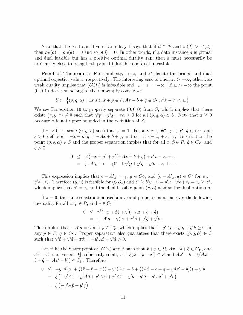
Note that the contrapositive of Corollary 1 says that if d ∈ F and z∗(d) > z∗(d),then ρP (d) = ρD(d) = 0 and so ρ(d) = 0. In other words, if a data instance d is primaland dual feasible but has a positive optimal duality gap, then d must necessarily bearbitrarily close to being both primal infeasible and dual infeasible.
Proof of Theorem 1: For simplicity, let z∗ and z∗ denote the primal and dualoptimal objective values, respectively. The interesting case is when z∗ > −∞, otherwiseweak duality implies that (GDd) is infeasible and z∗ = z∗ = −∞. If z∗ > −∞ the point(0, 0, 0) does not belong to the non-empty convex set
S :={(p, q, α) | ∃x s.t. x + p ∈ P, Ax− b + q ∈ CY , ctx− α < z∗
}.
We use Proposition 10 to properly separate (0, 0, 0) from S, which implies that thereexists (γ, y, π) 6= 0 such that γtp + ytq + πα ≥ 0 for all (p, q, α) ∈ S. Note that π ≥ 0because α is not upper bounded in the definition of S.
If π > 0, re-scale (γ, y, π) such that π = 1. For any x ∈ IRn, p ∈ P , q ∈ CY , andε > 0 define p = −x + p, q = −Ax + b + q, and α = ctx − z∗ + ε. By construction thepoint (p, q, α) ∈ S and the proper separation implies that for all x, p ∈ P , q ∈ CY , andε > 0
0 ≤ γt(−x + p) + yt(−Ax + b + q) + ctx− z∗ + ε
= (−Aty + c− γ)tx + γtp + ytq + ytb− z∗ + ε .
This expression implies that c − Aty = γ, y ∈ C∗Y , and (c − Aty, u) ∈ C∗ for u :=
ytb−z∗. Therefore (y, u) is feasible for (GDd) and z∗ ≥ bty−u = bty−ytb+z∗ = z∗ ≥ z∗,which implies that z∗ = z∗ and the dual feasible point (y, u) attains the dual optimum.
If π = 0, the same construction used above and proper separation gives the followinginequality for all x, p ∈ P , and q ∈ CY
0 ≤ γt(−x + p) + yt(−Ax + b + q)
= (−Aty − γ)tx + γtp + ytq + ytb .
This implies that −Aty = γ and y ∈ C∗Y , which implies that −ytAp + ytq + ytb ≥ 0 for
any p ∈ P , q ∈ CY . Proper separation also guarantees that there exists (p, q, α) ∈ Ssuch that γtp + ytq + πα = −ytAp + ytq > 0.
Let x′ be the Slater point of (GPd) and x such that x + p ∈ P , Ax− b + q ∈ CY , andctx− α < z∗ For all |ξ| sufficiently small, x′ + ξ(x + p− x′) ∈ P and Ax′ − b + ξ(Ax−b + q − (Ax′ − b)) ∈ CY . Therefore
a contradiction, since ξ can be negative and −ytAp + ytq > 0. Therefore π 6= 0,completing the proof.
Proof of Theorem 2: For simplicity, let z∗ and z∗ denote the primal and dualoptimal objective values respectively. The interesting case is when z∗ < ∞, otherwiseweak duality implies that (GPd) is infeasible and z∗ = z∗ = ∞. If z∗ < ∞ the point(0, 0, 0, 0) does not belong to the non-empty convex set
S :={(s, v, q, α) | ∃y, u s.t. (c− Aty, u) + (s, v) ∈ C∗, y + q ∈ C∗
Y , bty − u + α > z∗}
.
We use Proposition 10 to properly separate (0, 0, 0, 0) from S, which implies that thereexists (x, β, γ, δ) 6= 0 such that xts + βv + γtq + δα ≥ 0 for all (s, v, q, α) ∈ S. Note thatδ ≥ 0 because α is not upper bounded in the definition of S.
If δ > 0, re-scale (x, β, γ, δ) such that δ = 1. For any y ∈ IRm, u ∈ IR, (s, v) ∈ C∗,q ∈ C∗
Y , and ε > 0, define s = −c+Aty+s, v = −u+v, q = −y+q, and α = z∗−bty+u+ε.By construction the point (s, v, q, α) ∈ S and proper separation implies that for all y, u,(s, v) ∈ C∗, q ∈ C∗
This implies that Ax− b = γ ∈ CY , β = 1, ctx ≤ z∗, and (x, 1) ∈ C, which means thatx ∈ P . Therefore x is feasible for (GPd) and z∗ ≥ ctx ≥ z∗ ≥ z∗, which implies thatz∗ = z∗ and the primal feasible point x attains the optimum.
If δ = 0, the same construction used above and proper separation gives the followinginequality for all y, u, (s, v) ∈ C∗, q ∈ C∗
Y
0 ≤ xt(−c + Aty + s) + β(−u + v) + γt(−y + q)
= (Ax− γ)t y + (x, β)t(s, v)− βu + γtq − ctx .
This implies that Ax = γ ∈ CY , β = 0, which means that xts + xtAtq − ctx ≥ 0 forany (s, u) ∈ C∗ and q ∈ C∗
Y . The proper separation also guarantees that there exists(s, v, q, α) ∈ S such that xts + βv + γtq = xts + xtAtq > 0.
Let (y′, u′) be the Slater point of (GDd) and (y, u) such that (c−Aty+ s, u+ v) ∈ C∗,y + q ∈ C∗
Y , and bty − u + α > z∗. Then for all |ξ| sufficiently small, we have thaty′ + ξ (y + q − y′) ∈ C∗
a contradiction, since ξ can be negative and xts+xtAtq > 0. Therefore δ 6= 0, completingthe proof.
Proof of Theorem 3: Equation (6) and ρP (d) > 0 imply that Xd 6= ∅. Assume that Xd
contains no Slater point, then relintCY ∩{Ax− b | x ∈ relintP} = ∅ and these nonemptyconvex sets can be separated using Proposition 10. Therefore there exists y 6= 0 suchthat for any s ∈ CY , x ∈ P we have
yts ≥ yt (Ax− b) .
Let u = ytb; from the inequality above we have that y ∈ C∗Y and −ytAx + u ≥ 0 for
any x ∈ P , which implies that (−Aty, u) ∈ C∗. Define bε = b + ε‖y‖∗ y, with y given by
Proposition 9 such that ‖y‖ = 1 and yty = ‖y‖∗. Then the point (y, u) is feasible forProblem (A2dε) of Lemma 1 with data dε = (A, bε, c) for any ε > 0. This implies thatXdε = ∅ and therefore ρP (d) ≤ infε>0 ‖d− dε‖ = infε>0
ε‖y‖∗ = 0, a contradiction.
Proof of Theorem 4: Equation (13) and ρD(d) > 0 imply that Yd 6= ∅. Assume thatYd contains no Slater point. Consider the nonempty convex set S defined by:
S :={(
c− Aty, u)| y ∈ relintC∗
Y , u ∈ IR}
.
No Slater point in the dual implies that relintC∗ ∩ S = ∅. Therefore we can properlyseparate these two nonempty convex sets using Proposition 10, whereby there exists(x, t) 6= 0 such that for any (s, v) ∈ C∗, y ∈ C∗
Y , u ∈ IR we have
xts + tv ≥ xt(c− Aty
)+ tu .
The above inequality implies that Ax ∈ CY , ctx ≤ 0, (x, t) ∈ C, and t = 0. This lastfact implies that x 6= 0 and x ∈ R. Let x be such that ‖x‖∗ = 1 and xtx = ‖x‖ (seeProposition 9). For any ε > 0, define cε = c − ε
‖x‖ x. Then the point x is feasible for
Problem (B2dε) of Lemma 2 with data dε = (A, b, cε). This implies then that Ydε = ∅and consequently ρD(d) ≤ infε>0 ‖d− dε‖ = infε>0
ε‖x‖ = 0, a contradiction.
The contrapositives of Theorems 3 and 4 are not true. Consider for example the data
A =
[0 00 0
], b =
(−10
), and c =
(10
),
and the sets CY = IR+ × {0} and P = CX = IR+ × IR. Problem (GPd) for this examplehas a Slater point at (1, 0), and ρP (d) = 0 (perturbing by ∆b = (0, ε) makes the probleminfeasible for any ε.) Problem (GDd) for the same example has a Slater point at (1, 0)and ρD(d) = 0 (perturbing by ∆c = (0, ε) makes the problem infeasible for any ε).
13
4 Characterization of ρP (d) and ρD(d) via Associated
Optimization Problems
Equation (16) shows that to characterize ρ(d) for consistent data instances d ∈ F , itis sufficient to express ρP (d) and ρD(d) in a convenient form. Below we show thatthese distances to infeasibility can be obtained as the solutions of certain associatedoptimization problems. These results can be viewed as an extension to problems not inconic form of Theorem 3.5 of [17], and Theorems 1 and 2 of [8].
Theorem 5 Suppose that Xd 6= ∅. Then ρP (d) = jP (d) = rP (d), where
jP (d) = min max {‖Aty + s‖∗, |bty − u|}‖y‖∗ = 1y ∈ C∗
Y
(s, u) ∈ C∗
(17)
and
rP (d) = min max θ‖v‖ ≤ 1 Ax− bt− vθ ∈ CY
v ∈ IRm ‖x‖+ |t| ≤ 1(x, t) ∈ C .
(18)
Theorem 6 Suppose that Yd 6= ∅. Then ρD(d) = jD(d) = rD(d), where
jD(d) = min max {‖Ax− p‖, |ctx + g|}‖x‖ = 1x ∈ Rp ∈ CY
g ≥ 0
(19)
and
rD(d) = min max θ‖v‖∗ ≤ 1 −Aty + cδ − θv ∈ R∗
v ∈ IRn ‖y‖∗ + |δ| ≤ 1y ∈ C∗
Y
δ ≥ 0 .
(20)
Proof of Theorem 5: Assume that jP (d) > ρP (d), then there exists a data instanced = (A, b, c) that is primal infeasible and ‖A − A‖ < jP (d), ‖b − b‖ < jP (d), and
14
‖c− c‖∗ < jP (d). From Lemma 1 there is a point (y, u) that satisfies the following:
(−Aty, u) ∈ C∗
bty ≥ uy 6= 0y ∈ C∗
Y .
Scale y such that ‖y‖∗ = 1, then (y, s, u) = (y,−Aty, bty) is feasible for (17) and
‖Aty + s‖∗ = ‖Aty − Aty‖∗ ≤ ‖A− A‖‖y‖∗ < jP (d)
|bty − u| = |bty − bty| ≤ ‖b− b‖‖y‖∗ < jP (d).
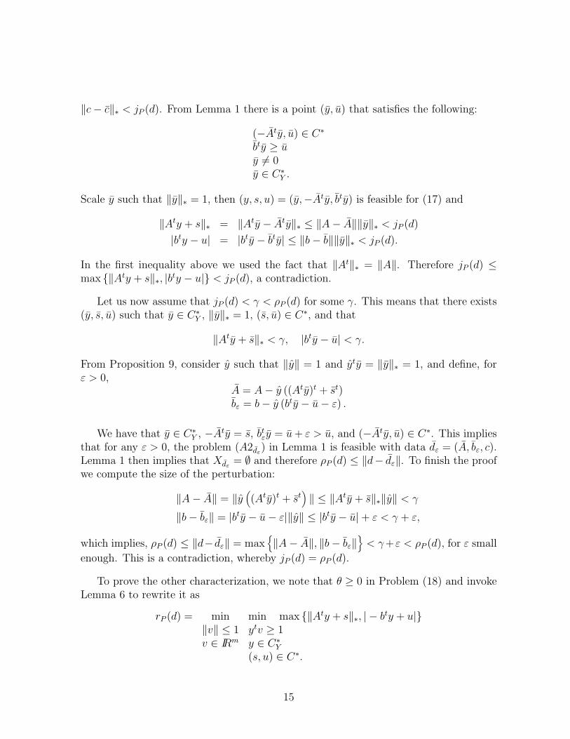
In the first inequality above we used the fact that ‖At‖∗ = ‖A‖. Therefore jP (d) ≤max {‖Aty + s‖∗, |bty − u|} < jP (d), a contradiction.
Let us now assume that jP (d) < γ < ρP (d) for some γ. This means that there exists(y, s, u) such that y ∈ C∗
Y , ‖y‖∗ = 1, (s, u) ∈ C∗, and that
‖Aty + s‖∗ < γ, |bty − u| < γ.
From Proposition 9, consider y such that ‖y‖ = 1 and yty = ‖y‖∗ = 1, and define, forε > 0,
A = A− y ((Aty)t + st)bε = b− y (bty − u− ε) .
We have that y ∈ C∗Y , −Aty = s, bt
εy = u + ε > u, and (−Aty, u) ∈ C∗. This impliesthat for any ε > 0, the problem (A2dε
) in Lemma 1 is feasible with data dε = (A, bε, c).Lemma 1 then implies that Xdε
= ∅ and therefore ρP (d) ≤ ‖d− dε‖. To finish the proofwe compute the size of the perturbation:
enough. This is a contradiction, whereby jP (d) = ρP (d).
To prove the other characterization, we note that θ ≥ 0 in Problem (18) and invokeLemma 6 to rewrite it as
rP (d) = min min max {‖Aty + s‖∗, | − bty + u|}‖v‖ ≤ 1 ytv ≥ 1v ∈ IRm y ∈ C∗
Y
(s, u) ∈ C∗.
15
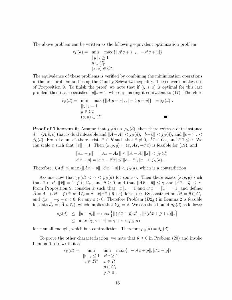
The above problem can be written as the following equivalent optimization problem:
rP (d) = min max {‖Aty + s‖∗, | − bty + u|}‖y‖∗ ≥ 1y ∈ C∗
Y
(s, u) ∈ C∗.
The equivalence of these problems is verified by combining the minimization operationsin the first problem and using the Cauchy-Schwartz inequality. The converse makes useof Proposition 9. To finish the proof, we note that if (y, s, u) is optimal for this lastproblem then it also satisfies ‖y‖∗ = 1, whereby making it equivalent to (17). Therefore
rP (d) = min max {‖Aty + s‖∗, | − bty + u|} = jP (d) .‖y‖∗ = 1y ∈ C∗
Y
(s, u) ∈ C∗
Proof of Theorem 6: Assume that jD(d) > ρD(d), then there exists a data instanced = (A, b, c) that is dual infeasible and ‖A− A‖ < jD(d), ‖b− b‖ < jD(d), and ‖c− c‖∗ <jD(d). From Lemma 2 there exists x ∈ R such that x 6= 0, Ax ∈ CY , and ctx ≤ 0. Wecan scale x such that ‖x‖ = 1. Then (x, p, g) = (x, Ax,−ctx) is feasible for (19), and
‖Ax− p‖ = ‖Ax− Ax‖ ≤ ‖A− A‖‖x‖ < jD(d)
|ctx + g| = |ctx− ctx| ≤ ‖c− c‖∗‖x‖ < jD(d) .
Therefore, jD(d) ≤ max {‖Ax− p‖, |ctx + g|} < jD(d), which is a contradiction.
Assume now that jD(d) < γ < ρD(d) for some γ. Then there exists (x, p, g) suchthat x ∈ R, ‖x‖ = 1, p ∈ CY , and g ≥ 0, and that ‖Ax − p‖ ≤ γ and |ctx + g| ≤ γ.From Proposition 9, consider x such that ‖x‖∗ = 1 and xtx = ‖x‖ = 1, and define:A = A−(Ax− p) xt and cε = c− x(ctx+ g+ε), for ε > 0. By construction Ax = p ∈ CY
and ctεx = −g − ε < 0, for any ε > 0. Therefore Problem (B2dε
) in Lemma 2 is feasiblefor data dε = (A, b, cε), which implies that Ydε
for ε small enough, which is a contradiction. Therefore ρD(d) = jD(d).
To prove the other characterization, we note that θ ≥ 0 in Problem (20) and invokeLemma 6 to rewrite it as
rD(d) = min min max {‖ − Ax + p‖, |ctx + g|}‖v‖∗ ≤ 1 xtv ≥ 1v ∈ IRn x ∈ R
p ∈ CY
g ≥ 0 .
16
The above problem can be written as the following equivalent optimization problem:
rD(d) = min max {‖ − Ax + p‖, |ctx + g|}‖x‖ ≥ 1x ∈ Rp ∈ CY
g ≥ 0 .
The equivalence of these problems is verified by combining the minimization operationsin the first problem and using the Cauchy-Schwartz inequality. The converse makes useof Proposition 9. To finish the proof, we note that if (x, p, g) is optimal for this lastproblem then it also satisfies ‖x‖ = 1, whereby making it equivalent to (19). Therefore
rD(d) = min max {‖ − Ax + p‖, |ctx + g|} = jD(d) .‖x‖ = 1x ∈ Rp ∈ CY
g ≥ 0
5 Geometric Properties of the Primal and Dual Fea-
sible Regions
In Section 3 we showed that a positive primal and/or dual distance to infeasibility impliesthe existence of a primal and/or dual Slater point, respectively. We now show that apositive distance to infeasibility also implies that the corresponding feasible region has areliable solution. We consider a solution in the relative interior of the feasible region tobe a reliable solution if it has good geometric properties: it is not too far from a givenreference point, its distance to the relative boundary of the feasible region is not toosmall, and the ratio of these two quantities is not too large, where these quantities arebounded by appropriate condition numbers.
5.1 Distance to Relative Boundary, Minimum Width of Cone
An affine set T is the translation of a vector subspace L, i.e., T = a + L for some a.The minimal affine set that contains a given set S is known as the affine hull of S. Wedenote the affine hull of S by LS; it is characterized as:
LS =
{∑i∈I
αixi | αi ∈ IR, xi ∈ S,∑i∈I
αi = 1, I a finite set
},
17
see Section 1 in [18]. We denote by LS the vector subspace obtained when the affinehull LS is translated to contain the origin; i.e. for any x ∈ S, LS = LS − x. Note thatif 0 ∈ S then LS is a subspace.
Many results in this section involve the distance of a point x ∈ S to the relativeboundary of the set S, denoted by dist(x, rel∂S), defined as follows:
Definition 2 Given a non-empty set S and a point x ∈ S, the distance from x to therelative boundary of S is
dist(x, rel∂S) := inf x ‖x− x‖s.t. x ∈ LS \ S .
(21)
Note that if S is an affine set (and in particular if S is the singleton S = {s}), thendist(x, rel∂S) = ∞ for each x ∈ S.
We use the following definition of the min-width of a convex cone:
Definition 3 For a convex cone K, the min-width of K is defined by
τK := sup
{dist(y, rel∂K)
‖y‖| y ∈ K, y 6= 0
},
for K 6= {0}, and τK := ∞ if K = {0}.
The measure τK maximizes the ratio of the radius of a ball contained in the relativeinterior of K and the norm of its center, and so it intuitively corresponds to half of thevertex angle of the widest cylindrical cone contained in K. The quantity τK was calledthe “inner measure” of K for Euclidean norms in Goffin [9], and has been used morerecently for general norms in analyzing condition measures for conic convex optimization,see [6]. Note that if K is not a subspace, then τK ∈ (0, 1], and τK is attained for somey0 ∈ relintK satisfying ‖y0‖ = 1, as well as along the ray αy0 for all α > 0; and τK takeson larger values to the extent that K has larger minimum width. If K is a subspace,then τK = ∞.
5.2 Geometric Properties of the Feasible Region of GPd
In this subsection we present results concerning geometric properties of the feasibleregion Xd of (GPd). We defer all proofs to the end of the subsection.
The following proposition is an extension of Lemma 3.2 of [16] to the ground-setmodel format.
18
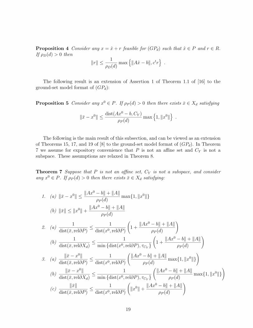
Proposition 4 Consider any x = x + r feasible for (GPd) such that x ∈ P and r ∈ R.If ρD(d) > 0 then
‖r‖ ≤ 1
ρD(d)max
{‖Ax− b‖, ctr
}.
The following result is an extension of Assertion 1 of Theorem 1.1 of [16] to theground-set model format of (GPd):
Proposition 5 Consider any x0 ∈ P . If ρP (d) > 0 then there exists x ∈ Xd satisfying
‖x− x0‖ ≤ dist(Ax0 − b, CY )
ρP (d)max
{1, ‖x0‖
}.
The following is the main result of this subsection, and can be viewed as an extensionof Theorems 15, 17, and 19 of [8] to the ground-set model format of (GPd). In Theorem7 we assume for expository convenience that P is not an affine set and CY is not asubspace. These assumptions are relaxed in Theorem 8.
Theorem 7 Suppose that P is not an affine set, CY is not a subspace, and considerany x0 ∈ P . If ρP (d) > 0 then there exists x ∈ Xd satisfying:
1. (a) ‖x− x0‖ ≤ ‖Ax0 − b‖+ ‖A‖ρP (d)
max{1, ‖x0‖}
(b) ‖x‖ ≤ ‖x0‖+‖Ax0 − b‖+ ‖A‖
ρP (d)
2. (a)1
dist(x, rel∂P )≤ 1
dist(x0, rel∂P )
(1 +
‖Ax0 − b‖+ ‖A‖ρP (d)
)
(b)1
dist(x, rel∂Xd)≤ 1
min {dist(x0, rel∂P ), τCY}
(1 +
‖Ax0 − b‖+ ‖A‖ρP (d)
)
3. (a)‖x− x0‖
dist(x, rel∂P )≤ 1
dist(x0, rel∂P )
(‖Ax0 − b‖+ ‖A‖
ρP (d)max{1, ‖x0‖}
)
(b)‖x− x0‖
dist(x, rel∂Xd)≤ 1
min {dist(x0, rel∂P ), τCY}
(‖Ax0 − b‖+ ‖A‖
ρP (d)max{1, ‖x0‖}
)
(c)‖x‖
dist(x, rel∂P )≤ 1
dist(x0, rel∂P )
(‖x0‖+
‖Ax0 − b‖+ ‖A‖ρP (d)
)
19
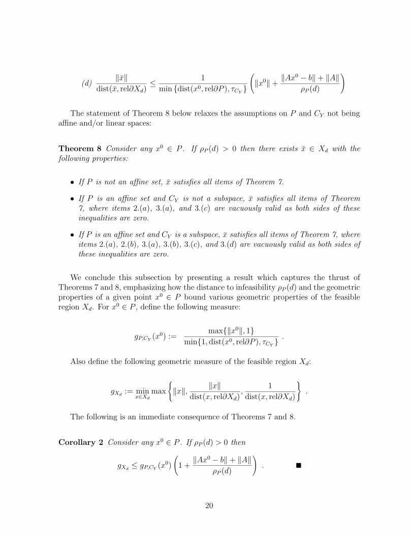
(d)‖x‖
dist(x, rel∂Xd)≤ 1
min {dist(x0, rel∂P ), τCY}
(‖x0‖+
‖Ax0 − b‖+ ‖A‖ρP (d)
)
The statement of Theorem 8 below relaxes the assumptions on P and CY not beingaffine and/or linear spaces:
Theorem 8 Consider any x0 ∈ P . If ρP (d) > 0 then there exists x ∈ Xd with thefollowing properties:
• If P is not an affine set, x satisfies all items of Theorem 7.
• If P is an affine set and CY is not a subspace, x satisfies all items of Theorem7, where items 2.(a), 3.(a), and 3.(c) are vacuously valid as both sides of theseinequalities are zero.
• If P is an affine set and CY is a subspace, x satisfies all items of Theorem 7, whereitems 2.(a), 2.(b), 3.(a), 3.(b), 3.(c), and 3.(d) are vacuously valid as both sides ofthese inequalities are zero.
We conclude this subsection by presenting a result which captures the thrust ofTheorems 7 and 8, emphasizing how the distance to infeasibility ρP (d) and the geometricproperties of a given point x0 ∈ P bound various geometric properties of the feasibleregion Xd. For x0 ∈ P , define the following measure:
gP,CY(x0) :=
max{‖x0‖, 1}min{1, dist(x0, rel∂P ), τCY
}.
Also define the following geometric measure of the feasible region Xd:
gXd:= min
x∈Xd
max
{‖x‖, ‖x‖
dist(x, rel∂Xd),
1
dist(x, rel∂Xd)
}.
The following is an immediate consequence of Theorems 7 and 8.
Corollary 2 Consider any x0 ∈ P . If ρP (d) > 0 then
gXd≤ gP,CY
(x0)
(1 +
‖Ax0 − b‖+ ‖A‖ρP (d)
).
20
We now proceed with proofs of these results.
Proof of Proposition 4: If r = 0 the result is true. If r 6= 0, then Proposition 9 showsthat there exists r such that ‖r‖∗ = 1 and rtr = ‖r‖. For any ε > 0 define the followingperturbed problem instance:
A = A +1
‖r‖(Ax− b) rt, b = b, c = c +
−(ctr)+ − ε
‖r‖r .
Note that, for the data d = (A, b, c), the point r satisfies (B2d) in Lemma 2, and therefore(GDd) is infeasible. We conclude that ρD(d) ≤ ‖d− d‖, which implies
ρD(d) ≤ max {‖Ax− b‖, (ctr)+ + ε}‖r‖
and so
ρD(d) ≤ max {‖Ax− b‖, ctr}‖r‖
.
The following technical lemma, which concerns the optimization problem (PP ) be-low, is used in the subsequent proofs. Problem (PP ) is parametrized by given pointsx0 ∈ P and w0 ∈ CY , and is defined by
Lemma 3 Consider any x0 ∈ P and w0 ∈ CY such that Ax0 − w0 6= b. If ρP (d) > 0,then there exists a point (x, t, w, θ) feasible for problem (PP ) that satisfies
θ ≥ ρP (d)
‖b− Ax0 + w0‖> 0 . (23)
Proof: Note that problem (PP ) is feasible for any x0 and w0 since (x, t, w, θ) =(0, 0, 0, 0) is always feasible, therefore it can either be unbounded or have a finite optimalobjective value. If (PP ) is unbounded, we can find feasible points with an objectivefunction large enough such that (23) holds. If (PP ) has a finite optimal value, sayθ∗, then it follows from elementary arguments that it attains its optimal value. SinceρP (d) > 0 implies Xd 6= ∅, Theorem 5 implies that the optimal solution (x∗, t∗, w∗, θ∗)for (PP ) satisfies (23).
Proof of Proposition 5: Assume Ax0 − b 6∈ CY , otherwise x = x0 satisfies theproposition. We consider problem (PP ), defined by (22), with x0 and w0 ∈ CY such
21
that ‖Ax0 − b − w0‖ = dist(Ax0 − b, CY ). From Lemma 3 we have that there exists apoint (x, t, w, θ) feasible for (PP ) that satisfies
θ ≥ ρP (d)
‖b− Ax0 + w0‖=
ρP (d)
dist(Ax0 − b, CY ).
Define
x =x + θx0
t + θand w =
w + θw0
t + θ.
By construction we have x ∈ P , Ax− b = w ∈ CY , therefore x ∈ Xd, and
‖x− x0‖ =‖x− tx0‖
t + θ≤ (‖x‖+ t) max{1, ‖x0‖}
θ≤ dist(Ax0 − b, CY )
ρP (d)max
{1, ‖x0‖
}.
Proof of Theorem 7: Note that ρP (d) > 0 implies Xd 6= ∅; note also that ρP (d) is finite,otherwise Proposition 2 shows that CY = IRm which is a subspace. Set w0 ∈ CY such
that ‖w0‖ = ‖A‖ and τCY= dist(w0,rel∂CY )
‖w0‖ . We also assume that Ax0− b 6= w0, otherwise
we can show that x = x0 satisfies the theorem. Let rw0 = dist(w0, rel∂CY ) = ‖A‖τCY
and let also rx0 = dist(x0, rel∂P ). We invoke Lemma 3 with x0 and w0 above to obtaina point (x, t, w, θ), feasible for (PP ) and that from inequality (23) satisfies
0 <1
θ≤ ‖Ax0 − b‖+ ‖A‖
ρP (d). (24)
Define the following:
x =x + θx0
t + θ, w =
w + θw0
t + θ, rx =
θrx0
t + θ, rw =
θτCY
t + θ.
By construction dist(x, rel∂P ) ≥ rx, dist(w, rel∂CY ) ≥ rw‖A‖, and Ax−b = w ∈ CY .Therefore the point x ∈ Xd. We now bound its distance to the relative boundary of thefeasible region.
Consider any v ∈ LP ∩ {y|Ay ∈ LCY} such that ‖v‖ ≤ 1, then
x + αv ∈ P, for any |α| ≤ rx ,
andA(x + αv)− b = w + α(Av) ∈ CY , for any |α| ≤ rw .
Therefore (x + αv) ∈ Xd for any |α| ≤ min {rx, rw}, and the distance to the relativeboundary of Xd is then dist(x, rel∂Xd) ≥ |α|‖v‖ ≥ |α|, for any |α| ≤ min {rx, rw}.Therefore dist(x, rel∂Xd) ≥ min {rx, rw} ≥
θ min{rx0 ,τCY}
t+θ.
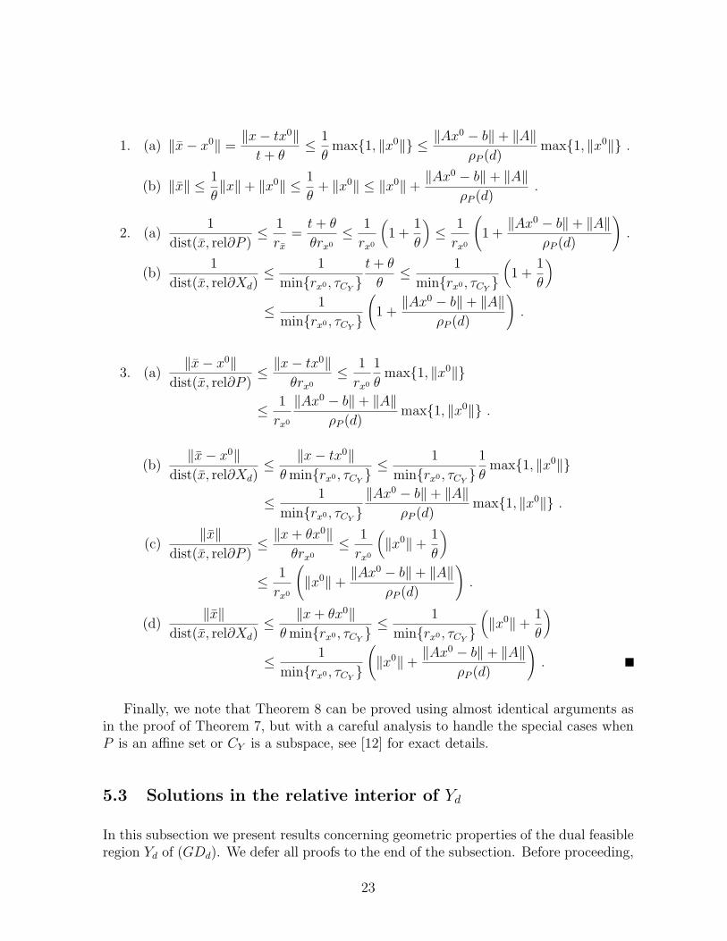
To finish the proof, we just have to bound the different expressions from the statementof the theorem; here we make use of inequality (24):
22
1. (a) ‖x− x0‖ =‖x− tx0‖
t + θ≤ 1
θmax{1, ‖x0‖} ≤ ‖Ax0 − b‖+ ‖A‖
ρP (d)max{1, ‖x0‖} .
(b) ‖x‖ ≤ 1
θ‖x‖+ ‖x0‖ ≤ 1
θ+ ‖x0‖ ≤ ‖x0‖+
‖Ax0 − b‖+ ‖A‖ρP (d)
.
2. (a)1
dist(x, rel∂P )≤ 1
rx
=t + θ
θrx0
≤ 1
rx0
(1 +
1
θ
)≤ 1
rx0
(1 +
‖Ax0 − b‖+ ‖A‖ρP (d)
).
(b)1
dist(x, rel∂Xd)≤ 1
min{rx0 , τCY}
t + θ
θ≤ 1
min{rx0 , τCY}
(1 +
1
θ
)
≤ 1
min{rx0 , τCY}
(1 +
‖Ax0 − b‖+ ‖A‖ρP (d)
).
3. (a)‖x− x0‖
dist(x, rel∂P )≤ ‖x− tx0‖
θrx0
≤ 1
rx0
1
θmax{1, ‖x0‖}
≤ 1
rx0
‖Ax0 − b‖+ ‖A‖ρP (d)
max{1, ‖x0‖} .
(b)‖x− x0‖
dist(x, rel∂Xd)≤ ‖x− tx0‖
θ min{rx0 , τCY}≤ 1
min{rx0 , τCY}
1
θmax{1, ‖x0‖}
≤ 1
min{rx0 , τCY}‖Ax0 − b‖+ ‖A‖
ρP (d)max{1, ‖x0‖} .
(c)‖x‖
dist(x, rel∂P )≤ ‖x + θx0‖
θrx0
≤ 1
rx0
(‖x0‖+
1
θ
)
≤ 1
rx0
(‖x0‖+
‖Ax0 − b‖+ ‖A‖ρP (d)
).
(d)‖x‖
dist(x, rel∂Xd)≤ ‖x + θx0‖
θ min{rx0 , τCY}≤ 1
min{rx0 , τCY}
(‖x0‖+
1
θ
)
≤ 1
min{rx0 , τCY}
(‖x0‖+
‖Ax0 − b‖+ ‖A‖ρP (d)
).
Finally, we note that Theorem 8 can be proved using almost identical arguments asin the proof of Theorem 7, but with a careful analysis to handle the special cases whenP is an affine set or CY is a subspace, see [12] for exact details.
5.3 Solutions in the relative interior of Yd
In this subsection we present results concerning geometric properties of the dual feasibleregion Yd of (GDd). We defer all proofs to the end of the subsection. Before proceeding,
23
we first discuss norms that arise when studying the dual problem. Motivated quitenaturally by (18), we define the norm ‖(x, t)‖ := ‖x‖+|t| for points (x, t) ∈ C ⊂ IRn×IR.This then leads to the following dual norm for points (s, u) ∈ C∗ ⊂ IRn × IR:
‖(s, u)‖∗ := max{‖s‖∗, |u|} . (25)
Consistent with the characterization of ρD(d) given by (20) in Theorem 6, we definethe following dual norm for points (y, δ) ∈ IRm × IR:
‖(y, δ)‖∗ := ‖y‖∗ + |δ| . (26)
It is clear that the above defines a norm on the vector space IRm× IR which contains Yd.
The following proposition bounds the norm of the y component of the dual feasiblesolution (y, u) in terms of the objective function value bty−u; it corresponds to Lemma3.1 of [16] for the ground-set model format.
Proposition 6 Consider any (y, u) feasible for (GDd). If ρP (d) > 0 then
‖y‖∗ ≤max {‖c‖∗,−(bty − u)}
ρP (d).
The following result corresponds to Assertion 1 of Theorem 1.1 of [16] for the ground-set model format dual problem (GDd):
Proposition 7 Consider any y0 ∈ C∗Y . If ρD(d) > 0 then for any ε > 0, there exists
(y, u) ∈ Yd satisfying
‖y − y0‖ ≤ dist(c− Aty0, R∗) + ε
ρD(d)max
{1, ‖y0‖
}.
The following is the main result of this subsection, and can be viewed as an extensionof Theorems 15, 17, and 19 of [8] to the dual problem (GDd). In Theorem 9 we assumefor expository convenience that CY is not a subspace and that R (the recession cone ofP ) is not a subspace. These assumptions are relaxed in Theorem 10.
Theorem 9 Suppose that R and CY are not subspaces and consider any y0 ∈ C∗Y . If
ρD(d) > 0 then for any ε > 0, there exists (y, u) ∈ Yd satisfying:
1. (a) ‖y − y0‖∗ ≤‖c− Aty0‖∗ + ‖A‖
ρD(d)max{1, ‖y0‖∗}
24
(b) ‖y‖∗ ≤ ‖y0‖∗ +‖c− Aty0‖∗ + ‖A‖
ρD(d)
2. (a)1
dist(y, rel∂C∗Y )
≤ 1
dist(y0, rel∂C∗Y )
(1 +
‖c− Aty0‖∗ + ‖A‖ρD(d)
)
(b)1
dist((y, u), rel∂Yd)≤ (1 + ε) max{1, ‖A‖}
min {dist(y0, rel∂C∗Y ), τR∗}
(1 +
‖c− Aty0‖∗ + ‖A‖ρD(d)
)
3. (a)‖y − y0‖∗
dist(y, rel∂C∗Y )
≤ 1
dist(y0, rel∂C∗Y )
(‖c− Aty0‖∗ + ‖A‖
ρD(d)max{1, ‖y0‖∗}
)
(b)‖y − y0‖∗
dist((y, u), rel∂Yd)≤
(1 + ε) max{1, ‖A‖}min {dist(y0, rel∂C∗
Y ), τR∗}
(‖c− Aty0‖∗ + ‖A‖
ρD(d)max{1, ‖y0‖∗}
)
(c)‖y‖∗
dist(y, rel∂C∗Y )
≤ 1
dist(y0, rel∂C∗Y )
(‖y0‖∗ +
‖c− Aty0‖∗ + ‖A‖ρD(d)
)
(d)‖y‖∗
dist((y, u), rel∂Yd)≤
(1 + ε) max{1, ‖A‖}min {dist(y0, rel∂C∗
Y ), τR∗}
(‖y0‖∗ +
‖c− Aty0‖∗ + ‖A‖ρD(d)
)
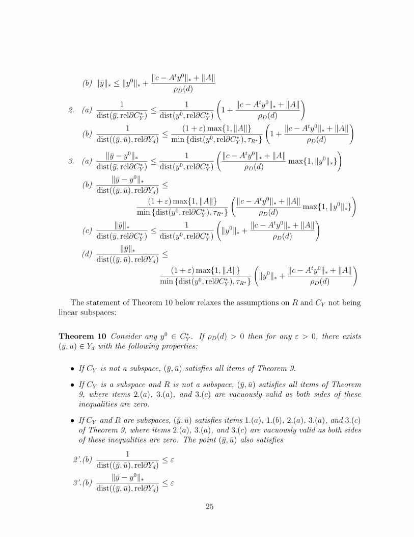
The statement of Theorem 10 below relaxes the assumptions on R and CY not beinglinear subspaces:
Theorem 10 Consider any y0 ∈ C∗Y . If ρD(d) > 0 then for any ε > 0, there exists
(y, u) ∈ Yd with the following properties:
• If CY is not a subspace, (y, u) satisfies all items of Theorem 9.
• If CY is a subspace and R is not a subspace, (y, u) satisfies all items of Theorem9, where items 2.(a), 3.(a), and 3.(c) are vacuously valid as both sides of theseinequalities are zero.
• If CY and R are subspaces, (y, u) satisfies items 1.(a), 1.(b), 2.(a), 3.(a), and 3.(c)of Theorem 9, where items 2.(a), 3.(a), and 3.(c) are vacuously valid as both sidesof these inequalities are zero. The point (y, u) also satisfies
2’.(b)1
dist((y, u), rel∂Yd)≤ ε
3’.(b)‖y − y0‖∗
dist((y, u), rel∂Yd)≤ ε
25
3’.(d)‖y‖∗
dist((y, u), rel∂Yd)≤ ε
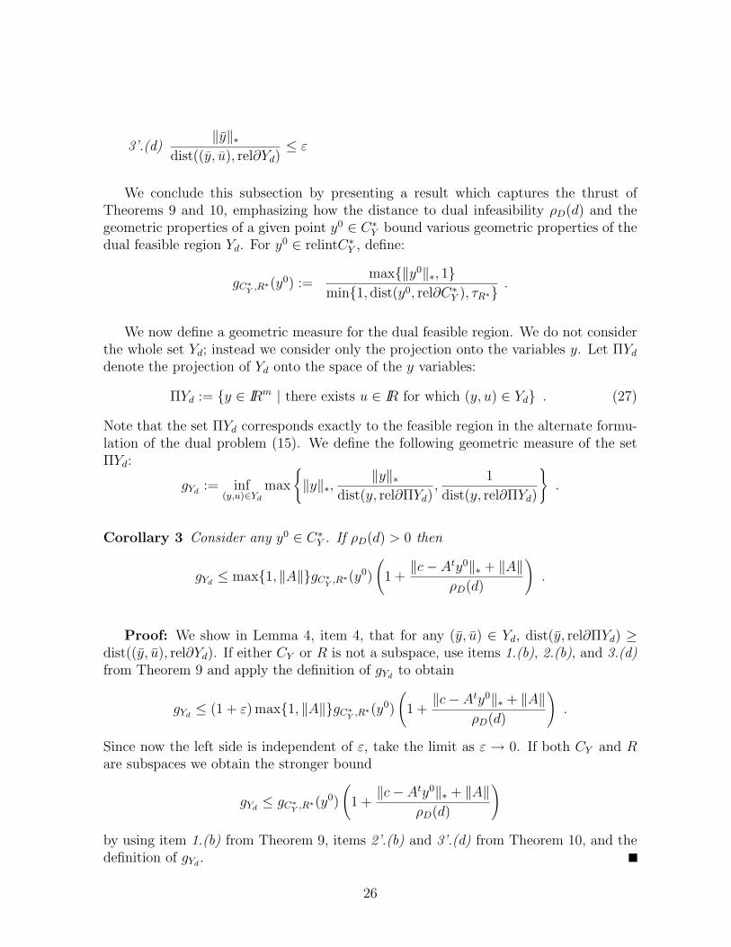
We conclude this subsection by presenting a result which captures the thrust ofTheorems 9 and 10, emphasizing how the distance to dual infeasibility ρD(d) and thegeometric properties of a given point y0 ∈ C∗
Y bound various geometric properties of thedual feasible region Yd. For y0 ∈ relintC∗
Y , define:
gC∗Y ,R∗(y0) :=
max{‖y0‖∗, 1}min{1, dist(y0, rel∂C∗
Y ), τR∗}.
We now define a geometric measure for the dual feasible region. We do not considerthe whole set Yd; instead we consider only the projection onto the variables y. Let ΠYd
denote the projection of Yd onto the space of the y variables:
ΠYd := {y ∈ IRm | there exists u ∈ IR for which (y, u) ∈ Yd} . (27)
Note that the set ΠYd corresponds exactly to the feasible region in the alternate formu-lation of the dual problem (15). We define the following geometric measure of the setΠYd:
gYd:= inf
(y,u)∈Yd
max
{‖y‖∗,
‖y‖∗dist(y, rel∂ΠYd)
,1
dist(y, rel∂ΠYd)
}.
Corollary 3 Consider any y0 ∈ C∗Y . If ρD(d) > 0 then
gYd≤ max{1, ‖A‖}gC∗
Y ,R∗(y0)
(1 +
‖c− Aty0‖∗ + ‖A‖ρD(d)
).
Proof: We show in Lemma 4, item 4, that for any (y, u) ∈ Yd, dist(y, rel∂ΠYd) ≥dist((y, u), rel∂Yd). If either CY or R is not a subspace, use items 1.(b), 2.(b), and 3.(d)from Theorem 9 and apply the definition of gYd
to obtain
gYd≤ (1 + ε) max{1, ‖A‖}gC∗
Y ,R∗(y0)
(1 +
‖c− Aty0‖∗ + ‖A‖ρD(d)
).
Since now the left side is independent of ε, take the limit as ε → 0. If both CY and Rare subspaces we obtain the stronger bound
gYd≤ gC∗
Y ,R∗(y0)
(1 +
‖c− Aty0‖∗ + ‖A‖ρD(d)
)
by using item 1.(b) from Theorem 9, items 2’.(b) and 3’.(d) from Theorem 10, and thedefinition of gYd
.
26
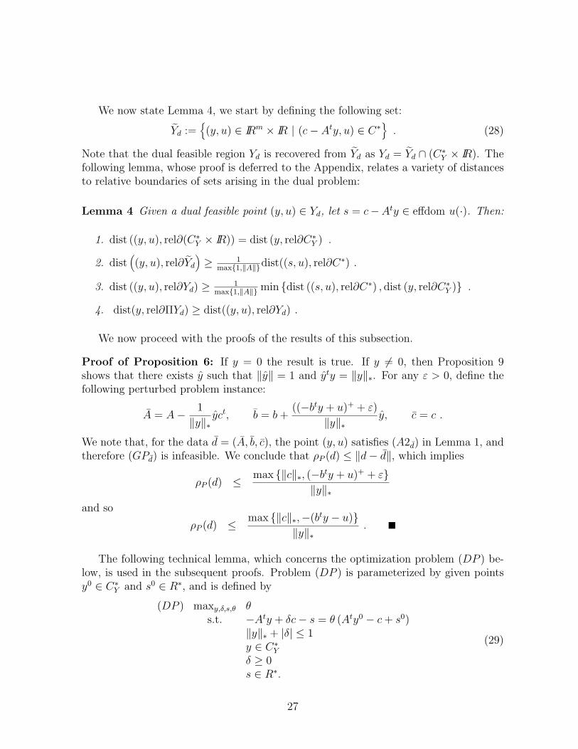
We now state Lemma 4, we start by defining the following set:
Yd :={(y, u) ∈ IRm × IR | (c− Aty, u) ∈ C∗
}. (28)
Note that the dual feasible region Yd is recovered from Yd as Yd = Yd ∩ (C∗Y × IR). The
following lemma, whose proof is deferred to the Appendix, relates a variety of distancesto relative boundaries of sets arising in the dual problem:
Lemma 4 Given a dual feasible point (y, u) ∈ Yd, let s = c−Aty ∈ effdom u(·). Then:
We now proceed with the proofs of the results of this subsection.
Proof of Proposition 6: If y = 0 the result is true. If y 6= 0, then Proposition 9shows that there exists y such that ‖y‖ = 1 and yty = ‖y‖∗. For any ε > 0, define thefollowing perturbed problem instance:
A = A− 1
‖y‖∗yct, b = b +
((−bty + u)+ + ε)
‖y‖∗y, c = c .
We note that, for the data d = (A, b, c), the point (y, u) satisfies (A2d) in Lemma 1, andtherefore (GPd) is infeasible. We conclude that ρP (d) ≤ ‖d− d‖, which implies
ρP (d) ≤ max {‖c‖∗, (−bty + u)+ + ε}‖y‖∗
and so
ρP (d) ≤ max {‖c‖∗,−(bty − u)}‖y‖∗
.
The following technical lemma, which concerns the optimization problem (DP ) be-low, is used in the subsequent proofs. Problem (DP ) is parameterized by given pointsy0 ∈ C∗
Y and s0 ∈ R∗, and is defined by
(DP ) maxy,δ,s,θ θs.t. −Aty + δc− s = θ (Aty0 − c + s0)
‖y‖∗ + |δ| ≤ 1y ∈ C∗
Y
δ ≥ 0s ∈ R∗.
(29)
27
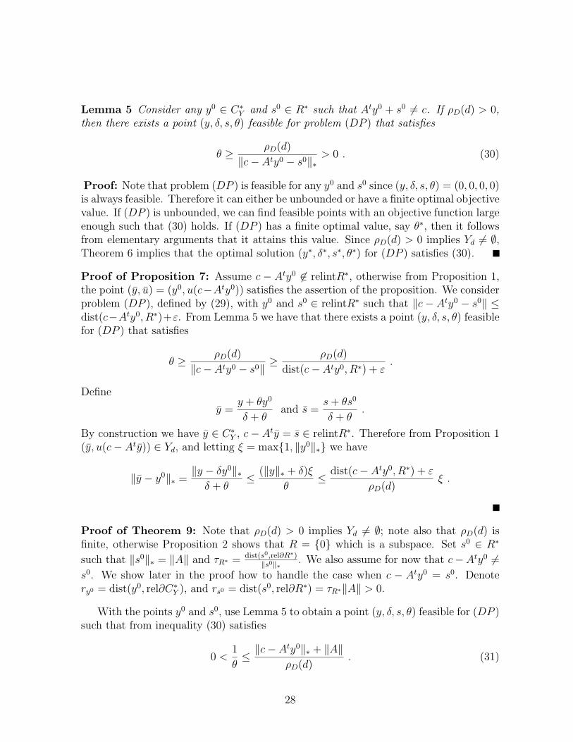
Lemma 5 Consider any y0 ∈ C∗Y and s0 ∈ R∗ such that Aty0 + s0 6= c. If ρD(d) > 0,
then there exists a point (y, δ, s, θ) feasible for problem (DP ) that satisfies
θ ≥ ρD(d)
‖c− Aty0 − s0‖∗> 0 . (30)
Proof: Note that problem (DP ) is feasible for any y0 and s0 since (y, δ, s, θ) = (0, 0, 0, 0)is always feasible. Therefore it can either be unbounded or have a finite optimal objectivevalue. If (DP ) is unbounded, we can find feasible points with an objective function largeenough such that (30) holds. If (DP ) has a finite optimal value, say θ∗, then it followsfrom elementary arguments that it attains this value. Since ρD(d) > 0 implies Yd 6= ∅,Theorem 6 implies that the optimal solution (y∗, δ∗, s∗, θ∗) for (DP ) satisfies (30).
Proof of Proposition 7: Assume c − Aty0 6∈ relintR∗, otherwise from Proposition 1,the point (y, u) = (y0, u(c−Aty0)) satisfies the assertion of the proposition. We considerproblem (DP ), defined by (29), with y0 and s0 ∈ relintR∗ such that ‖c− Aty0 − s0‖ ≤dist(c−Aty0, R∗)+ε. From Lemma 5 we have that there exists a point (y, δ, s, θ) feasiblefor (DP ) that satisfies
θ ≥ ρD(d)
‖c− Aty0 − s0‖≥ ρD(d)
dist(c− Aty0, R∗) + ε.
Define
y =y + θy0
δ + θand s =
s + θs0
δ + θ.
By construction we have y ∈ C∗Y , c− Aty = s ∈ relintR∗. Therefore from Proposition 1
(y, u(c− Aty)) ∈ Yd, and letting ξ = max{1, ‖y0‖∗} we have
‖y − y0‖∗ =‖y − δy0‖∗
δ + θ≤ (‖y‖∗ + δ)ξ
θ≤ dist(c− Aty0, R∗) + ε
ρD(d)ξ .
Proof of Theorem 9: Note that ρD(d) > 0 implies Yd 6= ∅; note also that ρD(d) isfinite, otherwise Proposition 2 shows that R = {0} which is a subspace. Set s0 ∈ R∗
such that ‖s0‖∗ = ‖A‖ and τR∗ = dist(s0,rel∂R∗)‖s0‖∗ . We also assume for now that c−Aty0 6=
s0. We show later in the proof how to handle the case when c − Aty0 = s0. Denotery0 = dist(y0, rel∂C∗
Y ), and rs0 = dist(s0, rel∂R∗) = τR∗‖A‖ > 0.
With the points y0 and s0, use Lemma 5 to obtain a point (y, δ, s, θ) feasible for (DP )such that from inequality (30) satisfies
0 <1
θ≤ ‖c− Aty0‖∗ + ‖A‖
ρD(d). (31)
28
Define the following:
y =y + θy0
δ + θ, s =
s + θs0
δ + θ, ry =
θry0
δ + θ, rs =
θrs0
δ + θ.
By construction dist(y, rel∂C∗Y ) ≥ ry, dist(s, rel∂R∗) ≥ rs, and c − Aty = s. There-
fore, from Proposition 1 the point (y, u(s)) ∈ Yd. We now choose u so that (y, u) ∈ Yd
and bound its distance to the relative boundary. Since relint R∗ ⊆ effdom u(·), from
Proposition 11 and Proposition 12, we have that for any ε > 0, the ball B(s, rs
1+ε
)∩LR∗ ⊂
relint effdom u(·). Define the function µ(·, ·) by
µ(s, κ) := 1‖A‖κ + sups u(s) .
‖s− s‖∗ ≤ κs ∈ R∗
Note that µ(·, ·) is finite for every s ∈ relint effdom u(·) and κ ∈ [0, dist(s, rel∂R∗)),because it is defined as the supremum of the continuous function u(·) over a closed andbounded subset contained in the relative interior of its effective domain, see Theorem10.1 of [18]. We define u = µ
(s, rs
1+ε
), and since u ≥ rs
‖A‖(1+ε)+ u(s) ≥ u(s) the
point (y, u) ∈ Yd. Let us now bound dist((y, u), rel∂Yd). Consider any vector v ∈LC∗
Y∩ {y| − Aty ∈ LR∗} such that ‖v‖∗ ≤ 1, then
y + αv ∈ C∗Y for any |α| ≤ ry ,
and
c− At(y + αv) = s + α(−Atv) ∈ B(s,
rs
1 + ε
)∩ LR∗ for any |α| ≤ rs
‖A‖(1 + ε).
This last inclusion implies that (c− At(y + αv), u + β) = (s + α(−Atv), u + β) ∈ C∗
for any |α|, |β| ≤ rs
‖A‖(1+ε). We have shown that dist(y, rel∂C∗
Y ) ≥ ry and dist((c −Aty, u), rel∂C∗) ≥ rs
‖A‖(1+ε). Therefore item 3 of Lemma 4 implies
dist((y, u), rel∂Yd) ≥ 1
max{1, ‖A‖}min
{ry,
rs
‖A‖(1 + ε)
}
≥ 1
(1 + ε) max{1, ‖A‖}θ
δ + θmin
{ry0 ,
rs0
‖A‖
}
=θ min{ry0 , τR∗}
(1 + ε) max{1, ‖A‖}(δ + θ).
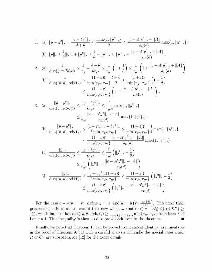
To finish the proof, we bound the different expressions in the statement of the theo-rem; let ξ = max{1, ‖A‖} to simplify notation. Here we use inequality (31):
29
1. (a) ‖y − y0‖∗ =‖y − δy0‖∗
δ + θ≤ max{1, ‖y0‖∗}
θ≤ ‖c− Aty0‖∗ + ‖A‖
ρD(d)max{1, ‖y0‖∗} .
(b) ‖y‖∗ ≤1
θ‖y‖∗ + ‖y0‖∗ ≤
1
θ+ ‖y0‖∗ ≤ ‖y0‖∗ +
‖c− Aty0‖∗ + ‖A‖ρD(d)
.
2. (a)1
dist(y, rel∂C∗Y )
≤ 1
ry
=δ + θ
θry0
≤ 1
ry0
(1 +
1
θ
)≤ 1
ry0
(1 +
‖c− Aty0‖∗ + ‖A‖ρD(d)
).
(b)1
dist((y, u), rel∂Yd)≤ (1 + ε)ξ
min{ry0 , τR∗}δ + θ
θ≤ (1 + ε)ξ
min{ry0 , τR∗}
(1 +
1
θ
)
≤ (1 + ε)ξ
min{ry0 , τR∗}
(1 +
‖c− Aty0‖∗ + ‖A‖ρD(d)
).
3. (a)‖y − y0‖∗
dist(y, rel∂C∗Y )
≤ ‖y − δy0‖∗θry0
≤ 1
ry0θmax{1, ‖y0‖∗}
≤ 1
ry0
‖c− Aty0‖∗ + ‖A‖ρD(d)
max{1, ‖y0‖∗} .
(b)‖y − y0‖∗
dist((y, u), rel∂Yd)≤ (1 + ε)ξ‖y − δy0‖∗
θ min{ry0 , τR∗}≤ (1 + ε)ξ
min{ry0 , τR∗}1
θmax{1, ‖y0‖∗}
≤ (1 + ε)ξ
min{ry0 , τR∗}‖c− Aty0‖∗ + ‖A‖
ρD(d)max{1, ‖y0‖∗} .
(c)‖y‖∗
dist(y, rel∂C∗Y )
≤ ‖y + θy0‖∗θry0
≤ 1
ry0
(‖y0‖∗ +
1
θ
)
≤ 1
ry0
(‖y0‖∗ +
‖c− Aty0‖∗ + ‖A‖ρD(d)
).
(d)‖y‖∗
dist((y, u), rel∂Yd)≤ ‖y + θy0‖∗(1 + ε)ξ
θ min{ry0 , τR∗}≤ (1 + ε)ξ
min{ry0 , τR∗}
(‖y0‖∗ +
1
θ
)
≤ (1 + ε)ξ
min{ry0 , τR∗}
(‖y0‖∗ +
‖c− Aty0‖∗ + ‖A‖ρD(d)
).
For the case c − Aty0 = s0, define y = y0 and u = µ(s0, τR∗‖A‖
1+ε
). The proof then
proceeds exactly as above, except that now we show that dist((c − Aty, u), rel∂C∗) ≥τR∗1+ε
, which implies that dist((y, u), rel∂Yd) ≥ 1max{1,‖A‖}(1+ε)
min{τR∗ , ry0} from item 3 ofLemma 4. This inequality is then used to prove each item in the theorem.
Finally, we note that Theorem 10 can be proved using almost identical arguments asin the proof of Theorem 9, but with a careful analysis to handle the special cases whenR or CY are subspaces, see [12] for the exact details.
30
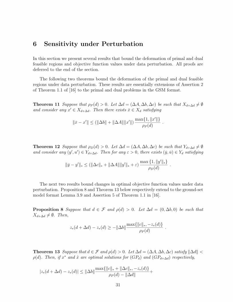
6 Sensitivity under Perturbation
In this section we present several results that bound the deformation of primal and dualfeasible regions and objective function values under data perturbation. All proofs aredeferred to the end of the section.
The following two theorems bound the deformation of the primal and dual feasibleregions under data perturbation. These results are essentially extensions of Assertion 2of Theorem 1.1 of [16] to the primal and dual problems in the GSM format.
Theorem 11 Suppose that ρP (d) > 0. Let ∆d = (∆A, ∆b, ∆c) be such that Xd+∆d 6= ∅and consider any x′ ∈ Xd+∆d. Then there exists x ∈ Xd satisfying
‖x− x′‖ ≤ (‖∆b‖+ ‖∆A‖‖x′‖) max{1, ‖x′‖}ρP (d)
.
Theorem 12 Suppose that ρD(d) > 0. Let ∆d = (∆A, ∆b, ∆c) be such that Yd+∆d 6= ∅and consider any (y′, u′) ∈ Yd+∆d. Then for any ε > 0, there exists (y, u) ∈ Yd satisfying
‖y − y′‖∗ ≤ (‖∆c‖∗ + ‖∆A‖‖y′‖∗ + ε)max {1, ‖y′‖∗}
ρD(d).
The next two results bound changes in optimal objective function values under dataperturbation. Proposition 8 and Theorem 13 below respectively extend to the ground-setmodel format Lemma 3.9 and Assertion 5 of Theorem 1.1 in [16].
Proposition 8 Suppose that d ∈ F and ρ(d) > 0. Let ∆d = (0, ∆b, 0) be such thatXd+∆d 6= ∅. Then,
z∗(d + ∆d)− z∗(d) ≥ −‖∆b‖max{‖c‖∗,−z∗(d)}ρP (d)
.
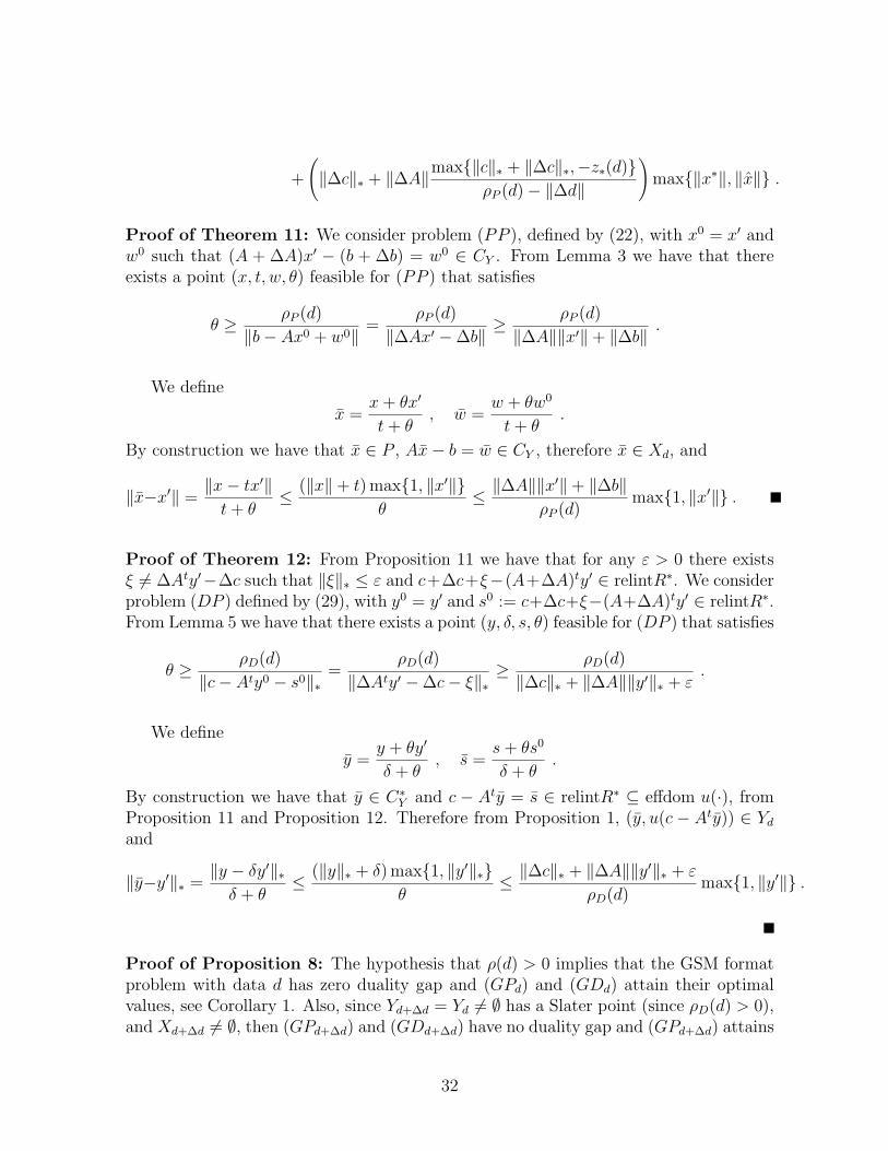
Theorem 13 Suppose that d ∈ F and ρ(d) > 0. Let ∆d = (∆A, ∆b, ∆c) satisfy ‖∆d‖ <ρ(d). Then, if x∗ and x are optimal solutions for (GPd) and (GPd+∆d) respectively,
Proof of Theorem 11: We consider problem (PP ), defined by (22), with x0 = x′ andw0 such that (A + ∆A)x′ − (b + ∆b) = w0 ∈ CY . From Lemma 3 we have that thereexists a point (x, t, w, θ) feasible for (PP ) that satisfies
θ ≥ ρP (d)
‖b− Ax0 + w0‖=
ρP (d)
‖∆Ax′ −∆b‖≥ ρP (d)
‖∆A‖‖x′‖+ ‖∆b‖.
We define
x =x + θx′
t + θ, w =
w + θw0
t + θ.
By construction we have that x ∈ P , Ax− b = w ∈ CY , therefore x ∈ Xd, and
‖x−x′‖ =‖x− tx′‖
t + θ≤ (‖x‖+ t) max{1, ‖x′‖}
θ≤ ‖∆A‖‖x′‖+ ‖∆b‖
ρP (d)max{1, ‖x′‖} .
Proof of Theorem 12: From Proposition 11 we have that for any ε > 0 there existsξ 6= ∆Aty′−∆c such that ‖ξ‖∗ ≤ ε and c+∆c+ξ−(A+∆A)ty′ ∈ relintR∗. We considerproblem (DP ) defined by (29), with y0 = y′ and s0 := c+∆c+ξ−(A+∆A)ty′ ∈ relintR∗.From Lemma 5 we have that there exists a point (y, δ, s, θ) feasible for (DP ) that satisfies
θ ≥ ρD(d)
‖c− Aty0 − s0‖∗=
ρD(d)
‖∆Aty′ −∆c− ξ‖∗≥ ρD(d)
‖∆c‖∗ + ‖∆A‖‖y′‖∗ + ε.
We define
y =y + θy′
δ + θ, s =
s + θs0
δ + θ.
By construction we have that y ∈ C∗Y and c − Aty = s ∈ relintR∗ ⊆ effdom u(·), from
Proposition 11 and Proposition 12. Therefore from Proposition 1, (y, u(c − Aty)) ∈ Yd
and
‖y−y′‖∗ =‖y − δy′‖∗
δ + θ≤ (‖y‖∗ + δ) max{1, ‖y′‖∗}
θ≤ ‖∆c‖∗ + ‖∆A‖‖y′‖∗ + ε
ρD(d)max{1, ‖y′‖} .
Proof of Proposition 8: The hypothesis that ρ(d) > 0 implies that the GSM formatproblem with data d has zero duality gap and (GPd) and (GDd) attain their optimalvalues, see Corollary 1. Also, since Yd+∆d = Yd 6= ∅ has a Slater point (since ρD(d) > 0),and Xd+∆d 6= ∅, then (GPd+∆d) and (GDd+∆d) have no duality gap and (GPd+∆d) attains
32
its optimal value, see Theorem 2. Let (y, u) ∈ Yd be an optimal solution of (GDd), dueto the form of the perturbation, point (y, u) ∈ Yd+∆d, and therefore
z∗(d + ∆d) ≥ (b + ∆b)t y − u = z∗(d) + ∆bty ≥ z∗(d)− ‖∆b‖‖y‖∗ .
The result now follows using the bound on the norm of dual feasible solutions fromProposition 6 and the strong duality for data instances d and d + ∆d.
Proof of Theorem 13: The hypothesis that ρ(d) > 0 and ρ(d + ∆d) > 0 imply thatthe GSM format problems with data d and d + ∆d both have zero duality gap and allproblems attain their optimal values, see Corollary 1.
Let x ∈ Xd+∆d be an optimal solution for (GPd+∆d). Define the perturbation ∆d =(0, ∆b−∆Ax, 0). Then by construction the point x ∈ Xd+∆d. Therefore
where x∗ ∈ Xd is an optimal solution for (GPs). The value −z∗(d+∆d) can be replacedby −z∗(d) on the right side of the previous bound. To see this consider two cases. If−z∗(d+∆d) ≤ −z∗(d), then we can do the replacement since it yields a larger bound. If−z∗(d+∆d) > −z∗(d), the inequality above has a negative left side and a positive rightside after the replacement. Note also that because of the hypothesis ‖∆d‖ < ρ(d), thedistance to infeasibility satisfies ρP (d + ∆d) ≥ ρP (d) − ‖∆d‖ > 0. We finish the proofcombining the previous two bounds, incorporating the lower bound on ρP (d + ∆d), andusing strong duality of the data instances d and d + ∆d.
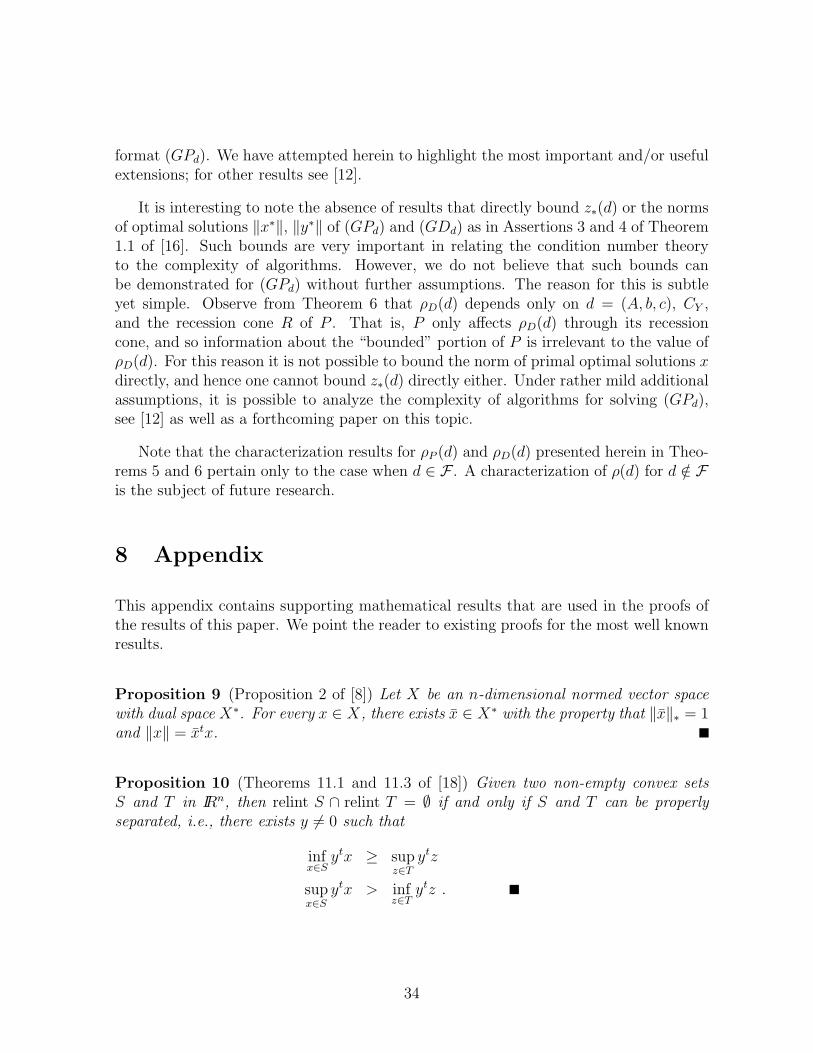
7 Concluding Remarks
We have shown herein that most of the essential results regarding condition numbers forconic convex optimization problems can be extended to the non-conic ground-set model
33
format (GPd). We have attempted herein to highlight the most important and/or usefulextensions; for other results see [12].
It is interesting to note the absence of results that directly bound z∗(d) or the normsof optimal solutions ‖x∗‖, ‖y∗‖ of (GPd) and (GDd) as in Assertions 3 and 4 of Theorem1.1 of [16]. Such bounds are very important in relating the condition number theoryto the complexity of algorithms. However, we do not believe that such bounds canbe demonstrated for (GPd) without further assumptions. The reason for this is subtleyet simple. Observe from Theorem 6 that ρD(d) depends only on d = (A, b, c), CY ,and the recession cone R of P . That is, P only affects ρD(d) through its recessioncone, and so information about the “bounded” portion of P is irrelevant to the value ofρD(d). For this reason it is not possible to bound the norm of primal optimal solutions xdirectly, and hence one cannot bound z∗(d) directly either. Under rather mild additionalassumptions, it is possible to analyze the complexity of algorithms for solving (GPd),see [12] as well as a forthcoming paper on this topic.
Note that the characterization results for ρP (d) and ρD(d) presented herein in Theo-rems 5 and 6 pertain only to the case when d ∈ F . A characterization of ρ(d) for d /∈ Fis the subject of future research.
8 Appendix
This appendix contains supporting mathematical results that are used in the proofs ofthe results of this paper. We point the reader to existing proofs for the most well knownresults.
Proposition 9 (Proposition 2 of [8]) Let X be an n-dimensional normed vector spacewith dual space X∗. For every x ∈ X, there exists x ∈ X∗ with the property that ‖x‖∗ = 1and ‖x‖ = xtx.
Proposition 10 (Theorems 11.1 and 11.3 of [18]) Given two non-empty convex setsS and T in IRn, then relint S ∩ relint T = ∅ if and only if S and T can be properlyseparated, i.e., there exists y 6= 0 such that
infx∈S
ytx ≥ supz∈T
ytz
supx∈S
ytx > infz∈T
ytz .
34
The following is a restatement of Corollary 14.2.1 of [18], which relates the effectivedomain of u(·) of (14) to the recession cone of P , where recall that R∗ denotes the dualof the recession cone R defined in (8).
Proposition 11 (Corollary 14.2.1 of [18]) Let R denote the recession cone of the nonemptyconvex set P , and define u(·) by (14). Then cl effdom u(·) = R∗.
Proposition 12 (Theorem 6.3 of [18]) For any convex set Q ⊆ IRn, cl relint Q = cl Q,and relint cl Q = relint Q.
The following lemma is central in relating the two alternative characterizations ofthe distance to infeasibility and is used in the proofs in Section 4.
Lemma 6 Consider two closed convex cones C ⊆ IRn and CY ⊆ IRm, and data (M, v) ∈IRm×n × IRm. Strong duality holds between
(P ) : z∗ = min ‖M ty + q‖∗ and (D) : z∗ = max θs.t. ytv ≥ 1 s.t. Mx− θv ∈ CY
y ∈ C∗Y ‖x‖ ≤ 1
q ∈ C∗ θ ≥ 0x ∈ C .
Proof: The proof that weak duality holds between (P ) and (D) is straightforward,therefore z∗ ≤ z∗. Assume z∗ < z∗, and set ε > 0 such that 0 ≤ z∗ < z∗ − ε. Considerthe following nonempty convex set S:
S :={(u, δ, α) | ∃y, q s.t. y + u ∈ C∗
Y , q + δ ∈ C∗, ytv ≥ 1− α, ‖M ty + q‖∗ ≤ z∗ − ε}
.
Then (0, 0, 0) /∈ S, and from Proposition 10 there exists (z, x, θ) 6= 0 such that ztu +xtδ + θα ≥ 0 for any (u, δ, α) ∈ S. For any y ∈ IRm, u ∈ C∗
Y , δ ∈ C∗, π ≥ 0, and q suchthat ‖q‖∗ ≤ z∗ − ε, define q = −M ty + q, u = −y + u, δ = −q + δ, and α = 1− ytv + π.This construction implies that the point (u, δ, α) ∈ S, and that for all y, u ∈ C∗
Y ,δ ∈ C∗, π ≥ 0, and ‖q‖∗ ≤ z∗ − ε it holds that:
0 ≤ zt(−y + u) + xt(M ty − q + δ) + θ(1− ytv + π)
= yt (Mx− θv − z) + ztu + xtδ − xtq + θ + θπ .
This implies that Mx − θv = z ∈ CY , x ∈ C, θ ≥ 0, and θ ≥ xtq for ‖q‖∗ ≤ z∗ − ε. Ifx 6= 0, re-scale (z, x, θ) such that ‖x‖ = 1 and then (x, θ) is feasible for (D). Set q =(z∗−ε)q, where q is given by Proposition 9 and is such that ‖q‖∗ = 1 and qtx = ‖x‖ = 1.It then follows that z∗ ≥ θ ≥ xtq = z∗ − ε > z∗, which is a contradiction.
35
If x = 0, the above expression implies −θv = z ∈ CY , and θ ≥ 0. If θ > 0 then−v ∈ CY , which means that the point (0, β) is feasible for (D) for any β ≥ 0, implyingthat z∗ = ∞, a contradiction since z∗ < z∗. If θ = 0, then z = 0, which is a contradictionsince (z, x, θ) 6= 0.
The next two lemmas concern properties of the distance to the relative boundary ofa convex set.
Lemma 7 Given convex sets A and B, and a point x ∈ A ∩B, then
dist(x, rel∂(A ∩B)) ≥ min {dist(x, rel∂A), dist(x, rel∂B)} .
Proof: The proof of this lemma is based in showing that LA∩B \ (A∩B) ⊂ (LA \ A)∪(LB \B). If this inclusion is true then
dist(x, rel∂(A ∩B)) = infx∈LA∩B\(A∩B)
‖x− x‖
≥ infx∈(LA\A)∪(LB\B)
‖x− x‖
= min
{inf
x∈LA\A‖x− x‖, inf
x∈LB\B‖x− x‖
}= min {dist(x, rel∂A), dist(x, rel∂B)} ,
which proves the lemma. Therefore we now prove the inclusion. Consider some x ∈LA∩B, this means that there exists αi ∈ IR, xi ∈ A∩B, i ∈ I a finite set, and
∑i∈I αi = 1,
such that x =∑
i∈I αixi. Since xi ∈ A and xi ∈ B, we have that x ∈ LA and x ∈ LB.Therefore LA∩B ⊂ LA∩LB. The desired inclusion is then obtained with a little algebra:
LA∩B \ (A ∩B) ⊂ LA ∩ LB ∩ (A ∩B)C
= LA ∩ LB ∩(AC ∪BC
)=
(LA ∩ LB ∩ AC
)∪(LA ∩ LB ∩BC
)⊂
(LA ∩ AC
)∪(LB ∩BC
)= (LA \ A) ∪ (LB \B) .
Last of all, we have:
Proof of Lemma 4: Equality (1.) is a consequence of the fact that (y, u) ∈ LC∗Y ×IR \
(C∗Y × IR) if and only if y ∈ LC∗
Y\C∗
Y , and that ‖(y, u)− (y, u)‖∗ = ‖y− y‖∗ + |u− u| =‖y − y‖∗.
To prove inequality (2.), we first show that if (y, u) ∈ LYd\ Yd, then (c − Aty, u) ∈
LC∗ \ C∗. First note that if (y, u) 6∈ Yd then, by the definition of Yd, (c− Aty, u) 6∈ C∗;
36
therefore we only need to show that if (y, u) ∈ LYd
then (c − Aty, u) ∈ LC∗ . Let
(y, u) ∈ LYd
. Then there exists αi ∈ IR, (yi, ui) ∈ Yd, i ∈ I a finite set, and∑
i∈I αi = 1,
such that (y, u) =∑
i∈I αi(yi, ui). Consider
(c− Aty, u) = (c− At∑i∈I
αiyi,∑i∈I
αiui) =∑i∈I
αi(c− Atyi, ui) .
Since (yi, ui) ∈ Yd then (c− Atyi, ui) ∈ C∗ and therefore (c− Aty, u) ∈ LC∗ .
The inclusion above means that
dist((s, u), rel∂C∗) = inf(s,u)∈LC∗\C∗
‖(s, u)− (s, u)‖∗
≤ inf(y,u)∈L
Yd\Yd
‖(s, u)− (c− Aty, u)‖∗
= inf(y,u)∈L
Yd\Yd
max{‖s− (c− Aty)‖∗, |u− u|}
= inf(y,u)∈L
Yd\Yd
max{‖Aty − Aty‖∗, |u− u|}
≤ inf(y,u)∈L
Yd\Yd
max{‖A‖‖y − y‖∗, |u− u|}
≤ inf(y,u)∈L
Yd\Yd
max{‖A‖, 1}max{‖y − y‖∗, |u− u|}
≤ max{‖A‖, 1} inf(y,u)∈L
Yd\Yd
(‖y − y‖∗ + |u− u|)
= max{‖A‖, 1} inf(y,u)∈L
Yd\Yd
‖(y, u)− (y, u)‖∗
= max{‖A‖, 1}dist((y, u), rel∂Yd) .
Inequality (3.) follows from the observation that Yd = Yd ∩ (C∗Y × IR), Lemma 7, and
the bounds obtained in (1.) and (2.).
The proof of item (4.) uses the fact (soon to be proved) that if y ∈ LΠYd\ ΠYd then
for any u, (y, u) ∈ LYd\ Yd. Then from the definition of the relative distance to the
boundary we have
dist ((y, u), rel∂Yd) = inf(y,u)∈LYd
\Yd
‖(y, u)− (y, u)‖∗
≤ infy∈LΠYd
\ΠYd,u‖(y, u)− (y, u)‖∗
= infy∈LΠYd
\ΠYd,u‖y − y‖∗ + |u− u|
= infy∈LΠYd
\ΠYd
‖y − y‖∗
= dist (y, rel∂ΠYd) ,
37
which proves inequality (4.). To finish the proof we now show that if y ∈ LΠYd\ ΠYd
then for any u, (y, u) ∈ LYd\ Yd. The fact that y 6∈ ΠYd implies that for any u,
(y, u) 6∈ Yd. Now since y ∈ LΠYd, there exists αi ∈ IR, (yi, ui) ∈ Yd, i ∈ I a finite set
such that y =∑
i∈I αiyi and∑
i∈I αi = 1. Since for any (y, u) ∈ Yd and β ≥ 0 the point(y, u + β) ∈ Yd, we can express the point (y, u) by the following sum of points in Yd
(y, u) =
(∑i∈I
αiyi + y − y,∑i∈I
αiui + u + β1 − u− β2
),
where for any u, β1 = (u−∑i∈I αiui)
+ and β2 = (u−∑i∈I αiui)
−. This shows that forany u, (y, u) ∈ LYd
, completing the proof.
References
[1] M. S. Bazaraa, H. D. Sherali, and C. M. Shetty. Nonlinear Programming, Theoryand Algorithms. John Wiley & Sons, Inc, New York, second edition, 1993.
[2] F. Cucker and J. Pena. A primal-dual algorithm for solving polyhedral conic systemswith a finite-precision machine. Technical report, GSIA, Carnegie Mellon University,2001.
[3] M. Epelman and R. M. Freund. A new condition measure, preconditioners, andrelations between different measures of conditioning for conic linear systems. SIAMJournal on Optimization, 12(3):627–655, 2002.
[4] S. Filipowski. On the complexity of solving sparse symmetric linear programs spec-ified with approximate data. Mathematics of Operations Research, 22(4):769–792,1997.
[5] S. Filipowski. On the complexity of solving feasible linear programs specified withapproximate data. SIAM Journal on Optimization, 9(4):1010–1040, 1999.
[6] R. M. Freund and J. R. Vera. Condition-based complexity of convex optimizationin conic linear form via the ellipsoid algorithm. SIAM Journal on Optimization,10(1):155–176, 1999.
[7] R. M. Freund and J. R. Vera. On the complexity of computing estimates of conditionmeasures of a conic linear system. Technical Report, Operations Research Center,MIT, August 1999.
[8] R. M. Freund and J. R. Vera. Some characterizations and properties of the “distanceto ill-posedness” and the condition measure of a conic linear system. MathematicalProgramming, 86(2):225–260, 1999.
38
[9] J. L. Goffin. The relaxation method for solving systems of linear inequalities. Math-ematics of Operations Research, 5(3):388–414, 1980.
[10] M. A. Nunez and R. M. Freund. Condition measures and properties of the centraltrajectory of a linear program. Mathematical Programming, 83(1):1–28, 1998.
[11] M. A. Nunez and R. M. Freund. Condition-measure bounds on the behavior ofthe central trajectory of a semi-definite program. SIAM Journal on Optimization,11(3):818–836, 2001.
[12] F. Ordonez. On the Explanatory Value of Condition Numbers for Convex Optimiza-tion: Theoretical Issues and Computational Experience. PhD thesis, MassachusettsInstitute of Technology, 2002.
[13] F. Ordonez and R. M. Freund. Computational experience and the explanatoryvalue of condition measures for linear optimization. Working Paper OR361-02,MIT, Operations Research Center, 2002.
[14] J. Pena. Computing the distance to infeasibility: theoretical and practical issues.Technical report, Center for Applied Mathematics, Cornell University, 1998.
[15] J. Pena and J. Renegar. Computing approximate solutions for convex conic systemsof constraints. Mathematical Programming, 87(3):351–383, 2000.
[16] J. Renegar. Some perturbation theory for linear programming. Mathematical Pro-gramming, 65(1):73–91, 1994.
[17] J. Renegar. Linear programming, complexity theory, and elementary functionalanalysis. Mathematical Programming, 70(3):279–351, 1995.
[18] R. T. Rockafellar. Convex Analysis. Princeton University Press, Princeton, NewJersey, 1997.
[19] J. R. Vera. Ill-posedness and the computation of solutions to linear programs withapproximate data. Technical Report, Cornell University, May 1992.
[20] J. R. Vera. Ill-Posedness in Mathematical Programming and Problem Solving withApproximate Data. PhD thesis, Cornell University, 1992.
[21] J. R. Vera. Ill-posedness and the complexity of deciding existence of solutions tolinear programs. SIAM Journal on Optimization, 6(3):549–569, 1996.
[22] J. R. Vera. On the complexity of linear programming under finite precision arith-metic. Mathematical Programming, 80(1):91–123, 1998.