Page 1
On an off-shore pipe laying problem
Citation for published version (APA):Mattheij, R. M. M., & Rienstra, S. W. (1987). On an off-shore pipe laying problem. (WD report; Vol. 8707).Nijmegen: Radboud Universiteit Nijmegen.
Document status and date:Published: 01/01/1987
Document Version:Publisher’s PDF, also known as Version of Record (includes final page, issue and volume numbers)
Please check the document version of this publication:
• A submitted manuscript is the version of the article upon submission and before peer-review. There can beimportant differences between the submitted version and the official published version of record. Peopleinterested in the research are advised to contact the author for the final version of the publication, or visit theDOI to the publisher's website.• The final author version and the galley proof are versions of the publication after peer review.• The final published version features the final layout of the paper including the volume, issue and pagenumbers.Link to publication
General rightsCopyright and moral rights for the publications made accessible in the public portal are retained by the authors and/or other copyright ownersand it is a condition of accessing publications that users recognise and abide by the legal requirements associated with these rights.
• Users may download and print one copy of any publication from the public portal for the purpose of private study or research. • You may not further distribute the material or use it for any profit-making activity or commercial gain • You may freely distribute the URL identifying the publication in the public portal.
If the publication is distributed under the terms of Article 25fa of the Dutch Copyright Act, indicated by the “Taverne” license above, pleasefollow below link for the End User Agreement:
www.tue.nl/taverne
Take down policyIf you believe that this document breaches copyright please contact us at:
[email protected]
providing details and we will investigate your claim.
Download date: 28. Dec. 2019
Page 2
Report WD 87-07
On An Off-Shore Pipe Laying Problem
R.M.M. Mattheij
S.W. Rienstra
August 1987
Wiskuhdige Dienstverlening Faculteit der Wiskunde en Natuurwetenschappen Katholieke Universiteit Toernooiveld 6525 ED Nijmegen The Netherlands
Page 3
ON AN OFF-SHORE PIPE LAYING PROBLEM
R.M.M. Mattheij S.W. Rienstra
The final version of this paper will be submitted for publication elsewhere
Page 4
Abstract
In this paper we consider a model for determining the shape of a pipe laid by a barge. We investigate
how the solution of a resulting second order non-linear differential equation depends critically on the
(unknown) vertical bottom reaction force; by this we can explain some difficulties met when approximating
the solution numerically. An important part of the analysis is based on studying a pendulum analogy in
a time dependent gravity field, by which we obtain existence and uniqueness results.
1. Introduction
The transportation of gas or oil from offshore wells requires the installation of pipelines to connect
the well to some mainland station.Typically such pipes are 16-36 inch in diameter and may be up to
several hundreds of kilometers long. Usually these pipes are laid in relatively shallow (""' 50 m) and deep
(-300m) water, although recently technology has been developed to handle very deep water (300-1000
m and more). Part of the technology is in the material of which the pipes are being made (high quality
steel), but very much depends on the laying technique too. The main problem to be dealt with is buckling
due to too high bending stresses during laying; pipe collapse due to a too high water pressure becomes
also important at greater depths, but we shall not consider that problem here.
At present the pipes are being laid using a so called laybarge where the pipe sections are welded
together, and then gradually released off the barge to the sea bed. If the welding ramp is horizontally
positioned, the pipe is released via a (circular) stinger. According to the shape of the suspended pipeline
this technique is called S-lay. If the welding ramp is in vertical position the technique is called J -lay.
Here we shall concentrate (although not in principle) on the S-lay technique, which is the usual one for
not very deep water. The analysis we give below is equally applicable for J -lay configurations though.
Usually, the pipes are relatively thin-walled and, without additional weight, would float on the water.
This weight is provided by application of a concrete coating, giving the pipes a net specific gravity of
about 1.05 to 1.30 times that of water. (The value depends on the product to be transported, and the
1
Page 5
presence of sea currents.) This non-negligible own weight, especially in deep water, tends to give the
pipe during laying a shape with such a high curvature, that without precautions the pipe would buckle.
Therefore, the laybarge is equipped with tension machines to apply a certain horizontal tension, just
sufficient to stretch the S curve and reduce the bending stresses to a safe level.
The practical question now is: given a certain geometry, how much tension is needed and, further
more, which is the optimal position of the stringer. On the one hand, repairing a buckled pipe is very
expensive, but on the other hand, so are the tension machines and other equipment, so rather accurate
calculations are required. Given the large number of parameters involved this problem has to be solved
again for each new case, and a mathematical model including a computer program is obviously required
(Ref. 1,2,3,4,5,6,7,8,9). This will be the subject of the present paper.
The problem as such arose from requests from offshore companies, who were interested in a routine
efficient and fast enough for a small computer, to be used on board in order to be able to respond
immediately to unforeseen variations in (e.g.) steel quality, concrete quality, or other problem parameters.
In trying to develop a program we hit severe numerical problems. In particular, since the problem is
nonlinear, we were often not able to make the Newton method involved converge. In search for the
phenomena behind this problem we encountered some interesting mathematical questions. An explanation
of the aforementioned problem was the presence of a 'dose' family of other solutions. We shall treat this
problem to some extent as we believe that it nicely demonstrates why numerical black boxes should be
treated with great care, also in industrial problems; another reason is that the fairly messy nonlinear
structure is elucidated substantially by invoking a mechanical analogy (§3). The existence of the desired
solution as a limiting case of the family of dose solutions is treated in §4. Finally, in §5 we consider some
more mathematical questions, arsising as mere off shoots, in particular concerning the bending energy.
2. The model
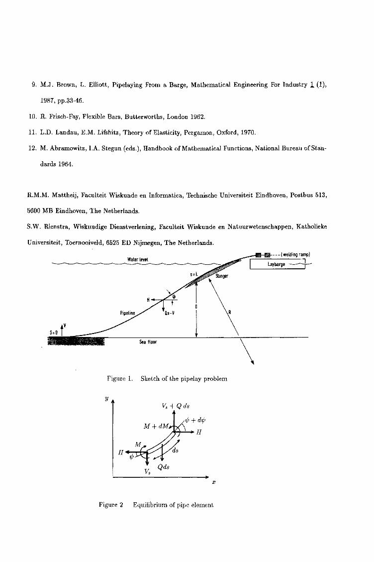
In this section we shall derive a model for the problem outlined above and indicate some questions
related to this problem. In figure 1 we have sketched the configuration of a laybarge. The pipe is guided
2
Page 6
into the water by a stinger having a certain uniform (adjustable) radius of curvature R. Typically three
forces are exerted on the pipe: a) gravity, due to the not negligible net weight, b) a horizontal tension
H, applied by the tension machines mounted on the vessel which is supposedly anchored, and c) the
(unknown) vertical bottom reaction force V.
By denoting:
s = arclength
Q effective pipe weight per unit length (2.1)
M = bending moment
E I = flexural rigidity
we have (Fig.2; cf. ref. 10,11)
(2.2a)
(2.2b)
(2.2c)
(2.2d)
M = EI d'ljJ (Bernoulli- Euler law) ds
d:: = H sin 'ljJ - V. cos '1/J (equilibrium of moments)
~~ = 0 (horizontal tension remains constant)
dV. = Q. ds
From (2.2) we derive the basic equation
(2.3) EI ~~ = Hsin'ljl- (Qs V)cos'ljJ
where we note that
z(s) = 111
cos'ljlds', y(s) = 1• sin'ljlds'.
Besides '1/J and V, also the free length L (from bottom to stinger departure point) is unknown. This
requires four boundary conditions in total to be specified. The ones we will adopt here are not ex-
actly corresponding to the configuration as drawn in fig.l (which would include a free boundary at the
3
Page 7
stinger, cf. ref.8), but somewhat simplified, however, without altering the characteristics of the problems
discussed.
We will consider in principle:
(2.4a) t,b(O)
(2.4b)
(2.4c)
0, dt,b(O) = 0 {free end supported by the bottom) ds
dt,b(L) = - Rl (stinger curvature) ds
foL sin t,b(s) ds = D (the total depth)
We now like to find the shape of the pipe, given a horizontal force H. This force is needed to give
the pipe a low enough curvature to prevent it from buckling. This buckling usually happens when the
combined stress due to bending, tension, and water pressure exceeds the yield stress, i.e., the maximal
stress that the steel can afford without plastic deformation.
We first reduce the problem parameters to a basic set. Introduce dimensionless quantities
(2.5a) t =sf Do, 1 = L/Do, d = D/Do
{2.5b) h = HD5/EI, q = QDgjEI, v = VDJ/EI
For convenience we introduced an unspecified length D0 , in order to prevent limiting cases as Q = 0,
H = 0, L -+ oo, D-+ oo to produce artificially singular, and therefore less interpretable problems. So
in general the number of dimensionless parameters may be reduced by one, and we may assume, for
example, h = 1 or q = 1. So we obtain
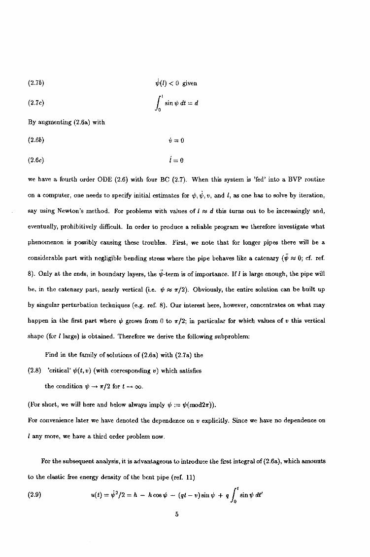
(2.6a) iP = h sin'¢- (qt- v) cos t,b
with boundary conditions
(2.7a) t,b(O) = o, ,P(o) = o
4
Page 8
(2.7b)
(2.7c)
By augmenting (2.6a) with
(2.6b)
(2.6c)
~(l) < 0 given
11
sin t/J dt = d
we have a fourth order ODE (2.6) with four BC (2.7). When this system is 'fed' into a BVP routine
on a computer, one needs to specify initial estimates for t/J, ~' v, and I, as one has to solve by iteration,
say using Newton's method. For problems with values of 1 ~ d this turns out to be increasingly and,
eventually, prohibitively difficult. In order to produce a reliable program we therefore investigate what
phenomenon is possibly causing these troubles. First, we note that for longer pipes there will be a
considerable part with negligible bending stress where the pipe behaves like a catenary ( ;fi ~ 0; cf. ref.
8). Only at the ends, in boundary layers, the ;fi-term is of importance. If I is large enough, the pipe will
be, in the catenary part, nearly vertical (i.e. t/J ~ 7r/2). Obviously, the entire solution can be built up
by singular perturbation techniques (e.g. ref. 8). Our interest here, however, concentrates on what may
happen in the first part where tP grows from 0 to 1r /2; in particular for which values of v this vertical
shape (for /large) is obtained. Therefore we derive the following subproblem:
Find in the family of solutions of (2.6a) with (2.7a) the
(2.8) 'critical' t/J(t,v) (with corresponding v) which satisfies
the condition tP --+ 1r /2 for t -+ oo.
(For short, we will here and below always imply tP := t/;(mod21r)).
For convenience later we have denoted the dependence on v explicitly. Since we have no dependence on
1 any more, we have a third order problem now.
For the subsequent analysis, it is advantageous to introduce the first integral of (2.6a), which amounts
to the elastic free energy density of the bent pipe (ref. 11)
(2.9) u(t)=~2/2=h- hcost/J- (qt-v)sint/J + q 1tsin¢dt'
5
Page 9
The total energy is then
(2.10) E = loo u( t)dt
Intuitively we may expect the problem (2.8) not to have a unique solution (and, likewise, also (2.6),
(2.7)), as the pipe could possibly make several bends and loops. In fig. 3 we have given some indication
of the intrinsical behaviour of t/J (in cartesian coordinates) for various values of v. This observation is the
clue to the numerical difficulties mentioned earlier: we shall show that the most natural solution of (2.8)
(with a minimal energy E) is dense in a family of solutions which are, at least numerically, close to the
required one of (2.6) with (2.7) if dis large. This then explains why it is hard, sometimes impossible, to
single out the desired one. To do this we shall employ a useful analogy which is introduced in the next
section.
3. Pendulum analogy
The variety and character of the solutions of (2.6a) would be much easier predicted and classified if
we can find an analogous problem, described by the same equation, but easier interpretable.
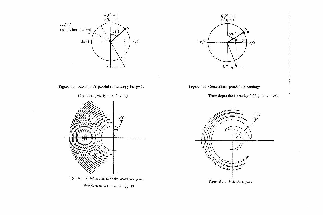
If q = 0 such an analogy exists indeed, and is actually a classic result due to Kirchhoff {cf. ref.lO).
It consists of a mathematical pendulum in a gravity field ( -h, v), where '1/J now denotes the angle of the
pendulum with the positive y-axis, and t is time; (fig. 4a). For given v, t/J will oscillate between tP = 0
and its mirror in the line (-h, v): '1/J = 211" 2 arctg(v/h). If v = 0 the pendulum will remain stationary
in its (unstable) initial position '1/J = 0, as the oscillation period tends to infinity for v-+ 0.
For q :f. 0 it is possible to generalise the pendulum analogy if we use a more general (admittedly
more artificial) time dependent gravity field ( -h, v- qt); (fig. 4b ). Then, as long as v- qt > 0, the force
field is directed to the right half (i.e. x > 0), and t/J will tend to return to the interval (0, 1r); however,
once v - qt has changed sign and increases with t without bound in negative direction, the force field
points to the left, and, as time increases, forces '1/J to remain in a decreasing interval around tP = 311" /2;
{fig. 5a). If vis large, this process takes some time, and t/J starts to oscillate around tP = 11"/2; (fig. 5b).
6
Page 10
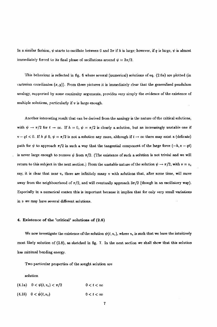
In a similar fashion, 1/J starts to oscillate between 0 and 21f if his large; however, if q is large, 1/J is almost
immediately forced to its final phase of oscillations around 1/J = 31f /2.
This behaviour is reflected in fig. 6 where several (numerical) solutions of eq. (2.6a) are plotted (in
cartesian coordinates ( :r:, y)). From these pictures it is immediately dear that the generalised pendulum
analogy, supported by some continuity arguments, provides very simply the evidence of the existence of
multiple solutions, particularly if v is large enough.
Another interesting result that can be derived from the analogy is the nature of the critical solutions,
with ,P __. 1rj2 fort _. oo. If h = 0, ¢ = 1rj2 is clearly a solution, but an increasingly unstable one if
v- qt < 0. If h =f. 0, ¢ = 1rj2 is not a solution any more, although if t __. oo there may exist a (delicate)
path for ¢ to approach 1r /2 in such a way that the tangential component of the large force ( -h, v - qt)
is never large enough to remove ¢ from 1r /2. (The existence of snch a solution is not trivial and we will
return to this subject in the next section.) From the unstable nature of the solution¢_. 1rj2, with v = Ve
say, it is clear that near Ve there are infinitely many v with solutions that, aft.er some time, will move
away from the neighbourhood of 1rj2, and will eventually approach 31f/2 (though in an oscillatory way).
Especially in a numerical contex this is important because it implies that for only very small variations
in v we may have several different solutions.
4. Existence of the 'critical' solutions of (2.8)
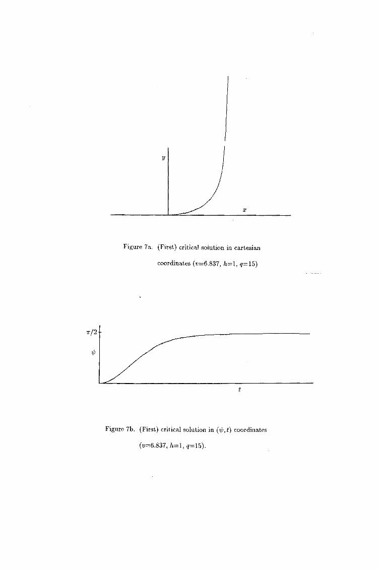
We now investigate the existence of the solution w(t, Ve), where Ve is such that we have the intuitively
most likely solution of (2.8), as sketched in fig. 7. In the next section we shall show that this solution
has minimal bending energy.
Two particular properties of the sought solution are
solution
(4.la) 0 < ,P(t, Ve) < 1f/2
(4.lb) 0 < ~(t,ve)
O<t<oo
O<t<oo
7
Page 11
In the original problem setting, we considered v as a parameter to be determined along with the
solution from an ODE formulation (via v = 0). Here we shall look for such values of v that the ODE
(2.6a) with (2.7a) has a solution with the properties {4.1) by fine tuning v. Inspired by (4.1), let us define
two sets of v-values giving rise to two families of solutions '¢ of (2.6a), (2.7a)
(4.2a) V1 = {v > 0!(3tl < oo) (~(t1, v) = 0) A ('rfi(t, v) < 1r/2, 0 < t < tl)}
(4.2b)
The sets V1 and V2 are constructed such that either ( 4.1a) or ( 4.1b) does not hold.
Property 4.3. (i) vl n v2 0, (ii) Vc E R.t \ (Vl u V2)
Proof. (i) Suppose v E V1 n V2, then we obviously have t2 = t1. Hence ,P(t2,v) 1rf2, ~(t2,v) = 0.
From (2.6a) this implies that ;fo(t2, v) = h. If h = 0 then all derivatives of'¢ vanish, so '¢ is constant,
which is a contradiction. If h > 0, '¢must have a (local) minimum at t = t2, implying ~(t,v) < 0 for
t < t2. This, however, would only occur if v f/:. V2 , so the result follows by contradiction. ¢
(ii) Let v > 0, v f/:. V1 U V2, then
[Vt{(~ ::/ 0) V (3r < t with ,P(r) = 7r/2)}] A [Vt{('¢ ::/'lf'/2) V (3r < t with ~(r) = 0)})
However, both for t2 < t1 and t1 < t2 the requirements ~(it)= 0 and '¢(t2 ) = 7r/2 are mutually exclusive.
So ( 4.1) implies that '¢ converges as t -+ oo to, say, a constant c < 1r /2. Then ¢ -+ -(qt - v) cos c ::/ 0,
which give a contradiction. Hence '¢ -+ 1r /2 for t -+ oo if v is element of the complement of V1 U V2
(which, however, may be empty). ¢
We now finally arive at
Theorem 4.4. vl, v2, and the complement of vl u v2 are not empty; moreover sup('Vi) = Vc = inf(V2)·
Proof. (a) Let v be small (i.e. close to zero) and consider'¢ for t small. Then we may linearize (2.6a)
to obtain
'¢ = h'¢-qt+v.
8
Page 12
For this elementary equation it easily follows that for some small value oft, say t == t1, we have ,fr(t, v) == 0.
By choosing v small enough, '1/J can be kept as small as we like along [0, tt]; in any case small enough for
the linearization, and smaller than 1r /2, which thus yields a nonempty V1.
(b) To prove that V2 is nonempty, we look for large enough v. To start, we observe that fort-+ 0 such
that '1/J-+ 0 we have 'If;~ !vt2 • So for v-+ oo we have 'If;= 2/v at t = 2/v. Furthermore, using (2.9), we
have along 0 < t < vfq (as long as 'If;< 1r) t¢2 > 0, so¢> 0, and 'If; increases. Again using (2.9), we thus
obtain for 2/v < t < 3vf4q (and, of course, 'If; not close to 1r) t¢ 2 > (v- qt)sin 'If;> (v- qt)2/v > t· So
0 1 0
'If;> 1, 'If;= J0 f/Jdt > t, and therefore 'If; can be made arbitrarily large (at least larger than 1r/2) before
¢vanishes.
(c) From the foregoing and property 4.3 we conclude that sup(V1) = Ve = inf(V2) as follows. First,
we observe that if a v, exists, it is a single point: consider a solution 'If; = '1/Je + 4>, v Vc + £, in the
neighbourhood ofthe critical solution (4> and£ small). Then for large enough t, when 'f/;e-+ 1rj2, we have
if;= (qt- Ve)4>
with exponentially growing solutions. So near vc there can be no other critical v's.
Finally, only the existence of vc remains to be shown. For this, we consider a sequence of angles,
increasing to 1r /2. With each angle we select a corresponding solution 'lj;n of which ¢n vanishes for the
first time at this angle (at time t = t 1,n, say). So by definition, the corresponding sequence {vn} is a.
subset of Vi. Since ;p(tl,n) < 0 we have with (2.6a)
qt1 > V + h tg'f/;(tl,n)
so t1,n-+ oo, and we have thus constructed a sequence in V1 converging to Ve· <>
5. Further investigations of the equation (2.8)
It is interesting to note that we should expect a sequence of critical v values, of which Ve, considered
in the previous section is just the first member. Intuitively this follows immediately from the pendulum
analogy as mentioned in §3. Here we like to look for a more precise (though qualitative) characterization.
9
Page 13
Before we do that we remark that the existence of another such 'critical v' will complicate the numerical
problem, as sketced in §2, even more; for if we might zoom in on that wrong value, during some iterative
procedure (say due to a completely off-value initial estimate for v), we not only encounter the troubles
associated with so many close solutions, but also the fact that our solution is completely wrong, if it
converges at all.
Let us recall the energy density relation (2.9). We can characterise a solution ,P(t, v) by its energy
(5.1) , 11 1 111/J(I,v)
E1(v) = 0 2~2(r, v) dr = 2 0
~(r, v) d,P
In our problemsetting we are interested more particularly in the case l - oo and the question therefore
arises whether E00 (v) exists. This question is addressed in the following two properties.
Property 5.2. E00 (vc) is finite.
Proof. If t is sufficiently large, we have
h ,P(t, ve) = 1r/2- arctg---:::::. 1r/2- hfqt
qt- Ve
. . I . So ,P(t, vc) = hfqt2 + O(r3), i.e. [,P(t, vc)J2 = o(t-4 ). Hence t fo t/;2( r, vc)dr converges as 1- oo. <>
Property 5.3. If lim,_,.00 ,P(t, v) :f. 1rj2 then lim,_00 ,P(t, v) = 31r /2.
Moreover lirrll-.00 Ez(v) does not exist.
Proof. As we have seen in §3, 37r/2 is the only alternative attractor. So let ,P(t) = [31r/2+¢(t)] mod (27r),
then
{; = -qt sin 4> = -qtqi.
The latter equation is therefore approximately equal to the Airy equation (cf. ref.12) with appropriate
scaling of variable. So we can write
,P(t) = aAi( -tjqt) + {JBi( -tjqt),
for some a, {J E IR. Hence ,fo(t) = aAi + [JBi "" tt sin(tt), so that [J,(t)J2 = d· sin2 (fi). Since (with
t = rt)
10
Page 14
we see that forT-+ oo this integral and thus ET(v) (see 5.1)) diverges. <>
Theorem 5.4. Considered as a function of v, Eoo ( v) has a local minimum at v Ve.
Proof. (a) Denote by t1(v) the first time that ;j; = 0 (to become negative). Since iPe starts positive and
finally becomes negative, it follows that T = liiiltJ-vc t1(v) < oo, and limv-vc .,P(ib v) < 1rj2. Hence there
is a subset v-2 c v2 with
Let v E V2. Then by definition there is a time t2 where .,P = 1rj2. Here, ;j; = h > 0, so there is another
time t2 with t1 < t2 < t2, where ;j; = 0 to become positive. Now denote by ~(.,P,w) the moment (or
'speed') tP as a function of the angle, and consider along [0, 1r /2] four sectors:
I: [0, .,P(T, ve)] ( ~(T, ve) = 0, force becomes negative after t T for v = ve)
In I the 'force' ;fi is larger for the choice v than for ve. Hence with v the point .,P(T, vc) is reached
earlier and with a higher speed. In II this effect is reinforced as for the case Ve the motion is slowed down
in contrast to the case v. In III we have
qt( V) < qt( Ve),
so for any angle a EIII, h sin a ( qt( v) - v) cos a > h sin a - ( qt( Vc) - Ve) cos a. Hence, despite the 'force'
being negative, it is less negative for v than for Ve·
Finally, in IV the motion for v is accelerated again, in contrast to ve. Summarising we thus have
found: for any .,P E (0,1f/2) is ~(.,P,v) > ~(t/J,ve)· From (5.1) we deduce
111t/2. Eoo(ve) < -
2 4>(1/J,v) d.,P < lim E,(v).
0 1-+oo
(b) Let v E vl (see (4.1a)) be very close to Ve. At the backward swing the pendulum passes the point
.,P = 0 again, at time t = t3 , say. We have there ;fi(t3 , v) = -(qt3 - v) (which is of course < 0). Now let
the maximal 'force' ;j; at tP(t, vc) on [0, .,P(T, vc)] be m. Then it is possible by choosing tg large enough to
11
Page 15
make the 'force' ;fat 'f/;(</J,v) on [0,-'f/;(T,vc)] larger in absolute value than m (by choosing v sufficiently
close to v.,); on [-t/;(T, vc), -11"/2] the force for'¢ is definite negative. We conclude from this that for such
a choice of v the 'speed' ¢on [0, -?r/2] is larger in modulus than ¢('¢, ve) on [0, 11" /2], whence
11-r/2 . E00 (vc) < -
2 <P('¢, v) d'¢ < lim E,(v).
o 1-oo
From(*) and(**) we deduce that Eoo(ve) is a local minimum. <>
Remark. The proof for the case v < Vc (part (b)) of the preceding theorem can also be based on
employing the fact that for v sufficiently dose to Vc limt-oo 1/J( t, v) -+ -11" /2 and using this fact in
combination with Properties 5.2 and 5.3.
The question remains which of the solutions converging to 1rj2 is the best. Apart from the solution
'f/;(t,v.,) characterised by (4.1) we may expect e.g. another solution '¢(t,ve2) say with Ve2 > Vc =:Vet.
having a terminal value limt ..... 00 fjJ(t,vc2 ) = 511"/2; i.e. this solution is still monotonic, passes 11"/2 to
come at rest only after completing another cycle. Similarly there are Ve& to be expected such that
limt-oo 'f/;(t,Vei) 11"/2 + (i- 1)211", ~(t) > 0. Existence will not be considered here, but basically we
anticipate it to be similar as for the case of Vel· Also, for v < Vet we may conjecture a sequence of 'v-
values', such that after an initial interval~> 0, there is a point t(v) where ~(t(v)) = 0, 0 < 'f/;(t(v),v) <
1rj2, and~< 0 fort> t(v), limt-oo 'f/;(t,v)-+ -11"/2- 2k11". It is interesting to realise, however, that
whatever other critical value of v may exist, Vc = Vet is optimal in the sense of minimal energy, as is
shown in
Theorem 5.5. E00 (vc) is the global minimum.
Proof. Ve2 should apparently be larger than Vel' as follows from the construction of the set v2. If Vc2 E v-2
then it follows from part (a) of the proof of Theorem 5.4 that t J;12 ¢('¢, Vc2) df/J < Eoo( vc)·
If Vc2 E V2 \ V2 then it is simple to see that ¢( 'f/;, Ve2) > ¢( 1/J, Vel) like in the aforementioned proof and
r/2 · thus that again t f0 tfJ(t/J, Ve2) d'¢ < E00 (vci). <>
12
Page 16
Conclusion
In this paper we have considered how the theoretical shape of a pipe depended on the value of the
bottom reaction force V. The 'natural shape' for some critical value of v Vc for a long pipe was shown
to have minimal bending energy. However, there are values of v arbitrarily close to Vc, where this shape
is completely different. This then explains (at least partially) why the nonlinear boundary value problem
resulting from the pipe laying model is hard to solve without special techniques. A possible way out for
this last problem is to use appropriate continuation techniques (e.g. in the length). Further investigations
are currently under way.
References
1. D.A. Dixon, D.R. Rutledge, Stiffened Catenary Calculations in Pipeline Laying Problem. Journal
of Engineering for Industry lll! (1), 1969, pp. 153-160.
2. J.T. Powers, L.D. Finn, Stress Analysis of Offshore Pipelines During Installation, Offshore Technol
ogy Conference 1071, 1969.
3. J .R. Wilkins, Offshore Pipeline Stress Analysis, Offshore Technology Conference 1227, 1970.
4. G.C. Daley, Physical Interpretations of the Instabilities Encountered in the Deflection Equations of
the Unconstrained Pipeline, Offshore Technology Conference 1933, 1974.
5. P. Terndrup Pedersen, Equilibrium of Offshore Cables and Pipelines During Laying, International
Shipbuilding Progress, Vol.22, Dec. 1975, pp.399-408.
6. G. Maier, Optimization of Stinger Geometry for Deepsea Pipelaying, Journal Energy Resources Tech.
104. pp.294-301.
7. I. Konuk, Higher Order Approximations in Stress Analysis of Submarine Pipelines, ASME paper
80-PET-72, 1980.
8. S.W. Rienstra, Analytical Approximations For Offshore Pipelaying Problems, Proceedings of the
First International Conference on Industrial and Applied Mathematics ICIAM 87, Paris 1987, Con
tributions from the Netherlands. (WI Tract 36, ed. by A.H.P. van der Burgh and R.M.M. Mattheij,
1987).
13
Page 17
9. M.J. Brown, L. Elliott, Pipelaying From a Barge, Mathematical Engineering For Industry l (1),
1987, pp.33-46.
10. R. Frisch-Fay, Flexible Bars, Butterworths, London 1962.
11. L.D. Landau, E.M. Lifshitz, Theory of Elasticity, Pergamon, Oxford, 1970.
12. M. Abramowitz, LA. Stegun (eds.), Handbook of Mathematical Functions, National Bureau ofStan-
dards 1964.
R.M.M. Mattheij, Faculteit Wiskunde en Informatica, Technische Universiteit Eindhoven, Postbus 513,
5600 MB Eindhoven, The Netherlands.
S.W. Rienstra, Wiskundige Dienstverlening, Faculteit Wiskunde en Natuurwetenschappen, Katholieke
Universiteit, Toernooiveld, 6525 ED Nijmegen, The Netherlands.
--I welding ramp)
=+
Figure 1. Sketch of the pipelay problem
y Vs + Qds
X
Figure 2 Equilibrium of pipe element
Page 18
-0.5
-0.5
y
1.
0. 0.5
Figure 3a. v=6.61, h=l, q=l5
y
1.
o. 0:5
Figure 3c. v=6.98, h=l, q=l5
1.
1. X
y
1.
0.5 0. 0.5 1. X
Figure 3b. v=6.74, h=l, q=15
y
1.
-0.5 0. 1. 1.5 X
Figure 3d. v=35.74, h=l, q=15
Page 19
end of oscillation interval
1b(O) = 0 J>(o) = o
Figure 4a. Kirchhoff's pendulum analogy for q=O.
Constant gravity field ( -h, v)
Figure 5a. Pendulum analogy (radial coordinate grows
linearly in time) for v=6, h=l, q=15.
1/;(0) = 0 J>(o) = o
h------... __ _
Figure 4b. Generalized pendulum analogy.
Time dependent gravity field ( -h, v- qt).
¢(t)
Figure 5b. v=35.63, h=l, q=l5
Page 20
y
y
1.
L
-1. 0. X 1.
-1. 0. 1. 2. X
Figure 6b. v=69, h=l, q=l5
Figure 6a. v::::6.837, h::::l, q::::l5 0. 2.
y
y
1. 0. X I.
Figure 6c. v::::lOO, h::::l, q=l5 Figure 6d. h=l, q=15
Page 21
y
X
Figure 7 a. (First) critical solution in cartesian
coordinates (v=6.837, h=l, q=15)
t
Figure 7b. (First) critical solution in ('1/J,t) coordinates
(v=6.837, h=l, q=15).