JOURNAL OF ECONOMIC THEORY 4, 200-223 (1972)

On Capital Overaccumulation in the Aggregative,

Neoclassical Model of Economic Growth:

A Complete Characterization

DAVID CASS *

Graduate School of’ Industrial Administration, Carnegie-Mellon University, Pittsburgh, Pennsylvania 15213

Received March 29, 1971

I. INTRODUCTION

Consider the following idealized description of an economy’s behavior over time: In each period the labor force works with several different types of capital stocks to produce several different types of output. These last are then used either to satisfy the needs and wants of the first (consumption) or to replace and augment the second (investment). Both production and the allocation of output between consumption and investment are carried out efficiently; that is, in any given period no output could be increased without another being decreased, and at the end of any span of periods no capital stock could be increased without another or some intermediate consumption being decreased. Such an evolution starts from a given profile of capital stocks and continues indefinitely.

Now ask the question: Is this seemingly exemplary economy actually providing as much consumption as it’s capable of? A moment’s reflection should convince one that the correct answer is that it all depends on whether, in some sense, too much investment takes place. In particular, just consider the polar situation where in every period all output is invested (and consequently, the economy provides no consumption whatsover!).

* Ned Phelps deserves credit (or perhaps blame) for stimulating my original interest in this problem, while without fruitful collaboration with Manny Yaari, upon which I draw very heavily at points, I would have long ago abandoned the attempt to solve it to my own satisfaction. Support from the following three sources is very gratefully acknowledged: A National Science Foundation grant to the Cowlea Foundation for Research in Economics at Yale University, the Graduate School of Industrial Ad- ministration at Carnegie-Mellon University, and a John Simon Guggenheim Memorial Foundation Fellowship for a year’s leave at the University of Tokyo.

200 @ 1972 by Academic Press, Inc.

ON CAPITAL OVERACCUMULATION 201

On Capital Overaccuniulation

The purpose of this paper is to explore, in a systematic way, the circum- stances in which it is possible to say definitely that such a phenomenon, excessive investment or capital overaccumulation, is or is not occurring. That is, I attempt to answer the question: What observable characteristic of a growth path signals capital overaccumulation (or its absence) ? In order to focus on this question, I consider a model which abstracts from problems of efficiency of the sort mentioned in the opening paragraph (say, of short-run eficiency) and permits only the problem of over- accumulation (say, of long-run eficiency), the now standard aggregative, neoclassical model of economic growth. My principal reasons for this drastic simplification are first, a strong belief that economists had best understand long-run efficiency (or simply, when there is no confusion possible, efficiency) in its barest possible context before going on to tackle more complex models (with, to some extent, superfluous complications), and second, a naive hope that the results gleaned here will point the way for more general ones. I will come back at the end to consider the degree to which this hope appears justified.

It also turns out that, even in this very simple model, answering the question posed becomes quite involved. The fundamental result, initially presented in Section IV, is a complete characterization of inefficient growth paths in terms of the asymptotic behavior of the economy’s net interest rate. Roughly speaking, the criterion is that a growth path is inefficient if and only if the terms of trade from the present to the future worsen at a sufficiently rapid rate as the future recedes into the distance. But to elab- orate its proof, to say nothing about motivating and interpreting it, requires fairly lengthy and intricate analysis, finally detailed in Section V.

However, the true test of such a result is not whether it’s easily proved or understood, but whether it really enables one to determine-given just a description of production technology and saving-investment behavior- the efficiency or inefficiency of a wide range of growth paths. This criterion passes that test with high marks, at least in terms of the examples I (and Yaari) came to regard as benchmarks. Several of these are elaborated, to support my claim, and thereby provide additional motivation for the criterion before proving it in Section IV. It would be interesting to carry the test further with growth paths whose efficiency others think useful or instructive to determine.

Finally, let me comment a bit on the relation of this paper to the literature: The bulk of the published work on the problem of long-run efficiency has concentrated on providing a price interpretation for efficient growth paths, starting from the lead of Malinvaud’s beautiful, seminal

202 CASS

paper [4, 51. Especially notable contributions to this development are Radner’s piece generalizing the concept of efficiency prices [9] and Yaari’s work with myself and Peleg generalizing the interpretation of efficiency prices [2, 61. While this approach is an intellectually appealing way of attacking the problem-primarily because it’s in a long-standing theoretical tradition-unfortunately, the results derived from it have little to offer by way of answering the central question posed above. That is, knowing that an efficient growth path is in some sense maximal with respect to some sort of valuation just doesn’t enable a concrete judgment about the efficiency of any particular growth path. Thus my own preference is for a more direct attack.

In that direction, there have been only a few published papers-to my knowledge all dealing with the aggregative, neoclassical model analyzed here-attempting to establish immediately applicable criteria. Most striking is Phelp’s result that having the capital stock asymptotically strictly above the golden rule path is inefficient [7], later extended to a wider class of comparison paths [8]. Indeed, as I have already noted, Phelp’s work aroused my own interest, and this paper might very well be thought of as an attempt to complete the investigation he began.

II. THE MODEL: ASSUMPTIONS AND DEFINITIONS

Starting from a given initial capital stock A, (2 b), the economy evolves over periods t = 0, l,... according to the basic growth equation

k t+l =fW - Ct with kt 3 K, ct 3 0, (1)

where kt is the capital stock at the beginning of period t, f is the gross output function’ for period t, ct is consumption during period t and K >0 provides a lower bound on gross output2. f is assumed to be strictly

1 In the sense that it includes whatever capital is not used up in production during period t. f(k) - k therefore corresponds to the more standard notion of net output (consumption plus gross investment less depreciation). Also see the interpretation of the model sketched two paragraphs below.

2 Below which the economy would effectively disappear, say, because of the ensuing breakdown of the economic system. The assumption B > 0 is only necessary for the analysis presented to encompass the possibility f’(0) = co, as is the case, for example, when f is essentially the CobbDouglas production function

f(k) = Ak= + Bk with A>O;O<ol,B< 1.

ON CAPITAL OVERACCUMULATION 203

increasing, strictly concave (withf” < 0) and twice continuously differen- tiable for k > 0, and to satisfy the endpoint conditions

f(O) = 0 and 0 <f’(m) < 1 <f’(k) < co.

From these assumptions aboutfit follows that there are unique capital stocks 0 < R* < 7 < co defined by

f’(k*) = 1 and f(z) = 2. (2)

R* is thus the golden rule capital stock (i.e., the capital stock for which consumption is maximum among steady states), 2 the maximum main- tainable capital stock (i.e., the highest capital stock the economy can maintain in the long-run even if all output were invested). The existence of the latter means that without any loss of generality we can also assume A,, < 2 which entails k, < 2 for t = 0, l,... . Then, from the first three assumptions about f it follows that there are bounds 0 < m < M < co (in particular, m = min,,,,E --f”(k), A4 = maxf,,Gk --f”(k) will do) on the rate at which the net interest rate in this economy N f’ [more precisely, a + bf’ with b > 0; see below] changes with capital intensity k

for m(kl - k”) ,( f’(kO) -f’(kl) < M(kl - k”)

& < k” < k1 < 2. (3)

Condition (3) may be rewritten more conveniently as the following pair of inequalities

f’(k) + me < f’(k - 4 <f’(k) + ME for K<k--<k<2,

(4) which in turn imply the additional pair of inequalities

[ f’(k) + 7-j E <f(k) - f(k - 4 < [f’(k) + F] E for

K<k--E,<k<2,3

results I will refer to repeatedly in the seque14. (5)

3 In fact, the left-hand-but not the right-hand-inequalities in (4) and (5) are equivalent.

4 Conditions (4) and (5) (which are essentially strong statements about the concavity and regularity of fl are basic to most of the proofs in the paper. Morever, some such restriction on intertemporal production possibilities is required for my results as well, a point I shall return to at some length in Sections V and VI. Notice, however, that condition (4) could, to some extent, accommodate arbitrary technical progress (besides that of the usual Harrod-neutral sort).

204 CASS

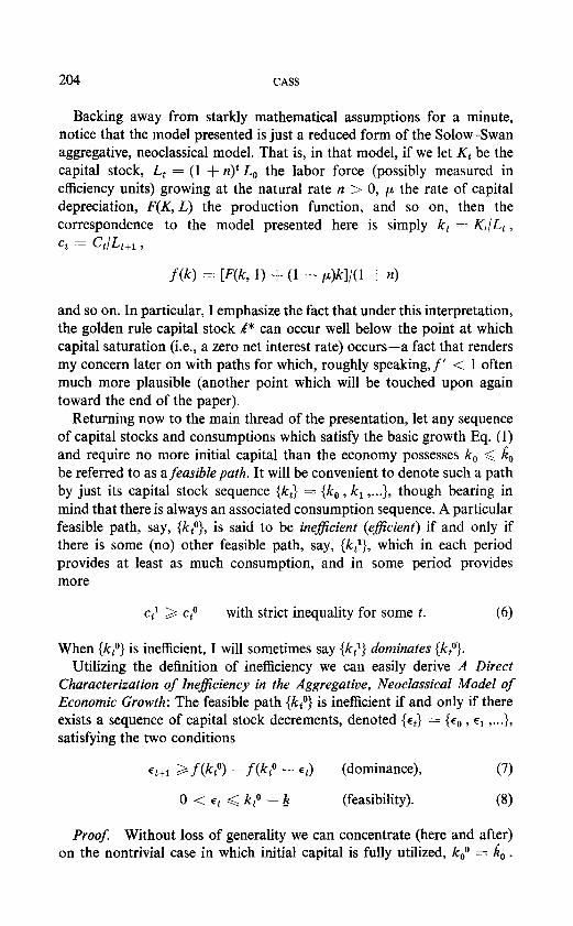
Backing away from starkly mathematical assumptions for a minute, notice that the model presented is just a reduced form of the Solow-Swan aggregative, neoclassical model. That is, in that model, if we let Kt be the capital stock, Lt = (1 + n)” L, the labor force (possibly measured in efficiency units) growing at the natural rate rr > 0, p the rate of capital depreciation, F(K, L) the production function, and so on, then the correspondence to the model presented here is simply kt z= K,/& , Ct = GL,l ,

f(k) = VW 1) + (1 - /4Wl + 4

and so on. In particular, 1 emphasize the fact that under this interpretation, the golden rule capital stock A* can occur well below the point at which capital saturation (i.e., a zero net interest rate) occurs-a fact that renders my concern later on with paths for which, roughly speaking, f’ < 1 often much more plausible (another point which will be touched upon again toward the end of the paper).

Returning now to the main thread of the presentation, let any sequence of capital stocks and consumptions which satisfy the basic growth Eq. (1) and require no more initial capital than the economy possesses k, ,< & be referred to as a feasible path. It will be convenient to denote such a path by just its capital stock sequence {k,} = {k, , k, ,...}, though bearing in mind that there is always an associated consumption sequence. A particular feasible path, say, {k,O}, is said to be ineficient (eficient) if and only if there is some (no) other feasible path, say, {k,l}, which in each period provides at least as much consumption, and in some period provides more

ctl b $0 with strict inequality for some t. (6)

When {k,O} is inefficient, I will sometimes say {k,l) dominates {k,O}. Utilizing the definition of inefficiency we can easily derive A Direct

Characterization of Ineficiency in the Aggregative, Neoclassical Model of Economic Growth: The feasible path {k,O} is inefficient if and only if there exists a sequence of capital stock decrements, denoted {et> = {co, c1 ,...}, satisfying the two conditions

et+1 2f(kt”) -fW - 4 (dominance), (7)

O<q<k:-& (feasibility). (8)

Pro05 Without loss of generality we can concentrate (here and after) on the nontrivial case in which initial capital is fully utilized, k,O = x0 .

ON CAPITAL OVERACCUMULATION 205

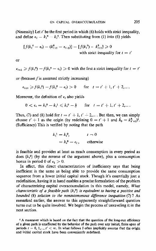
(Necessity) Let t’ be the first period in which (6) holds with strict inequality, and define et = kto - ktl. Then substituting from (1) into (6) yields

Lf(k,o - 4 - (@+1 - %,I>1 - Lf@,o) - e+11 3 0 with strict inequality for t = t’

or

E~+~ > f&o) --f(k,o - l t) 3 0 with the first a strict inequality for t = t’

or (because f is assumed strictly increasing)

Et+1 >.mtO) --f(bO - 4 > 0 for t = t’ + 1, t’ + 2,... .

Moreover, the definition of l t also yields

0 < l t = kto - k,l < k,O - K for t = t’ + 1, t’ + 2,... .

Thus, (7) and (8) hold for t = t’ + 1, t’ + 2,... . But then, we can simply choose t’ + 1 as the origin (by redefining 0 = t’ + 1 and A0 = k$+1)5. (Sufficiency) This is verified by noting that the path

k$ = kto, t=O

= kt” - Et , otherwise

is feasible and provides at least as much consumption in every period as does {k,O) (by the reverse of the argument above), plus a consumption bonus in period 0 of e1 > 0.

In effect, this direct characterization of inefficiency says that being inefficient is the same as being able to provide the same consumption sequence from a lower initial capital stock. Though it’s essentially just a redefinition, having it in hand enables a precise formulation of the problem of characterizing capital overaccumulation in this model, namely, What characteristic of a feasible path {kto} is equivalent to having a positive and bounded (8) solution to the nonautonomous difference inequation (7) ? As remarked earlier, the answer to this apparently straightforward question turns out to be quite involved. We begin the process of unraveling it in the next section.

6 A maneuver which is based on the fact that the question of the long-run efficiency of a given path is unaffected by the behavior of the path over any initial, finite span of periods t = 0, I,..., f’ < co. In what follows I often implicitly assume that the origin and initial capital stock have been conveniently redefined.

206 CASS

III. A PARTIAL CHARACTERIZATION: INCREASINGLY UNFAVORABLE TERMS OF TRADE FROM THE PRESENT TO THE FUTURE

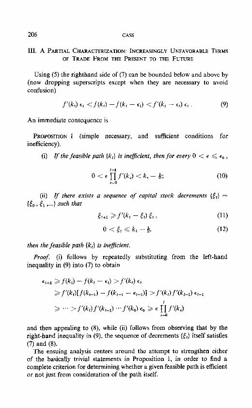
Using (5) the righthand side of (7) can be bounded below and above by (now dropping superscripts except when they are necessary to avoid confusion)

f’(kt) Et <f(k) -mt - 4 < f’(kt - 4 Et * (9)

An immediate consequence is

PROPOSITION 1 (simple necessary, and sufficient conditions for inefficiency).

(i) lf the feasible path (k,) is ineficient, then fur every 0 < E < Ed ,

t-1

0 < E n f’(k,) < k, - k; CT=0

(10)

(ii) If there exists a sequence of capital stock decrements {tt} = (to, f1 ,...I such that

St+1 2 f’(kt - 43 5t , (11)

0 < tt G kt - k, (12)

then thejbasible path (k,) is ineficient.

Proof. (i) follows by repeatedly substituting from the left-hand inequality in (9) into (7) to obtain

et+1 > f(h) - f& - 4 > f’(kt> et

3 f’(k,)[f(k,-,) - f(k,-, - dl > f’Vdf’&-J et-1

>, -*a >f’(kt)f’(kd .-*f’(ko) l 0 3 E n f’(ks> s=O

and then appealing to (8), while (ii) follows from observing that by the right-hand inequality in (9), the sequence of decrements {Et) itself satisfies (7) and (8).

The ensuing analysis centers around the attempt to strengthen either of the basically trivial statements in Proposition 1, in order to find a complete criterion for determining whether a given feasible path is efficient or not just from consideration of the path itself.

ON CAPITAL OVERACCUMULATION 207

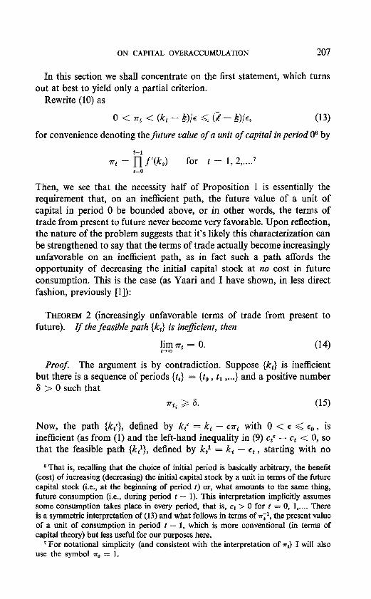
In this section we shall concentrate on the first statement, which turns out at best to yield only a partial criterion.

Rewrite (10) as

0 < 7rt < (k, - K)/E d (2 - g/e, (13)

for convenience denoting the future value of a unit of capital in period O6 by

t-1

=t = j-J f’(ks> for t = 1, 2,....’ s=o

Then, we see that the necessity half of Proposition 1 is essentially the requirement that, on an inefficient path, the future value of a unit of capital in period 0 be bounded above, or in other words, the terms of trade from present to future never become very favorable. Upon reflection, the nature of the problem suggests that it’s likely this characterization can be strengthened to say that the terms of trade actually become increasingly unfavorable on an inefficient path, as in fact such a path affords the opportunity of decreasing the initial capital stock at 120 cost in future consumption. This is the case (as Yaari and I have shown, in less direct fashion, previously [l]):

THEOREM 2 (increasingly unfavorable terms of trade from present to future). If the feasible path {k,) is ineficient, then

pi ?rt = 0. (14)

Proof. The argument is by contradiction. Suppose {k,} is inefficient but there is a sequence of periods {tJ = (to , t, ,...} and a positive number 8 > 0 such that

rrti b 6. (15)

Now, the path {ktf}, defined by kt’ = kt - l rt with 0 < E < eo, is inefficient (as from (1) and the left-hand inequality in (9) ctC - ct < 0, so that the feasible path {k,l}, defined by ktl = kt - Et, starting with no

B That is, recalling that the choice of initial period is basically arbitrary, the benefit (cost) of increasing (decreasing) the initial capital stock by a unit in terms of the future capital stock (i.e., at the beginning of period t) or, what amounts to the same thing, future consumption (i.e., during period 1 - 1). This interpretation implicitly assumes some consumption takes place in every period, that is, ct > 0 for t = 0, l,.... There is a symmetric interpretation of (13) and what follows in terms of n;‘, the present value of a unit of consumption in period t - 1, which is more conventional (in terms of capital theory) but less useful for our purposes here.

’ For notational simplicity (and consistent with the interpretation of ~3 I will also use the symbol r,, = 1.

208 CASS

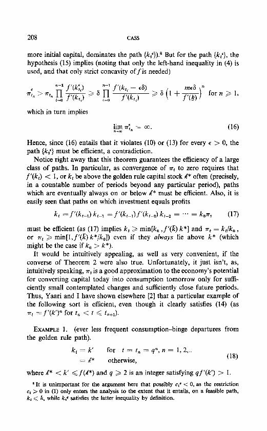
more initial capital, dominates the path {k,}).” But for the path {k;}, the hypothesis (15) implies (noting that only the left-hand inequality in (4) is used, and that only strict concavity off is needed)

,,--l f ‘(k;J n-1 f’(kdi - ~8)

“k > ntn sg f’(kti) ’ ’ E f ‘@ii) 3 6 (1 + G)” for Iz > 1,

which in turn implies

‘n’j 77;” = co. (16)

Hence, since (16) entails that it violates (10) or (13) for every E > 0, the path {k,‘} must be efficient, a contradiction.

Notice right away that this theorem guarantees the efficiency of a large class of paths. In particular, as convergence of 7rt to zero requires that f ‘(kJ --c 1, or k, be above the golden rule capital stock A* often (precisely, in a countable number of periods beyond any particular period), paths which are eventually always on or below A* must be efficient. Also, it is easily seen that paths on which investment equals profits

k, = f ‘(k& k,-, = f’(k,-,)f’(k,-,) k,-, = ... = kg-, (17)

must be efficient (as (17) implies k, > min[k, , f ‘(E) k*] and 7rt = kJk, , or 7~~ 3 min[l,f’(k) k*/k,]) even if they always lie above k* (which might be the case if k, > k*).

It would be intuitively appealing, as well as very convenient, if the converse of Theorem 2 were also true. Unfortunately, it just isn’t, as, intuitively speaking, 7rt is a good approximation to the economy’s potential for converting capital today into consumption tomorrow only for suffi- ciently small contemplated changes and sufficiently close future periods. Thus, Yaari and I have shown elsewhere [2] that a particular example of the following sort is efficient, even though it clearly satisfies (14) (as rt = f’(k’)” for t, < t < t,,,).

EXAMPLE 1. (ever less frequent consumption-binge departures from the golden rule path).

kt = k’ for t = t, = q”, n = 1, 2,.. = R* otherwise, (18)

where A* < k’ < f(n*) and q >, 2 is an integer satisfying qf’(k’) > 1.

* It is unimportant for the argument here that possibly cte < 0, as the restriction ct > 0 in (1) only enters the analysis to the extent that it entails, on a feasible path, kt < R, while kf satisfies the latter inequality by definition.

ON CAPITAL OVERACCUMULATION 209

To illustrate the applicability of the result of the next section, we will return to this example there.

The upshot of this section is that the first statement in Proposition 1 really can’t be strengthened to yield a complete criterion. The partial criterion (14) is quite useful, though, because it reduces the search for inefficient paths from looking at the class of all feasible paths, to looking at just those feasible paths on which future value converges to zero. Furthermore, Theorem 2 and Example 1 strongly suggest that what is needed to complete that search is some condition concerning the rate at which the terms of trade from the present to the future worsen. What about strengthening the second statement in Proposition 1 to provide such a condition? The balance of the paper is devoted to exploring this possibility.

IV. A COMPLETECHARACTERIZATION: 1 .STATEMENT,~NTERPRETATIONAND EXAMPLES

At first glance, the prospect of strengthening the second statement in Proposition 1 doesn’t seem very promising; in particular, the obvious conjecture-the converse of that statement -seems not very likely, and even if true, seems not very useful. But here is where the strong assumptions about concavity of the gross output function and regularity of the net interest rate (4) come into prominence: By a fairly indirect chain of reasoning-partly elaborated in the next section-the lead provided by my attempt to strengthen the sufficiency half of Proposition 1 was coaxed to yield the following strikingly simple criterion, which also appears as fundamental as the structure of the problem allows.

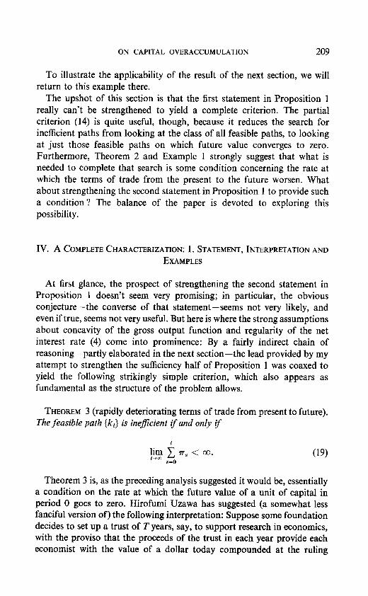
THEOREM 3 (rapidly deteriorating terms of trade from present to future). The feasible path (k,) is inefjcient if and only if

Theorem 3 is, as the preceding analysis suggested it would be, essentially a condition on the rate at which the future value of a unit of capital in period 0 goes to zero. Hirofumi Uzawa has suggested (a somewhat less fanciful version of) the following interpretation: Suppose some foundation decides to set up a trust of T years, say, to support research in economics, with the proviso that the proceeds of the trust in each year provide each economist with the value of a dollar today compounded at the ruling

210 CASS

market rate of interest. Then, if (i) the number of economists grows roughly at the same rate as the number of ordinary laborers, but none- theless (ii) their combined wisdom won’t prevent the economy from pursuing an excessive growth policy, and moreover (iii) the foundation is sufficiently wealthy and far-sighted (so the term of the trust is large), the cost of establishing the trust will exceed its benefits (both measured in current dollars).

The real point of this allegory is that, being a statement about speed of convergence, the criterion (19) doesn’t have a simple, neat economic interpretation; rather, its virtue is its relatively straightforward application to a wide variety of cases. Before demonstrating that claim with several examples, however, let me mention another way (i.e., besides that already contained in Theorem 2) of partly restating (I 9) which perhaps sheds some additional light on its meaning.

Knowing that the question of efficiency basically depends on the asymptotic behavior of nt , one possibility that suggests itself is to consider instead the asymptotic behavior of a related concept, the economy’s average rate of interest

I + Rt = (nt)'lt.

It can be shown directly, but follows more simply by applying well-known results from the theory of infinite series to Theorem 3, that (i) if for some negative number R < 0 there is a period T < co such that ever after the average rate of interest Rt is below R,

Rt<R<O for t 3 T,

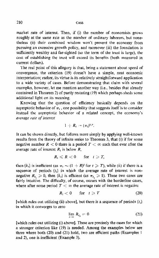
then {k,] is inefficient (as rrt - (1 + R)t for t > T), while (ii) if there is a sequence of periods {ti} in which the average rate of interest is non- negative Rti 3 0, then (k,} is efficient (as rti 3 1). These two cases are fairly intuitive. The difficulty, of course, occurs with the borderline cases, where after some period T < cc the average rate of interest is negative

R -0 t--. for t > T (20)

[which rules out utilizing (ii) above], but there is a sequence of periods {ti> in which it converges to zero

','% R,, = 0 + (21)

[which rules out utilizing (i) above]. These are precisely the cases for which a stronger criterion like (19) is needed. Among the examples below are three where both (20) and (21) hold, two are efficient paths (Examples 1 and 2), one is inefficient (Example 3).

ON CAPITAL OVERACCUMULATION 211

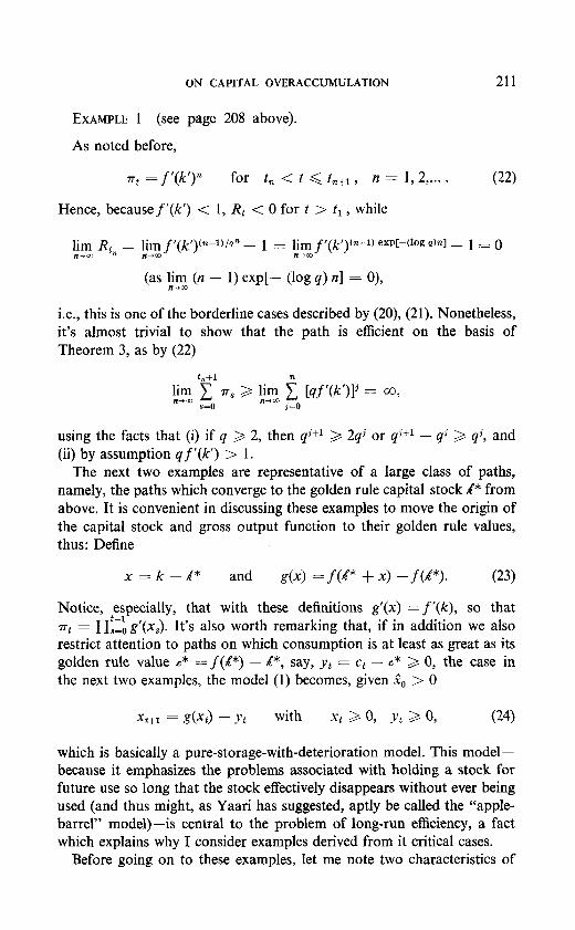
EXAMPLE 1 (see page 208 above).

As noted before,

%-t = f’(k’)” for t, < t < t,+l , n = 1, 2 ,... .

Hence, becausef’(k’) < 1, Rt < 0 for t > t1 , while

;i Rtn = l&j-‘(k’)Wqn - 1 = ;if’(k’)(“-1) exP[-(h3 e)nl - 1 = 0

(as $E (n - 1) exp[- (log q) n] = 0),

i.e., this is one of the borderline cases described by (20), (21). Nonetheless, it’s almost trivial to show that the path is efficient on the basis of Theorem 3, as by (22)

using the facts that (i) if q > 2, then qj+l > 2qi or qj+l - qi 2 qj, and (ii) by assumption qf’(k’) > 1.

The next two examples are representative of a large class of paths, namely, the paths which converge to the golden rule capital stock A* from above. It is convenient in discussing these examples to move the origin of the capital stock and gross output function to their golden rule values, thus: Define

x=k-lR” and g(x) = f (n* + x) - f(L”>. (23)

Notice, especially, that with these definitions g’(x) = f’(k), so that z-t = n”,r’, g’(xJ. It’s also worth remarking that, if in addition we also restrict attention to paths on which consumption is at least as great as its golden rule value C* =f(n*) - R*, say, yt = ct - C* > 0, the case in the next two examples, the model (1) becomes, given So > 0

xt+1 = g(xt) - Yt with Xt > 0, Yt >, 0, (24)

which is basically a pure-storage-with-deterioration model. This model- because it emphasizes the problems associated with holding a stock for future use so long that the stock effectively disappears without ever being used (and thus might, as Yaari has suggested, aptly be called the “apple- barrel” model)-is central to the problem of long-run efficiency, a fact which explains why I consider examples derived from it critical cases.

Before going on to these examples, let me note two characteristics of

212 CASS

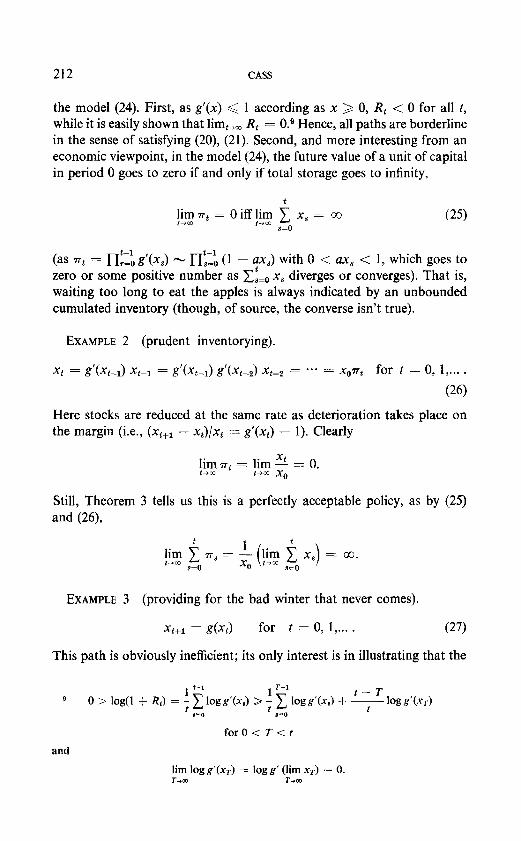
the model (24). First, as g’(x) < 1 according as x 3 0, R, < 0 for all I, while it is easily shown that lim,,, Rt = O.s Hence, all paths are borderline in the sense of satisfying (20), (21). Second, and more interesting from an economic viewpoint, in the model (24), the future value of a unit of capital in period 0 goes to zero if and only if total storage goes to infinity,

(2%

(as nt = JJ”,r’, g’(x,) - n”,r’, (1 - ax, WI h 0 < ax, < 1, which goes to ) ‘t zero or some positive number as xi=, x, diverges or converges). That is, waiting too long to eat the apples is always indicated by an unbounded cumulated inventory (though, of source, the converse isn’t true).

EXAMPLE 2 (prudent inventorying).

xt = g’(xt-l) x~-~ = g’(x,-,) g/(x,-,) xtmz = -a* = xo5-rt for t = 0, l,... .

(26)

Here stocks are reduced at the same rate as deterioration takes place on the margin (i.e., (xtfl - xt)/xt = g’(xt) - 1). Clearly

L% 7rt = pit 2 = 0.

Still, Theorem 3 tells us this is a perfectly acceptable policy, as by (25) and (26),

EXAMPLE 3 (providing for the bad winter that never comes).

-%fl = ‘et) for t = 0, I,... . (27)

This path is obviously inefficient; its only interest is in illustrating that the

9 0 > loid + R3 = ; slog&*) > ; Tflogs~(xs) + t-T

- log g’(.ur) t F-0 F-0

for 0 < T < t

and

lim log&h) = logg’ (lim xT) = 0. r+m T-K0

ON CAPITAL OVERACCUMULATION 213

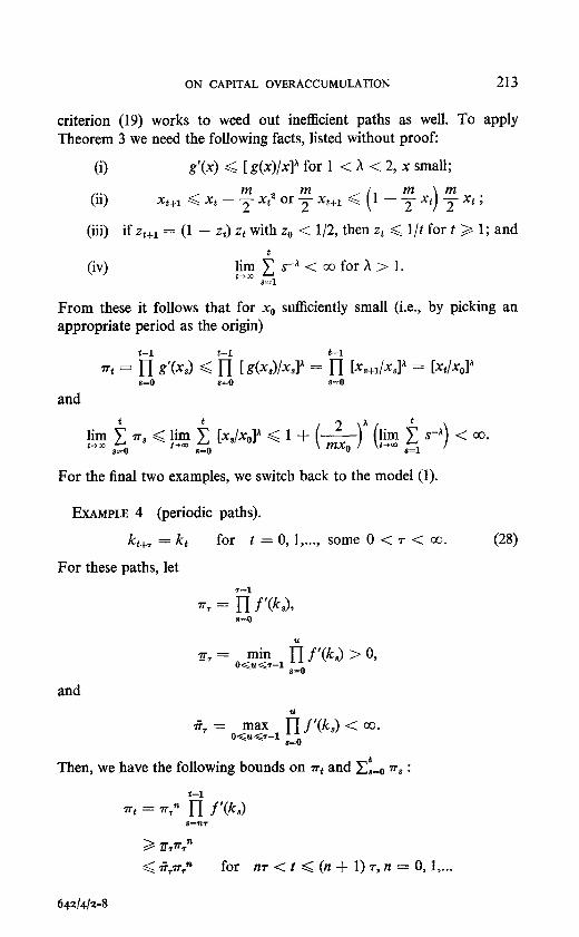
criterion (19) works to weed out inefficient paths as well. To apply Theorem 3 we need the following facts, listed without proof:

(9 g’(x) < [ g(x)/xlA for 1 < X < 2, x small;

(ii) xtfl < xt - 3 xt2 or 7 xt+l < ( 1 - T xt 1 7 xt ;

(iii) if zt+l = (1 - zt) zt with z,, < l/2, then zt < l/t for t > 1; and

(iv> $I~I i+<coforh>l. .9=1

From these it follows that for x,, sufficiently small (i.e., by picking an appropriate period as the origin)

t-1 t-1 t-1

=t = lJ gw < 5 [&Jl~,la = I-J [%+,/&I” = bt/%J”

and

For the final two examples, we switch back to the model (1).

EXAMPLE 4 (periodic paths).

k - kt t-%-r - for t = 0, I,..., some 0 < 7 < w. (28)

For these paths, let r-1

~7 = n f'(kJ, S==O

and

Then, we have the following bounds on rt and C”,=, rr8 :

t-1

64214/2-8

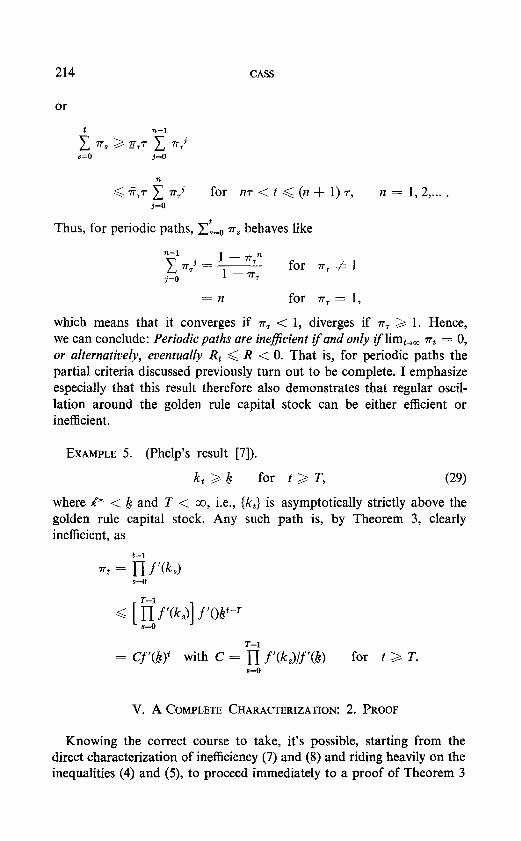
214 CASS

or

for ~7 < t < (n + 1) 7, n = 1, 2,... .

Thus, for periodic paths, C”,=, n, behaves like

for ?T, f 1

n for 7~~=1,

which means that it converges if rr7 < 1, diverges if n, 3 1. Hence, we can conclude: Periodic paths are ineficient ifand only zjlim,,, nt = 0, or alternatively, eventually R, < R < 0. That is, for periodic paths the partial criteria discussed previously turn out to be complete. I emphasize especially that this result therefore also demonstrates that regular oscil- lation around the golden rule capital stock can be either efficient or inefficient.

EXAMPLE 5. (Phelp’s result [7]).

kt 3 k for t 3 T, (2%

where R* < K and T < co, i.e., {k,} is asymptotically strictly above the golden rule capital stock. Any such path is, by Theorem 3, clearly inefficient, as

t-1

rt = I-I f’(kJ

T-l

= C”(K)t with C = n f’(k,)lf’@) for t > T. .S=O

V. A COMPLETE CHARACTERIZATION: 2. PROOF

Knowing the correct course to take, it’s possible, starting from the direct characterization of inefficiency (7) and (8) and riding heavily on the inequalities (4) and (5), to proceed immediately to a proof of Theorem 3

ON CAPITAL OVERACCUMULATION 215

(which starts with Lemma 2 below). More instructive, however, is to begin instead along the course I originally took, both because there’s an additional characterization of inefficiency to be gained-the converse of the second statement in Proposition 1, of some interest in its own right- and because in gaining that characterization we shall uncover a very close connection between it and Theorem 3.

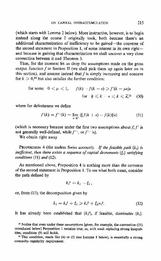
Thus, for the moment let us drop the assumptions made on the gross output function fin Section II (we shall pick them up again later on in this section), and assume instead that f is simply increasing and concave for k 3 O,l” but also satisfies the further condition:

for some 0 < p < 1, f(k) - f(k - ~1 3 f’(k - p+

for 4 < k - E < k < ,Z,ll (30)

where for definiteness we define

f’(k) = f’-(k) = ~${[f(k + 4 - fWli4 (31)

(which is necessary because under the first two assumptions about f, f’ is not generally well-defined, while f I-, orf’f is).

We obtain right away

PROPOSITION 4 (the useless Swiss account). If the feasible path {k,} is ineficient, then there exists a sequence of capital decrements (43 satisfying conditions (11) and (12).

As mentioned above, Proposition 4 is nothing more than the converse of the second statement in Proposition 1. To see what both mean, consider the path defined by

or, from (1 I), the decomposition given by

(32)

It has already been established that (k,‘}, if feasible, dominates {k,).

lo Notice that even under these assumptions [given, for example, the convention (31) introduced below] proposition 1 remains true, as, with weak replacing strong inequal- ities, condition (9) still holds.

I1 This condition, much like (4) or (5) ( see Lemma 1 below), is essentially a strong concavity-regularity requirement.

216 CASS

Hence, Proposition 4 together with the last half of Proposition 1 simply states that an inefficient path, and only an inefficient path, can be broken up into two parts, one productive-k tC, the capital stock required to maintain itself and provide at least the same consumption-the other unproductive -ct , a bank account, returning at least the same as the productive sector, but never being drawn upon. That is, in effect, the economy has a useless Swiss account.

Proof. Since {k,} is assumed inefficient, there exists a sequence of capital decrements {et} satisfying the inefficiency conditions (7) and (8). This implies, given the property (30), that

et+1 2 f(k,) -f&t - 4 3 f’(k, - pet) Et

or

with

0 < pet < et d kt - K.

Hence, tt = ~CLE~ satisfies conditions (11) and (12). Continuing on this course, the question now arises. When does (30)

hold ? That is, what properties off, in addition to monotonicity and concavity, would imply (or are implied by) condition (30) ? This leads to

LEMMA 1 (a property of sufficiently regular and concave functions of a real variable). Zf f satisfies condition (4), then it also satisfies condition (30).12

Thus, in particular, Proposition 4 remains valid under our original assumptions onf. I haven’t pursued the question of whether condition (30) also holds under the slightly weaker assumptions of strict concavity and

la I am now reverting to the assumption that f’ exists (i.e.,f’- = f ‘f = f ‘). Suppose instead that condition (4) were interpreted in terms of the convention (31). Then, given concavity, the right-hand inequality in (4) implies f ‘- is continuous, which in turn implies f’ exists and, indeed, is continuous.

The last point raises another worth mentioning explicitly: Given only concavity off (i.e., that f satisfies Af(k + l ) + (1 - A)!(k) < f(k + Xc) for 0 < X < 1) it’s easily shown that (i) continuity off’- (or symmetrically, f’+) is equivalent to existence and continuity off’, and (ii) the only d&continuities in f’- must be of the “tirst kind” (i.e., limf’-(k + E) exists but doesn’t equal f’-(k)). The upshot of these two facts is that for all practical purposes the case opposite f being continuously differentiable is f’- >f’+ at some point, a result alluded to in the succeeding paragraph and again in the conclusion.

ON CAPITAL OVERACCUMULATION 217

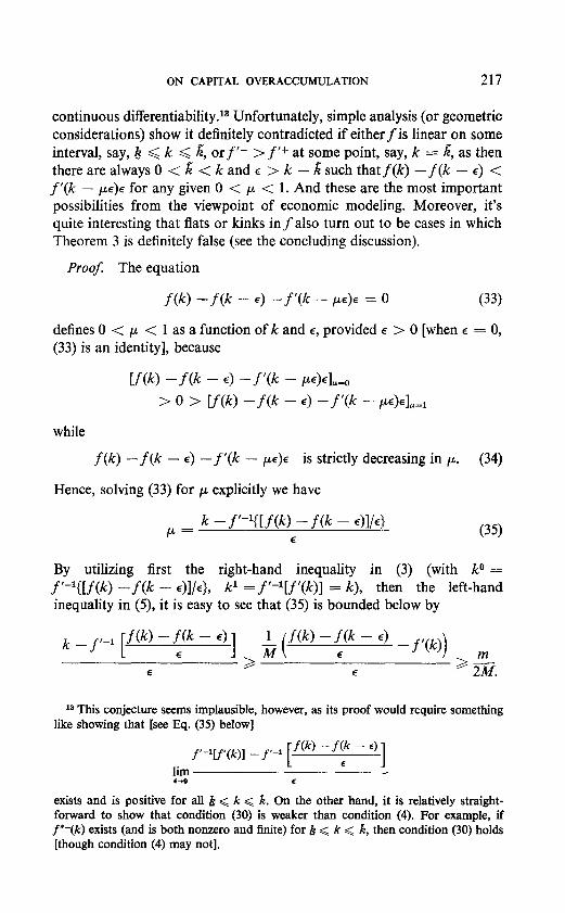
continuous differentiability. l3 Unfortunately, simple analysis (or geometric considerations) show it definitely contradicted if eitherfis linear on some interval, say, K < k < 6, orf’- > f ‘f at some point, say, k = 6, as then there are always 0 < K” < k and E > k - & such thatf(k) -f(k - c) < f ‘(k - ~E)E for any given 0 < p < 1. And these are the most important possibilities from the viewpoint of economic modeling. Moreover, it’s quite interesting that flats or kinks infalso turn out to be cases in which Theorem 3 is definitely false (see the concluding discussion).

Proof. The equation

f(k) --f(k - 6) --f’(k - ,LM)E = 0 (33)

defines 0 < p < 1 as a function of k and E, provided E > 0 [when E = 0, (33) is an identity], because

[f(k) -f(k - 4 --f’(k - ~blw=o > 0 > If(k) - f(k - E) --f’(k - /M)E]~=~

while

f-(k) - f(k - 4 --f’(k - ALE E > is strictly decreasing in CL. (34)

Hence, solving (33) for TV explicitly we have

~ = k - f’-W(k) - f(k - 4/4 E (35)

By utilizing first the right-hand inequality in (3) (with kO = f’-‘{[f(k) -f(k - 6)1/e}, k1 =f’-l[f’(k)] = k), then the left-hand inequality in (5), it is easy to see that (35) is bounded below by

k - f’-l [ fck) -f,‘” - “I > & (f(k) -;‘” - e> --J’(k)) 3 ~

I E E

la This conjecture seems implausible, however, as its proof would require something like showing that [see Eq. (35) below]

f’-‘[f’(k)l _ f’-l f(k) - f(k - 4

lim 1 E I

(4 c

exists and is positive for all & < k < R. On the other hand, it is relatively straight- forward to show that condition (30) is weaker than condition (4). For example, if f”-(k) exists (and is both nonzero and finite) for & < k < h, then condition (30) holds [though condition (4) may not].

218 CASS

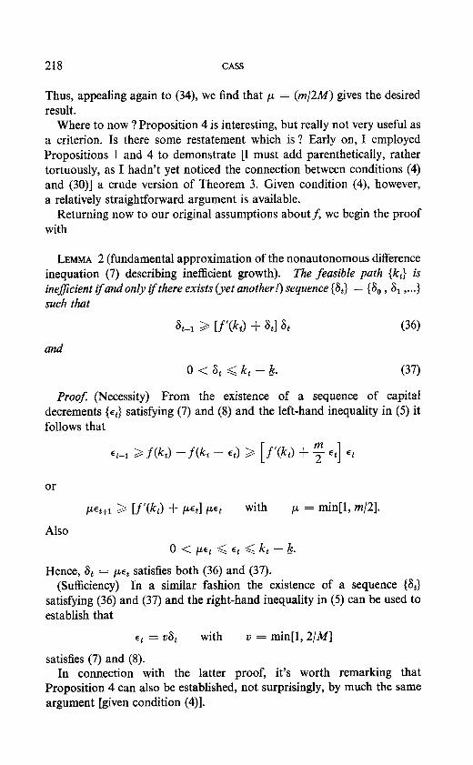
Thus, appealing again to (34), we find that p = (m/2M) gives the desired result.

Where to now ? Proposition 4 is interesting, but really not very useful as a criterion. Is there some restatement which is ? Early on, I employed Propositions 1 and 4 to demonstrate [I must add parenthetically, rather tortuously, as I hadn’t yet noticed the connection between conditions (4) and (30)] a crude version of Theorem 3. Given condition (4), however, a relatively straightforward argument is available.

Returning now to our original assumptions aboutf, we begin the proof with

LEMMA 2 (fundamental approximation of the nonautonomous difference inequation (7) describing inefficient growth). The feasible path {k,} is ineficient ifandonly if there exists (yet another!) sequence (6,) = (6, , 6, ,...} such that

at+1 2 V’W + %I At (36)

and

0 < St < kt - K. (37)

ProoJ (Necessity) From the existence of a sequence of capital decrements {et} satisfying (7) and (8) and the left-hand inequality in (5) it follows that

Et+1 2 f(kt) -f&t - 4 b [f’(k) + 7 et] l t

or

pet+1 2 V’(k) + ~4 wt with p = min[l, m/2].

Also

0 < pet d et < k, - k.

Hence, 6, = pet satisfies both (36) and (37). (Sufficiency) In a similar fashion the existence of a sequence (6,)

satisfying (36) and (37) and the right-hand inequality in (5) can be used to establish that

Et = us, with u = min[l, 2/M]

satisfies (7) and (8). In connection with the latter proof, it’s worth remarking that

Proposition 4 can also be established, not surprisingly, by much the same argument [given condition (4)].

ON CAPITAL OVERACCUMULATION 219

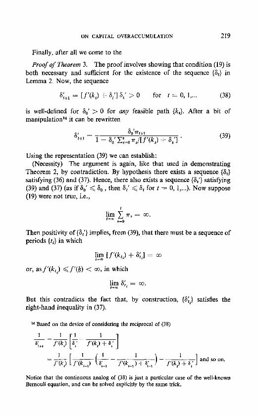
Finally, after all we come to the

Proof of Theorem 3. The proof involves showing that condition (19) is both necessary and sufficient for the existence of the sequence (S,} in Lemma 2. Now, the sequence

a;+1 = Lf’(Q + 4’1 4’ > 0 for f = 0, l,...

is well-defined for 6,’ > 0 for any feasible path {k,}. After a bit of manipulation14 it can be rewritten

a;+1 = SO’?,, 1 - 4,’ CL, ~,lLf’(k,) + %‘I ’ (39)

Using the representation (39) we can establish: (Necessity) The argument is again, like that used in demonstrating

Theorem 2, by contradiction. By hypothesis there exists a sequence (6,) satisfying (36) and (37). Hence, there also exists a sequence (S,‘} satisfying (39) and (37) (as if 6,’ < 6, , then 6,’ < 6, for t = 0, l,...). Now suppose (19) were not true, i.e.,

Then positivity of (6,‘) implies, from (39), that there must be a sequence of periods {ri} in which

$ LWt,) + S:J = ~0

or, as f’(k,J < f’(&) < co, in which

lim S;* = co. i-to2

But this contradicts the fact that, by construction, {S;i> satisfies the right-hand inequality in (37).

I4 Based on the device of considering the reciprocal of (38)

1 -=- 6’ t+1 I

Notice that the continuous analog of (38) is just a particular case of the well-known Bemouli equation, and can be solved explicitly by the same trick.

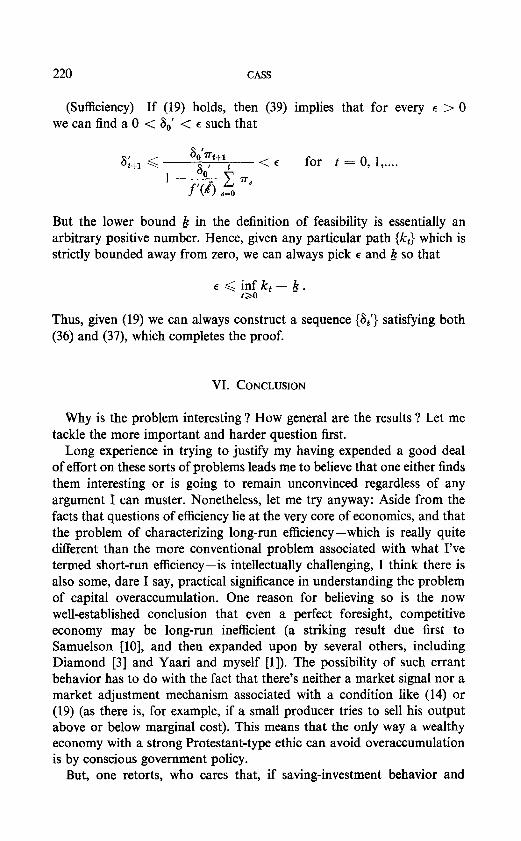
220 CASS

(Sufficiency) If (19) holds, then (39) implies that for every E > 0 we can find a 0 < 6,’ < z such that

&,I G &‘?+I a(+ <E

for t = 0, l,....

l - f@j ‘$=() ns

But the lower bound & in the definition of feasibility is essentially an arbitrary positive number. Hence, given any particular path {k,} which is strictly bounded away from zero, we can always pick E and & so that

Thus, given (19) we can always construct a sequence {S,‘} satisfying both (36) and (37), which completes the proof.

VI. CONCLUSION

Why is the problem interesting ? How general are the results ? Let me tackle the more important and harder question first.

Long experience in trying to justify my having expended a good deal of effort on these sorts of problems leads me to believe that one either finds them interesting or is going to remain unconvinced regardless of any argument I can muster. Nonetheless, let me try anyway: Aside from the facts that questions of efficiency lie at the very core of economics, and that the problem of characterizing long-run efficiency-which is really quite different than the more conventional problem associated with what I’ve termed short-run efficiency-is intellectually challenging, I think there is also some, dare I say, practical significance in understanding the problem of capital overaccumulation. One reason for believing so is the now well-established conclusion that even a perfect foresight, competitive economy may be long-run inefficient (a striking result due first to Samuelson [lo], and then expanded upon by several others, including Diamond [3] and Yaari and myself [l]). The possibility of such errant behavior has to do with the fact that there’s neither a market signal nor a market adjustment mechanism associated with a condition like (14) or (19) (as there is, for example, if a small producer tries to sell his output above or below marginal cost). This means that the only way a wealthy economy with a strong Protestant-type ethic can avoid overaccumulation is by conscious government policy.

But, one retorts, who cares that, if saving-investment behavior and

ON CAPITAL OVERACCUMULATION 221

production technology today are extrapolated forever, the economy would be missing some consumption opportunities? We can always have a consumption binge sometime in the future, however distant, and put matters aright, can’t we ? Indeed, we can, though there’s no quarantee that we will (and my personal preference is, when in doubt, favor the present against the future). More important, I can’t help but think one shouldn’t be too literal in interpreting the treatment of the indefinite future in our admittedly limited dynamic models. While the absence of a natural horizon for an economy combines with the great analytic advantage of considering asymptotic behavior, and more or less force us to think of the horizon as beyond any limit you care to name, what these models are really all about is at most the next 50,75,100 or perhaps even 150 years. Hence- and I only say this half jestingly-if I really thought the U.S. economy, for instance, were going to be significantly above the golden rule path for significantly long periods (very casual empiricism suggests we’re near there now -and even nearer if one takes the current concern with environmental problems seriously) I wouldn’t hesitate pressing for a much less expansionary growth policy.

But these are matters of opinion, and as I warned at the outset, my rambling probably won’t change anybody’s position. With regard to the second question posed, however, I can be somewhat more pointed.

There’s no doubt at all that the results catalogued in this paper depend crucially on having sufficient curvature and regularity to the boundary of the short-run intertemporal production possibility set (i.e., the set of consumption sequences corresponding to feasible growth paths which eventually maintain capital stocks at least as large as those on the feasible growth path whose long-run efficiency is in question). In particular, a close look at the proof of Theorem 3 reveals the following chains of implications: condition (19) * sequence (8,) satisfying (36) and (37), this + right-hand inequality in (5) => sequence {et> satisfying (7) and (8) * feasible path {k,} is inefficient 3 sequence {et} satisfying (7) and (8), this + left-hand inequality in (5) 3 sequence (6,) satisfying (36) and (37) * condition (19).

Thus, for example, (i) if the gross output function f has a kink at the golden rule capital stock R*, say,

f’-(L*) > 1 >f’+@*),

a path similar to (26)

k t+l - A* = A.‘(k,)(k, - A’*) with k, > A*, O<h<l

would satisfy (19) (as rrt <f’+(L*)“) but nevertheless be efficient (as lim,,, (k, - A*)/vrt = lim,,, At = 0 implies that any positive sequence

222 CASS

which satisfies (7) must eventually violate (8))-the right-hand inequality in (5) and thus sufficiency of (19) doesn’t obtain-while (ii) iffis linear at I*, say,

f’(k) > 1 for k < k < k*,=

= 1 k* < k < ;&*,

>l 7* < k,

any path

k, = k’ with k* < k’ < ;g*

is obviously inefficient though condition (14) and a fortiori condition (19) is not satisfied-the left-hand inequality in (5) and thus necessity of (19) doesn’t obtaiP.

This is disappointing, but hardly surprising; strong conclusions usually require strong assumptions. And, in any case, granted sufficient curvature and regularity-roughly, enough so that marginal rates of transformation between consumption today and tomorrow provide the basis for “good” second-order approximation to the economy’s short-run intertemporal production possibilities-I’m quite confident that condition (19) has a direct analog in a fairly general-in other respects, for instance, the number of commodities assumed-model of capitalistic production. But the investigation of this conjecture will be the subject of a future note.

REFERENCES

1. D. CASS AND M. E. YAARI, Individual saving, aggregate capital accumulation and efficient growth, in “Essays on the Theory of Optimal Economic Growth” (K. Shell, Ed.), Chap. 13, MIT Press, Cambridge, Mass., 1967.

2. D. CASS AND M. E. YAARI, Present values playing the role of efficiency prices in the one-good growth model, Rev. Econ. Studies 38 (1971), 331-339.

3. P. A. DIAMOND, National debt in a neoclassical growth model, The American Economic Review 55 (1965), 1126-1150.

4. E. MALINVAUD, Capital accumulation and efficient allocation of resources, Econo- metricu 21 (1953), 233-268.

I6 All bets are off if f is linear, say

f(k) = ak for k > 0.

In this case, it’s easily shown that (10) itself is both necessary and sufficient for ineffi- ciency, and easily seen that (19) always holds if a < 1, never holds if (I > 1.

I* It’s not critical that these examples revolve around the golden rule capital stock; the same results can be exhibited when a kink or flat occurs elsewhere.

ON CAPITAL OVERACCUMULATION 223

5. E. MALINVAUD, Efficient capital accumulation: a corrigendum, Econometrica, 30 (1962), 570-573.

6. B. PELEG AND M. E. YAARI, Efficiency prices in an infinite-dimensional space, J. Econ. Theory, 2 (1970), 41-85.

7. E. S. PHELPS, Second essay on the golden rule of accumulation, Amer. Econ. Rev., 55 (1965), 783-814.

8. E. S. FHEZLPS, “Golden Rules of Economic Growth,” pp. 55-68, Norton, New York, 1966.

9. R. RADNER, Efficiency prices for infinite horizon production programs, 34 (1967), 51-66.

10. P. A. SAMUELSON, An exact consumption-loan model of interest with or without the social contrivance of money, .7. Pol. Econ., 66 (1958), 467-482.