On chassis predictive maintenance and service solutions ...

Department of Mechanics and Maritime Sciences CHALMERS UNIVERSITY OF TECHNOLOGY Gothenburg, Sweden 2019

On chassis predictive maintenance and service solutions:

An unsupervised machine learning approach

Master’s thesis in Complex Adaptive Systems

NASTARAN SOLTANIPOUR

Master’s thesis in Complex Adaptive Systems

On chassis predictive maintenance and service solutions:

An unsupervised machine learning approach


Department of Mechanics and Maritime Sciences

Division of Vehicle Engineering and Autonomous Systems

Vehicle Dynamics group

CHALMERS UNIVERSITY OF TECHNOLOGY

Gothenburg, Sweden 2019

On chassis predictive maintenance and service solutions: An unsupervised machine

learning approach


© NASTARAN SOLTANIPOUR, 2019

Supervisor: Sadegh Rahrovani (Volvo cars), John Martinsson (Rise),

Mats Jonasson (Chalmers university), Robin Westlund (Volvo cars)

Examiner: Bengt J H Jacobson

Master’s Thesis 2019:41




Chalmers University of Technology

SE-412 96 Gothenburg

Sweden

Telephone: + 46 (0)31-772 1000

On chassis predictive maintenance and service solutions: An unsupervised machine

learning approach





Chalmers University of Technology

Abstract

Predictive maintenance is a key component in cost reduction in automotive industry

and is of great importance. Besides cutting the costs, predictive maintenance can

improve feeling of comfort and safety, by early detection, isolation and prediction of

prospective failures. That is why automotive industry and fleet managers are turning to

predictive analytics to maintain a lead position in industry. In order to predict and

mitigate components failure in advance, measurements data from vehicle parts are

collected from sensory system mounted on vehicle parts, and employed to evaluate the

health condition of the components. An unsupervised learning solution is proposed, in

this work, for automatic processing, diagnosis and isolation of faults. This solution is

used for advanced analytics of the collected time-series data in the back-end (assuming

that faults were reported based on spectral analysis). A literature study on maintenance

types with emphasis on predictive maintenance with application to chassis failure is

done. Chassis failures and conventional failure detection techniques are also covered in

this study.

A data acquisition was done at Hällared test track and labelled data regarding error

states of interest were collected. Performance of the proposed method was validated by

automatics clustering of two error states, i.e. low tyre pressure and faulty wheel hub.

Key words: predictive maintenance, chassis failure detection, unsupervised machine

learning

Acknowledgements

My sincere thanks to my main supervisors Sadegh Rahrovani (Volvo Cars) and John

Martinson (RISE) for their guidance and great ideas on diagnostics, predictive

maintenance and Machine Learning topics, during my master thesis project. I also

express my gratitude towards my university supervisor Mats Jonasson (Vehicle

dynamics group, Chalmers), Bengt Jacobsson (Vehicle dynamics group, Chalmers) and

Robin Westlund (Volvo Cars) for their valuble feedbacks on my thesis draft, Last, but

not least, I would like to thank my manager at Volvo Car Corporation, Georgios Minos,

for giving an opportunity to work with him and his team as a thesis student. I would

also like to thank my family and friends, for their moral support for finishing my thesis.

- Nastaran Soltanipour

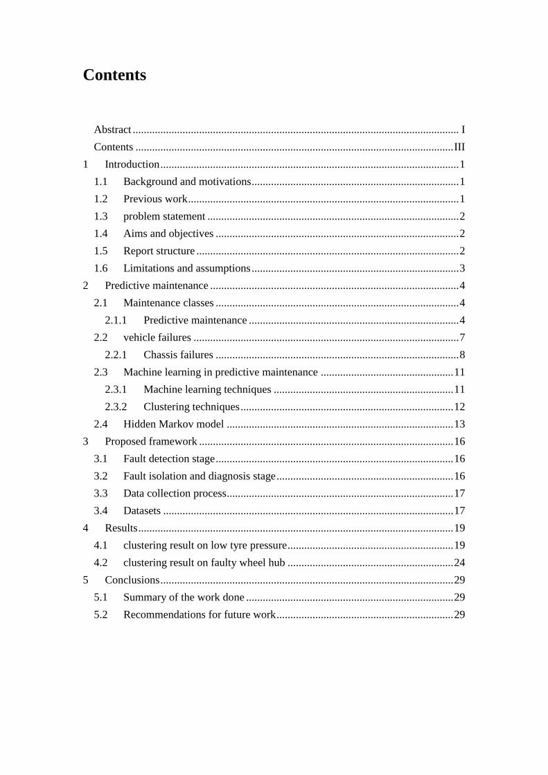
Contents

Abstract ...................................................................................................................... I

Contents ................................................................................................................... III

1 Introduction ............................................................................................................ 1

1.1 Background and motivations ........................................................................... 1

1.2 Previous work .................................................................................................. 1

1.3 problem statement ........................................................................................... 2

1.4 Aims and objectives ........................................................................................ 2

1.5 Report structure ............................................................................................... 2

1.6 Limitations and assumptions ........................................................................... 3

2 Predictive maintenance .......................................................................................... 4

2.1 Maintenance classes ........................................................................................ 4

2.1.1 Predictive maintenance ............................................................................ 4

2.2 vehicle failures ................................................................................................ 7

2.2.1 Chassis failures ........................................................................................ 8

2.3 Machine learning in predictive maintenance ................................................ 11

2.3.1 Machine learning techniques ................................................................. 11

2.3.2 Clustering techniques ............................................................................. 12

2.4 Hidden Markov model .................................................................................. 13

3 Proposed framework ............................................................................................ 16

3.1 Fault detection stage ...................................................................................... 16

3.2 Fault isolation and diagnosis stage ................................................................ 16

3.3 Data collection process .................................................................................. 17

3.4 Datasets ......................................................................................................... 17

4 Results .................................................................................................................. 19

4.1 clustering result on low tyre pressure ............................................................ 19

4.2 clustering result on faulty wheel hub ............................................................ 24

5 Conclusions .......................................................................................................... 29

5.1 Summary of the work done ........................................................................... 29

5.2 Recommendations for future work ................................................................ 29

CHALMERS, Mechanics and Maritime Sciences, Master’s Thesis 2019:41 1

1 Introduction

1.1 Background and motivations

Maximizing reliability while keeping the costs down is the key strategy to ensure a

leading position in automotive industry. To satisfy these requirements is it essential to

develop a framework capable of detecting, isolating and predicting of the prospective

failures of the system to ensure reliability of the system as well as cutting the costs of

repair or replacement of the components. Predictive maintenance is the key solution to

this issue. Predictive maintenance is a condition-based monitoring and maintenance

planning solution in which periodic or continuous evaluations of the system is

conducted to prevent possible failures of the system. Assessments can be conducted on

stored data from data clouds or historic datasets.

Data-driven descriptive and predictive approaches provides us powerful tools to detect,

identify and characterize potential system failure modes during operation. These can be

directly used for both root-cause analysis (to help system designers to design failure-

free designs) and predictive analytics (to help system maintenance/service to

diagnose/identify failures based on the unique signatures of each individual) of the

potential failure modes in the operation. Machine learning techniques are being spread

for service and maintenance solutions, which will be discussed more in the following

literature study part. This thesis propose a machine learning based solution for

automizing the process of classifiying and clustering of differente errors, after they are

detected in the onboard-diagnostic. This, together with detailed discussion about the

advantages and limitations of the methods will be discussed in the following.

1.2 Previous work

Considering the above-mentioned issues, the Climate and Motion Control Department

(former Vehicle Control and Chassis – Strategy, Innovation and Integration group),

within the Research & Development at Volvo Cars, started to investigate & expand the

pallet of data analytics and machine learning tools for the purpose of chassis error state

detection, monitoring, and maintenance solutions. These advance engineering and

method development projects, started from early 2018, resulted in a patent application

that was filed under patent Number 16/410,850 [1]. In brief, it consists of three

packages:

1) Real-time fault detection solution in an on board diagnosis system, via an spectrum

analysis solution.

2) A solution (i.e. a supervised Tree-based machine learning approach) for finding

features/signals that are important for classification and root cause analysis of

faults/errors of interest. The output of this analysis guides the design/improvement of

both detection stage (1) and also isolation/diagnostic for the offline solutions in the

back-end in stage (2).

2 CHALMERS, Mechanics and Maritime Sciences, Master’s Thesis 2019:41

3) Automating the process of fault isolation, clustering and diagnostics via an

unsupervised machine learning approach.

This thesis scope is to address the third stage of the-above mentioned patent application.

This thesis contributes there, by proposing an Hidden Markov Model-based sequence

tagging approach that enables us to automatically annotate/label the collected

fault/error data in order to reduce the high amount of cost in labelling of time-series

that corresponds to different faults/error states.

1.3 Problem statement

Managers of car sharing and taxi service fleets, are turning to predictive analytics to

stay on top of maintenance and predict and mitigate components failure, in advance.

Sensors on vehicles collect data for assessing the health of different systems and

components. Particularly speaking about chassis, these sensors gather information

regarding tyre pressure, wheel hub bearings, hydraulics in the dampers, brakes and so

on. However, process of analysis of vehicle sensors in order to diagnose and isolate the

faults is an expensive task. The main focus of this thesis is to address this issue by

proposing an unsupervised machine learning solution for fault clustering as well as

differing different error states as different classes.

1.4 Aims and objectives

This thesis project aims at:

• Literature study on data-driven tools for predictive maintenance solutions in

automotive industry.

• Analysis of the available test data, including data cleaning/labelling for creating

ground truth labelling of error states of interests. (Collection of more test data, in case

needed). Collection and analysis of data concerns low tyre pressure, faulty/noisy wheel

hub, and faulty damper error states.

• Develop and apply unsupervised Machine Learning tools for automating the

analysis of collected time-series data, to conduct chassis failures detection.

• Using the collected test data (with ground truth labels), validate the performance

of the method and results compilation.

1.5 Report structure

The rest of the report is organized as follows: chapter two is dedicated to literature

study, mainly discussing different maintenance methods, with the main focus on

predictive maintenance, main approaches in predictive maintenance, such as vibration

analysis and machine learning approach. Study of different failures occurring in chassis

and different machine learning approaches to address clustering problems.


Chapter three discusses the physical phenomenon describing low tyre pressure and

faulty wheel hub as well as a brief history of existing detection techniques. Also and

the proposed algorithm, data acquisition and data processing is described in this

chapter.

Chapter four represent the results from low tyre pressure detection, and isolation of

faulty wheel hub and low tire pressure states in form of figures, tables and confusion

matrices

Chapter five is dedicated to the summary of the thesis, conclusions and proposals for

the future works in chassis failure detection techniques.

1.6 Limitations and assumptions

The dataset employed in this study contains the normal driving state as well as data

collected from the car while driving on faulty components. We assume that the error

states are isolated and known and the data is collected from proper road surface

conditions with no pothole or roughness. The data is not reflecting neither the error

states occurring simultaneously in the car nor the transient phases between the normal

and faulty states. The datasets collected from test tracks are stored in predefined

circumstances and since the procedure of repeating the test is time consuming and needs

access to the proving ground the data is limited to 4 different speed levels, three test

tracks, and three different states, one normal and two faulty. On the other hand the test

has been conducted in only one vehicle and one set of tire.


2 Predictive maintenance

2.1 Maintenance and service solutions

Over the course of years numerous maintenance methods have been proposed and

employed in industries. All these methods share a common goal: increasing

productivity and quality while preventing failure as well as limiting the downtime. All

different maintenance methods fall into two main categories, namely: scheduled and

unscheduled maintenance categories[2].

The first class of maintenance is corrective maintenance also known as “Run-to-

Failure” and “Breakdown Maintenance”. This type of maintenance is conducted when

the machine suffers a breakdown or malfunction. This also can lead to multiple

damages to the equipment or the system. This type of maintenance can be significantly

expensive due to repair and replacement costs alongside with non-productive duration

of downtime of the equipment[3]. It is estimated that only in US the cost of corrective

maintenance every year is more than 200 million dollars which can be prevented with

the help of more intelligent approaches[2].

Preventive maintenance is the second approach in maintenance classes which is a type

of scheduled maintenance. Preventive maintenance tends to prevent failures, safety

violation situations, production losses, unnecessary repairs, and aims to preserve

original materials and equipment. This can be achieved by replacing the consumables

at predefined time intervals and conducting regular time-based inspection of the system

as well as identifying the rate of failures in the system[4].

The last and the most advanced maintenance and the most cost effective method is

predictive maintenance. In this method the data from sensory system is evaluated

continuously to find the trends in the data to assess the health of the system as well as

to predict the prospective failures of the system. This is discussed more in the next

following section[5].

2.1.1 Predictive maintenance

Predictive maintenance is generally described simply as estimation of the optimal time

for performing maintenance on the system. In predictive maintenance the ultimate goal

is to detect failure before they occur.

Predictive maintenance is capable and efficient in detection of the possible failures

during early stages, which leads to decrease in unscheduled downtime. Shorter

downtime means increase in productivity as well as quality and safety improvement.

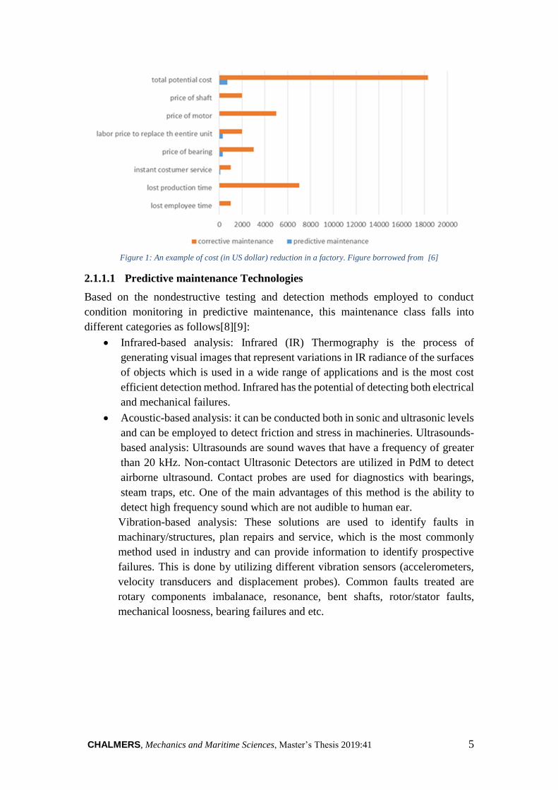
Predictive maintenance is capable of significant reduction of cost in industry.

According to McKinsey Global Institute, predictive maintenance can save up to $200

billion to $600 billion for manufacturers by year 2025[6]. Figure (1) depicts an example

of a comparison between corrective and predictive maintenance methods.

Predictive maintenance has become feasible, thanks to lower sensor prices and wireless

data acquisition and data delivery mechanisms such as telematics and data clouds.


Figure 1: An example of cost (in US dollar) reduction in a factory. Figure borrowed from [6]

2.1.1.1 Predictive maintenance Technologies

Based on the nondestructive testing and detection methods employed to conduct

condition monitoring in predictive maintenance, this maintenance class falls into

different categories as follows[8][9]:

• Infrared-based analysis: Infrared (IR) Thermography is the process of

generating visual images that represent variations in IR radiance of the surfaces

of objects which is used in a wide range of applications and is the most cost

efficient detection method. Infrared has the potential of detecting both electrical

and mechanical failures.

• Acoustic-based analysis: it can be conducted both in sonic and ultrasonic levels

and can be employed to detect friction and stress in machineries. Ultrasounds-

based analysis: Ultrasounds are sound waves that have a frequency of greater

than 20 kHz. Non-contact Ultrasonic Detectors are utilized in PdM to detect

airborne ultrasound. Contact probes are used for diagnostics with bearings,

steam traps, etc. One of the main advantages of this method is the ability to

detect high frequency sound which are not audible to human ear.

Vibration-based analysis: These solutions are used to identify faults in

machinary/structures, plan repairs and service, which is the most commonly

method used in industry and can provide information to identify prospective

failures. This is done by utilizing different vibration sensors (accelerometers,

velocity transducers and displacement probes). Common faults treated are

rotary components imbalanace, resonance, bent shafts, rotor/stator faults,

mechanical loosness, bearing failures and etc.


2.1.1.2 Predictive maintenance approaches

Figure 2: Predictive maintenance methods based on monitoring techniques. Figure borrowed from review paper

[9]

This section is dedicated to the main approaches in predictive maintenance, there are

three main categories in condition monitoring techniques, namely: Data methods,

Model Based Methods, and Knowledge Based Methods. Data based method employ

available historical data to conduct failure detection. Principal component analysis

(PCA) is an instance of such methods in which orthogonal transformations are

employed to diminish the dimension of possible correlated observations to a reduced

number of uncorrelated variables. In fact PCA is a dimension reduction method which

makes it easier to process and monitor large dimensional datasets. Fault detection can

be conducted by change detection in the converted data[10].

The main idea in model based methods is to compare the actual measured output of the

system with the output from the mathematical model. State observer method is a model

based method functioning upon this fact that changes in input-output behavior directly

affect the state variables of the state space model. State observer can be employed for

fault detection if it is possible to model the error as changes in state variables[10].

Figure 3: State observer detection structure [9]

Knowledge Based Methods are feasible when experts and experience is available.

However acquiring deep understanding of a system is costly and hard if not impossible.

Fuzzy logic is a knowledge based system that is capable of providing different level of

severity of the fault in the alarm system. In figure (2) different detection methods are

introduced[10].

Monitoring techniques

Data based

Spectrum analysis

Principle componant

analysis

Machine Learning

based

Model based

State observers

Parameter estimation

Knowledge based

Expert system

Fuzzy systems


All the methods above fall into two broader categories as: rule based methods and

machine learning methods. Rule based maintenance also known as condition

monitoring is the continuous analysis of the sensory data for triggering an alarm signal

upon a predefined rule or threshold. In this method once the common reasons for system

failure are stablished having the model of the system network, engineers can build up a

set of “if- then” rule to control the behavior and interdependencies of the system. Like

fuzzy logic and spectrum analysis methods like fast Fourier transform[11].

Though these systems provide some level of autonomy to the system, still these sort of

predictive maintenance algorithms need expert knowledge to derive the rules based on

the system requirements [11].

Unlike rule based methods, in machine learning methods the historical data or data from

online clouds are fed as inputs to a number of different algorithms namely:

classification and clustering algorithms, pattern recognition systems using neural

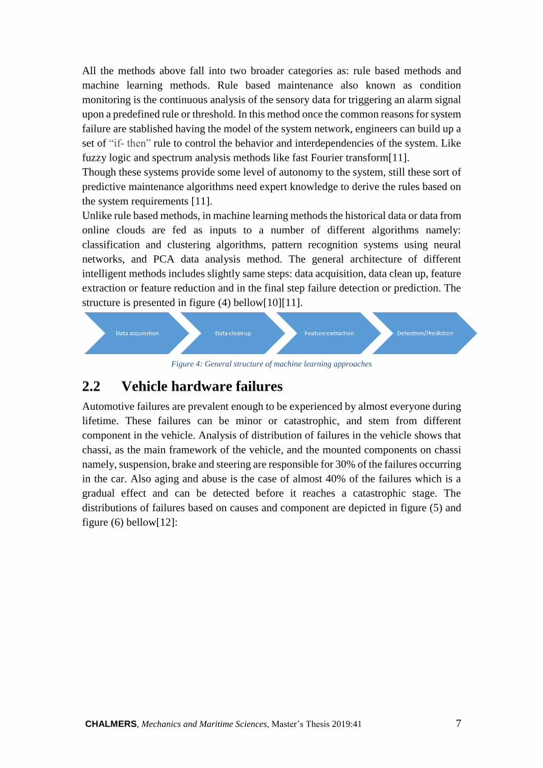
networks, and PCA data analysis method. The general architecture of different

intelligent methods includes slightly same steps: data acquisition, data clean up, feature

extraction or feature reduction and in the final step failure detection or prediction. The

structure is presented in figure (4) bellow[10][11].

Figure 4: General structure of machine learning approaches

2.2 Vehicle hardware failures

Automotive failures are prevalent enough to be experienced by almost everyone during

lifetime. These failures can be minor or catastrophic, and stem from different

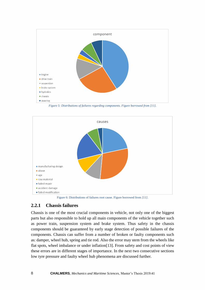
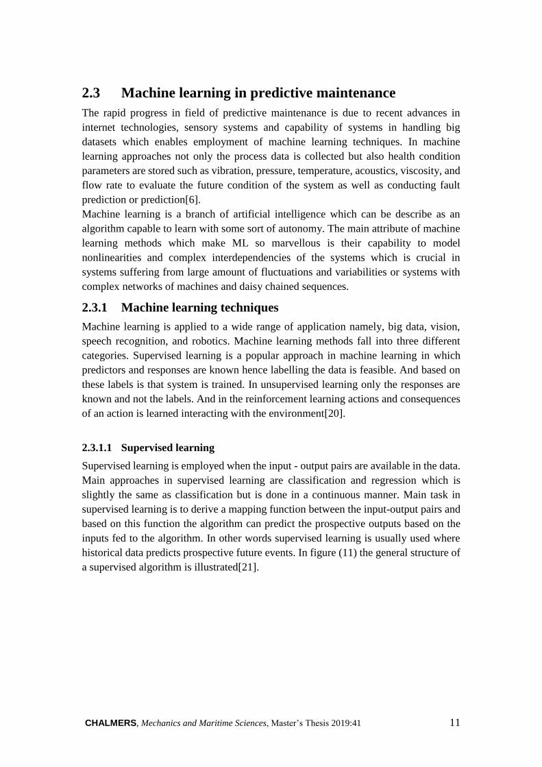
component in the vehicle. Analysis of distribution of failures in the vehicle shows that

chassi, as the main framework of the vehicle, and the mounted components on chassi

namely, suspension, brake and steering are responsible for 30% of the failures occurring

in the car. Also aging and abuse is the case of almost 40% of the failures which is a

gradual effect and can be detected before it reaches a catastrophic stage. The

distributions of failures based on causes and component are depicted in figure (5) and

figure (6) bellow[12]:


Figure 5: Distributions of failures regarding components. Figure borrowed from [11].

Figure 6: Distributions of failures root cause. Figure borrowed from [11].

2.2.1 Chassis failures

Chassis is one of the most crucial components in vehicle, not only one of the biggest

parts but also responsible to hold up all main components of the vehicle together such

as power train, suspension system and brake system. Thus safety in the chassis

components should be guaranteed by early stage detection of possible failures of the

components. Chassis can suffer from a number of broken or faulty components such

as: damper, wheel hub, spring and tie rod. Also the error may stem from the wheels like

flat spots, wheel imbalance or under inflation[13]. From safety and cost points of view

these errors are in different stages of importance. In the next two consecutive sections

low tyre pressure and faulty wheel hub phenomena are discussed further.


2.2.2 Investigated chassis failure

The main focus in this thesis is to develop a detection method capable of detecting and

isolating low tire pressure and faulty wheel hub error states since both can lead to

catastrophic circumstances in vehicles if not detected and also both low tyre pressure

and faulty wheel hub can have similar effects on vibration analysis that makes it

difficult to isolate the errors using conventional detection techniques.

2.2.2.1 Low tire pressure

A tire is a rubber structure reinforced with nylon fabrics and metal steel belts[14]. Tires

can be modelled as springs with stiffness depending on the direction the load is applied

in this sense each tire will have its specific stiffness that is directly related to the level

of inflation of the tire. Higher pressures inducing higher stiffness and vice versa[15].

The spring model is depicted bellow:

Figure 7: The spring model of the tire

In this model mass is the un-sprung mass which is mainly weight of the parts not

supported by the suspension system, namely: wheels, wheels axle and all components

connected to them. In some studies in the literature tire is modeled considering the

damping effect too but the simplified model we are using here considers only the spring

which is sensitive to tire pressure level[15].

Figure 8: Effect of different Inflation levels on tire figure borrowed from [16].

Distribution of vehicle weight on the tire, thus stability of the vehicle is directly related

to the level of inflation of the tires. Over or under inflation can affect handling of the

car as well as cornering and stopping. An over or under inflated tire wear out unevenly

and faster which increases the repair expenses. Under inflated tires are slower in

response hence affects the normal performance of the vehicle as well as safety. Over

inflated tires become stiffer and influence the road-tire contact which in turn causes

noise and make the vehicle more prone to tar roads and potholes[16]. In figure (8) the

effect of over and under inflation on the tire is depicted.


2.2.2.2 Faulty wheel bearing

Faulty wheel hub is a state of the hub which can occur due to faults stemming from hub

units. Wheel hub components are vulnerable to aging and wear out over the course of

time. Hub bearing is one of the essential components in wheel hub which can cause

speed dependant noise upon being worn. Wheel bearing can fail due to damages on the

rollers surface or the bearing race. The roller and the race surfaces are both polished so

precisely to let roller pass easily over the race but over time the bearing wears slightly

causing microscopic metal particles into the bearing grease. Metal particles ae well as

any other kind of contamination causes deformation of the surfaces. Since the bearing

are subjected to so much weight even on very small deformations of the surface it can

cause a lot of noise[17]. In figure (9) a wheel hub is depicted.

Figure 9: Wheel hub schematic

In wheel hub bearing, each ball bearing can be modelled as a set of parallel springs and

dampers[18]. Any deformation in the ball bearing can change the stiffness and damping

of the system which can lead to changes in frequency response of the system. Spring-

damper model of a bearing is depicted bellow:

Figure 10: Wheel bearing spring-damper model

Wheel hub bearing is crucial in safety and handling characteristics of the vehicle. It

enables the car to turn freely and plays an important role in smoothness of the ride and

fuel consumption as well as performance of ABS brake system. If the wheel bearing

wears out leads to increase in the friction and cause the wheel to wobble[17].


2.3 Machine learning in predictive maintenance

The rapid progress in field of predictive maintenance is due to recent advances in

internet technologies, sensory systems and capability of systems in handling big

datasets which enables employment of machine learning techniques. In machine

learning approaches not only the process data is collected but also health condition

parameters are stored such as vibration, pressure, temperature, acoustics, viscosity, and

flow rate to evaluate the future condition of the system as well as conducting fault

prediction or prediction[6].

Machine learning is a branch of artificial intelligence which can be describe as an

algorithm capable to learn with some sort of autonomy. The main attribute of machine

learning methods which make ML so marvellous is their capability to model

nonlinearities and complex interdependencies of the systems which is crucial in

systems suffering from large amount of fluctuations and variabilities or systems with

complex networks of machines and daisy chained sequences.

2.3.1 Machine learning techniques

Machine learning is applied to a wide range of application namely, big data, vision,

speech recognition, and robotics. Machine learning methods fall into three different

categories. Supervised learning is a popular approach in machine learning in which

predictors and responses are known hence labelling the data is feasible. And based on

these labels is that system is trained. In unsupervised learning only the responses are

known and not the labels. And in the reinforcement learning actions and consequences

of an action is learned interacting with the environment[20].

2.3.1.1 Supervised learning

Supervised learning is employed when the input - output pairs are available in the data.

Main approaches in supervised learning are classification and regression which is

slightly the same as classification but is done in a continuous manner. Main task in

supervised learning is to derive a mapping function between the input-output pairs and

based on this function the algorithm can predict the prospective outputs based on the

inputs fed to the algorithm. In other words supervised learning is usually used where

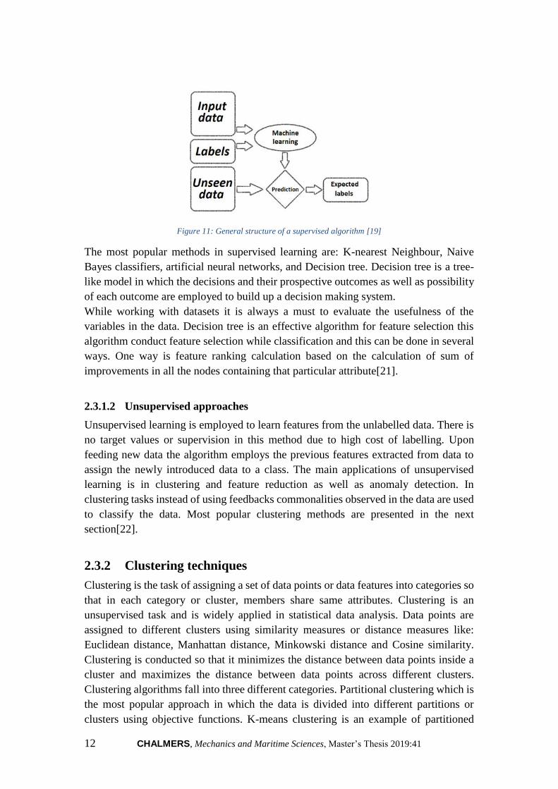
historical data predicts prospective future events. In figure (11) the general structure of

a supervised algorithm is illustrated[21].


Figure 11: General structure of a supervised algorithm [19]

The most popular methods in supervised learning are: K-nearest Neighbour, Naive

Bayes classifiers, artificial neural networks, and Decision tree. Decision tree is a tree-

like model in which the decisions and their prospective outcomes as well as possibility

of each outcome are employed to build up a decision making system.

While working with datasets it is always a must to evaluate the usefulness of the

variables in the data. Decision tree is an effective algorithm for feature selection this

algorithm conduct feature selection while classification and this can be done in several

ways. One way is feature ranking calculation based on the calculation of sum of

improvements in all the nodes containing that particular attribute[21].

2.3.1.2 Unsupervised approaches

Unsupervised learning is employed to learn features from the unlabelled data. There is

no target values or supervision in this method due to high cost of labelling. Upon

feeding new data the algorithm employs the previous features extracted from data to

assign the newly introduced data to a class. The main applications of unsupervised

learning is in clustering and feature reduction as well as anomaly detection. In

clustering tasks instead of using feedbacks commonalities observed in the data are used

to classify the data. Most popular clustering methods are presented in the next

section[22].

2.3.2 Clustering techniques

Clustering is the task of assigning a set of data points or data features into categories so

that in each category or cluster, members share same attributes. Clustering is an

unsupervised task and is widely applied in statistical data analysis. Data points are

assigned to different clusters using similarity measures or distance measures like:

Euclidean distance, Manhattan distance, Minkowski distance and Cosine similarity.

Clustering is conducted so that it minimizes the distance between data points inside a

cluster and maximizes the distance between data points across different clusters.

Clustering algorithms fall into three different categories. Partitional clustering which is

the most popular approach in which the data is divided into different partitions or

clusters using objective functions. K-means clustering is an example of partitioned


clustering which starts with random initializing of cluster centres. In the next step using

distance equations each data point is assigned to the closest centre and then the

consecutive new centres are calculated using averaging over all dimensions. Until the

improvement in each step falls down a predefined value. Though this method is fast

and requires low computational cost, the number of clusters is chosen by user and it

does not necessarily represent the true number of clusters in the data. Other partitional

clustering method is hidden Markov model which will be discussed thoroughly in next

section[23].

The other approach is Density based Clustering. In this method clusters are defined as

regions where the density of the data point exceeds a predefined value. DBSCAN is an

example of density based clustering. Hierarchical Clustering is the last method which

tends to divide or merge partitions in the data to form optimal number of clusters.

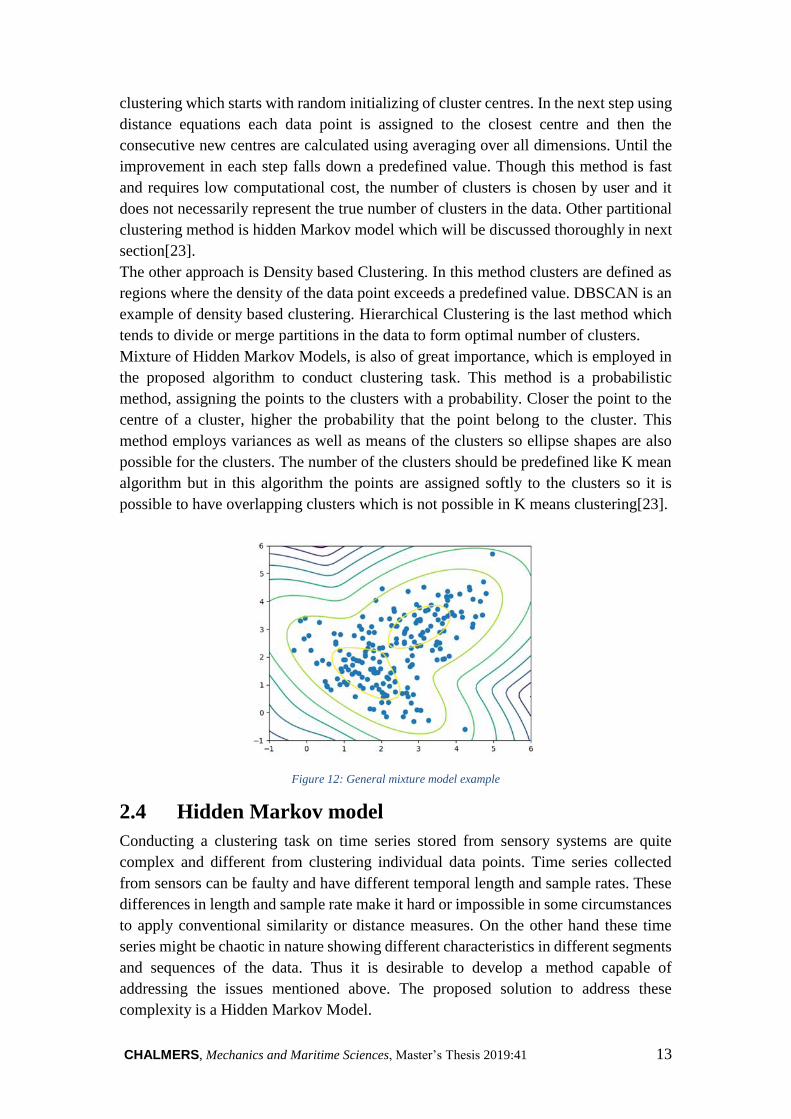
Mixture of Hidden Markov Models, is also of great importance, which is employed in

the proposed algorithm to conduct clustering task. This method is a probabilistic

method, assigning the points to the clusters with a probability. Closer the point to the

centre of a cluster, higher the probability that the point belong to the cluster. This

method employs variances as well as means of the clusters so ellipse shapes are also

possible for the clusters. The number of the clusters should be predefined like K mean

algorithm but in this algorithm the points are assigned softly to the clusters so it is

possible to have overlapping clusters which is not possible in K means clustering[23].

Figure 12: General mixture model example

2.4 Hidden Markov model

Conducting a clustering task on time series stored from sensory systems are quite

complex and different from clustering individual data points. Time series collected

from sensors can be faulty and have different temporal length and sample rates. These

differences in length and sample rate make it hard or impossible in some circumstances

to apply conventional similarity or distance measures. On the other hand these time

series might be chaotic in nature showing different characteristics in different segments

and sequences of the data. Thus it is desirable to develop a method capable of

addressing the issues mentioned above. The proposed solution to address these

complexity is a Hidden Markov Model.


A Hidden Markov Model is a statistical model developed for systems that evolve

through a finite number of states. It is assumed that the observations of these systems

are generated by a hidden stochastic process which can be model using a Markov chain.

This hidden states can be decoded by analysing the observations of the system to

determine probabilistically which state the system is in. Hidden Markov models have

been used successfully in a wide range of applications such as: body gesture

recognition, sign language interpretation as well as time series analysis[24].

In a hidden Markov model a sequence of observations 𝑂 = { 𝑂1, 𝑂2, … 𝑂𝑛} are

generated by an unknown hidden process. Each observation is the result of a specific

hidden state represented as: 𝑋 = {𝑋1, 𝑋2, … . 𝑋𝑚} . Considering the hidden Markov

model as 𝜆 = {Π, 𝛼, 𝛽} where Π is the initial probability of each state showing how

probable it is for a new input sequence to start from a particular state, α is the state

transition matrix defining the probability of moving from one hidden state to another

and β is the observation matrix and is the probability of each observation to be the result

of a particular state. The sum of all start probabilities is equal to one as well as the sum

of elements in each row in the transition probability matrix. An example of hidden

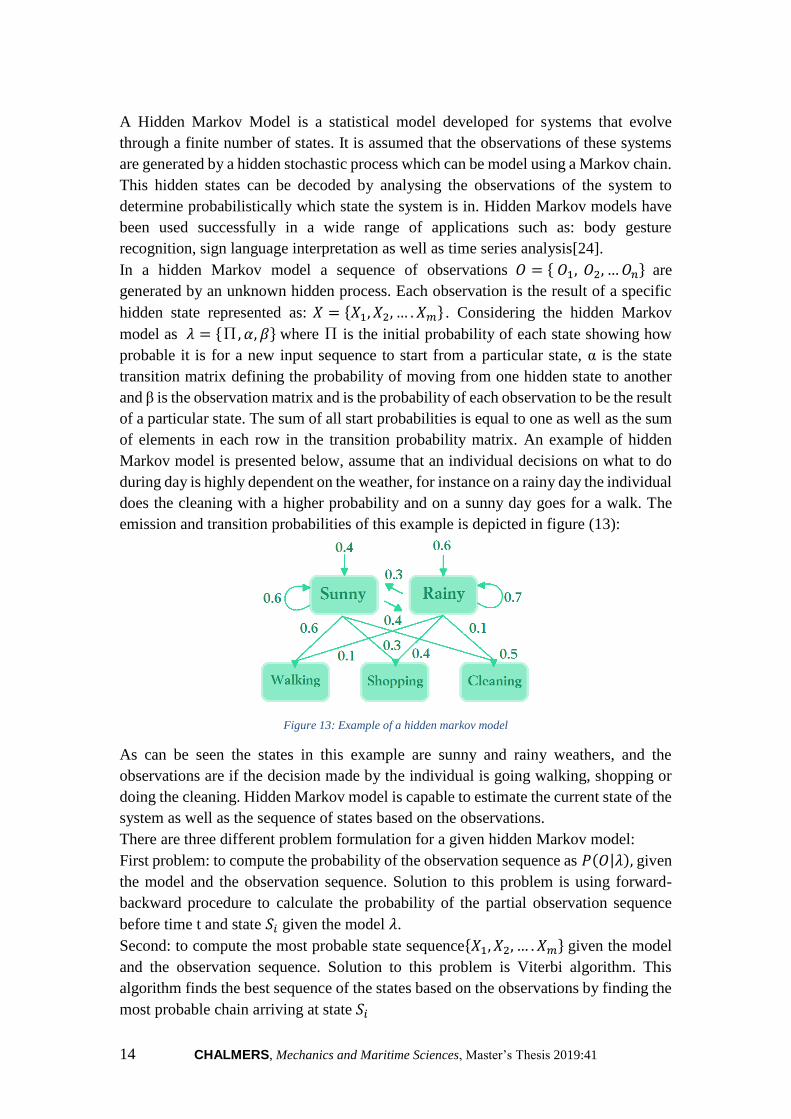
Markov model is presented below, assume that an individual decisions on what to do

during day is highly dependent on the weather, for instance on a rainy day the individual

does the cleaning with a higher probability and on a sunny day goes for a walk. The

emission and transition probabilities of this example is depicted in figure (13):

Figure 13: Example of a hidden markov model

As can be seen the states in this example are sunny and rainy weathers, and the

observations are if the decision made by the individual is going walking, shopping or

doing the cleaning. Hidden Markov model is capable to estimate the current state of the

system as well as the sequence of states based on the observations.

There are three different problem formulation for a given hidden Markov model:

First problem: to compute the probability of the observation sequence as 𝑃(𝑂|𝜆), given

the model and the observation sequence. Solution to this problem is using forward-

backward procedure to calculate the probability of the partial observation sequence

before time t and state 𝑆𝑖 given the model 𝜆.

Second: to compute the most probable state sequence{𝑋1, 𝑋2, … . 𝑋𝑚} given the model

and the observation sequence. Solution to this problem is Viterbi algorithm. This

algorithm finds the best sequence of the states based on the observations by finding the

most probable chain arriving at state 𝑆𝑖


Third: model parameter selection to maximize probability of the observation

sequence𝑃(𝑂|𝜆). Though there is no optimal solution for this problem it is possible to

choose 𝜆 = {Π, 𝛼, 𝛽} such that it is locally minimized using Baum-Welch algorithm.

This algorithm starts by assigning random probabilities and adjust them later on such

that the probability that the model assigns to the training set is maximized[24].

2.4.5. Model selection

As mentioned in section (2.3.1.1) dedicated to unsupervised clustering methods, in

majority of the methods, the number of clusters is assumed to be known. This

assumption is usually made upon observing the data. Nevertheless, for high

dimensional datasets where a visual realization of the data is impossible or in complex

datasets with overlapping clusters, assuming the number of clusters if not impossible is

hard. Thus some model selection algorithms are proposed in the literature to find the

optimal number of clusters in the data. The Bayesian information criterion (BIC) is a

criteria for selecting the optimal model among a finite number of possible models. The

model is selected which produces the lowest BIC. BIC criteria is defined as follows:

𝐵𝐼𝐶 = ln(𝑛) 𝑘 − 2ln (𝐿) (1)

In this equation L is the maximum likelihood function of the model which is described

as the plausibility of a value for the parameter, given some data. 𝑘 is the number of free

parameters in the model, such as: number of states in each hidden Markov model,

number of hidden Markov models in the mixture model, and the mixture models gains,

and n is the number of inputs fed to the algorithm. In this thesis BIC is employed for

model selection[25].


3 Proposed framework

3.1 Fault detection stage

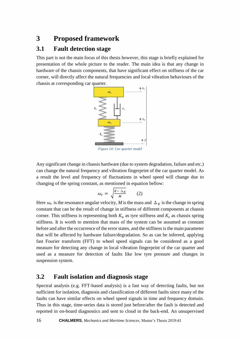
This part is not the main focus of this thesis however, this stage is briefly explained for

presentation of the whole picture to the reader. The main idea is that any change in

hardware of the chassis components, that have significant effect on stiffness of the car

corner, will directly affect the natural frequencies and local vibration behaviours of the

chassis at corresponding car quarter.

Figure 14: Car quarter model

Any significant change in chassis hardware (due to system degradation, failure and etc.)

can change the natural frequency and vibration fingerprint of the car quarter model. As

a result the level and frequency of fluctuations in wheel speed will change due to

changing of the spring constant, as mentioned in equation bellow:

𝜔𝑟 = √𝐾− Δ𝐾

𝑀 (2)

Here 𝜔𝑟 is the resonance angular velocity, M is the mass and Δ𝐾 is the change in spring

constant that can be the result of change in stiffness of different components at chassis

corner. This stiffness is representing both 𝐾𝑢 as tyre stiffness and 𝐾𝑠 as chassis spring

stiffness. It is worth to mention that mass of the system can be assumed as constant

before and after the occurrence of the error states, and the stiffness is the main parameter

that will be affected by hardware failure/degradation. So as can be inferred, applying

fast Fourier transform (FFT) to wheel speed signals can be considered as a good

measure for detecting any change in local vibration fingerprint of the car quarter and

used as a measure for detection of faults like low tyre pressure and changes in

suspension system.

3.2 Fault isolation and diagnosis stage

Spectral analysis (e.g. FFT-based analysis) is a fast way of detecting faults, but not

sufficient for isolation, diagnosis and classification of different faults since many of the

faults can have similar effects on wheel speed signals in time and frequency domain.

Thus in this stage, time-series data is stored just before/after the fault is detected and

reported in on-board diagnostics and sent to cloud in the back-end. An unsupervised


learning solution is adopted, in this thesis, for automatic fault isolation/diagnosis, for

the purpose of more efficient and lower cost predictive/descriptive solutions for service

and maintenance in the back-end. This method is proposed in [28] for clustering

Vehicle Maneuver Trajectories The performance of the method is validated by

diagnosis of two different error states, i.e. low tyre pressure and faulty wheel hub, using

the collected data at test track. A mixture of hidden Markov models is employed in

order to conduct clustering task, where the configuration of the model is specified by a

model selection procedure, based on BIC model selection criteria [29]. To achieve this,

the experiment is repeated for different number of hidden states and different number

of Markov models in the mixture model. The model yielding smallest value of BIC is

chosen. The initial emission and transient probabilities are chosen randomly which is

updated and optimized during the training process. In this experiment forward

algorithm is employed to calculate the log probability of the model. The whole dataset

is fed to the algorithm for training since no verification was needed due to unsupervised

nature of training algorithm.

In this thesis unsupervised learning is employed to give the algorithm the freedom to

detect as many clusters as there are in the data since the actual number of fault clusters

is unknown in real world applications.

3.3 Data collection process

The time series are collected from flex-ray of a V90 Volvo passenger car. First the data

is examined for possible corrupted data and the data is cleaned up from empty runs and

corrupted data then labelled based on different states of driving this labelling system is

employed for the verification of the method and is not used in a supervised manner as

targets. Then data is sorted based on different driving profiles so the functionality of

the method can be evaluated in different driving modes such as: turns and straight

forwards.

3.4 Datasets

The datasets are collected by Volvo Car Corporation in Hällered proving ground in

Sweden. The tests are conducted on different test tracks for three different

circumstances. One state represents normal driving situation, the other state is 25%

under inflation in one wheel then test is repeated for a faulty wheel hub. The tire

pressure initially is set to 275 kPa for nominal inflated pressure for normal driving test

and then reduced to 220kpa for low tyre pressure test. Data acquisition frequency is set

to 100 Hertz.

First dataset is collected from the vehicle conducting a test on the country road test

track which is straight forward driving track. This track contains no curve and no bump

and there was an intention to keep the speed constant throughout the test to minimize

the effect of other interfering factors. Country road data-set contains normal, low tyre

pressure and faulty wheel hub states.


The second dataset is collected from handling road test track, which contains moderate

turning and uphill and downhill driving. The dataset contains time series collected from

normal, low tire pressure and faulty wheel hub tests. Each test is conducted for two

different scenarios: one scenario is to log the data at fixed spped of 60 Kmph and the

other scenario is to log data when the vehicle starts with 30 Kmph but then elevate the

speed to 60 Kmph and then in the next step elevate the spped to 80 Kmph in order to

include the effect of acceleration in the dataset. Then both scenarios are repeated for

two trials.

City traffic test track is the last track we have used for collecting data. Since there is a

speed limit for this test track due to sharp turns, the data set only contains one speed

level and time series on normal and low tire pressure. For each state the experiment is

repeated twice.

The manouvers where selected in different test tracks to log the data needed to

investigate different situation excited in the chassis and tyres the list of signals

investigated is as bellow:

Front left wheel speed 30kmph Front right wheel speed 30kmph Rear right wheel speed

30kmph

Rear left wheel speed 30kmph

Front left wheel speed 60kmph Front right wheel speed60kmph Rear right wheel speed

60kmph



80kmph



100kmph


Table 1:Speed levels of speed signals fed tp the algorithm


4 Results

4.1 Fault diagnosis result for low tyre pressure

We evaluated the functionality of our proposed algorithm using the low tyre pressure

and normal driving from the three datasets described in the previous section. As

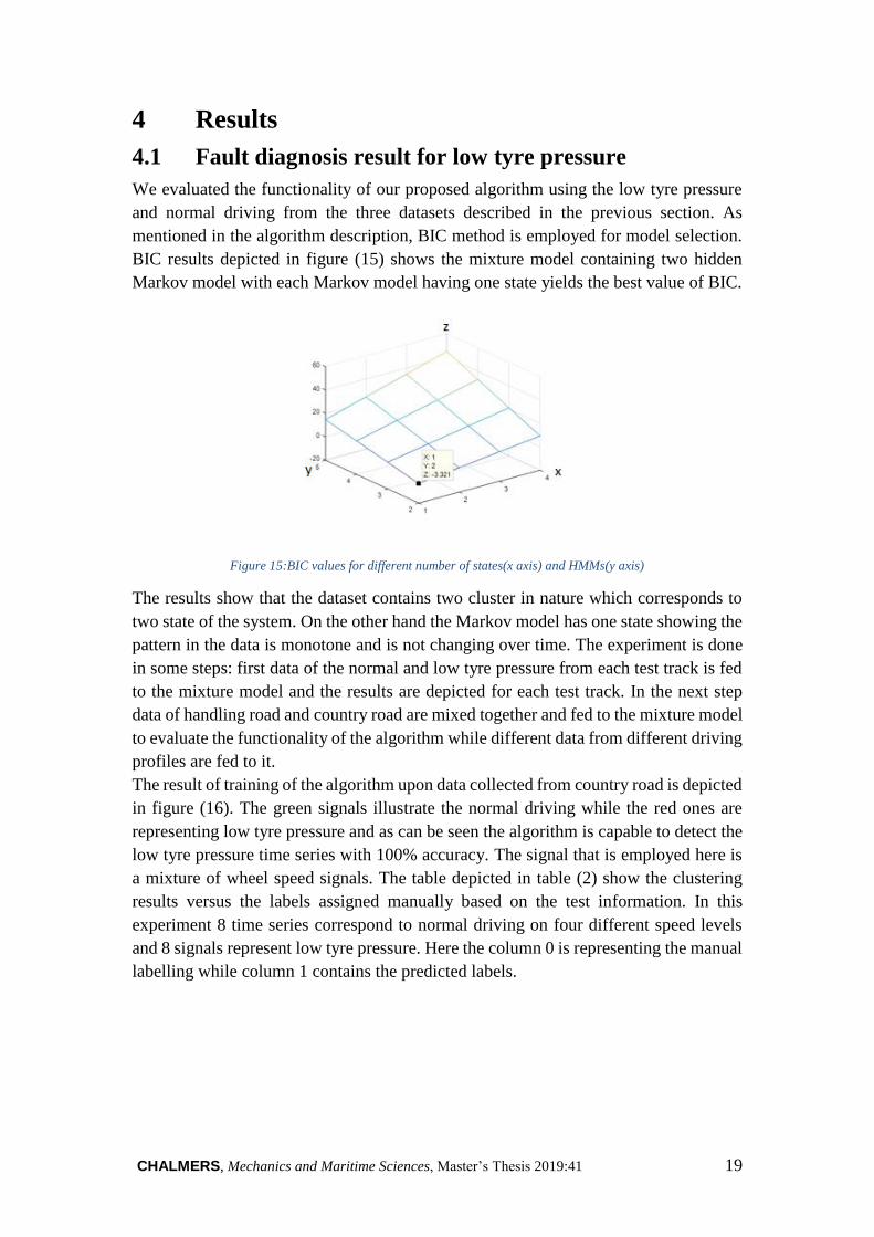
mentioned in the algorithm description, BIC method is employed for model selection.

BIC results depicted in figure (15) shows the mixture model containing two hidden

Markov model with each Markov model having one state yields the best value of BIC.

Figure 15:BIC values for different number of states(x axis) and HMMs(y axis)

The results show that the dataset contains two cluster in nature which corresponds to

two state of the system. On the other hand the Markov model has one state showing the

pattern in the data is monotone and is not changing over time. The experiment is done

in some steps: first data of the normal and low tyre pressure from each test track is fed

to the mixture model and the results are depicted for each test track. In the next step

data of handling road and country road are mixed together and fed to the mixture model

to evaluate the functionality of the algorithm while different data from different driving

profiles are fed to it.

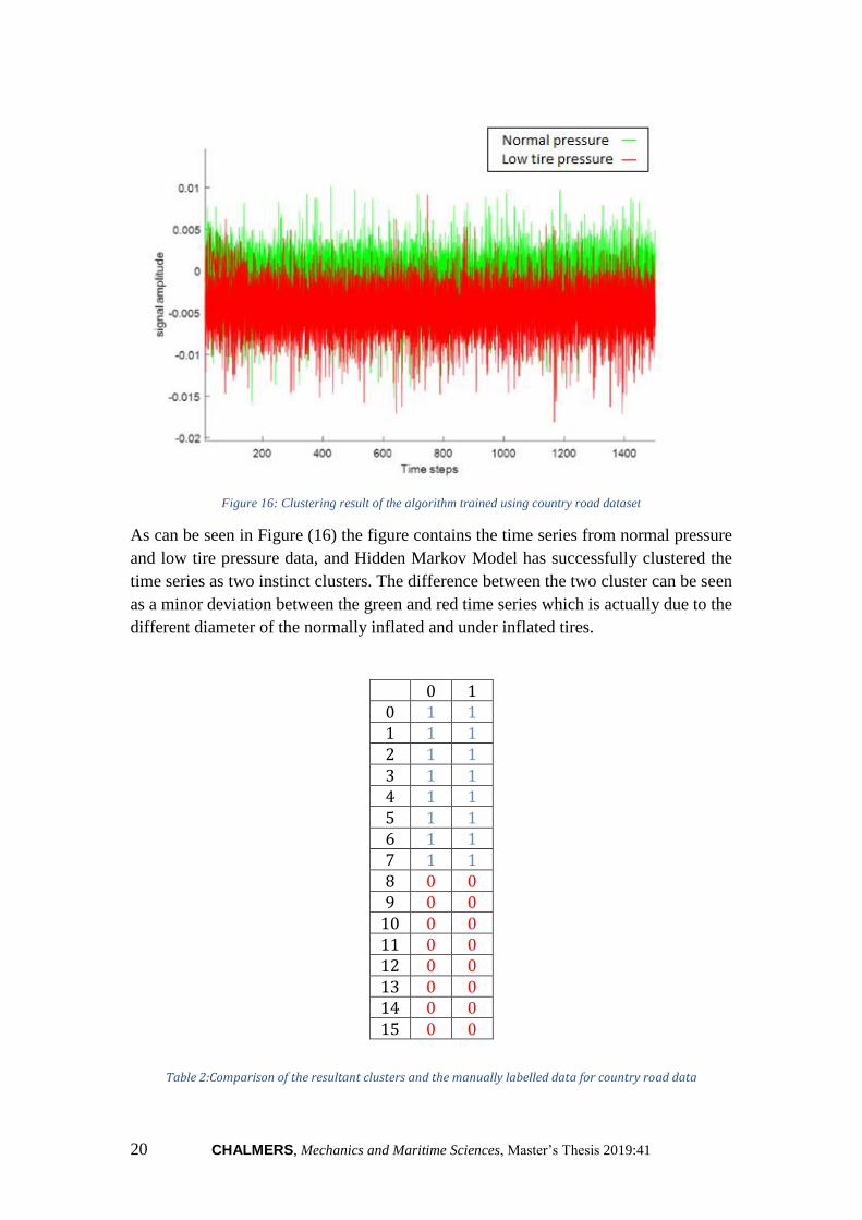
The result of training of the algorithm upon data collected from country road is depicted

in figure (16). The green signals illustrate the normal driving while the red ones are

representing low tyre pressure and as can be seen the algorithm is capable to detect the

low tyre pressure time series with 100% accuracy. The signal that is employed here is

a mixture of wheel speed signals. The table depicted in table (2) show the clustering

results versus the labels assigned manually based on the test information. In this

experiment 8 time series correspond to normal driving on four different speed levels

and 8 signals represent low tyre pressure. Here the column 0 is representing the manual

labelling while column 1 contains the predicted labels.


Figure 16: Clustering result of the algorithm trained using country road dataset

As can be seen in Figure (16) the figure contains the time series from normal pressure

and low tire pressure data, and Hidden Markov Model has successfully clustered the

time series as two instinct clusters. The difference between the two cluster can be seen

as a minor deviation between the green and red time series which is actually due to the

different diameter of the normally inflated and under inflated tires.

0 1 0 1 1 1 1 1 2 1 1 3 1 1 4 1 1 5 1 1 6 1 1 7 1 1 8 0 0 9 0 0

10 0 0 11 0 0 12 0 0 13 0 0 14 0 0 15 0 0

Table 2:Comparison of the resultant clusters and the manually labelled data for country road data


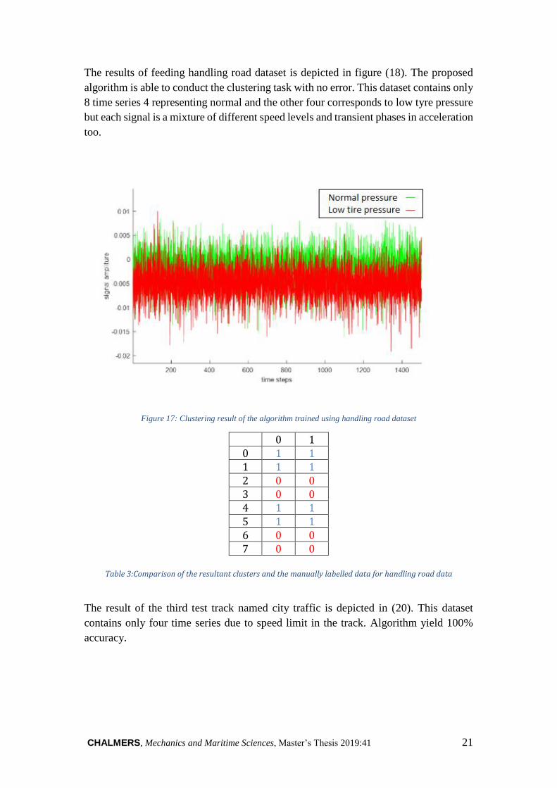
The results of feeding handling road dataset is depicted in figure (18). The proposed

algorithm is able to conduct the clustering task with no error. This dataset contains only

8 time series 4 representing normal and the other four corresponds to low tyre pressure

but each signal is a mixture of different speed levels and transient phases in acceleration

too.

Figure 17: Clustering result of the algorithm trained using handling road dataset

0 1 0 1 1 1 1 1 2 0 0 3 0 0 4 1 1 5 1 1 6 0 0 7 0 0

Table 3:Comparison of the resultant clusters and the manually labelled data for handling road data

The result of the third test track named city traffic is depicted in (20). This dataset

contains only four time series due to speed limit in the track. Algorithm yield 100%

accuracy.


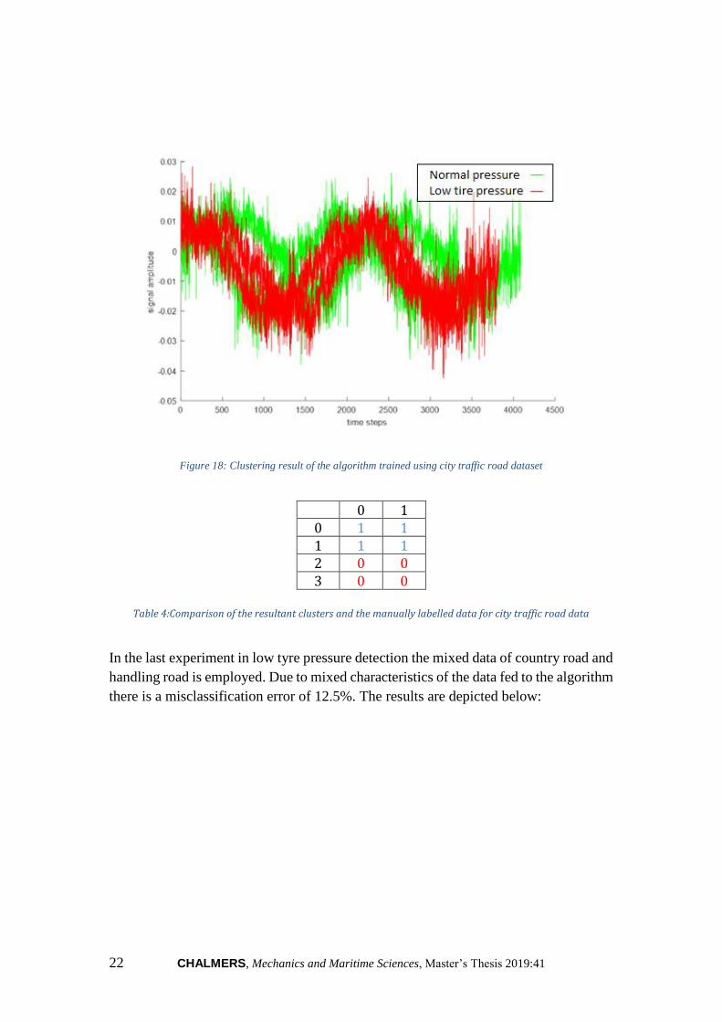
Figure 18: Clustering result of the algorithm trained using city traffic road dataset

0 1

0 1 1 1 1 1 2 0 0 3 0 0

Table 4:Comparison of the resultant clusters and the manually labelled data for city traffic road data

In the last experiment in low tyre pressure detection the mixed data of country road and

handling road is employed. Due to mixed characteristics of the data fed to the algorithm

there is a misclassification error of 12.5%. The results are depicted below:


Figure 19: Clustering result of the algorithm trained using Handling road and country road data

0 1 0 1 1 1 1 1 2 1 1 3 1 1 4 1 1 5 1 1 6 1 1 7 1 1 8 1 0 9 1 0 10 0 0 11 1 0 12 0 0 13 0 0 14 0 0 15 0 0 16 1 1 17 1 1 18 0 0 19 0 0 20 1 1 21 1 1 22 0 0 23 0 0

Table 5:Comparison of the resultant clusters and the manually labelled data for handling road and country road data


As can be seen from the table (24) three time series out of 24 time series are

misclassified. The algorithm could not detect the low tyre pressure for two time series

out of 12 time series corresponding to low tyre pressure and also sends out low tire

pressure warning when no error has occurred. The results are summarised in the

contingency matrix bellow:

Figure 20: Contingency matrix of the mixed data clustering result

Regarding the contingency some evaluation metrics are calculated as bellow: the table

shows the number of true negative, true positive and false alarms.

Sensitivity of the system also known as detection rate and true positive rate is 100%.

Sensitivity is the portion of errors detected among the number of errors actually

occurred in the system. Specificity of the system is 75% which is the proportion of

actual negatives that are correctly identified also known as true negative rate. Accuracy

of the system 87.5% which is the capability of the algorithm to assign the time series to

the right cluster.

4.2 Fault diagnosis result for faulty wheel hub

The algorithm employed to detect faulty wheel hub is exactly similar to the algorithm

utilized to detect low tyre pressure. The model selection procedure for faulty wheel hub

yields same configuration with two hidden Markov model and one hidden state in each

model. The result of BIC method for model selection is illustrated in figure (25).

Figure 21: BIC values for different number of states(x axis) and HMMs(y axis)


The experiment is conducted for country road and handling test tracks. Figure (26)

depicts the results for faulty wheel hub detection conducted on handling test tracks. The

dataset contains 4 time series representing faulty wheel hub and the other four

correspond to low tyre pressure.

Figure 22: Clustering result of the algorithm trained using Handling road data

0 1

0 1 1 1 1 1 2 1 1 3 1 1 4 0 0 5 0 0 6 0 0 7 0 0

Table 6:Comparison of the resultant clusters and the manually labelled data for handling road data

The experiment is repeated for country road test track and the results are depicted in

figure (28) as can be seen the algorithm is capable of isolating faulty wheel hub from

low tyre pressure with 100% accuracy.


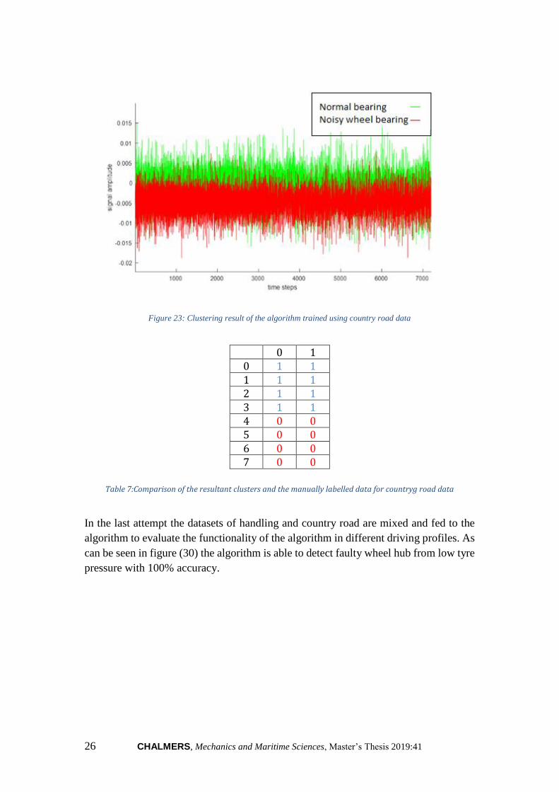
Figure 23: Clustering result of the algorithm trained using country road data

0 1 0 1 1 1 1 1 2 1 1 3 1 1 4 0 0 5 0 0 6 0 0 7 0 0

Table 7:Comparison of the resultant clusters and the manually labelled data for countryg road data

In the last attempt the datasets of handling and country road are mixed and fed to the

algorithm to evaluate the functionality of the algorithm in different driving profiles. As

can be seen in figure (30) the algorithm is able to detect faulty wheel hub from low tyre

pressure with 100% accuracy.


Figure 24: Clustering result of the algorithm trained using country road and handling road data

0 1 0 1 1 1 1 1 2 1 1 3 1 1 4 1 1 5 1 1 6 1 1 7 1 1 8 0 0 9 0 0

10 0 0 11 0 0 12 0 0 13 0 0 14 0 0 15 0 0

Table 8:Comparison of the resultant clusters and the manually labelled data for countryg road and handling

road data

The summary of the results on faulty wheel hub is depicted in the confusion matrix

bellow.


Figure 25: Contingency matrix of the mixed data clustering result

Based on the contingency matrix specificity, sensitivity and accuracy of the system is

100%.


5 Conclusions

5.1 Summary of the work done

Chassis failure detection is crucial regarding safety and maintenance costs. It is also

vital for automotive companies to address the issue to be able to maintain a leading

position in the industry, so detection and prevention of such failures is of great

importance. In this thesis a novel machine learning method for chassis failure detection

was proposed.

First data collected from the test tracks was investigated and cleaned up from corrupted

data and empty runs, and labelled using Mat-lab software. Then the data was fed to the

unsupervised machine learning algorithm developed in pomegranate library in python

which was a mixture model of hidden Markov models.

The experiment was conducted for low tyre pressure detection as well as isolating of

low tyre pressure from faulty wheel hub for different datasets. The algorithm was

capable to detect low tyre pressure with 100% accuracy for handling, country road, and

city traffic road, and yield 87.5% accuracy when employed for a mixture of different

driving profiles. The results of isolating faulty wheel hub from low tyre pressure were

more promising where the algorithm was capable to detect faulty wheel hub with 100%

accuracy for all datasets as well as mixed dataset.

5.2 Recommendations for future work

Next step to enhance this method can be collecting a new dataset containing transient

states of the signals from different driving scenarios as well as different speeds and

different road conditions so the algorithm can be trained upon a broad range of data that

can lead to better understanding of effect of different conditions on the algorithm such

as effect of turns or rough roads. On the other hand the data is logged from a particular

vehicle and this can effect the robustness of the algorithm in the future we aim to train

the algorithm based on the data logged form different vehicles.

In this thesis the proposed method has been applied to detect individual error states,

such as low tyre pressure and faulty wheel hub. The other track for future work can be

applying this method to detect different error states as well as mixed errors as a separate

state of the system. In this situation algorithm will be trained to detect clusters that are

representing combination of different errors.


6 References

[1]

[2]

Westlund R., Rahrovani S., Tyagi P., Soltanipour, N., Patent Application No.

16/410,850 filed on 05/13/2019 in United States: “Machine Learning Based

Vehicle Diagnostics And Maintenance ”

N. Amruthnath and T. Gupta, “Fault Class Prediction in Unsupervised Learning

using Model-Based Clustering Approach,” Conference Proceedings of 2018

International Conference on Information and Computer Technologies [3] D. L. D. B. Andrew K.S. Jardine, “A review on machinery diagnostics and

prognostics implementing condition-based maintenance,” Mechanical Systems

and Signal Processing, 2006.

[4] M. Kenneth, N. Octavian and M. William, “Prognostics and Health Management

in the Oil & Gas Industry,” Europian Confrence Of The Prognosis And Health

Managment Society, 2018.

[5] A. K. Verma, A. Patwardhan and U. Kumar, “A Survey on Predictive

Maintenance Through Big Data,” Current Trends in Reliability, Availability,

Maintainability and Safety: An Industry Perspective, pp. 437-445, 2016.

[6] Mckinsey global institute, “The Internet Of Things: Mapping The Value Behind

The Hype” 2015.

[7] ExcellentBlog, “6 benefits of using predictive maintenance,” data analysis from

soliton. Available:

https://reliabilityweb.com/tips/article/the_top_6_benefits_of_predictive_mainten

ance/.[Accessed 5 may 2019].

[8] L. Robin, “Slick tricks in oil analysis,” plant services, 2006.

[9] L. Jay, W. Fangji, G. Masoud, L. Linxia and S. David, “Prognostics and health

management design for rotary machinery systems—Reviews, methodology and

applications,” Mechanical Systems and Signal Processing, 2013.

[10] D. Miljković, “Fault Detection Methods: A Literature Survey,” researchgate,

2016.

[11] P. Jahnke, “Machine Learning Approaches for Failure Type Detection and

Predictive Maintenance,” Department of Computer Science, Darmstadt,

Germany, 2015.

[12] M. A, “Automotive Component Failures,” Elsevier Science Ltd, Great Britain,

1998.

[13] D. Couchman, “what-components-of-the-suspension-or-steering-systems-are-

prone-to-fail,” your mechanic inc, 17 november 2015. [Online]. Available:

https://www.yourmechanic.com/article/what-components-of-the-suspension-or-

steering-systems-are-prone-to-fail. [Accessed 5 may 2019].

[14] “How is a tire made,” Michelin us, [Online]. Available:

https://www.michelinman.com/US/en/help/how-is-a-tire-made.html.

[15] L. Jiao, “Vehicle model for tyre-ground,” Department of Aeronautical and

Vehicle Engineering KTH Royal Institute of Technology, stockholm, 2013.

[16] “Tire Pressure Monitoring System (TPMS),” [Online]. Available:

http://mytpms.blogspot.com/.


[17] A. Varghese, “Influence of Tyre Inflation Pressure on Fuel Consumption, Vehicle

Handling and Ride Quality,” Chalmers University Of Technology, Gothenburg,

2013.

[18] SKF, “What is a wheel hub bearing and why is it critical to your safety?”, 2012.

[19] J. A. Grajales, J. F. López and H. F. Quintero, “Ball bearing vibrations model:

Development and experimental validation,” SciELO, vol. vol.16 no.2, 2014.

[20] R. N. B. Kajaree Das, “A Survey on Machine Learning: Concept, Algorithms and

Applications,” International Journal of Innovative Research in Computer, Vols.

Vol. 5, Issue 2, 2017.

[21] S. J. P. A. U. Uma Narayanan, “A survey on various supervised classification

algorithms,” in 2017 International Conference on Energy, Communication, Data

Analytics and Soft Computing (ICECDS), Chennai,India .

[22] M. K. Memoona Khanum, “A Survey on Unsupervised Machine Learning

Algorithms for Automation, Classification and Maintenance,” Volume 119 –

No.13, June 2015.

[23] Y. T. Dongkuan Xu, “A Comprehensive Survey of Clustering Algorithms,”

Springer-Verlag Berlin Heidelberg, 2015.

[24] S. S. a. V. Patil, “Hidden Markov Model as Classifier: A survey,” Computer

Science and Engineering , 2013.

[25] “wikipedia,” [Online]. Available:

https://en.wikipedia.org/wiki/Hidden_Markov_model. [Accessed 1th September

2019].

[26] S. M. F. S. T. R. a. B. G. A. Frank J. Fabozzi, “Appendix.E,” in Model Selection

Criterion: AIC and BIC techniques, 2014.

[27] M. H. R. B. Dieter Schramm, Vehicle Dynamics: Modeling and Simulation,

Springer, 2014th Edition.

[28] J. Martinsson, N. Mohammadiha and A. Schliep, “Clustering Vehicle Maneuver

Trajectories Using Mixtures of Hidden Markov,” in 2018 21st International

Conference on Intelligent Transportation Systems (ITSC).

[29] C. Fraley and A. E. Raftery, “How Many Clusters? Which Clustering Method?

Answers Via Model-Based Cluster Analysis,” The Computer Journal, vol. 41, no.

8, pp. 578 - 588, 1998.

[30] “Slick tricks in oil analysis,” Lana,Robin, 2006.

Date post:	24-Feb-2022
Category:	Documents
Upload:	others
View:	1 times
Download:	0 times

On chassis predictive maintenance and service solutions ...

Documents