ON CHOOSING AND BOUNDING PROBABILITYMETRICS

ALISON L. GIBBS AND FRANCIS EDWARD SU

Manuscript version January 2002

Abstract. When studying convergence of measures, an important is-sue is the choice of probability metric. We provide a summary and somenew results concerning bounds among some important probability met-rics/distances that are used by statisticians and probabilists. Knowledgeof other metrics can provide a means of deriving bounds for another onein an applied problem. Considering other metrics can also provide alter-nate insights. We also give examples that show that rates of convergencecan strongly depend on the metric chosen. Careful consideration is nec-essary when choosing a metric.

Abrege. Le choix de metrique de probabilite est une decision tresimportante lorsqu’on etudie la convergence des mesures. Nous vousfournissons avec un sommaire de plusieurs metriques/distances de prob-abilite couramment utilisees par des statisticiens(nes) at par des proba-bilistes, ainsi que certains nouveaux resultats qui se rapportent a leursbornes. Avoir connaissance d’autres metriques peut vous fournir avec unmoyen de deriver des bornes pour une autre metrique dans un problemeapplique. Le fait de prendre en consideration plusieurs metriques vouspermettra d’approcher des problemes d’une maniere differente. Ainsi,nous vous demontrons que les taux de convergence peuvent dependre defacon importante sur votre choix de metrique. Il est donc important detout considerer lorsqu’on doit choisir une metrique.

1. Introduction

Determining whether a sequence of probability measures converges is acommon task for a statistician or probabilist. In many applications it isimportant also to quantify that convergence in terms of some probabilitymetric; hard numbers can then be interpreted by the metric’s meaning,and one can proceed to ask qualitative questions about the nature of thatconvergence.

Key words and phrases. discrepancy, Hellinger distance, probability metrics, Prokhorovmetric, relative entropy, rates of convergence, Wasserstein distance.

First author supported in part by an NSERC postdoctoral fellowship. Second authoracknowledges the hospitality of the Cornell School of Operations Research during a sab-batical in which this was completed. The authors thank Jeff Rosenthal and Persi Diaconisfor their encouragement of this project and Neal Madras for helpful discussions.

1

2 ALISON L. GIBBS AND FRANCIS EDWARD SU

Abbreviation MetricD DiscrepancyH Hellinger distanceI Relative entropy (or Kullback-Leibler divergence)K Kolmogorov (or Uniform) metricL Levy metricP Prokhorov metricS Separation distance

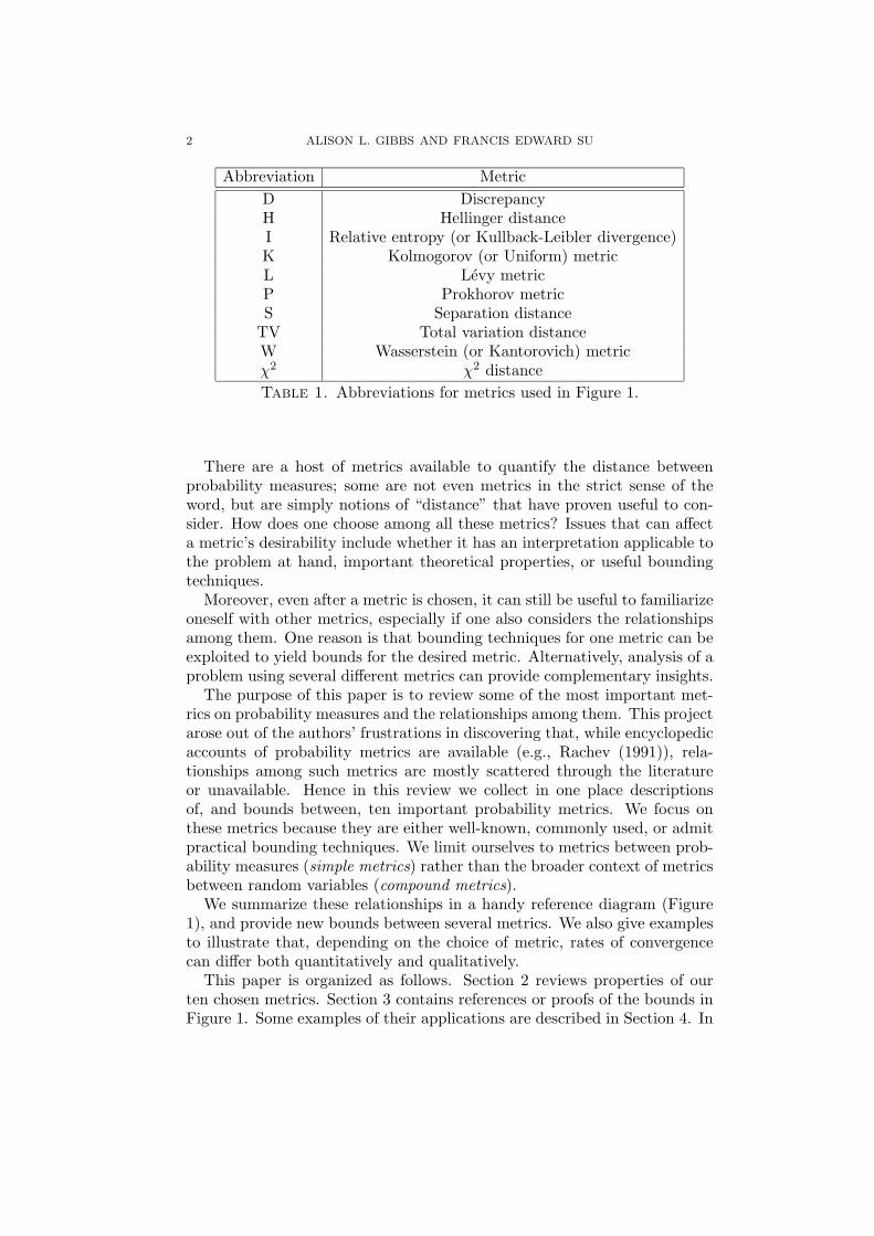
TV Total variation distanceW Wasserstein (or Kantorovich) metricχ2 χ2 distanceTable 1. Abbreviations for metrics used in Figure 1.

There are a host of metrics available to quantify the distance betweenprobability measures; some are not even metrics in the strict sense of theword, but are simply notions of “distance” that have proven useful to con-sider. How does one choose among all these metrics? Issues that can affecta metric’s desirability include whether it has an interpretation applicable tothe problem at hand, important theoretical properties, or useful boundingtechniques.

Moreover, even after a metric is chosen, it can still be useful to familiarizeoneself with other metrics, especially if one also considers the relationshipsamong them. One reason is that bounding techniques for one metric can beexploited to yield bounds for the desired metric. Alternatively, analysis of aproblem using several different metrics can provide complementary insights.

The purpose of this paper is to review some of the most important met-rics on probability measures and the relationships among them. This projectarose out of the authors’ frustrations in discovering that, while encyclopedicaccounts of probability metrics are available (e.g., Rachev (1991)), rela-tionships among such metrics are mostly scattered through the literatureor unavailable. Hence in this review we collect in one place descriptionsof, and bounds between, ten important probability metrics. We focus onthese metrics because they are either well-known, commonly used, or admitpractical bounding techniques. We limit ourselves to metrics between prob-ability measures (simple metrics) rather than the broader context of metricsbetween random variables (compound metrics).

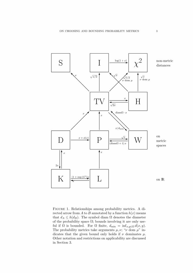
We summarize these relationships in a handy reference diagram (Figure1), and provide new bounds between several metrics. We also give examplesto illustrate that, depending on the choice of metric, rates of convergencecan differ both quantitatively and qualitatively.

This paper is organized as follows. Section 2 reviews properties of ourten chosen metrics. Section 3 contains references or proofs of the bounds inFigure 1. Some examples of their applications are described in Section 4. In

ON CHOOSING AND BOUNDING PROBABILITY METRICS 3

S

@@@@

@@I x

TV -x√

2xH

Wonmetricspaces

@@@@@@R

x/dmin @@

@@@@I diamΩ · x

-√x

(diamΩ + 1)x

√x/2

ν dom µ

@@

@@@@I√x6√

x/2

I -log(1 + x)

χ2 non-metricdistances

6√x

ν dom µ

6x

P

x

D

?2x

6x

K L on IR

6x

x

-(1 + sup |G′|)x

-x+ φ(x)

Figure 1. Relationships among probability metrics. A di-rected arrow from A toB annotated by a function h(x) meansthat dA ≤ h(dB). The symbol diam Ω denotes the diameterof the probability space Ω; bounds involving it are only use-ful if Ω is bounded. For Ω finite, dmin = infx,y∈Ω d(x, y).The probability metrics take arguments µ, ν; “ν dom µ” in-dicates that the given bound only holds if ν dominates µ.Other notation and restrictions on applicability are discussedin Section 3.

4 ALISON L. GIBBS AND FRANCIS EDWARD SU

Section 5 we give examples to show that the choice of metric can stronglyaffect both the rate and nature of the convergence.

2. Ten metrics on probability measures

Throughout this paper, let Ω denote a measurable space with σ-algebraB. Let M be the space of all probability measures on (Ω,B). We considerconvergence in M under various notions of distance, whose definitions arereviewed in this section. Some of these are not strictly metrics, but are non-negative notions of “distance” between probability distributions on Ω thathave proven useful in practice. These distances are reviewed in the ordergiven by Table 1.

In what follows, let µ, ν denote two probability measures on Ω. Let fand g denote their corresponding density functions with respect to a σ-finite dominating measure λ (for example, λ can be taken to be (µ+ ν)/2).If Ω = IR, let F , G denote their corresponding distribution functions. Whenneeded, X,Y will denote random variables on Ω such that L(X) = µ andL(Y ) = ν. If Ω is a metric space, it will be understood to be a measurablespace with the Borel σ-algebra. If Ω is a bounded metric space with metricd, let diam(Ω) = supd(x, y) : x, y ∈ Ω denote the diameter of Ω.

Discrepancy metric.1. State space: Ω any metric space.2. Definition:

dD(µ, ν) := supall closed balls B

|µ(B)− ν(B)|.

It assumes values in [0, 1].3. The discrepancy metric recognizes the metric topology of the underly-

ing space Ω. However, the discrepancy is scale-invariant: multiplyingthe metric of Ω by a positive constant does not affect the discrepancy.

4. The discrepancy metric admits Fourier bounds, which makes it usefulto study convergence of random walks on groups (Diaconis 1988, p. 34).

Hellinger distance.1. State space: Ω any measurable space.2. Definition: if f , g are densities of the measures µ, ν with respect to a

dominating measure λ,

dH(µ, ν) :=[∫

Ω(√f −√g)2 dλ

]1/2

=[2(

1−∫

Ω

√fg dλ

)]1/2

.

This definition is independent of the choice of dominating measure λ.For a countable state space Ω,

dH(µ, ν) :=

[∑ω∈Ω

(√µ(ω)−

√ν(ω)

)2]1/2

(Diaconis and Zabell 1982).

ON CHOOSING AND BOUNDING PROBABILITY METRICS 5

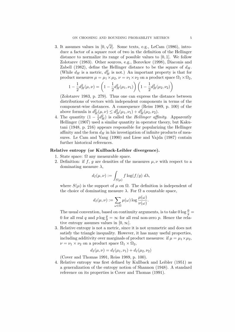
3. It assumes values in [0,√

2]. Some texts, e.g., LeCam (1986), intro-duce a factor of a square root of two in the definition of the Hellingerdistance to normalize its range of possible values to [0, 1]. We followZolotarev (1983). Other sources, e.g., Borovkov (1998), Diaconis andZabell (1982), define the Hellinger distance to be the square of dH .(While dH is a metric, d2

H is not.) An important property is that forproduct measures µ = µ1×µ2, ν = ν1×ν2 on a product space Ω1×Ω2,

1− 12d2H(µ, ν) =

(1− 1

2d2H(µ1, ν1)

)(1− 1

2d2H(µ2, ν2)

)(Zolotarev 1983, p. 279). Thus one can express the distance betweendistributions of vectors with independent components in terms of thecomponent-wise distances. A consequence (Reiss 1989, p. 100) of theabove formula is d2

H(µ, ν) ≤ d2H(µ1, ν1) + d2

H(µ2, ν2).4. The quantity (1 − 1

2d2H) is called the Hellinger affinity. Apparently

Hellinger (1907) used a similar quantity in operator theory, but Kaku-tani (1948, p. 216) appears responsible for popularizing the Hellingeraffinity and the form dH in his investigation of infinite products of mea-sures. Le Cam and Yang (1990) and Liese and Vajda (1987) containfurther historical references.

Relative entropy (or Kullback-Leibler divergence).1. State space: Ω any measurable space.2. Definition: if f , g are densities of the measures µ, ν with respect to a

dominating measure λ,

dI(µ, ν) :=∫S(µ)

f log(f/g) dλ,

where S(µ) is the support of µ on Ω. The definition is independent ofthe choice of dominating measure λ. For Ω a countable space,

dI(µ, ν) :=∑ω∈Ω

µ(ω) logµ(ω)ν(ω)

.

The usual convention, based on continuity arguments, is to take 0 log 0q =

0 for all real q and p log p0 =∞ for all real non-zero p. Hence the rela-

tive entropy assumes values in [0,∞].3. Relative entropy is not a metric, since it is not symmetric and does not

satisfy the triangle inequality. However, it has many useful properties,including additivity over marginals of product measures: if µ = µ1×µ2,ν = ν1 × ν2 on a product space Ω1 × Ω2,

dI(µ, ν) = dI(µ1, ν1) + dI(µ2, ν2)

(Cover and Thomas 1991, Reiss 1989, p. 100).4. Relative entropy was first defined by Kullback and Leibler (1951) as

a generalization of the entropy notion of Shannon (1948). A standardreference on its properties is Cover and Thomas (1991).

6 ALISON L. GIBBS AND FRANCIS EDWARD SU

Kolmogorov (or Uniform) metric.1. State space: Ω = IR.2. Definition:

dK(F,G) := supx|F (x)−G(x)|, x ∈ IR.

(Since µ, ν are measures on IR, it is customary to express the Kol-mogorov metric as a distance between their distribution functions F,G.)

3. It assumes values in [0, 1], and is invariant under all increasing one-to-one transformations of the line.

4. This metric, due to Kolmogorov (1933), is also called the uniform met-ric (Zolotarev 1983).

Levy metric.1. State space: Ω = IR.2. Definition:

dL(F,G) := infε > 0 : G(x− ε)− ε ≤ F (x) ≤ G(x+ ε) + ε,∀x ∈ IR.(Since µ, ν are measures on IR, it is customary to express the Levymetric as a distance between their distribution functions F,G.)

3. It assumes values in [0, 1]. While not easy to compute, the Levy metricdoes metrize weak convergence of measures on IR (Lukacs 1975, p. 71).It is shift invariant, but not scale invariant.

4. This metric was introduced by Levy (1925, p. 199-200).

Prokhorov (or Levy-Prokhorov) metric.1. State space: Ω any metric space.2. Definition:

dP (µ, ν) := infε > 0 : µ(B) ≤ ν(Bε) + ε for all Borel sets Bwhere Bε = x : infy∈B d(x, y) ≤ ε. It assumes values in [0, 1].

3. It is possible to show that this metric is symmetric in µ, ν. See (Huber1981, p. 27).

4. This metric was defined by Prokhorov (1956) as the analogue of theLevy metric for more general spaces. While not easy to compute, thismetric is theoretically important because it metrizes weak convergenceon any separable metric space (Huber 1981, p. 28). Moreover, dP (µ, ν)is precisely the minimum distance “in probability” between randomvariables distributed according to µ, ν. This was shown by Strassen(1965) for complete separable metric spaces and extended by Dudley(1968) to arbitrary separable metric spaces.

Separation distance.1. State space: Ω a countable space.2. Definition:

dS(µ, ν) := maxi

(1− µ(i)

ν(i)

).

ON CHOOSING AND BOUNDING PROBABILITY METRICS 7

3. It assumes values in [0, 1]. However, it not a metric.4. The separation distance was advocated by Aldous and Diaconis (1987)

to study Markov chains because it admits a useful characterization interms of strong uniform times.

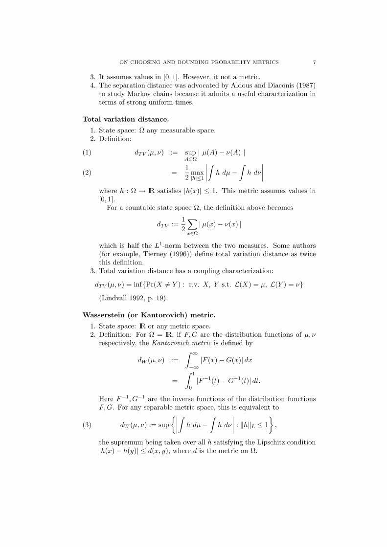
Total variation distance.

1. State space: Ω any measurable space.2. Definition:

dTV (µ, ν) := supA⊂Ω| µ(A)− ν(A) |(1)

=12

max|h|≤1

∣∣∣∣∫ h dµ−∫h dν

∣∣∣∣(2)

where h : Ω → IR satisfies |h(x)| ≤ 1. This metric assumes values in[0, 1].

For a countable state space Ω, the definition above becomes

dTV :=12

∑x∈Ω

|µ(x)− ν(x) |

which is half the L1-norm between the two measures. Some authors(for example, Tierney (1996)) define total variation distance as twicethis definition.

3. Total variation distance has a coupling characterization:

dTV (µ, ν) = infPr(X 6= Y ) : r.v. X, Y s.t. L(X) = µ, L(Y ) = ν

(Lindvall 1992, p. 19).

Wasserstein (or Kantorovich) metric.

1. State space: IR or any metric space.2. Definition: For Ω = IR, if F,G are the distribution functions of µ, ν

respectively, the Kantorovich metric is defined by

dW (µ, ν) :=∫ ∞−∞|F (x)−G(x)| dx

=∫ 1

0|F−1(t)−G−1(t)| dt.

Here F−1, G−1 are the inverse functions of the distribution functionsF,G. For any separable metric space, this is equivalent to

dW (µ, ν) := sup∣∣∣∣∫ h dµ−

∫h dν

∣∣∣∣ : ‖h‖L ≤ 1,(3)

the supremum being taken over all h satisfying the Lipschitz condition|h(x)− h(y)| ≤ d(x, y), where d is the metric on Ω.

8 ALISON L. GIBBS AND FRANCIS EDWARD SU

3. The Wasserstein metric assumes values in [0,diam(Ω)], where diam(Ω)is the diameter of the metric space (Ω, d). This metric metrizes weakconvergence on spaces of bounded diameter, as is evident from Theo-rem 2 below.

4. By the Kantorovich-Rubinstein theorem, the Kantorovich metric isequal to the Wasserstein metric:

dW (µ, ν) = infJE[d(X,Y )] : L(X) = µ,L(Y ) = ν,

where the infimum is taken over all joint distributions J with marginalsµ, ν. See Szulga (1982, Theorem 2). Dudley (1989, p. 342) traces someof the history of these metrics.

χ2-distance.

1. State space: Ω any measurable space.2. Definition: if f , g are densities of the measures µ, ν with respect to a

dominating measure λ, and S(µ), S(ν) are their supports on Ω,

dχ2(µ, ν) :=∫S(µ)∪S(ν)

(f − g)2

gdλ.

This definition is independent of the choice of dominating measure λ.This metric assumes values in [0,∞]. For a countable space Ω thisreduces to:

dχ2(µ, ν) :=∑

ω∈S(µ)∪S(ν)

(µ(ω)− ν(ω))2

ν(ω).

This distance is not symmetric in µ and ν; beware that the order ofthe arguments varies from author to author. We follow Csiszar (1967)and Liese and Vajda (1987) because of the remarks following equation(4) below and the natural order of arguments suggested by inequalities(10) and (11). Reiss (1989, p. 98) takes the opposite convention as wellas defining the χ2-distance as the square root of the above expression.

3. The χ2-distance is not symmetric, and therefore not a metric. How-ever, like the Hellinger distance and relative entropy, the χ2-distancebetween product measures can be bounded in terms of the distancesbetween their marginals. See Reiss (1989, p. 100).

4. The χ2-distance has origins in mathematical statistics dating back toPearson. See Liese and Vajda (1987, p. 51) for some history.

We remark that several distance notions in this section are instances of afamily of distances known as f-divergences (Csiszar 1967). For any convexfunction f , one may define

df (µ, ν) =∑ω

ν(ω)f(µ(ω)ν(ω)

).(4)

ON CHOOSING AND BOUNDING PROBABILITY METRICS 9

Then choosing f(x) = (x − 1)2 yields dχ2 , f(x) = x log x yields dI , f(x) =|x − 1|/2 yields dTV , and f(x) = (

√x − 1)2 yields d2

H . The family of f -divergences are studied in detail in Liese and Vajda (1987).

3. Some Relationships Among Probability Metrics

In this section we describe in detail the relationships illustrated in Fig-ure 1. We give references for relationships known to appear elsewhere, andprove several new bounds which we state as theorems. In choosing the orderof presentation, we loosely follow the diagram from bottom to top.

At the end of this section, we summarize in Theorem 6 what is knownabout how these metrics relate to weak convergence of measures.

The Kolmogorov and Levy metrics on IR. For probability measuresµ, ν on IR with distribution functions F,G,

dL(F,G) ≤ dK(F,G).

See Huber (1981, p. 34). Petrov (1995, p. 43) notes that if G(x) (i.e., ν) isabsolutely continuous (with respect to Lebesgue measure), then

dK(F,G) ≤(

1 + supx|G′(x)|

)dL(F,G).

The Discrepancy and Kolmogorov metrics on IR. It is evident thatfor probability measures on IR,

dK ≤ dD ≤ 2 dK .(5)

This follows from the regularity of Borel sets in IR and expressing closedintervals in IR as difference of rays.

The Prokhorov and Levy metrics on IR. For probability measures onIR,

dL ≤ dP .See Huber (1981, p. 34).

The Prokhorov and Discrepancy metrics. The following theorem showshow discrepancy may be bounded by the Prokhorov metric by finding a suit-able right-continuous function φ. For bounded Ω, φ(ε) gives an upper boundon the additional ν-measure of the extended ball Bε over the ball B, whereBε = x : infy∈B d(x, y) ≤ ε. Note that this theorem also gives an upperbound for dK through (5) above.

Theorem 1. Let Ω be any metric space, and let ν be any probability measuresatisfying

ν(Bε) ≤ ν(B) + φ(ε)for all balls B and complements of balls B and some right-continuous func-tion φ. Then for any other probability measure µ, if dP (µ, ν) = x, thendD(µ, ν) ≤ x+ φ(x).

10 ALISON L. GIBBS AND FRANCIS EDWARD SU

As an example, on the circle or line, if ν = U is the uniform distribution,then φ(x) = 2x and hence

dD(µ,U) ≤ 3 dP (µ,U).

Proof. For µ, ν as above,

µ(B)− ν(Bx) ≥ µ(B)− ν(B)− φ(x).

And if dP (µ, ν) = x, then µ(B)− ν(Bx) ≤ x for all x > x and all Borel setsB. Combining with the above inequality, we see that

µ(B)− ν(B)− φ(x) ≤ x.By taking the supremum over B which are balls or complements of balls,obtain

supB

(µ(B)− ν(B)) ≤ x+ φ(x).

The same result may be obtained for ν(B) − µ(B) by noting that ν(B) −µ(B) = µ(Bc)− ν(Bc) which, after taking the supremum over B which areballs or complements of balls, obtain

supB

(ν(B)− µ(B)) = supBc

(µ(Bc)− ν(Bc)) ≤ x+ φ(x)

as before. Since the supremum over balls and complements of balls willbe larger than the supremum over balls, if dP (µ, ν) = x, then dD(µ, ν) ≤x+φ(x) for all x > x. For right-continuous φ, the theorem follows by takingthe limit as x decreases to x.

The Prokhorov and Wasserstein metrics. Huber (1981, p. 33) showsthat

(dP )2 ≤ dW ≤ 2 dPfor probability measures on a complete separable metric space whose metricd is bounded by 1. More generally, we show the following:

Theorem 2. The Wasserstein and Prokhorov metrics satisfy

(dP )2 ≤ dW ≤ (diam(Ω) + 1) dP

where diam(Ω) = supd(x, y) : x, y ∈ Ω.

Proof. For any joint distribution J on random variables X,Y ,

EJ [d(X,Y )] ≤ ε · Pr(d(X,Y ) ≤ ε) + diam(Ω) · Pr(d(X,Y ) > ε)= ε+ (diam(Ω)− ε) · Pr(d(X,Y ) > ε)

If dP (µ, ν) ≤ ε, we can choose a coupling so that Pr(d(X,Y ) > ε) is boundedby ε (Huber 1981, p. 27). Thus

EJ [d(X,Y )] ≤ ε+ (diam(Ω)− ε)ε ≤ (diam(Ω) + 1)ε.

Taking the infimum of both sides over all couplings, we obtain

dW ≤ (diam(Ω) + 1)dP .

ON CHOOSING AND BOUNDING PROBABILITY METRICS 11

To bound Prokhorov by Wasserstein, use Markov’s inequality and chooseε such that dW (µ, ν) = ε2. Then

Pr(d(X,Y ) > ε) ≤ 1εEJ [d(X,Y )] ≤ ε

where J is any joint distribution on X,Y . By Strassen’s theorem (Huber1981, Theorem 3.7), Pr(d(X,Y ) > ε) ≤ ε is equivalent to µ(B) ≤ ν(Bε) + εfor all Borel sets B, giving d2

P ≤ dW .

No such upper bound on dW holds if Ω is not bounded. Dudley (1989,p. 330) cites the following example on IR. Let δx denote the delta measureat x. The measures Pn := ((n− 1)δ0 + δn)/n converge to P := δ0 under theProkhorov metric, but dW (Pn, P ) = 1 for all n. Thus Wasserstein metricmetrizes weak convergence only on state spaces of bounded diameter.

The Wasserstein and Discrepancy metrics. The following bound canbe recovered using the bounds through total variation (and is therefore notincluded on Figure 1), but we include this direct proof for completeness.

Theorem 3. If Ω is finite,

dmin · dD ≤ dWwhere dmin = minx 6=y d(x, y) over distinct pairs of points in Ω.

Proof. In the equivalent form of the Wasserstein metric, Equation (3), take

h(x) =dmin for x in B0 otherwise

for B any closed ball. h(x) satisfies the Lipschitz condition. Then

dmin · |µ(B)− ν(B)| =∣∣∣∣∫

Ωh dµ−

∫Ωh dν

∣∣∣∣≤ dW (µ, ν)

and takingB to be the ball that maximizes |µ(B)−ν(B)| gives the result.

On continuous spaces, it is possible for dW to converge to 0 while dDremains at 1. For example, take delta measures δε converging on δ0.

The Total Variation and Discrepancy metrics. It is clear that

dD ≤ dTV(6)

since total variation is the supremum over a larger class of sets than discrep-ancy.

No expression of the reverse type can hold since the total variation dis-tance between a discrete and continuous distribution is 1 while the discrep-ancy may be very small. Further examples are discussed in Section 5.

The Total Variation and Prokhorov metrics. Huber (1981, p. 34)proves the following bound for probabilities on metric spaces:

dP ≤ dTV .

12 ALISON L. GIBBS AND FRANCIS EDWARD SU

The Wasserstein and Total Variation metrics.

Theorem 4. The Wasserstein metric and the total variation distance sat-isfy the following relation:

dW ≤ diam(Ω) · dTVwhere diam(Ω) = supd(x, y) : x, y ∈ Ω. If Ω is a finite set, there is abound the other way. If dmin = minx6=y d(x, y) over distinct pairs of pointsin Ω, then

dmin · dTV ≤ dW .(7)

Note that on an infinite set no such relation of the second type can occurbecause dW may converge to 0 while dTV remains fixed at 1. (minx 6=y d(x, y)could be 0 on an infinite set.)

Proof. The first inequality follows from the coupling characterizations ofWasserstein and total variation by taking the infimum of the expected valueover all possible joint distributions of both sides of:

d(X,Y ) ≤ 1X 6=Y · diam(Ω).

The reverse inequality follows similarly from:

d(X,Y ) ≥ 1X 6=Y ·mina 6=b

d(a, b).

The Hellinger and Total Variation metrics.

(dH)2

2≤ dTV ≤ dH .(8)

See LeCam (1969, p. 35).

The Separation distance and Total Variation. It is easy to show (see,e.g., Aldous and Diaconis (1987, p. 71)) that

dTV ≤ dS .(9)

As Aldous and Diaconis note, there is no general reverse inequality, sinceif µ is uniform on 1, 2, ..., n and ν is uniform on 1, 2, ..., n − 1 thendTV (µ, ν) = 1/n but dS(µ, ν) = 1.

Relative Entropy and Total Variation. For countable state spaces Ω,

2 (dTV )2 ≤ dI .This inequality is due to Kullback (1967). Some small refinements are pos-sible where the left side of the inequality is replaced with a polynomial indTV with more terms; see Mathai and Rathie (1975, p. 110-112).

Relative Entropy and the Hellinger distance.

(dH)2 ≤ dI .See Reiss (1989, p. 99).

ON CHOOSING AND BOUNDING PROBABILITY METRICS 13

The χ2-distance and Hellinger distance.

dH(µ, ν) ≤√

2( dχ2(µ, ν))1/4.

See Reiss (1989, p. 99), who also shows that if the measure µ is dominatedby ν, then the above inequality can be strengthened:

dH(µ, ν) ≤ (dχ2(µ, ν))1/2.

The χ2-distance and Total Variation. For a countable state space Ω,

dTV (µ, ν) =12

∑ω∈Ω

|µ(ω)− ν(ω)|√ν(ω)

√ν(ω) ≤ 1

2

√dχ2(µ, ν)

where the inequality follows from Cauchy-Schwarz. On a continuous statespace, if µ is dominated by ν the same relationship holds; see Reiss (1989,p. 99).

The χ2-distance and Relative Entropy.

Theorem 5. The relative entropy dI and the χ2-distance dχ2 satisfy

dI(µ, ν) ≤ log[1 + dχ2(µ, ν)

].(10)

In particular, dI(µ, ν) ≤ dχ2(µ, ν).

Proof. Since log is a concave function, Jensen’s inequality yields

dI(µ, ν) ≤ log(∫

Ω(f/g) f dλ

)≤ log

(1 + dχ2(µ, ν)

)≤ dχ2(µ, ν),

where the second inequality is obtained by noting that∫Ω

(f − g)2

gdλ =

∫Ω

(f2

g− 2f + g

)dλ =

∫Ω

f2

gdλ− 1.

Diaconis and Saloff-Coste (1996, p. 710) derive the following alternate upperbound for the relative entropy in terms of both the χ2 and total variationdistances.

dI(µ, ν) ≤ dTV (µ, ν) +12dχ2(µ, ν).(11)

Weak convergence. In addition to using Figure 1 to recall specific bounds,our diagram there can also be used to discern relationships between topolo-gies on the space of measures. For instance, we can see from the mutualarrows between the total variation and Hellinger metrics that they generateequivalent topologies. Other mutual arrows on the diagram indicate similarrelationships, subject to the restrictions given on those bounds.

Moreover, since we know that the Prokhorov and Levy metrics bothmetrize weak convergence, we can also tell which other metrics metrize weakconvergence on which spaces, which we summarize in the following theorem:

14 ALISON L. GIBBS AND FRANCIS EDWARD SU

Theorem 6. For measures on IR, the Levy metric metrizes weak conver-gence. Convergence under the discrepancy and Kolmogorov metrics implyweak convergence (via the Levy metric). Furthermore, these metrics metrizeweak convergence µn → ν if the limiting metric ν is absolutely continuouswith respect to Lebesgue measure on IR.

For measures on a measurable space Ω, the Prokhorov metric metrizesweak convergence. Convergence under the Wasserstein metric implies weakconvergence.

Furthermore, if Ω is bounded, the Wasserstein metric metrizes weak con-vergence (via the Prokhorov metric), and convergence under any of the fol-lowing metrics implies weak convergence: total variation, Hellinger, separa-tion, relative entropy, and the χ2-distance.

If Ω is both bounded and finite, the total variation and Hellinger metricsboth metrize weak convergence.

This follows from chasing the diagram in Figure 1, noting the existenceof mutual bounds of the Levy and Prokhorov metrics with other metrics(using the results surveyed in this section) and reviewing conditions underwhich they apply.

4. Some Applications of Metrics and Metric Relationships

We describe some of the applications of these metrics in order to givethe reader a feel for how they have been used, and describe how some au-thors have exploited metric relationships to obtain bounds for one metricvia another.

The notion of weak convergence of measures is an important concept inboth statistics and probability. For instance, when considering a statistic Tthat is a functional of an empirical distribution F , the “robustness” of thestatistic under small deviations of F corresponds to the continuity of T withrespect to the weak topology on the space of measures. See Huber (1981).The Levy and Prokhorov metrics (and Wasserstein metric on a boundedstate space) provide quantitative ways of metrizing this topology.

However, other distances that do not metrize this topology can still beuseful for other reasons. The total variation distance is one of the most com-monly used probability metrics, because it admits natural interpretations aswell as useful bounding techniques. For instance, in (1), if A is any event,then total variation can be interpreted as an upper bound on the differenceof probabilities that the event occurs under two measures. In Bayesian sta-tistics, the error in an expected loss function due to the approximation ofone measure by another is given (for bounded loss functions) by the totalvariation distance through its representation in equation (2).

In extending theorems on the ergodic behavior of Markov chains on dis-crete state spaces to general measurable spaces, the total variation norm is

ON CHOOSING AND BOUNDING PROBABILITY METRICS 15

used in a number of results (Orey 1971, Nummelin 1984). More recently, to-tal variation has found applications in bounding rates of convergence of ran-dom walks on groups (e.g., Diaconis (1988), Rosenthal (1995)) and Markovchain Monte Carlo algorithms (e.g., Tierney (1994), Gilks, Richardson andSpiegelhalter (1996)). Much of the success in obtaining rates of convergencein these settings is a result of the coupling characterization of the totalvariation distance, as well as Fourier bounds.

Gibbs (2000) considers a Markov chain Monte Carlo algorithm whichconverges in total variation distance, but for which coupling bounds aredifficult to apply since the state space is continuous and one must wait forrandom variables to couple exactly. The Wasserstein metric has a couplingcharacterization that depends on the distance between two random variables,so one may instead consider only the time required for the random variablesto couple to within ε, a fact exploited by Gibbs. For a related example witha discrete state space, Gibbs uses the bound (7) to obtain total variationbounds.

Like the total variation property (2), the Wasserstein metric also repre-sents the error in the expected value of a certain class of functions due tothe approximation of one measure by another, as in (3), which is of interestin applications in Bayesian statistics. The fact that the Wasserstein metricis a minimal distance of two random variables with fixed distributions hasalso led to its use in the study of distributions with fixed marginals (e.g.,Ruschendorf, Schweizer and Taylor (1996)).

Because the separation distance has a characterization in terms of stronguniform times (like the coupling relationship for total variation), conver-gence of a Markov chain under the separation distance may be studied byconstructing a strong uniform time for the chain and estimating the proba-bility in the tail of its distribution. See Aldous and Diaconis (1987) for suchexamples; they also exploit inequality (9) to obtain upper bounds on thetotal variation.

Similarly, total variation lower bounds may be obtained via (6) and lowerbounds on the discrepancy metric. A version of this metric is popular amongnumber theorists to study uniform distribution of sequences (Kuipers andNiederreiter 1974); Diaconis (1988) suggested its use to study random walkson groups. Su (1998) uses the discrepancy metric to bound the convergencetime of a random walk on the circle generated by a single irrational rotation.This walk converges weakly, but not in total variation distance because itsn-th step probability distribution is finitely supported but its limiting mea-sure is continuous (in fact, uniform). While the Prokhorov metric metrizesweak convergence, it is not easy to bound. On the other hand, for thiswalk, discrepancy convergence implies weak convergence when the limitingmeasure is uniform; and Fourier techniques for discrepancy allow the calcu-lation of quantitative bounds. The discrepancy metric can be used similarlyto study random walks on other homogeneous spaces, e.g., Su (2001).

16 ALISON L. GIBBS AND FRANCIS EDWARD SU

Other metrics are useful because of their special properties. For instance,the Hellinger distance is convenient when working with convergence of prod-uct measures because it factors nicely in terms of the convergence of the com-ponents. Reiss (1989) uses this fact and the relationships (8) between theHellinger and total variation distances to obtain total variation bounds. TheHellinger distance is also used in the theory of asymptotic efficiency (e.g.,see LeCam (1986)) and minimum Hellinger distance estimation (e.g., seeLindsay (1994)). It is used throughout Ibragmiov and Has’minskii (1981) toquantify the rate of convergence of sequences of consistent estimators to theirparameter. Kakutani (1948) gives a criterion (now known as the Kakutanialternative) using the Hellinger affinity to determine when infinite productsof equivalent measures are equivalent; this has applications to stochasticprocesses and can be used to show the consistency of the likelihood-ratiotest. See Jacod and Shiryaev (1987), Williams (1991) for applications.

Diaconis and Saloff-Coste (1996) use log-Sobolev techniques to bound theχ2 convergence of Markov chains to their limiting distributions, noting thatthese also give total variation and entropy bounds. The χ2-distance bearsits name because in the discrete case it is the well-known χ2 statistic used,for example, in the classic goodness-of-fit test, e.g., see Borovkov (1998,p. 184). Similarly, the Kolmogorov metric between a distribution functionand its empirical estimate is used as the test statistic in the Kolmogorov-Smirnov goodness-of-fit test, e.g., see Lehmann (1994, p. 336).

Relative entropy is widely used because it is a quantity that arises natu-rally, especially in information theory (Cover and Thomas 1991). Statisticalapplications include proving central limit theorems (Linnik 1959, Barron1986) and evaluating the loss when using a maximum likelihood versus aBayes density estimate (Hartigan 1998). In the testing of an empirical dis-tribution against an alternative, Borovkov (1998, p. 256) gives the relation-ship of the asymptotic behaviour of the Type II error to the relative entropybetween the empirical and alternative distributions. In Bayesian statistics,Bernardo and Smith (1994, p. 75) suggest that relative entropy is the nat-ural measure for the lack of fit of an approximation of a distribution whenpreferences are described by a logarithmic score function.

Up to a constant, the asymptotic behaviour of relative entropy, the Hellinger,and the χ2-distance are identical when the ratio of the density functions isnear 1 (Borovkov 1998, p. 178). These three distances are used extensivelyin parametric families of distributions to quantify the distance between mea-sures from the same family indexed by different parameters. Borovkov (1998,pp. 180-181) shows how these distances are related to the Fisher informationin the limit as the difference in the parameters goes to zero.

5. Rates of Convergence that Depend on the Metric

We now illustrate the ways in which the choice of metric can affect rates ofconvergence in one context: the convergence of a random walk to its limitingdistribution. Such examples point to the need for practitioners to choose

ON CHOOSING AND BOUNDING PROBABILITY METRICS 17

a metric carefully when measuring convergence, paying attention to thatmetric’s qualitative and quantitative features. We give several examples ofrandom walks whose qualitative convergence behavior depend strongly onthe metric chosen, and suggest reasons for this phenomenon.

As a first basic fact, it is possible for convergence to occur in one metricbut not another. An elementary example is the convergence of a stan-dardized Binomial (n, p) random variable with distribution µn which con-verges to the standard normal distribution, ν, as n → ∞. For all n < ∞,dTV (µn, ν) = 1, while dD(µn, ν) → 0 as n → ∞. In the random walk con-text, Su (1998) shows that a random walk on the circle generated by anirrational rotation converges in discrepancy, but not total variation. Thelatter fact follows because the n-th step probability distribution is finitelysupported, and remains total variation distance 1 away from its continuouslimiting distribution.

However, more interesting behavior can arise. Below, we cite a familyof random walks on a product space, indexed by some parameter, whichnot only converges under each of total variation, relative entropy, and theχ2-distance, but exhibits different rates of convergence as a function of theparameter.

We then cite another example of a family of walks that not only hasdifferent convergence rates under two different metrics, but also exhibitsqualitatively different convergence behavior. This family exhibits a cutoffphenomenon under the first metric but only exponential decay under thesecond.

Example: convergence rates that depend on the metric. The follow-ing family of random walks show that convergence rates in total variation,relative entropy, and χ2-distance may differ. Recall that a family of randomwalks, indexed by some parameter n, is said to converge in f(n) steps us-ing some metric/distance if that metric/distance can be uniformly boundedfrom above after f(n) steps and is uniformly bounded away from zero beforef(n) steps.

Let G = Z mod g, a finite group with g elements. Then Gn is the setof all n-tuples of elements from G. Consider the following continuous-timerandom walk on Gn: start at (0, 0, ..., 0) and according to a Poisson processrunning at rate 1, pick a coordinate uniformly at random and replace thatcoordinate by a uniformly chosen element from G. (Thus each coordinate isan independent Poisson process running at rate 1

n .)Su (1995) proves that if g grows with n exponentially according to g = 2n,

then the random walk on Gn described above converges in 2n log n stepsunder the relative entropy distance, and n2 log 2 steps under the χ2-distance.However, it converges in at most n log n steps under total variation.

In this example, the relative entropy and χ2-distance are calculated byusing properties of these metrics, while the total variation upper bound in

18 ALISON L. GIBBS AND FRANCIS EDWARD SU

this example is, in fact, calculated via its metric relationship (9) with theseparation distance.

Why does the difference in rates of convergence occur? This is due to thefact that total variation distance, unlike relative entropy or the χ2-distance,is insensitive to big or small elementwise differences when the total of thosedifferences remains the same. For instance, consider the follow measuresµ, ν on Z10. Let

µ(i) =

0.6 if i = 00.1 if i = 1, 2, 3, 40 else

ν(i) =

0.2 if i = 0, 1, 2, 3, 40 else .

Let U be the uniform distribution on Z10. In this example dI(µ,U) ≈1.075 and dI(ν, U) = 0.693, but the total variation distances are the same:dTV (µ,U) = dTV (ν, U) = 0.5. This is true because we could redistributemass among the points on which µ exceeded ν without affecting the totalvariation distance.

Thus it is possible for an unbalanced measure (with large elementwisedifferences from uniform) to have the same total variation distance as amore balanced measure. The random walk on the product space has anatural feature which rewards total variation distance but hinders relativeentropy— the randomization in each coordinate drops the variation distancequickly, but balancing the measure might take longer.

Example: qualitatively different convergence behavior. Chung, Di-aconis and Graham (1987) study a family of walks that exhibits a cutoffphenomenon under total variation; the total variation distance stays near 1but drops off sharply and steeply to zero after a certain cutoff point. Thefamily of random walks is on the integers mod p where p is an odd num-ber, with a randomness multiplier: the process is given by X0 = 0 andXn = 2Xn−1 + εn (mod p) where the εi are i.i.d. taking values 0, ±1 eachwith probability 1/3. The stationary distribution for this process is uni-form. Using Fourier analysis, Chung et al. (1987) show for the family ofwalks when p = 2t − 1 that O(log2 p log log2 p) steps are sufficient and nec-essary for total variation convergence, for t a positive integer. There is, infact, a cutoff phenomenon.

However, as proven in Su (1995, pp. 29-31), O(log p) steps are sufficient forconvergence in discrepancy. Moreover, the convergence is qualitatively dif-ferent from total variation, because there is no cutoff in discrepancy. Rather,there is only exponential decay.

Again, analysis under these two metrics sheds some light on what thewalk is doing. For p = 2t − 1, the “doubling” nature of the process keepsthe walk supported very near powers of 2. The discrepancy metric, whichaccounts for the topology of the space, falls very quickly because the walkhas spread itself out even though it is supported on a small set of values.However, the total variation does not “see” this spreading; it only falls whenthe support of the walk is large enough.

ON CHOOSING AND BOUNDING PROBABILITY METRICS 19

Thus, the difference in rates of convergence sheds some light on the natureof the random walk as well as the metrics themselves.

References

Aldous, D. and Diaconis, P. (1987). Strong uniform times and finite random walks, Adv.in Appl. Math. 8: 69–97.

Barron, A. (1986). Entropy and central limit theorem, Ann. Probab. 14: 336–42.Bernardo, J. M. and Smith, A. F. M. (1994). Bayesian Theory, John Wiley & Sons,

Chichester, England.Borovkov, A. A. (1998). Mathematical Statistics, Gordon and Breach Science Publishers,

Amsterdam. Translated from the Russian by A. Moullagaliev and revised by theauthor.

Chung, F., Diaconis, P. and Graham, R. L. (1987). Random walks arising in randomnumber generation, Ann. Probab. 15: 1148–1165.

Cover, T. M. and Thomas, J. A. (1991). Elements of Information Theory, John Wiley &Sons Inc., New York. A Wiley-Interscience Publication.

Csiszar, I. (1967). Information type measures of difference of probability distributions andindirect observations, Studia Sci. Math. Hungar. 2: 299–318.

Diaconis, P. (1988). Group Representations in Probability and Statistics, Institute of Math-ematical Statistics, Hayward, CA.

Diaconis, P. and Saloff-Coste, L. (1996). Logarithmic Sobolev inequalities for finite Markovchains, Ann. Appl. Probab. 6(3): 695–750.

Diaconis, P. and Zabell, S. L. (1982). Updating subjective probability, J. Amer. Statist.Assoc. 77: 822–830.

Dudley, R. M. (1968). Distances of probability measures and random variables, Ann. Math.Statist. 39: 1563–1572.

Dudley, R. M. (1989). Real Analysis and Probability, Wadsworth & Brooks/Cole, Belmont,CA.

Gibbs, A. L. (2000). Convergence of Markov Chain Monte Carlo Algorithms with Appli-cations to Image Restoration, PhD thesis, University of Toronto.

Gilks, W. R., Richardson, S. and Spiegelhalter, D. J. (eds) (1996). Markov Chain MonteCarlo in Practice, Chapman and Hall, London.

Hartigan, J. A. (1998). The maximum likelihood prior, Ann. Statist. 26: 2083–103.Hellinger, E. (1907). Die Orthogonalinvarianten quadratischer Formen von unendlich vie-

len Variablen, Dissertation, Gottingen.Huber, P. J. (1981). Robust Statistics, John Wiley & Sons, New York.Ibragmiov, I. A. and Has’minskii, R. Z. (1981). Statistical Estimation: Asymptotic Theory,

Springer-Verlag, New York.Jacod, J. and Shiryaev, A. N. (1987). Limit Theorems for Stochastic Processes, Springer-

Verlag, Berlin.Kakutani, S. (1948). On equivalence of infinite product measures, Ann. of Math. (2)

49: 214–224.Kolmogorov, A. N. (1933). Sulla determinazione empirica di una legge di distribuzione,

Giornale dell’Istituto Italiano degli Attuari 4: 83–91.Kuipers, L. and Niederreiter, H. (1974). Uniform Distribution of Sequences, Wiley-

Interscience [John Wiley & Sons], New York. Pure and Applied Mathematics.Kullback, S. (1967). A lower bound for discrimination in terms of variation, IEEE Trans.

Inform. Theory 4: 126–127.Kullback, S. and Leibler, R. A. (1951). On information and sufficiency, Ann. Math. Sta-

tistics 22: 79–86.Le Cam, L. and Yang, G. L. (1990). Asymptotics in Statistics: Some Basic Concepts,

Springer-Verlag, New York.

20 ALISON L. GIBBS AND FRANCIS EDWARD SU

LeCam, L. M. (1969). Theorie Asymptotique de la Decision Statistique, Les Presses del’Universite de Montreal, Montreal.

LeCam, L. M. (1986). Asymptotic Methods in Statistical Decision Theory, Springer-Verlag,New York.

Lehmann, E. L. (1994). Testing Statistical Hypotheses, 2nd edn, Chapman & Hall, NewYork.

Levy, P. (1925). Calcul des Probabilities, Gauthiers-Villars, Paris.Liese, F. and Vajda, I. (1987). Convex Statistical Distances, B.G. Teubner Verlagsge-

sellschaft, Leipzig.Lindsay, B. G. (1994). Efficiency versus robustness: The case for minimum Hellinger

distance and related methods, Ann. Statist. 22: 1081–1114.Lindvall, T. (1992). Lectures on the Coupling Method, John Wiley & Sons, New York.Linnik, Y. V. (1959). An information-theoretic proof of the central limit theorem with the

Lindeberg condition, Theory Probab. Appl. 4: 288–99.Lukacs, E. (1975). Stochastic convergence, second edn, Academic Press [Harcourt Brace

Jovanovich Publishers], New York. Probability and Mathematical Statistics, Vol. 30.Mathai, A. M. and Rathie, P. N. (1975). Basic Concepts in Information Theory, Wiley

Eastern, New Delhi.Nummelin, E. (1984). General Irreducible Markov Chains and Nonnegative Operators,

Cambridge University Press, Cambridge.Orey, S. (1971). Lecture Notes on Limit Theorems for Markov Chain Transition Proba-

bilities, Van Nostrand Reinhold Co., London. Van Nostrand Reinhold MathematicalStudies, No. 34.

Petrov, V. V. (1995). Limit theorems of probability theory, The Clarendon Press OxfordUniversity Press, New York. Sequences of independent random variables, OxfordScience Publications.

Prokhorov, Y. V. (1956). Convergence of random processes and limit theorems in proba-bility theory, Teor. Veroyatnost. i Primenen. 1: 177–238. English translation: TheoryProbab. Appl. 1 (1956), 157-214.

Rachev, S. T. (1991). Probability Metrics and the Stability of Stochastic Models, JohnWiley & Sons, Chichester, New York.

Reiss, R.-D. (1989). Approximate Distributions of Order Statistics, Springer-Verlag, NewYork.

Rosenthal, J. S. (1995). Convergence rates of Markov chains, SIAM Rev. 37: 387–405.Ruschendorf, L., Schweizer, B. and Taylor, M. D. (eds) (1996). Distributions with Fixed

Marginals and Related Topics, Vol. 28 of Lecture Notes – Monograph Series, Instituteof Mathematical Statistics, Hayward, California.

Shannon, C. E. (1948). A mathematical theory of communication, Bell System Tech. J.27: 379–423, 623–656.

Strassen, V. (1965). The existence of probability measures with given marginals, Ann.Math. Statist 36: 423–439.

Su, F. E. (1995). Methods for Quantifying Rates of Convergence for Random Walks onGroups, PhD thesis, Harvard University.

Su, F. E. (1998). Convergence of random walks on the circle generated by an irrationalrotation, Trans. Amer. Math. Soc. 350: 3717–3741.

Su, F. E. (2001). Discrepancy convergence for the drunkard’s walk on the sphere, Electron.J. Probab. 6: no. 2, 20 pp. (electronic).

Szulga, A. (1982). On minimal metrics in the space of random variables, Theory Probab.Appl. 27: 424–430.

Tierney, L. (1994). Markov chains for exploring posterior distributions, with discussion,Ann. Statist. 22: 1701–1762.

ON CHOOSING AND BOUNDING PROBABILITY METRICS 21

Tierney, L. (1996). Introduction to general state-space Markov chain theory, in W. R.Gilks, S. Richardson and D. J. Spiegelhalter (eds), Markov Chain Monte Carlo inPractice, Chapman and Hall, London, pp. 59–74.

Williams, D. (1991). Probability with Martingales, Cambridge University Press, Cam-bridge.

Zolotarev, V. M. (1983). Probability metrics, Theory Probab. Appl. 28: 278–302.

Department of Mathematics and Statistics, York University, 4700 Keele

Street, Toronto, Ontario, Canada, M3J 1P3

E-mail address: agibbs@mathstat.yorku.ca

Department of Mathematics, Harvey Mudd College, Claremont, CA, U.S.A.

91711

E-mail address: su@math.hmc.edu