ON DEVELOPING MACRO-DIAGNOSTICS FOREVALUATING THE FISCAL HEALTH OF THE

INDIAN STATES: THE CASE OF MADHYA PRADESH

Abhay PetheMala Lalvani

DEPARTMENT OF ECONOMICSUNIVERSITY OF MUMBAI

Dr. Vibhooti Shukla Unit in Urban Economics& Regional Development

WORKING PAPER NO. 4

On Developing Macro-Diagnostics For Evaluating TheFiscal Health Of The Indian States: The Case Of Madhya

Pradesh

Abhay Pethe and Mala Lalvani∗∗

ABSTRACT

The context of this paper is given by the parametric environmentdefined by the political reality on one hand and the process ofdecentralisation which has gained impetus post 73rd and 74th

Constitutional Amendment Acts, on the other. Keeping in viewthe process of globalisation and privatisation in the Indianeconomy it suggests a conceptual framework for developingMacro-Diagnostics for evaluating the fiscal health of the Indianstates. Specifically this paper looks at the state of MadhyaPradesh. It provides an overview of key fiscal variables and theirdynamics in recent times. It also tries to operationalise theconceptual framework by way of constructing various indices. Itthus provides an entrée – by way of providing macrobenchmarks – into the rather stiff problem of development ofMadhya Pradesh’s economy.

∗ Abhay Pethe and Mala Lalvani are faculty members in the Department of Economics, University ofMumbai. The authors wish to record their sense of appreciation for useful suggestions by Ajit Karnik. Wealso thank R.K. Mishra of ORF foundation for suggesting that we undertake this study.

1

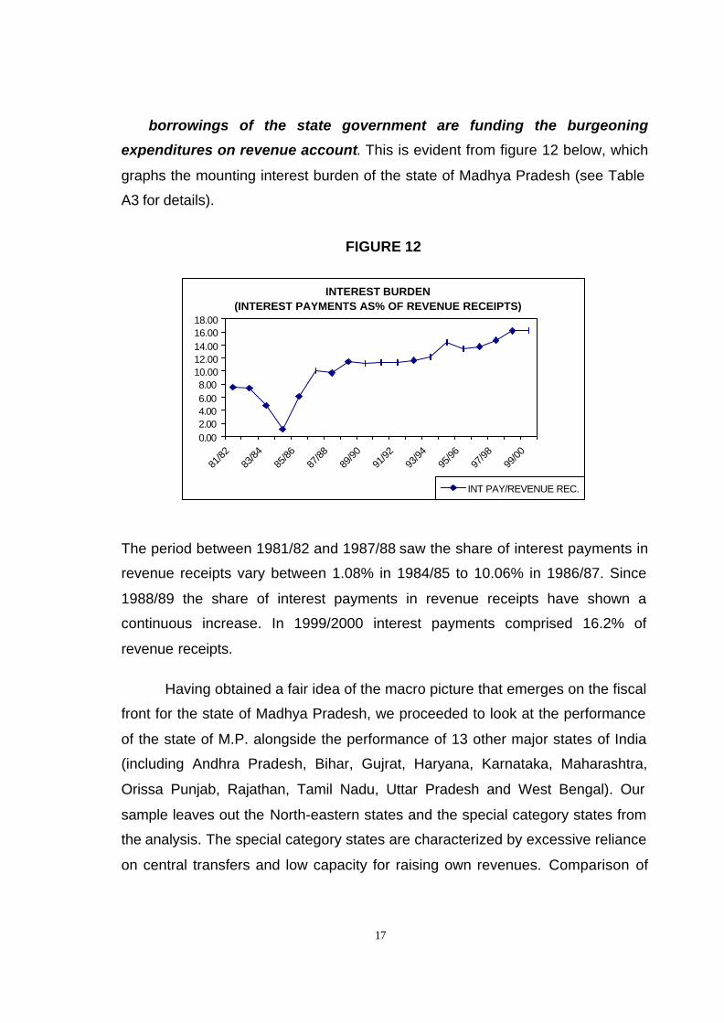
ON DEVELOPING MACRO-DIAGNOSTICS FOR EVALUATING THEFISCAL HEALTH OF THE INDIAN STATES: THE CASE OF MADHYA

PRADESH

Abhay Pethe and Mala Lalvani

1. Introduction

Indian Economy has been passing through a tumultuous phase in the last

dozen years or so. Unfolding of that eventful saga is common knowledge to all

concerned, as a part of folklore of the contemporary history of Indian Economy. It

continues to provide a point of departure for any meaningful discussion of the

Indian Economy. Globalisation and privatisation apart, the happenings in the

political sphere (especially in the realm of partisan politics) have added a new

parametric dimension to relevant reality. We are of course referring to the

strengthening of regional parties and emergence of coalition politics at all levels

of government. The states have now donned a new avatar and have become key

(sometimes, competing) players in the process of development. The recent

macroeconomic management regimen has meant that whereas on one hand

they are expected to increasingly assume newer responsibilities, on the other

they have to look after themselves when it comes to raising resources. This last

point has become an important central focus after the passage of 73rd and 74th

Constitutional Amendments. Decentralisation that was always talked about but

‘never really invited in’ has now finally, taken the centre stage. Consequently, the

political and economic aspects of governance and functional management have

come into sharp focus. No serious social scientist can afford to ignore this

backdrop whilst conducting a meaningful and fruitful discussion regarding

fostering an economically viable civil society in India.

Civil society as an item on economic and political agenda of social

thinkers has staged a dramatic return in the late twentieth century. It has been

used by social scientists in the west as well as the east and across the wide

political spectrum. It has not always meant the same thing to all of them. After all,

civil society is not a new concept. It is much older to Hegel, and entered the

2

English language usage through the Latin translation Societas Civilis, of

Aristotle’s Koinonia Politike.(Kaviraj and Khilnani, 2001). In its original sense

there was no distinction between the state and the society. Hegel was perhaps

the first to create such a bifurcation. From the point of view of developing

economy like India, we think that it is better to interpret civil society to refer to the

state and non-state initiatives for reorganisation of social life around a modern

sovereign state. The idea has to encompass all levels of governments in the vein

of political decentralisation and has to be comprehensively participative in its

connotation to encompass the NGOs and other such formal and non-formal

private sector institutions.

With the conceptual background mentioned, let us turn to the specific

concerns of our paper. The paper substantially deals with only the economic

aspects of the fiscal operations of Madhya Pradesh’s economy from a macro

view point. This is an exploratory study, trying to develop diagnostics for

evaluating a state’s fiscal health. This paper is divided into four sections including

the introduction. In the next section, we present the conceptual framework that

we will try to operationalise for attempting to develop a diagnostic for evaluating

the fiscal health of a state’s economy. In the third section we provide a backdrop

about the state of Madhya Pradesh and then report our computational results. In

the fourth and last section we conclude.

2. The Conceptual Framework

There are several macro fiscal variables available that could be looked at. It

is, however, essential to use the principle of parsimony and identify a few crucial

ones. These need to be such that the relevant data are easily available. They

must be consistently and uniformly tractable. They should thus satisfy the

theoretical tenets and not be too difficult to handle empirically. In order to

evaluate the fiscal health or performance, we need to first identify the principles

that would form the conceptual framework. Here we suggest a conceptual

framework (partly inspired by Karnik, Pethe, and Karmarkar, 2002) that is

characterised by EASE. The acronym stands for the following:

3

E for equity

A for adequacy

S for simplicity &

E for efficiency.

We will now elaborate on each of the above

Equity is a crucially important need based component. An authority that

assumes a paternal role, vis-à-vis its citizens, can ill afford to neglect this aspect.

Distributional considerations are paramount. Non-homothetic growth may be a

natural phenomenon in some cases, but has weighty objections lined against it in

the context of political economy. If the power has to go to the people and their

aspirations are to find articulation through the functioning of governments, they

have to be empowered. The need for equity is not just based on moral-ethico-

political precepts. Post Keynes and given the inter-dependant nature of a

maturing economy, it is dictated by sturdy economic sense. Unless a basic level

of development and dynamism is achieved in the rural sector, the urban sector

will find it successively more difficult to grow and develop (suffocated as it will be

by effective demand). This of course, will impact on overall economic

development of India as a whole. The huge market potential for both

consumption and producer goods (which is so very essential for a vibrant

economy) will remain a distant chimera. From the specific point of view of this

paper, equity can be broadly looked at in two ways. One, in the tax revenue that

is collected, the component that is raised by way of indirect taxes is considered

iniquitous. Two, we know that consideration of only the tax side without

considering the budget in totality is incorrect. Thus, we consider the impact on

poverty due to fiscal operations as a whole. Using these we try to operationalise

‘equity’.

Adequacy: Scarcity is omnipresent; indeed it is the raison d’être for

economics and economists. The resource gap between what is available and

4

what is ‘needed’ will be with us in the foreseeable future. This reflects what is

‘needed’ by the relevant state government. There is normally a tendency to

overestimate ones own needs (both because one really believes it and also as a

bargaining strategy, especially where hand-outs are involved). However one

needs to have some sense of the absorptive capacity of the state. Sudden

increase in funds will lead to inefficiencies in terms of consumption as well as

production use.

One way out of the difficulty is to increase the Central pool of funds to be

disbursed to a substantial extent. Given the context of the current fiscal

compression at the Central government level, one cannot realistically expect too

much via this route. The states must learn to stand up for, and help themselves.

This solution has its own limits and is beset with problems; however, there is no

readily available alternative. Efforts for closing this gap by states must be lauded

and rewarded. There are many issues that are involved here. For instance there

is the question of the extent to which sub-national governments may be allowed

to set their own taxes. It is feared that excessive latitude in this regard can create

unacceptable level of complexity and administrative burden, as well as spatial

inequities and distortions in allocation of resources. Within limits, these problems

need to be tolerated in the interest of gaining the benefits of decentralized

government. There is the other issue of changing regulatory practices in order to

allow a greater access to the credit markets for the State governments. Which of

these is the better option is a moot question answerable only in terms of actual

empirical evidence. Indeed, rather than a clear option, this involves a selection of

a proper mix of these and similar such possibilities. The need to try out

innovative experiments however is beyond doubt. One of the important lessons

that can be learnt from evidence elsewhere is that it is better if commercial

principles are followed and the state governments have to compete for capital

with other borrowing agencies in the interest of efficient utilization of resources.

In this paper, we look at the different resource gaps for the state of Madhya

Pradesh and construct an index thereof.

5

Simplicity: This characteristic is very important as it serves – at least

partially –the twin purposes of transparency and accountability. Checking and

replicating the diagnostics/ indices as given by our formulation should be easily

possible in the public domain. Ad-hocism in setting the diagnostics has the great

defect that it makes even discussion and criticism difficult. Also, there is a loss of

credibility and all kinds of suspicions about motivation begins to surface, which is

counter productive. The word “simple” used above is being used as an antonym

of complex. Of course, given the multitude of factors (e.g.,data availability) that

need to be considered, complications are bound to arise. Computational

transparency also lends itself to constructive discussion, in that, it is possible to

undertake the exercise of scenario building and simulation (not done in this

paper), and present it to the ultimate policy maker.

Efficiency: This is really a corner stone of our conceptual framework. In

the present context of the Indian economy, whence we are in the process of

making changes in the way we conduct our macro-management affairs, there

can be no doubt about the importance of having incentive compatible systems in

place. As economists, we would push very hard for this component to be the

most important one in the scheme of things. However, political feasibility as well

as adequacy requirements restrain us from going too far. Incentive compatible

system implies that every effort reflected in performance gets a reward and every

slide on efficiency front is penalised. Also, there is a static and a dynamic

component to this criterion. For example, if a state is well off in its current

performance terms, this will be a plus. Further, if its performance involves a

switch in regime (i.e., from being relatively better, a state becomes absolutely

better off; illustratively, this will happen when its small deficit changes into

surplus), once again a few bonus points may be given to the State. Alternatively,

a state may be badly off but if it shows improvement (a return of the prodigal to

the fold!) it would be entitled to a bonus. Logically, efficiency as a criterion can

conflict with some of the other components in our conceptual frame. This is a

standard problem of a multi-objective decision function. Thus, it is conceptually

necessary to set up the decision function in an add-on fashion rather than in a

6

single simple formula. Of course, ultimately the whole exercise can be

consolidated and hence a single Index is implied, even by this approach (not

attempted in this paper). We have tried to operationalise this criterion by using

several proxies as will be apparent in the next section, where we focus on

Madhya Pradesh.

3. Madhya Pradesh

The state of Madhya Pradesh (M.P) is the second largest state in India

covering a geographical area of 308 thousand sq. kms. It has an administrative

setup comprising 9 divisions, 45 districts, 370 towns/cities and 55841 villages.

The 2001 census provisionally puts the population of M.P. at 603.85 lakhs and a

population density of 196 persons per sq. km., which is way below the all India

figure of 324. The literacy rate of M.P. as registered in the 2001 census is

64.11%. This is a significant improvement from 52.2% recorded in the 1991

census. The net state domestic product of M.P in real terms (at 93/94 prices)

stood at Rs. 45744.12 crores in 1999/2000 as compared to Rs. 34357.69 crores

in 1994/95. The per capita income in real terms has risen from Rs. 6569 in

1993/94 to Rs. 7846 in 1999/2000. An overview of the progress of Madhya

Pradesh on the fiscal front has been examined in this section of the paper by

examining the broad trends in key fiscal variables in the period 1981/82 to

1999/2000.

3.1 The Fiscal Scenario: An Overview

The Gross Fiscal Deficit (GFD) of Madhya Pradesh was at 2.72% of Net

State Domestic Product (SDP) in 1981/82. The ratio showed a steadily

increasing trend and peaked at 4.14% in 1984/85. Since then a declining trend is

noticed till it reached a low of 2.97% in 1989/90. In 1990/91 this ratio again rose

to 3.33%. The next three years witnessed a declining trend till an all time low of

2.11% was reached in 1993/94. A rising trend was noticed over the next three

years and it reached 2.93% in 1996/97. After a marginal dip to 2.59% in 1997/98

7

it shot up to 5.23% in 1998/99. In 1999/2000 GFD stood at 4.42% of SDP.

The Primary Deficit (PD), which is GFD net of interest payments, is an important

indicator to monitor as it nets out interest burden which is a legacy of the past

and thus suggests the extent of fiscal imbalance which is being currently

incurred. Primary deficit for M.P. as a proportion of State Domestic Product stood

at 1.55% in 198/82. It showed an increasing trend and reached a high of 3.98%

in 1984/85. A declining trend is noticed after that till 1993/94 when it reached an

all time low of 0.01%. It rose gradually for the next three years and stood at

0.84% in 1996/97. In 1997/98 it once again declined to 0.23%. In the very next

year 1998/99 it shot up to 2.90%. In 1999/2000 it has once declined by 0.90

percentage points and stood at 2%. Revenue Deficit (RD) is the third and most

crucial deficit indicator to consider as it is a measure of the fiscal profligacy being

indulged in by the state government. The state of Madhya Pradesh experienced

a revenue surplus from 1981/82 to 1986/87. Revenue deficits emerged for the

first time in 1987/88 when it was to the tune of 0.37% of SDP. The years

1989/90, 1992/93 and 1993/94 also experienced revenue surpluses. Since then

deficits have been continuously incurred. A maximum of 3.64% was registered in

1998/99. It declined to 3.31% in 1999/2000. Figure 1 below graphs the growth in

deficits. (Details of data are provided in the tables in the appendix). In interpreting

these graphs as well as relative performances some care needs to be taken. For

instance one may have a very low primary or revenue deficit (which normally is a

good thing) but this could be due to the fact that the state’s operations are at

such a low level that it is in fact not performing its essential functions.

8

FIGURE 1

Having examined the broad trend in resource gaps as defined in three

different measures of deficits, we now turn to examining the trends observed in

the two policy instruments available to the government viz., expenditures and

receipts. Expenditures are incurred by the government under two broad heads

i.e. revenue expenditures and capital expenditures. Expenditures on revenue

account are incurred on goods and services for current consumption, primarily on

wages and salaries and do not result in creation of assets while expenditures on

capital account, which result in creation of durable assets. Revenue expenditures

are, however, politically sensitive and difficult to prune. This has resulted in the

capital expenditures being slashed under a fiscal crunch situation. This is the

general pattern for all states of India and Madhya Pradesh is no exception. In

1981/82 Revenue expenditures constituted 66.49% of total expenditures and

capital expenditures 33.51%. The ratio has worsened significantly with 89.98% of

total expenditures being incurred on revenue account and a mere 10.14% going

towards capital assets. Figures 2 and 3 below paint a gloomy picture.

GROWTH IN DEFICITS (% OF SDP)

-4.00-3.00-2.00

-1.000.00

1.002.003.00

4.005.006.00

81/82

83/84

85/86

87/88

89/90

91/92

93/94

95/96

97/98

99/00

GFD/SDP

RDEF/SDP

PDEF/SDP

9

FIGURE 2

FIGURE 3

REVENUE EXP. & CAPITAL DISBURSEMENT ( % OF TOTAL EXP)

0.0010.0020.0030.0040.0050.0060.0070.0080.0090.00

100.00

81/82

83/84

85/86

87/88

89/90

91/92

93/94

95/96

97/98

99/00

RevenueExp/TotalExpCapitalExp/TotalExp

EXPENDITUREGROWTH

0200000400000600000800000

100000012000001400000160000018000002000000

81/82

83/84

85/86

87/88

89/90

91/92

93/94

95/96

97/98

99/00

TOTALEXPENDITURE

EXP. ON REVENUEACCT.

EXP. ON CAPITALACCT.

10

A closer look at some of the components of expenditures does, however, provide

some respite. We took a close look at expenditures on social services as a

proportion of total expenditures and at expenditures on administration as a

proportion of total expenditures. While expenditure on social services may be

considered as desirable, that on administration should be minimised. A large

share of total resources if spent on administration would leave that much less for

provision of public goods. We observe that the state of M.P. spent 26.76% of its

total expenditure on social services in 1981/82. A generally increasing trend is

noticed till 1990/91 when it reached 33.47% in 1990/91. It took a downward path

for the next few years till it reached 28.03% in 1993/94. In 1994/95 it once again

rose to 34.04%. Once again it started declining till 1996/97. It reached an all time

high of 36.28% in 1998/99. In 1999/2000, however, it has been cut by 0.59

percentage points and stands at 35.67%. Figure 4 below graphs the trend in

expenditure on social services.

FIGURE 4

EXP. ON SOCIAL SERVICES(% OF TOTAL EXPENDITURE)

0.00

5.00

10.00

15.00

20.00

25.00

30.00

35.00

40.00

81/82

83/84

85/86

87/88

89/90

91/92

93/94

95/96

97/98

99/00

EXP. ONSOCIALSERV./TOTALEXP

11

Expenditures on administration siphoned off 6.58% of total

expenditures in 1981/82. This rose to a maximum of 8.04% in 1983/84. In all

other years the share of administrative expenditures has hovered around 7%.

1988/89 and 1996/97 are the two exceptional years when the share of

administration expenditure fell to below the 7% mark. The graph below gives the

broad picture.

FIGURE 5

On the receipts front, the broad classification is into revenue receipts and

capital receipts. Revenue receipts include tax and non-tax revenue. Within both,

tax and non-tax revenues there is the component of own revenues generated by

the state government and that which it receives from the centre in the form of

grants, and its share in central government taxes as stipulated in the

constitutional framework. Within revenue receipts the tax revenue for the state of

M.P. stood at 48.57% in 1981/82. This has oscillated between 44% and 49% till

1986/87. The share of tax revenue crossed the 50% mark and reached 52.16%

in 1989/90. In the very next year it again fell to 48.46% but in 1991/92 it again

rose to 52.81%. For the next three years it remained below the 50% mark. In

EXPEND. ON ADMINISTRATION (% OF TOTAL EXPENDITURE)

0.00

2.00

4.00

6.00

8.00

10.00

81/82

83/84

85/86

87/88

89/90

91/92

93/94

95/96

97/98

99/00

ADMIN/TOTAL EXP.

12

1995/96 it touched a maximum of 54.92%. This fell to just over 50% in

1996/97. In 1997/98 it again climbed to almost 55%. Since then it has shown a

declining trend but remained above the 50% mark. The share of non-tax revenue

in total receipts was 31.31% in 1981/82. It remained around the 30% mark till

1983/84. In the latter half of the 80s the share of non-tax revenues oscillated

around 24% to 27% but it crossed the 30% mark only in 1991/92. Its share

continued to remain above the 30% mark in the first five years of the 90s till

1994/95. In 1995/96 it fell to 28.27% and continuing on a downward path it

reached a low of 21.20% in 1998/99. In 1999/00 it has marginally increased to

22.99%.

The share of own tax revenue of the state in tax revenue is an important

parameter to examine. The state of M.P. seems to have fared extremely well on

this front. Own tax revenue comprised 58.23% of total tax revenue in 1981/82.

This share rose further to 60.59% in 1984/85. It declined marginally and stayed

around 59% for the next three years. In 1988/89 it once again rose to 61.86%.

Since then it has continued to remain above the 60% mark and has risen to an all

time high of 63.99% in 1999/2000.

The share of grants in total receipts varied between 9% to 10% between

1981/82 and 1985/86. It then climbed steadily to 13.63% in 1988/89. It dipped to

9.46% in 1989/90 but varied between 13% to 16% between 1990/91 and

1994/95. Since then a declining trend was noticed and it stood at 9.30% in

1999/00. Figures 6, 7, 8 and 9 depict the trends in receipts and its major

components.

FIGURE 6

13

FIGURE 6

FIGURE 7

RECEIPTS GROWTH

0200000400000600000800000

100000012000001400000160000018000002000000

81/82

83/84

85/86

87/88

89/90

91/92

93/94

95/96

97/98

99/00

TOTAL RECEIPTS

REVENUE RECEIPTS

CAPITAL RECEIPTS

TAX AND NON-TAX REVENUE(% OF TOTAL RECEIPTS)

0.0010.0020.00

30.0040.00

50.0060.00

81/82

83/84

85/86

87/88

89/90

91/92

93/94

95/96

97/98

99/00

TAX/TRC

NON-TAX/TRC

14

FIGURE 8

FIGURE 9

The highlights of the above discussion on the macro fiscal scenario of Madhya

Pradesh can be summed up as:

q All three measures of Deficits (Gross Fiscal Deficit, Primary Deficit and

Revenue Deficit) show significant growth and an increasing trend.

OWN TAX REVENUE AS PER CENT OFTOTAL TAX REVENUE

54.00

56.00

58.00

60.00

62.00

64.00

66.00

81/82

83/84

85/86

87/88

89/90

91/92

93/94

95/96

97/98

99/00

OWN TAX/TOTAL TAX

GRANTS (% OF TOTAL RECEIPTS)

0.002.004.006.008.00

10.0012.0014.0016.0018.00

81/82

83/84

85/86

87/88

89/90

91/92

93/94

95/96

97/98

99/00

GRANTS/TRC

15

q Current expenditures i.e. expenditures on revenue account have

increased at the cost of capital expenditures.

q On the receipts front, Madhya Pradesh has been successful on the front of

own tax effort.

q The share grants from the centre to the state of Madhya Pradesh show a

declining trend in recent times.

Having noticed a rising share of own tax revenues we constructed a

measure to capture the extent of dependence of the state of Madhya Pradesh.

The Dependency Ratio (DR) as defined in Pattnaik et. al. (1994) is:

EEXPENDITURTOTAL

TAXNONTAXINCOMEOWNEEXPENDITURTOTALRATIODEPENDENCY

)( −+−=

A plot of the Dependency Ratio is seen in figure 10 below.

FIGURE 10

DEPENDENCY RATIO

0.00

10.00

20.00

30.00

40.00

50.00

60.00

70.00

81/82

83/84

85/86

87/88

89/90

91/92

93/94

95/96

97/98

99/00

DEPENDENCYRATIO

16

The Dependency Ratio (DR) has varied from a low 52% to a high of 58%

between 1981/82 to 1993/94. In 1994/95 it fell sharply to 40% but once again

increased to 51.19% in the vary next year and further to 55% in 1996/97. The last

two years 1998/99 and 1999/00 have witnessed an increasing trend.

We were interested in observing not only the extent of dependence of the

state but also in tracking the change in dependency ratio. We therefore

computed the annual change in DR and a plot of this is presented in figure 11

below.

FIGURE 11

No clear trend pattern is discernible in the graph above. There is continuous

oscillation in the extent of dependence at around 55%. No significant

improvement or worsening is noticeable with the exception of one peak and one

sharp dip.

With own incomes showing a rising trend but with the dependency ratio

(defined as total expenditure minus own income as a proportion of total

expenditure) not showing any significant improvement, it is only obvious that

CHANGE IN DEPENDENCY RATIO

-15.00

-10.00

-5.00

0.00

5.00

10.00

15.00

82/83

84/85

86/87

88/89

90/91

92/93

94/95

96/97

98/99

CHANGE IN DR

17

borrowings of the state government are funding the burgeoning

expenditures on revenue account. This is evident from figure 12 below, which

graphs the mounting interest burden of the state of Madhya Pradesh (see Table

A3 for details).

FIGURE 12

The period between 1981/82 and 1987/88 saw the share of interest payments in

revenue receipts vary between 1.08% in 1984/85 to 10.06% in 1986/87. Since

1988/89 the share of interest payments in revenue receipts have shown a

continuous increase. In 1999/2000 interest payments comprised 16.2% of

revenue receipts.

Having obtained a fair idea of the macro picture that emerges on the fiscal

front for the state of Madhya Pradesh, we proceeded to look at the performance

of the state of M.P. alongside the performance of 13 other major states of India

(including Andhra Pradesh, Bihar, Gujrat, Haryana, Karnataka, Maharashtra,

Orissa Punjab, Rajathan, Tamil Nadu, Uttar Pradesh and West Bengal). Our

sample leaves out the North-eastern states and the special category states from

the analysis. The special category states are characterized by excessive reliance

on central transfers and low capacity for raising own revenues. Comparison of

INTEREST BURDEN(INTEREST PAYMENTS AS% OF REVENUE RECEIPTS)

0.002.004.006.008.00

10.0012.0014.0016.0018.00

81/82

83/84

85/86

87/88

89/90

91/92

93/94

95/96

97/98

99/00

INT PAY/REVENUE REC.

18

the other major states of India, and M.P in particular, with these states would

thus have been fallacious in the present context.

3.2 Computation of Performance Indices with ‘EASE’

In order to judge the performance of M.P vis-à-vis 13 major states of India

we have computed performance indices conforming with our conceptual

framework characterised by EASE. Our index was computed as:

At

it

MM

index1

1=

where,

M1it refers to Measure 1 for state i in time period t

M1At refers to the same Measure 1 obtained for all 14 states (inclusive of state i)

in time period t.

This index is obtained for each of the years between 1981/82 and

1999/2000 and for each of the 14 states considered. For purposes of reporting

we have obtained averages of these indices over five years viz. 1981/82 to

1985/86, 1986/87 to 1990/91, 1991/92 to 1996/96 and 1996/97 to 1999/2000. A

break-up of our sample period into four sub-periods helps us track the

improvement or worsening performance of the states. An index equal to 1 implies

that state i follows the average pattern of the major states. The index being

greater or less than unity would suggest if the state is better or worse than the

overall trend depending how the index has been defined.

Finally, on the basis of each of the indices obtained for the five yearly

intervals we have ranked the states. Such a ranking allows us to judge the

performance of M.P and its improvement or deterioration over time not only in

isolation but vis-à-vis other major states. A previous study by Pattnaik et. al.

(1994) too has ranked the performance of states on the basis of some

constructed measures of resource gap for the periods 1980-87 and 1987-94.

19

The methodology elaborated upon in the previous paragraph has

been employed to judge how the state of M.P fares on the front of Equity,

Adequacy and Efficiency in our EASE framework.

(a) Equity Index 1: Revenue from Direct Taxes as a proportion of total receipts.

Revenue generated from direct taxes is considered more equitous than that from

indirect taxes, which does not differentiate between people from different income

groups. An index >1 would suggest that the state performs better than the overall

average.

(b) Equity Index 2: Expenditure on Social Services as percent of total

expenditure.

Expenditure on social services like education, health etc. is targeted towards the

poorer section of society and hence more ‘equitous’. An index > 1 would imply

that the state fares better than the average trend.

(c) Equity Index 3: Per cent of people below poverty line.

This measure of equity is standard and needs no elaboration. An index > 1 would

imply that the state fares worse than the average trend.

(d) Adequacy Index: Gross Fiscal Deficit as per cent of SDP.

This measure gives a broad measure of the existing resource gap. An index > 1

would imply that the state fares worse than the average trend. Gross Fiscal

Deficit is defined as given below:

GFD = RE – [CD – (DID+RLA+RLC)] - RR

Where RE = revenue expenditure

CD = capital disbursements

DID = discharge of internal debt

RLA = recovery of loans and advances

20

RLC = repayment of loans to the centre.

RR = revenue receipts

(e) Efficiency Index 1: Dependency Ratio (DR): This measure as defined in

section 3.1 above is:

EEXPENDITURTOTALTAXNONTAXINCOMEOWNEEXPENDITURTOTAL

RATIODEPENDENCY)( −+−

=

The lower the dependency ratio the greater would be the efficiency of the state

government. Thus an index > 1 would imply that the state is worse than the

overall average.

(f) Efficiency Index 2: Expenditure on Administration as per cent of total

expenditure.

Larger expenditure on administration is suggestive of a larger bureaucracy and

thus represents inefficiency. An index > 1 implies that the state is worse than the

overall average.

(g) Efficiency Index 4: Own tax revenue as per cent of total tax revenue

The greater the own tax effort by the state government, the more efficient would

be the state government. In this case an index > 1 implies that the state is better

than the overall average.

To begin with, we computed the three equity indices as defined above.

The results obtained have been tabulated in Tables 1 and 2 below

21

TABLE 1EQUITY INDEX 1 EQUITY INDEX 2 EQUITY INDEX 3

DIRECT TAX REVENUE(% OF TOTAL RECEIPTS)

EXPENDITURE ONSOCIAL SERVICES

(% OF TOTALEXPENDITURE)

% OF PEOPLE BELOWPOVERTY LINE

81/82to

85/86

86/87to

90/91

91/92to

95/96

96/97to

99/00

81/82to

85/86

86/87to

90/91

91/92to

95/96

96/97to

99/00

81/82to

85/86

86/87to

90/91

91/92to

95/96

96/97to

99/00

A.P 0.91 0.77 0.74 0.83 1.19 1.07 1.00 1.02 0.65 0.64 0.77 0.62

BIHAR 0.67 0.50 0.62 0.85 1.04 0.97 1.08 1.08 1.30 1.34 1.29 1.47

GUJRAT 1.00 0.85 0.88 0.86 1.03 0.97 0.96 0.95 0.79 0.80 0.81 0.66

HARYANA 1.05 0.98 0.74 0.87 0.80 0.87 0.83 0.76 0.43 0.40 0.78 0.44

KARNA. 0.95 0.98 1.20 1.23 0.86 1.00 1.02 1.04 0.94 0.96 0.95 0.86

KERALA 1.27 1.19 1.26 0.90 1.33 1.21 1.15 1.05 0.81 0.76 0.82 0.65

M.P 0.75 0.71 0.65 0.82 0.94 1.02 1.08 1.08 1.08 1.06 1.09 1.22

MAHA 1.03 1.16 1.48 1.78 0.88 0.93 0.98 0.98 1.01 1.02 1.01 0.99

ORISSA 0.55 0.83 0.41 0.39 1.10 0.97 1.05 1.09 1.40 1.37 1.21 1.52

PUNJAB 1.12 0.86 0.69 0.59 0.80 0.91 0.73 0.72 0.34 0.32 0.59 0.29

RAJAS 0.81 0.66 0.61 0.69 1.07 1.03 1.08 1.14 0.88 0.91 0.87 0.73

TAMIL N. 1.09 1.08 0.99 0.96 1.04 1.13 1.14 1.10 1.10 1.06 0.99 0.94

U.P 1.09 0.96 0.82 0.93 0.87 0.88 0.86 0.89 1.04 1.03 1.07 1.11

W.BENG 1.55 2.27 2.43 1.27 1.21 1.15 1.14 1.06 1.14 1.09 1.00 1.05

TABLE 2RANKS BASED ON

EQUITY INDEX 1RANKS BASED ON

EQUITY INDEX 2RANKS BASED ON

EQUITY INDEX 314 MajorStates DIRECT TAX REVENUE

(% OF TOTAL RECEIPTS)

EXPENDITURE ONSOCIAL SERVICES

(% OF TOTALEXPENDITURE)

% OF PEOPLE BELOWPOVERTY LINE

81/82to

85/86

86/87to

90/91

91/92to

95/96

96/97to

99/00

81/82to

85/86

86/87to

90/91

91/92to

95/96

96/97to

99/00

81/82to

85/86

86/87to

90/91

91/92to

95/96

96/97to

99/00

A.P 10 11 8 10 3 4 9 9 3 3 2 3

BIHAR 13 14 12 9 7 10 6 4 13 13 14 13

GUJRAT 8 9 6 8 8 9 11 11 4 5 4 5

HARYANA 6 5 9 7 13 14 13 13 2 2 3 2

KARNA. 9 6 4 3 12 7 8 8 7 7 7 7

KERALA 2 2 3 6 1 1 1 7 5 4 5 4

M.P 12 12 11 11 9 6 4 5 10 11 12 12

MAHA 7 3 2 1 10 11 10 10 8 8 10 9

ORISSA 14 10 14 14 4 8 7 3 14 14 13 14

PUNJAB 3 8 10 13 14 12 14 14 1 1 1 1

RAJAS 11 13 13 12 5 5 5 1 6 6 6 6

TAMIL N. 5 4 5 4 6 3 3 2 11 10 8 8

U.P 4 7 7 5 11 13 12 12 9 9 11 11

W.BENG 1 1 1 2 2 2 2 6 12 12 9 10

22

For Equity index 1 (share of direct taxes in total tax revenue) and

Equity index 2 (share of expenditure on social services) an index greater than

unity suggests that the state has done better than the overall average. Based on

Equity index 1 we find that the state of M.P. has marginally improved from 0.75 in

the first sub-period of 81/82 to 85/86 to 0.82 in the period 96/97 to 99/00. Its

relative position among the 14 states has improved from 12th in the 80s to 11th in

the 90s. Based on the index of Equity 2 (share of social services in total

expenditure) a significant improvement is noticed for M.P. Its index has increased

from 0.94 in the first sub-period to 1.08 in the 90s. Its rank has improved from 9th

in the first half of the 80s to 6th in the second half of the 80s. In the first five years

of the 90s its rank further improved to 4th. However, in the latter half of the 90s

the position of the state has slipped to 5th.

Equity Index 3 considers the per cent of people below poverty line. An

index greater than unity in this case suggests a performance worse than the

overall average. On this count the state of M.P. has shown steady deterioration.

Its index has worsened from 1.08 in the first sub-period to 1.22 in the last. Its

relative ranking too has shown a steady deterioration. It stood 10th in the first half

of the 80s. It moved to 11th in the latter half of the 80s. In the 90s it has held on to

the 12th position. Thus, while equity index 1 (share of direct taxes in total

receipts) and equity index 2 (share of expenditure on social services) show that

there has been a move towards more equitous government intervention in the

state of M.P, the third index of equity (% of people below poverty line) suggests

that government intervention does not seem to have succeeded into bringing up

people from below the poverty line. Of course, care has to be taken in

interpreting these indices. The two equity indices and the other indices computed

have to be interpreted in conjunction with each other.

The Adequacy index is defined as Gross Fiscal Deficit as per cent of SDP.

An index greater than unity suggests that the performance has been worse than

the average performance. The indices and ranks obtained are listed in Tables 3

and 4.

23

TABLE 3

ADEQUACY INDEX

GROSS FISCAL DEFICIT( AS % OF STATE

DOMESTIC PRODUCT)

Ranks Based on

ADEQUACY INDEX

81/82to85/86

86/87to90/91

91/92to95/96

96/97to99/00

81/82 to85/86

86/87 to90/91

91/92 to95/96

96/97 to99/00

A.P 0.88 0.89 0.97 0.82 4 6 8 5

BIHAR 1.06 1.04 1.20 0.79 8 8 10 4

GUJRAT 1.07 1.39 0.89 0.99 9 12 5 8

HARYANA 1.12 0.83 0.80 0.90 10 5 4 6

KARNA. 1.03 0.82 0.97 0.75 7 4 7 3

KERALA 0.81 1.13 1.08 1.06 3 10 9 9

M.P 0.94 0.93 0.74 0.75 5 7 2 2

MAHA 1.02 0.81 0.73 0.91 6 3 1 7

ORISSA 1.20 1.41 1.64 1.75 12 13 14 14

PUNJAB 1.40 1.75 1.51 1.17 14 14 13 10

RAJAS 1.23 1.18 1.32 1.33 13 11 12 13

TAMIL N. 0.75 0.75 0.78 0.72 1 1 3 1

U.P 1.12 1.13 1.30 1.28 11 9 11 12

W.BENG 0.76 0.76 0.91 1.24 2 2 6 11

Over the entire period the adequacy index for M.P. has remained below unity

thus suggesting that it has performed better than the average performance of 14

major states of India. Over the entire sample period being considered, the index

shows an improvement from 0.94 in the first half of the 80s to 0.75 in the last half

of the 90s. However, its relative rank has witnessed ups and downs. Its relative

rank has slipped from 5th in the first half of the 80s to 7th in the latter half. In the

90s it showed remarkable improvement and stood 2nd. On the whole, on the front

of Gross Fiscal Deficit, the state of M.P. has performed well and shown an

improvement in the 90s.

24

Finally, we examine the performance of M.P. on the basis of the three measures

of efficiency that we have defined in the beginning of this sub-section. Results

obtained have been tabulated in Tables 4 and 5 below.

TABLE 4

EFFICIENCY INDEX 1 EFFICIENCY INDEX 2 EFFICIENCY INDEX 3

DEPENDENCY RATIO (DR) (%)(Total exp – Own Income

as % of total expend.)

Administrative expend.(% of total expend.)

Own tax revenue(% of total tax revenue)

81/82to85/86

86/87to90/91

91/92to95/96

96/97to

99/00

81/82to85/86

86/87to90/91

91/92to95/96

96/97to

99/00

81/82to85/86

86/87to90/91

91/92to95/96

96/97to99/00

A.P. 0.90 0.90 1.03 1.01 1.13 0.90 0.90 0.82 1.03 1.03 0.98 0.99

BIHAR 1.31 1.23 1.33 1.31 1.18 1.26 1.31 1.46 0.61 0.59 0.57 0.54

GUJRAT 0.88 0.86 0.78 0.84 0.93 0.88 0.79 0.72 1.15 1.24 1.20 1.18

HARYANA 0.83 0.75 0.67 0.68 0.85 0.86 0.79 0.77 1.21 1.24 1.23 1.21

KARNA. 0.88 0.85 0.84 0.80 0.72 0.77 0.82 0.86 1.09 1.10 1.13 1.10

KERALA 0.92 0.98 0.93 0.92 0.78 0.81 0.73 0.70 1.06 1.05 1.08 1.10

M.P 1.00 1.04 0.97 1.03 1.02 1.02 1.00 1.01 0.88 0.88 0.88 0.88

MAHA 0.78 0.73 0.73 0.76 1.15 1.09 1.10 1.11 1.18 1.20 1.21 1.23

ORISSA 1.29 1.34 1.38 1.36 1.01 0.92 0.83 0.92 0.70 0.70 0.64 0.68

PUNJAB 0.95 0.97 0.86 0.88 0.97 1.19 1.55 1.38 1.23 1.23 1.22 1.21

RAJAS 1.09 1.18 1.15 1.10 0.94 0.81 0.83 0.80 0.94 0.93 0.91 0.95

TAMIL N. 0.89 0.91 0.86 0.83 0.91 0.95 0.91 1.00 1.09 1.06 1.10 1.13

U.P 1.22 1.23 1.28 1.25 0.98 1.09 1.09 1.17 0.80 0.78 0.78 0.77

W.BENG 1.07 1.08 1.10 1.26 1.11 1.13 1.16 1.07 0.95 0.97 0.95 0.90

25

TABLE 5RANKS BASED ON

EFFICIENCY INDEX 1RANKS BASED ON

EFFICIENCY INDEX 2RANKS BASED ON

EFFICIENCY INDEX 3DEPENDENCY RATIO (DR)(Total exp - Own Income as percent of total expend.)

Administrative expend. (%of total expend.

Own tax revenue as % of totaltax revenue

14 Major

States81/82to85/86

86/87to90/91

91/92to95/96

96/97to99/00

81/82to85/86

86/87to90/91

91/92to95/96

96/97to99/00

81/82to

85/86

86/87to

90/91

91/92to

95/96

96/97to

99/00

A.P 6 5 9 8 12 6 7 5 8 8 8 8

BIHAR 14 12 13 13 14 14 13 14 14 14 14 14

GUJRAT 3 4 3 5 5 5 3 2 4 2 4 4

HARYANA 2 2 1 1 3 4 2 3 2 1 1 2

KARNA. 4 3 4 3 1 1 4 6 5 5 5 6

KERALA 7 8 7 7 2 3 1 1 7 7 7 7

M.P 9 9 8 9 10 9 9 9 11 11 11 11

MAHA 1 1 2 2 13 11 11 11 3 4 3 1

ORISSA 13 14 14 14 9 7 5 7 13 13 13 13

PUNJAB 8 7 5 6 7 13 14 13 1 3 2 3

RAJAS 11 11 11 10 6 2 6 4 10 10 10 9

TAMIL N. 5 6 6 4 4 8 8 8 6 6 6 5

U.P 12 13 12 11 8 10 10 12 12 12 12 12

W.BENG 10 10 10 12 11 12 12 10 9 9 9 10

For Efficiency index 1 and 2, an index greater than unity indicates a

performance worse than the average. However, for Efficiency index 3, an index

greater than unity is indicative of performance better than the average.

Based on Efficiency index 1 i.e. as far as the Dependency Ratio is

concerned, the performance index for the state of M.P was unity in the first half of

the 80s. In the latter half it deteriorated to 1.04. In the first half of the 90s it

improved and in fact surpassed the average performance of other major states

with its index falling below unity (0.97). In the latter half of the 90s the

performance on this front has once again deteriorated to 1.03. M.P’s relative rank

stood at 9 throughout the 80s, it improved to 8 in the first half of the 90s but has

once again slipped to 9th in the latter half of the 90s.

Efficiency index 2 is defined as the share of expenditure on administration

in total expenditure. Its index stood at 1.02 through the 80s. In the first half of the

90s it improve to reach 1. In the latter half of the 90s the index has improved

marginally to reach 1.01. The position of M.P. was 10th in the beginning of the

80s. Since the mid 80s, however, it has occupied the 9th position.

26

Efficiency index 3 defined as the share of own tax revenue in total tax

revenue. For this index an index greater than unity signifies a performance better

than the average. The state of M.P. has done poorly on this count consistently.

Its index has been consistent and stood at 0.88 throughout the 80s and the 90s.

Its has consistently held on to the 11th position in the rank tally.

Finally, an ad-hoc grand rank has been obtained for Equity, Adequacy and

Efficiency for each of the states. Since three different indices have been used for

Equity we summed up the ranks obtained for each of the indices and for the four

time intervals so as to arrive at one number for Equity. A similar exercise was

carried out for Efficiency. In case of the Adequacy index only one measure has

been used so only a summation of the four time intervals was required. The

states were then re-arranged and the state with the lowest summation of the

ranks was allotted the first grand rank. Results obtained have been tabulated

below

TABLE 6

Grand Rank for Adequacy Grand Rank for Efficiency Grand Rank for Equity

1 TAMIL NADU 1 HARYANA 1 KERALA2 MADHYA PRADESH 2 GUJRAT 2 WEST BENGAL3 MAHARASHTRA 3 KARNATAKA 3 HARYANA4 KARNATAKA 4 MAHARASHTRA 4 GUJRAT5 WEST BENGAL 5 KERALA 5 MAHARASHTRA6 ANDHRA PRADESH 6 TAMIL NADU 6 TAMIL NADU7 HARYANA 7 PUNJAB 7 PUNJAB8 BIHAR 8 ANDHRA PRADESH 8 RAJASTHAN9 KERALA 9 RAJASTHAN 9 KARNATAKA

10 GUJRAT 10 MADHYA PRADESH 10 UTTAR PRADESH11 UTTAR PRADESH 11 WEST BENGAL 11 ORISSA12 RAJASTHAN 12 ORISSA 12 MADHYA PRADESH13 PUNJAB 13 UTTAR PRADESH 13 BIHAR14 ORISSA 14 BIHAR 14 ANDHRA PRADESH

For the purpose of summarising our results one could say that the state of

M.P. has fared well on the adequacy front with a rank of 2, fared not so well on

the efficiency front with a rank of 10 and fared even worse on the equity front with

a rank of 12. However, there are two points that we would like to draw attention

27

to with regard to the interpretation of these ranks and indices computed.

Firstly, these ranks indicate the relative performance of the states. The

performance of Madhya Pradesh is being judged relative to the overall average

performance of 14 major states of India. So, while the state of M.P. may have

done well to improve its own performance this may not be reflected in the indices

computed or the ranks allotted. A straightforward illustration of this point is seen

from the performance of the state of Madhya Pradesh as regards its own tax

effort. Table A3 and Figure 8 clearly indicate that the state has done well to

increase its share of own tax revenue in total tax revenue from 58.23% in

1981/82 to 63.99% in 1999/2000. However, Tables 4 and 5 above show that its

index has remained consistent at 0.88 and it is ranked 11 over the entire sample

period. This suggests that the state of M.P. has not fared particularly well relative

to the average overall performance of 14 major states of India.

The second point that we wish to re-iterate is that numbers do not

necessarily reveal the full story. It may be that a state is seen to do well in

spending a lower share on revenue expenditures. Technically, this state would

have received a good rank in our exercise. However, this could well be due to

the fact that the state is operating at a low level of activity and in fact, may not be

performing its essential functions. Thus, we can hardly over emphasize the need

for caution when interpreting the results of any empirical exercise (including

ours).

4. Conclusion

For the limited purpose of this paper, we are done. In this paper we have

suggested a framework and computational methodology for evaluating the fiscal

health of a State economy. We have also illustrated the use of our framework for

the case of Madhya Pradesh. It cannot be over emphasized that this is an

exploratory work and represents an unfinished research agenda. The graphs

reported and indices computed do lead to some important insights, as we have

mentioned at various points in the text. There are two aspects of this that are of

28

vital importance, one, the theoretical underpinnings of these indices have to

be studied; two, these indices have to be put together to form a grand index.

These, we dare say are non-trivial tasks but must wait another day.

More importantly this paper looks only (albeit advisedly) at the broad

macro picture. However important that cannot ever be enough. Indeed we are

aware that god and devil lie in the detail! The structural details of various macro

variables studied here have to be put under a microscope. Even then the answer

to the question: where do we go from here, is likely to be far from obvious. The

micro-dynamic path of implementation of finely tuned policy design has to be

traced, constrained as it inevitably is, by the domain of political feasibility. That,

we are sure is an agenda not for the weak hearted!

**************

29

APPENDIXKEY MACRO INDICATORS FOR THE STATE OF MADHYA PRADESH

TABLE A1

YEAR GROSS FISCAL

DEFICIT(% of SDP)

REVENUEDEFICIT

(% of SDP)

PRIMARYDEFICIT

(% of SDP)

81/82 2.72 -2.61 1.55

82/83 2.91 -1.88 1.78

83/84 3.14 -1.50 2.40

84/85 4.14 -0.66 3.98

85/86 3.70 -0.51 2.75

86/87 3.90 -0.24 2.10

87/88 3.90 0.32 2.33

88/89 3.98 0.67 2.17

89/90 2.97 -0.40 1.19

90/91 3.33 0.66 1.66

91/92 3.06 0.14 1.17

92/93 2.45 -0.85 0.31

93/94 2.11 -1.04 0.01

94/95 2.76 0.37 0.63

95/96 2.85 0.83 0.83

96/97 2.93 2.20 0.84

97/98 2.59 0.67 0.23

98/99 5.23 3.64 2.90

99/00 4.42 3.31 2.00

30

TABLE A2

RevenueExpend.

( % of TotalExpend.)

CapitalDisbursements

(% of TotalExpend.)

Total Exp.OnSocial Services

(% Of TotalExpend.)

AdminstrativeExpend.

(% of TotalExpend.)

81/82 66.49 33.51 26.76 6.58

82/83 68.53 31.47 27.31 6.23

83/84 69.87 30.13 28.50 8.04

84/85 68.75 31.25 29.99 7.00

85/86 72.11 27.89 31.73 7.62

86/87 75.59 24.41 30.97 7.33

87/88 77.65 22.35 32.60 7.59

88/89 78.72 21.28 33.06 6.94

89/90 78.36 21.64 33.56 7.77

90/91 80.46 19.54 33.47 7.11

91/92 81.67 18.33 33.02 7.21

92/93 80.35 19.65 31.82 7.10

93/94 84.68 15.32 28.03 7.10

94/95 83.83 16.17 34.04 7.09

95/96 86.29 13.71 33.51 7.43

96/97 87.54 12.46 32.48 6.76

97/98 82.44 17.56 32.71 7.09

98/99 89.04 10.96 36.28 7.64

99/00 89.86 10.14 35.67 7.39

31

TABLE A3

TaxRevenue(% of TotalReceipts)

Non-TaxRevenue(% of Totalreceipts)

Grants(% of TotalReceipts)

Own TaxRevenue(% of TotalTax Revenue)

InterestPayments

(% ofRevenueReceipts)

81/82 48.57 31.31 10.51 58.23 7.59

82/83 48.58 30.58 9.96 60.00 7.44

83/84 44.53 30.66 10.86 60.31 4.79

84/85 48.17 26.03 9.74 60.59 1.08

85/86 45.22 24.88 9.49 59.29 6.13

86/87 49.07 27.68 11.98 59.33 10.06

87/88 45.48 27.76 11.66 59.97 9.74

88/89 49.26 29.83 13.63 61.86 11.42

89/90 52.16 25.56 9.46 60.65 11.17

90/91 48.46 28.99 14.63 61.82 11.28

91/92 52.81 30.50 14.39 62.12 11.30

92/93 49.77 33.01 15.87 60.25 11.51

93/94 49.51 30.80 14.55 61.43 12.28

94/95 49.80 30.14 13.19 60.49 14.36

95/96 54.92 28.27 11.18 61.59 13.38

96/97 50.04 24.32 9.65 60.89 13.74

97/98 54.88 23.41 12.48 60.35 14.75

98/99 51.57 21.20 11.89 63.53 16.17

99/00 50.22 22.99 9.30 63.99 16.20

32

TABLE A4

DependencyRatio (%)

Annual Changein Dependency

ratio

81/82 55.88

82/83 53.14 -2.73

83/84 55.34 2.19

84/85 52.92 -2.41

85/86 57.85 4.93

86/87 56.67 -1.18

87/88 58.29 1.61

88/89 56.57 -1.72

89/90 52.55 -4.02

90/91 56.64 4.09

91/92 55.40 -1.23

92/93 55.97 0.57

93/94 53.62 -2.35

94/95 40.07 -13.55

95/96 51.49 11.42

96/97 55.08 3.59

97/98 54.03 -1.05

98/99 55.37 1.34

99/00 57.80 2.44

33

References

Karnik. A, Pethe, A. and D. Karmarkar (2002): “An Approach to Designing Inter-Governmental Transfers” a study dealing with “Evolving Criteria ForAllocation Of Funds As Per The State Finance CommissionRecommendations From The State To Urban Local Bodies To StrengthenDecentralisation Efforts By Urban Local Bodies” Final Report submitted toUnited Nations Development Programme (UNDP) and United NationsCentre For Human Settlements (UNCHS/UN-Habitat).

Kaviraj S. and S. Khilnani (eds) (2001) Civil Society: History and Possibilities,Cambridge University Press.

Pattanik R.K. et. al (1994): Resource Gap of the State Governments:Measurement and Analysis, RBI Occassional Papers, vol. 15, no.4,December 1994.

Reserve Bank of India, Finances of State Governments, (various issues)

Dr. Vibhooti Shukla Unit inUrban Economics & Regional Development

WORKING PAPER SERIES

NO. TITLE AUTHOR(S)

1From Governments To Markets: Funding UrbanInfrastructure

Dr. Abhay PetheMs. Manju Ghodke

2 Towards Bank Financing of Urban Infrastructure Dr. Abhay PetheMs. Manju Ghodke

3Developing A Quantitative Framework For DeterminingDevolution Of Funds From The State Government To LocalBodies

Dr. Ajit KarnikDr. Abhay Pethe

Mr. Dilip Karmarkar