On Domination Game Analysis for Microeconomic Data Mining

†Zhenjie Zhang §Laks V.S. Lakshmanan †Anthony K.H. Tung

†Department of Computer ScienceNational University of Singaporezhenjie, atung@comp.nus.edu.sg

§ Department of Computer ScienceThe University of British Columbia

laks@cs.ubc.ca

Abstract

Game theory is a powerful tool for the analysis of the competitions among manufacturersin a market. In this paper, we present a study on combining game theory and data mining byintroducing the concept of domination game analysis. We present a multidimensional marketmodel, where every dimension represents one attribute of a commodity. Every product orcustomer is represented by a point in the multidimensional space, and a product is said to“dominate” a customer if all of its attributes can satisfy the requirements of the customer.The expected market share of a product is measured by the expected number of the buyersin the customers, all of which are equally likely to buy any product dominating him. A NashEquilibrium is a configuration of the products achieving stable expected market shares for allproducts. We prove that Nash Equilibrium in such a model can be computed in polynomialtime if every manufacturer tries to modify its product in a round robin manner. To furtherimprove the efficiency of the computation, we also design two algorithms for the manufacturersto efficiently find their best response to other products in the market.

1 Introduction

In a classic paper, Kleinberg et al. [KPR98b] advocated a utility oriented view of data miningdriven by microeconomic considerations. They formulated data mining as a problem of optimizingan objective function that helps an organizational decision maker. They argued that a minedpattern is only useful to the extent to which it can be used in the decision-making process of theenterprise to increase utility.

Among the various example problem scenarios they used to illustrate their microeconomicproblem formulation framework in [KPR98b] was the problem of market segmentation in a modelof competition. An example of this is a so-called catalog war, wherein each of two1 corporationsI and II has a strategy space consisting of all possible catalogs with p pages to be mailed. Eachcorporation has a different set of alternatives for each page. Each knows which alternative acustomer will like and wants to maximize its payoff. The payoff for I for a given customer is +1if s/he likes more pages from I’s catalog than from II’s catalog, −1 for vice versa, and is 0 upona tie. Kleinberg et al. [KPR98b] motivated game-theoretic questions regarding the existence andcomputational complexity of Nash equilibria in this context.

Game theory [OR94] is a powerful tool for modelling such competitions and had been usedextensively for predicting the outcome of different business strategies. The concept of a NashEquilibrium in game theory is a stable configuration of the manufacturers in the market, i.e., noone can enlarge his own profit by changing his “positioning” in the “configuration” alone. A Nash

1The problem can be generalized to n > 2 players.

1

Equilibrium is called a randomized equilibrium if each player can play several strategies with someprobability. In [Nas50], Nash proved that at least one randomized equilibrium exists for any suchmixed strategies games. Nash however did not provide any algorithm for finding equilibria.

Recently, many computer scientists are trying to consider the problem from an algorithmic view-point. More specifically, they are concentrating on finding Nash equilibria on pure strategy games(henceforth referred to as pure Nash equilibria) in which each player plays only one strategy fromthe strategy set. The existence of Nash Equilibria in this case is not guaranteed [OR94, GGS03].Examples of pure strategy games include congestion game [FPT04, KP99, Pap01], exchange game[DPS02, DPSV02] and utility game [Vet02].

Inspired by the seminal work of [KPR98b], in this paper, we consider a different game that wecall domination game. We give an intuitive description of domination game below, using manufac-turers and market share as a motivating example. Suppose there are t manufacturers, all of whichmanufacture (different instances of) one product. Each product has certain properties. For thepurposes of this paper, we consider properties as attributes with values ranging over real numbers.Thus, each product is a point in a d-dimensional space, where d is the number of properties ofproducts. There are n customers in the market. Each customer has certain preferences for theproduct they would like to buy, expressed as constraints of the form Aθ r where A is an attribute,r ∈ R is a real number, and θ is some binary relationship such as ’<’. A manufacturer’s productsatisfies a customer preference if it satisfies each of the constraints of the customer. Assume that acustomer is equally likely to buy any one of the products manufactured by different manufacturersthat satisfy his/her preferences. Each manufacturer would like to maximize their market share,i.e., the expected number of customers who will buy their product. To achieve this, a manufac-turer would like to position its product (i.e., locate the point in the d-dimensional space) so as tosatisfy as many customers as possible. That is, each manufacturer would like to dominate as manycustomers as possible. Each manufacturer has a constraint, called the manufacturing hyperplane,which constrains its product positioning to points on the hyperplane.

By a configuration of the domination game model, we mean a tuple of product positioningsby the t manufacturers, say (p1, ..., pt), where pi represents the positioning of product p by man-ufacturer mi. A Nash equilibrium in this model is a configuration such that no manufacturer canincrease its profit, i.e., its expected market share, by changing only its positioning. Thus, no manu-facturer has a motivation to make a move from a Nash equilibrium. This property leads to a stablemarket, a situation desired by both the government and the industry (the set of manufacturers).Therefore, the efficient computation of such Nash Equilibria can be crucial in decision makingprocesses, such as business negotiation.

In this context, we study the following questions. (1) Does a Nash equilibrium exist for thedomination game and if so under what conditions? (2) What is the computational complexityof finding one? (3) Different Nash equilibria may fare very differently in terms of the numberof customers covered (defined formally in Section 5). What is the worst (i.e., maximum) ratiobetween customer coverage of two different Nash equilibria? This question is important becausefor the industry as a whole, it is expected to cover as many customers as possible and the industrymay be concerned about achieving at least a certain guaranteed minimum customer coverage. (3)Given a configuration, in order for a manufacturer to respond to it, it turns out it needs to answera so-called “best response query” (defined in Section 3). Intuitively, this asks what is the bestresponse by the manufacturer, for moving its product positioning along its hyperplane such that itwill maximize its expected market share. How can we efficiently compute the answer to this query?

We prove that a Nash equilibrium exists in any instance of our model and further it can befound using an iterative algorithm. This algorithm keeps improving the personal expected marketshare for each individual manufacturer in a round robin manner from a randomly chosen initial

2

configuration. We show that this algorithm converges at a Nash equilibrium in polynomial time.Since the initial configuration is randomly chosen, the next question is whether the iterative

algorithm can arrive at some arbitrary bad equilibrium which has a much poorer customer cov-erage compared with some other equilibria. By showing that any such Nash Equilibrium is a2-approximate maximum customer coverage solution, we dispell any such doubts.

The efficiency bottleneck for finding the Nash Equilibrium lies in determining the optimalpositioning of a product against other products. We formalize this as the best response query. Wedesigned two branch and bound algorithms for efficient answering of the best response query. Weevaluate the performance of the algorithms through extensive experiments on synthetic data sets.

Our contributions are as follows.

• We give a precise formulation of the domination game model (Section 3).

• We prove that a Nash equilibrium always exists. We also show that given an arbitrary initialconfiguration, a Nash equilibrium that may be attained from it can be computed in polynomialtime in the number of manufacturers and customers (Section 4).

• We prove that the ratio of customer coverage between any two Nash equilibria is at most two(Section 5).

• Our algorithm for computing Nash equilibrium relies on answering the best response query.While our algorithm in Section 4 for answering this is polynomial in the number of customersand manufacturers, it is exponential in the number of product properties. We develop moreefficient algorithms for this by exploiting pruning strategies (Section 6).

• The algorithms in Section 6 have the same asymptotic complexity as the naive algorithm forthe best response query in Section 4. However, to measure their effectiveness in practice, weconducted an extensive set of experiments on synthetic data sets as well as a real data set.Our results show that iterative algorithm for finding a Nash equilibrium using our pruningstrategies outperforms the algorithm based on the naive approach by two orders of magnitude(Section 7).

Section 2 discusses related work. In Section 8, we summarize our contributions and discusspromising directions for future research.

2 Related Work

2.1 Game Theory

Game theory [OR94] is an important topic in economics as it provides a strong tool for the analysisof competitive behavior in market. While Nash [Nas50] proved that any mixed strategies game musthas at least one randomized equilibrium, his proof is not constructive, i.e., it does not suggest analgorithm for finding one. Here, we review several pure strategy games [GGS03] where every playerchooses to play an action in a deterministic manner. Note that Nash equilibria for pure strategygame (so called pure Nash Equilibria) are not guaranteed to exist in general [OR94, GGS03].

Congestion game [FPT04, KP99, Pap01] stems from the competitive traffic problem. The trafficsystem is modelled as a graph. Every player has some commodities to be transported from onenode in the graph to another. The delay of the commodities on every edge is a function of the totalcommodities flowing through the edge. The Nash Equilibrium is the set of paths for players whereno one can reduce his own delay by switching to another path alone.

3

Exchange game [DPS02, DPSV02] happens in a market with some buyers and divisible goods.Every buyer has some cash and n different types of goods in hand. There is an individual utilityfunction on the the goods for every buyer. The Nash Equilibrium in such a game is the set of pricesof the goods in the market such that no buyer has an incentive to change its price alone. Withsuch prices, the buyers can exchange the goods and cash to maximize their utility functions.

Utility game [Vet02] is a general framework for a special type of games, in which every playertries to improve his own payoff, named utility. The authors of [Vet02] show that, if the utilityfunction on personal action satisfies several conditions, the Nash Equilibrium of the game can befound by iteratively improving personal utility by every player. However, the authors do not provethat their game can end in a polynomial number of iterations.

The first two types of games have been proved to have pure Nash Equilibria with polynomialcomplexity. But they cannot be used to model the domination game in this paper. The utilitygame is able to model our game but there is no known algorithm for finding pure Nash Equilibriain polynomial time. As far as we know, (polynomial time) algorithms for finding Nash equilibriafor domination games in a competitive setting have not been studied before.

2.2 Microeconomic View of Data Mining

Our work is in many ways inspired by the work in [KPR98b] which proposes to view data miningfrom a microeconomic perspective, i.e., the authors argue that the interestingness of knowledgebeing discovered should be measured by their utility to the organization. Various examples are givenin [KPR98b] to illustrate utility oriented mining. Of these, profit oriented association discovery isstudied in [WZH02, WFW03, BSVW99], customer oriented catalog segmentation is investigated in[KPR98a, EGJH04], while [Yao03] explores data mining as sensitivity analysis.

Our work approaches competition games from a new perspective by using the number of dom-inated customers as the measure of utility of a decision. As far as we know, ours is the only workthat explores computational issues of Nash equilibria for domination games.

2.3 Skyline Query and Dominance Relationship Analysis

Skyline query is a well-studied topic due to their importance in multi-criteria decision makingand related applications [ea75, Ste86]. The skyline operator was first introduced to the databasecommunity in [BKS]. A large number of computation methods have been proposed for conven-tional relational databases. These methods can be divided into two general categories dependingon whether they use indexes (e.g., Index [TEO01], Nearest Neighbor [KRR], Branch and BoundSkyline [PTFS03]) or not (e.g., , Divide and Conquer, Block Nested Loop[BKS], Sort First Sky-line[CGGL03, GSG05]. Moreover, skylines have been studied in the context of mobile devices[HJLO06], distributed systems [WTB04], and unstructured [WZF+06], as well as structured net-works [WOTX07]. Subspace skyline query has been studied extensively in [YLL+05, XZ06, TXP07,XZ06, JTEH07].

In addition, several papers focus on skyline computation when the dataset has some specificproperties. [CET05] extends Branch and Bound Skyline for the case where some attributes takevalues from partially-ordered domains. [CET05] focuses on skyline processing for domains withlow cardinality. [CJT+06] deals with high dimensional skylines. Finally, a number of interestingvariants of the basic definition have been proposed. Spatial skylines [SS06] return the set of datapoints that can be the nearest neighbors of any point in a given query set. A reverse skyline [DS07]outputs the records whose dynamic skyline contains a query point.

In [LOTW06], some of the present authors proposed a method called DADA to efficiently answer

4

various forms of dominance relationship queries while in [LTJE07], spatial analysis are combinedwith dominance relationship analysis in order to identify profitable region in a market that can beeasily dominated by some products. This work enhanced dominance relationship analysis by withyet another tool based on game theory.

3 The Domination Game Model

In this section, we introduce the basic concepts of domination game model and formally definedomination games.

General SettingsIn Domination Game, we assume there are n customers C = c1, c2, . . . , cn, and t manufacturersM = m1,m2, . . . , mt in the same market, both of which are only interested in consuming andproducing one type of product, say p. Every manufacturer mi is allowed to produce only one modelof the product, denoted pi and the qualities of the products made by the same manufacturer shouldbe stable.

There are d attributes associated with each product, A1, A2, . . . , Ad, all of which can be mea-sured by a real number. Without loss of generality, we assume that a smaller value indicates betterquality. A product pi is said to have quality vector (pi[1], pi[2], . . . , pi[d]) where pi[k] is the qualityof pi on attribute Ak. Every customer cj in the market has some requirement on the attributes,also represented by a vector (cj [1], cj [1], . . . , cj [d]). With such definitions, a product pi satisfies(dominates) a customer cj , if pi[k] ≤ cj [k] for 1 ≤ k ≤ d. This amounts to assuming that: (a) onevery attribute, a smaller value represents better quality and (b) the customer preference on everyattribute Ak is expressed as a constraint Ak ≤ cj [k], for some real number cj [k] ∈ R. When noconfusion arises, we use pi both to refer to the model of product p manufactured by mi and to thepoint in the d-dimensional space corresponding to this model.

Profit Constraint HyperplaneSince the resource for every manufacturer is limited and different, there is a profit constraint hy-perplane hi for every manufacturer mi in the market i.e. it is not profitable to simply produceproduct with the highest quality just to attract customers. The hyperplane hi thus divides themultidimensional space into two regions, a profitable region and a non-profitable one. Each man-ufacturer mi can only position its product on its hyperplane 2. Any profit constraint hyperplanesatisfies the following two conditions.

Property 1 Intersection TestableGiven a profit constraint hyperplane hi and a rectangle with two diagonal corners at (l[1], . . . , l[d])and (u[1], . . . , u[d]), we can test whether the cell intersect with part of hi in constant time.

Property 2 Intersection ExtensibleGiven a profit constraint hyperplane hi and a point (p[1], p[2], . . . , p[d]), we can find another point(p[1], . . . , p[k − 1], p′[k], p[k + 1], . . . , p[d]) exactly on hi in constant time.

Intuitively speaking, the first property allows us to verify the intersection between a rectangleand the hyperplane. While the second property gives any algorithm an option to find the projection

2Strictly speaking, the product can be positioned anywhere in the profitable region, but once the correct positionon the hyperplane is determined, the best position in the profitable region that dominates the same set of customerscan be easily determined.

5

1 p

2 p

X

Y

O

1 h

2 h

Figure 1: Example for Products and Customers

position of p on attribute Ak. With second property, it is straightforward to test whether a givenposition in the space is above the hyperplane or not. Both of the properties will be used in theproofs and the algorithm designs later.

There are many hyperplanes satisfying the two properties above. Without loss of generality,in the rest of the paper, we will simply use a special type of hyperplane, all of which are actuallysome (d − 1)-dimensional plane. Such a hyperplane, hi, can be represented using the parametersbi1, . . . , bid, xi. Any product pi on the hyperplane satisfies the function

∑dk=1 bikpi[k] = xi. Here

we restrict that xi > 0 and bik > 0 for all i and k, reflecting the assumption that a manufacturercan improve the quality on one attribute only by sacrificing it over some other attributes. Theprofitable region is the set of points q for which

∑dk=1 bikq[k] ≥ xi. It is not hard to prove that

such hyperplanes directly follow the two properties.

Commonly Dominated CustomersWe define a configuration of the market as α = (p1, p2, . . . , pt), where mi places its product at pi,for all i. We assume the customers are all rational, i.e., they only buy the product satisfying theirrequirements. Furthermore, a customer buys only one product. If there is only one product pi

satisfying a customer cj ’s requirements on all attributes, cj will definitely buy pi. If there are Nproducts satisfying him, cj will choose one product with equal probability 1/N3 For a configurationα, we denote by D(pi, r, α) (resp., D(pi, r, α)) the set of customers dominated by exactly r prod-ucts including (resp., excluding) pi. For a configuration α, we define the expected market share (orexpected number of buyers of the product) of a manufacturer mi as Si(α) =

∑tr=1 |D(pi, r, α)|/r.

The goal of the manufacturers in the domination game is to gain as much expected market shareas possible.

ExampleIn Figure 1, we show an example of a market with two manufacturers and ten customers, whereproducts and customers are denoted by square points and circle points respectively. The producthas two attributes of interest to the customer and every manufacturer only produces products ontheir corresponding manufacturing line. α = (p1, p2) is the current configuration of the market.The customers dominated by p1 and p2 are bounded by their corresponding rectangles. By the defi-

3Although one product can be better on all aspects than another one even when both of them can satisfy a singleuser, our assumption regards these two products equally competitive. This is because the manufacturers are able tosell their products to the customer if they have better promotion plan or advertising strategy

6

nition of expected market share above, S1(α) = 4.5 since there are three customers dominated onlyby p1 and another three customers dominated by both p1 and p2. Similarly, we have S2(α) = 3.5.

Nash EquilibriumA configuration α is said to be a Nash Equilibrium if Si(α′) ≤ Si(α) for all α′ = (p1, p2, . . . , p

′i, . . . , pt)

for all 1 ≤ i ≤ t. That is, manufacturer mi cannot get any more expected market share if onlymi changes its product quality. We use α−i = (p1, ..., pi−1, pi+1, ..., pt) to denote a configurationobtained from α by ignoring manufacturer mi. Then the best response query for mi on α−i, is thequery “find any positioning qi for the product manufactured by mi that maximizes Si(β), whereβ = α−i ∪ qi.4 We let B(α−i) denote the set of answers to the best response query for mi.Note that B(α−i) ⊆ hi, i.e., the positionings are restricted to the hyperplane hi. Then, a NashEquilibrium α = (p1, ..., pt) must have the property that pi ∈ B(α−i), for all i. To improve thereadability of the paper, we summarize the notations in the paper in Table 1.

4 The Existence of Nash Equilibrium

In this section, we study the existence and computability of Nash equilibria in domination games.The first question is whether a Nash equilibrium exist and if so under what conditions. Our firstresult answers this question in the affirmative.

Theorem 1 The domination game defined in the previous section always has a Nash equilibrium.

Proof: Given a configuration α = (p1, ..., pt), define an (n × t) (0, 1)-matrix Dα as follows.Dα[i, j] = 1 iff pj dominates ci. Define an equivalence relation on configurations as follows: α ≡ βiff Dα = Dβ . It is easy to see that the number of equivalence classes is finite, even though thenumber of configurations is infinite. In fact, there are at most 2nt equivalence classes.

Now, define a graph G with equivalence classes as nodes as follows. Thereto, define a potentialfunction of a configuration as follows: Φ(α) := Σt

r=1Hr|L(r, α)|, where L(r, α) is the disjoint unionD(pi, r, α) ∪ D(pi, r, α), for any i and Hr = Σr

j=11/j. That is, L(r, α) is the set of customersdominated by exactly r products. Note that the choice of i in the definition of L(r, α) is immaterial.The graph G contains an arc ([α], [β])5 iff: (a) β is obtained from α by changing the positioningof any one product pi and (b) Φ(β) > Φ(α). Notice that for equivalent configurations, the Φ-value is the same so this is well defined. Furthermore, whenever Φ(β) > Φ(α), there must existi, 1 ≤ i ≤ t: Si(β) > Si(α). To see this, notice that Φ(β) − Φ(α) = Σt

r=1Hr(|L(r, β)| − |L(r, α)|).|L(r, β)| − |L(r, α)| = |D(pi, r, β)| + |D(pi, r, β)| − (|D(pi, r, α)| + |D(pi, r, α)|) = (|D(pi, r, β)| −|D(pi, r, α)|) + (|D(pi, r, β)| − |D(pi, r, α)|). Of these, the second difference is exactly equal to(|D(pi, r + 1, α)| − |D(pi, r + 1, β)|). Denoting δi(r) = |D(pi, r, β)| − |D(pi, r, α)|, we then haveΦ(β) − Φ(α) = Σt

r=1Hr(δi(r) − δi(r + 1)). By simple algebra, we can show that Σtr=1Hr(δi(r) −

δi(r+1)) = Σtr=1δi(r)/r = Si(β)−Si(α). We can see that Si(β) > Si(α) only when Φ(β)−Φ(α) > 0.

Next, since > is a strict partial order, it follows that G must be acyclic. Let [α] be any node ofG with zero outdegree. By definition, any movement of any product position alone will not improvethe potential of α. Since potential difference coincides with the difference in expected market sharefor the product that was moved, it follows that no product position can be moved alone on α so asto improve its expected market share, implying that α is a Nash equilibrium. 2

4For convenience, we abuse notation and use set notations with configuration vectors. The meaning should beclear.

5[α] is the equivalence class containing α.

7

Notation Descriptionhi profit constraint hyperplane for man-

ufacturer mi defined by the equation∑dk=1 bikpi[k] = xi

D(pi, r, α) customers who are dominated by pi andexactly r − 1 other products in α

D(pi, r, α) customers who are dominated by exactlyr products excluding pi in α

L(r, α) customers who are dominated by exact rproducts in α

δi(r) |D(p′i, r, α′)| − |D(pi, r, α)|, change in the

number of customers who are dominatedby pi and exactly r−1 products after oneiteration

Hr Harmonic series, Hr =∑r

k=1 1/kSi(α) the expected market share of product pi ∈

αWi(α) customers who are dominated by product

pi ∈ αR(α) customers who are dominated by at least

one product in αe(pi, α) the effective dominating point of product

pi ∈ αλ(C ′) A point e = (e[1], ..., e[d]) such that e[i] =

minc∈C′c[i]U(e) an upper bound point for a point e in the

multidimensional spaceX(e,Ω) the upper bound point for a point e and

extensible dimension set ωDS(cj , C

′) A set of dimensions along which a face ofλ(C ′) ’s dominating region is touched bycj

Table 1: Table of Notations

Having settled the existence of Nash equilibria, the next question is what is the computationalcomplexity of finding one. We present a simple intuitive iterative algorithm – Algorithm 1. Itstarts at a randomly chosen initial configuration α and repeatedly makes moves on behalf of eachmanufacturer in a round robin fashion. A move for mi is a change in the positioning of pi so thatthe new positioning improves mi’s expected market share, if such a position exists. To find thisposition, it invokes an algorithm for answering the best response query for mi. We will discussalgorithms for answering this query later in this section as well as in later sections. Finally, thealgorithm terminates when no manufacturer can make a move.

Before we establish any properties of the algorithm, we note the following easily verified iden-tities.

L(r, α) = ∪D(pi, r, α)

|L(r, α)| =∑pi

|D(pi, r, α)|r

Recall the potential function defined in the proof of Theorem 1: Φ(α) = Σtr=1Hr|L(r, α)|. In

particular, recall that for any two configurations α β which differ only on the positioning of any

8

Algorithm 1 Iterative Best Response AlgorithmInput: Customers C = c1, c2, . . . , cn andProduct Hyperplanes H = h1, h2, . . . , ht.Output: A Nash Equilibrium.1: Construct configuration α by randomly choosing pi on hi for all i.2: while At least one manufacturer has a move do3: for every manufacturer mi do4: Find any best response p′i for mi to α−i.5: If a response was returned, then Update the configuration by α = α−i ∪ p′i.

one product, say pi, Φ(β)−Φ(α) = Si(β)− Si(α), where Si(α) is the expected market share of mi

on configuration α. The following lemma shows that Algorithm 1 terminates in polynomial time.

Lemma 1 Algorithm 1 will stop after at most O(nt log t) iterations.

Proof: By construction, before termination, in every step of the iteration, at least one manufac-turer, say pi, makes a move, i.e., change the positioning of pi to increase its expected market share.Let αk−1 be the configuration at the beginning of iteration k and α′ be the result after mi moves itsproduct position from pi to, say p′i. Then Si(α′) =

∑r |D(p′i, r, α

′)|/r >∑

r |D(pi, r, α)|/r = Si(α).From the proof of Theorem 1, we know Si(α′) − Si(α) = Φ(α′) − Φ(α), which is now > 0. So thevalue of the potential function is strictly increasing after every iteration.

Φ(α′)− Φ(α)

=t−1∑

r=1

Hr(δi(r)− δi(r + 1)) + Htδi(t)

=t∑

r=1

δi(r)/r

> 0

Since |L(r, α)| can only be an integer and the minimum difference of two harmonic numbersis 1/t, the increase of Φ(α) after every iteration is at least 1/t. Since Φ(α) ≤ nHt ≤ n log t, thealgorithm must stop after at most O(nt log t) iterations. 2

What can we say about where the algorithm stops? Recall the graph G introduced in the proofof Theorem 1. Suppose the algorithm stops at configuration α. Clearly there can be no outgoingarc from [α]. For if there were an arc ([α], [β]), by construction, the algorithm would find a movefor some manufacturer and move from alpha to β.6 It follows from the proof of Theorem 1 that αis a Nash equilibrium. We have:

Lemma 2 Algorithm 1 must stop at some Nash Equilibrium of the game. 2

Proof: The algorithm stops when every manufacturer cannot find a better position for its modelpi on hi. By the definition of Nash Equilibrium, α = (p1, p2, . . . , pt) must be a Nash Equilibrium. 2

So we know Algorithm 1 finds a Nash equilibrium in a polynomial number of steps in n and t.However, its overall complexity depends on the complexity of answering the best response query. In

6To some configuration equivalent to β.

9

this section, we present a naive algorithm for showing this query can be answered in time polynomialin n and t. More efficient algorithms are the subject of Section 6.

Given the product position of all the remaining manufacturers, the best response query for mi

asks for an optimal product position for pi. The most straightforward method for answering suchquery is to try all possible product positions on the hyperplane hi and return the one with thelargest expected market share. The following lemma shows how this can be done.

Lemma 3 The best response query can be answered in O(nd(d + n)) time.

Proof: Since there are n customers in the market, there are at most n different values of customerrequirement on every attribute. So, we can split the whole multidimensional space into (n + 1)d

cells by simply using the values of the customers on every dimension as the splitting values. It iseasy to verify that any two products in the same cell must dominate the same set of customers.Thus we can just pick a representative for each cell. Moreover, it takes at most O(d) time to finda representative point in the cell as well as check the intersection between a cell and a hyperplanehi by Property 1. We can find all the customers dominated by the representative in O(nd) time,by comparing every customer requirement with the representative point on each attribute. So, thetotal computation for trying all the cells is at most O(nd+1(n + d)). 2

The following theorem immediately follows from Lemmas 1- 3.

Theorem 2 A Nash Equilibrium of the domination game can be found in polynomial time withrespect to the number of manufacturers and customers.

Proof: : By Lemma 1, there are at most O(nt log t) iterations. In every iteration, the algorithmneeds to invoke t times of best response query. By Lemma 3, this query can be answered inO(nd+1(n + d)) time. So, the total complexity of Nash Equilibrium problem in the market is atmost O(nd+2(n + d)t2 log t), which is polynomial with respect to both manufacturer number andcustomer number. 2

While the complexity of finding a Nash equilibrium is polynomial in the number of customersand products, it is exponential in the dimensionality d, i.e., number of product properties. Indeedthe naive algorithm for the best response query is clearly exponential in d. In Section 6, we developmore efficient search algorithms and pruning strategies to improve the efficiency of answering thebest response query, an important step of Algorithm 1.

5 Customer Coverage of the Nash Equilibria

Since there can be many different Nash Equilibria, an important question is whether Algorithm 1 islikely stop at an arbitrary “bad” configuration in which many customers could not find a satisfactoryproduct, i.e., the overall number of customers dominated by any product in the equilibrium is small.Such an equilibrium is clearly undesirable for the industry which seeks to maximize the number ofcustomers covered by the products via domination. We next prove that this is not the case for ourmodel7.

Let R(α) represent the set of the customers who are dominated by at least one product in theconfiguration α, i.e., R(α) = ∪t

r=1L(r, α). The maximum customer coverage problem is to find aconfiguration α∗ such that |R(α∗)| ≥ |R(α)| for any other configuration α.

7The approximation result in this section focuses on social utility instead of personal market share defined inprevious section

10

Lemma 4 Any Nash equilibrium is a 2-approximate solution to the maximum customer coverageproblem.

Proof: Assume α∗ = (p∗1, p∗2, . . . , p

∗t ) is the optimal solution to the maximum customer coverage

problem and α = α1, α2, . . . , αt is any Nash equilibrium. If |R(α)| < |R(α∗)|/2, we will showthat there is at least one manufacturer mi which can improve its expected market share by movingonly its product from pi ∈ α to p∗i , contradicting the fact that α is a Nash equilibrium.

It is not difficult to verify that |R(α)| = ∑ti=1 Si(α) and |R(α∗)| = ∑t

i=1 Si(α∗). Remove all thecustomers in R(α) from C and consider the new market with the same products but with customerset C − R(α). Let the expected market share of mi with configuration α∗ on the new marketbe S′i(α

∗). Then,∑t

i=1 S′i(α∗) = |R(α∗)| − |R(α)| > |R(α)| =

∑ti=1 Si(α). By the pigeon hole

principle, there is at least one mi having S′i(α∗) > Si(α). This means that mi can achieve better

expected market share by moving from pi to p∗i even without those customers in R(α). This wasto be shown. 2

The following is an example to show that the bound in Lemma 4 is tight asymptotically.Consider a market with m manufacturers with identical profit constraint hyperplanes. We canconstruct a customer set with t groups of customers. The groups are so far away from each otherthat any product can dominate only one group. Let there be t customers in the first group, whilethere is only one customer in the remaining groups. Then, an obvious Nash equilibrium is aconfiguration where all products try to dominate the first group, which covers t customers overall.However, the maximum customer coverage can be achieved if every product covers a single groupgiving a total cover of 2t− 1 customers. The ratio (2t− 1)/t approaches 2 as t →∞.

Theorem 3 For any two Nash Equilibria α1 and α2, 12 ≤ |R(α1)|

|R(α2)| ≤ 2.

Proof: Assume α∗ is a solution to the maximum customer coverage problem. By Lemma 4,2|D(α2)| ≥ |D(α∗)|. So, |D(α1)| ≤ |D(α∗)| ≤ 2|D(α2)|. The other side can be proved by simplyexchanging the position of α1 and α2 in the proof above. 2

From Theorem 3, we know that by choosing a random initial configuration and running Algo-rithm 1 once, we can get a Nash equilibrium whose customer coverage is at least half that of thebest Nash equilibrium in terms of customer coverage.

6 Algorithms for Best Response Query

The naive algorithm for best response query, while polynomial in n and t, is exponential in d. Inthis section, we propose two new best response algorithms based on breadth first and depth firstsearch in the customer lattice space. Some pruning techniques are also derived to improve theefficiency of the algorithms.

6.1 Lattice Search Algorithms

6.1.1 Effective Dominating Point of a Product

We assume the customer set C = c1, ..., cn and manufacturer set M = m1, ..., mt, with mi

manufacturing pi.

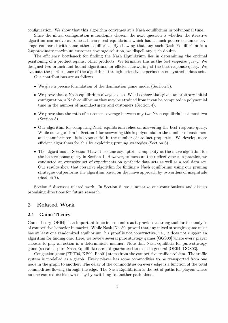
Definition 1 Let α = (p1, ..., pt) be a configuration. Let Wi(α) ⊆ C be the set of customers domi-nated by pi ∈ α. Then the effective dominating point of pi is a point e(pi, α) = (e[1], e[2], . . . , e[d])such that e[k] := mincj∈Wi(α) cj [k], 1 ≤ k ≤ d.

11

p

X

Y

O

) , ( a p e 2 c

1 c

Figure 2: Example for effective dominating point

In Figure 2, we show an example of an effective dominating point, e(p, α) for the point p.From the figure, we can see that the effective dominating point is actually the top-most right-mostposition in the multidimensional space which can dominate exactly same set of customers as thegiven point p.

Definition 2 Let e = (e[1], ..., e[d]) be an effective domination point. Then the domination re-gion of e is the subset of the d-dimensional product attribute space, such that every point in it isdominated by e.

In Figure 2, the domination region of e(p, α) is right top part of the 2-dimensional space boundedby two lines from e(p, α). The following lemma shows an important property of effective dominatingpoint.

Lemma 5 Given a product pi and its effective dominating point e(pi, α), there is at least onecustomer point on each face of the region dominated by e(p, α).

Proof: If there is no point on a face of the dominating region on attribute dimension Ak,mincj∈Wi(α) cj [k] must be larger than e(pi, α)[k], which is contradictory to the definition of effectivedominating point. 2

In Figure 2, customer point c1 and c2 are the customer points on the two faces of dominationregion of e(p, α) respectively.

Let C ⊆ C denote a subset of customers in the game, and λ(C) be the most top right pointdominating all customers in C. We have:

Lemma 6 For any product point p located on the hyperplane hi, e(p, α) = λ(C) for some C ⊆ Csuch that |C| ≤ d.

Proof: Let Wi(α) be set of customers dominated by p. For each dimension Ak, we pick one ofthe customers from Wi(α), with the smallest value along the dimension and add the customer intoC. C thus contains at most d customers and λ(C) is definitely able to dominate all customers inWi(α), making it equal to e(p, α). 2

When a customer has the smallest values on several different dimensions, the size of set C willbe smaller than d. We note that given any customer subset C of size no larger than d, it is notnecessary to have a plausible product point p on the hyperplane hi to satisfy e(p, α) = λ(C). For

12

1 c 2 c 3 c

, 2 1 c c , 3 1 c c , 3 2 c c

Figure 3: Example for customer search tree

a hyperplane Σdk=1bikpi[k] = xi, we say a point q is above hi if Σd

k=1bikq[k] > xi. Otherwise, it isbelow hi. We can show:

Lemma 7 If p∗i is the best response for mi on a configuration α, any product positioning pi abovehi and dominating e(p∗i , α) can achieve the same expected market share as p∗i . 2

The proof of the lemma is straightforward. In Figure 2, for example, any product dominatinge(p, α) dominates at least the five customers dominated by e(p, α).

Lemma 7 shows that given the effective dominating point of an optimal response pi, it is trivialto find a product achieving the same expected market share on the hyperplane hi. This implies anew best response searching method. We can try all combinations of customers with size no largerthan d, find the combination C ′ which give the highest expected market share based on λ(C ′), andsimply use the projection of λ(C ′) on hi as the final optimal result.

6.1.2 Customer Search Tree

Based on the analysis earlier, we propose a new concept, called Customer Search Tree, for findinga customer combination that gives the maximum expected market share.

Assuming an arbitrary global order on the customers, C = c1, c2, . . . , cn, subsets of C can berepresented as strings in the obvious way. We assume this below. Given two customer subsets Cq

and Cr, Cr is the extension of Cq if Cr = Cq · c for some customer c 6∈ Cq.A search tree structure, L(C), is constructed based on the above definitions. Every node in the

search tree represents a customer set Cq ⊆ C of size no larger than d. Without ambiguity, we useCq to denote both a customer set and the node in the search tree that represents it. There is adirected edge from Cq to Cr, iff Cr is an extension of Cq. The nodes and edges form a tree withroot at the empty node. We say a node Cr is the descendant of Cq if there exists a directed pathfrom Cq to Cr in the search tree.

Thus, the searching process over all the combinations of customers can be accomplished bymoving through the search tree nodes along the edges.

In Figure 3, we present an example of the customer search tree, on a data set with 3 customersin 2 dimensional space. c1, c2 and c1, c3 are extensions of c1 by definition.

Lemma 8 If Cr is a descendant of Cq in L(C), the domination region of λ(Cr) must cover thedomination region of λ(Cq).

Proof: If e1 = λ(Cr) and e2 = λ(Cq), e1[k] = mincj∈Cr cj [k] and e2[k] = mincj∈Cq cj [k]. SinceCq ⊂ Cr, e1[k] ≤ e2[k]. So, the domination region of λ(Cr) must cover that of λ(Cq). 2

Given a node Cq and one of its descendants Cr, we say Cr extends Cq on dimension Ak, ife1[k] < e2[k] where e1 = λ(Cr) and e2 = λ(Cq).

13

Algorithm 2 Breadth/Depth First Search (Customer Search Tree L, Hyperplane hi)1: while there is at least one node in L not pruned or not visited do2: Find the next search tree node N in breadth/depth first order3: Construct effective dominating point e = λ(N)4: if e is above hi using Property 2 of profit constraint hyperplane then5: Compute the expected market share of e (section 6.2)6: Update the best response if e is better than current solution7: Prune the children of N (section 6.3)8: Project the best e onto hi and return the result

6.1.3 Searching on Customer Search Tree

To find the customer combination C ′ such that λ(C ′) can achieve optimal expected marketshare, we employ two different searching strategies over the search tree L(C), namely breadth firstsearch and depth first search 2. Starting at the root of L(C), the algorithms iterate through thenodes in the search tree in different order, but have the same operations at any single node C ′.They compute e = λ(C ′) and calculate the expected market share at e based on the configuration ofother manufacturers. If e is better than the current best response, e will become the best response.Some pruning are conducted to reduce the number of nodes that must be visited. After all thenodes that are reachable from the root has been visited, the algorithm projects the optimal positione onto hi to obtain the final result as the best response.

In the rest of the section, we will discuss the detail on how the expected market share at λ(C ′)can be efficiently computed (section 6.2), as well as how we can prune children node which aredefinitely unable to give better result (section 6.3).

6.2 Computing Expected Market Share Based on R-Tree

Given a node C ′ in the search tree node with k customers, e = λ(C ′) is computed by retrieving thesmallest value of the k customers on every dimension. If e is below the profit constraint hyperplaneof the manufacturer, then e is not a valid position since it violates the constraint. If e is above thehyperplane, we need to efficiently determine the expected market share that e will bring.

To efficiently support such an operation, we use a modification of the R-Tree index [Gut84],called aggregation R-tree [JL98, LM01, PKZT01]. Every point in the R-Tree is a customer pointin the data set. A weight is assigned to every point in the R-Tree representing the expectedmarket share it can provide if a product dominates it. If there are already s products dominating acustomer cj , the weight of cj is 1/(s + 1). Thus, the expected market share λ(C) can be computedby summing up the weight of all the customers that it can dominate. Since the details of suchoperations are well studied in [JL98, LM01, PKZT01], we suppress further details here. By someanalysis of the studies on such indexing structure, the complexity of the computation is aboutO(log n), where n is the number of customers indexed. To update the weights of the nodes becauseof the changing number of dominators, the algorithm needs to iterate and update every node in theindexing tree, after every iteration. The cost of such update is affordable, since the update timedepends on the number of nodes in the indexing tree, usually O(n log n), which is much cheaperthan the time spent on iterations over the customer search tree.

6.3 Pruning Strategies

In order to reduce the number of nodes being visited in the search tree, we propose two pruningconditions which will be applied in Line 7 of Algorithm 2.

14

X

Y

O

e

' e

Figure 4: Example of Upper Bound

6.3.1 Boundary Condition

Given an effective dominating point e, Lemma 5 has already shown that there is at least one cus-tomer on every face of its domination region. Here, provide a boundary condition which constrainsthe nodes visited in the search tree.

We say a customer set C ⊆ C satisfies the boundary condition, if every customer c ∈ C is theunique point with the minimum value in some dimension. That is, there is at least one dimension,the boundary on which is only decided by this customer. We have the following lemma.

Lemma 9 Given a node C not satisfying the boundary condition, there must exist another nodeD ⊆ C satisfying boundary condition, and λ(D) = λ(C). For any descendant C ′ of C, there existsa descendant node D′ of D, such that λ(D′) = λ(C ′). 2

Proof: Assume C ′ has k different customer points c1, . . . , ck, and without generality ck is notthe only point on any domination face of λ(C ′). Then, by removing ck, we have a node D′ withk − 1 points, λ(D′) = λ(C ′) since the removal of ck can not increase the minimum value of D′ onany dimension. If C ′′ is a descendant of C ′ by combining C ′ with another customer subset F , thatis C ′′ = C ′ ∪ F , we can find the corresponding descendant D′′ of D′ by combining D′ and F . It iseasy to verify that λ(D′′) = λ(C ′′). 2

Suppose Algorithm 2 currently visits node C. By the above lemma, any child (and hencedescendants) of C not satisfying the boundary condition can be pruned from further considerations.

6.3.2 Upper Bound Pruning

By extending from a customer set C to any of its descendant C ′, the expected market share willdefinitely be non-decreasing since the domination region of λ(C) will grow by Lemma 8. However,we will show that it is possible to derive an upper bound on the expected market share of λ(C ′)based on the current information in C.

Lemma 10 In computing the best response for manufacturer mi with profit constraint hyperplanehi given by

∑dk=1 bikpi[k] = xi, let e = λ(C) = (e[1], e[2], . . . , e[d]) for a node C. Let C ′ be any

descendant of C in the customer search tree and let e′ = λ(C ′) = (e′[1], . . . , e′[d]). Then for anydimension k, e′[k] ≥ e[k]− (

∑e[k]bik − xi)/bik.

15

Algorithm 3 ExtensibleUpperBoundTest (customer subset C ′, profit constraint hyperplanehi, R-Tree root r, threshold θ)1: e = λ(C ′)2: for every dimension combination set ω do3: if ω is extensible by Definition 11 then4: Construct the upper bound point p′ = X(e, ω)5: if DomCount(p′, r) > θ then6: Return without pruning7: Prune all the children of C ′

Proof: Since any descendant node C ′ must contain more customers than C, the boundary of λ(C ′)on any dimension cannot be larger than that of λ(C), i.e. e′[k] ≤ e[k]. If e′[k] < e[k]− (

∑j e[j]bij−

xi)/bik for some k, we have∑

j e′[j]bij < e[k]bik − (∑

j e[j]bij − xi) +∑

j 6=k e[j]bij = xi, making thepoint λ(C ′) below the hyperplane. 2

Thus, for a point e = λ(C) above hi, we define the upper bound point U(e) = (eu[1], . . . , eu[d])with eu[k] = e[k] − (

∑e[k]bik − xi)/bik. It is obvious that U(e) dominates λ(C ′) where C ′ is any

descendant of C. Thus, the expected market share of U(e) is an upper bound on the expectedmarket share achievable on the descendants of C.

Note that Lemma 10 works only when the hyperplane follows the constraint∑d

k=1 bikpi[k] = xi.It is not hard to extend it to any hyperplane satisfying Property 2 in Section 3, by which theminimum possible value on each dimension can be calculated in constant time.

In Figure 4, we show an example of the upper bound computation in 2-dimensional space. Thepoint e′ is U(e) for the point e above the hyperplane.

From the figure, we can see that the upper bound on the market share by directly expandingalong all dimensions can be very loose. Fortunately, we can tighten the bound by combining Lemma9 with the boundary condition since extension on all dimensions can violate the boundary conditionin Lemma 9.

Assume C = c1, c2, . . . , ck is the node being visited in the search tree. Let DS(ci, C) =Ao1 , Ao2 , . . . 1 ≤ ok ≤ d, denoting the set of dimensions such that ci is on the face of dominationregion for λ(C) along these dimensions. In Figure 5, for example, there are three dimensionsx, y, z. If C = c1, c2, where c1 = (1, 1, 2), c2 = (2, 2, 1) and λ(C) = e = (1, 1, 1), thenDS(c1, C) = x, y and DS(c2, C) = z because c1 has minimum values on dimension x and ywhile c2 has minimum value on dimension z.

Definition 3 A set of dimensions ω is an extensible dimension set for a customer subset C if|DS(cj , C)− ω| > 0 for every cj ∈ C.

In the definition above, DS(cj , C) − ω is the set of the dimensions in DS(cj , C) but not in ω.Recall the example in Figure 5. x is an extensible dimension set, since DS(c1, C) − x = yand DS(c2, C) − x = z. However, x, z is not, since DS(c2, C) − x, z = ∅. The extensibledimension set has the property shown in the next lemma.

Lemma 11 If a descendant C ′ of C extends along some dimensions which is not in the extensibledimension set ω, C ′ must violate the boundary condition. 2

Proof: If a dimension set ω is not an extensible dimension set, there is at least one point cj ∈ C ′

that |DS(cj , C′)− ω| = 0. Then, cj can not be on any face of the domination region of C ′′, which

contradicts boundary condition. 2

16

) 1 , 1 , 1 ( e

y

x

z

) 2 , 1 , 1 ( 1 c

) 1 , 2 , 2 ( 2 c

Figure 5: Example of extensible dimension set

By the last lemma, the descendants of C can only extend the dominating region of λ(C) onthose extensible dimension sets. Given an extensible dimension set ω and e = λ(C), we proposethe extensible upper bound point X(e, ω) = (eω[1], eω[2], . . . , eω[d]), s.t. eω[k] = e[k] if k 6∈ ω andeω[k] = eu[k] otherwise. It is clear that the expected market share of X(e, ω) must be the upperbound of the descendants of C by extending on ω.

Thus we propose the extensible upper bound computation algorithm in Algo 3. In this algo-rithm, we iterate through all the possible 2d−1 dimension combinations, and test the upper boundonly when the dimension combination is extensible. For example, in Figure 5, there are only twoextensible dimension sets, x and y, for C ′ = c1, c2. For all extensible dimension sets, if theexpected market share of the corresponding extensible upper bound point cannot be larger thanthreshold θ (the expected market share of the current best solution), the algorithm will prune allthe children of C ′. Since d is usually much smaller than n, the cost of iterating all dimension setsis typically small.

6.4 Discussion on Discretization

Another possible optimization for best-response query is the discretization over the dimensionswith continuous values. Given a d-dimensional unit space [0, 1]d, a customer cj is represented bya vector (cj [1], cj [2], . . . , cj [d]) in the original space. Given the specified discretization parameter∆, the original vector can be transformed to a new vector (bcj [1]/∆c∆, . . . , bcj [d]/∆c∆). By suchtransformation, the number of possible values on any dimensions is no more than d1/∆e, which canbe regarded as a constant number. Best response query can thus be answered by employing someexisting indexing technique, such as DADA-tree [LOTW06]. Although beyond the scope of thispaper, note that the efficiency of best response query can be dramatically improved, as is shown in[Li].

However, the customer data set has some loss on the detailed information of the customers,which may lead to some sub-optimal result of the best response query. While the convergenceresult of the domination game depends on the exact solution of best response query, the game maynot converge if any approximate best response is applied. Based on this observation, we only focus

17

on testing the algorithms outputting exact best response in the following experimental section.

7 Experiments

We carried out an experimental study to verify the properties and test the performances of thealgorithms proposed in this paper. The programs are compiled by gcc 3.4.3 and run on IBM x255server with four Intel Xeon MP 3.0 GHz CPU, 18G DDR memory and six 73.4GB Ultra320 SCSIhard disks.

In the experiments, we generate different types of synthetic data sets. All of the points inthe data sets are in [0, 1]d, where d is the dimensionality. The values on every dimension are allfloat numbers. The size of the customer set ranges from 1000 to 10000. The dimensionality of themarket varies from 2 to 4, while there are at least 2 and at most 9 corporations in the market.The default setting of the parameters above is 1000 customers, 3 dimensions and 2 corporations.There are four optional distributions of customer set, including Anti-Correlated (A), Correlated (C),Independent (I) and Clustered (L). In anti-correlated customer set, the increase of the requirementon one dimension will lead to some decrease on the others. In correlated customer set, a customerhaving high requirement on one dimension is likely to have similar high standards on the others.In independent customer set, all dimension are independent and obeys uniform distribution on therange. In clustered data set, the points are generated from 5 different Gaussian distributions in thespace.

We also employ a real data based on the review comments collected from a hotel review web siteTripAdvisor 8. The users of the web site are supposed to rate the hotels on 7 different attributes,as well as an overall score. All of the ratings are integers between 1 and 5. However, only fourattributes, including cleanliness, value, service and rooms, are used in our data since most of usersrate on all of them. Based on the assumption that a good overall score is given only when the hotelsatisfies all requirements of the user, we transform the review data set to requirement data set byusing the review tuples with overall scores no smaller than 4. After crawling 50 hotels in Sydney,we retrieve 997 valid tuples, each attribute of which is normalized to some real number between 0and 1. These tuples are regarded as customers in our experiments.

The profit constraint hyperplanes for the manufacturers are generated by uniformly choosingthe parameters bij and xi in the range of [0.8, 1.2], on synthetic data sets as well as on real dataset.

In our experiments, we focus on the efficiency of the algorithms proposed in this paper. In therest of the section, we use NAIVE, DFS and BFS to denote the iterative best response algorithmwith naive, depth first search and breadth first search as the underlying best response computationrespectively. In Table 2, we first compare the speed of NAIVE, DFS and BFS on 3 dimensionalspace with 1000 customers and 3 manufacturers. NAIVE is much slower than DFS and BFS onanti-correlated, correlated and independent data sets. This result indicates that lattice search is agreat improvement on the naive search scheme for best response query. Since NAIVE is not scalableto any larger or higher dimensional data sets, we only compare our DFS and BFS algorithm in therest of the experiments. On clustered data set, however, naive algorithm is not so bad because thesearching space is not large, which constrains the pruning ability of DFS and BFS.

In Figure 6, we show the computation cost of DFS and BFS on varying data size from 1000to 10000. The time spent by the two algorithms both increases polynomially with the expansionof the data set. DFS algorithm is a little better than BFS in all types of data sets, especially onclustered data sets.

8www.tripadvisor.com

18

Data Type A C I LNAIVE 5326 472 2163 31DFS 130 27 69 23BFS 132 29 73 25

Table 2: Speed comparison of NAIVE, DFS and BFS in seconds

10

100

1000

10000

100000

1 2 3 4 5 6 7 8 9 10

Tim

e (S

econ

ds)

Data Size (1000)

DFSBFS

(a) Correlated

10

100

1000

10000

100000

1 2 3 4 5 6 7 8 9 10

Tim

e (S

econ

ds)

Data Size (1000)

DFSBFS

(b) Independent

100

1000

10000

100000

1e+06

1 2 3 4 5 6 7 8 9 10

Tim

e (S

econ

ds)

Data Size (1000)

DFSBFS

(c) Anti-Correlated

10

100

1000

10000

100000

1 2 3 4 5 6 7 8 9 10

Tim

e (S

econ

ds)

Data Size (1000)

DFSBFS

(d) Clustered

Figure 6: Tests on varying data size

0.1

1

10

100

1000

432

Tim

e (S

econ

ds)

Dimensionality

DFSBFS

(a) Correlated

0.1

1

10

100

1000

10000

100000

432

Tim

e (S

econ

ds)

Dimensionality

DFSBFS

(b) Independent

0.1

1

10

100

1000

10000

100000

432

Tim

e (S

econ

ds)

Dimensionality

DFSBFS

(c) Anti-Correlated

0.1

1

10

100

1000

10000

432

Tim

e (S

econ

ds)

Dimensionality

DFSBFS

(d) Clustered

Figure 7: Tests on varying dimensionality

19

50

100

150

200

250

2 3 4 5 6 7 8 9T

ime

(Sec

onds

)

Corporation Number

DFSBFS

(a) Correlated

100

150

200

250

300

350

400

450

500

550

2 3 4 5 6 7 8 9

Tim

e (S

econ

ds)

Corporation Number

DFSBFS

(b) Independent

200

300

400

500

600

700

800

2 3 4 5 6 7 8 9

Tim

e (S

econ

ds)

Corporation Number

DFSBFS

(c) Anti-Correlated

20

40

60

80

100

120

140

160

180

200

2 3 4 5 6 7 8 9

Tim

e (S

econ

ds)

Corporation Number

DFSBFS

(d) Clustered

Figure 8: Tests on varying manufacturer number

As is shown in Figure 7, the computation times of DFS and BFS are still exponential in thedimensionality d. However, by some simple linear regression on the curves, we can verify that theempirical time complexity of DFS and BFS on dimensionality d is proportional to 100d. Since thereare n = 1000 points in the data set, the lattice search algorithm on DFS and BFS still achieve someimprovement on NAIVE.

We also conduct some experiments on varying the number of manufacturers in the market. Theresult in Figure 8 shows that the linear increase of computation time implies that the iterationnumber of the process also increases linearly. When there are 9 manufacturers, the computationcost even decreases on independent and clustered data. This is because the data are so scatteredor grouped in these data sets that the manufacturers can easily target a small group of customersin the first iteration and find it hard to attract new customers with old customers kept. Thus, thestability of the market can be achieved easily even when there are more competitions in the samemarket.

Finally, the performance comparisons on the two algorithm over TripAdvisor data set is pre-sented in Figure 9. This group of test confirms the advantage of DFS over BFS on efficiency.DFS algorithm is almost two times faster than BFS algorithm when the number of manufacturersincreases from 2 to 6.

8 Conclusion and Future Work

In this paper, we proposed domination games for modelling competition among manufacturers ofa product for maximizing their expected market share. This work was motivated by the seminalwork of [KPR98b] motivating data mining from a microeconomic, utility oriented perspective.For domination games, we show that a Nash equilibrium always exists and showed that it canbe computed in polynomial time in the number of customers and products. The algorithm isexponential in the number of product properties. We developed speeding up strategies for answering

20

0

100

200

300

400

500

600

2 2.5 3 3.5 4 4.5 5 5.5 6

Tim

e (S

econ

ds)

Corporation Number

DFSBFS

Figure 9: Tests on varying manufacturer number with TripAdvisor data set

the best response query which forms the backbone of the algorithm for finding equilibria. Weshowed that in terms of customer coverage any Nash equilibrium is at most two times worse thanthe best one. Characterizing the complexity of the best response query in terms of dimensionality isopen. Extension of this framework where a customer may buy more than one model, or a productdominates a customer if it can satisfy the customer on k out of d dimensions, or there are multipleproduct types, or a customer buys a product with a probability determined by the proximity ofthe product to his preferences are all interesting directions for future work.

References

[BKS] S. Borzsonyi, D. Kossmann, and K. Stocker. The skyline operator. In ICDE’01.

[BSVW99] Tom Brijs, Gilbert Swinnen, Koen Vanhoof, and Geert Wets. Using association rulesfor product assortment decisions: A case study. In KDD, pages 254–260, 1999.

[CET05] Chee-Yong Chan, Pin-Kwang Eng, and Kian-Lee Tan. Stratified computation of sky-lines with partially-ordered domains. In SIGMOD, pages 203–214, 2005.

[CGGL03] Jan Chomicki, Parke Godfrey, Jarek Gryz, and Dongming Liang. Skyline with presort-ing. In ICDE, pages 717–816, 2003.

[CJT+06] C.-Y. Chan, H. V. Jagadish, K.-L. Tan, Anthony K. H. Tung, and Z. Zhang. Findingk-dominant skylines in high dimensional space. In SIGMOD, pages 503–514, 2006.

[DPS02] Xiaotie Deng, Christos H. Papadimitriou, and Shmuel Safra. On the complexity ofequilibria. In STOC, pages 67–71, 2002.

[DPSV02] Nikhil R. Devanur, Christos H. Papadimitriou, Amin Saberi, and Vijay V. Vazirani.Market equilibrium via a primal-dual-type algorithm. In FOCS, pages 389–395, 2002.

[DS07] Evangelos Dellis and Bernhard Seeger. Efficient computation of reverse skyline queries.In VLDB, pages 291–302, 2007.

[ea75] H. T. Kung et. al. On finding the maxima of a set of vectors. In JACM, 22(4), 1975.

[EGJH04] Martin Ester, Rong Ge, Wen Jin, and Zengjian Hu. A microeconomic data miningproblem: customer-oriented catalog segmentation. In KDD, pages 557–562, 2004.

[FPT04] Alex Fabrikant, Christos H. Papadimitriou, and Kunal Talwar. The complexity of purenash equilibria. In STOC, pages 604–612, 2004.

21

[GGS03] Georg Gottlob, Gianluigi Greco, and Francesco Scarcello. Pure nash equilibria: hardand easy games. In TARK ’03: Proceedings of the 9th conference on Theoretical aspectsof rationality and knowledge, pages 215–230, 2003.

[GSG05] Parke Godfrey, Ryan Shipley, and Jarek Gryz. Maximal vector computation in largedata sets. In VLDB, pages 229–240, 2005.

[Gut84] A. Guttman. R-trees: A dynamic inde structure for spatial searching. In SIGMOD’84,pages 47–57, 1984.

[HJLO06] Zhiyong Huang, Christian S. Jensen, Hua Lu, and Beng Chin Ooi. Skyline queriesagainst mobile lightweight devices in MANETs. In ICDE, page 66, 2006.

[JL98] Marcus Jurgens and Hans-Joachim Lenz. The ra*-tree: An improved r-tree with ma-terialized data for supporting range queries on olap-data. In DEXA Workshop, pages186–191, 1998.

[JTEH07] W. Jin, A.K.H. Tung, M. Ester, and J. Han. On efficient processing of subspace skylinequeries on high dimensional data. 2007.

[KP99] Elias Koutsoupias and Christos H. Papadimitriou. Worst-case equilibria. In STACS,pages 404–413, 1999.

[KPR98a] J. Kleinberg, C.H. Papadimitriou, and P. Raghavan. Segmentation problems. In STOC,1998.

[KPR98b] J. Kleinberg, C.H. Papadimitriou, and P. Raghavan. A microeconomic view of datamining. In Data Min. Knowl. Discov., 2(4): 311-322, 1998.

[KRR] D. Kossmann, F. Ramsak, and S. Rost. Shooting stars in the sky: an online algorithmfor skyline queries. In VLDB’02.

[Li] Xin Li. Honor year report: Rtree-based dada for dominant relationship queries anddomination game model. https://dl.comp.nus.edu.sg/dspace/handle/1900.100/2487.

[LM01] Iosif Lazaridis and Sharad Mehrotra. Progressive approximate aggregate queries witha multi-resolution tree structure. In SIGMOD Conference, pages 401–412, 2001.

[LOTW06] Cuiping Li, Beng Chi Ooi, Anthony K.H. Tung, and Shan Wang. Dada: a data cubefor dominant relationship analysis. In SIGMOD, 2006.

[LTJE07] Cuiping Li, Anthony K. H. Tung, Wen Jin, and Martin Ester. On dominating yourneighborhood profitably. In VLDB, pages 818–829, 2007.

[Nas50] J. F. Nash. Equilibrium points in n-person games. Proc. of National Academy ofSciences, 36:48–49, 1950.

[OR94] M. J. Osborne and A. Rubinstein. A Course in Game Theory. The MIT Press, 1994.

[Pap01] Christos H. Papadimitriou. Algorithms, games, and the internet. In STOC, pages749–753, 2001.

[PKZT01] Dimitris Papadias, Panos Kalnis, Jun Zhang, and Yufei Tao. Efficient olap operationsin spatial data warehouses. In SSTD, pages 443–459, 2001.

22

[PTFS03] D. Papadias, Y. Tao, G. Fu, and B. Seeger. An optimal and progressive algorithm forskyline queries. In SIGMOD, 2003.

[SS06] Mehdi Sharifzadeh and Cyrus Shahabi. The spatial skyline queries. In VLDB, pages751–762, 2006.

[Ste86] R. Steuer. Multiple Criteria Optimization. Wiley, New York, 1986.

[TEO01] K. L. Tan, P. K. Eng, and B. C. Ooi. Efficient progressive skyline computation. InVLDB, 2001.

[TXP07] Yufei Tao, Xiaokui Xiao, and Jian Pei. Efficient skyline and top-k retrieval in subspaces.IEEE Trans. Knowl. Data Eng., 19(8):1072–1088, 2007.

[Vet02] Adrian Vetta. Nash equilibria in competitive societies, with applications to facilitylocation, traffic routing and auctions. In FOCS, pages 416–428, 2002.

[WFW03] Raymond Chi-Wing Wong, Ada Wai-Chee Fu, and Ke Wang. Mpis: Maximal-profititem selection with cross-selling considerations. In ICDM, pages 371–378, 2003.

[WOTX07] Shiyuan Wang, Beng Chin Ooi, Anthony K. H. Tung, and Lizhen Xu. Efficient skylinequery processing on peer-to-peer networks. In ICDE, pages 1126–1135, 2007.

[WTB04] J. X. Zheng W.-T. Balke, U. Guntzer. Efficient distributed skylining for web informa-tion systems. In EBDT, 2004.

[WZF+06] Ping Wu, Caijie Zhang, Ying Feng, Ben Y. Zhao, Divyakant Agrawal, and Amr ElAbbadi. Parallelizing skyline queries for scalable distribution. In EDBT, pages 112–130, 2006.

[WZH02] Ke Wang, Senqiang Zhou, and Jiawei Han. Profit mining: From patterns to actions.In EDBT, pages 70–87, 2002.

[XZ06] Tian Xia and Donghui Zhang. Refreshing the sky: the compressed skycube with effi-cient support for frequent updates. In SIGMOD, pages 491–502, 2006.

[Yao03] J. T. Yao. Sensitivity analysis for data mining. In Proceedings of The 22nd InternationalConference of NAFIPS (the North American Fuzzy Information Processing Society),pages 272–277, 2003.

[YLL+05] Yidong Yuan, Xuemin Lin, Qing Liu, Wei Wang, Jeffrey Xu Yu, and Qing Zhang.Efficient computation of the skyline cube. In VLDB, pages 241–252, 2005.

23