On environmental contours for marine and coastal design.

Emma Rossa, Ole Christian Astrupb, Elzbieta Bitner-Gregersenb, Nigel Bunnc, Graham Feldd,Ben Gouldbyc, Arne Husebye, Ye Liuc, David Randella, Erik Vanemb, Philip Jonathanf,g,∗

aShell Global Solutions B.V., 1031 HW Amsterdam, The Netherlands.bDNV-GL, 1363 Hovik, Norway.

cHR Wallingford, Wallingford OX10 8BA, United Kingdom.dShell UK Ltd., Aberdeen AB12 3FY, United Kingdom.

eDepartment of Mathematics, University of Oslo, 0316 Oslo, Norway.fShell Research Ltd., London SE1 7NA, United Kingdom.

gDepartment of Mathematics and Statistics, Lancaster University, Lancaster LA1 4YW, United Kingdom.

Abstract

Environmental contours are used in structural reliability analysis of marine and coastal structuresas an approximate means to locate the boundary of the distribution of environmental variables, andhence sets of environmental conditions giving rise to extreme structural loads and responses. Outlineguidance concerning the application of environmental contour methods is given in recent designguidelines from many organisations. However there is lack of clarity concerning the differencesbetween approaches to environmental contour estimation reported in the literature, and regardingthe relationship between the environmental contour, corresponding to some return period, and theextreme structural response for the same period. Hence there is uncertainty about precisely whenenvironmental contours should be used, and how they should be used well. This article seeks toprovide some assistance in understanding the fundamental issues regarding environmental contoursand their use in structural reliability analysis. Approaches to estimating the joint distributionof environmental variables, and to estimating environmental contours based on that distribution,are described. Simple software for estimation of the joint distribution, and hence environmentalcontours, is illustrated (and is freely available from the authors). Extra assumptions required torelate the characteristics of environmental contour to structural failure are outlined. Alternativeresponse-based methods not requiring environmental contours are summarised. The results of aninformal survey of the metocean user community regarding environmental contours are presented.Finally, recommendations about when and how environmental contour methods should be used aremade.

Keywords: extreme, structural reliability, return value, environmental contour, structuralresponse, joint probability, IFORM.

∗Corresponding author. Email: philip.jonathan@shell.com

Preprint submitted to Ocean Engineering December 17, 2018

1. Introduction

1.1. Metocean design

Currently, numerous approaches for establishing design criteria for metocean loads and responsesof marine structures and coastal facilities are used by different practitioners. Some of these areincluded in marine industry standards and guidelines; others are internal standards of different or-ganisations active in ocean engineering. Rigorous comparison of some approaches has been reportedin the literature, but there is still uncertainty in the user community regarding the relative meritsof different approaches. Within the marine industry, estimation of a joint metocean description hasbeen considered for more than thirty years. It was shown that typically, environmental forces onmarine structures may be reduced by 5% to 40% by accounting for the lack of complete dependencebetween metocean variables (wind, wave, current, etc.) traditionally used in design (e.g. E&P Fo-rum 1985, Feld et al. 2018). Development of reliability methods (e.g. Madsen et al. 1986) andtheir implementation by some parts of the industry in the 1980s brought joint probabilities intofocus: they are required for a consistent treatment of the loading in Level III reliability analysisand for assessment of the relative importance of various metocean variables during extreme loadand response conditions, fatigue damage and at failure.

Until the middle of the 1990s, very few metocean data sets of sufficient quality were available,limiting development of joint probability models: this has changed during the last twenty years.Comprehensive hindcast data are now available for locations world-wide, including simultaneousvalues for wind, waves, current, sea water level, ice and snow of sufficient quality and duration.Today joint probabilities are referenced in industry standards and guidelines (e.g. IACS 2001,DNVGL-RP-C205 2017, NORSOK N-003 2017, ISO19901-1 2015). They are required for applica-tion of the Formal Safety Assessment (FSA) methodology in rule development, providing risk basedgoal-oriented regulations that are well balanced with respect to acceptable risk levels and economicconsiderations, as recommended in IMO (2001).

Different standards describing the application of joint probability methods exist. ISO19901-1 (2015), DNVGL-RP-C205 (2017) and NORSOK N-003 (2017) suggest that joint probabilitymethods should be applied if reliable simultaneous data exist. NORSOK N-003 (2017) furtherrecommends that the duration of a data should be sufficiently long to capture the probability ofoccurrence for all combinations of importance regarding predictions of metocean actions and actioneffects. Further, in a case of wind, wave and current it recommends that at least three yearsof simultaneous data is required to characterise the lack of complete dependence between thesevariables reliably in design.

Given that it is possible to establish a model for the “short-term” distribution of response givensea state parameters (for example, for a three hour sea state), NORSOK N-003 (2017) states thatthe designer has essentially three different risk-based approaches to estimating the “long-term”distribution of response (corresponding to hundreds or thousands of years): a) the so-called “allshort-term conditions” (or “all sea state”) approach, b) the “storm event“ approach, and c) theenvironmental contour method, an approximate method using only short-term analysis.

There are two distinct joint probability approaches in widespread use in coastal engineering prac-tice in the UK (e.g. DEFRA / Environment Agency 2005). These are (a) a simplified method thatinvolves the use of joint probability contours (JPC) and (b) a risk-based statistical method. Bothapproaches are implemented within the widely-used JOIN-SEA software system (HR Wallingford1998; Hawkes et al. 2002).

2

1.2. Environmental contours

The environmental contour defines a set of extreme sea state conditions, and can be used toapproximate extreme values of long-term structural response extremes by considering only a fewshort-term metocean conditions. Environmental contours are appealing since they can be speci-fied for a given metocean environment independently of any structure; they are also linked to awell-established approach to structural design, familiar to practitioners. To establish them, jointprobabilities of metocean parameters, historically in the metocean community in the form of ta-bles, are needed. The idea behind the method is to define contours in the metocean space (forexample, HS , TP ) along which extreme responses with given return period should lay. It is a sim-plified and approximate method compared with full long-term response analysis but requires lesscomputational effort.

All environmental contour methods have a common goal of summarising the tail of the jointdistribution of environmental variables, with a view to learning about the distribution of extremestructural response within a prescribed return period. This is achieved by identifying combinationsof environmental variables (sometimes referred to as governing conditions) responsible for extremestructural response. Structural responses for combinations of environmental conditions lying on thecontour can be used to estimate the extreme response due to a sea state with the same return periodas the contour. Importantly, only combinations of metocean parameters lying on the contour needbe considered. With additional a priori knowledge of the response, it is possible to limit the intervalof the contour over which to evaluate structural response, substantially reducing the computationaleffort for calculating extreme response. An underlying assumption is that the extreme N -yearresponse is governed by sea state conditions on the N -year environmental contour.

Contours estimated using different methods will be different in general, since each method makesdifferent assumptions in characterising the environment, or seeks to summarise the environment ina different way. Hence, the choice of environmental contour method will influence the estimationof the distribution of extreme response.

Nevertheless, the environmental contour approach may be useful for early phase concept eval-uation. For example, as stated by NORSOK N-003 (2017), if the application under considerationis of a very non-linear nature, an extensive model test program may be necessary to model theshort-term variability for all important metocean conditions; the environmental contour approachcan help identify those conditions.

Some approaches to estimation of environmental contours (for example IFORM, Wintersteinet al. 1993) make additional explicit assumptions regarding the nature of structural failure surfacesexpressed in terms of (potentially transformed) environmental variables. When these assumptionsare valid, statements regarding the relative magnitude of the exceedance probability of the N -yearenvironmental contour and the N -year structural failure probability can be made more reasonably.However it is not always clear that the additional assumptions are satisfied for a given application.

The environmental contour procedure as given by NORSOK N-003 (2017) can be summarised as:(a) Establish environmental contours of the metocean characteristics (e.g. HS , TP ) correspondingto some annual non-exceedance probability 1 − 1/T (for a T -year return period); (b) Identify theworst metocean condition along the contour for the response under consideration; (c) For this seastate, determine the distribution function for the appropriate three-hour (or possible one-hour)extreme value for the response under consideration; and (d) Estimate the value of the response(corresponding to the same annual non-exceedance probability 1 − 1/T ) using the quantile ofthe distribution of response (from (c)) with non-exceedance probability α. A value α = 0.9 is

3

recommended for ULS (the ultimate limit state), and α = 0.95 for ALS (the accidental limit state).The standard provides some guidance as to the adequacy of the approach in terms of the widthof the distribution of response in (c). Although this standard discusses the environmental contourmethod for sea states of length three hours, the procedure can be applied to sea states of anyappropriate length (for example, 30 minutes); we use three-hour sea states here for consistency andease of explanation.

DNVGL-RP-C205 (2017) recommends two environmental contour approaches: IFORM (Win-terstein et al. 1993, procedure similar to NORSOK N-003 (2017) above), and a constant probabilitydensity approach (Haver 1987). The procedure for the latter can be summarised as: (a) Estimatea joint environmental model of sea state variables of interest; (b) Estimate the extreme value forthe governing variable for the prescribed return period, and associated values for other variables(for example, 100-year HS and conditional median TP ); and (c) Develop a contour line from thejoint model or scatter diagram as the contour of constant probability density going through theparameter combination mentioned above.

Using the environmental contour, an estimate of the extreme response is obtained by searchingalong the contour for the condition giving maximum characteristic extreme response. The contourmethod is affected by uncertainties related to metocean data and adopted joint models and has itsown limitations which are pointed out by DNVGL-RP-C205 (2017) and NORSOK N-003 (2017).It will tend to underestimate extreme response levels because it neglects short term variability ofresponse between different realisations of sea states. Both standards recommend approaches basedon Winterstein and Engebretsen (1998) to account for this, including (a) increasing the returnperiod corresponding to the contour, and hence inflating the environmental contours; (b) replacingthe stochastic response by a fixed fractile level higher than the median value; or (c) applyingmultipliers of the median extreme response estimates, to introduce more conservatism.

In the coastal engineering community, contours of joint exceedance probability of environmentalvariables are estimated using the JPC method (a) to find design events that form the boundaryconditions for numerical and physical models for the purposes of structural design; and (b) toestimate return values of overtopping and overflow rates corresponding to some return period foruse in flood mapping and risk analysis (CIRIA 1996, 2007). A series of combinations of values ofenvironmental variables from the contour are tested in order to find the worst case value of theresponse. This worst case value is then assumed to have the same return period as the returnperiod associated with the environmental contour. Since again, without further assumptions, thereis no link between environmental contour and structural response, there are obvious short-comingsto this approach, which are well recognised (e.g. Gouldby et al. 2017).

The performance of different environmental contour methods has been investigated in severalstudies, including work by some of the current authors (including Jonathan et al. 2014a; Vanem andBitner-Gregersen 2015; Gouldby et al. 2017; Vanem 2017). After consideration of the fundamentalmathematical differences between different contour methods, it is unreasonable in general to expectto find any consistent trends in comparisons of contour methods across different applications. Thecharacteristics of different environmental contour methods must be assessed on an application-by-application basis. There are a number of more fundamental reviews of environmental contourmethods, including excellent recent work by Haselsteiner et al. (2017).

1.3. End-user survey

As part of the ECSADES research project (see Section 7), a survey was conducted on end-userpractice in the use of environmental contours. The survey, receiving 19 respondents from industry

4

and academia, consisted of questions aimed at establishing the following: (a) Frequency of use ofenvironmental contours in structural reliability and design; (b) Variety in methods used to definethe contour and popular sources of guidance and literature; (c) Variety in application of contours(how is information from the contour used); and (d) Perceived advantages and disadvantages ofusing environmental contours.

Further details of the survey can be found in Appendix A.1. Two key insights resulted fromthe survey. Firstly, though respondents cited varying frequency of application of contours, theydid appear to agree on contours forming an integral part of reliability assessment and design.Respondents cited contours as an “industry-accepted approach to approximating N -year responsesquickly” (when compared to long-term time-domain methods), especially when there is little or noknowledge about the structure being designed - the same environmental contour potentially beingapplicable to a range of responses. Secondly, respondents cited that there is no single standardapproach to defining the contour nor to applying it in the estimation of responses. Seven key sourcesof guidelines were cited, part of a collection of over fifty relevant papers collected by the authorsof this paper. Further, respondents expressed concern over a lack of understanding of the meaningof the contours and the risks associated with naive application of statistical methods leading tophysically unreasonable contours. The level of interest in application offshore is greater in Norwaythan other locations, although coastal practitioners use contours widely.

These insights highlight the need for clarity both on the modelling choices available when definingcontours, and on the applicability of contours given the information available for a given structureand environment. We have attempted to address the majority of comments emerging from thesurvey in this paper

1.4. Objective and outline

The objective of this article is to (a) Overview the statistical ideas underpinning environmentalcontour methods, (b) Highlight fundamental differences between methods, (c) Explain the linkbetween environmental contour and structural failure probability claimed by some approaches, (d)Provide simple software to allow a metocean practitioner to estimate a sensible model for generalsettings (based on extreme value analysis of a historical sample from the environment), and (e)Provide basic guidance regarding when and how environmental contour methods should be usedsensibly.

The layout of the article is as follows. Section 2 discusses fundamental issues regarding the mean-ing and definition of return value in a multivariate setting, and lack of invariance of a probabilitydensity function under transformation of variables. It also discusses the procedure typically usedto estimate the distribution of so-called “long-term” statistics (such as the N -year maximum re-sponse) from “short-term” statistics (such as the distribution of maximum response in a three-hoursea state). Section 3 provides a description of different families of models for the joint distribu-tion of environmental variables. Section 4 outlines the different kinds of environmental contoursdiscussed in the literature. It also outlines a rationale to relate the characteristics of an environ-mental contour with a structural failure surface for some response, and describes an approach tomodify environmental contours to account for the short-term variability of maximum response in athree-hour sea state. Section 5 provides a discussion of case studies used to illustrate the competingcharacteristics of different environmental contour methods, and the challenges of linking contourwith response. Section 6 provides discussion, and a concluding protocol to aid the practitioner indeciding when and how to apply environmental contour approaches reasonably.

5

2. Return values, transformation of variables and long-term statistics

In this section, we start by considering the definition of a univariate return value, and considerthe issues in extending this concept to the multivariate case. We illustrate the sensitivity of theprobability density function for the joint distribution of environmental variables to transformationof variables. We also describe how the characteristics of a response for a sea state (“short-term”)can be used to estimate its characteristics over an extended period of time (“long-term”).

2.1. Univariate return values

Estimation of extremes for a single variable X is relatively straightforward and has been studiedextensively (e.g. Coles 2001). Given a representative set of independent observations of X spanningmany years, extreme value analysis can be used to estimate the distribution FMX,1

of the annualmaximum MX,1. This in turn can be used to estimate the T -year return value xT by solving theequation

Pr(MX,1 > xT ) = 1− FMX,1(xT ) = 1/T . (1)

The T -year return value xT for a single variable is therefore well-defined in terms of the tail of thecumulative distribution function FMX,1

of the annual maximum MX,1 of X.

2.2. Multivariate return values

Unfortunately, the joint return value for two or more variables (X,Y ) cannot be uniquely defined(e.g. Serinaldi 2015). For example, in the case of two variables (X,Y ), we could define the returnvalue (xT , yT ) in terms of the joint distribution FMX,1,MY,1

of the annual maxima MX,1,MY,1 using

Pr(MX,1 > xT ,MY,1 > yT ) = 1− FMX,1,MY,1(xT , yT ) = 1/T . (2)

However, it is immediately apparent that there is no unique solution to this equation; given anypair (xT , yT ) which satisfies the equation, we can increase xT slightly, and reduce yT such that theequation is still satisfied. That is, there is a continuum of solutions to the equation, which we canwrite as the set {xT (θ), yT (θ)} indexed by parameter θ ∈ C. As we vary θ, the pair (xT (θ), yT (θ))maps out a contour (corresponding to {xT (θ), yT (θ)}) of constant exceedance probability 1/T in(x, y)-space. We note for clarity, that a contour refers to a closed curve in some space ((x, y)-spacehere), on which the value of some function is constant.

We can rewrite the last equation as

Pr(MX,1 > xT ,MY,1 > yT ) = Pr(MY,1 > yT |MX,1 > xT ) Pr(MX,1 > xT ) = 1/T ,

motivating a definition of return value for the pair in terms of a marginal return value of MX,1

and a conditional return value of MY,1 given MX,1. Two boundary cases exist: (a) when MX,1

and MY,1 are perfectly correlated, points (xT , yT ) on the solution contour would satisfy Pr(MX,1 >xT ) = 1/T since Pr(MY,1 > yT |MX,1 > xT ) = 1 in this case, and (b) when MX,1 and MY,1 areindependent, solutions (xT , yT ) would satisfy Pr(MY,1 > yT ) Pr(MX,1 > xT ) = 1/T since nowPr(MY,1 > yT |MX,1 > xT ) = Pr(MY,1 > yT ). In general, the extent of dependence between pairMX,1 and MY,1 will be somewhere between perfect dependence (a) or independence (b).

To illustrate the importance of dependence in practice, we could for example choose to usethe 100-year maximum wave height, wind speed and current speed to estimate the environmental

6

loading with a return period of 100 years. If winds, waves and currents are perfectly correlated, theprobability of this combination of variables occurring would be 10−2 per annum as required. But ifthe variables were independent, the probability of this combination of variables occurring would be10−6 per annum, considerably less than 10−2. Some design codes and guidelines suggest taking the100-year return period of one (dominant) variable together with the values of associated variablescorresponding to shorter return periods to accommodate dependence between variables (e.g. Feldet al. 2018). The DNV recommended practice for on-bottom stability of pipelines suggests thecombination of the 100-year return condition for waves combined with the 10-year return conditionfor current or vice-versa, when detailed information about the joint probability of waves and currentis not available.

In summary: the concept of return value is not uniquely defined for more than one variable.In order to specify design values for more than one variable rationally, we need to understandand exploit the joint distribution of the variables. This leads naturally to consideration of jointprobabilities, of environmental contours, and of structure variables (such as structural responseto environmental loading) which capture the important joint characteristics of (a multivariate)environment in terms of a single “structure” or response variable (see Section 4).

2.2.1. Transformation of variables

Suppose we describe the environment in terms of variables (X,Y ) and a distribution with jointdensity fX,Y (x, y). Suppose further we choose also to describe the environment in terms of trans-formed variables (a(X), b(Y )). Then the corresponding density fa(X),b(Y )(a(x), b(y)) is given by

fa(X),b(Y )(a(x), b(y)) = fX,Y (x, y)

∣∣∣∣∂(a(x), b(y))

∂(x, y)

∣∣∣∣6= fX,Y (x, y) in general ,

because of the influence of the final Jacobian term on the right hand side of the first line. As aresult, if the set of values {x(θ), y(θ)} (for θ ∈ C, say) yield constant density in (X,Y )-space, thetransformed set {a(x(θ)), b(y(θ))} will not do so in (a(X), b(Y ))-space (if the absolute value of theJacobian is not unity). Thus, contours of constant probability density on one scale will not be soon a different scale. However, contours defined in terms of cumulative distribution functions areinvariant to monotonic transformations of variables: for example, a bivariate contour estimated interms of X and Y would be equivalent to that estimated in terms of a(X) and a(Y ).

2.2.2. Distribution of the N -year maximum response

We can formally evaluate the distribution FMR,Nof the N -year maximum response MR,N (in

any 3-hour sea state, e.g. Jonathan and Ewans 2007, Jonathan et al. 2008) using

FMR,N(r) = exp [−λN (1− FR(r))]

where λ is the expected number of storms per annum, and FR(r) is the distribution of maximumresponse R in a random storm, given by

FR(r) =

∫s

{∫x1

∫x2

...

∫xs

[FR|{Xi}(r|{xi})× f{Xi}|S({xi}|s)

]dx1dx2...dxs

}fS(s)ds

where f{Xi}|S({xi}|s) is the joint density of sea state variables for a storm of s sea states, andfS(s) is the density of the number of sea states in a storm. FR|{Xi}(r|{xi}) is the distribution

7

of maximum response in a storm consisting of s sea states with variables {Xi}si=1, which can bewritten as

FR|{Xi}(r|{xi}) =

s∏i=1

FR|Xi(r|xi)

where FR|X(r|x) is the distribution of maximum response in a sea states with variables X. Ifwe have access to all of the distributions above, we can use Monte Carlo simulation, numericalintegration, importance sampling or similar to estimate FMR,N

. When this calculation is feasible,we can directly estimate the joint distribution FX|MR,N

of the environmental variables given theoccurrence of a N -year maximum response (in a 3-hour sea state); these values are often called asso-ciated values for the environmental variables given the N -year response, and can be represented asenvironmental contours using the methods of Section 4.3-4.4. However, this calculation can be com-putationally complex, for example when the evaluation of FR|X is demanding, potentially involvingtime-domain simulation of environment-structure interaction, finite element analysis, etc.; otherapproximate approaches, including those exploiting environmental contours, are then appealing, asexplained in Section 5.

In the coastal engineering literature, discussion tends to be in terms of “risk-based” estimationas opposed to estimation of “long term response”, since key concerns are the annual probability offailure or expected annual damage, over a particular epoch (for example, “present day” or “2050”).

3. Modelling the joint distribution of environmental variables

Given a sample {xi}ni=1 with xi = {xi1, xi2, ..., xim} from the joint distribution of m environ-mental variables X = (X1, X2, ..., Xm), a number of different models for the joint distribution havebeen reported in the literature. Models can be categorised as being parametric (adopting a func-tional form for the density of the joint distribution) or non-parametric (typically using kernels fordensity estimation).

3.1. Non-parametric models

The simplest form of non-parametric density estimation is kernel density estimation. The jointprobability density function fX(x) of X evaluated at x takes the form

fX(x) =n∑i=1

k(x;xi,P)

for n kernel functions k with common parameters P centred at each of {xi}ni=1 such that for anyx′ ∫

xk(x;x′,P)dx = 1 .

A typical kernel choice might be the multivariate normal density φ(x;x′,Σ) with mean x′ andcovariance matrix Σ. Some of the parameters P can be set prior to estimation, and the remainderestimated by maximum likelihood estimation. For example, in the case of the multivariate normaldensity, we might set Σ = h2Im (where Im is the m×m identify matrix) so that the model-fittingproblem is reduced to estimating a single kernel width parameter h.

8

Kernel density models are suitable in general for the description of the body of a distribution,and the choice of kernel parameters P tends not to be too critical to estimate central characteristics.In contrast, kernel density models are not suitable to describe tails of distributions, since the tail(away for locations of observations {xi}ni=1) is strongly influenced by the choice of kernel k andkernel parameters P .

3.2. Copula models

Consider a two-dimensional (HS , TP ) environment. We might try to describe the joint densityof HS and TP as the product of marginal densities fHS

(h), fTP (t) for HS and TP , and a functionρ2(FHS

(h), FTP (t)) describing their dependence

fHS ,TP (h, t) = fHS(h)fTP (t)ρ2(FHS

(h), FTP (t))

where FHS(h) and FTP (t) are marginal cumulative distribution functions for HS and TP . ρ2 is the

probability density function of a two-dimensional copula, a multivariate probability distributionfor which the marginal probability distribution of each variable is uniform. Copula models areuseful since they focus on describing the dependence structure between random variables. Beforeestimating the copula model, we fit marginal distributions to HS and TP ; tails of marginal distri-butions can be estimated using extreme value models. In general for set X = {X1, X2, ..., Xm} ofenvironmental variables, the copula density takes the form

fX(x) =

m∏j=1

fXj (xj)

ρm(FX1(x1), FX1(x2), ..., FXm(xm))

where ρm is the density of an m-dimensional copula. There is a huge literature on copulas (e.g.Nelsen (2006), Jaworski et al. 2010), and there are many families of copulas (including the Gaussianand Archimedian), and some (so-called max-stable or inverted max-stable copulas) more suited tothe descriptions of extreme environments. Durante and Salvadori (2009) illustrate the specificationand estimation of multivariate extreme value models using copulas. Gudendorf and Segers (2010)discusses the special class of extreme value (or max-stable) copulas appropriate for describing jointtails of distributions of component-wise maxima. Ribatet and Mohammed (2012) provides anexcellent review of extreme value copulas and their relationship to max-stable processes. Copulamethods have received some attention in the ocean engineering literature. Fazeres-Ferradosa et al.(2018) discuss the use of copulas in metocean design. Montes-Iturrizaga and Heredia-Zavoni (2015,2016, 2017) discuss the estimation of environmental contours using copula methods. Bender et al.(2014) and Serafin and Ruggiero (2014) propose bivariate extreme value models incorporatingnon-stationary marginal and dependence inference. Asymmetric copula models were found to benecessary to model HS , TZ by Vanem (2016).

3.3. Hierarchical conditional models

In a hierarchical model, the structure of the dependence between environmental parameterstakes on a particularly advantageous form. Again consider the case of HS and TP ; the joint densityfHS ,TP (h, t) can be written in the form

fHS ,TP (h, t) = fTP |HS(t|h)fHS

(h).

9

It is always possible to factorise the joint density into the product of densities. For HS andTP , because of their physical characteristics, the densities fTP |HS

and fHSare relatively simple:

a Weibull distribution for HS has been used for many years, and a log-normal distribution forTP |HS (e.g. Bitner-Gregersen and Haver (1989), Mathisen and Bitner-Gregersen (1990), Haverand Winterstein 2009). These are combined to estimate the joint density fHS ,TP . More generally,for example in the case of three environmental variables {X1, X2, X3}, it is always possible tofactorise the joint density as

fX1,X2,X3(x1, x2, x3) = fX3|X1,X2(x3|x1, x2)fX2|X1

(x2|x1)fX1(x1)

with equivalent factorisations for permutations of the three variables. Estimating the joint distri-bution on the left hand side therefore reduces to estimating all of the distributions on the righthand side. Depending on the statistical characteristics of {X1, X2, X3}, estimating all the distri-bution on the right hand side may be more straightforward to achieve in practice, in which casethe factorisation is useful. Specifying a physically-realistic and useful conditional structure for mvariables {X1, X2, ..., Xm} becomes increasingly problematic as m increases; Bitner-Gregersen andHaver (1989, 1991), Francois et al. (2007), Bitner-Gregersen (2015) provide examples with differ-ent levels of complexity of dependence structure. The conditional structure can often be usefullyexpressed as a graphical model (e.g. Jordan 2004; Barber 2012).

Once a useful conditional structure is established, we need to estimate the densities involved. Ingeneral, different functional forms are considered based on inspection of the data. For the tail ofthe distribution of a random variable, a standard tail distribution (for example, Weibull, Gumbel,Frechet, generalised Pareto, generalised extreme value) would seem to be a reasonable choice.Choice of a suitable generic density for conditional densities for (say) X2|X1 or X3|X2, X1 is lessobvious. Bitner-Gregersen and Haver (1989, 1991) propose a two-parameter Weibull distributionto describe the conditional distribution of wind speed given HS . Horn et al. (2018) applies theapproach to specify the joint distribution of a relatively large number of environmental variables.Ideas from hierarchical graphical and copula models can be combined, as illustrated by Yu et al.(2014) in a metocean context.

3.4. Conditional extremes model

The conditional extremes model is motivated by the existence of an asymptotic form for thelimiting conditional distribution of one or more conditioned random variables given a large valueof a conditioning variable for a large class of distributions (e.g. Heffernan and Tawn 2004; Heffer-nan and Resnick 2007), on particular standard marginal scales. For a set X = {X1, X2, ..., Xm}of environmental variables, it provides a flexible framework to estimate the joint distribution ofX−k = {X1, X2, ..., Xk−1, Xk+1, ...Xm} given that Xk (k = 1, 2, ...,m) is extreme in its marginaldistribution. The modelling procedure proceeds in four steps: (a) marginal extreme value mod-elling of each of {Xj} independently, followed by (b) marginal transformation of each of {Xj}independently to the corresponding variable in {X̃j} with standard Laplace marginal distribution,(c) dependence modelling of X̃−k|X̃k > ψ for large ψ for each k, and (d) simulation under theestimated model to estimate return values, environmental contours, etc. The conditional extremesmodel with parameters α−k ∈ [0, 1]m−1 and β−k ∈ (−∞, 1]m−1 is given by

X̃−k|{X̃k = x̃k} = α−kx̃k + x̃β−k

k W−k for x̃k > ψ, for each k

10

where W−k is a residual process assumed to be distributed as W−k ∼ MVN(µ−k, diag(ζ−k)) withmean µ−k and variance ζ−k (elements of which positive) for model estimation only. Thresholdψ ∈ R is defined as the quantile of the standard Laplace distribution with appropriately highnon-exceedance probability κ ∈ (0, 1). Keef et al. (2013) provide additional constraints on theparameters of the conditional extremes model. An outline of the approach is given by Jonathanet al. (2010) in application to wave spectral characteristics.

Extensions incorporating covariates (Jonathan et al. 2014b), to conditioning on multiple loca-tions (Papastathopoulos et al. 2017), to modelling the evolution of time-series (Winter and Tawn2016; Tendijck et al. 2018) and the spatial distribution of extremes (Shooter et al. 2018) have re-cently been reported. The main advantage of the conditional extremes model compared with copulaor hierarchical models is that it incorporates a full class of asymptotic extremal dependence (e.g.Coles et al. (1999)), and also allows relatively straightforward extension to higher dimensions. Ofcourse, the conditional extremes method relies on having sufficient sample to be able to estimatethe marginal and conditional tails adequately.

4. Estimating contours

In this section, we outline the different types of contour (in Sections 4.3 and 4.4) typically usedto describe the environment, and then discuss how response-based design (Section 4.5) also yieldsjoint distributions of associated environmental variables which can be usefully summarised usinga contour. First, we provide a brief summary of some of the literature on joint modelling of theocean environment leading to contour estimation.

4.1. Overview of literature

Joint modelling of environmental variables, and the construction of environmental contours, hasa long history. Haver (1987), Bitner-Gregersen and Haver (1989, 1991) present joint models forenvironmental variables from which environmental contours can be estimated. Winterstein et al.(1993) introduces the IFORM method, motivated by transformation of the joint distribution ofenvironmental variables to standard multivariate Normal using the Rosenblatt transformation.

Leira (2008) provides a comparison of stochastic process models for definition of design con-tours. Jonathan et al. (2014a) and Huseby et al. (2015a) present methods for estimation of jointexceedance contours based on direct Monte Carlo simulation under a model for the joint distributionof environmental variables. Haselsteiner et al. (2017) estimate highest density contours, again usinga random sample simulated under a model for the joint distribution of environmental variables.Haselsteiner et al. (2017) also provides an illuminating discussion of the characteristics of differentapproaches to environmental contour estimation. The approaches of Haver (1987), Jonathan et al.(2014a) and Haselsteiner et al. (2017) seek only to find contours which describe the distribution ofenvironmental variables. The methods of Winterstein et al. (1993) and Huseby et al. (2015a), withextra assumptions, provide a direct link between the characteristics of the environmental contourand structural failure. Vanem and Bitner-Gregersen (2015) and Vanem (2017) provide comparisonsof different approaches to contour estimation.

Other literature (e.g. Tromans and Vanderschuren 1995, Gouldby et al. 2017, Jones et al.2018) discusses how joint models for the environment can be combined with simple models forstructural responses given environment, to estimate the characteristics of response directly. As aresult, the joint distribution of environmental variables corresponding to an extreme response canbe estimated. Winterstein (2015) discusses incorporating the effects of direction and other sources

11

of non-stationarity or homogeneity in design contour estimation. More generally, it is interestingalso to consider the influence of different structural responses (and modes of failure) active for aparticular structure on the desired characteristics of corresponding environmental contours. Forexample, if there are nR independent structural responses, and the structure designed so that theprobability of failure with respect to each response is pF , then the overall failure probability isnRpF ; yet if the responses are perfectly correlated the overall failure probability is still only pF . Itwould seem reasonable in general to design to the overall failure probability, and to adjust failureprobabilities for individual responses to account for dependence; this in general would also requireinflation of environmental contours. We note recent developments which seek to estimate bufferedenvironmental contours (Dahl and Huseby 2018) which incorporate not just structural failure, butthe extent of structural failure.

Because of its prevalence in ocean engineering practice, we start our overview of methods forcontour estimation using the IFORM approach. Then (in Section 4.3 and Section 4.4) we describerelated approaches to estimating joint exceedance and isodensity contours. Finally, we considerdirect estimation of the distribution of long-term response (in Section 4.5).

4.2. IFORM contours

The IFORM method of Winterstein et al. (1993) typically assumes a hierarchical model (Sec-tion 3.3) for the joint distribution of the environmental variables. We assume that we can describethe joint distribution of variables X sufficiently well that a transformation of variables is possible,so that the joint probability distribution of the transformed variables takes on a particularly simpleform. The transformation is achieved by re-expressing the set X = {X1, X2, ..., Xm} as a set of(independent) conditional random variables X̃ = {X̃1, X̃2, ..., X̃m}. For example, for appropriatelyordered variables we can write X̃1 = X1, X̃2 = X2|X1 and X̃3 = X3|X1, X2 and so on, withcumulative distribution functions FX̃1

, FX̃2, . . . such that

FX(x) =m∏j=1

FX̃j(xj) .

That is, by design, the random variables X̃ are independent of each other, and can hence betransformed independently to standard Gaussian random variables U = {U1, U2, ..., Um} via theprobability integral transform

FX̃j(x) = Φ(uj) for j = 1, 2, ...,m

where Φ is the cumulative distribution function of the standard Gaussian distribution. Isodensitycontours in U -space, with a given non-exceedance probability, can be back-transformed to theoriginal physical space. It should be noted (Section 2.2.1) that isodensity in U -space does notcorrespond to isodensity in X-space however. The non-exceedance probability corresponding tothe IFORM contour can be related to the probability of structural failure, given certain assumptions,as explained in Section 4.5. We also note recent work by Chai and Leira (2018a) on constructinginverse second-order (ISORM) contours.

4.3. Joint exceedance contours

The equations in Section 2 illustrate the key characteristic of a T -year return value: namely thatit defines a region A with closed boundary {x(θ)} for θ ∈ C of the domain over which variables are

12

defined associated with probability 1−1/T per annum, and a complementary set with “exceedance”probability 1/T . In a multivariate setting, for a pair of variables for simplicity, Equation 2 showsone way to define A using the joint cumulative distribution function, leading to the so-called jointexceedance contour. However, A could be defined quite arbitrarily, provided that it correspondsto the desired non-exceedance probability. In practice, A might even correspond to the union ofdisjoint sets; the only requirement is that the probability p associated with A is 1− 1/T .

The IFORM procedure of Section 4.2 provides a specific approach to the estimation of regionA and hence of joint exceedance contours. IFORM is used typically for offshore applications.Joint exceedance contours are also widely used in coastal applications(e.g. DEFRA / EnvironmentAgency 2003, Gouldby et al. 2017), and their limitations in terms of naive estimation of extremeresponses recognised for some time.

4.3.1. Direct sampling contours (Huseby et al. 2015a)

The IFORM-method (Section 4.2) produces a contour where the probability of any convex failureregion in the transformed Gaussian U -space which do not overlap with the interior of the contouris less than or equal to a given target probability. When this contour is transformed back to theenvironmental X-space, however, this probabilistic interpretation is no longer valid (as explainedin Section 2.2.1). The direct sampling contour (Huseby et al. 2013, 2015a,b, 2017) is constructedso that it has the same probabilistic properties in the environmental space as the IFORM contourhas in transformed space. This implies that the region A enclosed by the direct sampling contouris always convex; that is, for any two points in A, the straight line joining them would also be inA.

Estimating the direct sampling contour in two-dimensions is relatively easy, based on a simula-tion under a model for the joint distribution of variables X1 and X2 (see Section 3). For probabilitylevel α, following Huseby et al. (2015a), we first find the function C(θ), the (1− α)-quantile of thedistribution of the projection X1 cos(θ) +X2 sin(θ) for each value of θ ∈ [0, 2π)

C(θ) = inf {C : Pr ([X1 cos(θ) +X2 sin(θ)]) > C) = α} .

Then we estimate the contour C = {(x1(θ), x2(θ)) : θ ∈ [0, 2π)} using

x1(θ) = C(θ) cos(θ)− dC

dθsin(θ),

x2(θ) = C(θ) sin(θ) +dC

dθcos(θ),

and potentially further smooth C as a function of θ. Following Winterstein et al. (1993), forat T -year return period, it is recommended that the value of α be set to 1/T . Generalisationsto higher dimensions is mathematically straightforward; three-dimensional contours based on thedirect sampling approach are presented in Vanem (2018).

4.3.2. Joint exceedance contours (Jonathan et al. 2014a)

Jonathan et al. (2014a) propose joint exceedance contours for which a particular probabil-ity at any point on the contour is constant. Specifically, in two-dimensions, the closed contour{(x1(θ), x2(θ)) : θ ∈ [0, 2π)} is defined by

Pr(

2⋂j=1

(rj(θ; r∗)Xj > rj(θ; r

∗)xj(θ))) = α

13

for α ∈ (0, 1), where r(θ; r∗) = {r1(θ; r∗), r2(θ; r∗)} is defined by r(θ; r∗) = x(θ) − r∗ and r∗ is areference location for the distribution under consideration. In some cases, it is appropriate thatr∗ refer to some central feature (for example, mean, median or mode). In other situations, whenwe are interested solely in the large values of a variable X1 (say), it might be appropriate to setr∗1 = 0. We estimate the contour using simulation under a model for the joint distribution of X1, X2;but we might choose to estimate the contour for any transformation of variables, in particular toindependent standard normals U1, U2. The probability p associated with region A enclosed by thecontour is a (generally unknown) function of α. The value of p can be set to approximately 1−1/Tby iteration over different choices of α. Again, we can potentially further smooth the contour as afunction of θ.

4.4. Isodensity contours

Another obvious approach would be to define contours using the joint probability density func-tion fX of the environmental variables instead of its cumulative distribution function FX . If weassume to start that fX is uni-modal, we might choose a value τ such that

fX(xτ ) = τ

defines a closed contour {xτ (θ)} for θ ∈ C enclosing a set A in x-space such that fX > τ withinA. This defines an isodensity contour (or a contour of constant probability density); see e.g.DNVGL-RP-C205 (2017). The approach can be extended to include multi-modal fX (Haver 1987,Haselsteiner et al. 2017).

Kernel density estimation (Section 3.1) is a popular choice for estimation of isodensity contours,but this choice is problematic for estimating the tails of distributions since the relatively arbitrarychoice of kernel function and its width tend to dominate the shape of the tail; we would prefer thatthe shape of the tail was informed more directly by the data.

4.5. Relating environmental contours to response

If the objective of a study is to estimate environmental conditions corresponding to extremestructural responses, the obvious approach is direct estimation of the characteristics of the N -yearmaximum response and the environments which generate it. In contrast to Section 4.3-4.4, thepurpose of this analysis is not characterisation of extreme environments, but rather of environmentsrelated to extreme responses. Response-based methods obviously require at least some informationabout the response function. Of course, if structural response is monotonically related to a dominantenvironmental driver variable, then the resulting contours may be quite similar; but this is notalways the case. A number of different approaches relying on some knowledge of the response havebeen developed and applied over the past thirty years (e.g. Coles and Tawn (1990); Tawn (1992);Winterstein et al. (1993); Tromans and Vanderschuren (1995); Hawkes et al. (2002)).

4.5.1. Approximating the response

When evaluation of R|X is demanding (see Section 2.2.2), an alternative approach is to adopta simple approximation to the response function which can be easily evaluated. Sometimes, thefunctional form is relatively apparent from physical considerations (for example, the semi-empiricalMorison equation (Morison et al. 1950) for the drag and inertial forces on a body); in this case, it isusually necessary to set the parameters of the response function to correspond with the structure ofinterest. Nevertheless, once set, structural loads can be estimated quickly for given environment x.

14

This is the basis of, for example, the generic load model of Tromans and Vanderschuren (1995), andthe response-based joint probability model in coastal applications (e.g. Gouldby et al. 2017). Moregenerally, a statistical model (known as an emulator) can be used to estimate R|X. The emulatoris estimated by evaluating R|{X = x} for points x drawn from a set of representative environmentsX (which itself can be a computationally demanding analysis), and then fitting a statistical modelsuch as a response surface to explain response in terms of the environmental variables. Onceestimated, the emulator provides rapid evaluation of R|{X = x} for any x, and hence of associatedenvironmental values corresponding to the N -year maximum response (in Section 2.2.2). It is anatural framework for error propagation and uncertainty quantification.

4.5.2. Sampling from environmental contours

The direct estimation of the distribution FMR,Nof the N -year maximum response MR,N , and

hence of the joint distribution FX|MR,Nof environmental variables associated with it is often com-

putationally complex. In such cases, reducing the number of evaluations of R|X made is advan-tageous. It is intuitive therefore that we should focus on values x of environmental variables (toevaluate R|{X = x}) corresponding to extreme environments to achieve this; the N -year environ-mental contour provides one approach to identifying those environments. We can also associatethe N -year environmental contour with the probability of structural failure in the same period, asdescribed in Section 1.2 and outlined here.

Reliability theory

Engineering codes stipulate that marine structures should be designed to exceed specific levels ofreliability, usually expressed in terms of an annual probability of failure. Reliability theory providesan approach to estimating required structural strength and environmental design conditions causingfailure. Structural failure is assumed to occur when structural loads R exceed structural resistanceor strength S, expressed in terms of the equation

S −R = gX(X) < 0 ,

where gX(X) is a limit state expression for a particular failure mechanism (or “failure surface”for brevity) and the vector X represents all of environmental, hydraulic loading and structuralvariables appropriate to a particular problem, with joint probability density function fX(x). Inthe context of floating structures and ships, R might correspond to a motion response of the vessel(such as roll) and S to a limiting value for roll at which structural integrity is deemed impaired.The probability pF of structural failure can then be evaluated using

pF = Pr(gX(X) < 0) =

∫gX(x)<0

fX(x) dx . (3)

For a given environment, pF can clearly be reduced by increasing S, since then the region of xspace for which S − R < 0 is reduced. In this way, structural strength can be adjusted to achievedesired pF . Solving Equation 3 however presents multiple challenges of first specifying gX andfX adequately, and then performing the computation reasonably. We note that the form of gXis in general quite arbitrary, and that estimating g adequately for a full-scale structure is likelyto be problematic. If we suspect that extreme environments X produce extreme responses R,adequate characterisation of the joint tails of fX will be necessary to estimate pF well, requiringcareful multivariate extreme value analysis of the environment. However, for a resonant frequencyresponse of a floating structure, estimating some tail aspects may be less critical. Other responsessuch as fatigue are not governed by extremes of the environment in general.

15

Linearising the failure surface

Due to the complexity of solving Equation 3, approximate approaches have been sought, includ-ing the use of environmental contours. For example, IFORM typically adopts a hierarchical modeloutlined in Section 4.2 to estimate fX and hence contours of constant probability density in thetransformed Gaussian U -space, with given probabilities of non-exceedance. The direct samplingmethod of Section 4.3.1 generates contours in the original X-space of environmental variables withgiven non-exceedance probability.

Solving Equation 3 is still not easy, since failure surface gX is unknown. To overcome this,the direct sampling and IFORM methods make the assumption that a linear approximation tothe failure surface at the design point is appropriate. This approximation is made on the originalX-scale for direct sampling, and on the transformed U -scale for IFORM; this is the key differencebetween the methods. There is no a-priori physical reason for assuming that linearisation of thefailure surface is appropriate, and the assumption must be justified on engineering grounds on acase-by-case basis. In certain applications, for example of wave loads on fixed structures, extremeloads typically correspond to severe sea states; in this situation, we might assume load to bedominated by significant wave height HS . It is then probably reasonable to assume that the setx of values (including HS) such that gX(x) < 0 (and the corresponding set u of values such thatgU (u) < 0) is convex. In this case, assuming gX (or gU ) to be linear leads to a conservativeoverestimate of the probability of failure associated with a given contour. However, we emphasisethat there is no guarantee that either gX or gU is convex in general. Hence there is no guaranteethat linearising the failure surface is reasonable, and that the probability of failure will be smallerthan that associated with the environmental contour.

Finding governing conditions

In a typical IFORM analysis, once the environmental contour {u(θ)} (the surface of a hyper-sphere, for θ ∈ C) is estimated in U -space, we find the point u(θ∗) ∈ {u(θ)} corresponding to thelargest values of response (and hence the lowest value of structural failure pF for given structuralstrength S). Then u(θ∗) is transformed back to a corresponding x(θ∗) (in terms of the originalvariables) which is taken as the design set corresponding to the specified failure probability. Otherpoints of interest, for example the whole contour {u(θ)} in the transformed space, can be similarlytransformed to the original space. In a direct sampling analysis, the point x(θ∗) can be identifieddirectly in X-space.

Lutes and Winterstein (2014) generalised IFORM to dynamic systems. Chai and Leira (2018b)describe the use of the second-order reliability method (SORM) for contour estimation.

4.6. Adjusting contours for model mis-specification and short-term variation

We use the N -year environmental contour for the set X to provide a computationally-fast butpotentially biased estimate of the N -year response for the structure discussed in Section 4.5. Atypical approach is to estimate the distribution of the maximum response (in any 3-hour sea state,corresponding to a specified return period) given values of environmental variables {x(θ)} on thecontour to identify a “design point” x(θ∗) ∈ {x(θ)} yielding the largest structural response. Thena quantile qC with non-exceedance probability pC (for example typically the mode, median ormean) of the distribution FR|X(r|x(θ∗)) is used to estimate some (possibly different) quantile qRwith non-exceedance probability pR of the distribution FMR,N

(r) of the N -year maximum response.

16

Quantile qC is used as an estimate for qR, where

FR|X(qC |x(θ∗)) = pC

and

FMR,N(qR) = pR .

There is no guarantee that qC and qR will coincide. Even if pC = pR, since FR|X(r|x) has along right-hand tail for any environment x, it is usually possible for “short-term variation” in“less extreme” sea states to contribute to the distribution FMR,N

, whereas this is by definitionnot possible for the corresponding distribution FR|X(qC |x(θ∗)) from a single sea state x(θ∗). Mis-specification of the environmental model, or violation of assumptions concerning the relationshipbetween environment and response, may also lead to disagreement between qC and qR. For thisreason, it is useful to define an inflation factor ∆ such that

qR = ∆qC ,

where we might expect ∆ > 1 for pC u pR. The factor ∆ can be used to inflate the whole environ-mental contour if desired. Standard DNV-RP-C205 (2010) makes recommendation for appropriatechoices of qR, qC and the corresponding ∆. Section 5 provides illustrations of contour adjustmentfor simple simulation models. It is apparent that, in situations where short-term variability isrelatively large compared with long-term variability, contour-based approaches should be use withgreat caution.

5. Case studies: contours in practice

Section 4 outlines various forms of an environmental contour. In the absence of a unified ap-proach to defining and applying contours (see Section 2 and Section 1.3), it is informative toconsider the practicalities of environmental contour estimation. Our objective in Section 5 is toquantify how well estimates of extreme responses (in a three-hour sea state, for a particular returnperiod) on a contour compare with estimates obtained by direct simulation of the response. In thissense we replicate the typical approach to application of contours: looking at response for a smallset of environmental conditions, in the hope that this analysis approximates the characteristics ofmaximum response for that return period. In doing so, we discuss the key challenges in applyingcontours, including choice of contour, sampling along the contour and contour inflation. As op-posed to typical applications, we perform our analysis for four responses, whose relationship to theenvironment is quantified entirely in terms of HS and TP , and is known to us. We are thereforeable to simulate from the known distributions to estimate the correct characteristics of response,and hence to quantify the performance of contour-based estimated for maximum response. Then,in Section 6, we summarise our findings regarding the estimation and application of environmentalcontours for metocean design, with a particular focus on the appropriate use of contours, giventhe extent of knowledge about the response: environmental contours are clearly useful under cer-tain conditions, but these conditions need to be carefully defined so that the user knows whenenvironmental contours are likely to be a good option.

For simplicity in the case studies below, we define the environment in terms of a large historicalsample of sea-state HS and TP for a typical northern North Sea environment for the period 1979-2013, from the NORA10-WAM hindcast (Reistad et al. 2011). NORA10 (Norwegian ReAnalysis

17

10km grid) is a 58-year hindcast that has been developed by the Norwegian Meteorological Insti-tute. It is a regional HIRLAM (atmosphere) and WAM Cycle-4 (wave) hindcast covering NorthernEuropean waters. The regional model uses wind and wave boundary conditions from the ERA-40 reanalysis (1958-2002) and is extended using the ERA-Interim reanalysis from 2002 onwards.NORA10 produces three-hourly wave and wind fields at 10km resolution. We isolate storm peakevents using the procedure of Ewans and Jonathan (2008). We then estimate structural responsesusing known non-linear functions of environmental variables corresponding to each storm event.

To construct an environmental contour, we require a statistical model for the environment. Here,we achieve this by means of a conditional extremes model (Section 3.4) for the historical sample,using a penalised piecewise constant (PPC) extreme value model (Ross et al. 2018) and software(outlined in Appendix A.2). We choose the conditional extremes model because of its generalityand flexibility to model different forms of extremal dependence (e.g. Jonathan et al. 2010). The PPCextreme value model allows the estimation of non-stationary marginal and conditional extremes forpeaks over threshold using a simple description of non-stationarity with respect to covariates inmarginal and dependence models. We use the PPC model to estimate a number of the environmentalcontours discussed in Section 4 and investigate their characteristics, in particular their relationshipto extremes of structural response. Because of its recent popularity, we consider the direct samplingcontour (Section 4.3.1) in case studies 1 and 2. In case study 2, we also consider the joint exceedancecontour outlined in Section 4.3.2 and the isodensity contour (Section 4.4). To estimate any of thesecontour methods requires a (HS , TP ) sample simulated under the environmental model. Theisodensity contour is similar to the approach of Haver (1987) recommended in the DNVGL-RP-C205 (2017) standard.

5.1. Case study 1

In this case study we consider the direct sampling contour of Section 4.3.1 only. The objectiveof the case study is to examine the general correspondence between estimates for the distributionof the 100-year maximum response MR,100. We compare an estimate from direct simulation ofR (taken to be accurate) and one generated from combinations of HS and TP on the 100-yearenvironmental contour. We make this comparison for a number of different responses.

The procedure we use is intended to reflect common practice in industry. Once the contour isestimated, we identify a “frontier” interval of the contour which we think might be informative forestimation of response. In the current work, we assume that the “frontier” corresponds to the wholeinterval of the environmental contour lying close to pairs of HS , TP values present in the sample.Then we consider two possibilities: (a) that only a single combination of HS and TP correspondingto the maximum value Hmax

S of HS on the contour is informative for estimating MR,100, and (b)that the whole frontier interval is informative. Then, for scenario (a), we estimate the distributionof maximum 100-year response fMR,100Point(r) = fR|X(r|Hmax

S ). For scenario (b), we estimate theensemble distribution

fMR,100Frontier(r) =1

nL

∑k

fR|X(r|x100(θk))

where {x100(θi)}Lk=1 defines a set of equally-spaced points on the 100-year contour on the frontierinterval. We can then compare quantiles of the distributions from scenarios (a) and (b) withquantiles estimated from direct simulation of MR,100. Vanem (2017) notes a trade-off betweenthe number of points on the contour used to evaluate the response, the quality of the estimate ofresponse and the computation time required.

18

A total of four responses R1, R2, R3, R4 were considered. Two responses correspond to outputof a structural response simulator for maximum base shear (R1, for a typical fixed structure) andmaximum heave (R2, for a floating structure), as a function of HS and TP for a three-hour seastate. These response simulators assume that the most probable value of maximum response in asea state can be written as a closed form expression in terms of a number of sea state variables,including sea state HS and TP . The actual value of maximum response is then simulated from aRayleigh distribution with the most probable maximum response as scale parameter.

A further two synthetic responses are defined, which are simple deterministic functions of HS

and TP , using the following equation

Ri =αiHS

(1 + βi(Tp − Tp0,i)2)for i = 3, 4, (4)

where Tp0,i (in seconds) is the resonant peak period for response Ri . The values of {αi, βi, Tp0,i}are {2, 0.007, 7} and {2, 0.005, 26} for i = 3, 4 respectively. These combinations of parameterswere chosen to provide large responses at different neighbourhoods of the environmental space, andhence to correspond to different frontier intervals. The distribution of maximum response MR,100

for synthetic responses R3, R4 was estimated by generating multiple environmental simulationscorresponding to periods of 100 years, calculating response per sea state and storing only themaximum response observed and the values of HS and TP responsible for it. For responses R1, R2,PPC was used to extend the environmental model to include response; simulation under the modelwas then again used to accumulate the distribution of MR,100.

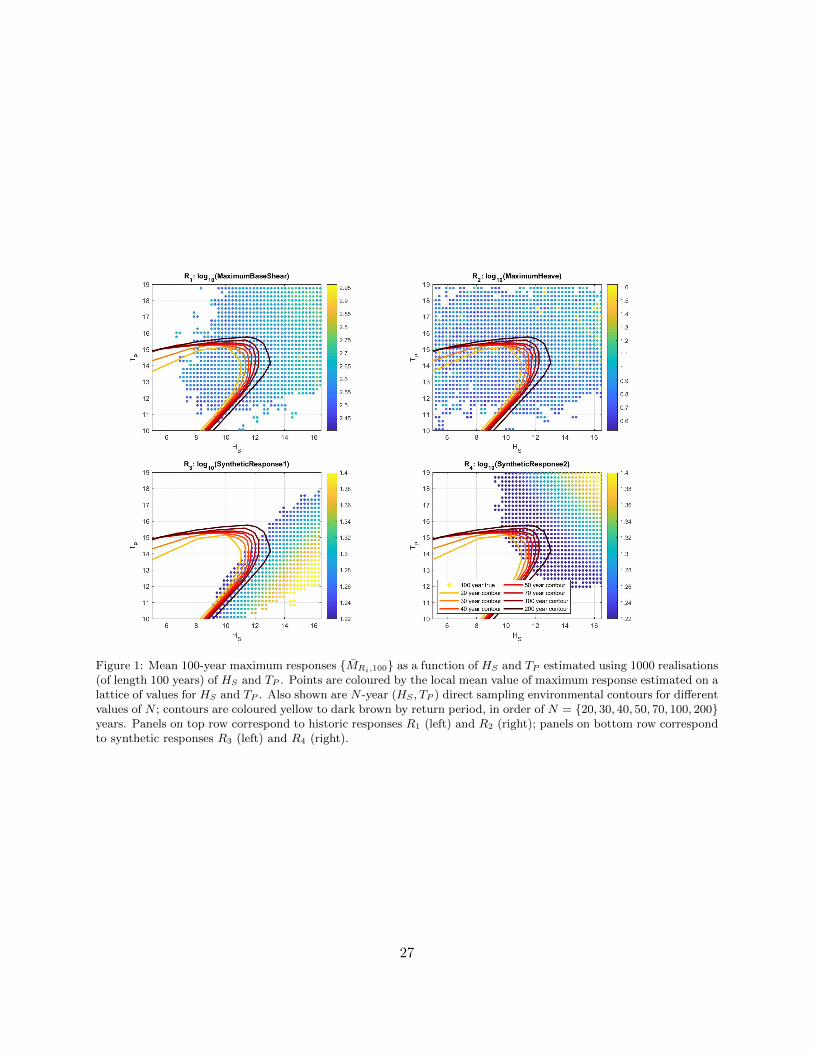
For each response in turn, the mean value M̄R,100 of the maximum 100-year response MR,100

is plotted in Figure 1, and coloured by the value of MR,100. Also plotted in the figure are directsampling contours corresponding to 20, 30, 40, 50, 70, 100 and 200 years. Note that for eachresponse Ri, only combinations of HS and TP giving rise to a least one occurrence of MRi,N appearin the figure.

[Figure 1 about here.]

The figure shows typical features of the different responses. Synthetic response R3 shows resonanceeffects TP ≈ 13s. Maximum base sheer (R1) and synthetic response R4 increase with increasingHS and TP . This is true in general for maximum heave (R2), but there are clearly large valuesof MR2,100 within even the 20-year environmental contour. That is, there are relatively benignenvironmental conditions, not even exceeding the 20-year contour, which sometimes generate the100-year maximum response. For contours to be useful, we would expect to see the largest valuesof 100-year maximum response lying outside the 100-year contour, and smallest values of responsewithin it. This is approximately the case for all responses, but certainly not always true for R2.

The extent to which the maximum response on the 100-year environmental contour agrees withthe actual distribution of MR,N from simulation can be assessed by comparing an estimate for thedistribution of the true response against that evaluated for conditions on the contour, as illustratedin Figure 2. It shows kernel density estimates for {MRi,100} estimated by direct simulation (indashed blue; which can be regarded as “the truth”). The figure also shows corresponding kerneldensity estimates for fMR,100Frontier of MR,100 from combinations of (HS , TP ) lying on the contourfrontier (scenario (b), shown in Figure 1), for a range of choices of N .

[Figure 2 about here.]

19

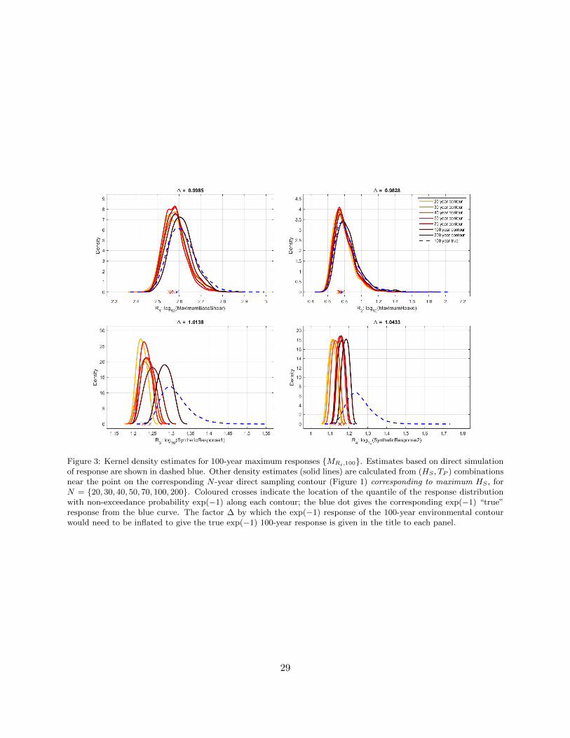
There is an obvious ordering of response density estimates with increasing return period, partic-ularly for responses R3 and R4 as might be expected. Further, the location of densities estimatedfrom different N -year environmental contours agrees to some degree with that of the true densityof MR,100. Moreover, for most cases the location of the quantile (see Section 4.6 with pC = pR)of the distribution of maximum response with non-exceedance probability exp(−1) (henceforth the“exp(−1)” value) of the density estimate from the 100-year environmental contour is in reasonableagreement with the location of the true exp(−1) value. Following Section 4.6, defining ∆ as theratio of the exp(−1) quantile of the true 100-year maximum response to the exp(−1) quantile ofthe distribution from the 100-year environmental contour, we see that the environmental contourapproach underestimates the exp(−1) response by between 1% and 9% for these examples.

We next perform a similar comparison of response distributions, this time using only (HS , TP )combinations near the point on the contour with maximum HS (that is, scenario (a), to estimatefMR,100Point). Results, shown in Figure 3, have similar general characteristics to those of Figure 2.Values of ∆ in the interval (0.98, 1.04) are estimated. In the current illustrations, therefore, itappears that both scenarios (a) and (b) provide reasonable estimates for the exp(−1) quantile ofMR,100.

[Figure 3 about here.]

5.2. Case study 2

Here we extend the study of Section 5.1 for responses R1 (maximum base shear) and R2 (max-imum heave), specifically to make a comparison of direct sampling contours, joint exceedance con-tours (Section 4.3.2), and isodensity contours (from a conditional extremes analysis in Section 3.4).For brevity, these approaches are henceforth referred to as “direct sampling”, “joint exceedance”and “empirical density” respectively in this section.

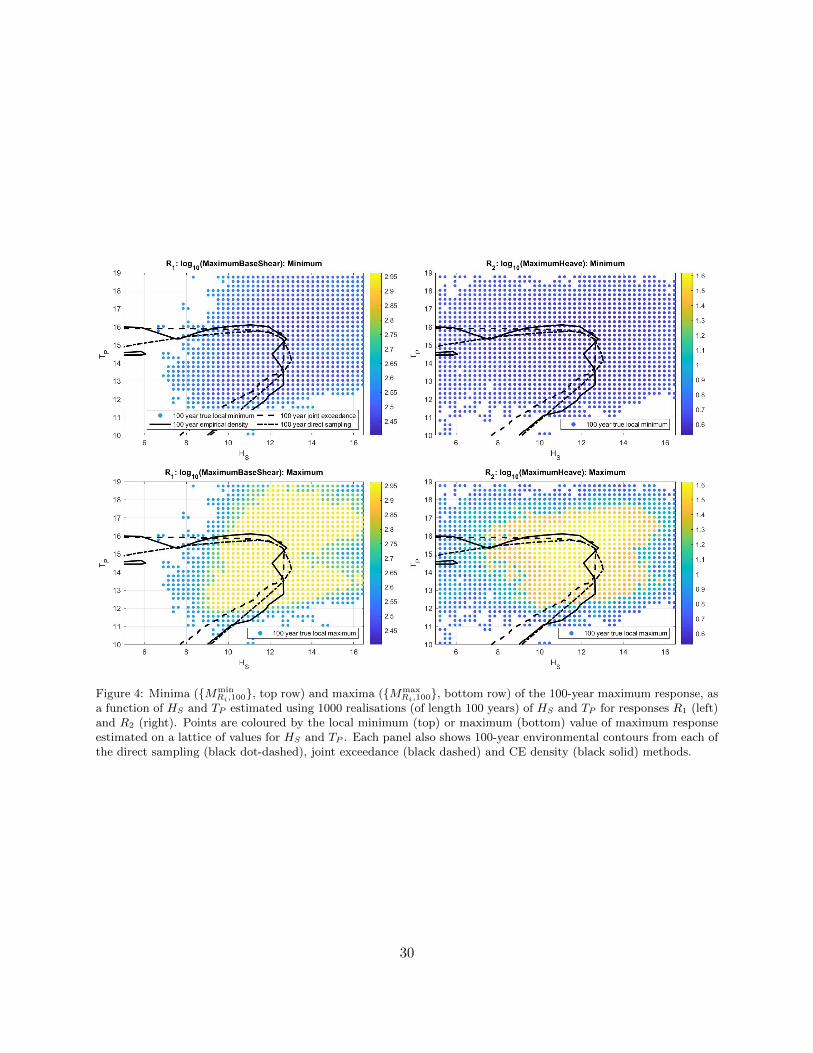
Figure 4 shows minima {MminRi,100

} and maxima {MmaxRi,100

} values of maximum responses {MRi,100}from the same 1000 simulations used to generate Figure 1. The colour of each disc in the top rowindicates the value of the minimum 100-year maximum response seen for that combination of HS

and TP , using the same algorithm as for Figure 1 to identify near neighbours. The bottom row showscorresponding values of maximum 100-year maximum response. It is clear that there is considerablevariability in response for a given pair of values for HS and TP . 100-year environmental contoursfrom each of the direct sampling, joint exceedance and empirical density methods are also shown inthe figure. All contours have a similar frontier interval. There is good agreement between the directsampling and joint exceedance contours in particular on the frontier interval; this is not surprisingsince the underlying methods have similar motivations. For the same simulation size, the empiricaldensity contour is more difficult to estimate without applying considerable smoothing. Comparingthe top and bottom rows of the figure, it also appears that the natural variability in the response(near the frontier interval of the contours) dominates any variability in the value of response alongthe contours. In this case, therefore, none of the contours is particularly preferable; any of themwould give approximately the same quality of estimate for MR,100.

It is interesting and intuitively appealing that the (yellow) area of largest values of maximumresponse (on the bottom row of the figure) is centred approximately on the frontier interval of thecontours. However, for synthetic response R3 in Figure 1, we see that the frontier interval is offset(to lower TP ) from part of the environmental contour corresponding to largest HS : focussing onan interval on the contour corresponding to largest HS to estimate MR,100 would seem particularlysuspect in this case, regardless of the choice of contour method.

20

Overall, it appears that the key to success is ensuring that the response is quantified (usingtime-domain simulation or other) at a sufficient number of (HS , TP ) combinations on or near thefrontier interval of any reasonably well-defined contour.

[Figure 4 about here.]

6. Discussion and conclusions

As shown in Section 4, environmental contours provide useful characterisations of the extent ofthe joint distribution of environmental variables. Some contour methods assume particular para-metric forms for the (conditional) distributions of environmental variables; other methods generateconvex contours on particular scales; other contour approaches are only defined on part of thedomain of environmental variables. There is concern in the user community that a contour should“look right”, closely hugging the boundaries of scatter plots of historic or simulated environmentalvariables.

The usual motivation for applying a contour approach in ocean engineering is to find environ-mental conditions efficiently (for a return period of N years say) which will generate approximatelythe N -year maximum response. Environmental contours therefore provide a means of reducing theburden of running full long-term response analysis for a wide range of environmental conditions.Different types of environmental contours find favour based on their ability to estimate the N -yearmaximum response from the N -year environmental contour.

An environmental contour is estimated with no regard whatsoever to structural details. Sinceenvironmental contours are independent of structural specifics, they can then be used in principle tostudy different structures in a given environment provided that the underlying assumptions linkingenvironment and structure are not violated.

There is no fundamental link between points on an environmental contour and structural re-sponse in general, and no reasonable expectation therefore that points on the N -year environmentalcontour should yield the N -year maximum response. Attempts have been made to compare differ-ent environmental contour methods using a response-based criterion, although it is mathematicallyobvious and generally recognised in the user community that no single approach is appropriatefor all structure and response types, and that considerable ambiguity will always remain. Themanner in which an environmental contour relates to extreme response depends on the specifics ofthe structure. However, for typical HS-driven structures, empirical evidence suggests the responsesgenerated from points along the environmental contour in (HS , TP )-space for a given return periodare reasonable estimates of the actual maximum response corresponding to the same return period.In the presence of resonant response and non-extreme values of TP , using points from the contournear the maximum HS can be misleading, since the response is not completely HS-dominated. Itis critical therefore that the dominant environmental variables are included in the estimation ofenvironmental contour. It is apparent from physical considerations that extreme occurrences ofsome structural responses should not coincide with those of extreme environmental variables; theN -year environmental contour is unlikely to provide any guidance regarding the N -year maximumresponse for such responses. We also note methods to adjust (or inflate) contours to correct forsources of bias (for estimation of extreme response) including the effects short-term variability, vi-olation of (marginal and dependence) modelling assumptions, uncertainty in parameter estimates,etc.

21

There is some debate within the user community regarding the relative merits of using ob-servations of the environmental variables for serially-dependent sea states, compared with near-independent storm peak characteristics. Given that the rates of occurrence of events are taken intoaccount, both can provide useful estimates of joint models for the environment and hence environ-mental contours. The advantage of using sea state data is that sample size is large, potentiallyallowing a more detailed description of the joint distribution of environmental parameters to beestimated. However, because sea state data is serially-correlated, naive estimates of uncertaintiesfor model parameters and inferences under the model will be too small, but can be corrected (forexample, using sandwich estimators or bootstrap resampling).

Multi-modal distributions of environmental variables can be caused by different physical pro-cesses or by covariate effects (for example, fetch length as a function of direction); in these cases,isodensity contours may be more reasonable summaries of the joint distribution than those basedon joint exceedance, since there may be regions of low probability between modes. Further itmay be useful to partition the environmental space by covariate and perform separate analyses perpartition. Alternatively, it is also possible to estimate joint models incorporating covariate effects.

Basing design conditions on the N -year environmental contour alone neglects sources of biasand variability in estimation of the N -year maximum response, including short-term variability inresponse. Approximate methods to inflate the environmental contour, or adjust its return period,are available. It is always possible, given fully-specified environments and structural responses,to estimate inflation factors which map some quantile of the distribution of N -year maximumresponse onto the corresponding quantile of the distribution of maximum response given sea stateson the environmental contour. However, the value of inflation factor in general will be a functionof quantile level, the structure and the response. It is likely that estimating inflation factors (oradjusting contour return periods) based on comparing central characteristics (for example, mean,median or mode) of response distributions will prove more stable, since Monte Carlo simulationsof a given size provide better estimates of central characteristics than those of tails.

In some applications, it may be that environmental contours will be used to estimate multiplecorrelated responses. In such cases, care needs to be taken that the contour is used to estimatethe responses jointly corresponding to a given return period, rather than estimating independentmarginal return values.

As can be seen from the end-user survey in Appendix A.1, there are valid concerns regardinga sensible definition of an environmental contour, its estimation and adjustment in relation tostructural response. There are many articles in the literature comparing different contour methods,inflation factors etc. However, in reality, most sensibly-proposed contour methods (including thedirect sampling, joint exceedance and empirical density examined here) locate the frontier intervalof the contour within the same region of environmental space. Uncertainties due to the detailsof the structure, and even when the structure is defined to the natural variability of structuralresponse given the environment, are in general issues of far greater concern. Any reasonable choiceof contour, given the considerations explored in this paper, will suffice.

Methods such as IFORM and the direct sampling method are advantageous in that they imposea link between environment and structure by make assumptions about the characteristics of fail-ure surfaces as a function of the environmental variables. Given these assumptions, it is possibleto link the exceedance probability associated with a given environmental contour with structuralfailure probability. Although conditions from an N -year environmental contour need not resultexactly in N -year responses, IFORM and direct sampling provide at least some understanding of

22

how an N -year environmental contour is related to the N -year maximum response. Both IFORMand direct sampling approaches assume a linearised failure boundary. The basic difference betweenthe approaches arises from the fact that linearisation for IFORM is performed in the transformedU -space, and in direct sampling approach in the original X-space of environmental variables (e.g.Vanem and Bitner-Gregersen 2015; Vanem 2017 and references therein). For both IFORM anddirect sampling contours, the relationship established is between the exceedance probability asso-ciated with the contour (on some scale) and the probability of structural failure. This does notguarantee however that searching along an IFORM or direct sampling contour for return period Twill isolate the key features of the T -year maximum response; the relative performance of IFORMand direct sampling in estimating extreme responses is application-dependent.

For better specification of design conditions, a response model is necessary. To determine thefrontier interval of a design contour within the domain of environmental variables, inflation factorsfor contours etc., some knowledge of, or working assumption regarding the response is required.As specification of the response evolves, sufficient, for example, to estimate the frontier intervaland inflation factors, arguably there is already sufficient information (or supposition) to use bettermodels to describe approximate responses and their uncertainties. From a statistical perspective,it is hard to avoid the impression that, in terms of estimating extreme structural response, anenvironmental contour is just an approximation to a sample from the tail of the distribution ofenvironmental variables. In fact, for most purposes, an appropriate sample from the tail of thedistribution of environmental variables would be preferable. Furthermore, with the advent ofmethods such as statistical emulation (used widely in approximating complex physical systems,including metocean design e.g. Gouldby et al. 2014; Jones et al. 2018), a computationally-efficientapproximate response model can be estimated, along with its uncertainty, for many if not allapplications. Given this, the emulator would provide a mechanism for response-based design inall situations, avoiding the need for environmental contours completely. It is apparent that thecoastal engineering community is already moving in this direction (e.g. Gouldby et al. 2017); a keyassumption with statistical emulation is that a representative set of cases is available to quantifyall important relationships between environment and structural loading. Nevertheless, part of theuser-cited strength of the environmental contour method is its relative simplicity and computationalefficiency. There is clearly a trade-off between a thorough probabilistic response-driven analysis(which may be technically more involved and less familiar to the practitioner) compared to asimple approximate approach (with which the user is relatively familiar and confident).

Given the above considerations, and comments in the end-user survey, to assist the practitionerin deciding when and where to use an environmental contour approach, we present the followingbrief check-list. We recommend the use of environmental contours in the following circumstances.

6.1. When to use environmental contours

• Nature of responses and environmental variables are known: The dominant struc-tural responses are all known. The dominant environmental variables driving each structuralresponse are all known, and the value of response is dominated by long-term variability of theenvironmental variables: extreme environments produce extreme responses. The influenceof short-term environmental variability is relatively small. [There are some responses (forexample, fatigue) that are not dominated by extremes of the environment; environmentalcontour methods are therefore not appropriate.]

• Response-based analysis is not possible: (a) There are no adequate computationally-

23

efficient structural response models available. [If these models are available, a response-basedanalysis should be performed.] (b) There are computationally-demanding structural responsemodels available, but no time or expertise to develop approximate structural response models(for example, generic load models, statistical emulators) using these. [If these models can beestimated, a response-based analysis should be performed.]

• At outline design stage: The specifics of the structure may not be clear at outline design.For this reason, the environmental contour may provide a useful source of extreme sea statessuitable for evaluating a range of different structures.

Once it has been decided that an environmental contour approach is suitable, the following arethen recommended.

6.2. How to use environmental contours wisely

• Reality check: Remember that environmental contours are approximate methods that canonly provide approximations to extreme responses. The use of contour approaches may needto be supported in final design by full long-term analysis.

• Sufficient environmental data available: There are sufficient historical data availableto estimate the joint distribution of all these environmental variables adequately using, forexample, a method from Section 3.

• Estimate more than one environmental model, and consider the sensitivity of themodel to arbitrary modelling choices: The sensitivity of environmental contour estimatesto arbitrary choices made when estimating a model for the joint distribution of environmentalparameters should be investigated. [When different equally-plausible environmental modelsprovide different contour estimates, the current research suggests that all contours shouldbe considered valid and used together for choice of environmental values corresponding toextreme responses. Equally, the user might well be concerned when two different environ-mental models provide materially different contour estimates (using a common contouringapproach).]

• If unsure which contour to use, estimate more than one type: Each type of en-vironmental contour is seeking to achieve different objectives. If you are not clear whichcontour is most suitable for your application, consider estimating contours of different types,and establish approximate consistency of inferences from different contours. [When differentequally-plausible contours give materially different results, all contours should be consid-ered valid and used together for choice of environmental values corresponding to extremeresponses.]

• Choose multiple points from the environmental contours for response evaluation:Multiple combinations of values of environmental variables falling on or near the frontierinterval of the environmental contour should be used. [When the frontier interval is not known,a wide set of combinations of values of environmental variables on or near the environmentalcontour should be used. If in doubt, choose more points and choose points more widely.]

• Consider other sources of uncertainty: (a) How influential are the effects of covari-ates (directionality, seasonality) [If important, fit a non-stationary environmental model (for

24

example, using PPC from Section 5)]; (b) Have all environmental variables influencing the re-sponse been considered in the environmental model and contours? [If not, consider estimatingenvironmental models and contours in higher dimensions].

7. Acknowledgement

This work was part-funded by the European Union ERA-NET project entitled “EnvironmentalContours for SAfe DEsign of Ships and other marine structures (ECSADES)”. The PPC softwareand user guide is freely-available as MATLAB code from the authors. We thanks Kevin Ewans foruseful comments on the manuscript.

25

List of Figures

1 Mean 100-year maximum responses {M̄Ri,100} as a function of HS and TP estimatedusing 1000 realisations (of length 100 years) of HS and TP . Points are coloured bythe local mean value of maximum response estimated on a lattice of values for HS

and TP . Also shown are N -year (HS , TP ) direct sampling environmental contours fordifferent values of N ; contours are coloured yellow to dark brown by return period,in order of N = {20, 30, 40, 50, 70, 100, 200} years. Panels on top row correspondto historic responses R1 (left) and R2 (right); panels on bottom row correspond tosynthetic responses R3 (left) and R4 (right). . . . . . . . . . . . . . . . . . . . . . . . 27

2 Kernel density estimates for 100-year maximum responses {MRi,100}. Estimatesbased on direct simulation of response are shown in dashed blue. Other density es-timates (solid lines) are calculated from (HS , TP ) combinations lying near the corre-spondingN -year direct sampling contour shown in Figure 1, forN = {20, 30, 40, 50, 70, 100, 200}.Coloured crosses indicate the location of the quantile of the response distribution withnon-exceedance probability exp(−1) along each contour; the blue dot gives the cor-responding exp(−1) “true” response from the blue curve. The factor ∆ by which theexp(−1) response of the 100-year environmental contour would need to be inflatedto give the true exp(−1) 100-year response is given in the title to each panel. . . . . 28

3 Kernel density estimates for 100-year maximum responses {MRi,100}. Estimatesbased on direct simulation of response are shown in dashed blue. Other densityestimates (solid lines) are calculated from (HS , TP ) combinations near the pointon the corresponding N -year direct sampling contour (Figure 1) corresponding tomaximum HS , for N = {20, 30, 40, 50, 70, 100, 200}. Coloured crosses indicate thelocation of the quantile of the response distribution with non-exceedance probabilityexp(−1) along each contour; the blue dot gives the corresponding exp(−1) “true”response from the blue curve. The factor ∆ by which the exp(−1) response of the100-year environmental contour would need to be inflated to give the true exp(−1)100-year response is given in the title to each panel. . . . . . . . . . . . . . . . . . . 29

4 Minima ({MminRi,100

}, top row) and maxima ({MmaxRi,100

}, bottom row) of the 100-yearmaximum response, as a function of HS and TP estimated using 1000 realisations(of length 100 years) of HS and TP for responses R1 (left) and R2 (right). Pointsare coloured by the local minimum (top) or maximum (bottom) value of maximumresponse estimated on a lattice of values for HS and TP . Each panel also shows 100-year environmental contours from each of the direct sampling (black dot-dashed),joint exceedance (black dashed) and CE density (black solid) methods. . . . . . . . . 30

26

Figure 1: Mean 100-year maximum responses {M̄Ri,100} as a function of HS and TP estimated using 1000 realisations(of length 100 years) of HS and TP . Points are coloured by the local mean value of maximum response estimated on alattice of values for HS and TP . Also shown are N -year (HS , TP ) direct sampling environmental contours for differentvalues of N ; contours are coloured yellow to dark brown by return period, in order of N = {20, 30, 40, 50, 70, 100, 200}years. Panels on top row correspond to historic responses R1 (left) and R2 (right); panels on bottom row correspondto synthetic responses R3 (left) and R4 (right).

27

Figure 2: Kernel density estimates for 100-year maximum responses {MRi,100}. Estimates based on direct simulationof response are shown in dashed blue. Other density estimates (solid lines) are calculated from (HS , TP ) combinationslying near the corresponding N -year direct sampling contour shown in Figure 1, for N = {20, 30, 40, 50, 70, 100, 200}.Coloured crosses indicate the location of the quantile of the response distribution with non-exceedance probabilityexp(−1) along each contour; the blue dot gives the corresponding exp(−1) “true” response from the blue curve. Thefactor ∆ by which the exp(−1) response of the 100-year environmental contour would need to be inflated to give thetrue exp(−1) 100-year response is given in the title to each panel.

28

Figure 3: Kernel density estimates for 100-year maximum responses {MRi,100}. Estimates based on direct simulationof response are shown in dashed blue. Other density estimates (solid lines) are calculated from (HS , TP ) combinationsnear the point on the corresponding N -year direct sampling contour (Figure 1) corresponding to maximum HS , forN = {20, 30, 40, 50, 70, 100, 200}. Coloured crosses indicate the location of the quantile of the response distributionwith non-exceedance probability exp(−1) along each contour; the blue dot gives the corresponding exp(−1) “true”response from the blue curve. The factor ∆ by which the exp(−1) response of the 100-year environmental contourwould need to be inflated to give the true exp(−1) 100-year response is given in the title to each panel.

29

Figure 4: Minima ({MminRi,100

}, top row) and maxima ({MmaxRi,100

}, bottom row) of the 100-year maximum response, asa function of HS and TP estimated using 1000 realisations (of length 100 years) of HS and TP for responses R1 (left)and R2 (right). Points are coloured by the local minimum (top) or maximum (bottom) value of maximum responseestimated on a lattice of values for HS and TP . Each panel also shows 100-year environmental contours from each ofthe direct sampling (black dot-dashed), joint exceedance (black dashed) and CE density (black solid) methods.

30

Appendix A. Supporting information

Appendix A.1. Survey findings

Further details of the survey summarised in Section 1.3 are given here. For brevity, the respon-dents full answers are summarised here. The full (anonymised) survey responses can however beprovided on request.

The survey questions were distributed to industry/consulting contacts of those involved in theECSADES project as well as authors of key literature in the area. We do not claim that thissample is representative of the user community for contours, but hopefully it is informative. Ofthe 19 respondents, a large number were based in Norway with contributions also from the US, theNetherlands, the UK and Australia; with 7 from academia and 12 from industry/consulting.

1. How many times have you used environmental contours as part of your work in the last 3years?

• Different frequencies of use: from daily to hardly ever

• Geographic variability: frequent use cited by respondents based in Norway, less frequentin the U.S.

• Contours form an integral part of reliability assessment / design practices

• Academically, contours garner less interest. Appearing mainly in post-graduate projectswith industrial applications.

2. What kind of environmental contours do you use (for example, derived from FORM, or theconditional extremes model of Heffernan & Tawn, or other)?

• Large user group for FORM/IFORM

• Conditional extremes approach of Heffernan and Tawn (2004)

• Marginal and dependence modelling based on threshold exceedance distributions

• AND and JOIN-SEA cited for coastal applications

• Kernel density estimation

• The need for contours in any form also questioned in the event that direct response-basedanalysis is possible

3. For what purpose do you use environmental contours? Can you describe as precisely aspossible the information you take from the environmental contour, and how you use this? Doyou use the whole contour or just part of it? Which part of the contour, and why? Do youactually need information about the whole contour? Do you take any steps to account foruncertainties and potential biases?

• Two dimensional contour representing “N-year” environmental conditions is typicallyestimated (never higher dimensions)

• Response analysis performed on a subset of points along the environmental contour

• Region of the contour over which this subset of points is focussed can be motivated byphysical understanding of mechanisms driving response, for example, wave-dominatedor resonant response

• Sometimes only “short term” response analysis performed; additional extrapolation from“short-term” to “long-term” necessary.

31

• N-year structural response is estimated from the responses resulting from conditionsdefined by points on the environmental contour by:

– Inflating the response somehow: 90% quantile, median× 1.3 or other ad-hoc method,to adjust for short-term variability

– Inflate environment: that is, explore responses for a contour representing a longerreturn period (N)

• Bias, (epistemic) uncertainty and inherent (aleatory) randomness is almost never incor-porated

4. What do you think are the advantages of using environmental contours?

• Environmental contours provide a reasonable approximate approach to estimate N-yearresponses

• Industry-accepted

• Calculated without any knowledge of structure being designed; independent of the re-sponse; same contour can be used for range of responses

• Simple to use, inexpensive, quick - especially for typical cases (for example, Hs-Tp)

• Computational efficiency compared full time-domain analysis

5. What, in your opinion, are the disadvantages or problems associated with using environmentalcontours? Are there specific circumstances in which you find that environmental contours donot work well or are difficult to use?

• Concern about details of choosing response from a subset estimated along the contour:using arbitrary quantiles and scale factors etc.

• Simulations using short-term responses used to estimate long-term response; high quan-tile necessary.

• Environmental contour method does not involve the response directly (so arbitrary cal-ibration of response will always be necessary); response-based analysis is a better ap-proach when possible

• Clients do not understand what the contour represents and how it has been calculated,can therefore sometimes be a hard sell

• Lots of approaches to defining the contour, not clear which (if any) is better

• Nave application of statistical methods can yield physically unreasonable contours (forexample, non-physical wave steepness)

• Approaches to extending to higher dimensions (3D and above) or to multiple responsesare more ad-hoc, incorporating correct physics even more problematic

• Need to check conclusions using full-scale simulation / long-term analysis

• No obvious way to estimate the distributional properties of N-year response

• Uncertainties are rarely quantified

6. Do you use design guidelines or other literature sources to guide your use of environmentalcontours? Could you list these?

• Statoil procedures

32

• Norsok N003

• DNV-RP-C205 (2014)

• FORM/iFORM: Winterstein et al. (1993)

• JOIN-SEA: Hawkes et al. (2002)

• Heffernan and Tawn (2004)

• Shell LSM model for response-based design

Appendix A.2. PPC model

The penalised piecewise constant (PPC) extreme value model allows the estimation of non-stationary marginal and conditional extremes for peaks over threshold using a simple description ofnon-stationarity with respect to covariates in marginal and dependence models. An early deploy-ment of the PPC model as software is described in Ross et al. (2018); the current version of the PPC

software, developed as part of the ECSADES project (see Section 7), is freely available from theauthors. For each observation xi in the sample {xi}, we assume that an associated (potentially vec-tor) covariate θi is available. The value of covariate θi is used to allocate the observation to one andonly one of nC covariate intervals {Ck}nC

k=1 by means of an allocation vector A such that k = A(i)and {xi} =

⋃Ck. For each k, all observations in the set {xi′}A(i′)=k with the same covariate

interval Ck are assumed to have common extreme marginal and dependence characteristics.Non-stationary marginal extreme value characteristics of each variate Xj are then estimated in

turn using a generalised Pareto model and cross-validated roughness-penalised maximum likelihoodestimation. For variable Xj and covariate interval Ck, the extreme value threshold ψjk > 0 isassumed to be a quantile of the empirical distribution of the variate in that interval, with specifiednon-exceedance probability τj ∈ (0, 1), with τj constant across intervals, and estimated by counting.Threshold exceedances are assumed to follow the generalised Pareto distribution with shape ξj ∈ Rand scale σjk > 0. ξj is assumed constant (but unknown) across covariate intervals, and thereasonableness of the assumption assessed by inspection of diagnostic plots. Parameters ξj , {σjk}are estimated by maximising the predictive performance of a roughness-penalised model, optimallyregulating the extent to which {σjk} varies across interval, using a cross-validation procedure.

After marginal fitting, the sample {xi} is transformed to standard Laplace scale as {x̃i} and theconditional extremes model outlined in Section 3.4 fitted. Following the notation of that section,for each choice of conditioning variate Xq, linear parameters α−q for the conditioned variatesvary across covariate bins with variation regularised using cross-validation to optimise predictiveperformance for each response in turn. The corresponding value of exponent parameters β−k isassumed constant with respect to covariates. Sets of residuals R−q from the fit, for each choice ofq are also isolated.

Simulation under the fitted model, and transformation of realisations to their original marginalscale is then possible, corresponding to a return period of arbitrary length. In particular, samplessimulated under the model can be used to estimate environmental contours of different types, andexplore their relative characteristics. In practice, the full PPC modelling procedure is repeated for nUbootstrap resamples of the original sample to capture sampling uncertainty, each resample using adifferent choice of marginal and dependence thresholds to capture threshold uncertainty. Estimatesfor marginal and dependence parameters therefore correspond to nU arrays of values capturingsampling and threshold specification uncertainty, which are used to propagate uncertainty fromthese sources into simulations under the model.

33

We use the PPC model to estimate a number of the environmental contours discussed in Sec-tion 4 and investigate their characteristics, in particular their relationship to extremes of structuralresponse. Specifically, because of its recently popularity, we consider the direct sampling contour(Section 4.3.1); we also consider the joint exceedance contour outlined in Section 4.3.2. Both thesecontour methods use a simulated sample under the environmental model as starting point. Furtherwe consider an isodensity contour (Section 4.4 based on the conditional extremes model of Sec-tion 3.4; this approach infers the contour directly from the properties of the environmental modelwith no need for simulation.

34

References

Barber, D., 2012. Bayesian reasoning and machine learning. Cambridge University Press.

Bender, J., Wahl, T., Jensen, J., 2014. Multivariate design in the presence of non-stationarity.Journal of Hydrology 514, 123–130.

Bitner-Gregersen, E. M., 2015. Joint met-ocean description for design and operations of marinestructures. Appl. Ocean Res. 51, 279–292.

Bitner-Gregersen, E. M., Haver, S., 1989. Joint long term description of environmental parametersfor structural response calculations. In: Proc. 2nd international workshop on wave hindcastingand forecasting.

Bitner-Gregersen, E. M., Haver, S., 1991. Joint environmental model for reliability calculations. In:Proc. ISOPE 91, pp. 246-253.

Chai, W., Leira, B. J., 2018a. Environmental contours based on inverse SORM. Marine Structures60, 34–51.

Chai, W., Leira, B. J., 2018b. Environmental contours based on inverse sorm. Marine Structures60.

CIRIA, 1996. Beach Management Manual. ISBN 0-860174387.

CIRIA, 2007. The Rock Manual. The use of rock in hydraulic engineering (2nd edition). ISBN978-0-86017-683-1.

Coles, S., 2001. An introduction to statistical modelling of extreme values. Springer.

Coles, S., Heffernan, J., Tawn, J., 1999. Dependence measures for extreme value analyses. Extremes2, 339–365.

Coles, S., Tawn, J., 1990. Statistics of coastal flood prevention. Philos. T. Roy. Soc. A 332, 457–476.

Dahl, K. R., Huseby, A. B., 2018. Buffered environmental contours. In: Safety and Reliability - SafeSocieties in a Changing World: Proceedings of the European safety and reliability Conference.

DEFRA / Environment Agency, 2003. Joint probability: dependence mapping and best practice.UK DEFRA / Environment Agency, Flood and Coastal Defence R&D Programme.

DEFRA / Environment Agency, 2005. Use of Joint Probability Methods in Flood Management AGuide to Best Practice. UK DEFRA / Environment Agency, Flood and Coastal Defence R&DProgramme.

DNV-RP-C205, 2010. Environmental conditions and environmental loads. Det Norske Veritas.

DNVGL-RP-C205, 2017. Environmental conditions and environmental loads. Det Norske Veritasgroup, Norway.

Durante, F., Salvadori, G., 2009. On the construction of multivariate extreme value models viacopulas. Environmetrics 21, 143–161.

35

E&P Forum, 1985. The application of joint probabilities of metocean phenomena in the oil indus-try’s structural design work. In: Workshop, London.

Ewans, K. C., Jonathan, P., 2008. The effect of directionality on northern North Sea extreme wavedesign criteria. J. Offshore. Arct. Eng. 130, 041604:1–041604:8.

Fazeres-Ferradosa, T., Taveira-Pinto, F., Vanem, E., Reis, M. T., das Neves, L., 2018. Asymmetriccopula-based distribution models for met-ocean data in offshore wind engineering applications.Wind Engineering 42, 304–334.

Feld, G., Randell, D., Ross, E., Jonathan, P., 2018. Design conditions for waves and water lev-els using extreme value analysis with covariates. (Submitted to Ocean Engineering, draft atwww.lancs.ac.uk/∼jonathan).

Francois, M., Camps, C., Alvarez, J., Quiniou, V., 2007. Multi-variate i-form contours for thedesign of offshore structures (practical methodology and application to a west africa fpso). In:Proc. 17th International Offshore and Polar Engineering Conference, Lisbon, Portugal.

Gouldby, B., Mendez, F., Guanche, Y., Rueda, A., Minguez, R., 2014. A methodology for derivingextreme nearshore sea conditions for structural design and flood risk analysis. Coastal Eng. 88,15–26.

Gouldby, B., Wyncoll, D., Panzeri, M., Franklin, M., Hunt, T., Hames, D., Tozer, N., Hawkes, P.,Dornbusch, U., Pullen, T., 2017. Multivariate extreme value modelling of sea conditions aroundthe coast of england. Proceedings of the Institution of Civil Engineers - Maritime Engineering170, 3–20.

Gudendorf, G., Segers, J., 2010. Copula theory and its applications. Lecture Notes in Statistics198. Edts. Jaworski P., Durante F., Hrdle W., Rychlik T. Springer, Berlin, Heidelberg, Ch.Extreme-value copulas.

Haselsteiner, A. F., Ohlendorf, J.-H., Wosniok, W., Thoben, K.-D., 2017. Deriving environmentalcontours from highest density regions. Coastal Eng. 123, 42–51.

Haver, S., 1987. On the joint distribution of heights and periods of sea waves. Ocean Eng. 14,359–376.

Haver, S., Winterstein, S., 2009. Environmental contour lines: a method for estimating long termextremes by a short term analysis. Trans. Soc. Nav. Archit. Mar. Eng. 116, 116–127.

Hawkes, P. J., Gouldby, B. P., Tawn, J. A., Owen, M. W., 2002. The joint probability of waves andwater levels in coastal defence design. Journal of Hydraulic Research 40, 241–251.

Heffernan, J. E., Resnick, S. I., 2007. Limit laws for random vectors with an extreme component.Ann. Appl. Probab. 17, 537–571.

Heffernan, J. E., Tawn, J. A., 2004. A conditional approach for multivariate extreme values. J. R.Statist. Soc. B 66, 497–546.

Horn, J.-T., Bitner-Gregersen, E., Krokstad, J. R., Leira, B. J., Amdahl, J., 2018. A new combi-nation of conditional environmental distributions. Applied Ocean Research 73, 17 – 26.

36

HR Wallingford, 1998. The joint probability of waves and water levels: JOIN-SEA, A rigorous butpractical new approach. HR Wallingford (Report SR 537).

Huseby, A., Vanem, E., Natvig, B., 2015a. Alternative environmental contours for structural relia-bility analysis. Struct. Saf. 54, 32–45.

Huseby, A. B., Vanem, E., Eskeland, K., 2017. Evaluating properties of environmental contours.In: Safety and Reliability, Theory and Applications: Proceedings of the European safety andreliability Conference.

Huseby, A. B., Vanem, E., Natvig, B., 2013. A new approach to environmental contours for oceanengineering applications based on direct monte carlo simulations. Ocean Eng. 60, 125–135.

Huseby, A. B., Vanem, E., Natvig, B., 2015b. A new Monte Carlo method for environmental contourestimation. In: Safety and Reliability, Theory and Applications: Proceedings of the Europeansafety and reliability Conference.

IACS, 2001. Standard wave data for direct wave load analysis. International Association of Classi-fication Societies, UK.

IMO, 2001. Guidelines for formal safety assessment for the IMO rule making process (Marine SafetyCommittee 74/WP.19). International Maritime Organisation.

ISO19901-1, 2015. Petroleum and natural gas industries. Specific requirements for offshore struc-tures. Part 1: Metocean design and operating considerations. First edition. International Stan-dards Organisation.

Jaworski, P., Durante, F., Hrdle, W., Rychlik, T. e., 2010. Copula theory and its applications.Lecture Notes in Statistics 198. Springer, Berlin, Heidelberg.

Jonathan, P., Ewans, K., Flynn, J., 2014a. On the estimation of ocean engineering design contours.ASME J. Offshore Mech. Arct. Eng. 136:041101.

Jonathan, P., Ewans, K. C., 2007. The effect of directionality on extreme wave design criteria.Ocean Eng. 34, 1977–1994.

Jonathan, P., Ewans, K. C., Forristall, G. Z., 2008. Statistical estimation of extreme ocean envi-ronments: The requirement for modelling directionality and other covariate effects. Ocean Eng.35, 1211–1225.

Jonathan, P., Ewans, K. C., Randell, D., 2014b. Non-stationary conditional extremes of northernNorth Sea storm characteristics. Environmetrics 25, 172–188.

Jonathan, P., Flynn, J., Ewans, K. C., 2010. Joint modelling of wave spectral parameters forextreme sea states. Ocean Eng. 37, 1070–1080.

Jones, M. J., Hansen, H. F., Zeeberg, A. R., Randell, D., Jonathan, P., 2018. Uncertainty quantifi-cation in estimation of ocean environmental return values. (Accepted by Coastal Eng. in July,draft at www.lancs.ac.uk/∼jonathan).

Jordan, M. I., 2004. Graphical models. Stat. Sci. 19, 140–155.

37

Keef, C., Papastathopoulos, I., Tawn, J. A., 2013. Estimation of the conditional distribution of avector variable given that one of its components is large: additional constraints for the Heffernanand Tawn model. J. Mult. Anal. 115, 396–404.

Leira, B. J., 2008. A comparison of stochastic process models for definition of design contours.Structural Safety 30, 493 – 505.

Lutes, L., Winterstein, S., 2014. Design contours for load combinations: generalizing inverse formmethods to dynamic problems. In: Proceedings, 7th Computational Stochastic Mechanics Con-ference, Santorini.

Madsen, H. O., Krenk, S., Lind, N. C., 1986. Methods of structural safety. Englewood Cliffs:Prentice-Hall.

Mathisen, J., Bitner-Gregersen, E., 1990. Joint distributions for significant wave height and wavezero-up-crossing period. Applied Ocean Research 12, 93–103.

Montes-Iturrizaga, R., Heredia-Zavoni, E., 2015. Environmental contours using copulas. AppliedOcean Research 52, 125 – 139.

Montes-Iturrizaga, R., Heredia-Zavoni, E., 2016. Multivariate environmental contours using c-vinecopulas. Ocean Engineering 118, 68 – 82.

Montes-Iturrizaga, R., Heredia-Zavoni, E., 2017. Assessment of uncertainty in environmental con-tours due to parametric uncertainty in models of the dependence structure between metoceanvariables. Applied Ocean Research 64, 86 – 104.

Morison, J. R., O’Brien, M. P., Johnson, J. W., Schaaf, S. A., 1950. The force exerted by surfacewaves on piles. AIME Petrol. Trans. 189, 149–154.

Nelsen, R., 2006. An introduction to copulas. Springer.

NORSOK N-003, 2017. NORSOK Standard N-003:2017: Actions and action effects. NORSOK,Norway.

Papastathopoulos, I., Strokorb, K., Butler, A., Tawn, J., 2017. Extreme events of markov chains.J. Appl. Probab. 49, 134–161.

Reistad, M., Breivik, O., Haakenstad, H., Aarnes, O. J., Furevik, B. R., Bidlot, J.-R., 2011. A high-resolution hindcast of wind and waves for the North sea, the Norwegian sea, and the Barentssea. J. Geophys. Res. 116, 1–18.

Ribatet, M., Mohammed, S., 2012. Extreme value copulas and max-stable processes. Journal de laSocit Franaise de Statistique 153, 138–150.

Ross, E., Sam, S., Randell, D., Feld, G., Jonathan, P., 2018. Estimating surge in extreme NorthSea storms. Ocean Eng. 154, 430–444.

Serafin, K. A., Ruggiero, P., 2014. Simulating extreme total water levels using a time-dependent,extreme value approach. Journal Geophys. Res. - Oceans 119 (9), 6305–6329.

38

Serinaldi, F., 2015. Dismissing return periods! Stoch. Env. Res. Risk A. 29, 1179–1189.

Shooter, R., Ross, E., Tawn, J. A., Jonathan, P., 2018. On spatial conditional extremes for oceanstorm severity. In preparation for Environmetrics.

Tawn, J. A., 1992. Estimating probabilities of extreme sea levels. J. Roy. Statist. Soc. C 41, 77–93.

Tendijck, S., Ross, E., Randell, D., Jonathan, P., 2018. A non-stationary statisticalmodel for the evolution of extreme storm events. (Accepted by Environmetrics, draft atwww.lancs.ac.uk/∼jonathan).

Tromans, P. S., Vanderschuren, L., 1995. Variable based design conditions in the North Sea: ap-plication of a new method. Offshore Technology Confernence, Houston (OTC–7683).

Vanem, E., 2016. Joint statistical models for significant wave height and wave period in a changingclimate. Mar. Struct. 49, 180–205.

Vanem, E., 2017. A comparison study on the estimation of extreme structural response from dif-ferent environmental contour methods. Mar. Struct. 56, 137–162.

Vanem, E., 2018. 3-dimensional environmental contours based on a direct sampling method forstructural reliability analysis of ships and offshore structures. Ships and Offshore Structures,1–12.

Vanem, E., Bitner-Gregersen, E. M., 2015. Alternative environmental contours for marine structuraldesign - a comparison study. J. Offshore Mech. Arct. Eng. 137, 051601:1–8.

Winter, H. C., Tawn, J. A., 2016. Modelling heatwaves in central France: a case-study in extremaldependence. J. Roy. Statist. Soc. C 65, 345–365.

Winterstein, S., 2015. (unpublished manuscript) environmental contours: Including the effects ofdirectionality and other sub-populations.URL sites.google.com/site/probabilitybasedengineering/pbe-publications

(accessed 28.09.2018)

Winterstein, S., Engebretsen, K., 1998. Reliability-based prediction of design loads and variables forfloating ocean structures. In: Proc. 27th International Conf. on Offshore Mechanics and ArcticEngineering, Lisbon, Portugal.

Winterstein, S. R., Ude, T. C., Cornell, C. A., Bjerager, P., Haver, S., 1993. Environmental pa-rameters for extreme variable: Inverse Form with omission factors. In: Proc. 6th Int. Conf. onStructural Safety and Reliability, Innsbruck, Austria.

Yu, H., Dauwels, J., Jonathan, P., 2014. Extreme value graphical models with multivariate copulas.IEEE Transactions on Signal Processing 62, 5734–5747.

39