On Explaining Integer Vectors by Few Homogeneous Segments ✩ Robert Bredereck a,1 , Jiehua Chen a,2 , Sepp Hartung a , Christian Komusiewicz a , Rolf Niedermeier a , Ondˇ rej Such´ y b,3 a Institut f¨ ur Softwaretechnik und Theoretische Informatik, TU Berlin, Germany b Faculty of Information Technology, Czech Technical University in Prague, Czech Republic Abstract We extend previous studies on “explaining” a nonnegative integer vector by sums of few homogeneous segments, that is, vectors where all nonzero entries are equal and consecutive. We study two NP-complete variants which are motivated by radiation therapy and database applications. In Vector Positive Explanation, the segments may have only positive integer entries; in Vector Explanation, the segments may have arbitrary integer entries. Considering several natural parameterizations such as the maximum vector entry γ and the maximum difference δ between consecutive vector entries, we obtain a refined picture of the computational (in-)tractability of these prob- lems. For example, we show that Vector Explanation is fixed-parameter tractable with respect to δ , and that, unless NP ⊆ coNP/poly, there is no poly- nomial kernelization for Vector Positive Explanation with respect to the parameter γ . We also identify relevant special cases where Vector Posi- tive Explanation is algorithmically harder than Vector Explanation. ✩ An extended abstract appeared in the Proceedings of the 13th Algorithms and Data Structures Symposium (WADS 2013), pp. 207-218, LNCS 8037, Springer, 2013. Email addresses: [email protected](Robert Bredereck), [email protected](Jiehua Chen), [email protected](Sepp Hartung), [email protected](Christian Komusiewicz), [email protected](Rolf Niedermeier), [email protected](Ondˇ rej Such´ y) 1 Supported by the DFG, research project PAWS, NI 369/10. 2 Supported by the Studienstiftung des Deutschen Volkes. 3 The main work was done while Ondˇ rej Such´ y was at TU Berlin, supported by the DFG, research project AREG, NI 369/9. Preprint submitted to Journal of Computer and System Sciences January 29, 2015
Transcript
On Explaining Integer Vectors by
Few Homogeneous SegmentsI
Robert Brederecka,1, Jiehua Chena,2, Sepp Hartunga,Christian Komusiewicza, Rolf Niedermeiera, Ondrej Suchyb,3
aInstitut fur Softwaretechnik und Theoretische Informatik, TU Berlin, GermanybFaculty of Information Technology, Czech Technical University in Prague, Czech Republic
Abstract
We extend previous studies on “explaining” a nonnegative integer vectorby sums of few homogeneous segments, that is, vectors where all nonzeroentries are equal and consecutive. We study two NP-complete variants whichare motivated by radiation therapy and database applications. In VectorPositive Explanation, the segments may have only positive integer entries;in Vector Explanation, the segments may have arbitrary integer entries.Considering several natural parameterizations such as the maximum vectorentry γ and the maximum difference δ between consecutive vector entries, weobtain a refined picture of the computational (in-)tractability of these prob-lems. For example, we show that Vector Explanation is fixed-parametertractable with respect to δ, and that, unless NP ⊆ coNP/poly, there is no poly-nomial kernelization for Vector Positive Explanation with respect tothe parameter γ. We also identify relevant special cases where Vector Posi-tive Explanation is algorithmically harder than Vector Explanation.
IAn extended abstract appeared in the Proceedings of the 13th Algorithms and DataStructures Symposium (WADS 2013), pp. 207-218, LNCS 8037, Springer, 2013.
1Supported by the DFG, research project PAWS, NI 369/10.2Supported by the Studienstiftung des Deutschen Volkes.3The main work was done while Ondrej Suchy was at TU Berlin, supported by the DFG,
research project AREG, NI 369/9.
Preprint submitted to Journal of Computer and System Sciences January 29, 2015
In this work we study two variants of a “mathematically fundamental” [4],NP-complete combinatorial problem motivated by cancer radiation therapyplanning [12] and database and data warehousing applications [1, 22]:
Vector (Positive) ExplanationInput: A vector A ∈ Nn
0 and k ∈ N0.Question: Can A be explained by at most k (positive) segments?
Herein, a segment is a vector in {0, a}n for some a ∈ Z \ {0} where alla-entries occur consecutively, and a segment is positive if a is positive. Anexplanation is a set of segments that component-wise sum up to the inputvector. For example, in case of Vector Explanation (VE for short) thevector (4, 3, 3, 4) can be explained by the segments (4, 4, 4, 4) and (0,−1,−1, 0),and in case of Vector Positive Explanation (VPE for short) it can beexplained by (3, 3, 3, 3), (1, 0, 0, 0), and (0, 0, 0, 1). Throughout the article anentry4 of a vector refers to a pair consisting of a position (that is, an index)and the value of the vector at this position. Both problems have a simplewell-known geometric interpretation (see Figure 1.1).
VE occurs in the database context and VPE occurs in the radiationtherapy context. Motivated by previous work providing polynomial-timesolvable special cases [1, 4], polynomial-time approximation [5, 26] and fixed-parameter tractability results [6, 9] (approximation and fixed-parameteralgorithms both exploit problem-specific structural parameters), we head fora systematic parameterized and multivariate complexity analysis [15, 23, 28]of both problems; see Table 1 for a survey of parameterized complexity results(the parameters therein are formally defined in Definition 1.1).
4Naturally, being “consecutive”, “first”, “last”, or “next” always refers to the positionof entries and being “equal”, “positive”, “negative”, or the “difference between two entries”refers to the value of the entries.
2
4
[ 4
-1
3 3
1
4
-4
] A 4 3 3 4 4 4 4 44 3 3 4
Figure 1.1: Illustration of the geometric interpretation of an input vectorA = (4, 3, 3, 4) (left-hand side), an explanation of it using only positive segments (middle), and an explanationwith one negative segment (dotted pattern on the right-hand side). Vector A is representedby a tower of blocks where each position i on the x-axis has A[i] many blocks. Eachsegment I ∈ {0, a}n is represented by a height-a rectangle starting and ending in thecorresponding first and last a-entry of I (their different positions on the y-axis are only todraw them in a non-overlapping fashion). A set of segments explains A if for each i thesum of the heights of the rectangles intersecting a position i on the x-axis is A[i].
Previous work. Agarwal et al. [1] studied a polynomial-time solvable vari-ant (“tree-ordered”) of VE relevant in data warehousing. Karloff et al. [22]initiated a study of the two-dimensional (“matrix”) case of VE and providedNP-completeness results as well as polynomial-time constant-factor approxi-mations. Parameterized complexity aspects of VE and its two-dimensionalvariant seem unstudied so far.
The literature on VPE is richer. For a detailed description of the motiva-tion from radiation therapy refer to the survey of Ehrgott et al. [12]. Concern-ing computational complexity, VPE is known to be strongly NP-complete [3]and APX-hard [4]. A significant amount of work has been done to achievepolynomial-time approximation algorithms for minimizing the number ofsegments. For instance, Bansal et al. [4] provide a 24/13-approximation whichimproves on the straightforward factor of two [26] (see also Biedl et al. [5]).
Improving a previous fixed-parameter tractability result for the parameter“maximum value γ of a vector entry” by Cambazard et al. [9], Biedl et al. [6]developed a fixed-parameter algorithm solving VPE in 2O(
√γ) ·γn time with n
being the number of entries in the input vector. Moreover, the parameter “max-imum difference between two consecutive vector entries” has been exploitedfor developing polynomial-time approximation algorithms [5, 26]. Finally, weremark that most of the previous studies also looked at the two-dimensional(“matrix”) case, whereas we focus on the one-dimensional (“vector”) case.
3
Table 1: An overview of previous and new results. ILP-FPT refers to the fact that theresult is proven by an integer linear programming formulation and the exploitation of aresult of Lenstra [25].
max. number φ ofsegments overlappingat some position
φ = 1: trivial
φ = 2 (and ξ = 3 and n− k = 1): NP-complete (Thm. 4.7)
Parameters under Study. We observe that the combinatorial structure ofthe considered problems is extremely rich, opening the way to a more thoroughstudy of the computational complexity landscape under the perspective ofproblem parameterization. We take a closer look at these parameterizationaspects. This helps in better understanding and exploiting problem-specificproperties. To start with, note that previous work [6, 9], motivated bythe application in radiation therapy, studied the parameterization by themaximum vector entry γ. They showed fixed-parameter tractability for VPEparameterized by γ, which we complement by showing the nonexistence (undera standard complexity-theoretic assumption) of a corresponding polynomial-size problem kernel. Using an integer linear program formulation, we alsoshow fixed-parameter tractability for VE parameterized by γ. Moreover, forthe perhaps most obvious parameter, the number k of explaining segments,we show fixed-parameter tractability for both problems.
Before providing a formal and comprehensive list of parameters that are
4
studied in this work, we introduce the following known data reduction rule [4].
Reduction Rule 1.1. If the input vector A has two consecutive equal entries,then remove one of them.
The correctness of Reduction Rule 1.1 is obvious, as there is alwaysa minimum-size explanation such that for each segment S it holds thatS[i] = S[i + 1] in case of A[i] = A[i + 1]. For notational convenience,we use A[0] = A[n + 1] = 0 and thus in case that A[0] = A[1] = 0 orA[n] = A[n+1] = 0 we also apply Reduction Rule 1.1 to them. We emphasizethat we consider neither A[0] nor A[n+ 1] as part of the input vector A ∈ Nn
0 .It is easy to observe that Reduction Rule 1.1 can be exhaustively applied(applying it once more would not change the outcome) in O(n) time to aninput vector and we call the resulting vector reduced. A central consequenceis that in each explanation of a reduced input vector A it holds that for eachposition i ∈ {0, . . . , n} there is at least one segment S such that S[i] 6= S[i+1].This implies that if n + 1 > 2k, then the instance is a trivial no-instance.Moreover, k ≥ n would allow to use one segment for each input vector entryand thus the instance would be a trivial yes-instance. Hence, we may assumethroughout the rest of the paper that A[i] 6= A[i+ 1] for all 0 ≤ i ≤ n andthat k < n < 2k. We now have the ingredients to provide a formal definitionof all parameters considered in this work.
Definition 1.1. For an input vector A ∈ Nn0 define:
• the maximum difference δ between two consecutive vector entries, thatis, δ := max0≤i≤n |A[i]−A[i+ 1]|;• the number p of peaks where a position i ∈ {1, . . . , n} is a peak ifA[i− 1] < A[i] > A[i+ 1];
• maximum value γ := max1≤i≤nA[i];
• number k of allowed segments in an explanation;
• “distance from triviality”-parameters n− k and κ := 2k − n;
• maximum segment length ξ (number of nonzero entries) in an explana-tion;
• maximum number φ of segments overlapping at some position, thatis, the maximum number of segments in an explanation which have anonzero entry at a particular vector position.
5
Our Contributions. Table 1 summarizes our and previous results withrespect to the above parameters. Note that, since we assume by the abovediscussion that k < n < 2k, the parameters n − k and κ are well-defined.Indeed, both can be interpreted as “distance from triviality” parameteriza-tions [8, 20, 28]. We prove that, somewhat surprisingly, VE and VPE arealready NP-hard for n− k = 1. Furthermore, we show that VE and VPE arepolynomial-time solvable when κ is a constant, motivating a thorough studyof the parameter κ. Interestingly, while we show that VPE is W[1]-hard forparameter κ, we prove that VE is fixed-parameter tractable for κ. Finally,we show NP-completeness for VE and VPE when ξ = 3 and φ = 2.
Organization. In Section 2, we present a number of combinatorial propertiesof vector explanation problems which may be of independent interest andwhich are used throughout our work. In Section 3, we study the “smoothnessof input vector”-parameters γ, δ, and p. In Section 4, we present results forfurther parameters as discussed above, and we conclude in Section 5 withsome challenges for future research.
Parameterized Complexity Preliminaries. A parameterized problem isfixed-parameter tractable and belongs to the corresponding parameterized com-plexity class FPT if each instance (I, ρ), consisting of the “classical” probleminstance I and the parameter ρ, can be solved in f(ρ) · |I|O(1) time for somecomputable function f solely depending on ρ. A kernelization algorithm is apolynomial-time algorithm that transforms each instance (I, ρ) of a problem Linto an instance (I ′, ρ′) of L such that (I, ρ) ∈ L⇔ (I ′, ρ′) ∈ L (equivalence)and ρ′, |I ′| ≤ g(ρ) for some function g [19, 24]. The instance (I ′, ρ′) is calleda (problem) kernel of size g(ρ) and in case of g being a polynomial it is apolynomial kernel. A kernelization algorithm is often described by a set ofdata reduction rules whose exhaustive application leads to a kernel. Formally,a data reduction rule transforms an instance (I, ρ) of a parameterized prob-lem L into another instance (I ′, ρ′) of L such that (I, ρ) ∈ L⇔ (I ′, ρ′) ∈ L.An instance is called reduced with respect to a data reduction rule if onefurther application of the rule has no effect on the instance.
If a parameterized problem can be solved in polynomial running timewhere the degree of the polynomial depends on ρ (such as |I|f(ρ)), then, forparameter ρ, the problem is said to lie in the—strictly larger [10]—class XP.Note that containment in XP ensures polynomial-time solvability for a con-stant parameter ρ whereas FPT additionally ensures that the degree of thecorresponding polynomial is independent of the parameter ρ.
6
The basic class of (presumable) parameterized intractability is W [1].A problem that is shown to be W[1]-hard by means of a parameterizedreduction from a W[1]-hard problem is not FPT, unless FPT = W[1]. Aparameterized reduction maps an instance (I, ρ) in f(ρ) · |I|O(1) time to anequivalent instance (I ′, ρ′) with ρ′ ≤ g(ρ) for some computable functions fand g. See the monographs [10, 16, 27] for a more detailed introduction.
We use the unit-cost RAM model where arithmetic operations on numberscount as a single computation step.
2. Further Notation and Combinatorial Properties
We say that a segment I ∈ {0, a}n for some a ∈ Z \ {0} is of weight aand it starts at position ` and ends at positions r if I[i] = a for all 1 ≤ ` ≤i < r ≤ n and all other entries are zero. We will briefly write [`, r] for such asegment and we say that it covers position i whenever ` ≤ i < r.5 Becausethis notation suppresses the weight of the segment, we will associate a weightfunction ω : I → Z \ {0} with a set I of segments that relates each segmentto its weight. A set I of segments with a corresponding weight function ωforms an explanation for A ∈ Nn
0 if for each 1 ≤ i ≤ n the total sum ofweights of all segments covering position i is equal to A[i]. We also say that(I, ω) explains A and refer to |I| as solution size. We call segments withpositive weight positive segments, and otherwise negative segments. Hence, anyexplanation for a VPE-instance is allowed to contain only positive segments.
Since we assume that in a preprocessing phase Reduction Rule 1.1 isexhaustively applied, without loss of generality it holds that A[i] 6= A[i+ 1]for all 0 ≤ i ≤ n. Hence, the difference between two consecutive entries in Ais never zero. It will turn out that the difference between consecutive entriesin A is an important quantity.
Definition 2.1. For an input vector A ∈ Nn0 where any two consecutive
entries are different from each other, the tick vector T ∈ Nn+1 is defined to beT [i] = A[i]−A[i− 1] for all i ∈ {1, . . . , n+ 1}. A position i ∈ {1, . . . , n+ 1}is an uptick if T [i] > 0 and otherwise it is a downtick. The size of thecorresponding up- or downtick is |T [i]|.
Given a tick vector T , the corresponding input vector A is uniquelydetermined as A[i] =
∑ij=1 T [j]. Thus, we will call an explanation for A also
5Note that [`, r] does not cover position r, but it covers position `.
7
an explanation for its tick vector T . Observe that the parameter maximumdifference δ between consecutive entries is the maximum absolute value in T .
We next define a structure for an explanation and subsequently prove thatthere is always a minimum-size explanation of this structure.
Definition 2.2. An explanation is called regular if each positive segmentstarts at an uptick and ends at a downtick, and each negative segment startsat a downtick and ends at an uptick.
By the following theorem we can assume that each input vector admits aregular explanation. For VPE it corresponds to Bansal et al. [4, Lemma 1].
Theorem 2.1. Let (I, ω) be a size-k explanation of an input vector A. Then,there is a regular size-k explanation (I ′, ω′) for A. Furthermore, if (I, ω)contains only positive segments, then (I ′, ω′) also does so.
Proof. Let A be an input vector and let (I, ω) be a non-regular explanationof A. We say that a segment I ∈ I has a starts wrongly if I is positive andstarts at a downtick or if I is negative and starts at an uptick. We denotesuch a starting position as a wrong start. Otherwise, we say the start iscorrect. We define wrong and correct ends analogously. Correspondingly, wecall a position a wrong start (wrong end) if there is segment starting (ending)wrongly at this position.
Let A = (A[n],A[n− 1], . . . ,A[1]) be the vector formed by reversing Aand let I be the set of segments formed by reversing each segment in I.Clearly, (I, ω) is an explanation for A. Hence, we may assume that in Athere is a segment with a wrong start, as we otherwise consider A. We willprovide a restructuring procedure whose application to I does not decreasethe smallest (leftmost) wrong start, the sum of the absolute weights of thesegments starting at the smallest wrong start of I strictly decreases, and itdoes not increase the number of wrong ends. Thus by iteratively applyingthis restructuring one can “replace” from left to right all segments that startwrongly with segments that start correctly. Then the reversal vector Adoes not have any wrongly ending segments and thus by applying the sameprocedure again to A one removes all wrongly ending segments in A withoutintroducing any new wrongly starting segments.
We now describe the restructuring procedure. Let I = [`i, ri] ∈ I be asegment starting at the smallest wrong start `i. Since I is a wrongly startingsegment there is a segment J = [`j, rj] with `j ≤ `i such that either the sign
8
(i)
β
α
(iii)
α + β
−α(ii)
α + ββ
Figure 2.1: Illustration of the three configurations where two segments are messy overlap-ping. That is, in Configuration (i), one segment with weight α and one with weight β, startat the same position. In Configuration (ii), the first segment ends at the same positionwhere the second starts. In Configuration (iii), both segments end at the same position.Given an explanation where two messy overlapping segments are in one of the three specificconfigurations, one can transform them into two new segments with any of the remainingconfigurations, obtaining a new explanation. Note that if the two segments in Configura-tion (i) have opposite weight sign and the same absolute weight, that is, α+ β = 0, or ifthe two segments in Configuration (ii) have the same weight, that is, α = 0, then after thetransformation, one would introduce a segment with zero weight which will then be removed.
of the weights of I and J are equal and J ends at `i (Case 1), or J has anopposite weight sign and starts at `i (Case 2). Clearly, Case 2 occurs onlyif explanation I contains negative segments. In Case 1, our restructuringprocedure only introduces segments of the same weight sign as I. (This ensuresthat the restructured explanation contains negative segments only if (I, ω)does so.) In either case, we say that I and J are in a messy overlappingconfiguration, that is, either they start at the same position (configuration (i))or one segment ends where the other starts (configuration ii)). We willalso call the configuration where two segments end at the same positionmessy overlapping (configuration (iii)). See Figure 2.1 how to transform theconfigurations into each other while preserving an explanation.
Case 1: ω(I) and ω(J) have the same sign, and J ends at `i (correctly).Thus, segments I and J are in Configuration (ii), implying that ω(J) = α+βand ω(I) = β in the terminology of Figure 2.1. If α and β have the samesign which implies that α + β and α have the same sign, then “transform”I, J into the two segments in Configuration (i). Otherwise, transform I, Jinto the two segments in configuration (iii). We remark here that if α = 0,then the segment I ′ will be ignored. One can verify that the constructedset of segments is a size-k explanation which has a smaller absolute weightsum of wrongly starting segments starting at `i than the original one (I, w),and which does not contain a wrongly starting segment starting at a positionprior to `i. Additionally, observe that we neither introduced new wrong ends
9
nor, if ω(I) and ω(J) both are positive, created negative segments.Case 2: ω(I) and ω(J) have different signs, and J starts at `i.
Thus, the segments I and J are in configuration (i), implying that, when usingthe terminology of Figure 2.1, α and β have different signs. If |β| ≥ |α|, thenwe transform I, J into the two segments in Configuration (iii). If α + β = 0,then we just remove the segment with weight α + β. One can verify thatthe constructed set of segments is a size-k explanation that, due to α and βhaving different signs, has a smaller absolute weight sum of wrongly startingsegments at position `i than the original explanation (I, ω). Furthermore,as |β| ≥ |α| and thus the signs of α + β (if it is not zero) and −α are thesame as of β, we neither introduce new wrong ends nor new wrongly startingsegments starting at a position prior to `i. If |α| > |β|, then transformI, J into configuration (ii). Again, since α and β have different signs, thethus-constructed set of segments is a size-k explanation that has a smallerabsolute weight sum of wrongly starting segments starting in `i than theoriginal explanation (I, ω). Further, because |α| > |β|, the two segments withweights α+ β and β have the same sign as α and β, respectively. Hence, thistransformation does not introduce new wrong ends.
Remark: Theorem 2.1 implies containment of VE in NP as it upper-boundsthe segment weights in an explanation in the numbers occurring in the instance.For VPE this directly follows from the problem definition.
The following corollary summarizes the consequences of Theorem 2.1. Tostate them, we introduce the following terminology.
Definition 2.3. An input vector is single-peaked if it contains only one peak.A single-peaked instance is an instance with a single-peaked vector.
Corollary 2.2. (i) For any Vector Positive Explanation or Vec-tor Explanation instance there is a minimum-size explanation suchthat there is only one segment that covers the first position, it is positive,and it ends at a downtick. Symmetrically, there is a minimum-sizeexplanation such that there is only one segment that covers the lastposition and it is positive and starts at an uptick.
(ii) Any single-peaked Vector Explanation instance (A, k) is an equiv-alent Vector Positive Explanation instance.
Proof. (i): Since position 1 is an uptick and position n + 1 is a downtick,by Theorem 2.1 it directly follows that in a regular explanation all segments
10
covering the first or last position are positive and thus start in upticks and endin downticks. Moreover, if there are two positive segments covering the firstposition, then they are messy overlapping as they are in Configuration (i) (Fig-ure 2.1). Hence, transforming them into the two segments in Configuration (ii)results in an explanation where one segment less covers the first position.Analogously, two segments covering the last position are in Configuration (iii)and can be transformed into the two segments in Configuration (ii).
(ii): By Theorem 2.1 if there is any size-k explanation, then there is alsoa regular size-k explanation which starts negative segments in downticks andends them in upticks. However, in single-peaked instances all upticks precedethe first downtick.
The following theorem states that for VE one can arbitrarily permute theentries of a tick vector without changing the solution size for the correspondinginput vectors.
Theorem 2.3. Let T ∈ Nn+1 be an arbitrary tick vector and let T ′ ∈ Nn+1
be a tick vector that results from T by arbitrarily permuting the entries in T .For Vector Explanation it holds that there is a size-k explanation for Tif and only if there is a size-k explanation for T ′.
Proof. We prove Theorem 2.3 for two tick vectors T and T ′ where, for some i,T ′[i] = T [i+ 1], T ′[i+ 1] = T [i], and T [j] = T ′[j] for all other entries j. It isclear that one can arbitrarily permute the entries in T by applying these “flips”to consecutive entries. Let A be the input vector corresponding to T andlet A′ be the input vector corresponding to T ′. It follows that A′[j] = A[j]for every j 6= i and A′[i] = A[i− 1] +A[i+ 1]−A[i]. For any k, we prove that(A′, k) is a yes-instance if and only if (A, k) is a yes-instance. However, as“flipping” T ′[i] and T ′[i+1] in T ′ results in T , the equivalence is symmetric andit is thus sufficient to prove that if (A, k) is a yes-instance, then so is (A′, k).
Let (I, ω) be an explanation for A. We construct (I ′, ω′) by replacingsome segments in I. The general idea is that if a segment started or ended atposition i, then it is modified such that it starts or ends at i+1 and vice versa.The only exception are the segments which start at i and end at i + 1, forwhich we swap the endpoints and negate the weight. Formally, I ′ is defined
11
as follows:
I ′ = I ′0 ∪′ I ′1 ∪ I ′2 ∪ I ′3 ∪ I ′4 ∪ I ′5 ∪ I ′6,where
I ′0 = {[a, b] ∈ I | a, b < i ∨ a, b > i+ 1},I ′1 = {[a, b] ∈ I | a < i ∧ b > i+ 1},I ′2 = {[a, i+ 1] | [a, i] ∈ I},I ′3 = {[a, i] | [a, i+ 1] ∈ I ∧ a < i},I ′4 = {[i+ 1, b] | [i, b] ∈ I ∧ b > i+ 1},I ′5 = {[i, b] | [i+ 1, b] ∈ I},I ′6 = {[i, i+ 1]} ∩ I.
Let ω′([i, i+ 1]) = −ω([i, i+ 1]) if [i, i+ 1] ∈ I, and for the other segmentsof I ′ set the weight ω′ to be equal to the weight of the corresponding segmentin I.
Obviously, |I ′| = |I| and, hence, it remains to show that (I ′, ω′) ex-plains A′. As a segment of I ′ covers a position j 6= i if and only if thecorresponding segment in I of the same weight covers j, it is clear that(I ′, w′) explains every position A′[j] = A[j] with j 6= i. To prove that it alsoexplains position i, let sx =
∑I∈I′x
ω′(I) for all x ∈ {1, . . . , 6}. Since (I, ω)
explains A and the weight of the segments (except those potentially in I ′6)are equal, it holds that
A[i− 1] = s1 + s2 + s3,
A[i] = s1 + s3 + s4 − s6, and
A[i+ 1] = s1 + s4 + s5.
The sum of the weights of segments covering A′[i] is s1 + s2 + s5 + s6 andthus, together with A′[i] = A[i − 1] +A[i + 1] − A[i], the equations aboveprove that (I ′, w′) also explains A′[i].
The following corollary summarizes combinatorial properties of VE whichcan be directly deduced from Theorem 2.3 as it allows to arbitrarily orderthe entries of a tick vector. They are used throughout the paper and may beof independent interest for future studies.
Corollary 2.4. Let (A, k) be an instance of Vector Explanation. Then,the following holds.
12
(i) The instance (A, k) can be transformed in O(n) time into an equivalentsingle-peaked Vector Explanation-instance (A′, k) such that themaximum difference between two consecutive entries is the same in Aand A′.
(ii) The instance (A, k) can be transformed in O(n) time into an equivalentVector Explanation-instance (A′, k) such that the maximum valuein A′ is less than two times the maximum difference between consecutiveentries in A.
Proof. (i): By Theorem 2.3, permuting the entries of the tick vector of Asuch that all upticks precede all downticks, that is, the new input vector issingle-peaked, results in an equivalent instance. Clearly, this can be done inO(n) time.
(ii): Let δ be the maximum difference between any two consecutive entriesin A, or equivalently, the maximum absolute value in the tick vector T of A.Start creating a permuted tick vector T ′ of T by assigning to T ′[1] an arbitrarypositive entry from T . Next, whenever T ′[1], . . . , T ′[i−1] are already assigned,if∑i−1
j=1 T′[j] < δ and there is a positive entry in T that is not yet assigned to
one of T ′[1], . . . , T ′[i− 1], then assign T ′[i] to be this entry. In this way, weensure that every entry of the input vector corresponding to T ′ is less thantwice of δ. Otherwise set it to one of the remaining negative entries of T thatis not yet assigned. Clearly, a partition of T ’s entries in positive and negativeentries can be computed in O(n) time, and using it one can easily achievethe above assignment.
3. Parameterization by Input Smoothness
In this section, we examine how the computational complexity of VEand VPE is influenced by parameters that measure how “smooth” the inputvector A ∈ Nn
0 is. We assume that A is reduced with respect to ReductionRule 1.1 and thus all consecutive entries in A have different values. Weconsider the following three measurements:
• the maximum difference δ between two consecutive entries in A,
• the number p of peaks, and
• the maximum value γ occurring in A.
Our main results are fixed-parameter algorithms for the combined parame-ter (p, δ) in case of VPE and for the parameter δ in case of VE. For the
13
parameter maximum value γ, we show that VPE does not admit a polynomialkernel unless NP ⊆ coNP/poly.
Next, relying on a deep result by Lenstra [25] and providing an integerlinear programming formulation where the number of variables is upper-bounded in the number of peaks p and the maximum difference δ, we provefixed-parameter tractability with respect to (p, δ).
Theorem 3.1. Vector Positive Explanation is fixed-parameter tractablewith respect to the combined parameter number p of peaks and maximum dif-ference δ.
Proof. We provide an integer linear program (ILP) formulation for VPE wherethe number of variables is a function of p and δ. This ILP decides whetherthere is a regular size-k explanation (restricting to regular explanations issufficient by Theorem 2.1). In a regular explanation the multiset of weightsof segments that start at an uptick sum up to the uptick size. Analogously,this holds for segments ending at a downtick. Motivated by this fact, weintroduce the following notion: For a positive integer x, we say that amultiset X = {x1, x2, . . . , xr} of positive integers partitions x if x =
∑ri=1 xi.
Similarly, we say that X partitions an uptick (downtick) i of size x if Xpartitions x. Let P(x) denote the set of all multisets that partition x.
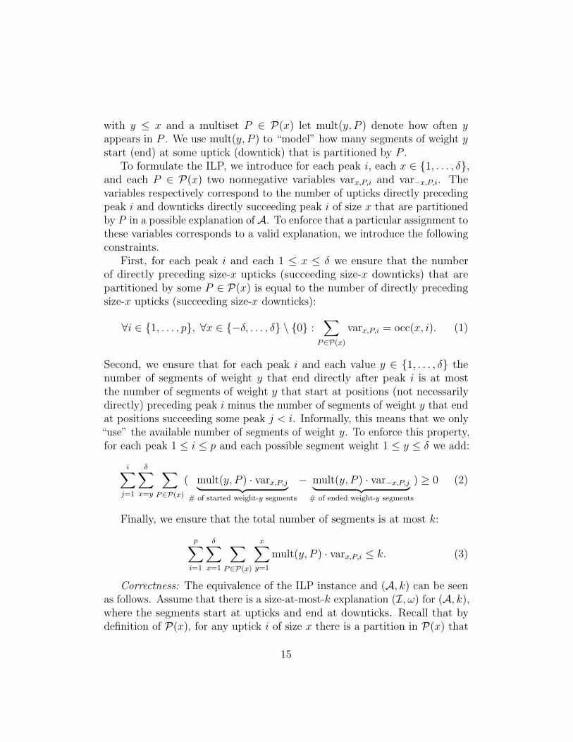
In the ILP formulation for VPE, we describe a solution by “fixing” foreach position i a multiset Xi of positive integers which partitions the uptick(downtick) at i. The crucial observation for our ILP is that if a set ofconsecutive upticks contains more than one uptick of size x, then it is sufficientto fix how many of these upticks were partitioned in which way. In other words,one does not need to know the partition for each position; instead one candistribute freely the partitions of x onto the upticks of size x. This also holdsfor consecutive downticks. Since each peak is preceded by consecutive upticksand succeeded by consecutive downticks, and since we introduce variables inthe ILP formulation to “model” how many upticks (downticks) exist betweentwo consecutive peaks, the number of variables in the formulation is upper-bounded by a function of p and δ. We now give the details of the formulation.Herein, we assume that the peaks are ordered from left to right; we refer tothe i-th peak in this order as peak i.
For an integer x ∈ {1, . . . , δ}, let occ(x, i) denote the number of upticks ofsize x that directly precede peak i, that is, the number of upticks succeedingpeak i−1 and preceding peak i. Similarly, let occ(−x, i) denote the number ofdownticks of size x that directly succeed i. For two positive integers y and x
14
with y ≤ x and a multiset P ∈ P(x) let mult(y, P ) denote how often yappears in P . We use mult(y, P ) to “model” how many segments of weight ystart (end) at some uptick (downtick) that is partitioned by P .
To formulate the ILP, we introduce for each peak i, each x ∈ {1, . . . , δ},and each P ∈ P(x) two nonnegative variables varx,P,i and var−x,P,i. Thevariables respectively correspond to the number of upticks directly precedingpeak i and downticks directly succeeding peak i of size x that are partitionedby P in a possible explanation of A. To enforce that a particular assignment tothese variables corresponds to a valid explanation, we introduce the followingconstraints.
First, for each peak i and each 1 ≤ x ≤ δ we ensure that the numberof directly preceding size-x upticks (succeeding size-x downticks) that arepartitioned by some P ∈ P(x) is equal to the number of directly precedingsize-x upticks (succeeding size-x downticks):
Second, we ensure that for each peak i and each value y ∈ {1, . . . , δ} thenumber of segments of weight y that end directly after peak i is at mostthe number of segments of weight y that start at positions (not necessarilydirectly) preceding peak i minus the number of segments of weight y that endat positions succeeding some peak j < i. Informally, this means that we only“use” the available number of segments of weight y. To enforce this property,for each peak 1 ≤ i ≤ p and each possible segment weight 1 ≤ y ≤ δ we add:
i∑j=1
δ∑x=y
∑P∈P(x)
( mult(y, P ) · varx,P,j︸ ︷︷ ︸# of started weight-y segments
− mult(y, P ) · var−x,P,j︸ ︷︷ ︸# of ended weight-y segments
) ≥ 0 (2)
Finally, we ensure that the total number of segments is at most k:
p∑i=1
δ∑x=1
∑P∈P(x)
x∑y=1
mult(y, P ) · varx,P,i ≤ k. (3)
Correctness: The equivalence of the ILP instance and (A, k) can be seenas follows. Assume that there is a size-at-most-k explanation (I, ω) for (A, k),where the segments start at upticks and end at downticks. Recall that bydefinition of P(x), for any uptick i of size x there is a partition in P(x) that
15
corresponds to the weights of the segments starting in i. For each peak i, forany value 1 ≤ x ≤ δ and each P ∈ P(x), count how many upticks of size xthat directly precede peak i are explained by segments in I (segments thatstart in this uptick) whose weights correspond to P(x) and set varx,P,i to thisvalue. Symmetrically, do the same for the downticks succeeding peak i andset var−x,P,i accordingly. It is straightforward to verify that Constraint set (1)and Constraint set (2) and constraint (3) hold.
Conversely, assume that there is an assignment to the variables such thatConstraint sets (1) and (2) and Constraint (3) are fulfilled. We form anexplanation (I, ω) as follows: For any peak i and any value 1 ≤ x ≤ δ withocc(x, i) > 0 let Pi,x be the multiset of elements from P(x) that containseach P ∈ P(x) exactly varx,P,i times. By Constraint set (1), |Pi,x| = occ(x, i).For an arbitrary ordering of Pi,x and the upticks of size x directly precedingpeak i, add to I for the jth element Pj of Pi,x exactly |Pj| segments withweight corresponding to Pj and let them start at the jth uptick with size xthat directly precedes peak i. By Constraint (3) we added at most k segments.It remains to specify the end of the segments. Symmetrically to the upticks,for each downtick directly succeeding peak i of size x let Pi,x be the multiset ofelements from P(x) containing each P ∈ P(x) exactly var−x,P,i times. For thejth element Pj of Pi,x and the jth downtick directly succeeding peak i (againboth with respect to any ordering) and for each α ∈ Pj pick any weight-αsegment from I (so far without end) and let it at the jth downtick. Observethat the existence of this segment is ensured by Constraint set (2). Finally,it remains to argue that the end of each segment in I is determined. Thisfollows from the fact that Constraint set (1) and Constraint set (2) togetherimply for each 1 ≤ y ≤ δ that
p∑i=1
δ∑x=y
∑P∈P(x)
(mult(y, P ) · varx,P,i−mult(y, P ) · var−x,P,i) = 0,
and thus the total number of opened weight-y segments is equal to the numberof ended weight-y segments.
Running time: The number of variables in the constructed ILP instance is
p ·∑
x∈{−δ,...,δ}\{0}
|P(|x|)| = 2pδ∑
x=1
|P(x)| ≤ 2δp · |P(δ)| ≤ 2δp ·eπ√
23δ =: f(δ, p),
where the last inequality is due to de Azevedo Pribitkin [2]. Then, due toa deep result in combinatorial optimization, the feasibility of the ILP can
16
be decided in O(f(δ, p)2.5f(δ,p)+o(f(δ,p)) · |L|) time, where |L| is the size of theinstance [17, 21, 25]. Moreover, as we have O(δp) constraints, we also have
|L| = O(δ2p2 · eπ√
23δ).
Observe that Theorem 3.1 implies that VE is fixed-parameter tractablewith respect to the maximum difference δ: By Corollary 2.2(ii) & Corol-lary 2.4(i), in linear time one can transform input instances of VE intoequivalent single-peaked instances of VPE without increasing the maximumdifference δ.
Corollary 3.2. Vector Explanation parameterized by the maximumdifference δ is fixed-parameter tractable.
It remains open whether VPE is fixed-parameter tractable with respectto δ. Note that the argumentation for VE (Corollary 3.2) cannot be trans-ferred, since there may be more than one peak in an instance. However,thefollowing theorem shows that VPE is in XP for the parameter maximumdifference δ.
Theorem 3.3. Vector Positive Explanation is solvable in O(nδ ·eπ√
2δ/3) time.
Proof. We describe a dynamic programming algorithm that finds a regularminimum-size explanation. Every explanation for a size-n vector A can beinterpreted as an extension of an explanation for the same vector without thelast entry, where some segments that originally only covered position n− 1may be stretched to also cover position n and some new length-one segmentmay start at position n.
Our algorithm uses the above relation between explanations for the vec-tor A[1, . . . , n] and explanations for the vector A[1, . . . , n− 1]. Due to Theo-rem 2.1, it only considers regular explanations, implying that each segmentstarts at an uptick and ends at a downtick. Since all upticks and downtickshave size at most δ, the algorithm furthermore only considers solutions inwhich all segments have weight at most δ.
We fill a table T which has entries of type T (i, d1, . . . , dj, . . . , dδ) where0 ≤ i ≤ n and 0 ≤ dj ≤ k with 1 ≤ j ≤ δ. An entry T (i, d1, . . . , dj, . . . , dδ)contains the minimum number of segments explaining vector A[1, . . . , i] suchthat dj segments of weight j cover position i. If no such explanation exists,
17
then the entry is set to ∞. By definition of the table entries, there is asolution for VPE if and only if
min(d1,...,dδ)∈{0,...,k}δ
T (n, d1, . . . , dδ) ≤ k.
In the following, we show how to fill the table. As initialization, setT (0, d1, . . . , dδ)←∞ if there is some dj > 0 and set T (0, 0, . . . , 0)← 0.
For increasing i ≤ n, compute the table for each (d1, . . . , dδ) ∈ {0, . . . , k}δas follows. If A[i] =
∑δj=1 dj · j and A[i] > A[i− 1], then set
T (i, d1, . . . , dδ)← mind′1≤d1,...,d′δ≤dδ
(T (i− 1, d′1, . . . , d
′δ) +
δ∑j=1
(dj − d′j)
). (4)
If A[i] =∑δ
j=1 dj · j and A[i] < A[i− 1], then set
T (i, d1, . . . , dδ)← mind′1≥d1,...,d′δ≥dδ
T (i− 1, d′1, . . . , d′δ). (5)
Otherwise, set
T (i, d1, . . . , dδ)←∞. (6)
The correctness of the initialization follows directly from the table defini-tion. For the remaining computation we can thus assume that there is some isuch that all entries T (i′, d1, . . . , dδ) with (d1, . . . , dδ) ∈ {0, . . . , k}δ and i′ < iwere computed correctly.
As discussed above, we interpret an explanation of A[1, . . . , i] as extensionof an explanation for A[1, . . . , i−1]. There are exactly two groups of segmentscovering position i: those also covering position i − 1 and those startingat position i. Let the set of segments covering position i be describedby (d1, . . . , dδ) such that A[i] =
∑δj=1 dj · j and A[i] > A[i − 1]. Due to
Theorem 2.1, no segment ends at position i, but since A[i] > A[i − 1] atleast one new segment has to start at position i. By setting (d′1, . . . , d
′δ)
such that d′j ≤ dj, 1 ≤ j ≤ δ, one considers all possible extensions forexplanations of A[i − 1] such that no segment ends at position i. Clearly,∑δ
j=1(dj − d′j) further segments have to start at position i to explain A[i].Hence, Assignment (4) is correct.
Now, describe the set of segments covering position i by (d1, . . . , dδ) suchthat A[i] =
∑δj=1 dj · j and A[i] < A[i− 1]. By Theorem 2.1 no new segment
18
starts at position i. The algorithm considers all possible explanations wheresome segments end at position i and the other segments survive to explain A[i].Thus, Assignment (5) is correct.
For a given (d1, . . . , dδ) ∈ {0, . . . , k}δ, to find an explanation for A[1, . . . , i]such that A[i] 6=
∑δj=1 dj · j is impossible because such an explanation does
not explain position i. Thus Assignment (6) is correct.The size of the table is upper-bounded by nδ since we only have to consider
table entries T [i, d1, . . . , dδ] with A[i] =∑δ
j=1(dj · j). The trivial upper bound
of O(nδ) for computing each table entry already leads to a running timeof O(n2δ). However, the number of entries that have to be considered issmaller. For Assignment (4), one only has to consider those entries of Table Tthat do not have value ∞. Hence,
∑δj=1 |dj − d′j| ≤ |A[i] − A[i − 1]| ≤
δ. This implies that for each table entry the number of previous entriesthat have to be considered in the minimization is upper-bounded by thenumber of different multisets that sum up to δ and thus is upper-bounded
by O(eπ√
23δ) [2]. A similar argument applies for Assignment (5). The overall
running time follows.
VPE is known to be fixed-parameter tractable when parameterized bythe maximum value γ [6]. We complement this result by showing a lowerbound on the kernel size, and thus demonstrate limitations on the power ofpolynomial-time preprocessing.
Theorem 3.4. Unless NP ⊆ coNP/poly, there is no polynomial kernel forVector Positive Explanation parameterized by the maximum value γ.
Proof. We provide an AND-cross-composition [7, 11] from the 3-Partitionproblem [18, SP15]. This is a polynomial-time algorithm that gets as input aset of 3-Partition-instances and computes an instance (A, k) of VPE suchthat the maximum value γ occurring in (A, k) is polynomially bounded inthe maximum of sizes of the input 3-Partition instances and (A, k) is ayes-instance if and only if all given 3-Partition instances are yes-instances.
3-PartitionInput: A multiset S = {a1, . . . , a3m} of positive integers and aninteger bound B with m ·B =
∑3mi=1 ai and B/4 < ai < B/2 for every
i ∈ {1, . . . , 3m}.Question: Is there a partition of S into m subsets P1, . . . , Pm with|Pj| = 3 and
∑ai∈Pj ai = B for every j ∈ {1, . . . ,m}?
19
3-Partition is NP-complete even if B (and thus all ai’s) is bounded by apolynomial in m [18]. We show that this variant of 3-Partition AND-cross-composes to VPE parameterized by the maximum value γ. Then, resultsof Bodlaender et al. [7] and Drucker [11] imply that VPE does not have apolynomial kernel with respect to parameter γ, unless NP ⊆ coNP/poly.
First, let (S,B) be a single instance of 3-Partition. We show that itreduces to an instance (A′, 3m) of VPE. This reduction is similar to a previousNP-hardness reduction for VPE due to Bansal et al. [4]. We define A′ aslength-(4m− 1) vector:(
a1, a1 + a2, . . . ,
j∑i=1
ai, . . . ,3m∑i=1
ai = mB, (m− 1)B, (m− 2)B, . . . , B
).
If a partition P1, . . . , Pm of S forms a solution, then the set of segments{[i, 3m+ j] | ai ∈ Pj} each with weight w([i, 3m+ j]) = ai is an explanationfor the vector A′. Conversely, let (I, ω) be a regular explanation for (A′, 3m).Since every segment starts at an uptick and ends at a downtick, I contains 3msegments and the segment starting at position i has weight ai. Since B/4 <ai < B/2 for each integer ai ∈ S, exactly three segments end at a downtickwhose size is exactly B. Thus, grouping the segments according to theposition they end at, we get the desired partition of S, solving the instanceof 3-Partition.
Now let (S1, B1), . . . , (St, Bt) be instances of 3-Partition such that Sr ={ar1, . . . , ar3mr} and Br ≤ mr
c for every r ∈ {1, . . . , t} and some constant c.We build an instance (A, k) of VPE by first using the above reduction foreach (Sr, Br) separately to produce a vector A′r, and then concatenating thevectors A′r one after another, leaving a single position of value 0 in between.The total length of the vector A is 4(
∑tr=1mr)− 1 and we set k = 3
∑tr=1mr.
Due to the argumentation for the single instance case, on the one hand,if each of the instances is a yes-instance, then there is an explanation us-ing 3mr segments per instance (Sr, Br), that is 3
∑tr=1mr segments in total.
Conversely, we need at least 3mr segments to explain A′r and there is anexplanation with 3mr segments if and only if (Sr, Br) is a yes-instance. Sinceall segments are positive and the subvectors A′r are separated by an entrywith value zero, no segment can span over two subvectors. In other words,no segment can be used to explain more than one of the A′r’s. Therefore,an explanation for A with 3
∑tr=1mr segments implies that (Sr, Br) is a
yes-instance for every r ∈ {1, . . . , t}.
20
Finally, observe that the maximum value γ in the vector A is equalto maxtr=1mrBr ≤ maxtr=1mr
c+1 and, thus, it is polynomially boundedin maxtr=1 |Sr|. Hence, 3-Partition AND-cross-composes to VPE parame-terized by the maximum value γ, and there is no polynomial kernel for thisproblem unless NP ⊆ coNP/poly.
4. Parameterizations of the Size and the Structure of Solutions
We now provide fixed-parameter tractability and (parameterized) hardnessresults for further natural parameters. Specifically, we consider the number kof segments in the solution, so-called “above-guarantee” and “below-guarantee”parameterizations (which are smaller than k), the maximum segment length ξ,and the maximum number φ of segments covering a position.
For the parameter k we develop a search tree algorithm for VPE and VEwhere the depth and the branching degree of the search tree are boundedby the solution size k. This is achieved by combining Reduction Rule 1.1,Corollary 2.2, and Corollary 2.4. The first part of Theorem 4.1 follows directlyfrom exhaustively applying Reduction Rule 1.1.
Theorem 4.1. Any instance of Vector Positive Explanation or Vec-tor Explanation can be reduced in O(n) time to an equivalent one with atmost (2k − 1) entries. Furthermore, Vector Positive Explanation andVector Explanation can be solved in O(k! · k + n) time.
Proof. We start with the algorithm for VPE which works as follows. Afterexhaustive application of Reduction Rule 1.1 branch over all possible segmentscovering the last entry. Due to Corollary 2.2(i), it suffices to search for exactlyone segment starting at one of the upticks and ending at the last entry. Foreach branch assign the value A[n] as weight to the segment and solve theinstance consisting of the remaining entries recursively. To this end, decreaseeach of the entries covered by the segment by A[n], and decrease k by one. Ifsome entry becomes negative or if k < 0, then discard the branch.
The exhaustive application of Reduction Rule 1.1 can be performed in O(n)time, afterwards n ≤ 2k − 1 (this also implies the first part of the theorem).The search tree produced by the branching algorithm has depth at most k. Inthe i-th level of the search tree, one branches over at most k + 1− i upticks.The steps performed in each search tree node take O(k) time since n ≤ 2k−1.The overall running time thus is O(k! · k + n).
21
For VE we first apply Corollary 2.4(i) to transform our instance into asingle-peaked instance (this is necessary to avoid negative entries). The restworks analogously to VPE.
The first part of Theorem 4.1 implies that for a reduced instance everyexplanation needs at least bn/2c+1 segments. Hence, it is interesting to studyparameters that measure how far we have to exceed this lower bound for thesolution size: such above-guarantee parameters can be significantly smallerthan k. For this reason, we study a parameter that measures k− (bn/2c+ 1).For ease of presentation, we define this parameter as κ := 2k − n. Theconcepts of “clean” and “messy” positions, which are defined as follows, arecrucial for the design of our algorithms.
Definition 4.1. Let (A, k) be an instance of Vector Explanation orVector Positive Explanation and let I be an explanation for A. Asegment I = [i, j] ∈ I is clean if all other segments start and end at positionsdifferent from i and j. A position i is clean with respect to I if it is the startor endpoint of a clean segment in I. A position or segment that is not cleanis called messy.
Remark: Note that a segment is messy if and only if it is in one of the messyoverlapping configurations shown in Figure 2.1.
Messy positions and segments have the following useful relation to theparameter κ: if κ is small, then there are only few messy positions andsegments.
Lemma 4.2. Let (A, k) be a yes-instance of Vector Positive Expla-nation that is reduced with respect to Reduction Rule 1.1. Then, everyexplanation of (A, k) of size at most k has at most 2κ messy segments and atmost 3κ messy positions.
Proof. Let x denote the number of messy segments in some arbitrary expla-nation for (A, k). Since (A, k) is reduced with respect to Reduction Rule 1.1,every position of A is the starting point or endpoint of some segment. Inparticular, every messy segment shares at least one endpoint with anothermessy segment. Hence, there are at most 3x/2 messy positions in the explana-tion. Furthermore, since there are at most k − x clean segments there are atmost 2(k−x) clean positions. Thus, n ≤ 2(k−x)+3x/2 which implies x ≤ 2κ,and the number of messy positions is at most (3x/2) ≤ 3κ.
22
H
h `
I
i j
H ′h j
I ′i `
H
h `
I
i j
H ′h j
I ′i `
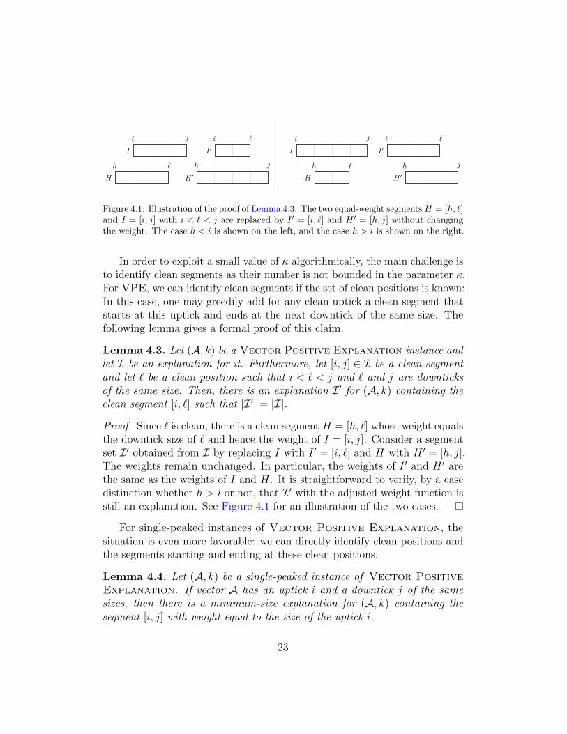
Figure 4.1: Illustration of the proof of Lemma 4.3. The two equal-weight segments H = [h, `]and I = [i, j] with i < ` < j are replaced by I ′ = [i, `] and H ′ = [h, j] without changingthe weight. The case h < i is shown on the left, and the case h > i is shown on the right.
In order to exploit a small value of κ algorithmically, the main challenge isto identify clean segments as their number is not bounded in the parameter κ.For VPE, we can identify clean segments if the set of clean positions is known:In this case, one may greedily add for any clean uptick a clean segment thatstarts at this uptick and ends at the next downtick of the same size. Thefollowing lemma gives a formal proof of this claim.
Lemma 4.3. Let (A, k) be a Vector Positive Explanation instance andlet I be an explanation for it. Furthermore, let [i, j] ∈ I be a clean segmentand let ` be a clean position such that i < ` < j and ` and j are downticksof the same size. Then, there is an explanation I ′ for (A, k) containing theclean segment [i, `] such that |I ′| = |I|.
Proof. Since ` is clean, there is a clean segment H = [h, `] whose weight equalsthe downtick size of ` and hence the weight of I = [i, j]. Consider a segmentset I ′ obtained from I by replacing I with I ′ = [i, `] and H with H ′ = [h, j].The weights remain unchanged. In particular, the weights of I ′ and H ′ arethe same as the weights of I and H. It is straightforward to verify, by a casedistinction whether h > i or not, that I ′ with the adjusted weight function isstill an explanation. See Figure 4.1 for an illustration of the two cases.
For single-peaked instances of Vector Positive Explanation, thesituation is even more favorable: we can directly identify clean positions andthe segments starting and ending at these clean positions.
Lemma 4.4. Let (A, k) be a single-peaked instance of Vector PositiveExplanation. If vector A has an uptick i and a downtick j of the samesizes, then there is a minimum-size explanation for (A, k) containing thesegment [i, j] with weight equal to the size of the uptick i.
23
Proof. Let (A, k) be a single-peaked VPE instance and let T be the tickvector of A. By Corollary 2.2(ii) (A, k) is an equivalent VE instance andthus by Theorem 2.3 we may assume that j = i+ 1. Furthermore, let (I, ω)be a regular minimum-size explanation of (A, k). Let Is be all segments in Istarting in i and let Ie be all segments in I ending in i+ 1 and, additionally,do not start in i. Hence Is ∩ Ie = ∅.
Let T ′ be a copy of T and “subtract” the segments in I \(Is∪Ie): For eachsegment [`, r] ∈ I \ (Is ∪ Ie) of weight a decrease T ′[`] by a and increase T ′[r]by a. Additionally, subtract [i, i + 1] with weight T [i], meaning that weset T ′[i] and T ′[i + 1] from ±T [i] to zero. Observe that if there is a size-(|Is| + |Ie| − 1) explanation for the input vector corresponding to T ′, thencombining this explanation with the segments from I \ (Is ∪ Ie) and thesegment [i, i+ 1] of weight T [i] gives a minimum-size explanation for (A, k).Thus, it remains to show that there is a size-(|Is| + |Ie| − 1) explanationfor the input vector corresponding to T ′. Since we subtracted all segmentsin I \(Is∪Ie), all positions in T ′ that have nonzero entries are the start or endof a segment in Is ∪ Ie. Moreover, since we additionally subtracted [i, i+ 1]with weight T [i], there are at most |Ie| upticks and at most |Is| downticksin T ′. Hence, the corresponding input vector of T ′ has, after an application ofReduction Rule 1.1, at most |Ie|+ |Is| − 1 entries. Therefore, it has a trivialexplanation of size at most |Ie|+ |Is| − 1.
We now have all ingredients to provide our two tractability results withrespect to the parameter κ. More precisely, we show membership in XP forVPE and fixed-parameter tractability for VE and single-peaked VPE. Themain approach of the algorithms is as follows: For VPE, we guess all messypositions, then we greedily identify the clean segments (using Lemma 4.3),and then we solve the remaining instance (which now has size bounded in κ).For single-peaked VPE and VE, we can directly reduce the instance to onethat has only messy positions (using Lemma 4.4).
Theorem 4.5. (i) Vector Positive Explanation can be solved inO((2k)3κ · (2κ)! · κ · k + k log k + n) time.
(ii) Any single-peaked instance of Vector Positive Explanation andany instance of Vector Explanation can be reduced in O(n +k log k) time to an equivalent instance with at most 3κ entries. More-over, Vector Explanation and single-peaked Vector PositiveExplanation are solvable in O((2κ)! · κ+ k log k + n) time.
24
Proof of Theorem 4.5(i). We prove that VPE can be solved in O((2k)3κ ·(2κ)! · κ · k + k log k + n) time. Let (A, k) be an instance of VPE and let Tbe the tick vector corresponding to A. We may assume via a preprocessingstep running in O(n) time that Reduction Rule 1.1 has been exhaustivelyapplied and thus the number of positions is at most 2k.
The algorithm works as follows. Let U (D) be the set of all upticks(downticks) in T . Sort the values in U and D in ascending order accordingto their absolute sizes and use their position in T as a tie-breaker (smallerpositions come first). This can be done in O(k log k) time. Next, branchinto the at most (2k)3κ possibilities for choosing all of the at most 3κ messypositions (Lemma 4.2). If the guess was correct, then for each clean uptickthere is a clean downtick of equal size.
By Lemma 4.3 there is a minimum-size explanation that contains a segmentstarting in any clean uptick position i and ending at the first clean downtickposition j > i with the same size. We next find and remove these segments:Initialize k by the value of k and also T ′ by T . Iterate over all clean upticksin the order of U and find for each of them the first clean downtick in Dwhich starts to its right. Delete the up- and downtick from T ′ and decreaseparameter k by one. Clearly, by using two pointers, one for U and one for D,iterating over U and finding the downtick in D can be done in O(k) timeas by the order of U and D one has to move the pointers only to the right.Moreover, if at some point of the iteration we do not find any “matching”downtick or at the end there remain some clean downticks in D, then weabort this branch as the guess of clean positions was incorrect. Let A′ bethe input vector corresponding to the final T ′. Note that since all positionsin A′ are messy, by Lemma 4.2 it follows that |A′| ≤ 2κ and k ≤ 3κ. Hence,Theorem 4.1 solves the remaining instance (A′, k) in O((2κ)! · κ) time. Theoverall running time is O((2k)3κ · (2κ)! · κ · k + k log k + n).
Proof of Theorem 4.5(ii): Due to Corollary 2.4(i), we can assume thatthe given instance of VE is single-peaked. Also, because of Corollary 2.2(ii),we only need to investigate whether the given single-peaked instance is ayes-instance for VPE. We first apply Reduction Rule 1.1 exhaustively. Afterthat, if there is an uptick and a downtick of the same size, then by Lemma 4.4there is an optimal solution containing a segment starting at the uptick andending at the downtick of weight equal to the size of the uptick. Hence,by applying a similar procedure as in the proof of Theorem 4.5(i) (sort up-and downticks by their size) one finds and eliminates all these segments inO(k log k) time. Note that by removing such a segment from the input vector
25
the length of the vector is reduced by two, while k is reduced by one, so κstays the same.
In the remaining instance all positions are messy and thus by Lemma 4.2there are at most 3κ messy positions and 2κ messy segments explainingthem. Thus, one ends up with a problem kernel having at most 3κ positions.By Theorem 4.1, this kernel can be solved in O((2κ)! · 2κ+ 3κ) time.
Theorem 4.5(ii) implies that single-peaked VPE and VE are fixed-parameter tractable with respect to κ. For VPE, we obtained a polynomial-time algorithm for every fixed value of κ but not a fixed-parameter algorithmfor κ. As we show in the following, such an algorithm is unlikely.
Theorem 4.6. Vector Positive Explanation is W[1]-hard with respectto κ.
Proof. We present a parameterized reduction from the Subset Sum problem.
Subset Sum [18, SP13]Input: A multiset X = {x1, . . . , x`} of positive integers and twopositive integers y and Φ.Question: Is there a size-Φ subset X ′ of X such that
∑xi∈X′ xi = y?
Subset Sum is W[1]-hard with respect to the solution size Φ [13]. In thefollowing, we use t :=
∑1≤i≤` xi to denote the total sum of the integers in X.
Note that by modifying the xi’s we can assume that for every size-(Φ − 1)subset X ′ the sum
∑xi∈X′ xi is less than y: adding t to each input integer,
and Φ · t to y results in an instance for which this holds. Next, we describethe parameterized reduction.
The input vector A has length 2`+ 1. For i ≤ `, we set A[i] :=∑i
j=1 xj.Let A[`+ 1] = t−y. For i ≥ `+ 2, we set A[i] = A[2`+ 2− i]. The number ofallowed segments is set to `+Φ. Consequently, κ = 2(`+Φ)−(2`+1) = 2Φ−1.
We complete the proof by showing that for this construction the followingequivalence holds.
(X, y,Φ) is a yes-instance of Subset Sum ⇔ (A, ` + Φ) is ayes-instance of VPE.
“⇒”: Let X ′ be a size-Φ subset of X whose values sum up to y. Then,consider the following set I of segments.
For each xi /∈ X ′, add the segment Ji = [i, 2` + 3 − i]. There are` − Φ such segments. For each xi ∈ X ′, add two segments Ii = [i, ` + 1]
26
and I ′i = [` + 2, 2` + 3 − i]. For each of these two types of segments thereare Φ of them. Hence, |I| = ` + Φ. For each 1 ≤ i ≤ ` set the weights ofthe segments Ji, Ii and I ′i to xi. Now, I explains A: First, for each i ≤ `,A[i] =
∑j≤i xj is explained by {Jj | j ≤ i∧ xj /∈ X ′} ∪ {Ij | j ≤ i∧ xj ∈ X ′}.
Second, A[`+ 1] = t− y is explained by exactly the segments Jj with xj /∈ X ′.Finally, for i > ` + 1, A[i] = A[2` + 2 − i] =
∑j≤2`+2−i xj is explained by
{Jj | j ≤ 2`+ 2− i ∧ xj /∈ X ′} ∪ {I ′j | j ≤ 2`+ 2− i ∧ xj ∈ X ′}.“⇐”: Let I be a set of `+ Φ segments that explain A. By Theorem 2.1
we can assume that I is regular. First, note that for each position i ≤ `,there is at least one segment that starts at i. Also, each of these segmentshas a weight of at most the maximum value in X. Since for any X ′ with|X ′| < Φ it holds that
∑xi∈X′ xi < y and the size of downtick `+ 1 is y, at
least Φ segments end at `+ 1. Similarly, for each i ≥ `+ 3 there is at leastone segment that ends at position i, and each of these segments has a weightof at most xj for some xj ∈ X. Further, since the size of uptick `+ 2 is y, atleast Φ segments start at `+ 2. This implies that there are exactly ` segmentsstarting in the first ` positions and exactly Φ segments ending at position `+1.Therefore, for each i ≤ ` there is exactly one segment starting at i which hasweight xi. Since Φ of these segments end at position `+ 1, they correspondto a size-Φ set X ′ ⊆ X. Finally, since A[`] = t and A[` + 1] = t − y thesum
∑xi∈X′ xi of the integers in this set is exactly y.
Parameter κ used in Theorems 4.5 and 4.6 measures to what extentthe solution exceeds the lower bound bn/2c + 1. Another bound on thesolution size is n: If k = n, then any instance of VPE or VE is a trivial yes-instance. Hence, it is interesting to consider the parameter n−k. Furthermore,it is natural to consider explanations with restricted segment length ξ orthe maximum number φ of segments overlapping at some position. Thefollowing theorem shows that VPE and VE are already NP-complete even ifk = n− 1, ξ ≥ 3, and φ = 2. To this end, we reduce from the NP-completePartition problem [18, SP12]. In terms of parameterized complexity thisimplies that, unless P=NP, VPE is not fixed-parameter tractable with respectto the “maximum segment length ξ”, the “maximum number φ of segmentsoverlapping at some position”, and the “below guarantee parameter” n− k.
Theorem 4.7. Vector Positive Explanation and Vector Explana-tion are weakly NP-complete even if k = n− 1 and every yes-instance has anexplanation of at most k segments where each position is covered by at mosttwo segments and each segment has length at most three.
27
Proof. We reduce from the weakly NP-complete Partition problem.
Partition [18, SP12]Input: A multiset of positive integers S = {a1, . . . , at}.Question: Is there a subset S ′ ⊆ S such that
∑ai∈S′ ai =∑
ai∈S\S′ ai?
Given an instance S = {a1, . . . , at} of Partition, we create an inputinstance (A, k), where A is a vector of length 3t + 1 and k = 3t. Morespecifically, AT is the vector
Obviously, the reduction runs in polynomial time. It remains to show that
S = {a1, . . . , at} is a yes-instance of Partition ⇔ (A, k = 3t) isa yes-instance of VPE and VE.
“⇒”: Let S ′ ⊆ S be a solution for the Partition instance, meaningthat
∑ai∈S′ ai =
∑ai∈S\S′ ai. Further, let S ′j := S ′ ∩ {a1, . . . , aj}, Sj :=
{a1, . . . , aj} \ S ′, and S ′0 = S0 := ∅. We construct the set I of segmentsconsisting of six subsets and their weights as follows (we use the notation[`, r; a] for a weight-a segment that starts at `, ends at r and does notinclude r):
28
I1 = {[3j − 2, 3j + 1; j + (t+ 1) ·∑
ai∈S′j−1
ai] | aj /∈ S ′},
I2 = {[3j − 1, 3j; j + (t+ 1) ·∑
ai∈Sj−1
ai] | aj /∈ S ′},
I3 = {[3j, 3j + 2; j + (t+ 1) ·∑ai∈Sj
ai] | aj /∈ S ′},
I4 = {[3j − 1, 3j + 2; j + (t+ 1) ·∑
ai∈Sj−1
ai] | aj ∈ S ′},
I5 = {[3j − 2, 3j; j + (t+ 1) ·∑
ai∈S′j−1
ai] | aj ∈ S ′},
I6 = {[3j, 3j + 1; j + (t+ 1) ·∑ai∈S′j
ai] | aj ∈ S ′}.
As there are exactly three segments for each aj, there are 3t segments intotal. Note that if aj /∈ S ′, then S ′j−1 = S ′j . Otherwise aj /∈ S ′ and Sj−1 = Sj .
Now, we show that I with weight function ω explains vector A. Let j ∈{1, . . . , t}. At position 3j − 2 = 3(j − 1) + 1 we have A[3j − 2] = 2j −1 + (t+ 1)
∑j−1i=1 ai. If aj /∈ S ′, then segment [3j − 2, 3j + 1] from I1 covers
3j − 2 and if aj ∈ S ′, then segment [3j − 2, 3j] from I5 covers 3j − 2. Bothsegments have weight j + (t+ 1)
∑ai∈S′j−1
ai. Additionally, if aj−1 /∈ S ′, then
segment [3(j − 1), 3(j − 1) + 2] from I3 also covers 3j − 2 and if aj−1 ∈ S ′,then segment [3(j − 1)− 1, 3(j − 1) + 2] from I4 also covers 3j − 2. In bothcases the weight of the segment is (j − 1) + (t+ 1)
∑ai∈Sj−1
ai. In the former
case this holds by definition. In the latter case, since aj−1 ∈ S ′, it holds thataj−1 /∈ S ′ and, thus, S ′j−2 = S ′j−1. Summarizing, in each case the weights ofthe two segments covering position 3j − 2 sum up toj + (t+ 1) ·
∑ai∈S′j−1
ai
+
(j − 1) + (t+ 1) ·∑
ai∈Sj−1
ai
= 2j − 1 + (t+ 1) ·
j−1∑i=1
ai
=A[3j − 2].
29
In the same way, at position 3j−1, we have A[3j−2] = 2j+(t+1)∑j−1
i=1 ai.If aj /∈ S ′, then only segments [3j − 2, 3j + 1] from I1 and [3j − 1, 3j] from I2cover and explain this position, sincej + (t+ 1) ·
∑ai∈S′j−1
ai
+
j + (t+ 1) ·∑
ai∈Sj−1
ai
= 2j + (t+ 1) ·
j−1∑i=1
ai
=A[3j − 1].
Otherwise, only segments [3j − 1, 3j + 2] from I4 and [3j − 2, 3j] from I5cover and explain this position, sincej + (t+ 1) ·
∑ai∈Sj−1
ai
+
j + (t+ 1) ·∑
ai∈S′j−1
ai
= 2j + (t+ 1) ·
j−1∑i=1
ai
=A[3j − 1].
Also, at position 3j, we have A[3j] = 2j +∑j
i=1 ai. If aj /∈ S ′, then onlysegments [3j − 2, 3j + 1] from I1 and [3j, 3j + 2] from I3 cover and explainthis position since the sum of their weights equalsj + (t+ 1) ·
∑ai∈S′j
ai
+
j + (t+ 1) ·∑ai∈Sj
ai
= 2j + (t+ 1) ·
j∑i=1
ai
=A[3j].
This also holds for the case that aj ∈ S ′. Finally, we have only one segment
30
covering the position 3t+ 1 with weight
t+ (t+ 1)∑ai∈St
ai = t+ (t+ 1) ·∑
ai∈S\S′ai
= t+1
2(t+ 1) ·
t∑i=1
ai
= A[3t+ 1].
“⇐”: Let I with weights ω be a regular explanation for vector A withat most k segments. As all upticks precede all downticks, all segments in Iare positive. More precisely, as there are exactly k = 3t upticks, exactly onepositive segment starts at every uptick and ends either at position 3t+ 1 or3t+ 2.
We denote the segment of I starting at position 3i by Ii. Obviously,ω(Ii) = (t+ 1) · ai. Furthermore, there are 2t segments of weight one. Nowset S ′ := {ai | Ii ends at position 3t + 2}. We show that S ′ is a solution ofthe Partition instance S: Let x ∈ {0, . . . , 2t} be the number of segments ofweight 1 that cover position 3t+1. We have x+(t+1)
∑ai∈S′ ai = A[3t+1] =
t+ 12(t+ 1) ·
∑ti=1 ai. As |t− x| ≤ t, we have
∑ai∈S′ ai = 1
2
∑ti=1 ai. Hence,
S ′ is a solution for the Partition instance S.As we can see from the reduction, every yes-instance of Partition is
reduced to a yes-instance that can be explained by segments with ξ = 3and φ = 2 and every no-instance is reduced to an instance that cannot beexplained by segments of any size. The statement of Theorem 4.7 follows.
Next, we show that, in contrast to the NP-completeness for ξ ≥ 3 (Theo-rem 4.7), VPE and VE are polynomial-time solvable for ξ ≤ 2.
Theorem 4.8. Vector Explanation and Vector Positive Explana-tion can be solved in O(n2) time for maximum segment length ξ = 2.
Proof. We devise a dynamic programming algorithm for VPE. Afterwards,we show how to extend our algorithm to VE.
Let (A, k) be an input instance, whereA is a vector of length n. Since ξ = 2we may assume that the last position is only covered by either one length-twosegment or one length-one segment, but not both: otherwise, there are twolength-two segments covering the last position which can be transformed intoa solution with two length-one segments. Due to this, if we have an optimal
31
solution for a vector of length x, then we can find an optimal solution for avector of length x+ 1 which contains either an additional length-one segmentor a length-two segment covering the last position.
Based on this idea, we use dynamic programming with a table D indexedby 1, . . . , n: For each j ≤ n, we store in D(j) the minimum number ofsegments needed to explain the subvector A[1, . . . , j]. Let D(0) = 0 forsimplicity. For j = 1, we set D(1) = 1 which is obviously correct. Nowassume that for an index j ≤ n, D(i) was already computed for each i < jand we now compute D(j). We begin with i := j and aji := A[j]. We set
aji−1 := A[i− 1]− aji and i := i− 1
as long asaji > 0 and i > 1. (*)
The idea behind this computation is that we can assume that each chainof q overlapping length-two segments fully explains all positions coveredby segments from the chain. In particular, this includes the last coveredposition j and the first position j − q and the latter implies that ajj−q = 0.If this is not the case, then the explanation uses at least q + 1 segmentsto explain q + 1 positions which could also be achieved with q + 1 length-one segments. If Condition (*) does not hold, then there are two cases: Ifaji = 0, then let D(j) ← min{D(j − 1) + 1, D(i − 1) + j − i}; otherwiselet D(j) := D(j − 1) + 1. Finally, once the table is completed, we answer yesif D(n) ≤ k, and no otherwise.
As the algorithm obviously works in O(n2) time, it remains to showthat the algorithm fills the table correctly. The proof is by induction on j.Obviously D(1) is computed correctly. For j ≤ n, assume D(i) is computedcorrectly for all i < j. We show that D(j) is also computed correctly.
We first show that there is an explanation for A[1, . . . , j] with D(j) seg-ments. We have two cases: If D(j) = D(j−1)+1, then we use the explanationfor A[1, . . . , j−1] with D(j−1) segments and add a single length-one segmentwith weight A[j] to explain A[j]. Otherwise, there is an i ∈ {1, j − 1} suchthat D(j) = D(i − 1) + j − i. Let ajj := A[j], and ajx := A[x] − ajx+1 for
i ≤ x ≤ j − 1. Note that aji = 0 because of Condition (*). Then, we usethe explanation for A[1, . . . , i− 1] with D(i− 1) segments and add a set Iof j − i length-two segments such that for each z ∈ {i, . . . j − 1}, we have asegment Iz = [z, z + 2] with weight ajz+1. Clearly, positions from 1 to i− 1
are already explained. Since aji equals zero, we have A[i] = aji+1 which is also
32
the weight of Ii. Thus, I explains A[i]. For z ∈ {i+ 1, . . . , j − 1}, we haveA[z] = ajz + ajz+1 and A[j] = ajj. Hence, the subvector A[i+ 1, . . . , j] is alsoexplained by I.
Next, we show that D(j) is minimal. Suppose that there is an explanation(I, ω) of A[1, . . . , j] with r segments. We will show that r ≥ D(j). Withoutloss of generality, we can assume that every length-one segment exclusivelycovers a position, since otherwise we can either merge two length-one segmentsor split one length-two segment into two length-one segments and merge oneof them with the original length-one segment. We also assume that entry A[j]is positive as otherwise D(j) = D(j − 1) ≤ r. Let i be the last position suchthat all segments in I covering i start at i. If i = j, then I \ {[j, j + 1]} isan explanation for A[1, . . . , j − 1], and r ≥ D(j − 1) + 1 ≥ D(j) as D(j − 1)is optimal. If i < j, then I contains a chain of j − i overlapping length-twosegments Ii+1 = [i, i+2], . . . , Ij = [j−1, j+1] starting at i and ending at j+1.Since these are the only segments explaining positions i, . . . , j, their weightsare ω(Ij) = A[j] and ω(Iz) = A[z] − ω(Iz+1), j − 1 ≥ z ≥ i + 1. Position iis only explained by Ii+1, so we have A[i] = ω(Ii+1) = A[i + 1] − ω(Ii+2).Hence, it follows from the definition of the dynamic programming algorithmthat ajz = ω(Iz), i + 1 ≤ z ≤ j. This means that the algorithm stops atposition i with aji = ω(Ii+1)−aji+1 = 0. Thus, D(j) = min{D(j−1)+1, D(i−1) + j − i} ≤ D(i− 1) + j − i. Furthermore, I \ {Iz | z ∈ {i+ 1, . . . j}} is anexplanation for A[1, . . . , i− 1]. Hence, r ≥ D(i− 1) + j − i ≥ D(j) becauseD(i− 1) is optimal.
To solve VE, it is sufficient to change Condition (*) in the loop of theabove algorithm to “. . . as long as aji 6= 0 and i > 1.” The rest of the proofremains the same.
5. Conclusion and Open Questions
We explored the parameterized complexity of Vector Explanation andVector Positive Explanation with respect to various parameterizations.By considering the tick vector concept, we gained further combinatorialinsights into Vector Explanation and Vector Positive Explanation.In particular, we showed that for Vector Explanation the tick vectorcan be arbitrarily permuted. Several of our fixed-parameter algorithms forVector Explanation and Vector Positive Explanation are basedon this observation. Furthermore, we found that, surprisingly, Vector
33
Positive Explanation is presumably harder than Vector Explanation,for example concerning the distance from triviality parameter κ = 2k − n.
It would be interesting to significantly improve on several of the runningtime upper bounds of our (theoretical) tractability results (cf. Table 1 foran overview). In particular, obtaining tight lower and upper running timebounds for the parameter number k of segments seems to be a challenging andinteresting research task. Moreover, we also left open a number of concreteproblems. We conclude with three of them:
• Is Vector Positive Explanation fixed-parameter tractable withrespect to the maximum difference δ?
• Does Vector Explanation parameterized by δ or parameterizedby γ admit a polynomial kernel?
• Is Vector (Positive) Explanation fixed-parameter tractable withrespect to the parameter “number of different values in the input vec-tor A”? This parameter would be a natural version of “parameterizationby the number of numbers” [14].
Last but not least, we would like to point to the challenging task totransfer our study to the case of a 2-dimensional (“matrix”) input [22].
Acknowledgment. We are very grateful for the very detailed and construc-tive feedback provided by the WADS 2013 reviewers.
References
[1] D. Agarwal, D. Barman, D. Gunopulos, N. Young, F. Korn, and D. Sri-vastava. Efficient and effective explanation of change in hierarchicalsummaries. In Proceedings of the 13th ACM SIGKDD InternationalConference on Knowledge Discovery and Data Mining (KDD’07), pages6–15. ACM, 2007. Cited on pp. 2 and 3.
[2] W. de Azevedo Pribitkin. Simple upper bounds for partition functions.The Ramanujan Journal, 18:113–119, 2009. Cited on pp. 16 and 19.
[3] D. Baatar, H. W. Hamacher, M. Ehrgott, and G. J. Woeginger. Decom-position of integer matrices and multileaf collimator sequencing. DiscreteApplied Mathematics, 152(1–3):6–34, 2005. Cited on p. 3.
34
[4] N. Bansal, D. Z. Chen, D. Coppersmith, X. S. Hu, S. Luan, E. Misiolek,B. Schieber, and C. Wang. Shape rectangularization problems in intensity-modulated radiation therapy. Algorithmica, 60(2):421–450, 2011. Citedon pp. 2, 3, 5, 8, and 20.
[5] T. C. Biedl, S. Durocher, H. H. Hoos, S. Luan, J. Saia, and M. Young.A note on improving the performance of approximation algorithms forradiation therapy. Information Processing Letters, 111(7):326–333, 2011.Cited on pp. 2 and 3.
[6] T. C. Biedl, S. Durocher, C. Engelbeen, S. Fiorini, and M. Young. Fasteroptimal algorithms for segment minimization with small maximal value.Discrete Applied Mathematics, 161(3):317–329, 2013. Cited on pp. 2, 3,4, and 19.
[7] H. L. Bodlaender, B. M. P. Jansen, and S. Kratsch. Kernelization lowerbounds by Cross-Composition. SIAM Journal on Discrete Mathematics,28(1):277–305, 2014. Cited on pp. 19 and 20.
[8] L. Cai. Parameterized complexity of Vertex Colouring. Discrete AppliedMathematics, 127(1):415–429, 2003. Cited on p. 6.
[9] H. Cambazard, E. O’Mahony, and B. O’Sullivan. A shortest path-basedapproach to the multileaf collimator sequencing problem. Discrete AppliedMathematics, 160(1–2):81–99, 2012. Cited on pp. 2, 3, and 4.
[10] R. G. Downey and M. R. Fellows. Fundamentals of ParameterizedComplexity. Texts in Computer Science. Springer, 2013. Cited on pp. 6and 7.
[11] A. Drucker. New limits to classical and quantum instance compression.In Proceedings of the 53rd Annual IEEE Symposium on Foundations ofComputer Science (FOCS ’12), pages 609–618. IEEE, 2012. Cited onpp. 19 and 20.
[12] M. Ehrgott, C. Guler, H. Hamacher, and L. Shao. Mathematical opti-mization in intensity modulated radiation therapy. Annals of OperationsResearch, 175(1):309–365, 2010. Cited on pp. 2 and 3.
[13] M. R. Fellows and N. Koblitz. Fixed-parameter complexity and cryptog-raphy. In Applied Algebra, Algebraic Algorithms and Error-Correcting
35
Codes, 10th International Symposium (AAECC ’93), volume 673 ofLNCS, pages 121–131. Springer, 1993. Cited on p. 26.
[14] M. R. Fellows, S. Gaspers, and F. A. Rosamond. Parameterizing by thenumber of numbers. Theory of Computing Systems, 50(4):675–693, 2012.Cited on p. 34.
[15] M. R. Fellows, B. M. P. Jansen, and F. A. Rosamond. Towards fullymultivariate algorithmics: Parameter ecology and the deconstruction ofcomputational complexity. European Journal of Combinatorics, 34(3):541–566, 2013. Cited on p. 2.
[16] J. Flum and M. Grohe. Parameterized Complexity Theory. Springer,2006. Cited on p. 7.
[17] A. Frank and E. Tardos. An application of simultaneous diophantineapproximation in combinatorial optimization. Combinatorica, 7(1):49–65,1987. Cited on p. 17.
[18] M. R. Garey and D. S. Johnson. Computers and Intractability: A Guideto the Theory of NP-Completeness. Freeman, 1979. Cited on pp. 19, 20,26, 27, and 28.
[19] J. Guo and R. Niedermeier. Invitation to data reduction and problemkernelization. ACM SIGACT News, 38(1):31–45, 2007. Cited on p. 6.
[20] J. Guo, F. Huffner, and R. Niedermeier. A structural view on param-eterizing problems: Distance from triviality. In Proceedings of the 1stInternational Workshop on Parameterized and Exact Computation (IW-PEC ’04), volume 3162 of LNCS, pages 162–173. Springer, 2004. Citedon p. 6.
[21] R. Kannan. Minkowski’s convex body theorem and integer programming.Mathematics of Operations Research, 12(3):415–440, 1987. Cited onp. 17.
[22] H. Karloff, F. Korn, K. Makarychev, and Y. Rabani. On parsimoniousexplanations for 2-d tree- and linearly-ordered data. In Proceedings ofthe 28th International Symposium on Theoretical Aspects of ComputerScience (STACS ’11), volume 9 of LIPIcs, pages 332–343. IBFI Dagstuhl,Germany, 2011. Cited on pp. 2, 3, and 34.
36
[23] C. Komusiewicz and R. Niedermeier. New races in parameterized al-gorithmics. In Proceedings of the 37th International Symposium onMathematical Foundations of Computer Science (MFCS ’12), volume7464 of LNCS, pages 19–30. Springer, 2012. Cited on p. 2.
[24] S. Kratsch. Recent developments in kernelization: A survey. Bulletin ofthe EATCS, 113:58–97, 2014. Cited on p. 6.
[25] H. W. Lenstra. Integer programming with a fixed number of variables.Mathematics of Operations Research, 8:538–548, 1983. Cited on pp. 4,14, and 17.
[26] S. Luan, J. Saia, and M. Young. Approximation algorithms for minimizingsegments in radiation therapy. Information Processing Letters, 101(6):239–244, 2007. Cited on pp. 2 and 3.
[27] R. Niedermeier. Invitation to Fixed-Parameter Algorithms. OxfordUniversity Press, 2006. Cited on p. 7.
[28] R. Niedermeier. Reflections on multivariate algorithmics and problemparameterization. In Proceedings of the 27th International Symposiumon Theoretical Aspects of Computer Science (STACS ’10), volume 5 ofLIPIcs, pages 17–32. IBFI Dagstuhl, Germany, 2010. Cited on pp. 2and 6.