Discrete Event Dynamic Systems: Theory and Applications, 11, 9–40, 2001.c© 2001 Kluwer Academic Publishers, Boston. Manufactured in The Netherlands.

On Hybrid Petri Nets

RENE DAVIDLaboratoire d’Automatique de Grenoble (INPG-UJF-CNRS), B.P. 46, 38402 Saint-Martin-d’Heres, France

HASSANE ALLALaboratoire d’Automatique de Grenoble (INPG-UJF-CNRS), B.P. 46, 38402 Saint-Martin-d’Heres, France

Abstract. Petri nets (PNs) are widely used to model discrete event dynamic systems (computer systems, manu-facturing systems, communication systems, etc). Continuous Petri nets (in which the markings are real numbersand the transition firings are continuous) were defined more recently; such a PN may model a continuous systemor approximate a discrete system. A hybrid Petri net can be obtained if one part is discrete and another part iscontinuous.

This paper is basically a survey of the work of the authors’ team on hybrid PNs (definition, properties, model-ing). In addition, it contains new material such as the definition of extended hybrid PNs and several applications,explanations and comments about the timings in Petri nets, more on the conflict resolution in hybrid PNs, andconnection between hybrid PNs and hybrid automata.

The paper is illustrated by many examples.

Keywords: Petri nets, hybrid, extended, continuous, modeling

1. Introduction

Many systems are naturally hybrid, i.e., their modeling needs at least one continuous statevariable and at least one discrete state variable (more information on the definition of ahybrid system can be found in (David, 1997)). In some cases, a discrete system,1 or parta of system, can be approximated by a continuous model (Gershwin and Schick, 1980;Dubois and Forestier, 1982) and this approximation may be very good (Davidet al., 1990;Mandelbaum and Chen, 1991).

Petri nets (PNs) are widely used to model discrete systems (computer systems, manu-facturing systems, communication systems, etc). In a PN, the marking of a place maycorrespond either to the Boolean state of a device (for example a resource is available ornot), or to an integer (for example the number of parts in a buffer). A general analysismethod is to compute the set of reachable states and deduce the different properties of thesystem. But when a PN contains a large number of tokens, the number of reachable statesexplodes and this is a practical limitation of the use of Petri nets. To illustrate this point,consider a manufacturing line composed of three machinesM1, M2 andM3 in order, andtwo intermediate buffersB1 andB2 with respective finite capacities,C1 andC2. The partsmove on the machines, and wait in the intermediate buffers if required. We assume thatthere are always unworked parts upstreamM1 and available space downstreamM3. Thenumber of reachable states of this system isN = 23(C1+ 1)(C2+ 1); thenN = 1 352 forC1 = C2 = 12. For a set composed of 10 machines and 9 buffers each with capacity 12,N = 210× 139 which is greater than 1013 states!

10 DAVID AND ALLA

This observation led us to define continuous PNs and hybrid PNs. In a continuousPN, the markings of places are real numbers and the firing of transitions is a continuousprocess. For the example considered, the flow of parts on the machine may be approxi-mated by a continuous flow and the numbers of parts in the buffers may be approximatedby real numbers. However, the state of each machine (operational or not) is necessar-ily discrete. Hence, a hybrid model can be used for this system (presented in Section 3,Fig. 14).

Continuous Petri nets were introduced in (David and Alla, 1987). The concept of hybridPetri net, introduced in the same paper, was developed in (Le Bailet al., 1991).

A continuous PN may be either autonomous (no time is involved, formal definition in(David and Alla, 1990)) or with firing speeds associated with transitions. A timed model maybe used for the performance evaluation of systems. Various timed continuous PN modelshave been defined which differ by the calculation of the instantaneous firing speeds of thetransitions (David and Alla, 1987, 1990) (Le Bailet al., 1993; Duboiset al., 1994). Theyprovide good approximations for performance evaluation when a PN contains a large numberof tokens. All the models mentioned above work on the same basic rule (Equation (12) inSection 3.3.4). The only difference is the way in which the instantaneous firing speeds aredefined; it follows that other definitions of this firing speed can be chosen (see Section 3.5.2).Other authors have added some timings to places in continuous Petri nets (Brinkman andBlaauboer, 1990). In (Olsder, 1993), the continuous flows are studied with the help ofMax-plus algebra. Various theoretical results on continuous timed Petri nets, including acorrespondence between these nets and a Markov decision process are presented in (Cohenet al., 1995, 1998). The modeling power of hybrid PNs and a comparison with Bond graphsis presented in (Pettersson and Lennartson, 1995).

In the fluid stochastic PNs proposed in (Trivedi and Kulkani, 1993), the arcs representfluid flows. In this paper, the authors model the same kind of systems as the hybrid PNswith a stochastic discrete part (Section 3.5.3), while other simulation possibilities are addedin (Ciardoet al., 1997). Some authors have explicitly added new concepts and results to ourinitial definition of hybrid Petri nets: special places and transitions have been added in orderto model systems processing batches of parts (Demongodin, Prunet,et al., 1992, 1998);differential PNs are an extension capable of modeling hybrid systems whose continuous partis represented by differential equations (Demongodin and Koussoulas, 1998); in (Balduzziet al., 1998), the authors use hybrid stochastic Petri nets, in which the discrete transitionsmay be either immediate or stochastic or deterministically timed, in order to model flexiblemanufacturing systems; hybrid high-level nets were introduced and used for modeling andsimulation in (Weiting, 1996).

In this paper, the authors present both a survey of their previous results on hybrid Petrinets, including a part of (Alla and David, 1998), and new material, particularly a defini-tion and applications ofextended hybrid Petri nets, specification ofpriority rules betweendiscrete and continuous parts, and a connection betweenhybrid Petri nets and hybridautomata.

The paper is organized as follows.Autonomoushybrid PNs are presented in Section 2,timedhybrid PNs in Section 3, and application examples in Section 4. Section 5 describesthe move from a hybrid PN to a hybrid automaton. Section 6 is the conclusion.

ON HYBRID PETRI NETS 11

2. Automomous Hybrid Petri Nets

The models described in this section are autonomous, i.e., time is not involved. Anau-tonomousPetri net enables aqualitativestudy of all possible behaviors. The word “au-tonomous” may be implicit when not specified.

2.1. Intuitive Presentation

It is assumed that the reader is familiar with Petri nets (Peterson, 1981; Murata, 1989; Davidand Alla, 1992).

Figure 1.a illustrates a Petri net. Let us notemi the number of tokens (or marks2) in placePi . The marking of the PN in Fig. 1.a is (2, 1, 0, 0), which corresponds to the increasingorder of indexes,3 i.e.,m = (m1,m2,m3,m4). The transitionsT1 andT3 are enabled sincethere is at least one token in each input place of these transitions. Firing consists of removinga token from each input place and adding a token to each output place of the transition fired.The firing of T1 would lead to the marking(1,1,1,0), and the firing ofT3 would lead to(2,0,0,1). All the possible firings appear on the marking graph in Fig. 1.b. Note that thereare two marking invariants:m1+m3 = 2 andm2+m4 = 1. The state of the PN can thusbe represented by(m1,m2) instead of(m1,m2,m3,m4) which is redundant. This enablesus to represent the marking graph in the plane: see Fig. 1.c. Six possible states can beobserved.

Remark1 In a discrete PN, from a markingm, a firing sequenceimplies a string of suc-cessive markings. Thecharacteristic vectors of a firing sequenceS is a vector for whicheach component is an integer corresponding to the number of firings of the correspondingtransition. Then a markingm reached fromm0 by firing of a sequenceS can be deducedusing thefundamental relation:

m = m0+W · s, (1)

whereW is the incidence matrix.

2.1.2. Autonomous Continuous Petri Nets

In (David and Alla, 1990), autonomous continuous PNs are defined as a limit of a discretePN: a mark is split intok tokens, andk tends to infinity. Figure 1.d shows a continuous PN(the continuous places and transitions are represented by a double line). The initial markingshown is also(2,1,0,0) but in this case the markings are real numbers and no longer inte-gers. In this state the transitionsT1 andT3 are enabled, i.e., firable, since the markings of theirinput places are not nil. TransitionT1 can be fired, for example, but we now define a “firingquantity” which is a real number taken from the continuous interval [0,1]; the maximumvalue, 1 in this case, corresponds tom2 (which is the minimum ofm1 andm2). For a firingquantity 0.2, the marking(1.8,1,0.2,0) is obtained. As above, the marking invariants can

12 DAVID AND ALLA

Figure 1. (a)(b)(c) Discrete Petri net. (d)(e) Continuous Petri net. (f)(g) Hybrid Petri net.

be used to represent the state of the system in the plane(m1,m2): see Fig. 1.e. We observethat there is an infinite number of accessible markings corresponding to the shaded part ofthe plane. Arrows mark the transitions that can be fired at different points of the plane.

ON HYBRID PETRI NETS 13

Remark2a) In a continuous PN, from a markingm, a firing sequenceS implies a trajectory

corresponding to a string of successive markings. Thecharacteristic vectorsof a trajectoryis a vector for which each component is a real number corresponding to a firing quantity ofthe corresponding transition. Then a markingm reached fromm0 by firing of a sequenceScan be deduced using thefundamental relation: m = m0+W · s.

The fundamental relation of a continuous PN is identical to the fundamental relation ofa discrete PN. Then, every property of a discrete PN resulting from this relation can betransposed to continuous PNs. In particular, the results for P-invariants and T-invariants aresimilar for a continuous PN and for a discrete PN.

b) The concepts of liveness, boundedness and deadlock-freeness, allowing some logicalproperties to be studied, are quite similar for continuous and discrete Petri nets.

2.1.3. Autonomous Hybrid Petri Nets

Figure 1.f shows a hybrid PN. The continuous places areP1 and P3, the continuous tran-sitions areT1 andT2, the discrete placesP2 andP4, and the discrete transitionsT3 andT4.The transitionsT1 andT3 are enabled and thus firable. Let us consider the firing of thecontinuous transitionT1. For a firing quantity 0.1, the marking(1.9,1,0.1,0) is obtained.A marking quantity 0.1 has been removed fromP1 andP2 which are the input transitions,and the same quantity has been added toP3 and P2 which are the output transitions. Weobserve that the marking in the discrete placeP2 is still an integer (since the same quantityhas been removed and added). Figure 1.g shows that the reachable markings are the twoshaded segments. We move continuously along a segment by firingT1 or T2. We movefrom one segment to another for the discrete firing ofT3 or T4.

In the 3 cases described in Fig. 1, whenm2 = 0, the transitionT1 is not enabled. In Fig. 1.cthere is no arc markedT1 whenm2 = 0. In Fig. 1.e there is no arrow in the direction ofT1 whenm2 = 0. Likewise in Fig. 1.g we cannot move on the segment corresponding tom2 = 0 by firing T1.

2.2. Hybrid Petri Nets

In Section 2.2.1, an autonomous hybrid PN is formally defined. Then, in Section 2.2.2, thebehaviors which can be modeled are illustrated.

2.2.1. Definition

Definition1 An autonomous hybrid PN is a sextupleQ=〈P, T,Pre,Post,m0, h〉 suchthat:

P = {P1, P2, . . . , Pn} is a finite, not empty, set of places;T = {T1, T2, . . . , Tm} is a finite, not empty, set of transitions;P ∩ T = ∅, i.e. The sets P and T are disjointed;

14 DAVID AND ALLA

h: P ∩ T → {D,C}, called “hybrid function,” indicates for every node whether it isa discrete node (setsPD andT D) or a continuous node (setsPC andTC);

Pre: P × T → R+ orN , is the input incidence mapping;4

Post: P × T → R+ orN , is the output incidence mapping;m0: P→ R+ orN is the initial marking.

In the definition ofPre, Postandm0,N corresponds to the case wherePi ∈ PD, andR+ corresponds to the case wherePi ∈ PC.

Pre and Post functions must meet the following criterion: ifPi andTj are a placeand a transition such thatPi ∈ PD andTj ∈ TC thenPre(Pi , Tj ) = Post(Pi , Tj ) must beverified.

As usual,◦Pi and P◦i denote respectively the sets of input transitions and the set ofoutput transitions of placePi ; ◦Tj andTj

◦ denote respectively the sets of input places andthe set of output places of transitionTj . To abbreviate, D-place, D-transition, C-place,and C-transition, may stand for discrete place, discrete transition, continuous place, andcontinuous transition, respectively.

In a hybrid PN, thecharacteristic vectors of a sequenceS is a vector for which eachcomponent is either an integer corresponding to the number of firings of a D-transition ora non-negative real number corresponding to a firing quantity of a C-transition. A markingm can be deduced from a markingm0 due to a sequenceS, using the fundamental relation:

m = m0+W · s. (1′)

In Equation (1), all the components of the vector s are integers, while in (1′) the componentsof s are either integer or non-negative real numbers: this is the only difference betweenboth equations. Then, we have the same properties as stated in Remark 2, i.e., the resultsfor P-invariants and T-invariants are similar for a hybrid PN and for a discrete PN.

2.2.2. A hybrid Petri net allows modeling of. . .

Informally, there are two parts in a hybrid PN, a discrete part (containingPD andT D) and acontinuous part (containingPC andTC), and these parts are interconnected thanks to arcslinking a discrete node (place or transition) to a continuous node (transition or place). Insome cases, one part can influence the behavior of the other part without changing its ownmarking. In other cases, the firing of a D-transition can modify both the discrete and thecontinuous marking. Here are some illustrating examples.

a) Influence of the discrete part on the continuous part.Figure 1.f is an illustration of this influence. Let us assume that the C-placesP1 andP3

correspond to tanks between which a liquid flows. The marking of a place correspondsto the quantity of liquid in the corresponding tank. The transitionT1 represents pumping(moving fromP1 into P3). The transitionT2 corresponds to a gravitational flow. When thepump is running (a token in the D-placeP2), the continuous part evolves by continuous

ON HYBRID PETRI NETS 15

Figure 2. (a) Influence of the continuous part on the discrete part (and vice-versa). (b) and (c) Transformation ofcontinuous marking into discrete marking and vice-versa.

firing of the transitionsT1 andT2. When the pump is stopped (a token inP4 but not inP2),the transitionT1 is no longer enabled and is thus no longer fired. In the continuous part,only the transitionT2 can still be fired as long asm3 > 0.

b) Influence of the continuous part on the discrete part.An example is given in Fig. 2.a. In this case the continuous part represents a production

system. The transitionT1 corresponds to the production of a machine, continuous productionor approximation by a continuous flow of a discrete production. When the output bufferreaches a certain level, 14.8 in Fig. 2.a, production stops (firing ofT2). This transition takespriority over the continuous transitions (see Section 3.4).

c) Converting a continuous marking into a discrete marking, and vice-versa.Figure 2.b illustrates the conversion of a continuous marking into a discrete marking by

the firing of a D-transition. In this figure, the transitionT5 is not enabled becausem5 < 0.75,i.e., the marking ofP5 is less than the weight of the arcP5 → T5. Figure 2.c illustratesthe opposite conversion, i.e., converting a discrete marking into a continuous marking.TransitionT7 is enabled; firing consists of removing a token (integer) from placeP7 andadding a marking quantity 0.75 toP8.

In the general case, adiscrete transitionmay have input and output places, either con-tinuous or discrete, without restriction. Acontinuous transitioncan also have discrete andcontinuous input places as well as discrete and continuous output places. Howeveralldiscrete input places must also be output places, and vice-versa(i.e., output places mustbe input places),with arcs of the same weight. This is illustrated in Fig. 1.f and 2.a, forexample. This is a vital property for preserving the integral character of discrete mark-ing (it follows that thefiring of a continuous transition cannot modify the marking of thediscrete part).

16 DAVID AND ALLA

Figure 3. (a) Threshold test on a continuous place. (b) Zero test on a continuous place.

Figure 4. Inhibitor arc in a hybrid PN. (a) and (b) Weightr ∈ N . (c) and (d) Weightr ∈ R+ ∪ {0+}.

2.3. Extended Hybrid Petri Nets

In a discrete extended PN, an inhibitor arc of weightr from a placePi to a transitionTj

allows the firing ofTj only if the marking ofPi is less thanr . The same concept may beused in a hybrid PN. In Fig. 3.a, the inhibitor arc fromP3 to T1 has a weightr = 10.3. Thisis a threshold test. It means that the transitionT1 cannot be fired, i.e., production is stopped,as long as the level of products in the output buffer modeled byP3 is at least 10.3. As soonas the consumption (corresponding to the continuous firing ofT3) has lowered the markingin P3 such thatm3 < r = 10.3, the transitionT1 can be fired since there is a token inP1.This firing adds a token toP2 and the production (continuous firing ofT2) can start again.

If the inhibitor arc has its origin at a discrete place (in a discrete or a hybrid PN) and has aweightr = 1, it corresponds to a zero test. As a matter of fact, the corresponding transitioncan be fired only ifmi < 1, i.e. if mi = 0 sincemi is an integer. Now, how can we modela zero test if the origin place is continuous? In order to be able to use the concept of zerotest, we introduce here5 the following convention: 0+ represents a weight infinitely smallbut not nil. For example, in Fig. 3.b, the transitionT1 can be enabled only ifm3 = 0.

All the cases of inhibitors arcs encountered in a hybrid PN are presented in Fig. 4. Thereare 4 cases of firing of transitions in case of inhibitor arcs (it is assumed that other input

ON HYBRID PETRI NETS 17

places can exist, according to Definition 1). The weightr of the inhibitor arc is an integerif the corresponding place is discrete (P1 in Fig. 4.a andP3 in Fig. 4.b), it is a real positivenumber or the conventional value 0+ if the corresponding place is continuous (P5 in Fig. 4.candP7 in Fig. 4.d).

Let us now define an extended Petri net.

Definition2 The definition of anextended hybrid PN (autonomous) is similar to thedefinition of a hybrid PN (Def. 1), except that:

1) one can have, in addition, inhibitor arcs (according to the previous explanation);2) the weight of an arc (inhibitor or ordinary) whose origin is a continuous place takes

its value inR+ ∪ {0+} instead ofR+;3) the marking of a continuous place takes its value inR+ ∪ {0+} instead ofR+.

The use of the conventional value 0+ may also have other applications than the case ofzero test. Two examples will be given in Section 4, after the timed hybrid PNs have beenpresented.

3. Timed Hybrid Petri Nets

Some basic concepts about the time in discrete PNs are recalled in Section 3.1 and mod-eling of time in hybrid PNs is presented in Section 3.2. Then, a hybrid PN in which thetimings (firing speeds for C-transitions and delays for D-transitions) are constant, is givenin Section 3.3. The conflicts in a hybrid PN are analyzed in Section 3.4, and cases wherethe timings are not constant are presented in Section 3.5.

3.1. General Information on Time in Discrete PNs

Two basic models of timed discrete PNs have been defined; time is associated either withthe places (Sifakis, 1977) or with the transitions (Ramchandani, 1973). It is well knownthat transfers are possible from one model to another. In a PN, it is natural to associatewith a place a state which has some duration and to associate with a transition a change ofstate, this change having no duration. It is then natural to associate the duration of someoperation or state with a place, and the time of waiting for an event to the transition whichis fired when the event occurs. Let us illustrate these ideas with examples.

Figure 5.a represents a system made of two machinesMA andMB on which four customerspass alternatively. MachineMA has a single server, whileMB is a double-server machine(i.e., two customers can be processed at the same time). The processing time ofMA is dA,and the processing time of both servers ofMB is dB. In Fig. 5.a, the state of the system isas follows: the tokens inP1 represent customers waiting for an operation on the machineMA; a customer is processed by the machineMA (token in P2), hence the machine is notavailable (no token inP′2) and the transitionT1 cannot be fired. A customer is processedby MB (token inP4); a server of this machine remains idle (token inP′4) since there is notoken in P3. Operation timesdA anddB are naturally associated with the placesP2 andP4; this means that a token arriving inP2 must remain duringdA before allowing firing of

18 DAVID AND ALLA

Figure 5. Natural modeling of time. (a) Modeling of timed operations. (b) Modeling of waited events.

transitionT2 (during this time, the token is said to beunavailable). Similarly, a token putinto P4 remains unavailable fordB. It may beconvenient not to specify the delay associatedwith a place if this delay is zero; in our example, any token put intoP1, P′2, P3, or P′4, isimmediately available. In Fig. 5.a, the timesdA anddB may be either deterministic (P-timedPN) or stochastic (exponential distribution or any other distribution).

Figure 5.b represents the state of a machineMC which can fail and be repaired. The tokenin P1 means that the machine is operational: the transitionT1 can be fired anddF representsthe time when the failure will occur. Similarly,dR represents the repair time. In thisexample, the timesdF anddR are stochastic, with any distribution; if they are exponentiallydistributed, the rates (to failure and to repair) may be represented instead of the times (thisis usual in stochastic PNs).

In Fig. 5.a, the durations are naturally associated with the places modeling the corre-sponding operations. In Fig. 5.b, the durations are naturally associated with the transitionsfired when the corresponding events occur. Now, if we want to associate all the delays withthe transitions, how can we modify the Fig. 5.a to meet this requirement? Two solutionsare presented in the sequel.

The first solution consists of preserving the structure of the PN and of associating thedelays to the transitions corresponding to the events “End of operation onMA” and “End ofoperation onMB.” This solution is illustrated in Fig. 6.a (all the transitions without explicitdelay are immediate, i.e., fired as soon as they are enabled).

The second solution consists of associating an operation with a transition. For our exam-ple, the sub-PN made ofT1, P2, T2, and the corresponding arcs, in Fig. 5.a, are replaced

ON HYBRID PETRI NETS 19

Figure 6. Time associated with the transitions. (a) Time to events. (b) Duration.

by the single transitionT12 in Fig. 6.b. Similarly, transitionT34 in Fig. 6.b represents theoperation onMB. This solution consisting of representing an operation by a transition in adiscrete PN, although it is intuitively less natural, is often used because the obtained modelcontains less places and transitions. However, a problem remains: the representation ofthe tokens which were in the places that disappeared in the transformation from Fig. 5.ato Fig. 6.b. The token inP2 on Fig. 5.a should be “in the transitionT12” in Fig. 6.b. Inthis figure, this is represented byreservedtokens (represented as white tokens) in the inputplaces which have allowed the firing ofT1 in Fig. 5.a. In the model in Fig. 6.b, whenT12

is enabled (at least one non-reserved token in bothP1 andP′2), a token is reserved in bothP1 and P′2 (this reservation corresponds to the firing ofT1 in Fig. 5.a). The tokens arereserved fordA, thenT12 is fired (this firing corresponds to the firing ofT2 in Fig. 5.a): thereserved tokens are taken out and non-reserved tokens are put intoP3 andP′2. Informally,the reserved tokens correspond to a token which “should be in the transition,” hence theyare not available for re-enabling a transition.

3.2. Modeling of Time in Hybrid Petri Nets

The authors have defined models of timed continuous and hybrid PNs in which time is asso-ciated with the transitions (however, other models could be used, based on the autonomousmodel defined in Section 2).For the discrete part, the model illustrated in Fig. 6.a is used,6

i.e., times to events are associated with the corresponding transitions.For the continuouspart, the model draws inspiration from Fig. 6.band is illustrated in Fig. 7.

In Fig. 7.a, the operation on a machine is represented as a continuous flow on this machine.Since there is no discrete customer on the machine, there is no token “in the transition,”

20 DAVID AND ALLA

Figure 7. (a) Continuous PN approximating the behavior of the discrete PN in Fig. 6.b. (b) and (c) Equivalenthybrid PNs.

hence no need of a reserved mark (more precisely, we could say that there is an infinitelysmall part of token “in the transition”). IfdA is constant, the maximal firing rate of transitionT12 in Fig. 6.b is 1/dA (this maximal rate is obtained if there is always at least one tokenin P1). Accordingly, the maximal speed associated withT12 in Fig. 7.a isV12 = 1/dA. InFig. 6.b, the maximal firing rate of transitionT34 is 2/dB since there are two servers (thismaximal rate is obtained if there are always at least two tokens inP3). Accordingly, themaximun speed associated withT34 in Fig. 7.a isV34 = 2/dB. In Fig. 6.b, the maximalnumber of customers on a machine is fixed by placesP′2 andP′4. In Fig. 7.a, this limitationis taken into account by setting the maximal speedsV12 andV34.

Figures 7.b and c present two hybrid PNs whose behaviors are similar to the behavior ofthe continuous PN in Fig. 7.a. It is clear that placesP′2 andP′4 in Fig. 7.b add no constrainton the validation of the transitions. In Fig. 7.c, transitionT34 is split into two transitionscorresponding to the two servers of the machine. The behavior of this hybrid PN is suchthatva + vb = v34. For the system which is modeled here, it is clear that it is simpler touse the model in Fig. 7.a. Models similar to Fig. 7.b and c may be useful when a resourceis shared between two (or more) productions. An example will be presented in Section 3.4devoted to conflicts in hybrid PNs.

Up to now, the time associated with a D-transition and the maximal speed associated witha C-transition have not been specified. In Section 3.3, a model in which these times andspeeds are constant will be presented. Other models where the speeds of the continuous partdepend on time or other parameters, or where the times in the discrete part are stochastic,will be presented in Section 3.5.

3.3. Constant Timings and Speeds

In this section, the main ideas and concepts will be introduced progressively. First, a purecontinuous system will be modeled by a continuous PN. Then, a discrete part will be added

ON HYBRID PETRI NETS 21

Figure 8. (a) A continuous system. (b) Continuous PN. (c) Marking evolution.

and the whole system will be modeled by a hybrid PN. The notions of IB-state (standingfor “invariant behavior state” and evolution graph will be illustrated. Finally, some generaltopics relevant to a hybrid PN will be presented more formally.

3.3.1. Example of Continuous Petri Net

Figure 8.a represents a continuous system. A liquid flows from tank 1 to tank 2 by gravity(3 liter/sec). It is transferred from tank 2 to tank 1 by a pump (2 liter/sec). We assumethat the liquid in the pipes is not taken into account and that, at initial state, there are 60liters in tank 1 and 120 liters in tank 2. The behavior of this system is modeled by the timedcontinuous PN in Fig. 8.b where the markings inP3 andP4 represent the quantity of liquidin tanks 1 and 2, respectively; the speedsV3 andV4 associated with the transitionsT3 andT4 correspond to the flows previously presented.7

Consider the model in Fig. 8.b. Whenm3 > 0, transitionT3 is fired at the speedV3 =3 liter/sec. Whenm4 > 0, transitionT4 is fired at the speedV4 = 2 liter/sec. It followsthat

m3(t + dt) = m3(t)+ (2− 3)dt, (2)

m4(t + dt) = m4(t)+ (3− 2)dt. (3)

Sincem3(0) = 60 andm4(0) = 120, from (2) and (3):

m3(t) = 60− 1 t, (4)

m4(t) = 120+ 1 t. (5)

22 DAVID AND ALLA

Equations (4) and (5) remain true as long asm3 > 0.At time t = 60, m3 = 0 andm4 = 180. TransitionT4 can still be fired at its maximal

speed sincem4 > 0, butT3 cannot. As a matter of factm3 = 0 (tank 1 is empty). However,m3 is fed at speedV4 by firing of T4 (tank 1 is fed by the pumping). Then, transitionT3 canbe fired at speed 2 (speed of the flow from tank 1 to tank 2), which is no longer the maximalspeed.

Maximal speed is noted with a capital V, and instantaneous speed with a smallv. Then,

v1(t) = V1 = 3v2(t) = V2 = 2

}for 0 ≤ t < 60. (6)

v1(t) = V2 = 2v2(t) = V2 = 2

}for t ≥ 60. (7)

The corresponding markings are illustrated in Fig. 8.c. Fort ≥ 60, transitionT4 isstrongly enabled(all its input places are non-empty), and transitionT3 is weakly enabled(all its input places which are empty are fed by firing of other transitions). The definition ofenabling in a continuous PN was given in (David and Alla, 1987). This definition is easilyextended to hybrid PNs (Def. 4 below).

3.3.2. Example of Hybrid Petri Net

Let us now modify the specified behavior of the process in Fig. 8.a. The valveL maybe either open (flow 3 liter/sec) or closed (no flow). The pump may be working (flow2 liter/sec) or not. The following behavior is assumed (with the same initial state). In turn,the valve is open and the pump is working. At the initial state, the valve is open for 90seconds, then the pump is working for 75 seconds, the valve is open again for 90 seconds,and so on.

This system is modeled by the hybrid PN in Fig. 9. For the marking in this figure (initialtime), transitionT3 is strongly enabled becauseP3 is not empty and there is a token inP1;hence it is fired at its maximal speedv3 = V3 = 3. At the same time, transitionT4 is notenabled because there is no token inP2: v2 = 0. It follows thatP3 is emptied at the speedof 3 liters per second: it becomes empty att = 20 seconds. Hence, fromt = 20, neitherT3

(becauseP3 is empty) norT4 (because there is no token inP2) is enabled. The only enabledtransition isT1 which will be fired att = 90. Hence, fromt = 90, bothT2 andT4 becomeenabled:T4 is continuously fired atv4 = V4 = 2 up tot = 165 whenT2 is fired. And so on.

3.3.3. IB-States and evolution graph

The marking of the hybrid PN in Fig. 9 is the vectorm = (m1,m2,m3,m4). Because ofthe marking invariantsm1+m2 = 1 andm3+m4 = 180, the marking is completely knownfrom (m1,m3). This is illustrated in Fig. 10.a where A represents the initial marking. Theevolution of the hybrid PN may be analyzed thanks to the evolution graph in Fig. 10.c.This graph is made of IB-states and transitions among them. An IB-state is such thatthemarking of the discrete part and the instantaneous speed vector of the continuous part

ON HYBRID PETRI NETS 23

Figure 9. Timed hybrid Petri net.

remain constantas long as the system is in the same IB-state. For example, IB-state1 inFig. 10.c corresponds to the behavior from the initial state in Fig. 9: the marking of thediscrete part is(m1,m2) = (1,0) and the instantaneous speed vector is(v3, v4) = (3,0).The marking of the continuous part which is written(m3,m4) = (60,120), correspondsto the continuous marking when the IB-state is reached (initial state in our example). Thecontinuous marking evolves continuously and linearly as long as the system is in the sameIB-state. For each C-place, thebalanceof the marking is defined as the algebraic sumof instantaneous speeds of the transitionsfeedingthe place (i.e., input transitions, witha positive sign), and of the transitionsemptyingthe place (i.e., output transitions, with anegative sign). Hence, this balance, denotedBi for the placePi , corresponds to the timederivative ofmi . For the C-places in Fig. 9:

m3 = B3 = v4− v3 and m4 = B4 = v3− v4. (8)

For the IB-state1, one obtains8

m3 = B3 = 0− 3= −3 and m4 = B4 = 3− 0= +3. (9)

Accordingly, the markingm3 decreases and becomes 0 at timet = 20 sec (trajectoryfrom A to B in Fig. 10.a). The occurrence of this event “m3 = 0” modifies the transitionenablings in the hybrid PN. Hence, a new IB-state is reached. In Fig. 10.c, the transitionbetween IB-state1 and IB-state2 is labelled by two pieces of information separated bya /. The information on the lefthand side is theeventprovoking the transition, and theinformation on the righthand side is thetime elapsedin IB-state1. When IB-state2 isreached, the marking ism = (1,0,0,180); the only transition enabled isT1. The firingof this transition will occur att = 90, i.e., after 70 seconds elapsed in IB-state 2. Thisfiring corresponds to the jump from B to C in Fig. 10.a, and to the transition from IB-state

24 DAVID AND ALLA

Figure 10. Evolution of the state of the hybrid PN in Fig. 9. (a) In the space of markings. (b) Markings.(c) Evolution graph.

2 to IB-state3 in Fig. 10.c. And so on. Figure 10.c shows that, after a transient behavior(IB-state1 and2), a periodic behavior is reached (IB-state3, 4 and5). Figure 10.b presentsthe evolutions of markingsm1 andm3 from tg = 0 up tot about 400.

3.3.4. Formalization

This section formalizes some concepts which were presented intuitively in the previoussections. Most of these results were given in (Le Bailet al., 1991).

Definition3 A discrete transition in a hybrid PN isenabledif every placePi in ◦Tj meetsthe condition

mi ≥ Pre(Pi , Tj ).

ON HYBRID PETRI NETS 25

Definition9 4 A continuous transition Tj in a hybrid PN isenabledif every placePi in◦Tj meets the following conditions.

If Pi is adiscrete place:

mi ≥ Pre(Pi , Tj ).

If Pi is acontinuous place:either 1)mi > 0,or 2) Pi is fed, i.e., there is at least one continuous transitionTk in ◦Pi such that

vk > 0.An enabled C-transition isstrongly enabledif mi > 0 for every continuous place in◦Tj .;

it is weakly enabledotherwise.

Let us now give some helpful notations. The sets of placesPD and PC, and the sets oftransitionsT D andTC, were defined in Def. 1 in Section 2.2.1. LetmD andmC denotethe markings of the discrete part (places inPD) and of the continuous part (places inPC),respectively. It is always possible to order the places in the hybrid PN in such a way thatthe indexi of any D-placePi is always lower than the index k of any C-placePk; in thatway, m = (mD,mC). If the transitions are ordered similarly, the vector of instantaneousspeeds may be denoted byv = (0, vC) (this vector whose dimension is|T |, the cardinalityof T , contains|T D| 0’s for the D-transitions; the dimension ofvC is |TC|).Definition5 An IB-state corresponds to a time interval such that:

1) mD is constant;2) vC is constant;3) the set of discrete transition enablings is constant,10

4) when the IB-state is reached,mC always has the same value.11

Definition6 Thebalanceof the marking of a continuous placePi is:

Bi =∑

Tj∈◦Pi

Post(Pi , Tj ) · vj −∑

Tk∈P◦i

Pre(Pi , Tk) · vk (= mi ). (10)

Property1 A change of IB-state can occur only if aneventbelonging to one of the followingkinds occur.

First kind: adiscrete transitionis fired.Second kind: the marking of acontinuous place(whose balance is negative) becomes 0.Third kind: the marking of acontinuous place(whose balance is positive), that is an

input place of a discrete transition, reaches the weight of the arc linking the place to thetransition12 (or a multiple of this weight in case of multiple enabling).

In Fig. 10.c, the transition between IB-state1 and IB-state2 is of the second kind and thetransition between IB-state2 and IB-state3 is of the first kind.

Let nj denote the number of firings of the D-transitionTj from the initial time. Thevector of discrete firings may be denoted byn = (nD,0); this vector is made of the|T D|-dimensional vectornD corresponding to the numbers of firings of every D-transition, and|TC| zeros corresponding to the C-transitions.

26 DAVID AND ALLA

Let us now present thefundamental equation when time is involved. In the sequel, thetime will be explicitly noted, for examplem(t) denotes the markingm at timet .

Equation (1′) in Section 2.2.1 is modified in the following way. The characteristic vectors in Equ.(1′) may be specified as:

s(t) = n(t)+∫ t

0v(u) · du, (11)

where the first term of the sum corresponds to D-transitions and the second term to C-transitions. Hence, Equ.(1′) becomes

m(t) = m(0)+W ·(

n(t)+∫ t

0v(u) · du

). (12)

Let us consider for example the evolution of the hybrid PN in Fig. 9 fromt = 0 tot = 170.During this time interval,T1 is fired att = 90, T2 is fired att = 165,T3 is continuouslyfired atv3 = 3 from t = 0 to t = 20 then fromt = 165 tot = 170 (i.e., during 25 sec),andT4 is continuously fired atv4 = 2 from t = 90 to t = 165 (i.e., during 75 sec). Hencewe have:

m(0) =

1060120

; W =

−1 +1 0 0+1 −1 0 0

0 0 −1 +10 0 +1 −1

;(13)

n(170) =

1100

; ∫ 170

0v(t) · dt =

0075150

.From (12) and (13), one obtains:

m(170) =

10

13545

. (14)

In a general case,W =[

WD 0WC D WC

], whereWD corresponds to arcs among discrete

nodes,WC corresponds to arcs among continuous nodes, andWC D corresponds to arcsamong C-places and D-transitions. Arcs among D-places and C-transitions corresponds tothe submatrix0, according to the restriction about these arcs in Def. 1.

WhenWC D = 0, the net is called anelementary hybrid PN. Figure 11 corresponds toan elementary hybrid PN, according to its incidence matrix in (13). In such a net, thereis a decoupling between the discrete and the continuous parts (one part may influencethe behavior of the other one, but there is no “transformation” of discrete marking intocontinuous marking or vice-versa). The P-invariants (T-invariants) of an elementary hybrid

ON HYBRID PETRI NETS 27

PN are the linear combination of the P-invariants (T-invariants) of the discrete part, and ofthe P-invariants (T-invariants) of the continuous part.

Let us end this section with a property related to a periodical behavior.

Property2 The existence of a T-invariant is a necessary condition for a periodical func-tioning of a hybrid PN.

As a matter of fact, if a periodical behavior of period d has been reached, from (12)one obtainsm(t + d) = m(t) +W · s(d) = m(t), wheres(d) is the characteristic vectorassociated with the trajectory during a period; sinceW · s(d) = 0, s(d) is a T-invariant.

For the example in Fig. 9,(1,1,0,0) and (0,0,1,1) are T-invariants correspondingrespectively to the discrete and the continuous part. The periodic behavior appearing inFig. 10.b, corresponds to the linear combinations(165) = (1,1,150,150).

3.4. Conflicts in a Hybrid Petri Net

If there are conflicts, several behaviors are possible. The conflict resolution is interestingwhen time is involved in the model. As a matter of fact, an autonomous PN (discrete,continuous, or hybrid) models the set of all the possible behaviors.

Firing speeds (and thus evolution graphs) can be calculated only if some hypotheses aremade on solutions to the conflicts (if conflicts exist, of course). We will consider here theconflicts specific to hybrid PNs: conflict between a continuous and a discrete transition,and between two continuous transitions.

3.4.1. Conflict between a Continuous and a Discrete Transition

Rule 1. If there is a conflict between a discrete transition and a continuous transition,thediscrete transition has priority over the continuous transition.13

This rule is intuitively logical since the firing of a C-transition corresponds to a continuousworking while the firing of a D-transition corresponds to a brutal change of state of thesystem. For example, in Fig. 9, att = 165, bothT2 andT4 can be fired sincem4 = 30,m2 = 1, and the delayd2 = 75 ends. It appears clearly from this example that transitionT2 must be fired even ifT4 is still enabled. The authors have never encountered an examplefor which Rule 1 would be a handicap for modeling.

3.4.2. Conflict Between Two Continuous Transitions

Two cases have to be considered: either the common place is continuous or it is discrete,as illustrated in Fig. 11.

In Fig. 11.a, placeP1 is empty. It is fed by the continuous firing ofT1 atv1 = 2. Accordingto Def. 4, bothT2 andT3 are weakly enabled, but there is a conflict becausev1 < V2+ V3.Hence, all the solutions such thatv2 + v3 = v1 = 2 are possible. Note that there is no

28 DAVID AND ALLA

Figure 11.Conflicts between continuous transitions. (a) The common place is continuous. (b) The common placeis discrete.

conflict if eitherv1 = 0 (becauseT2 andT3 are not enabled) orv1 ≥ V2 + V3 (becauseT2

andT3 can be fired at their maximal speeds; ifv1 > V2 + V3, the balance is positive thenP1 does not remain empty).

Rule 2. For the models such that the maximal speeds do not depend on the markings of theinput places:14 if there is aconflict between several continuous transitions with a commoncontinuous input place Pi which is empty, any solution such that the balanceBi = 0 isadmissible.

Here are some examples. i) Priority toT2 overT3: v2 = 2 andv3 = 0. ii) Priority to T3

overT2: v3 = V3 = 1 andv2 = 1. iii) Sharing proportional to maximal speeds:v2 = 1.5andv3 = 0.5.

In Fig. 11.b, placeP3 corresponds to a resource which is shared between two operationsrepresented byT6 (operationL) andT7 (operationR). If the resource is allocated to operationL, v6 = V6 = 3; in this case, the resource cannot make operationR, i.e.,v7 = 0. Similarly,if v7 = V7 = 2, thenv6 = 0. However, the resource may share the time between bothoperations abiding by

v6

V6+ v7

V7= 1. (15)

Note that there is no conflict if bothP4 andP5 are empty and if they are fed at instantaneousspeedsv4 andv5 such thatv4

V6+ v5

V7≤ 1.

Rule 3. For the models such that the maximal speeds do not depend on the markings of theinput places: if there is aconflict between several continuous transitions T1, . . . , Ta, witha common discrete input placecontaining a token, any solution such that

∑aj=1

vj

Vj= 1 is

admissible.

Here is an example of continuous system: a tap can mix hot water and cold water. Themaximal flow is 0.2 liter/sec (when the tap is open and both waters are available). This

ON HYBRID PETRI NETS 29

Figure 12.Continuous PN whose maximal firing speeds depend on time.

system is modeled like in Fig. 11.b, whereP3 represents the tap,T6 andT7 correspond tothe flows of hot and cold water, respectively:V6 = V7 = 0.2. Here are some possible casesof behavior. i) Flow of hot water:v6 = 0.2 andv7 = 0. ii) Flow of cold water:v6 = 0 andv7 = 0.2. iii) Example of mixed temperature:v6 = 0.14 andv7 = 0.06 (v6 + v7 = 0.2 isverified, corresponding to Equ. (15) sinceV6 = V7 in this particular case).

3.5. Timing and Maximal Speed Depending on Time

Several examples are presented in the sequel. In the first one, maximal speeds are explicitfunctions of time. Then, examples where the maximal speeds depend on the marking aregiven. Finally, the last example illustrates a hybrid PN whose discrete part is stochastic.Some of the examples are continuous PNs, i.e., particular cases of hybrid PNs; adding adiscrete part would complicate the presentation without necessity.

3.5.1. Maximal Speed Depending on Time

Figure 12.a represents a continuous PN whose maximal speeds depend on time. Themaximal speedV1(t) associated with transitionT1 is periodic as illustrated in Fig. 12.b.The maximal speedV2(t) associated with transitionT2 is 0 for t up to 8 thenV2(t) = 2 for

30 DAVID AND ALLA

Figure 13.Other applications for the calculation of the firing speed of a transition.

t ≥ 8 as illustrated in Fig. 12.c. The instantaneous firing speeds are no longer piecewiseconstant. It follows that the marking of a place is given by an integral.

According to Equ. (12) in Section 3.3.4, for the placeP1 in Fig. 12.a:

m1(t) = m1(0)+∫ t

0(v1(u)− v2(u))du (16)

SinceT1 is always strongly enabled,v1(t) = V1(t).As long asV2(t) = 0, v2(t) = 0.At t = 8, whenV2(t) takes the value 2,m1(t) = 8 (this is obtained from (16), given

m1(0) = 0). ThusT2 is strongly enabled:v2(t) = V2(t) = 2 for some time.The calculation shows thatm2(t) = 0 at t = 16. From this time, transitionT2 is weakly

enabled becauseV1(t) ≤ V2(t); hencev2(t) = v1(t) = V1(t).The values ofv2(t) andm1(t) are illustrated in Figures 12.d and e.Continuous Petri nets with maximal speeds depending on time are defined in (Dubois

et al., 1994), in which a simulation algorithm for the case of piecewise constant speeds isgiven.

3.5.2. Maximal Speed Depending on Marking

The different models presented above correspond to particular cases of the transition firingspeed calculation. Nevertheless, the relation giving a marking in function of time, i.e.,Equ.(12), is true for any expression ofv(t) (however, the speeds and markings must remainnon-negative). Other applications for the calculation ofv(t) can be considered.

For example, the system presented in Fig. 13.a represents a tank filled with an inputflow v1(t) and an output flowv2(t) which is proportional to the height of the liquid in thetank. This system can be modeled by the continuous PN of Fig. 13.b where the marking ofplaceP1 represents the volume of liquid in the tank and the firing speed of transitionT2 isv2(t) = k ·m1(t)/S (S is the surface of the section of the tank).

ON HYBRID PETRI NETS 31

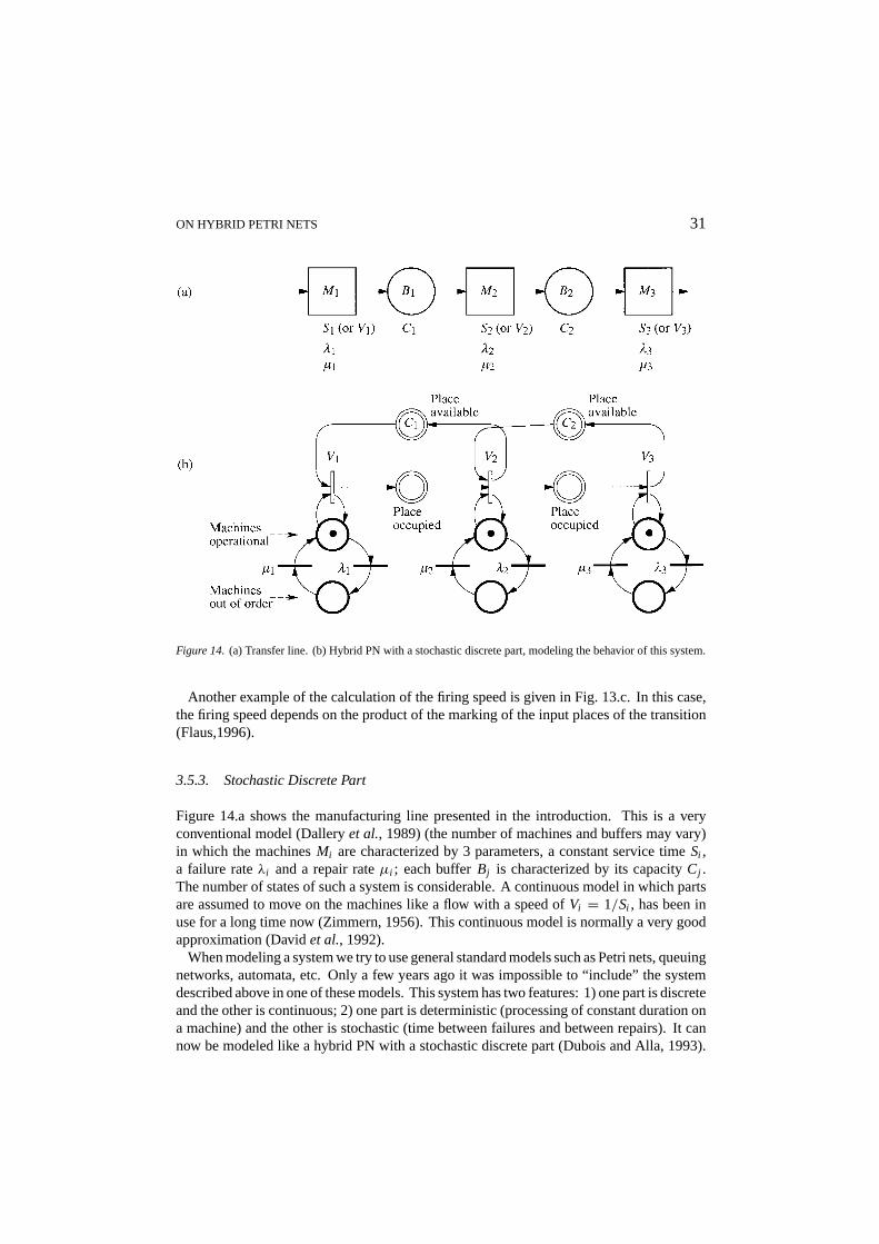
Figure 14. (a) Transfer line. (b) Hybrid PN with a stochastic discrete part, modeling the behavior of this system.

Another example of the calculation of the firing speed is given in Fig. 13.c. In this case,the firing speed depends on the product of the marking of the input places of the transition(Flaus,1996).

3.5.3. Stochastic Discrete Part

Figure 14.a shows the manufacturing line presented in the introduction. This is a veryconventional model (Dalleryet al., 1989) (the number of machines and buffers may vary)in which the machinesMi are characterized by 3 parameters, a constant service timeSi ,a failure rateλi and a repair rateµi ; each bufferBj is characterized by its capacityCj .The number of states of such a system is considerable. A continuous model in which partsare assumed to move on the machines like a flow with a speed ofVi = 1/Si , has been inuse for a long time now (Zimmern, 1956). This continuous model is normally a very goodapproximation (Davidet al., 1992).

When modeling a system we try to use general standard models such as Petri nets, queuingnetworks, automata, etc. Only a few years ago it was impossible to “include” the systemdescribed above in one of these models. This system has two features: 1) one part is discreteand the other is continuous; 2) one part is deterministic (processing of constant duration ona machine) and the other is stochastic (time between failures and between repairs). It cannow be modeled like a hybrid PN with a stochastic discrete part (Dubois and Alla, 1993).

32 DAVID AND ALLA

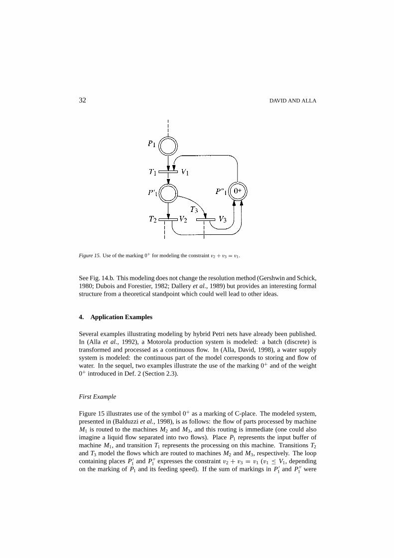
Figure 15.Use of the marking 0+ for modeling the constraintv2 + v3 = v1.

See Fig. 14.b. This modeling does not change the resolution method (Gershwin and Schick,1980; Dubois and Forestier, 1982; Dalleryet al., 1989) but provides an interesting formalstructure from a theoretical standpoint which could well lead to other ideas.

4. Application Examples

Several examples illustrating modeling by hybrid Petri nets have already been published.In (Alla et al., 1992), a Motorola production system is modeled: a batch (discrete) istransformed and processed as a continuous flow. In (Alla, David, 1998), a water supplysystem is modeled: the continuous part of the model corresponds to storing and flow ofwater. In the sequel, two examples illustrate the use of the marking 0+ and of the weight0+ introduced in Def. 2 (Section 2.3).

First Example

Figure 15 illustrates use of the symbol 0+ as a marking of C-place. The modeled system,presented in (Balduzziet al., 1998), is as follows: the flow of parts processed by machineM1 is routed to the machinesM2 and M3, and this routing is immediate (one could alsoimagine a liquid flow separated into two flows). PlaceP1 represents the input buffer ofmachineM1, and transitionT1 represents the processing on this machine. TransitionsT2

andT3 model the flows which are routed to machinesM2 andM3, respectively. The loopcontaining placesP′1 and P′′1 expresses the constraintv2 + v3 = v1 (v1 ≤ V1, dependingon the marking ofP1 and its feeding speed). If the sum of markings inP′1 and P′′1 were

ON HYBRID PETRI NETS 33

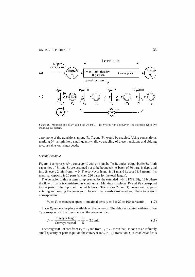
Figure 16. Modeling of a delay, using the weight 0+. (a) System with a conveyor. (b) Extended hybrid PNmodeling this system.

zero, none of the transitions amongT1, T2, andT3, would be enabled. Using conventionalmarking 0+, an infinitely small quantity, allows enabling of these transitions and abidingto constraints on firing speeds.

Second Example

Figure 16.a represents15 a conveyorC with an input bufferB1 and an output bufferB2 (bothcapacities ofB1 andB2 are assumed not to be bounded). A batch of 80 parts is depositedinto B1 every 2 min fromt = 0. The conveyor length is 11 m and its speed is 5 m/min. Itsmaximal capacity is 20 parts/m (i.e., 220 parts for the total length).

The behavior of this system is represented by the extended hybrid PN in Fig. 16.b wherethe flow of parts is considered as continuous. Markings of placesP2 and P5 correspondto the parts in the input and output buffers. TransitionsT3 and T4 correspond to partsentering and leaving the conveyor. The maximal speeds associated with these transitionscorrespond to:

V3 = V4 = conveyor speed×maximal density= 5× 20= 100 parts/min. (17)

PlaceP6 models the place available on the conveyor. The delay associated with transitionT2 corresponds to the time spent on the conveyor, i.e.,

d2 = Conveyor length

Conveyor speed= 11

5= 2.2 min. (18)

The weights 0+ of arcs fromP3 to T2 and fromT2 to P4 mean that: as soon as an infinitelysmall quantity of parts is put on the conveyor (i.e., inP3), transitionT2 is enabled and this

34 DAVID AND ALLA

quantity will be put at the end of the conveyor (i.e., inP4) when the timed2 has elapsed.Roughly speaking, this model corresponds to a “continuous firing of a discrete transition.”

Note that, if the conveyor speed changes, the values ofV3, V4, andd2, change immediatelyaccording to (17) and (18) (David and Caramihai, 2000).

5. Hybrid Petri Nets and Hybrid Automata

It has been shown in the previous sections that a hybrid PN inherits all the advantagesof PN models. It provides models designed in an intuitive way. Meanwhile, except forthe properties related to invariants, a quantitative analysis can be performed only via theconstruction of the evolution graph, which is a kind of simulation.

Hybrid automata are another tool for the modeling of hybrid dynamic systems. Severalprocedures have been proposed to analyze systems modeled by hybrid automata (Aluret al.,1995). Although this analysis is oriented mostly towards the verification of system speci-fications, these procedures may also be used for other analysis goals. Hybrid automata aredifficult to use for the modeling of complex systems. The goal of this section is to associatethe modeling power of hybrid PNs with the analysis power of hybrid automata by an auto-matic transformation from a hybrid PN into a hybrid automaton. This approach is similarto the approach combining stochastic PNs with Markov chains (automatic transformationfrom a stochastic PN into a Markov chain for which powerful analysis methods exist).

5.1. Hybrid Automata

In order to introduce the hybrid automaton model intuitively, let us consider an example.The water level in a tank is controled through a monitor, which continuously senses thewater level and turns a pumpon or off. The water level is represented by a variable h.When the pump isoff, the water level falls by 2 dm/min (decimeter per minute). When thepump ison, the water level rises by 1 dm/min. Suppose that initially the water level is 6dm and the pump is turnedon. We wish to keep the level of water between 1 and 12 dm.Moreover, there is a delay of 2 min from the moment that monitor signals the status of thepump until the change becomes effective. An extended hybrid PN describing the waterlevel monitor is shown in Fig. 17.a. PlacesP1 and P2 represent respectively the status onand off of the pump and placeP3 the level in the tank. TransitionT3 is continuously firedat speedv3 = V3 = 1. As soon asm3 = 10, transitionT2 is enabled; it is fired 2 minuteslater: T3 is no longer enabled andT4 becomes enabled. TransitionT1 will be enabled assoon asm3 < 5 . . .

It is easy to see that this model is natural since each node represents a physical entity. Thecorresponding hybrid automaton is given in Fig. 17.b. The construction of this model isless intuitive. It has four locations: in locationsl1 andl2, the pump is turnedon, in locationsl3 andl4, the pump isoff. The variabley models time delays,y is the time derivative ofy.Passing froml1 to l2 corresponds to enabling ofT2 (conditionh = 10); passing froml2 tol3 corresponds to firing ofT2 (conditiony = 2, andy is reset); and so on.

ON HYBRID PETRI NETS 35

Figure 17.Models of the water level monitor: (a) Hybrid PN, (b) Hybrid automaton.

Adopting the terminology of (Aluret al., 1995), a hybrid automaton is defined as follows(the examples refer to Fig. 17.b):

Definition7 A hybrid automaton is a seven-tupleH = 〈X, Q, ψ, Inv, A,Ev,As〉:X is a finite set of real-valuedvariables{xi }. We denote byx the vector of variables. The

values of all variables at a given moment define astate of variables(e.g.: X = {h, y}). Theset of states of variables is denoted byV .

Q is a finite set of vertices called locations (e.g.:Q = {l1, l2, l3, l4}).ψ is a function that assigns to each locationl ∈ Q a functionψi describing the evolution

of variables as a function of time (e.g. inl1: h = 1 andy = 0}).Inv is a function that assigns to each locationl ∈ Q a predicateInvl called theinvariant

of l (e.g. inl1: h ≤ 10}).A is a finite set of arcs called transitions. Each transitiona = (l , l ′) joins a source

locationl ∈ Q to a target locationl ′ ∈ Q (e.g.: A = {(l1, l2), (l2, l3), (l3, l4), (l4, l1)}). Anadditional arc without source location corresponds to initialization.

Ev is a function that assigns to each transitiona = (l , l ′), a predicateEva calledevent.The execution of transitiona = (l , l ′) is conditioned by the occurrence ofEva (e.g.:Ev(l2,l3)is “y = 2”).

Asis a function that assigns to each transitiona = (l , l ′) a relationAsa calledassignment.It is used to model the discrete changing of the values of continuous variables.Asa:x := g(x) (e.g.:As(l2,l3) corresponds to “y := 0”).

A particular class of hybrid automata is represented bylinear hybrid automata whichhave the following features:

1) The evolution functionsψl within a locationl are restricted to linear functions definedby a set of first-order differential equations of the formx = kl with kl denoting a constantvector.

36 DAVID AND ALLA

2) Each location invariantInvl and transition eventEva are defined by a conjunction oflinear inequalities overV of the formRx + c ≤ 0, whereR is a constant matrix,c is aconstant vector, andx ∈ V .

3) The transition assignmentAsa is defined by a relationx := V , wherex := V , for αx

is a linear term overV of the formR”x+c′, with R′ is a constant matrix andc′ is a constantvector.

5.2. From Hybrid PNs to Hybrid Automata

In order to systematize the change from hybrid PNs to hybrid automata, an algorithmhas been developed for the construction of the hybrid automaton associated with a hybridPN (Allam and Alla, 1998). Then quantitative analysis can be performed via the hybridautomaton model.

The hybrid PN functioning may be characterized by theevolution vector, made up of:1) theenabledD-transitions (more precisely, all the validations since, at a timet , a

transition may be enabled twice16 or more)2) thebalanceof the marking of the C-places (Def. 6 in Section 3.3.4).

According to Def. 5,one can notice that an IB-state implies an evolution vector. Hence,in the sequel, obtaining of the hybrid automaton is presented from the evolution graph.First, each IB-state is transformed into a location. Then, several locations correspondingto the same evolution vector may be merged.

In a hybrid PN (hence in an IB-state), the continuous variables are:1) the residual time to firing for every enabling of a timed D-transition;2) the marking of every continuous place.

Similarly, in every location, the continuous variables are:1) the time elapsed since enabling for every enabling of timed transition (the “delay

not yet elapsed” corresponds to the invariant of the location which is still satisfied, and“delay elapsed” is an event provoking a transition to another location;

2) the marking of every continuous place.Let us illustrate this transformation from the hybrid PN in Fig. 17.a. The corresponding

evolution graph is presented in Fig. 18.a. For construction of the hybrid automaton, thefollowing continuous variables are considered.

1) A variable yj for every timedD-transition Tj . WhenTj is enabled but not yetfired: y = 1. (in case of multiple enabling, new variables will be added when necessary:yj,1, yj,2, . . .).

2) A variablemi for everyC-place Pi ; at any timem= Bi (Section 3.3.3).For our example, the evolution vector is(y1, y2, m3) and the hybrid automaton obtained

from Fig. 18.a is shown in Fig. 18.b. At initial time,(y1, y2,m3) = (0,0,6).With the initial IB-state1, is associated the initial locationl1. NeitherT1 norT2 is enabled,

hencey1 − y2 = 0. Sincev3 = 1 andv4 = 0, B3 = m3 = 1. According to Fig. 18.a, thenext event provoking a change of IB-state is “m3 reaches the value 10”. This is the eventassociated with the transition froml1 to l2 in Fig. 18.b, and the invariant associated withl1is m3 ≤ 10.

ON HYBRID PETRI NETS 37

Figure 18. (a) Evolution graph for the hybrid PN in Fig. 17.a. (b) Corresponding hybrid automaton.

With the initial IB-state2, is associated the initial locationl2. In this locationy1 sinceT1

is enabled andm3 is still 1. The next event will bey1 = 2 (delay 2 associated with transitionT1 elapsed). Transition froml2 to l3 is performed and the value ofy1 is reset. And so on.

One can see in Fig. 18.b, that(y1, y2, m3) = (0,0,1) in both l1 andl5. In addition, theinvariant is the same and the event associated with the transitions tol2 is the same. Theselocations may be merged. It can be noticed that, after the merging, this automaton is iso-morphic to the automaton of Fig. 17.b. Only remaining difference: one clock y in Fig. 17.band two clocksy1 andy2 in Fig. 18.b. (y1 andy2 are never activated simultaneously).

6. Conclusion

Continuous systems together with their modeling, analysis and control have long providedresearch with subject matters. Modeling, analysis and control of discrete systems have

38 DAVID AND ALLA

undergone major developments in recent decades. General models such as automata, Petrinets and queuing networks are used with variants (extensions).

In recent years the need has emerged to consider systems which are partially continuousand partially discrete, in other words hybrid systems. To model such systems we coulduse certain modeling tools normally used for discrete systems. This has in fact beendone for automata (Aluret al., 1995), and for Petri nets as shown above (Le Bailet al.,1991). A software tool for modeling and simulation of continuous and hybrid PNs has beendeveloped.17

Petri nets are known to be powerful tools for modeling and analysis of discrete systems.The continuous and hybrid Petri nets, extensions of the basic model, allow modeling andanalysis of continuous and hybrid systems on the same conceptual basis. One can transforma timed hybrid PN into a hybrid automaton, then use the power analysis methods developedin the context of hybrid automata.

Notes

1. Since all the systems considered aredynamic ones, this adjective may be implicit. The expressiondiscretesystemsis used instead of ‘discrete event systems’ or ‘discrete event dynamic systems’, for homogeneity withthe expressions ‘continuous systems’ and ‘hybrid systems’ (indiscrete event systemsthe word event was addedto avoid confusion with discrete-time systems, sometimes called ‘discrete systems’ by abuse of language).

2. The terms “mark” and “token” are normally synonymous. We use the word “mark” to refer either to continuousor to discrete marking. The word “token” always has a discrete meaning.

3. In the text, two components of a vector are separated by a comma. Curly brackets represent a column vector,

i.e. (a,b) = [a b]T =[ab

].

4. R+ denotes the set of positive real numbers, including zero, andN denotes the set of natural numbers.

5. In (Alla and David, 1998), we have proposed for the case where the inhibitor arc has its origin at a continuousplace: enabling ifmi ≤ r and zero test forr = 0. This convention is not satisfactory since an arc with azeroweightusually corresponds to theabsenceof arc. This is the reason why we introduce now the concept ofinfinitely small weigth. It also allows to have the same conditionmi < r for either a D-place or a continuousplace (and no longermi ≤ r for the continuous case).

6. In previous papers, the authors have used the model “with reserved tokens” (like Fig. 6.b) for the discrete partof a hybrid PN. From now on, the model “without reserved tokens” (like Fig. 6.a) will be used. The modelingpower is the same for both models, i.e., any system modeled by one of these models can be modeled by theother one. Since, in a hybrid PN, the operations are essentially represented by continuous transitions, it maybe convenient to model the discrete part by the model without reserved tokens. Note that both models (withor without reservation of tokens) behave similarly as long as there is no conflict.

7. Note that the unit for a quantity of liquid is arbitrary: for example, the unit is 1 liter in Fig. 8.b but it could be,for example, 1 m3; in this case, we would havem3 = 0.060 m3 andV3 = 0.003 m3/sec (more generally, thebehavior is similar if all the markings and all the speeds are multiplied by an arbitrary positive value). On theother hand, the unit is not arbitrary for a number of discrete objects (number of parts in a buffer for example).

8. Obviously, these notions apply to pure continuous PN as well. Equ. (1) and (2) in Section 3.3.1 correspond tom3 = B3 = 2− 3 andm4 = B4 = 3− 2.

9. This is an extension to hybrid PNs of the definition given in (David and Alla, 1987) for the continuous PNs.

10. This means that, if a D-transitionTj becomes enabled (or becomes enabled once more) because the markingof a C-place in◦Tj has reached a sufficient value, a new IB-state is reached.

11. For example, in Fig. 10.c, IB-state3 can be reached either from2 or from5. In both cases,mC = (0,180).

12. For a D-place, this case corresponds to a first kind event.

ON HYBRID PETRI NETS 39

13. The choice represented by this rule was explicitly introduced in (David, 1997).

14. For some models, a transition firing speed may depend on the markings of the input places. For example, thevariable speed continuous PN (David and Alla, 1990) or the models in Fig. 13.b and c.

15. This example is inspired from an example in (Demongodin and Prunet, 1992).

16. For example, a D-transition with a single input D-place containing two tokens is enabled twice. If the delayassociated with the transition is not zero, the second enabling may occur between first enabling and first firing.

17. This software called SIRPHYCO is available at the address of one of the authors.

References

Alla, H., Cavaille, J.-B., Le Bail, J. and Bel, G. 1992. Les syst`emes de production par lot: une approchediscret-continu utilisant les r´eseaux de Petri hybrides.Symposium ADPM ’92. Paris.

Alla, H. and David, R. 1998. Continuous and Hybrid Petri Nets.Journal of Circuits, Systems & Computers8(1):159–188.

Allam, M. and Alla, H., 1997. Modelling production systems by hybrid automata and hybrid Petri nets.Conf. onControl of Industrial SystemsBelfort.

Allam, M. and Alla, H., 1998. From hybrid Petri nets to automata,JESA32(9-10): 1165–1185.Alur, R., Courcoubetis, C., Halwachs, N., Henzinger, T.A. , Ho, P.H., Nicollin, X. , Olivero, A., Sifakis, J. and

Yovine, S. 1995. The algorithmic analysis of hybrid systems.Theoretical Computer Science138: 3–34.Balduzzi, F., Giua, A. and Menga, G. 1998. Hybrid stochastic Petri nets: Firing dpeed computation and FMS

modelling.WODES ’98Gagliari.Brinkman, P. L. and Blaauboer, W. A. 1990. Timed continuous Petri nets: A tool for analysis and simulation of

discrete event systems.European Simulation SymposiumGhent.Charbonnier, F. 1993. Etude et r´esolution des conflits dans les r´eseaux de Petri hybrides. Internal Report, LAG,

INPG, Grenoble.Ciardo, G., Nicol, D. and Trivedi, K. S. 1997. Discrete-event simulation of fluid stochastic Petri nets.Petri Nets

& Performance Models PNPM’97Saint Malo, France, pp. 217–225.Cohen, G., Gaubert, S. and Quadrat, J.-P. 1995. Asymptotic throughput of continuous timed Petri nets.Conference

on Decision and ControlNew Orleans.Cohen, G., Gaubert, S. and Quadrat, J.-P. 1998.Algebraic System Analysis of Timed Petri Nets. Idempotency.

J. Gunawardena (Ed.). Cambridge Cambridge: University Press.Dallery, Y., David, R. and Xie, X. 1989. Approximate analysis of transfer lines with unreliable machines and

finite buffers.IEEE Trans. on Computers34(9): 943–953.David, R. 1997. Modeling of hybrid systems using continuous and hybrid Petri nets.Petri Nets & Performance

Models (PNPM’97). Saint Malo, France, pp. 47–58.David, R. and Alla, H. 1987. Continuous Petri nets.8th European Workshop on Application and Theory of Petri

NetsZaragoza.David, R. and Alla, H. 1990. Autonomous and timed continuous Petri nets.11th International Conference on

Application and Theory of Petri NetsParis, pp. 367–386.David, R. and Alla, H. 1992.Petri Nets and Grafcet: Tools for Modelling Discrete Event Systems. London:

Prentice Hall Int.David, R. and Caramihai, S. 2000. Modeling of delays on continuous flows thanks to extended hybrid Petri nets.

Int. Conf. an Automation of Mixed Proceses (ADPM 2000), Dortmund.David, R., Xie, X. and Dallery, Y. 1990. Properties of continuous models of transfer lines with unreliable machines

and finite buffers.IMA Journal of Math. Applied in Business & Industry6: 281–308.Demongodin, I. and Prunet, F. 1992. Extension of hybrid Petri nets to accumulation systems.IMACS Int. Symp.

on Mathematical Modelling and Scientific ComputingBangalore, India.Demongodin, I., Caradec, M. and Prunet, F. 1998. Fundamental concepts of analysis in batches Petri nets.Int.

IEEE Conf. on Systems, Man, and CyberneticsSan Diego, pp. 845–850.Demongodin, I. and Koussoulas, N.T. 1998. Differential Petri nets: Representing continuous systems in a discrete

event world.IEEE Transactions on Automatic Control38(4).Dubois, E. and Alla, H. 1993. Hybrid Petri nets with a stochastic discrete part.European Control Conference

Groningen.

40 DAVID AND ALLA

Dubois, E., Alla, H. and David, R. 1994. Continuous Petri net with maximal speeds depending on time.4th Int.Conf. of RPI, Computer Integrated Manufacturing and Automation TechnologyTroy, USA.

Dubois, D. and Forestier, J.-P. 1982. Productivit´e et en-cours moyens d’un ensemble de deux machines s´epareespar un stock.RAIRO Automatique16(2): 105–132.

Flaus, J.-M. 1996. Hybrid flow nets for batch process modelling.CESA 96, IEEE SMC. Lille.Gershwin, S. B. and Schick, I. C. 1980. Continuous Model of an Unreliable Two-Stage Material Flow System

With a finite Interstage Buffer.Technical report MIT LIDS-R- 1032.Halbwachs, N, Proy, Y. E. and Raymond, P. 1993. Verification of linear hybrid systems by means of convex

approximations.Proc. 5th Conf. on Decision and Compute-Aided Verification, LNCS 697Springer, pp. 220–228.

Le Bail, J., Alla, H. and David, R. 1991. Hybrid Petri nets.European Control ConferenceGrenoble, pp. 1472–1477.

Le Bail, J., Alla, H. and David, R. 1993. Asymptotic continuous Petri nets.Discrete Event Dynamic Systems:Theory and Applications2: 235–263.

Mandelbaum, A. and Chen, H. 1991. Discrete flow networks: Bottleneck analysis and fluid approximations.Math. Operations Research16: 408–446.

Murata, T. 1989. Petri Nets: Properties, Analysis and applications.Proceedings of the IEEE77(4): 541–580.Olsder, G. J. 1993. Synchronized Continuous Flow Systems. In:Discrete Event Systems: Modeling and Control,

S. Balemi, P. Kozak, & R. Smadinga (Eds.) Basel: Birkh¨auser Verlag.Peterson, J. L. 1981.Petri Net Theory and the Modelling of Systems. Prentice Hall.Pettersson, S. and Lennartson, B. 1995. Hybrid modelling focused on hybrid Petri nets.European Workshop on

Hybrid Systems. Grenoble, pp. 303–309.Ramchandani, C. 1973. Analysis of Asynchronous Concurrent Systems by Timed Petri Nets. Ph.D., MIT, USA.Sifakis, J. 1977. Use of Petri Nets for Performance Evaluation. In:Measuring, Modelling and Evaluating

Computer Systems, H. Beilner and E. Gelenbe (Eds.), North-Holland, pp. 75–93.Trivedi, K. S. and Kulkani, V. G. 1993. FSPNs: Fluid stochastic Petri nets.14th International Conference on

Application and Theory of Petri Nets, Chicago.Weiting, R. 1996. Hybrid high-level Nets.Proceedings of the Winter Simulation Conference, Coronado, USA,

pp. 848–855.Weiting, R. 1996. Modeling and Simulation of Hybrid Systems Using Hybrid High-Level Nets.Proceedings of

the 8th European Simulation Symposium, Genova, pp. 158–162.Zimmern, B. 1956. Etude de la propagation des arrÍts al´eatoires dans les chaÓnes de production.Revue de

Statistique Appliquee4: 85–104.