On International Financial Spillovers to Frontier...

On International Financial Spillovers to FrontierMarkets∗

Galin Todorov† Prasad Bidarkota‡

Florida International University

Fall 2010

Abstract

We explore the degree to which stock index returns and conditional volatility of 21frontier markets were affected by fluctuations on the American stock market betweenDecember 1st 2005 and January 15th 2010. We find weak, positive return spillovers fromUS to 17 frontier markets. For four countries, Jordan, Lebanon, Nigeria, and Kenya,we find weak negative return spillovers from the US, implying possible diversificationopportunities. For thirteen markets the influence of past local shocks is greater than theinfluence of current shocks from the US, and for sixteen markets local past volatility hasstronger impact than volatility from the US.

Key phrases: Frontier markets; Emerging markets; spillovers; contagion; time-varying volatility

JEL codes: F36, G15, C58∗Corresponding author: Galin Todorov, Department of Economics, Florida International University,

FL 33199, USA, telephone:(305) 348-2316, e-mail: [email protected].†Address: Department of Economics, Florida International University, FL 33199, USA, tele-

phone:(305) 348-2316, e-mail: [email protected].‡Address: Department of Economics, Florida International University, FL 33199, USA, tele-

phone:(305) 348-6362, e-mail: [email protected].

1. Introduction

The main issue investigated in this article is the extent to which contemporaneousreturns and conditional volatility of 21 frontier markets were affected by the fluctuationsin returns and conditional volatility on the American stock market during the periodbetween December 1st, 2005 and January 15th, 2010.

The World Bank defines emerging markets as markets for which GDP per capitafalls bellow a certain time-dependent hurdle. Frontier markets are defined as emergingmarkets that are investable, but have lower capitalization and market liquidity comparedto the more developed emerging markets.

Financial spillovers exist due to real economic and financial ties between worldeconomies. As a result of the existence of such ties, new information arising in onecountry affects not only local returns and volatility, but also the returns and volatility ofassets traded on other markets. The impact of a change in returns of one stock marketon the returns of another stock market is defined as returns spillovers, and the impactof a change in returns volatility of one stock market on the returns volatility of anotherstock market is defined as volatility spillovers. The new information may be absorbedimmediately by other markets, or with a delay, depending on the presence and numberof informed investors, information asymmetry, level of market liquidity, existence of feedback traders and herding behavior, high transaction costs and other potential marketspecific factors. The magnitude and speed of spillovers provide valuable insight into thenature and swiftness of dissemination of such new information among countries. Thesize of spillovers reflects how global investors feel about news, as well as their appraisalof its impact on asset prices across markets.

In order to travel across borders, information needs transmission channels. In theshort run, asset price changes are the primary channel for transmission of financial shocksacross borders. Owing to the dependence of frontier markets on common bank creditorsand cross market portfolio re-balancing by investment funds, financial markets and in-stitutions have been shown to act as a major tool for cross-border shock transmission(Kodres and Pritsker (2002), Calvo (1999), Pritsker (2001)). Detailed review of spillovertransmission channels is offered by Pritsker (2001), and Kaminsky and Reinhart (2002).

The great majority of theoretical and empirical work has so far been concentrated onexploring spillovers among the mature and more developed emerging markets. However,the growing size and importance of frontier markets naturally draw considerable interestfrom investors, policy makers, and academics alike. In this study we extend the existingliterature by analyzing the extent to which small markets are vulnerable to shocks fromthe USA, as represented by the returns and volatility spillovers from the US market to21 frontier stock markets.

The exposure of the smallest developing markets to financial shocks from US is amatter of substantial concern for international investors. Frontier markets are often

1

considered very risky. That however, might not stem from those markets not being fun-damentally sound; it might just be that investors do not know much about them. Thisstudy may provide financiers with further information about potential investment andportfolio diversification opportunities in those 21 small economies. Direct investment,project risk evaluation, cost of capital calculation, asset pricing and allocation, in addi-tion to the development of hedging techniques can potentially benefit from this articleas well.

Policy makers may take advantage of this study since understanding inter-marketconnections could provide for more informed decisions, improve macroeconomic man-agement, as well as advance their ability to time, predict, and evaluate susceptibilityof a country to shocks from abroad. Improved assessment of the nature and origin ofa financial shock and possible subsequent economic downturn may facilitate the adap-tation of more appropriate anti-crisis techniques and thus alleviate, or at least shorten,the suffering of those most affected by the deterioration of economic conditions.

Exploration of potential inter-market linkages may also aid academics in sheddingmore light on the outcome of market liberalization on capital flows and mobility. En-hanced awareness of market co-movement may expand their understanding of the signif-icance of the structure and potential effects of free cash flows as well as any subsequentrestrictions. Furthermore, this study may assist academics in forecasting and evaluatingthe reaction of international financial markets to global and local shocks, as well as inachieving deeper understanding of the shock transmission mechanisms.

Last but not least, when analyzing these economies, we should not be confused withthe meaning of the word small: it refers only to the per capita income, not to thenumber of people living in those economies. The population of Argentina alone is closeto 40 million, Romanian population is over 20 million, and in any one of those smalleconomies live people struggling to survive every day. This paper will try to answerthe question of how quickly, and how badly were those markets affected by the recenteconomic downturn and may even provide some insights about future macroeconomicpolicy course.

The evidence presented in this article suggests that spillovers from USA to frontiermarkets are rather weak, albeit statistically significant. One possible implication is thatthe global economic downturn worked its way in these countries through a differenttransmission channel, or that the economic deterioration in those frontier markets is duemainly to an idiosyncratic country specific shock. Furthermore, our results put forwardthe notion that it is not the lagged US market returns that have influence, rather itis the expected US market returns that have impact on frontier market returns. Theinference is that despite different opening hours, non synchronous trading, stale orders,information asymmetry and other possible small market inefficiencies, the frontier mar-kets absorb news from the USA almost immediately at the time of the news release. This

2

leads us to the conjecture that frontier market might not at all be inefficient, rather,their real and financial sectors might be resilient to influence from the US. From theperspective of a global financier, this finding means that there might exist some diver-sification benefits from investing in these developing economies. From the perspectiveof a developing country policy maker it means that a potential increase in capital flowsfrom the US does not necessarily increase local market volatility even in times when theUS economy is deteriorating.

In section 2 of this article we proceed with relevant literature review on financialspillovers; in section 3 we present the data and offer some descriptive statistics; section4 develops the empirical models; in section 5 we report and discuss our results; section6 concludes.

2. Literature Review

Interdependency and correlations among world financial markets have been investi-gated since the mid 1960s, however, this area of international finance gained most ofits popularity after the stock market crash of 1987 with King and Wadhwani (1990) es-tablishing the unidirectional impact of the US stock returns on other markets, Hamao,Masulis, and Ng (1990) confirming the unidirectional impact of US market return volatil-ity, and Eun and Shim (1989) examining the interdependency across nine stock markets.Harvey (1995) found that adding emerging market assets to a portfolio significantly en-hances its opportunity set. He showed that the exposure of emerging markets to commonfactors is low and that it is more likely that local variables have stronger influence thando global variables. Aggarwal, Inclan, and Leal (1999) support the last claim, report-ing that important local events in each country, rather than global factors, tend tobe associated with sudden changes in volatility. Bekaert and Harvey (1997) ascertainthat capital market liberalization increases return spillovers across markets but does notaffect market volatility, while Tanizaki and Hamori (2009) determine that market volatil-ity is increasing in the amount of information available. From asset allocation point ofview, increasing spillover effects are generally associated with an increase in cross mar-ket correlations and thus reduced opportunities for cross border portfolio diversification(Bekaert, Harvey (2000), (2003)).

The literature on financial spillovers received a significant boost after the 1997 Asiancrisis. Sola, Spagnolo, and Spagnolo (2001) find unidirectional volatility spillovers fromThailand, the country where the crisis originated, to most of the countries in the region.Caporale, Cippollini, and Spagnolo (2003) confirm unidirectional spillovers in returnsfrom the Thai stock market. Kim (2005) and Gebka and Serwa (2006) affirm the signif-icant influence of the American market on the Asian markets at all times, and Gebkaand Serwa (2007) find significant contemporaneous spillovers from the USA during thesame period.

3

Egert and Kocenda (2009), as well as Fadhlaoui, Bellalh, Dherry, and Zonaouri (2009) find some evidence for short term spillovers, but no long term relations, betweendeveloped and emerging markets of Central and Eastern Europe. Yu and Hassan (2006)and Al-Kulaib, Najand, and Mashayekh (2009) find no spillovers from the USA to theMiddle East, North African, and Gulf Cooperation Countries, while Chen, Firt, andRui (2000) suggest high correlation of Latin American countries with world markets andthus limited potential for portfolio diversification.

Psillaki, and Margaritis (2008) claim no long term relationship, but some short terminterdependence between the USA stock market and the French and German stockmarkets. Pollard, Sapra, and Canarella (2007), on the other hand, find significant impactfrom both the USA market returns and volatility on the Canadian and Mexican markets.Beirne, Caporale, Schulze-Ghatts and Spagnolo (2008) suggest that mature marketsinfluence the conditional variances in many emerging markets. Sgherri and Galesi (2009)clarify for 27 countries that asset prices are the main channel of transmission of financialshocks internationally in the short run.

3. Data

In this article we use daily MSCI Barra index closing prices to explore the returnson the US stock market and 21 frontier markets for the period from December 1st, 2005to January 15th, 2010. The daily returns for each country are calculated as follows:

Rit = ln(Pit/Pi(t-1))

where Pit is the value for each country’s index closing price at time t.We choose daily data since it will better account for the stock market dynamics

and provides greater insight on cross-market interactions.The countries included are:Argentina, Bahrain, Bulgaria, Croatia, Estonia, Jordan, Kazakhstan, Kenya, Kuwait,Lebanon, Mauritius, Nigeria, Oman, Pakistan, Qatar, Romania, Saudi Arabia, Slovenia,Sri Lanka, Tunisia, and United Arab Emirates. The countries and duration of the periodunder study are chosen such that the longest index series is available for the greatestnumber of countries. Lithuania, Serbia, Ukraine, Bangladesh, Trinidad and Tobago,Jamaica, Botswana and Ghana are also defined by the World Bank as frontier markets,but are not included in this study due to lack of data for a sufficiently long period.

MSCI indices are established consistently across countries and thus provide an ad-equate ground for exploration of inter-market relations. They are value-weighted andcalculated with the dividends reinvested. In order to avoid double counting, stock pricesof companies set up abroad are not included. All indices are in US dollars, whichprovides additional comparability across markets and implicitly takes care of currencymarket effects.

4

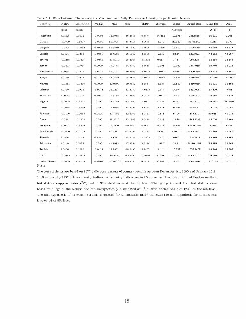
Descriptive statistics for the US and 21 frontier markets are reported in Table 1.1.The statistics include annualized arithmetic and geometric means, median, maximum,and minimum geometric returns for each country, as well as skewness, excess kurtosis,Jarque-Bera, Ljung-Box (6), and Arch (6) test statistics. Annualized arithmetic meanreturns range from 0.09% for Kazakhstan to -0.08% for UAE and -0.0003% for the USmarket. The annualized geometric mean returns range from 0.2529% for Kazakhstan to-0.3458% for UAE and -0.0236 % for the USA. The annualized standard deviation of ge-ometric returns ranges from 8.013% for Kazakhstan to 2.7907% for Tunisia and 4.0558%for the USA. The mean returns are low as anticipated, considering that the period un-der study incorporates the economic downturn of 2007-2009. The standard deviation isquite high for the frontier markets, as expected (Harvey (1995)). It could be resultingfrom various liquidity effects or heterogeneous information sets of investors. The stan-dard deviation is quite high for the US returns as well, representing the turmoil on theUS market. The range of geometric returns is quite narrow, amid the high standarddeviation, and not that distant from the US market returns implying that the frontiermarkets might be well integrated with the rest of the world, despite the possibility forsegmentation. The null hypothesis for no skewness is rejected at 5% significance levelfor Kazakhstan, Kenya, Mauritius, and Sri Lanka; the values for skewness are positivefor all four countries. All countries display high and significant excess kurtosis, possiblydue to to time variation of conditional variance, as well as significant non normality asrepresented by the Jarque-Bera test statistic. The returns for all countries are highlyserially correlated at 6 lags. No statistically significant auto-correlation is exhibited bythe returns from Argentina, Bahrain, Kuwait, Romania, and Saudi Arabia.

The summary statistics provided in Table 1.1 offer an insight that contrasts withthe existing literature. The average returns and standard deviation for frontier marketsare not much different than for the USA. One implication could be that these markets,however young, may not represent a considerable diversification opportunity for foreigninvestors. This could be due to the fact that these markets are economically and finan-cially integrated with the US market. Another possibility is that the frontier marketindices under study may be comprised mainly of internationally operating companies forwhich shocks from the US have greater impact than local market shocks. These indicesmay or may not truly represent the financial and economic sectors of the respectivecountries, in which case we can infer nothing about integration.

4. Methodology

In the Data section we have demonstrated the presence of substantial deviationsfrom normality and considerable leptokurtosis in the country data series. One type ofmodels that can capture these characteristics is the Arch type models. Arch type modelswere first introduced by Engle (1982) to account for the influence of changing volatility

5

in time series. Engle (1982) represents the conditional variance as a linear function oflagged squared residuals. The basic specification for an Arch model has the form

Rt = a+ ut

ut = h1/2t zt

zt ∼ iidN(0, 1)

ht = b0 + b1u2t-1

Because only one lag of squared residual is incorporated, a model such as the aboveis called Arch(1).

Bollerslev (1986) modified the Arch model by allowing lagged values of the condi-tional variance to be incorporated in the conditional variance equation. A basic GARCH(p,q) model describes the conditional variance as

Rt = a+ ut

ut = h1/2t zt

zt ∼ iidN(0, 1)

ht = c0 +p∑

i=1ciu

2t-i +

q∑i=1

biht-1

In order to avoid negative conditional variance the parameters of the variance equa-tion must be non-negative, c0 > 0, ci ≥ 0, bi ≥ 0.

GARCH models are shown to better account for fat tails and volatility clustering re-sulting from time variation in conditional volatility. It has also been found that GARCH(1,1) specification is the most appropriate for capturing these effects ( Bollerslev (1986),Enders (2001), Hamilton (1994)).

In this paper we utilize two separate models to describe the evolution of returns inemerging markets. First, we utilize univariate GARCH (1,1) model to specify marketreturns as a function of own past values; then we specify a bivariate model that accountsfor the impact of returns and volatility from the US market.

4.1 UNIVARIATE MODEL

6

The univariate model is defined as follows:

Rjt = b0 +

12∑i=1

biRjt-i + ujt

ujt =√hjtzt

zt ∼ iidN(0, 1)

hjt = a0 + a1uj2t-1 + a2h

jt-1

Rjt− log index return for country j.

b0− the portion of the returns explained by factors other than shocks and pastreturns.

bi−parameter representing the impact of own country lagged returns on current re-turns.

ujt−represents the unexplained portion of the country returns.hjt−conditional variance for country j. It is interpreted as a proxy for market senti-

ment towards news originating within the country.a0−GARCH regression constant; represents the portion of the conditional volatility

explained by factors other than the lagged excess returns and lagged conditional volatil-ity. It is the portion of the market sentiment that is due neither to market sentimenttowards news in the past, nor to excess returns.

a1−parameter representing the impact of lagged excess returns.a2−parameter representing the impact of market sentiment towards past news orig-

inating within the country .The above specification is estimated for returns from all 21 frontier markets, as well

as the United States. The number of lagged returns included in the best-fitting modelis determined using the Schwarz-Bayesian Criterion (SBC).

Appendix 1 presents details on the estimated factor loadings of the univariate modelsfor each country and Table 1.2 reports a summary of the best-fitting models; discussionis offered in section 5.1.

4.2 BIVARIATE MODELIn this section we upgrade the best-fitting univariate model to a bivariate model

in order to account for the effect of the USA returns and conditional volatility on themarket returns of individual countries. The bivariate model is defined as follows:

7

Rjt = b0 +

12∑i=1

biRjt-i +

12∑i=0

ciRust-i + ujt

ujt =√hjtzt

zt ∼ iidN(0, 1)


jt-1 + a3h

ust + a4h

ust-1

where the variables and parameters additional to the univariate model are definedas follows:

Rust-i−log index returns for the US market representing shocks originating from the

USA. When i = 0 we consider shocks on the US market that occur on the same day asthe returns of the country under study. When i > 0, we consider past shocks to the USmarket.

ci−parameter represents return spillovers from the US market to the market of thecountry under study. When i = 0, c0 represents the impact on returns of contempo-raneous US shocks, and when i > 0, ci represents the impact on returns of past USshocks.

hust −conditional variance for the USA market. It is interpreted as a proxy for marketsentiment of traders on the USA market towards news originating in the USA and isderived from the univariate model of US market returns.

a3& a4 parameters representing the impact of market sentiment of US investorstowards contemporaneous news originating in the USA on the sentiment of the individualfrontier country investors.

We choose to consider a GARCH model without any asymmetry, although theasymmetric impact on financial series volatility of negative news has long been studied(Glosten, Jagannathan, Runkle (1993)). For emerging markets, however, no asymmetryeffects have been shown and any potential asymmetry is assumed to enter through theidiosyncratic shock ujt (Bekaert, Harvey, and Ng(2005)).

The above specification is estimated for returns from all 21 frontier markets. Thenumber of lagged US returns included in the best-fitting bivariate model is determinedusing the Schwarz-Bayesian Criterion (SBC).

Appendix 2 presents details on the estimated factor loadings of the bivariate modelsfor each country and Table 1.3 reports a summary of the best-fitting models; discussion

8

is offered in section 5.2.4.3 HYPOTHESIS TESTINGIn this text we investigate whether the country’s own lag market return effects bi

and the US current and lagged market return effects ci have any statistical significance.This is done by using LR test to explore the null hypothesis of whether bi = 0 andci = 0, where the number of lags i of local and US returns is determined using the SBC.Further, we apply the LR test to examine the impact of the volatility spillover effectsa3, and a4; the hypotheses tested are a3 = 0 and a4 = 0. We also study the possibilityfor homoscedasticity of the error term; we do that by applying the LR test to the nullhypothesis: a1 = a2 = a3 = a4 = 0. At the 5% significance level and the null forhomoscedasticity is rejected in favor of the Garch specification.

The test statistics derived from the significance tests performed on the best-fittingbivariate models are presented in Table 1.4 and a summary is reported in Table 1.5.

5. Empirical Results

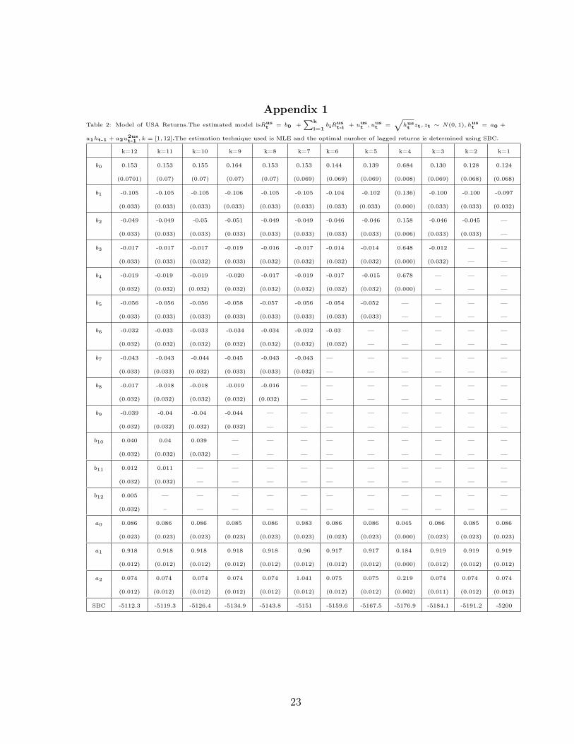
5.1 UNIVARIATE MODELAppendix 1 presents detailed results from the estimation of univariate models for

the US and each of the 21 frontier markets. For each country we investigate 12 models,where each model is specified based on a different number of included own countrylagged returns. The number of lagged returns under consideration ranges from 1 to 12,and the best-fitting model is determined using the Schwarz-Bayesian Criterion (SBC).A summary of the coefficients from the estimation the best-fitting univariate models forall countries is presented in Table 1.2

According to the Schwarz-Bayesian criterion (SBC), for the US and 20 out of the 21frontier markets, with Kenya being the only exception, the best-fitting univariate modelis one that includes only one period lagged home returns, and is defined as follows:

Rjt = b0 + b1R

jt-1 + ujt

ujt =√hjtzt

zt ∼ iidN(0, 1)


jt-1

One possible implication that can be inferred from this finding is that the influenceof shocks from home is no more persistent for the frontier markets than for the USA

9

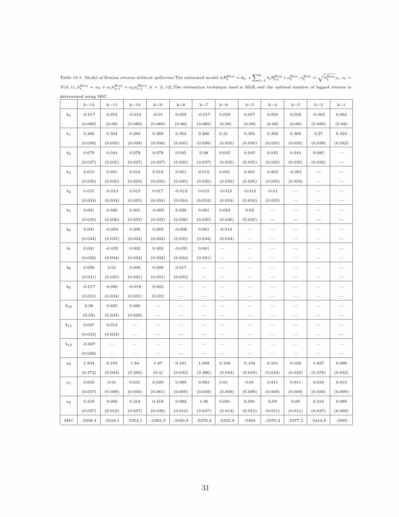
market.For Kenya, the best-fitting univariate model is

Rjt = b0 + b1R

jt-1 + b2R

jt-2 + ujt

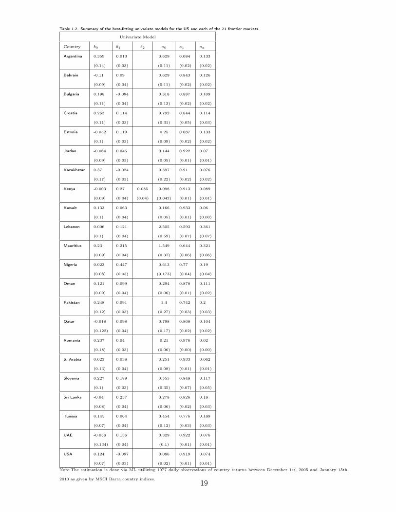
with the other equations as described above.Table 1.2 suggests magnitude of the regression constant b0 greater than 0.1 for more

than half of the countries. The presence of a significant positive constant means theunconditional expected returns are positive. This suggests optimistic outlook of investorsabout the future. The constant captures latent factors determining the mean of thereturns, as well as unobservable variables affecting the returns, but omitted in our model.The existence of such factors may be due to potential unavailability of data other thanlagged returns, or poor quality of the available data. Potential latent factors could bepolitical instability, government regulations, corruption, international compatibility ofaccounting standards, as well as different regional factors.

For several countries, Table 1.2 reports lower magnitude of the constant, relative totheir peers. The relatively low magnitude of the constant implies low, or even negativemean returns for these countries, low or negative expected returns, and thus relativelypessimistic prospects about the future. The low magnitude may also imply that thereis more data available for these countries, as well as better quality of the data, whichis fully captured by the index returns. One implication of such possibility could bethat markets in these countries are more efficient, which results in the weaker presenceof latent factors and unobservable variables. Another possibility is that while homemarkets as a whole may be unable to incorporate all relevant information, the returns ofthe companies having most weight in the MSCI index are resilient to local factors otherthan past returns. This could be because the companies in question operate mostlyinternationally, there is more and better quality data available for them, or they arelarge enough to not be affected by home market processes.

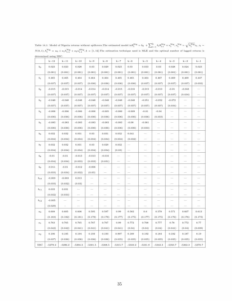
According to Table 1.2, for most of the countries the influence of past returns bi

is below 0.1. For eight countries, the impact of past returns is greater than 0.1. Thegreater the impact of past returns, the longer it takes for those markets to evaluate thefull effect of past shocks. One possibility is that the economies of these countries are notthat well diversified, and a shock to one sector trickles to other sectors and that trickletakes time to be evaluated.

The magnitude of the variance constant a0 for most of the countries is between zeroand one, as presented in Table 1.2. For the USA the value of the variance constant is0.086, which is the lowest for all countries. Since the US market has been shown tobe efficient in incorporating information (Fama (1998)), the effect of any unobservablevariables or latent factors is absorbed immediately through a change in returns. For

10

the frontier markets, the lowest constant value is for Kenyan returns: 0.098. For fourmarkets the magnitude of the constant is greater than one. Those markets are Argentina(1.711), Lebanon (2.5), Mauritius (1.549) , and Pakistan (1.4).

Table 1.2 further indicates the influence of one period lagged events on current mar-ket sentiment a1 is between 0.5 and 1, for almost all countries, including the US (0.919).Considering that the period under study incorporates periods of great market turbulenceand uncertainty, it seems reasonable to assume that the impact of any past news is beingcontinuously reassessed. A high coefficient of impact may imply not only abundance ofinformation, but also abundance of important information, such as announcement ofstructural reforms, or lack there of, announcements of new government policies or regu-lations, outdated statistical information. The only country with relatively low impact ofpast local news is Estonia (0.087). Considering that Estonia is a small, export orientedeconomy, it is realistic to believe that the index data is composed of predominantly ex-port oriented companies, for which local information is relatively unimportant relativeto global news and thus the coefficient of impact of past local news is relatively low.

5.2 BIVARIATE MODELAppendix 2 presents detailed results from the estimation of bivariate models for

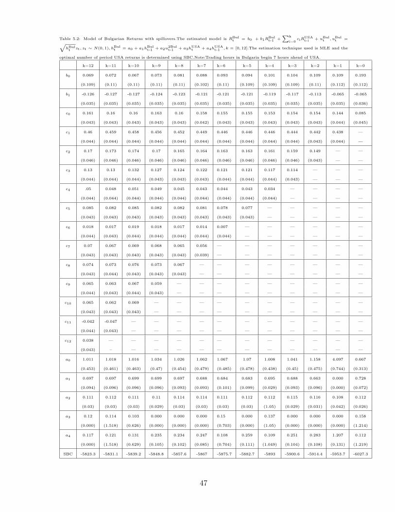
each of the 21 frontier markets and a summary of the results is presented in Table 1.3.For each country we investigate 13 models, where each model is specified based on adifferent number of included US lagged returns. The number of lagged returns underconsideration ranges from 0 to 12, and the best-fitting model is determined using theSchwarz-Bayesian Criterion (SBC). According to the Schwarz-Bayesian criterion (SBC),for 16 out of the 21 frontier markets the best-fitting bivariate model is one that includesonly contemporaneous US market returns and no US lagged returns. The model isspecified as follows:

Rjt = b0 + b1R

jt-1 + coR

ust + ujt

ujt =√hjtzt

zt ∼ iidN(0, 1)


jt-1 + a3h

ust + a4h

ust-1

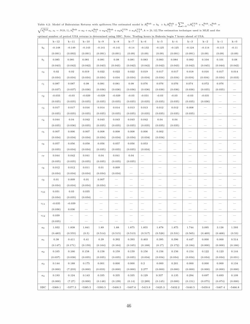
where hust is derived from the uni-variate model for US returns.For four countries, Bahrain, Kuwait, Oman, and Tunisia, Table 1.3 suggests the

bivariate model contains one period US lagged returns, along with the contemporaneous

11

returns:Rj

t = b0 + b1Rjt-1 + c0R

ust + c1R

ust-1 + ujt

with the other equations the same as above.For the Kenyan market, the bivariate model contains two period lagged domestic

returns and contemporaneous returns from the US. This model is as follows:

Rjt = b0 + b1R

jt-1 + b2R

jt-2 + c0R

ust + ujt

with other equations as above.Figures plotting the observed returns, as well as the returns predicted by the best-

fitting bivariate model for each country are presented in Appendix 3. Each figure revealsthe progression of the plotted variables over time and illustrates the degree to which thevariance of the observed returns is explained by our best-fitting models.

5.3 DISCUSSION OF SPILLOVERSThe center piece of the bivariate model, summarized in Table 1.3, is the investigation

of return and volatility spillovers from the US to the local markets as measured by theparameters c0, a3, and a4. The greatest return spillovers from the USA are to Argentina(0.957), Kazakhstan (0.237), and Romania (0.329). For majority of the countries the im-pact coefficients fall between 0.0 and 0.1, with 4 markets experiencing negative spillovers:Jordan (-0.021), Lebanon (-0.059), Nigeria (-0.027), and Kenya (-0.028) at lag one.

For Argentina, Kazakhstan, and Romania the high impact coefficients may indicatedeep economic inter-dependence between those countries and the US, rather than fi-nancial relations only. The economies of these four countries are predominantly exportoriented and trade relations might be one reason for economic integration. If the tradeexport of those economies is predominantly to the USA, then they might not be welldiversified and thus vulnerable to shocks from the American market. One implicationis that in these four countries, international investors may find little or no scope fordiversification. Not such is the situation with the markets experiencing negative impactfrom the US: Jordan, Lebanon, Nigeria, and Kenya. The negative relation between theUS returns and returns in those countries implies low degree of inter-dependence be-tween local economies and the US economy and thus presence of possible diversificationopportunities from the standpoint of international portfolio managers. From a policymaker’s point of view, those countries seem resilient to shocks from the US market.One implication is that downturn in USA should not be blamed for recession in thosecountries, and any economic slow down is more likely to be “home grown” rather than“imported” from US, at least not through this channel.

It is interesting to note that although the local and US market returns occur on thesame date, the markets under study open before the US market and have little or nooverlap in trading hours. Most of those markets open seven or more hours before the US

12

market opens, with the exception being Argentina opening one hour ahead, Nigeria andTunisia five hours ahead, and Slovenia six hours ahead. One important implication ofthis finding is that it might not be the actual US returns that matter, but the expectedUS returns. Any announcements made in the USA after closing of the stock exchangeson day one, and before opening on day two, are absorbed by the US market on daytwo. Throughout the trading day on local frontier markets, investors observe thoseannouncements, and incorporate them in their asset valuation immediately, while theyonly get incorporated in the US returns on the next trading day in the US, which inmost cases starts just after closing of local markets. To better describe such a situation,we could say that it is the US overnight returns that affect the local markets, ratherthan the actual daily returns, where the overnight returns are defined as the change inprice between closing on day one and opening on day two. The overnight returns formthe expected returns, and are reflected in the US daily returns on the next day, so thosereturns seem to affect the local market returns despite the fact that local markets mayclose for the day before the US market opens. Similar discussion and more details onthe international transmission of overnight returns can be found in Hamao, Masulis, andNg (1994), Lin, Engle, and Ito (1994), and Baur and Jung (2006).

For thirteen of the twenty one frontier markets, Table 1.3 reports the impact coeffi-cient of lagged home returns b1 is greater than the impact coefficient of the current USreturns c0. This implies that for the period under study for those markets, the averageimpact of domestic shocks is stronger than the average impact of shocks from the USmarket. This suggests that the economies of those countries may be less vulnerable toUS market deterioration relative to their peers. The opposite is true for the remainingeight markets. For those, the average influence of shocks from the US is greater thanthe average influence of domestic shocks, and their economies may be more vulnerableto US market shocks relative to their peers.

The impact coefficients a3 and a4 representing volatility spillovers give us the scaleof transmission of market sentiment from the US stock market to the local markets ofthe countries under study. In accordance with literature on emerging markets, Table1.3 reports that volatility spillovers are weaker relative to return spillovers. Currentperiod spillover parameter a3 for most of the countries falls between 0.00 and 0.05.The low magnitude of impact coefficients imply weak, albeit statistically significant,cross-market transmission of market sentiment from the US market. The degree oftransmission of market sentiment might also be indicative of the presence of feed backtrading and herding behavior. The low parameter values imply very limited presence ofthose inefficiencies. Exception are Argentina (0.084), Bahrain (0.134), Bulgaria (0.158),Croatia (0.103), Mauritius (0.33), Romania (1.836), and Saudi Arabia (0.122). Similarlyfor one period lagged spillovers, majority of the countries fall in the range between 0.00and 0.05. Exceptions are Bahrain (0.109), Bulgaria (0.112), Kenya (0.119), Lebanon

13

(0.066), Nigeria (0.161), Romania (0.436), and Saudi Arabia (0.28). For these markets,and especially for Romania, there is stronger indication for cross-border transmission ofmarket sentiment and thus more prominent presence of herding behavior and feed backtrading.

It is worth exploring whether the market sentiment of local market investors hjt isaffected mostly by the current and lagged market sentiment of US investors hUSt andhUSt-1 , or by the local investors’ sentiment towards domestic lagged events hjt-1. For mostof the countries, Table 1.3 indicates magnitude of the impact coefficient of lagged ownmarket news a1 between 0.5 and 1.0. This result implies that past local news and localmarket sentiment on average have stronger impact on local investors compared to bothcurrent and lagged news from the US market. For several countries like Kenya, Lebanon,Nigeria, Romania, and Saudi Arabia, the coefficient capturing the effect of local newson market sentiment is not significantly different from null. For these countries, thesentiment of US investors is more important than local factors. For five countries, thevalue of variance constant a0 is quite high: 6.033 for Kenya, 8.194 for Lebanon, 6.081 forNigeria, 9.675 for Romania, and 22.271 for Saudi Arabia. Implication is that for thesefrontier markets there is significant influence of international and domestic factors otherthan those included in the Garch specification. One possible explanation is that thoseeconomies are mostly export oriented and their exports are sensitive to a wide varietyof international factors.

To summarize, for half of the countries, the influence of local shocks and marketsentiment is stronger than the influence stemming from the US market. The interde-pendence of most of the frontier markets with the US market is weak, albeit significant.The weak interdependence can be attributed to fluctuations in the relative significanceof market specific shocks versus shocks from the US. When shocks from US dominate do-mestic shocks, markets will move closer together and will appear more integrated. Whendomestic shocks dominate shocks from the US, the markets will move further apart andwill appear more segmented. In addition, frontier markets could be underrepresented inglobal portfolios and thus be insulated from portfolio re-balancing. Last but not least,the US and frontier market indices may have significantly different structure which mayfurther reduce the cross-border market co-movement. Furthermore, we find that localmarkets absorb information from US as soon as it appears which implies frontier marketsare highly informationally efficient.

6. ConclusionIn this article we examine the degree to which the returns and conditional volatility of

21 frontier markets were affected by the fluctuations in returns and conditional volatilityof the American stock market during the period between December 1st, 2005 and Jan-uary 15th, 2010. Using Schwarz-Bayesian criterion we find that for seventeen countriesthe best-fitting model is one that includes only the contemporaneous US returns, and for

14

four countries, the best-fitting model includes one period lagged US returns as well. Wefind weak, albeit significant, mostly positive return spillovers from the US market. Forfour countries, Jordan, Lebanon, Nigeria, and Kenya, we find weak negative spillovers,implying possible diversification opportunities. For thirteen markets, the influence ofpast local shocks is greater than the influence of current shocks from the US, and forsixteen markets local past volatility has stronger impact than volatility from US.

We find that frontier markets incorporate new information as soon as it arrives andfor most of the countries local information is weighted heavier relative to informationfrom the USA.

The research presented in this article may be extended using time-varying parametertechniques to better account for market dynamics and possible switching dominanceovertime of domestic and US shocks. Other extensions could be the investigation of theeffects of incomplete information and fat tails on market interdependence, as well as anempirical assessment of various shock transmission channels across frontier markets.

15

References

Aggarwal R, Inclan C, Leal R. Volatility in emerging stock markets. Journal ofFinancial and Quantitative Analysis. 1999;34(1):33.

Alkulaib Yaser A., Najand Mohammad MA. Dynamic linkages among equity marketsin the Middle East and North African countries. Journal of Multinational FinancialManagement. 2009;19:43-53.

Baur, Dirk, Jung RC. Return and volatility linkages between the US and the Germanstock market. Journal of International Money and Finance 2006;25:598-613.

Beirne J, Caporale G, Schulze-Ghattas M, Spagnolo N. Volatility spillovers and con-tagion from mature to emerging stock markets. IMF WP08-286; 2009.

Bekaert G, Harvey C, Ng A. Market integration and contagion. Journal of Business.2005;78(1).

Bekaert G, Harvey C. Emerging markets finance. Journal of Empirical Finance.2003;10(1-2):3–56.

Bekaert G, Harvey C. Foreign speculators and emerging equity markets. Journal ofFinance. 2000;55(2):565–613.

Bekaert, Geert HC. Emerging equity market volatility. Journal of Financial Eco-nomics. 1997;43:29-77.

Bollerslev T. Generalized autoregressive conditional heteroskedasticity. Journal ofEconometrics. 1986;31(3):307–327.

Calvo G. Contagion in emerging markets: When Wall Street is a carrier. IEA Con-ference Volume Series.Vol 136. Citeseer; 2004:81–94.

Caporale G, Pittis N, Spagnolo N. Volatility transmission and financial crises. Jour-nal of Economics and Finance. 2006;30(3):376–390.

Chen G, Firth M, Meng Rui O. Stock market linkages: evidence from Latin America.Journal of Banking & Finance. 2002;26(6):1113–1141.

Egert B, Kocenda E. Interdependence between Eastern and Western European stockmarkets: evidence from intraday data. Economic Systems. 2007;31(2):184–203.

Enders W. Applied econometric time series. Wiley & Sons;1995.Engle R. Autoregressive conditional heteroskedasicity with estimates of the variance

of U.K. inflation. Econometrica. 1982;50(4):987-1008.Eun CS, Shim S. International transmission of stock market movements. Journal of

Financial and Quantitative Analysis. 1989;24(2):241.Fama E. Market efficiency, long-term returns, and behavioral finance. Journal of

Financial Economics. 1998;49(3):283-306.Fadhlaoui Kais, Bellalah Makram, Dherry Armand ZM. An empirical examination of

international diversification benefits in central european emerging markets. InternationalJournal of Business. 2009;14(2).

16

Gebka B, Serwa D. Are financial spillovers stable across regimes? Evidence from the1997 Asian crisis. Journal of International Financial Markets, Institutions and Money.2006;16(4):301-317.

Gebka B, Serwa D. Inter-regional spillovers between emerging capital markets aroundthe world. Research in International Business and Finance. 2007;21:203-221.

Hamao Y, Masulis R, Ng V. Correlations in price changes and volatility across in-ternational stock markets. Review of Financial Studies. 1990;3(2):281–307.

Hamilton J. Time series analysis. Princeton Univ Pr; 1994.Harvey C. Predictable risk and returns in emerging markets. Review of Financial

Studies. 1995;8(3):773–816.Kaminsky G, Reinhart C. Financial markets in times of stress. Journal of Develop-

ment Economics. 2002;69(2):451–470.Kim S. The spillover effects of US and Japanese public information news in advanced

Asia-Pacific stock markets. Pacific-Basin Finance Journal. 2003;11(5):611–630.King, M. , Wadhawani S. Transmission of volatility between stock markets. Review

of Financial Studies. 1990;3(1):5-33.Kodres, Laura E, Pritsker M. A rational expectations model of financial contagion.

Journal of Finance. 2002;57(2):769-799.Lin W, Engle R, Ito T. Do bulls and bears move across borders? International trans-

mission of stock returns and volatility. Review of Financial Studies. 1994;7(3):507–538.Pollard S, Sapra S, Canarella G. Asymmetry and spillover effects in the North Amer-

ican equity markets. econstor.eu. 2007;1:323-343.Pritsker M. The channels for financial contagion. International financial contagion.

2001;(202):67–95.Psillaki M, Margaritis D. Long-run interdependence and dynamic linkages in inter-

national stock markets: evidence from France Germany and the US. Journal of Money,Investment and Banking. 2008;(4).

Sgherri S, Galesi A. Regional financial spillovers across Europe: a global VAR anal-ysis. IMF WP09-23; 2009.

Sola M, Spagnolo F, Spagnolo N. A test for volatility spillovers. Economics Letters.2002;76(1):77–84.

Tanizaki H, Hamori S. Volatility transmission between Japan, UK and USA in dailystock returns. Empirical Economics. 2009.

Yu, Jung-Suk, Hassan M. Kabir. Global and regional integration of the Middle Eastand North African (MENA) stock markets. The Quarterly Review of Economics andFinance. 2008;48:482-504.

17

Table 1.1: Distributional Characteristics of Annualized Daily Percentage Country Logarithmic Returns.

Country Aritm. Geometric Median Max Min St.Dev. Skewness Excess Jarque-Bera Ljung-Box Arch

Mean Mean Kurtosis Q (6) (6)

Argentina 0.0132 0.0402 0.0993 32.6988 -46.2513 6.3874 -0.7162 10.375 2532.538 10.211 9.908

Bahrain -0.0709 -0.2817 0.0000 28.9765 -45.3414 4.0973 -1.969 27.112 26785.910 7.029 6.779

Bulgaria -0.0425 -0.1962 0.1092 28.6710 -46.1532 5.4928 -1.656 15.502 7506.549 48.598 44.373

Croatia 0.0424 0.1266 0.0850 26.6783 -26.1957 4.5298 -0.139 8.566 1393.671 44.203 44.097

Estonia -0.0285 -0.1407 -0.0845 31.5919 -25.2044 5.1833 0.067 7.717 999.328 15.594 15.548

Jordan -0.0493 -0.1997 0.0000 19.9778 -24.5732 3.7938 -0.798 10.049 2343.659 16.740 16.012

Kazakhstan 0.0935 0.2529 6.6272 47.0791 -36.4983 8.0123 0.308 * 8.876 1566.270 14.933 14.857

Kenya 0.0140 0.0293 0.0143 24.9572 -25.4871 3.9877 0.389 * 11.818 3516.884 177.778 152.377

Kuwait -0.0311 -0.1405 0.0000 22.0500 -29.9682 4.4587 -1.124 11.522 3486.069 11.221 11.358

Lebanon 0.0330 0.0905 6.9078 26.0267 -41.2237 4.6815 -0.144 14.974 6461.628 37.326 40.03

Mauritius 0.0648 0.2141 6.4973 27.3738 -21.9885 4.0508 0.161 * 11.364 3144.202 29.664 27.879

Nigeria -0.0008 -0.0252 0.000 14.3145 -23.1930 4.0417 -0.339 6.227 487.871 386.863 312.699

Oman -0.0045 -0.0399 0.000 27.1075 -44.4726 4.1464 -1.441 23.956 20080.11 24.028 29.007

Pakistan -0.0196 -0.1056 0.0404 21.7455 -32.4033 4.9821 -0.573 5.709 388.471 60.615. 49.038

Qatar -0.0241 -0.1228 0.000 28.3712 -33.1923 5.0448 -0.633 10.79 2795.2385 15.020 16.169

Romania 0.0032 -0.0505 0.000 31.5860 -79.6922 6.7691 -1.622 21.999 16669.7203 7.505 7.222

Saudi Arabia -0.0466 -0.2136 0.000 40.8917 -37.5188 5.6521 -0.97 13.0370 4689.7826 11.998 12.382

Slovenia 0.0276 0.0753 0.1253 23.8831 -24.8745 4.3279 -0.419 9.043 1670.1873 35.569 38.793

Sri Lanka 0.0149 0.0332 0.000 41.8982 -17.8501 3.9139 1.99 * 24.32 21110.1407 85.355 74.464

Tunisia 0.0436 0.1486 0.0411 22.7851 -18.0495 2.7907 0.11 10.719 2676.3479 19.266 19.886

UAE -0.0813 -0.3458 0.000 46.9438 -43.5286 5.9894 -0.601 13.015 4565.6213 34.686 30.529

United States -0.0003 -0.0236 0.1446 27.8273 -23.9746 4.0558 -0.242 12.003 3648.3631 35.8725 35.637

Note:

The test statistics are based on 1077 daily observations of country returns between December 1st, 2005 and January 15th,

2010 as given by MSCI Barra country indices. All country indices are in US currency. The distribution of the Jarque-Bera

test statistics approximates q2(2), with 5.99 critical value at the 5% level. The Ljung-Box and Arch test statistics are

based on 6 lags of the returns and are asymptotically distributed as q2(6) with critical value of 12.59 at the 5% level.

The null hypothesis of no excess kurtosis is rejected for all countries and * indicates the null hypothesis for no skewness

is rejected at 5% level.

18

Table 1.2. Summary of the best-fitting univariate models for the US and each of the 21 frontier markets.

Univariate Model

Country b0 b1 b2 a0 a1 aa

Argentina 0.359 0.013 0.629 0.084 0.133

(0.14) (0.03) (0.11) (0.02) (0.02)

Bahrain -0.11 0.09 0.629 0.843 0.126

(0.09) (0.04) (0.11) (0.02) (0.02)

Bulgaria 0.198 -0.084 0.318 0.887 0.109

(0.11) (0.04) (0.13) (0.02) (0.02)

Croatia 0.263 0.114 0.792 0.844 0.114

(0.11) (0.03) (0.31) (0.05) (0.03)

Estonia -0.052 0.119 0.25 0.087 0.133

(0.1) (0.03) (0.09) (0.02) (0.02)

Jordan -0.064 0.045 0.144 0.922 0.07

(0.09) (0.03) (0.05) (0.01) (0.01)

Kazakhstan 0.37 -0.024 0.597 0.91 0.076

(0.17) (0.03) (0.22) (0.02) (0.02)

Kenya -0.003 0.27 0.085 0.098 0.913 0.089

(0.09) (0.04) (0.04) (0.042) (0.01) (0.01)

Kuwait 0.133 0.063 0.166 0.933 0.06

(0.1) (0.04) (0.05) (0.01) (0.00)

Lebanon 0.006 0.121 2.505 0.593 0.361

(0.1) (0.04) (0.59) (0.07) (0.07)

Mauritius 0.23 0.215 1.549 0.644 0.321

(0.09) (0.04) (0.37) (0.06) (0.06)

Nigeria 0.023 0.447 0.613 0.77 0.19

(0.08) (0.03) (0.173) (0.04) (0.04)

Oman 0.121 0.099 0.294 0.878 0.111

(0.09) (0.04) (0.06) (0.01) (0.02)

Pakistan 0.248 0.091 1.4 0.742 0.2

(0.12) (0.03) (0.27) (0.03) (0.03)

Qatar -0.018 0.098 0.798 0.868 0.104

(0.122) (0.04) (0.17) (0.02) (0.02)

Romania 0.237 0.04 0.21 0.976 0.02

(0.18) (0.03) (0.06) (0.00) (0.00)

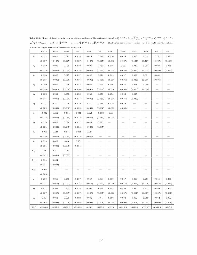
S. Arabia 0.023 0.038 0.251 0.933 0.062

(0.13) (0.04) (0.08) (0.01) (0.01)

Slovenia 0.227 0.189 0.555 0.848 0.117

(0.1) (0.03) (0.35) (0.07) (0.05)

Sri Lanka -0.04 0.237 0.278 0.826 0.18

(0.08) (0.04) (0.06) (0.02) (0.03)

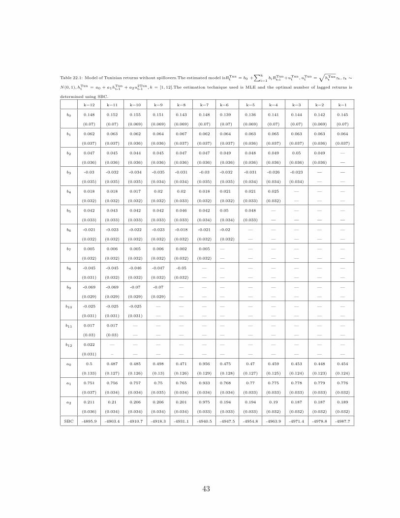
Tunisia 0.145 0.064 0.454 0.776 0.189

(0.07) (0.04) (0.12) (0.03) (0.03)

UAE -0.058 0.136 0.329 0.922 0.076

(0.134) (0.04) (0.1) (0.01) (0.01)

USA 0.124 -0.097 0.086 0.919 0.074

(0.07) (0.03) (0.02) (0.01) (0.01)

Note:The estimation is done via ML utilizing 1077 daily observations of country returns between December 1st, 2005 and January 15th,

2010 as given by MSCI Barra country indices.19

Table 1.3: Summary of the best-fitting bivariate models for each of the 21 frontier markets.

Bivariate Model

Country b0 b1 b2 c0 c1 a0 a1 a2 a3 a4

Argentina 0.18 0.111 0.957 1.31 0.72 0.185 0.084 0.017

(0.12) (0.03) (0.05) (0.44) (0.07) (0.04) (0.314) (0.31)

Bahrain -0.115 0.101 0.017 0.076 3.126 0.000 0.123 0.000 0.693

(0.09) (0.04) (0.03) (0.04) (0.47) (0.00) (0.03) (0.00) (0.07)

Bulgaria 0.193 -0.065 0.085 0.67 0.728 0.112 0.158 0.112

(0.11) (0.04) (0.05) (0.31) (0.07) (0.03) (1.21) (1.219)

Croatia 0.246 0.107 0.13 1.672 0.676 0.155 0.103 0.000

(0.11) (0.04) (0.04) (0.54) (0.09) (0.05) (0.05) (0.00)

Estonia -0.023 0.131 0.111 0.17 0.83 0.14 0.039 0.04

(0.1) (0.03) (0.04) (0.12) (0.03) (0.02) (0.65) (0.65)

Jordan -0.067 0.044 -0.02 0.144 0.91 0.073 0.009 0.000

(0.09) (0.03) (0.03) (0.07) (0.02) (0.01) (0.01) (0.00)

Kazakhstan 0.349 -0.003 0.237 0.613 0.897 0.081 0.016 0.016

(0.17) (0.03) (0.06) (0.23) (0.02) (0.02) (0.00) (0.00)

Kenya -0.023 0.216 0.106 -0.028 6.039 0.000 0.409 0.001 0.119

(0.09) (0.03) (0.03) (0.03) (0.47) (0.00) (0.06) (0.02) (0.04)

Kuwait -0.014 0.064 0.003 0.077 6.71 0.000 0.031 0.000 0.781

(0.11) (0.04) (0.04) (0.04) (0.64) (0.00) (0.02) (0.00) (0.08)

Lebanon -0.36 -0.249 -0.059 8.194 0.000 1.088 0.000 0.066

(0.1) (0.03) (0.03) (0.87) (0.00) (0.13) (0.00) (0.042)

Mauritius 0.249 0.213 0.037 2.095 0.196 0.512 0.33 0.008

(0.08) (0.04) (0.03) (0.48) (0.06) (0.08) (0.00) (0.000)

Nigeria 0.022 0.49 -0.027 6.081 0.000 0.261 0.000 0.161

(0.09) (0.03) (0.03) (0.57) (0.00) (0.05) (0.00) (0.05)

Oman 0.071 0.111 -0.004 0.141 3.216 0.000 0.081 0.000 0.686

(0.09) (0.04) (0.03) (0.03) (0.04) (0.03) (0.03) (0.00) (0.07)

Pakistan 0.248 0.092 0.019 1.394 0.743 0.197 0.000 0.000

(0.12) (0.03) (0.02) (0.27) (0.03) (0.03) (0.00) (0.000)

Qatar -0.049 0.098 0.003 0.762 0.838 0.103 0.01 0.05

(0.12) (0.04) (0.04) (0.22) (0.03) (0.02) (0.00) (0.00)

Romania 0.171 0.07 0.329 9.675 0.000 0.114 1.836 0.431

(0.16) (0.03) (0.06) (1.59) (0.00) (0.04) (0.00) (0.00)

S. Arabia -0.117 0.04 0.086 2.271 0.001 0.072 0.122 0.28

(0.16) (0.04) (0.05) (1.30) (0.00) (0.02) (1.19) (1.19)

Slovenia 0.208 0.198 0.096 1.479 0.575 0.13 0.174 0.056

(0.1) (0.03) (0.04) (0.47) (0.12) (0.03) (2.34) (2.35)

Sri Lanka -0.041 0.237 0.061 0.382 0.732 0.24 0.018 0.017

(0.08) (0.04) (0.03) (0.11) (0.05) (0.05) (0.19) (0.19)

Tunisia 0.161 0.121 0.078 0.148 4.458 0.000 0.217 0.000 0.093

(0.08) (0.04) (0.02) (0.02) (0.39) (0.00) (0.05) (0.00) (0.03)

UAE -0.056 0.137 0.01 0.351 0.902 0.082 0.016 0.018

(0.14) (0.04) (0.05) (0.14) (0.02) (0.01) (0.3) (0.3)

Note:

The estimation is done via ML utilizing 1077 daily observations of country returns between December 1st, 2005 and

January 15th, 2010 as given by MSCI Barra country indices. All country indices are in US currency.

20

Table 1.4: LR tests of the coefficients of the best-fitting model of country returns with spillovers

LR Test Statistics

H0 : b1 = 0 c0 = 0 b1 = c0 = 0 a1=0 a2 = 0 a3 = 0 a4 = 0 a1 = a2 = a3 = a4 = 0

Country (j) (i-max, = a3 = a4 = 0

k-max)

Argentina (1,0) 15.542 441.81 378.168 45.838 111.427 151.02 151.021 377.43 151.01

Bahrain (1,1) 17.298 59.84 8.361 12.06 41.827 0.000 0.000 490.67 47.007

Croatia (1,0) 6.45 17.72 15.49 9.829 65.825 145.408 137.52 274.80 11.7

Estonia (1,0) 14.28 90.08 15.058 87.4 188.37 240.467 156.271 415.184 176.49

Jordan (1,0) 1.775 131.9 6.53 131.31 164.18 277.79 236.84 308.99 254.78

Kazakhstan (1,0) 0.007 222.99 43.426 210.28 318.16 275.26 210.289 419.04 2.59

Kenya (2,0) 34.71 0.98 56.725 0.001 189.78 197.29 208.93 302.201 296.35

Kuwait (1,1) 131.03 127.67 134.81 127.667 107.009 13.9128 13.913 413.16 11.74

Lebanon (1,0) 20.727 4.817 24.035 231.38 175.19 0.000 3.693 194.68 3.69

Mauritius (1,0) 25.654 68.24 25.819 61.41 167.823 155.321 380.89 380.89 155.321

Nigeria (1,0) 70.09 0.987 70.627 141.529 69.32 24.623 22.75 152.57 27.15

Oman (1,1) 94.101 84.22 110.95 84.205 98.039 0.000 27.357 546.074 31.65

Pakistan (1,0) 7.075 159.12 164.158 158.159 306.26 158.74 167.93 329.607 120.159

Qatar (1,0) 7.216 62.04 14.047 61.505 94.74 265.28 218.365 302.54 241.17

Romania (1,0) 4.118 27.85 30.25 52.062 25.066 224.98 0.000 248.50 235.974

Saudi Arabia (1,0) 433.71 433.923 434.24 433.596 45.866 61.087 63.19 99.118 62.99

Slovenia (1,0) 102.705 74.62 105.613 69.86 29.55 187.87 199.37 422.66 21.19

Sri Lanka (1,0) 419.88 405.52 425.45 402.99 301.43 462.115 343.95 520.03 11.34

Tunisia (1,1) 275.33 266.84 176.33 262.76 139.11 30.08 26.03 178.93 7.405

UAE (1,0) 424.52 386.46 424.63 386.22 196.28 315.98 294.64 331.04 302.81

Note:

The best-fitting model is RJt = b0 +

∑i-max=2i=1 biR

Jt-1 +

∑k-max=1k=0 ckR

USAt-1 + uJt , u

Jt =

√hJt zt, zt ∼ N(0, 1), hJt =

a0 + a1hJt-1 + a2u2Jt-1 + a3hUSAt + a4hUSAt-1 .The testing technique used is LR, where the LR statistic is approximately chi-

squared. The critical value with 1 degree of freedom and p-value=.05 is 3.84;with 2 degrees of freedom and p-value=.05

the critical value is 5.99; with 3 degrees of freedom and p-value =.05 the critical value is 7.82; and with 4 degrees of

freedom and p-value=.05 the dritical value is 9.49 .

21

Table 1.5: Summary of hypothesis test results

Country Spillovers Spillovers from Current Spillovers from one-period Garch

in Mean Period US Volatility Lag US Volatility

Argentina yes yes yes yes

Bahrain yes no no yes

Bulgaria yes yes yes yes

Croatia yes yes yes yes

Estonia yes yes yes yes

Jordan yes yes yes yes

Kazakhstan yes yes yes yes

Kenya yes yes yes yes

Kuwait yes yes yes yes

Lebanon yes no yes yes

Mauritius yes yes yes yes

Nigeria no yes yes yes

Oman yes no yes yes

Pakistan yes yes yes yes

Qatar yes yes yes yes

Romania yes yes no yes

S. Arabia yes yes yes yes

Slovenia yes yes yes yes

Sri Lanka yes yes yes yes

Tunisia yes yes yes yes

UAE yes yes yes yes

Note:

Presence of garch effects, and return and volatility spillovers for each of the 21 frontier markets.

22

Appendix 1Table 2: Model of USA Returns.The estimated model isRus

t = b0 +∑k

i=1biR

ust-i + uus

t , uust =

√hust zt, zt ∼ N(0, 1), hus

t = a0 +

a1ht-1 + a2u2ust-1 , k = [1, 12].The estimation technique used is MLE and the optimal number of lagged returns is determined using SBC.

k=12 k=11 k=10 k=9 k=8 k=7 k=6 k=5 k=4 k=3 k=2 k=1

b0 0.153 0.153 0.155 0.164 0.153 0.153 0.144 0.139 0.684 0.130 0.128 0.124

(0.0701) (0.07) (0.07) (0.07) (0.07) (0.069) (0.069) (0.069) (0.008) (0.069) (0.068) (0.068)

b1 -0.105 -0.105 -0.105 -0.106 -0.105 -0.105 -0.104 -0.102 (0.136) -0.100 -0.100 -0.097

(0.033) (0.033) (0.033) (0.033) (0.033) (0.033) (0.033) (0.033) (0.000) (0.033) (0.033) (0.032)

b2 -0.049 -0.049 -0.05 -0.051 -0.049 -0.049 -0.046 -0.046 0.158 -0.046 -0.045 —

(0.033) (0.033) (0.033) (0.033) (0.033) (0.033) (0.033) (0.033) (0.006) (0.033) (0.033) —

b3 -0.017 -0.017 -0.017 -0.019 -0.016 -0.017 -0.014 -0.014 0.648 -0.012 — —

(0.033) (0.033) (0.032) (0.033) (0.032) (0.032) (0.032) (0.032) (0.000) (0.032) — —

b4 -0.019 -0.019 -0.019 -0.020 -0.017 -0.019 -0.017 -0.015 0.678 — — —

(0.032) (0.032) (0.032) (0.032) (0.032) (0.032) (0.032) (0.032) (0.000) — — —

b5 -0.056 -0.056 -0.056 -0.058 -0.057 -0.056 -0.054 -0.052 — — — —

(0.033) (0.033) (0.033) (0.033) (0.033) (0.033) (0.033) (0.033) — — — —

b6 -0.032 -0.033 -0.033 -0.034 -0.034 -0.032 -0.03 — — — — —

(0.032) (0.032) (0.032) (0.032) (0.032) (0.032) (0.032) — — — — —

b7 -0.043 -0.043 -0.044 -0.045 -0.043 -0.043 — — — — — —

(0.033) (0.033) (0.032) (0.033) (0.033) (0.032) — — — — — —

b8 -0.017 -0.018 -0.018 -0.019 -0.016 — — — — — — —

(0.032) (0.032) (0.032) (0.032) (0.032) — — — — — — —

b9 -0.039 -0.04 -0.04 -0.044 — — — — — — — —

(0.032) (0.032) (0.032) (0.032) — — — — — — — —

b10 0.040 0.04 0.039 — — — — — — — — —

(0.032) (0.032) (0.032) — — — — — — — — —

b11 0.012 0.011 — — — — — — — — — —

(0.032) (0.032) — — — — — — — — — —

b12 0.005 — — — — — — — — — — —

(0.032) – — — — — — — — — — —

a0 0.086 0.086 0.086 0.085 0.086 0.983 0.086 0.086 0.045 0.086 0.085 0.086

(0.023) (0.023) (0.023) (0.023) (0.023) (0.023) (0.023) (0.023) (0.000) (0.023) (0.023) (0.023)

a1 0.918 0.918 0.918 0.918 0.918 0.96 0.917 0.917 0.184 0.919 0.919 0.919

(0.012) (0.012) (0.012) (0.012) (0.012) (0.012) (0.012) (0.012) (0.000) (0.012) (0.012) (0.012)

a2 0.074 0.074 0.074 0.074 0.074 1.041 0.075 0.075 0.219 0.074 0.074 0.074

(0.012) (0.012) (0.012) (0.012) (0.012) (0.012) (0.012) (0.012) (0.002) (0.011) (0.012) (0.012)

SBC -5112.3 -5119.3 -5126.4 -5134.9 -5143.8 -5151 -5159.6 -5167.5 -5176.9 -5184.1 -5191.2 -5200

23

Table 3.1: Model of Argentinian returns without spillovers.The estimated model isRArgt = b0 +

∑k

i=1biR

Argt-i + u

Argt , u

Argt =√

hArgt zt, zt ∼ N(0, 1), h

Argt = a0 + a1h

Argt-1 + a2u

2Argt-1 , k = [1, 12].The estimation technique used is MLE and the optimal number

of lagged returns is determined using SBC.

k=12 k=11 k=10 k=9 k=8 k=7 k=6 k=5 k=4 k=3 k=2 k=1

b0 0.388 0.388 0.375 0.388 0.386 0.388 0.379 0.382 0.374 0.373 0.362 0.359

(0.149) (0.148) (0.148) (0.148) (0.147) (0.147) (0.147) (0.146) (0.146) (0.145) (0.144) (0.144)

b1 0.014 0.013 0.014 0.015 0.014 0.014 0.014 0.014 0.014 0.014 0.014 0.013

(0.034) (0.033) (0.034) (0.034) (0.034) (0.033) (0.034) (0.033) (0.033) (0.033) (0.033) (0.033)

b2 -0.012 -0.012 -0.013 -0.013 -0.013 -0.012 -0.012 -0.013 -0.012 -0.013 -0.013 —

(0.033) (0.033) (0.033) (0.033) (0.033) (0.032) (0.033) (0.033) (0.033) (0.033) (0.033) —

b3 -0.024 -0.024 -0.026 -0.027 -0.027 -0.024 -0.027 -0.027 -0.028 -0.028 — —

(0.033) (0.032) (0.033) (0.033) (0.033) (0.033) (0.033) (0.033) (0.033) (0.033) — —

b4 -0.004 -0.004 -0.003 -0.003 -0.003 -0.004 -0.002 -0.002 -0.003 — — —

(0.032) (0.032) (0.032) (0.032) (0.032) (0.032) (0.032) (0.032) (0.032) — — —

b5 -0.02 -0.02 -0.018 -0.02 -0.02 -0.02 -0.02 -0.02 — — — —

(0.033) (0.032) (0.033) (0.033) (0.033) (0.033) (0.033) (0.033) — — — —

b6 0.008 0.008 0.01 0.01 0.01 0.008 0.009 — — — — —

(0.031) (0.031) (0.031) (0.031) (0.031) (0.031) (0.03) — — — — —

b7 -0.017 -0.017 -0.02 -0.018 -0.018 -0.017 — — — — — —

(0.032) (0.032) (0.032) (0.032) (0.032) (0.032) — — — — — —

b8 0.002 0.002 0.005 0.005 0.005 — — — — — — —

(0.031) (0.031) (0.031) (0.031) (0.031) — — — — — — —

b9 -0.009 -0.009 -0.01 -0.009 — — — — — — — —

(0.03) (0.03) (0.03) (0.03) — — — — — — — —

b10 0.033 0.033 0.034 — — — — — — — — —

(0.03) (0.03) (0.03) — — — — — — — — —

b11 -0.07 -0.07 — — — — — — — — — —

(0.03) (0.03) — — — — — — — — — —

b12 0.002 — — — — — — — — — — —

(0.03) – — — — — — — — — — —

a0 1.725 1.724 1.7 1.715 1.716 1.00 1.7 1.703 1.73 1.729 1.718 1.711

(0.457) (0.458) (0.45) (0.449) (0.447) (0.448) (0.442) (0.442) (0.448) (0.448) (0.443) (0.44)

a1 0.81 0.81 0.811 0.81 0.81 0.99 0.81 0.811 0.809 0.809 0.81 0.81

(0.038) (0.038) (0.037) (0.037) (0.037) (0.037) (0.037) (0.037) (0.037) (0.037) (0.037) (0.036)

a2 0.139 0.139 0.139 0.14 0.14 1.033 0.14 0.139 0.141 0.14 0.14 0.14

(0.03) (0.03) (0.03) (0.03) (0.03) (0.03) (0.03) (0.03) (0.03) (0.03) (0.03) (0.03)

SBC -6448 -6455 -6467.9 -6476.2 -6483.2 -6490 -6497.5 -6504.6 -6512 -6518 -6526 -6533

24

Table 4.1: Model of Bahrainian returns without spillovers.The estimated model isRBaht = b0 +

∑k

i=1biR

Baht-i + uBah

t , uBaht =√

hBaht zt, zt ∼ N(0, 1), hBah

t = a0 + a1hBaht-1 + a2u

2Baht-1 , k = [1, 12].The estimation technique used is MLE and the optimal number


k=12 k=11 k=10 k=9 k=8 k=7 k=6 k=5 k=4 k=3 k=2 k=1

b0 -0.115 -0.114 -0.11 -0.105 -0.1 -0.115 -0.099 -0.097 -0.107 -0.107 -0.11 -0.11

(0.09) (0.09) (0.09) (0.09) (0.091) (0.09) (0.09) (0.09) (0.092) (0.092) (0.092) (0.092)

b1 0.082 0.083 0.085 0.088 0.089 0.082 0.089 0.09 0.09 0.09 0.089 0.09

(0.041) (0.04) (0.041) (0.041) (0.04) (0.04) (0.041) (0.04) (0.041) (0.041) (0.04) (0.04)

b2 -0.005 -0.004 0.000 0.000 0.003 -0.005 0.004 0.005 0.007 0.006 0.007 —

(0.04) (0.04) (0.04) (0.04) (0.04) (0.04) (0.04) (0.04) (0.04) (0.04) (0.04) —

b3 0.009 0.011 0.011 0.011 0.013 0.009 0.014 0.014 0.013 0.017 — —

(0.038) (0.038) (0.038) (0.038) (0.038) (0.038) (0.038) (0.038) (0.038) (0.038) — —

b4 0.023 0.022 0.022 0.024 0.026 0.023 0.027 0.027 0.035 — — —

(0.039) (0.039) (0.039) (0.039) (0.039) (0.039) (0.039) (0.039) (0.039) — — —

b5 0.053 0.053 0.053 0.055 0.058 0.053 0.058 0.064 — — — —

(0.035) (0.035) (0.035) (0.036) (0.036) (0.036) (0.036) (0.035) — — — —

b6 0.05 0.05 0.053 0.054 0.056 0.05 0.057 — — — — —

(0.037) (0.037) (0.037) (0.037) (0.037) (0.037) (0.037) — — — — —

b7 0.01 0.01 0.011 0.011 0.008 0.01 — — — — — —

(0.036) (0.036) (0.036) (0.036) (0.036) (0.036) — — — — — —

b8 0.013 0.013 0.013 0.011 0.017 — — — — — — —

(0.036) (0.036) (0.036) (0.036) (0.036) — — — — — — —

b9 0.075 0.076 0.075 0.078 — — — — — — — —

(0.035) (0.035) (0.035) (0.035) — — — — — — — —

b10 0.036 0.036 0.039 — — — — — — — — —

(0.033) (0.033) (0.033) — — — — — — — — —

b11 0.043 0.044 — — — — — — — — — —

(0.035) (0.035) — — — — — — — — — —

b12 0.011 — — — — — — — — — — —

(0.034) – — — — — — — — — — —

a0 0.624 0.6234 0.631 0.624 0.627 1.012 0.624 0.625 0.630 0.628 0.631 0.629

(0.104) (0.104) (0.106) (0.106) (0.107) (0.107) (0.106) (0.107) (0.107) (0.092) (0.106) (0.105)

a1 0.839 0.839 0.838 0.84 0.84446661 1.078 0.845 0.846 0.843 0.843 0.842 0.843

(0.023) (0.023) (0.023) (0.023) (0.023) (0.023) (0.023) (0.023) (0.023) (0.023) (0.023) (0.023)

a2 0.131 0.13 0.13 0.128 0.122 1.037 0.121 0.121 0.126 0.126 0.127 0.126

(0.025) (0.025) (0.025) (0.025) (0.024) (0.024) (0.023) (0.023) (0.024) (0.024) (0.024) (0.024)

SBC 5439.1 5446.2 5454.7 -5463 -5474.8 -5482.1 -5489.1 -5498.5 -5508.8 -5516.6 -5523.8 -5530.8

25

Table 5.1: Model of Bulgarian returns without spillovers.The estimated model isRBult = b0 +

∑k

i=1biR

Bult-i +uBul

t , uBult =

√hBult zt, zt ∼

N(0, 1), hBult = a0 + a1h

Bult-1 + a2u

2Bult-1 , k = [1, 12].The estimation technique used is MLE and the optimal number of lagged returns is

determined using SBC.

k=12 k=11 k=10 k=9 k=8 k=7 k=6 k=5 k=4 k=3 k=2 k=1

b0 0.151 0.149 0.15 0.153 0.153 0.151 0.152 0.168 0.16 0.164 -0.179 0.198

(0.112) (0.112) (0.112) (0.112) (0.112) (0.111) (0.111) (0.111) (0.111) (0.111) (0.11) (0.11)

b1 -0.076 -0.076 -0.076 -0.077 -0.077 -0.076 -0.078 -0.08 -0.081 -0.08 -0.075 -0.084

(0.034) (0.034) (0.033) (0.034) (0.034) (0.034) (0.034) (0.034) (0.034) (0.034) (0.035) (0.04)

b2 0.075 0.076 0.076 0.077 0.077 0.075 0.077 0.078 0.075 0.076 0.072 —

(0.033) (0.033) (0.033) (0.033) (0.033) (0.033) (0.033) (0.033) (0.033) (0.033) (0.034) —

b3 0.08 0.081 0.081 0.081 0.081 0.08 0.08 0.085 0.082 0.081 — —

(0.033) (0.033) (0.033) (0.033) (0.033) (0.033) (0.033) (0.033) (0.033) (0.033) — —

b4 0.008 0.008 0.008 0.008 0.008 0.008 0.008 0.011 0.014 — — —

(0.033) (0.033) (0.033) (0.033) (0.033) (0.033) (0.033) (0.033) (0.033) — — —

b5 -0.04 -0.04 -0.034 -0.041 -0.041 -0.04 -0.041 -0.046 — — — —

(0.032) (0.033) (0.033) (0.033) (0.033) (0.033) (0.033) (0.032) — — — —

b6 0.059 0.059 0.059 0.059 0.059 0.059 0.06 — — — — —

(0.033) (0.033) (0.033) (0.033) (0.033) (0.033) (0.033) — — — — —

b7 -0.014 -0.014 -0.014 -0.013 -0.013 -0.014 — — — — — —

(0.033) (0.033) (0.033) (0.033) (0.033) (0.033) — — — — — —

b8 0.01 0.01 0.01 0.01 0.01 — — — — — — —

(0.032) (0.032) (0.033) (0.033) (0.032) — — — — — — —

b9 0.002 0.001 0.001 -0.001 — — — — — — — —

(0.033) (0.032) (0.033) (0.033) — — — — — — — —

b10 0.016 0.016 0.016 — — — — — — — — —

(0.031) (0.031) (0.031) — — — — — — — — —

b11 0.001 0.002 — — — — — — — — — —

(0.032) (0.031) — — — — — — — — — —

b12 -0.007 — — — — — — — — — — —

(0.031) – — — — — — — — — — —

a0 0.292 0.290 0.29 0.293 0.293 1.01 0.298 0.312 0.315 0.318 0.32 0.318

(0.117) (0.116) (0.116) (0.118) (0.118) (0.117) (0.12) (0.12) (0.122) (0.122) (0.127) (0.13)

a1 0.892 0.893 0.893 0.893 0.893 1.002 0.891 0.887 0.888 0.887 0.1885 0.887

(0.022) (0.022) (0.022) (0.022) (0.022) (0.022) (0.022) (0.022) (0.022) (0.022) (0.023) (0.02)

a2 0.103 0.102 0.102 0.102 0.102 1.016 0.104 0.108 0.107 0.108 0.111 0.109

(0.022) (0.022) (0.022) (0.023) (0.023) (0.022) (0.022) (0.023) (0.023) (0.023) (0.023) (0.02)

SBC -5992 -5999 -6006 -6013 -6020 -6027 -6034 -6044 -6053.7 -6060 -6073 -6085

26

Table 6.1: Model of Croatian returns without spillovers.The estimated model isRCrot = b0 +

∑k

i=1biR

Crot-i +uCro

t , uCrot =

√hCrot zt, zt ∼

N(0, 1), hCrot = a0 + a1h

Crot-1 + a2u

2Crot-1 , k = [1, 12].The estimation technique used is MLE and the optimal number of lagged returns is


k=12 k=11 k=10 k=9 k=8 k=7 k=6 k=5 k=4 k=3 k=2 k=1

b0 0.274 0.258 0.25 0.258 0.244 0.274 0.238 0.239 0.253 0.26 0.261 0.263

(0.107) (0.109) (0.108) (0.108) (0.108) (0.107) (0.107) (0.107) (0.107) (0.108) (0.107) (0.107)

b1 0.095 0.106 0.106 0.105 0.11 0.095 0.109 0.109 0.112 0.113 0.113 0.114

(0.035) (0.035) (0.035) (0.035) (0.034) (0.034) (0.034) (0.034) (0.034) (0.034) (0.034) (0.034)

b2 0.012 0.011 0.012 0.011 0.009 0.012 0.01 0.01 0.011 0.011 0.012 —

(0.034) (0.034) (0.034) (0.034) (0.034) (0.034) (0.034) (0.034) (0.034) (0.034) (0.034) —

b3 -0.009 0.001 0.002 0.002 0.004 -0.009 0.002 0.002 0.003 0.007 — —

(0.034) (0.034) (0.034) (0.034) (0.034) (0.034) (0.034) (0.034) (0.034) (0.034) — —

b4 0.033 0.037 0.037 0.036 0.033 0.033 0.031 0.031 0.04 — — —

(0.033) (0.033) (0.033) (0.033) (0.033) (0.033) (0.033) (0.033) (0.034) — — —

b5 0.07 0.069 0.069 0.071 0.068 0.07 0.068 0.069 — — — —

(0.032) (0.034) (0.033) (0.033) (0.033) (0.033) (0.033) (0.033) — — — —

b6 0.011 0.008 0.006 0.007 0.005 0.011 0.006 — — — — —

(0.032) (0.032) (0.034) (0.034) (0.034) (0.034) (0.034) — — — — —

b7 0.016 0.01 0.009 0.009 0.009 0.016 — — — — — —

(0.034) (0.032) (0.032) (0.032) (0.032) (0.032) — — — — — —

b8 -0.02 -0.023 -0.023 -0.024 -0.03 — — — — — — —

(0.032) (0.032) (0.032) (0.032) (0.032) — — — — — — —

b9 -0.058 -0.058 -0.058 -0.056 — — — — — — — —

(0.031) (0.032) (0.032) (0.032) — — — — — — — —

b10 0.025 0.024 0.02 — — — — — — — — —

(0.031) (0.032) (0.032) — — — — — — — — —

b11 -0.014 -0.023 — — — — — — — — — —

(0.032) (0.032) — — — — — — — — — —

b12 -0.083 — — — — — — — — — — —

(0.031) – — — — — — — — — — —

a0 1.034 0.814 0.814 0.797 0.756 0.98 0.752 0.748 0.771 0.783 0.793 0.792

(0.308) (0.279) (0.296) (0.291) (0.29) (0.285) (0.281) (0.279) (0.303) (0.303) (0.304) (0.306)

a1 0.79 0.834 0.835 0.838 0.846 0.943 0.847 0.848 0.846 0.845 0.844 0.844

(0.048) (0.043) (0.046) (0.045) (0.044) (0.043) (0.043) (0.042) (0.046) (0.045) (0.045) (0.045)

a2 0.157 0.123 0.122 0.119 0.112 1.025 0.112 0.112 0.112 0.112 0.113 0.114

(0.04) (0.034) (0.035) (0.034) (0.033) (0.032) (0.032) (0.032) (0.034) (0.034) (0.034) (0.034)

SBC -5774.2 -5787.7 -5795.2 -5802.6 -5812.6 -5820.4 -5827.4 -5834.4 -5845.8 -5854.2 -5861.2 -5868.3

27

Table 7.1: Model of Estonian returns without spillovers.The estimated model isREstt = b0 +

∑k

i=1biR

Estt-i + uEst

t , uEstt =

√hEstt zt, zt ∼

N(0, 1), hEstt = a0 + a1h

Estt-1 + a2u

2Estt-1 , k = [1, 12].The estimation technique used is MLE and the optimal number of lagged returns is


k=12 k=11 k=10 k=9 k=8 k=7 k=6 k=5 k=4 k=3 k=2 k=1

b0 -0.051 -0.052 -0.054 -0.054 -0.054 -0.051 -0.053 -0.052 -0.052 -0.052 -0.052 -0.052

(0.102) (0.102) (0.102) (0.102) (0.102) (0.102) (0.102) (0.102) (0.102) (0.102) (0.102) (0.103)

b1 0.114 0.114 0.112 0.113 0.112 0.114 0.111 0.112 0.112 0.112 0.112 0.119

(0.034) (0.034) (0.034) (0.034) (0.034) (0.034) (0.034) (0.034) (0.034) (0.034) (0.034) (0.034)

b2 0.05 0.05 0.051 0.05 0.051 0.05 0.053 0.054 0.053 0.053 0.054 —

(0.034) (0.034) (0.034) (0.034) (0.034) (0.034) (0.034) (0.034) (0.034) (0.034) (0.034) —

b3 0.015 0.015 0.019 0.019 0.018 0.015 0.016 0.015 0.014 0.014 — —

(0.034) (0.034) (0.034) (0.034) (0.034) (0.034) (0.034) (0.034) (0.034) (0.034) — —

b4 -0.001 -0.001 -0.001 -0.002 0.002 -0.001 0.002 0.000 0.000 — — —

(0.033) (0.034) (0.034) (0.034) (0.034) (0.034) (0.033) (0.033) (0.034) — — —

b5 -0.002 -0.002 -0.001 0.000 0.002 -0.002 -0.003 -0.007 — — — —

(0.034) (0.034) (0.034) (0.034) (0.034) (0.034) (0.034) (0.033) — — — —

b6 -0.039 -0.039 -0.039 -0.04 0.038 -0.039 -0.039 — — — — —

(0.033) (0.033) (0.033) (0.033) (0.033) (0.033) (0.033) — — — — —

b7 0.018 0.019 0.022 0.024 0.026 0.018 — — — — — —

(0.033) (0.033) (0.033) (0.033) (0.033) (0.033) — — — — — —

b8 -0.048 -0.048 -0.052 -0.051 -0.048 — — — — — — —

(0.033) (0.033) (0.033) (0.033) (0.033) — — — — — — —

b9 0.026 0.026 0.025 0.026 — — — — — — — —

(0.033) (0.033) (0.033) (0.033) — — — — — — — —

b10 0.022 0.022 0.016 — — — — — — — — —

(0.032) (0.032) (0.032) — — — — — — — — —

b11 -0.055 -0.054 — — — — — — — — — —

(0.033) (0.033) — — — — — — — — — —

b12 0.01 — — — — — — — — — — —

(0.031) – — — — — — — — — — —

a0 0.246 0.247 0.236 0.236 0.24 0.953 0.24 0.242 0.242 0.242 0.245 0.25

(0.088) (0.088) (0.084) (0.084) (0.085) (0.085) (0.085) (0.085) (0.085) (0.085) (0.086) (0.087)

a1 0.866 0.866 0.871 0.872 0.871 1.026 0.87 0.87 0.87 0.87 0.869 0.087

(0.017) (0.017) (0.016) (0.016) (0.016) (0.015) (0.015) (0.016) (0.016) (0.016) (0.016) (0.017)

a2 0.137 0.137 0.131 0.13 0.131 1.022 0.132 0.132 0.132 0.132 0.133 0.133

(0.02) (0.02) (0.019) (0.019) (0.019) (0.019) (0.019) (0.019) (.019) (0.019) (0.019) (0.019)

SBC -5975.8 -5982.8 -5992.6 -5999.8 -6007.4 -6016.5 -6023.9 -6032.3 -6039.3 -6046.3 -6053.4 -6063

28

Table 8.1: Model of Jordanian returns without spillovers.The estimated model isRJort = b0 +

∑k

i=1biR

Jort-i + uJor

t , uJort =

√hJort zt, zt ∼

N(0, 1), hJort = a0 + a1h

Jort-1 + a2u

2Jort-1 , k = [1, 12].The estimation technique used is MLE and the optimal number of lagged returns is


k=12 k=11 k=10 k=9 k=8 k=7 k=6 k=5 k=4 k=3 k=2 k=1

b0 -0.057 -0.061 -0.061 -0.063 -0.062 -0.057 -0.061 -0.065 -0.065 -0.061 -0.066 -0.064

(0.087) (0.087) (0.087) (0.087) (0.087) (0.087) (0.087) (0.087) (0.087) (0.087) (0.087) (0.087)

b1 0.052 0.05 0.05 0.051 0.051 0.052 0.051 0.05 0.05 0.049 0.046 0.045

(0.033) (0.033) (0.033) (0.033) (0.033) (0.033) (0.033) (0.033) (0.033) (0.033) (0.033) (0.033)

b2 -0.028 -0.026 -0.026 -0.027 -0.027 -0.028 -0.027 -0.028 -0.032 -0.031 -0.028 —

(0.033) (0.033) (0.033) (0.034) (0.034) (0.034) (0.034) (0.034) (0.034) (0.034) (0.034) —

b3 0.053 0.052 0.052 0.053 0.053 0.053 0.052 0.055 0.057 0.055 — —

(0.033) (0.033) (0.033) (0.033) (0.033) (0.033) (0.033) (0.032) (0.033) (0.032) — —

b4 -0.03 -0.03 -0.03 -0.031 -0.03 -0.03 -0.03 -0.029 -0.032 — — —

(0.033) (0.033) (0.033) (0.033) (0.033) (0.033) (0.033) (0.033) (0.033) — — —

b5 -0.041 -0.042 -0.041 -0.043 -0.043 -0.041 0.043 -0.043 — — — —

(0.032) (0.032) (0.032) (0.032) (0.032) (0.032) (0.032) (0.032) — — — —

b6 0.019 0.019 0.019 0.018 0.018 0.019 0.019 — — — — —

(0.031) (0.031) (0.031) (0.031) (0.031) (0.031) (0.031) — — — — —

b7 0.007 0.005 0.005 0.006 0.006 0.006 — — — — — —

(0.033) (0.033) (0.033) (0.033) (0.033) (0.033) — — — — — —

b8 -0.005 -0.006 -0.007 -0.008 -0.009 — — — — — — —

(0.033) (0.033) (0.033) (0.033) (0.033) — — — — — — —

b9 -0.016 -0.012 -0.012 -0.01 — — — — — — — —

(0.033) (0.033) (0.032) (0.032) — — — — — — — —

b10 0.029 0.028 0.028 — — — — — — — — —

(0.032) (0.032) (0.032) — — — — — — — — —

b11 -0.011 -0.007 — — — — — — — — — —

(0.031) (0.031) — — — — — — — — — —

b12 0.064 — — — — — — — — — — —

(0.032) – — — — — — — — — — —

a0 0.13 0.129 0.129 0.135 0.135 0.995 0.135 0.139 0.144 0.142 0.146 0.144

(0.05) (0.051) (0.05) (0.052) (0.052) (0.052) (0.052) (0.052) (0.054) (0.053) (0.054) (0.054)

a1 0.924 0.925 0.925 0.924 0.924 0.984 0.924 0.923 0.921 0.922 0.921 0.922

(0.013) (0.013) (0.051) (0.012) (0.012) (0.012) (0.012) (0.012) (0.013) (0.012) (0.012) (0.012)

a2 0.068 0.067 0.067 0.068 0.068 1.03 0.068 0.069 0.07 0.069 0.07 0.07

(0.012) (0.012) (0.012) (0.012) (0.012) (0.012) (0.012) (0.012) (0.012) (0.012) (0.012) (0.012)

SBC -5405.2 -5416.3 -5423.3 -5431 -5438.1 -5445.1 -5452.1 -5459.5 -5468.2 -5476.2 -5486 -5493.6

29

Table 9.1: Model of Kazakhstanian returns without spillovers.The estimated model isRKazt = b0 +

∑k

i=1biR

Kazt-i + uKaz

t , uKazt =√

hKazt zt, zt ∼ N(0, 1), hKaz

t = a0 + a1hKazt-1 + a2u

2Kazt-1 , k = [1, 12].The estimation technique used is MLE and the optimal number


k=12 k=11 k=10 k=9 k=8 k=7 k=6 k=5 k=4 k=3 k=2 k=1

b0 0.335 0.34 0.357 0.359 0.359 0.335 0.358 0.353 0.349 0.357 0.368 0.37

(0.172) (0.172) (0.171) (0.171) (0.171) (0.171) (0.17) (0.17) (0.169) (0.169) (0.169) (0.169)

b1 -0.027 -0.025 -0.025 -0.026 -0.026 -0.027 -0.025 -0.025 -0.025 -0.024 -0.024 -0.024

(0.034) (0.034) (0.034) (0.034) (0.034) (0.034) (0.034) (0.034) (0.034) (0.034) (0.034) (0.034)

b2 0.007 0.007 0.006 0.006 0.006 0.007 0.006 0.006 0.005 0.006 0.006 —

(0.033) (0.033) (0.033) (0.033) (0.033) (0.033) (0.033) (0.033) (0.033) (0.033) (0.033) —

b3 0.032 0.032 0.032 0.032 0.032 0.032 0.031 0.03 0.03 0.03 — —

(0.032) (0.032) (0.032) (0.032) (0.033) (0.032) (0.032) (0.032) (0.032) (0.032) — —

b4 0.024 0.024 0.023 0.023 0.023 0.024 0.023 0.023 0.023 — — —

(0.033) (0.033) (0.033) (0.033) (0.032) (0.033) (0.033) (0.033) (0.033) — — —

b5 -0.008 -0.009 -0.01 -0.01 -0.01 -0.008 -0.009 -0.009 — — — —

(0.033) (0.033) (0.033) (0.033) (0.032) (0.033) (0.033) (0.033) — — — —

b6 -0.016 -0.016 -0.016 -0.016 -0.016 -0.016 -0.016 — — — — —

(0.032) (0.032) (0.032) (0.032) (0.032) (0.032) (0.032) — — — — —

b7 -0.014 -0.014 -0.013 -0.013 -0.013 -0.014 — — — — — —

(0.032) (0.032) (0.032) (0.032) (0.032) (0.032) — — — — — —

b8 0.01 0.01 0.013 0.013 0.013 — — — — — — —

(0.032) (0.032) (0.031) (0.031) — — — — — — —

b9 -0.001 -0.001 -0.001 -0.001 — — — — — — — —

(0.032) (0.032) (0.032) (0.032) — — — — — — — —

b10 0.007 0.008 0.006 — — — — — — — — —

(0.031) (0.031) (0.031) — — — — — — — — —

b11 0.049 0.048 — — — — — — — — — —

(0.032) (0.032) — — — — — — — — — —

b12 0.017 — — — — — — — — — — —

(0.031) – — — — — — — — — — —

a0 0.631 0.635 0.619 0.62 0.621 1.01 0.62 0.62 0.616 0.608 0.598 0.597

(0.237) (0.238) (0.23) (0.231) (0.233) (0.233) (0.229) (0.231) (0.228) (0.227) (0.223) (0.223)

a1 0.907 0.907 0.909 0.909 0.909 0.999 0.909 0.909 0.909 0.91 0.91 0.91

(0.018) (0.018) (0.017) (0.017) (0.018) (0.017) (0.017) (0.017) (0.017) (0.017) (0.017) (0.017)

a2 0.079 0.079 0.077 0.077 0.077 1.007 0.077 0.077 0.076 0.076 0.076 0.076

(0.017) (0.017) (0.016) (0.016) (0.016) (0.016) (0.016) (0.016) (0.016) (0.016) (0.016) (0.016)

SBC -6856.6 -6863.9 -6873.2 -6880.2 -6887.2 -6894.3 -6901.4 -6908.7 -6915.7 -6923.2 -6931 -6938

30

Table 10.1: Model of Kenian returns without spillovers.The estimated model isRKent = b0 +

∑k

i=1biR

Kent-i +uKen

t , uKent =

√hKent zt, zt ∼

N(0, 1), hKent = a0 + a1h

Kent-1 + a2u

2Kent-1 , k = [1, 12].The estimation technique used is MLE and the optimal number of lagged returns is


k=12 k=11 k=10 k=9 k=8 k=7 k=6 k=5 k=4 k=3 k=2 k=1

b0 -0.017 0.053 -0.014 -0.01 0.059 -0.017 0.059 0.057 0.059 0.058 -0.003 0.064

(0.089) (0.08) (0.089) (0.089) (0.08) (0.089) (0.08) (0.08) (0.08) (0.08) (0.089) (0.08)

b1 0.266 0.304 0.269 0.269 0.304 0.266 0.31 0.305 0.306 0.306 0.27 0.323

(0.038) (0.035) (0.038) (0.038) (0.035) (0.038) (0.035) (0.035) (0.035) (0.035) (0.038) (0.032)

b2 0.079 0.044 0.078 0.078 0.045 0.08 0.045 0.045 0.045 0.044 0.085 —

(0.037) (0.035) (0.037) (0.037) (0.035) (0.037) (0.035) (0.035) (0.035) (0.035) (0.036) —

b3 0.015 0.001 0.016 0.018 0.001 0.015 0.001 0.001 0.003 -0.001 — —

(0.035) (0.035) (0.035) (0.035) (0.035) (0.035) (0.035) (0.035) (0.035) (0.033) — —

b4 0.015 -0.013 0.015 0.017 -0.013 0.015 -0.015 -0.015 -0.01 — — —

(0.034) (0.034) (0.035) (0.034) (0.034) (0.034) (0.034) (0.034) (0.033) — — —

b5 0.001 0.026 0.001 -0.005 0.026 0.001 0.024 0.02 — — — —

(0.035) (0.036) (0.035) (0.035) (0.036) (0.035) (0.036) (0.035) — — — —

b6 0.001 -0.004 0.000 0.003 -0.006 0.001 -0.014 — — — — —

(0.034) (0.035) (0.034) (0.034) (0.035) (0.034) (0.034) — — — — —

b7 0.001 -0.035 0.002 0.002 -0.035 0.001 — — — — — —

(0.032) (0.034) (0.032) (0.032) (0.034) (0.031) — — — — — —

b8 0.008 0.01 0.008 0.009 0.017 — — — — — — —

(0.031) (0.035) (0.031) (0.031) (0.033) — — — — — — —

b9 -0.017 0.000 -0.016 0.003 — — — — — — — —

(0.031) (0.034) (0.031) (0.03) — — — — — — — —

b10 0.06 0.035 0.066 — — — — — — — — —

(0.03) (0.034) (0.029) — — — — — — — — —

b11 0.027 0.013 — — — — — — — — — —

(0.033) (0.033) — — — — — — — — — —

b12 -0.007 — — — — — — — — — — —

(0.028) – — — — — — — — — — —

a0 1.834 0.103 1.84 1.87 0.101 1.008 0.102 0.102 0.101 0.102 1.837 0.098

(0.372) (0.043) (0.369) (0.4) (0.043) (0.386) (0.044) (0.043) (0.043) (0.043) (0.378) (0.042)

a1 0.632 0.91 0.631 0.629 0.909 0.983 0.91 0.91 0.911 0.911 0.634 0.913

(0.057) (0.009) (0.056) (0.061) (0.009) (0.059) (0.009) (0.009) (0.009) (0.009) (0.058) (0.009)

a2 0.218 0.092 0.218 0.218 0.092 1.06 0.091 0.091 0.09 0.09 0.216 0.089

(0.037) (0.012) (0.037) (0.038) (0.012) (0.037) (0.012) (0.012) (0.011) (0.011) (0.037) (0.008)

SBC -5338.4 -5318.1 -5353.1 -5365.3 -5340.8 -5379.4 -5355.8 -5363 -5370.3 -5377.3 -5414.9 -5393

31

Table 11.1: Model of Kuwait returns without spillovers.The estimated model isRKuwt = b0 +

∑k

i=1biR

Kuwt-i + uKuw

t , uKuwt =√

hKuwt zt, zt ∼ N(0, 1), hKuw

t = a0 + a1hKuwt-1 + a2u

2Kuwt-1 , k = [1, 12].The estimation technique used is MLE and the optimal number of

lagged returns is determined using SBC.

k=12 k=11 k=10 k=9 k=8 k=7 k=6 k=5 k=4 k=3 k=2 k=1

b0 0.143 0.142 0.142 0.152 0.147 0.143 0.137 0.13 0.133 0.127 0.131 0.133

(0.098) (0.098) (0.098) (0.098) (0.098) (0.098) (0.098) (0.098) (0.098) (0.098) (0.098) (0.098)

b1 0.063 0.063 0.063 0.062 0.063 0.063 0.065 0.064 0.063 0.061 0.062 0.063

(0.035) (0.035) (0.035) (0.035) (0.035) (0.035) (0.035) (0.035) (0.035) (0.035) (0.035) (0.035)

b2 0.014 0.013 0.013 0.011 0.012 0.014 0.013 0.015 0.017 0.016 0.018 —

(0.035) (0.035) (0.035) (0.035) (0.035) (0.035) (0.035) (0.035) (0.035) (0.035) (0.035) —

b3 0.03 0.031 0.03 0.03 0.03 0.03 0.03 0.028 0.03 0.027 — —

(0.035) (0.035) (0.035) (0.035) (0.035) (0.035) (0.035) (0.035) (0.035) (0.035) — —

b4 -0.036 -0.035 -0.035 -0.037 -0.037 -0.036 -0.038 -0.038 -0.037 — — —

(0.034) (0.034) (0.034) (0.035) (0.035) (0.035) (0.035) (0.035) (0.035) — — —

b5 0.033 0.033 0.033 0.035 0.036 0.033 0.035 0.031 — — — —

(0.033) (0.033) (0.033) (0.034) (0.034) (0.034) (0.033) (0.033) — — — —

b6 -0.048 -0.048 -0.048 -0.05 -0.05 -0.048 -0.053 — — — — —

(0.034) (0.034) (0.033) (0.034) (0.034) (0.034) (0.034) — — — — —

b7 -0.018 -0.018 -0.019 -0.017 -0.017 -0.017 — — — — — —

(0.034) (0.034) (0.034) (0.034) (0.034) (0.034) — — — — — —

b8 -0.055 -0.054 -0.054 -0.053 -0.055 — — — — — — —

(0.033) (0.034) (0.034) (0.034) (0.034) — — — — — — —

b9 -0.029 -0.03 -0.03 -0.026 — — — — — — — —

(0.034) (0.034) (0.034) (0.034) — — — — — — — —

b10 0.061 0.061 0.061 — — — — — — — — —

(0.032) (0.032) (0.032) — — — — — — — — —

b11 0.007 0.006 — — — — — — — — — —

(0.034) (0.033) — — — — — — — — — —

b12 -0.016 — — — — — — — — — — —

(0.034) – — — — — — — — — — —

a0 0.167 0.166 0.166 0.161 0.161 0.947 0.162 0.165 0.166 0.167 0.167 0.166

(0.05) (0.05) (0.05) (0.048) (0.048) (0.049) (0.049) (0.05) (0.05) (0.05) (0.05) (0.05)

a1 0.931 0.931 0.932 0.932 0.932 0.971 0.933 0.932 0.932 0.932 0.932 0.933

(0.009) (0.009) (0.009) (0.009) (0.009) (0.009) (0.009) (0.009) (0.009) (0.009) (0.009) (0.009)

a2 0.061 0.061 0.061 0.061 0.061 1.063 0.06 0.061 0.061 0.06 0.06 0.06

(0.009) (0.009) (0.009) (0.009) (0.009) (0.009) (0.009) (0.009) (0.009) (0.009) (0.009) (0.000)

SBC -5667.4 -5674.5 -5681.6 -5692.3 -5699.9 -5709.4 -5716.7 -5726.1 -5734 -5742.1 5749.6 -5756.8

32

Table 12.1: Model of Lebanese returns without spillovers.The estimated model isRLebt = b0 +

∑k

i=1biR

Lebt-i +uLeb

t , uLebt =

√hLebt zt, zt ∼

N(0, 1), hLebt = a0 + a1h

Lebt-1 + a2u

2Lebt-1 , k = [1, 12].The estimation technique used is MLE and the optimal number of lagged returns is


k=12 k=11 k=10 k=9 k=8 k=7 k=6 k=5 k=4 k=3 k=2 k=1

b0 -0.027 -0.031 -0.028 -0.027 -0.017 -0.027 -0.009 -0.015 -0.014 -0.016 -0.018 0.006

(0.105) (0.105) (0.106) (0.105) (0.104) (0.104) (0.104) (0.104) (0.104) (0.104) (0.103) (0.103)

b1 0.141 0.14 0.143 0.143 0.14 0.141 0.145 0.14 0.14 0.141 0.139 0.121

(0.04) (0.04) (0.04) (0.04) (0.04) (0.04) (0.04) (0.04) (0.04) (0.04) (0.04) (0.039)

b2 -0.143 -0.144 -0.142 -0.141 -0.121 -0.143 -0.143 -0.144 -0.14 -0.147 -0.146 —

(0.04) (0.04) (0.04) (0.04) (0.04) (0.04) (0.04) (0.04) (0.04) (0.04) (0.04) —

b3 0.005 0.005 0.002 0.002 0.005 0.005 0.008 0.005 0.006 0.009 — —

(0.034) (0.034) (0.035) (0.035) (0.035) (0.035) (0.035) (0.035) (0.034) (0.035) — —

b4 0.04 0.038 0.039 0.04 0.04 0.04 0.039 0.035 0.034 — — —

(0.034) (0.033) (0.034) (0.033) (0.033) (0.033) (0.033) (0.033) (0.033) — — —

b5 -0.025 -0.024 -0.021 -0.021 -0.022 -0.025 -0.019 -0.014 — — — —

(0.031) (0.031) (0.032) (0.032) (0.032) (0.032) (0.032) (0.031) — — — —

b6 0.04 0.038 0.04 0.041 0.042 0.04 0.047 — — — — —

(0.03) (0.03) (0.031) (0.03) (0.03) (0.03) (0.029) — — — — —

b7 -0.007 -0.008 -0.009 -0.009 -0.013 -0.007 — — — — — —

(0.03) (0.03) (0.031) (0.03) (0.03) (0.03) — — — — — —

b8 -0.041 -0.042 -0.043 -0.043 -0.04 — — — — — — —

(0.031) (0.031) (0.031) (0.03) (0.03) — — — — — — —

b9 0.04 0.039 0.034 0.034 — — — — — — — —

(0.028) (0.028) (0.029) (0.029) — — — — — — — —

b10 0.001 0.003 0.003 — — — — — — — — —

(0.027) (0.027) (0.027) — — — — — — — — —

b11 0.038 0.038 — — — — — — — — — —

(0.024) (0.024) — — — — — — — — — —

b12 -0.019 — — — — — — — — — — —

(0.025) – — — — — — — — — — —

a0 2.682 2.684 2.566 2.555 2.616 0.96 2.58 2.577 2.583 2.474 2.473 2.505

(0.636) (0.651) (0.675) (0.669) (0.658) (0.654) (0.65) (0.621) (0.625) (0.582) (0.578) (0.587)

a1 0.558 0.558 0.573 0.574 0.572 1.04 0.583 0.579 0.579 0.59 0.589 0.593

(0.075) (0.077) (0.083) (0.082) (0.078) (0.075) (0.074) (0.071) (0.072) (0.068) (0.068) (0.067)

a2 0.394 0.394 0.383 0.381 0.377 1.001 0.363 0.37 0.37 0.365 0.366 0.361

(0.084) (0.085) (0.09) (0.089) (0.083) (0.077) (0.077) (0.075) (0.075) (0.073) (0.073) (0.071)

SBC -5831.3 -5838.8 -5848.3 -5855.3 -5863.6 -5872.3 -5879.6 -5889.1 -5896.2 -5904.2 -5911.3 -5931.9

33

Table 13.1: Model of Mauritius returns without spillovers.The estimated model isRMaut = b0 +

∑k

i=1biR

Maut-i + uMau

t , uMaut =√

hMaut zt, zt ∼ N(0, 1), hMau

t = a0 + a1hMaut-1 + a2u

2Maut-1 , k = [1, 12].The estimation technique used is MLE and the optimal number


k=12 k=11 k=10 k=9 k=8 k=7 k=6 k=5 k=4 k=3 k=2 k=1

b0 0.187 0.193 0.19 0.189 0.211 0.187 0.221 0.218 0.22 0.217 0.215 0.23

(0.088) (0.089) (0.088) (0.088) (0.089) (0.091) (0.091) (0.091) (0.091) (0.092) (0.092) (0.093)

b1 0.173 0.169 0.173 0.177 0.186 0.173 0.2 0.2 0.203 0.203 0.202 0.215

(0.041) (0.041) (0.041) (0.041) (0.042) (0.039) (0.039) (0.039) (0.039) (0.039) (0.038) (0.039)

b2 0.084 0.082 0.081 0.08 0.082 0.084 0.075 0.074 0.075 0.077 0.075 —

(0.035) (0.035) (0.035) (0.035) (0.036) (0.037) (0.037) (0.037) (0.037) (0.037) (0.037) —

b3 -0.043 -0.039 -0.041 -0.041 -0.043 -0.043 -0.024 -0.023 -0.019 -0.011 — —

(0.03) (0.029) (0.029) (0.029) (0.03) (0.036) (0.036) (0.036) (0.036) (0.036) — —

b4 0.03 0.032 0.034 0.033 0.033 0.03 0.044 0.047 0.05 — — —

(0.03) (0.03) (0.03) (0.03) (0.032) (0.035) (0.035) (0.036) (0.036) — — —

b5 0.069 0.07 0.07 0.073 0.067 0.069 0.037 0.026 — — — —

(0.027) (0.028) (0.028) (0.028) (0.033) (0.035) (0.034) (0.033) — — — —

b6 -0.052 -0.054 -0.049 -0.049 -0.05 -0.052 -0.048 — — — — —

(0.023) (0.023) (0.023) (0.023) (0.025) (0.029) (0.029) — — — — —

b7 -0.03 -0.032 -0.034 -0.034 -0.031 0.03 — — — — — —

(0.022) (0.022) (0.022) (0.022) (0.024) (0.03) — — — — — —

b8 0.031 0.034 0.034 0.034 0.037 — — — — — — —

(0.023) (0.024) (0.024) (0.024) (0.025) — — — — — — —

b9 0.046 0.046 0.045 0.046 — — — — — — — —

(0.029) (0.029) (0.029) (0.029) — — — — — — — —

b10 0.019 0.019 0.018 — — — — — — — — —

(0.024) (0.023) (0.024) — — — — — — — — —

b11 -0.036 -0.031 — — — — — — — — — —

(0.024) (0.023) — — — — — — — — — —

b12 0.023 — — — — — — — — — — —

(0.023) – — — — — — — — — — —

a0 3.651 3.628 3.46 3.447 3.052 1.032 1.919 1.745 1.679 1.618 1.589 1.549

(0.607) (0.616) (0.641) (0.639) (0.956) (0.59) (0.479) (0.418) (0.387) (0.382) (0.365) (0.369)

a1 0.287 0.297 0.319 0.323 0.387 1.047 0.577 0.6 0.614 0.628 0.634 0.644

(0.07) (0.072) (0.08) (0.08) (0.14) (0.094) (0.073) (0.066) (0.06) (0.059) (0.055) (0.055)

a2 0.69 0.672 0.652 0.645 0.572 1.019 0.38 0.366 0.351 0.336 0.33 0.321

(0.108) (0.107) (0.114) (0.113) (0.159) (0.101) (0.081) (0.077) (0.069) (0.066) (0.062) (0.062)

SBC -5567.5 -5575.5 -5584.2 -5591.7 -5601.1 -5609.3 -5616.6 -5626.2 -5633.8 -5642.7 -5649.7 -5660.9

34

Table 14.1: Model of Nigeria returns without spillovers.The estimated model isRNigt = b0 +

∑k

i=1biR

Nigt-i + u

Nigt , u

Nigt =

√hNigt zt, zt ∼

N(0, 1), hNigt = a0 + a1h

Nigt-1 + a2u

2Nigt-1 , k = [1, 12].The estimation technique used is MLE and the optimal number of lagged returns is


k=12 k=11 k=10 k=9 k=8 k=7 k=6 k=5 k=4 k=3 k=2 k=1

b0 0.023 0.023 0.028 0.03 0.029 0.023 0.03 0.033 0.03 0.028 0.024 0.023

(0.081) (0.081) (0.081) (0.081) (0.081) (0.081) (0.081) (0.081) (0.081) (0.081) (0.081) (0.081)

b1 0.465 0.465 0.464 0.464 0.464 0.465 0.465 0.464 0.467 0.469 0.469 0.447

(0.037) (0.037) (0.037) (0.036) (0.036) (0.036) (0.036) (0.037) (0.037) (0.037) (0.037) (0.032)

b2 -0.015 -0.015 -0.014 -0.014 -0.014 -0.015 -0.016 -0.015 -0.013 -0.01 -0.043 —

(0.037) (0.037) (0.037) (0.037) (0.037) (0.037) (0.037) (0.037) (0.037) (0.037) (0.034) —

b3 -0.048 -0.048 -0.048 -0.048 -0.048 -0.048 -0.048 -0.051 -0.052 -0.072 — —

(0.037) (0.037) (0.037) (0.037) (0.037) (0.037) (0.037) (0.037) (0.037) (0.034) — —

b4 -0.006 -0.006 -0.006 -0.006 -0.005 -0.006 -0.009 -0.01 -0.04 — — —

(0.036) (0.036) (0.036) (0.036) (0.036) (0.036) (0.036) (0.036) (0.033) — — —

b5 -0.083 -0.083 -0.083 -0.083 -0.083 -0.083 -0.08 -0.061 — — — —

(0.036) (0.036) (0.036) (0.036) (0.036) (0.036) (0.036) (0.033) — — — —

b6 0.032 0.032 0.031 0.03 0.031 0.032 0.041 — — — — —

(0.034) (0.034) (0.034) (0.034) (0.034) (0.034) (0.032) — — — — —

b7 0.032 0.032 0.031 0.03 0.029 0.032 — — — — — —

(0.034) (0.034) (0.034) (0.034) (0.034) (0.03) — — — — — —

b8 -0.01 -0.01 -0.013 -0.013 -0.016 — — — — — — —

(0.034) (0.034) (0.033) (0.033) (0.031) — — — — — — —

b9 -0.011 -0.01 -0.012 -0.006 — — — — — — — —

(0.033) (0.034) (0.032) (0.03) — — — — — — — —

b10 -0.003 -0.003 0.013 — — — — — — — — —

(0.033) (0.032) (0.03) — — — — — — — — —

b11 0.033 0.031 — — — — — — — — — —

(0.032) (0.033) — — — — — — — — — —

b12 -0.005 — — — — — — — — — — —

(0.029) – — — — — — — — — — —

a0 0.608 0.605 0.606 0.595 0.597 0.99 0.582 0.6 0.578 0.571 0.607 0.613

(0.183) (0.182) (0.181) (0.178) (0.178) (0.177) (0.175) (0.177) (0.175) (0.176) (0.176) (0.173)

a1 0.763 0.765 0.765 0.767 0.767 0.99 0.772 0.768 0.777 0.78 0.772 0.77

(0.042) (0.042) (0.041) (0.041) (0.041) (0.041) (0.04) (0.04) (0.04) (0.041) (0.04) (0.039)

a2 0.196 0.195 0.194 0.193 0.193 0.997 0.189 0.192 0.184 0.182 0.187 0.19

(0.037) (0.036) (0.036) (0.036) (0.036) (0.035) (0.035) (0.035) (0.035) (0.035) (0.035) (0.035)

SBC -5279.2 -5286.2 -5294.3 -5301.5 -5308.5 -5315.7 -5323.2 -5331.9 -5342.3 -5350.7 -5362.3 -5370.7

35

Table 15.1: Model of Oman returns without spillovers.The estimated model isROmant = b0 +

∑k

i=1biR

Omant-i + uOman

t , uOmant =√

hOmant zt, zt ∼ N(0, 1), hOman

t = a0 + a1hOmant-1 + a2u

2Omant-1 , k = [1, 12].The estimation technique used is MLE and the optimal

number of lagged returns is determined using SBC.

k=12 k=11 k=10 k=9 k=8 k=7 k=6 k=5 k=4 k=3 k=2 k=1

b0 0.11 0.11 0.11 0.108 0.116 0.11 0.103 0.1 0.098 0.105 0.102 0.121

(0.085) (0.085) (0.084) (0.084) (0.085) (0.085) (0.085) (0.084) (0.084) (0.084) (0.084) (0.085)

b1 0.097 0.097 0.097 0.098 0.093 0.097 0.093 0.093 0.093 0.091 0.09 0.099

(0.037) (0.037) (0.037) (0.037) (0.037) (0.037) (0.037) (0.037) (0.037) (0.037) (0.037) (0.037)

b2 0.114 0.113 0.114 0.113 0.11 0.114 0.11 0.11 0.11 0.113 0.112 —

(0.037) (0.037) (0.037) (0.037) (0.037) (0.037) (0.037) (0.037) (0.037) (0.037) (0.037) —

b3 -0.02 -0.022 -0.022 -0.022 -0.021 -0.02 -0.021 -0.02 -0.021 -0.017 — —

(0.037) (0.037) (0.037) (0.037) (0.037) (0.037) (0.037) (0.037) (0.037) (0.037) — —

b4 0.045 0.046 0.046 0.046 0.048 0.045 0.047 0.046 0.045 — — —

(0.037) (0.037) (0.036) (0.036) (0.037) (0.037) (0.037) (0.036) (0.036) — — —

b5 -0.008 -0.005 -0.005 -0.005 -0.005 -0.008 -0.008 -0.009 — — — —

(0.034) (0.034) (0.034) (0.034) (0.034) (0.034) (0.034) (0.034) — — — —

b6 -0.005 -0.005 -0.005 -0.004 -0.01 -0.005 -0.016 — — — — —

(0.036) (0.036) (0.036) (0.036) (0.036) (0.036) (0.036) — — — — —

b7 -0.051 -0.051 -0.051 -0.052 -0.049 -0.051 — — — — — —

(0.035) (0.035) (0.035) (0.034) (0.034) (0.034) — — — — — —

b8 -0.037 -0.039 -0.039 -0.039 -0.034 — — — — — — —

(0.035) (0.035) (0.034) (0.034) (0.034) — — — — — — —

b9 0.063 0.064 0.065 0.065 — — — — — — — —

(0.034) (0.034) (0.034) (0.034) — — — — — — — —

b10 0.01 0.01 0.01 — — — — — — — — —

(0.032) (0.032) (0.032) — — — — — — — — —

b11 0.005 0.004 — — — — — — — — — —

(0.033) (0.033) — — — — — — — — — —

b12 -0.029 — — — — — — — — — — —

(0.033) – — — — — — — — — — —

a0 0.285 0.29 0.29 0.29 0.291 0.963 0.3 0.299 0.299 0.298 0.299 0.294

(0.063) (0.064) (0.064) (0.064) (0.063) (0.063) (0.064) (0.064) (0.064) (0.064) (0.064) (0.062)

a1 0.869 0.868 0.868 0.868 0.869 1.065 0.87 0.87 0.87 0.872 0.872 0.878

(0.015) (0.015) (0.015) (0.015) (0.015) (0.015) (0.015) (0.015) (0.015) (0.015) (0.015) (0.014)

a2 0.122 0.124 0.124 0.124 0.122 1.01 0.12 0.12 0.12 0.118 0.118 0.111

(0.019) (0.019) (0.019) (0.019) (0.018) (0.018) (0.018) (0.018) (0.018) (0.018) (0.018) (0.017)

SBC -5351.1 -5358.8 -5365.8 -5372.9 -5383.5 -5391.5 -5400.7 -5407.8 -5414.9 -5423.4 -5430.6 -5446.6

36

Table 16.1: Model of Pakistan returns without spillovers.The estimated model isRPakt = b0 +

∑k

i=1biR

Pakt-i +uPak

t , uPakt =

√hPakt zt, zt ∼

N(0, 1), hPakt = a0 + a1h

Pakt-1 + a2u

2Pakt-1 , k = [1, 12].The estimation technique used is MLE and the optimal number of lagged returns is


k=12 k=11 k=10 k=9 k=8 k=7 k=6 k=5 k=4 k=3 k=2 k=1

b0 0.208 0.212 0.212 0.222 0.225 0.208 0.229 0.231 0.236 0.231 0.235 0.248

(0.113) (0.113) (0.113) (0.113) (0.113) (0.113) (0.113) (0.113) (0.113) (0.113) (0.113) (0.115)

b1 0.075 0.075 0.075 0.078 0.079 0.075 0.078 0.078 0.079 0.078 0.081 0.091

(0.034) (0.034) (0.034) (0.034) (0.034) (0.034) (0.034) (0.034) (0.034) (0.034) (0.034) (0.034)

b2 0.076 0.078 0.078 0.081 0.08 0.076 0.08 0.079 0.08 0.079 0.081 —

(0.033) (0.033) (0.033) (0.033) (0.033) (0.033) (0.033) (0.033) (0.033) (0.033) (0.033) —

b3 0.028 0.028 0.028 0.026 0.027 0.028 0.027 0.028 0.029 0.028 — —

(0.033) (0.033) (0.033) (0.033) (0.033) (0.033) (0.033) (0.033) (0.033) (0.033) — —

b4 -0.02 -0.017 -0.017 -0.017 -0.017 0.02 -0.018 -0.017 -0.015 — — —

(0.032) (0.032) (0.032) (0.032) (0.032) (0.032) (0.032) (0.032) (0.032) — — —

b5 0.025 0.024 0.024 0.025 0.025 0.025 0.025 0.026 — — — —

(0.032) (0.031) (0.031) (0.032) (0.032) (0.032) (0.031) (0.031) — — — —

b6 0.014 0.01 0.01 0.009 0.009 0.014 0.01 — — — — —

(0.031) (0.031) (0.031) (0.031) (0.031) (0.031) (0.031) — — — — —

b7 -0.018 -0.015 -0.015 -0.012 -0.011 -0.018 — — — — — —

(0.031) (0.031) (0.031) (0.031) (0.031) (0.031) — — — — — —

b8 0.012 0.011 0.011 0.015 0.016 — — — — — — —

(0.03) (0.03) (0.031) (0.03) (0.028) — — — — — — —

b9 0.01 0.012 0.013 0.017 — — — — — — — —

(0.03) (0.03) (0.03) (0.03) — — — — — — — —

b10 0.053 0.057 0.057 — — — — — — — — —

(0.029) (0.03) (0.029) — — — — — — — — —

b11 0.001 0.006 — — — — — — — — — —

(0.028) (0.028) — — — — — — — — — —

b12 0.053 — — — — — — — — — — —

(0.028) – — — — — — — — — — —

a0 1.342 1.326 1.323 1.344 1.344 1.012 1.348 1.346 1.354 1.353 1.362 1.4

(0.257) (0.251) (0.25) (0.255) (0.255) (0.256) (0.255) (0.255) (0.257) (0.257) (0.258) (0.269)

a1 0.745 0.748 0.749 0.745 0.745 1.01 0.745 0.745 0.745 0.745 0.745 0.742

(0.031) (0.031) (0.03) (0.03) (0.03) (0.03) (0.03) (0.03) (0.031) (0.031) (0.031) (0.032)

a2 0.196 0.194 0.194 0.197 0.196 1.054 0.197 0.197 0.197 0.197 0.197 0.197

(0.029) (0.028) (0.028) (0.028) (0.028) (0.028) (0.028) (0.028) (0.028) (0.028) (0.028) (0.029)

SBC -5949.6 -5960.1 -5967.1 -5978.1 -5985.3 -5992.6 -5992.6 -6006.7 -6014.4 -6021.5 -6029.2 -6042.2

37

Table 17.1: Model of Qatar returns without spillovers.The estimated model isRQatt = b0 +

∑k

i=1biR

Qatt-i + u

Qatt , u

Qatt =

√hQatt zt, zt ∼

N(0, 1), hQatt = a0 + a1h

Qatt-1 + a2u

2Qatt-1 , k = [1, 12].The estimation technique used is MLE and the optimal number of lagged returns is


k=12 k=11 k=10 k=9 k=8 k=7 k=6 k=5 k=4 k=3 k=2 k=1

b0 -0.022 -0.025 -0.025 -0.021 -0.022 -0.022 -0.018 -0.017 -0.015 -0.015 -0.016 -0.018

(0.12) (0.12) (0.12) (0.12) (0.12) (0.12) (0.12) (0.12) (0.121) (0.121) (0.121) (0.122)

b1 0.094 0.093 0.093 0.092 0.091 0.094 0.091 0.091 0.091 0.091 0.092 0.098

(0.037) (0.037) (0.036) (0.036) (0.036) (0.037) (0.036) (0.037) (0.037) (0.037) (0.037) (0.037)

b2 0.061 0.059 0.059 0.062 0.062 0.061 0.058 0.058 0.057 0.058 0.06 —

(0.037) (0.037) (0.037) (0.037) (0.037) (0.037) (0.037) (0.037) (0.037) (0.037) (0.037) —

b3 0.031 0.032 0.032 0.032 0.033 0.031 0.034 0.034 0.034 0.035 — —

(0.036) (0.036) (0.036) (0.036) (0.036) (0.036) (0.036) (0.036) (0.036) (0.036) — —

b4 0.011 0.009 0.009 0.008 0.008 0.011 0.01 0.007 0.006 — — —

(0.036) (0.036) (0.036) (0.036) (0.036) (0.036) (0.036) (0.036) (0.036) — — —

b5 -0.012 -0.012 -0.012 -0.01 -0.01 -0.012 -0.008 -0.011 — — — —

(0.034) (0.034) (0.034) (0.034) (0.034) (0.034) (0.034) (0.034) — — — —

b6 -0.056 -0.055 -0.055 -0.054 -0.054 -0.056 -0.051 — — — — —

(0.035) (0.035) (0.035) (0.035) (0.035) (0.035) (0.035) — — — — —

b7 0.004 0.003 0.003 0.002 0.002 0.004 — — — — — —

(0.034) (0.034) (0.034) (0.034) (0.034) (0.034) — — — — — —

b8 0.067 0.067 0.067 0.068 0.067 — — — — — — —

(0.034) (0.034) (0.034) (0.034) (0.034) — — — — — — —

b9 -0.018 -0.017 -0.018 -0.014 — — — — — — — —

(0.033) (0.033) (0.033) (0.033) — — — — — — — —

b10 0.046 0.044 0.044 — — — — — — — — —

(0.031) (0.031) (0.031) — — — — — — — — —

b11 -0.001 -0.002 — — — — — — — — — —

(0.032) (0.032) — — — — — — — — — —

b12 -0.027 — — — — — — — — — — —

(0.032) – — — — — — — — — — —

a0 0.829 0.835 0.835 0.83 0.832 1.069 0.806 0.816 0.807 0.81 0.811 0.798

(0.179) (0.181) (0.181) (0.18) (0.181) (0.176) (0.176) (0.18) (0.176) (0.175) (0.175) (0.172)

a1 0.86 0.86 0.86 0.862 0.861 0.982 0.864 0.864 0.866 0.866 0.865 0.868

(0.02) (0.02) (0.02) (0.02) (0.02) (0.02) (0.02) (0.02) (0.02) (0.019) (0.02) (0.019)

a2 0.11 0.11 0.11 0.109 0.109 1.047 0.107 0.106 0.106 0.106 0.106 0.104

(0.019) (0.019) (0.019) (0.019) (0.019) (0.019) (0.019) (0.019) (0.018) (0.018) (0.018) (0.018)

SBC -6046.7 -6054.4 -6061.3 -6070.4 -6077.5 -6088.2 -6095.2 -6104.4 -6111.4 -6118.4 -6126.39 -6136.1

38

Table 18.1: Model of Romanian returns without spillovers.The estimated model isRRomt = b0 +

∑k

i=1biR

Romt-i + uRom

t , uRomt =√

hRomt zt, zt ∼ N(0, 1), hRom

t = a0 + a1hRomt-1 + a2u

2Romt-1 , k = [1, 12].The estimation technique used is MLE and the optimal num-

ber of lagged returns is determined using SBC.

k=12 k=11 k=10 k=9 k=8 k=7 k=6 k=5 k=4 k=3 k=2 k=1

b0 0.204 0.212 0.216 0.214 0.22 0.204 0.238 0.236 0.239 0.233 0.241 0.237

(0.175) (0.174) (0.174) (0.174) (0.174) (0.175) (0.175) (0.175) (0.175) (0.175) (0.175) (0.175)

b1 0.04 0.041 0.041 0.04 0.042 0.04 0.043 0.043 0.043 0.042 0.041 0.04

(0.032) (0.032) (0.032) (0.032) (0.032) (0.032) (0.032) (0.032) (0.032) (0.032) (0.032) (0.032)

b2 -0.022 -0.022 -0.022 -0.022 -0.022 -0.022 -0.022 -0.022 -0.022 -0.021 -0.02 —

(0.032) (0.032) (0.032) (0.032) (0.032) (0.032) (0.032) (0.032) (0.032) (0.032) (0.032) —

b3 0.04 0.041 0.042 0.042 0.042 0.04 0.041 0.041 0.041 0.04 — —

(0.032) (0.032) (0.032) (0.032) (0.032) (0.032) (0.032) (0.032) (0.032) (0.032) — —

b4 -0.022 -0.021 -0.021 -0.021 -0.021 -0.022 -0.022 -0.022 -0.021 — — —

(0.033) (0.033) (0.033) (0.033) (0.033) (0.033) (0.033) (0.033) (0.033) — — —

b5 0.009 0.01 0.009 0.009 0.009 0.009 0.011 0.01 — — — —

(0.032) (0.033) (0.033) (0.033) (0.033) (0.033) (0.033) (0.033) — — — —

b6 -0.011 -0.012 -0.012 -0.012 -0.01 -0.011 -0.011 — — — — —

(0.032) (0.033) (0.033) (0.033) (0.033) (0.033) (0.033) — — — — —

b7 0.012 0.012 0.011 0.011 0.01 -0.012 — — — — — —

(0.032) (0.033) (0.033) (0.033) (0.033) (0.033) — — — — — —

b8 0.058 0.057 0.058 0.058 0.059 — — — — — — —

(0.032) (0.033) (0.033) (0.033) (0.033) — — — — — — —

b9 0.031 0.032 0.032 0.031 — — — — — — — —

(0.032) (0.033) (0.033) (0.033) — — — — — — — —

b10 -0.013 -0.014 -0.013 — — — — — — — — —

(0.032) (0.033) (0.033) — — — — — — — — —

b11 0.016 0.017 — — — — — — — — — —

(0.032) (0.032) — — — — — — — — — —

b12 0.033 — — — — — — — — — — —

(0.032) – — — — — — — — — — —

a0 0.199 0.2 0.2 0.201 0.204 1.060 0.216 0.216 0.216 0.216 0.212 0.21

(0.058) (0.058) (0.059) (0.059) (0.058) (0.057) (0.057) (0.056) (0.056) (0.056) (0.056) (0.056)

a1 0.976 0.976 0.976 0.976 0.976 1.032 0.976 0.976 0.976 0.976 0.976 0.976

(0.004) (0.004) (0.004) (0.004) (0.004) (0.004) (0.004) (0.004) (0.004) (0.004) (0.004) (0.004)

a2 0.02 0.02 0.02 0.021 0.02 0.987 0.02 0.02 0.02 0.02 0.02 0.02

(0.004) (0.004) (0.004) (0.004) (0.004) (0.004) (0.004) (0.004) (0.004) (0.004) (0.004) (0.004)

SBC -6778.6 -6786.6 -6793.9 -6801 -6808 -6819 -6826 -6833 -6840 -6847 -6856 -6863

39

Table 19.1: Model of Saudi Arabia returns without spillovers.The estimated model isRS.Arabt = b0 +

∑k

i=1biR

S.Arabt-i +uS.Arab

t , uS.Arabt =√

hS.Arabt zt, zt ∼ N(0, 1), hS.Arab

t = a0 + a1hS.Arabt-1 + a2u

2S.Arabt-1 , k = [1, 12].The estimation technique used is MLE and the optimal

number of lagged returns is determined using SBC.

k=12 k=11 k=10 k=9 k=8 k=7 k=6 k=5 k=4 k=3 k=2 k=1

b0 0.012 0.012 0.013 0.013 0.014 0.012 0.016 0.014 0.013 0.013 0.02 0.023

(0.127) (0.127) (0.127) (0.127) (0.127) (0.127) (0.013) (0.127) (0.127) (0.127) (0.127) (0.128)

b1 0.032 0.032 0.032 0.032 0.032 0.032 0.028 0.03 0.032 0.035 0.037 0.038

(0.035) (0.035) (0.035) (0.035) (0.035) (0.035) (0.035) (0.035) (0.035) (0.035) (0.035) (0.035)

b2 0.026 0.026 0.027 0.027 0.027 0.026 0.029 0.027 0.029 0.031 0.031 —

(0.036) (0.036) (0.036) (0.036) (0.036) (0.036) (0.037) (0.036) (0.036) (0.036) (0.036) —

b3 0.059 0.059 0.058 0.058 0.057 0.059 0.056 0.056 0.058 0.059 — —

(0.036) (0.036) (0.036) (0.036) (0.036) (0.036) (0.036) (0.036) (0.036) (0.036) — —

b4 0.053 0.053 0.053 0.053 0.053 0.053 0.055 0.053 0.055 — — —

(0.035) (0.035) (0.035) (0.035) (0.035) (0.035) (0.035) (0.035) (0.035) — — —

b5 0.031 0.03 0.029 0.029 0.03 0.031 0.029 0.029 — — — —

(0.032) (0.032) (0.032) (0.032) (0.032) (0.032) (0.032) (0.032) — — — —

b6 -0.032 -0.032 -0.031 -0.031 -0.029 -0.032 -0.034 — — — — —

(0.035) (0.035) (0.035) (0.035) (0.035) (0.035) (0.035) — — — — —

b7 0.025 0.025 0.026 0.027 0.028 0.025 — — — — — —

(0.035) (0.035) (0.035) (0.035) (0.035) (0.035) — — — — — —

b8 -0.016 -0.016 -0.015 -0.014 -0.014 — — — — — — —

(0.036) (0.036) (0.035) (0.035) (0.035) — — — — — — —

b9 0.029 0.029 0.03 0.03 — — — — — — — —

(0.035) (0.035) (0.035) (0.035) — — — — — — — —

b10 0.01 0.01 0.011 — — — — — — — — —

(0.031) (0.031) (0.032) — — — — — — — — —

b11 0.024 0.024 — — — — — — — — — —

(0.034) (0.034) — — — — — — — — — —

b12 -0.004 — — — — — — — — — — —

(0.035) – — — — — — — — — — —

a0 0.256 0.256 0.256 0.257 0.257 0.984 0.000 0.257 0.256 0.256 0.251 0.251

(0.077) (0.077) (0.077) (0.077) (0.077) (0.077) (0.000) (0.077) (0.076) (0.076) (0.075) (0.075)

a1 0.932 0.932 0.932 0.933 0.933 1.029 0.943 0.933 0.933 0.933 0.933 0.933

(0.007) (0.007) (0.007) (0.007) (0.007) (0.007) (0.005) (0.007) (0.007) (0.007) (0.007) (0.007)

a2 0.06 0.063 0.063 0.062 0.062 1.01 0.068 0.062 0.062 0.062 0.062 0.062

(0.008) (0.008) (0.008) (0.008) (0.008) (0.008) (0.008) (0.008) (0.008) (0.008) (0.008) (0.008)

SBC -6260.8 -6267.8 -6275.3 -6282.4 -6290 -6297.2 -6326 -6312.5 -6320.2 -6329.7 -6339.4 -6347.1

40

Table 20.1: Model of Slovenian returns without spillovers.The estimated model isRSlovt = b0 +

∑k

i=1biR

Slovt-i + uSlov

t , uSlovt =√

hslovt zt, zt ∼ N(0, 1), hSlov

t = a0 + a1hSlovt-1 + a2u

2Slovt-1 , k = [1, 12].The estimation technique used is MLE and the optimal number


k=12 k=11 k=10 k=9 k=8 k=7 k=6 k=5 k=4 k=3 k=2 k=1

b0 0.244 0.244 0.238 0.247 0.235 0.244 0.242 0.239 0.24 0.233 0.242 0.227

(0.097) (0.097) (0.097) (0.097) (0.097) (0.096) (0.096) (0.096) (0.096) (0.095) (0.095) (0.095)

b1 0.217 0.217 0.213 0.211 0.212 0.217 0.21 0.211 0.211 0.209 0.206 0.189

(0.035) (0.035) (0.035) (0.035) (0.035) (0.035) (0.035) (0.035) (0.035) (0.035) (0.035) (0.034)

b2 -0.099 -0.098 -0.095 -0.095 -0.096 -0.099 -0.096 -0.096 -0.095 -0.092 -0.083 —

(0.034) (0.034) (0.034) (0.034) (0.034) (0.034) (0.034) (0.034) (0.034) (0.034) (0.033) —

b3 0.05 0.05 0.048 0.049 0.05 0.05 0.049 0.049 0.049 0.042 — —

(0.034) (0.034) (0.034) (0.034) (0.034) (0.034) (0.034) (0.034) (0.034) (0.033) — —

b4 -0.034 -0.034 -0.035 -0.036 -0.035 -0.034 -0.034 -0.033 -0.031 — — —

(0.034) (0.034) (0.034) (0.034) (0.034) (0.034) (0.034) (0.034) (0.033) — — —

b5 0.016 0.016 0.015 0.012 0.014 0.016 0.009 0.006 — — — —

(0.035) (0.035) (0.035) (0.035) (0.035) (0.035) (0.034) (0.034) — — — —

b6 -0.022 -0.022 -0.021 -0.022 -0.022 -0.022 -0.016 — — — — —

(0.033) (0.033) (0.033) (0.033) (0.033) (0.033) (0.033) — — — — —

b7 0.021 0.021 0.022 0.021 0.028 0.021 — — — — — —

(0.033) (0.033) (0.034) (0.034) (0.034) (0.033) — — — — — —

b8 0.008 0.008 0.006 0.004 -0.006 — — — — — — —

(0.033) (0.033) (0.033) (0.033) (0.032) — — — — — — —

b9 -0.06 -0.06 -0.054 -0.049 — — — — — — — —

(0.032) (0.032) (0.032) (0.032) — — — — — — — —

b10 0.041 0.04 0.029 — — — — — — — — —

(0.033) (0.033) (0.032) — — — — — — — — —

b11 -0.057 -0.056 — — — — — — — — — —

(0.032) (0.031) — — — — — — — — — —

b12 0.005 — — — — — — — — — — —

(0.033) – — — — — — — — — — —

a0 0.58 0.595 0.536 0.483 0.525 1.008 0.476 0.492 0.483 0.494 0.511 0.555

(0.317) (0.304) (0.337) (0.3) (0.323) (0.316) (0.295) (0.303) (0.294) (0.309) (0.345) (0.352)

a1 0.836 0.833 0.849 0.859 0.851 0.941 0.861 0.858 0.86 0.858 0.855 0.848

(0.062) (0.059) (0.064) (0.058) (0.062) (0.061) (0.057) (0.059) (0.056) (0.059) (0.066) (0.067)

a2 0.129 0.131 0.118 0.112 0.116 1.041 0.11 0.112 0.11 0.111 0.113 0.117

(0.046) (0.044) (0.046) (0.041) (0.044) (0.043) (0.04) (0.042) (0.04) (0.042) (0.047) (0.048)

SBC -5566.2 -5573.1 -5583.3 -5591.1 -5600.5 -5607.5 -5615.1 -5622.4 -5629.4 -5637.2 -5645.8 -5659

41

Table 21.1: Model of Sri Lanka returns without spillovers.The estimated model isRSrit = b0 +

∑k

i=1biR

Srit-i + uSri

t , uSrit =

√hSrit zt, zt ∼

N(0, 1), hSrit = a0 + a1h

Srit-1 + a2u

2Srit-1 , k = [1, 12].The estimation technique used is MLE and the optimal number of lagged returns is


k=12 k=11 k=10 k=9 k=8 k=7 k=6 k=5 k=4 k=3 k=2 k=1

b0 -0.021 -0.024 -0.021 -0.021 -0.021 -0.021 -0.021 -0.02 -0.022 -0.027 -0.033 -0.04

(0.074) (0.073) (0.074) (0.074) (0.074) (0.074) (0.074) (0.074) (0.074) (0.074) (0.074) (0.075)

b1 0.228 0.23 0.225 0.226 0.223 0.229 0.224 0.222 0.224 0.228 0.227 0.237

(0.037) (0.037) (0.037) (0.036) (0.037) (0.037) (0.037) (0.036) (0.036) (0.036) (0.036) (0.036)

b2 0.044 0.042 0.038 0.038 0.039 0.044 0.04 0.041 0.041 0.044 0.056 —

(0.036) (0.036) (0.036) (0.036) (0.036) (0.036) (0.036) (0.036) (0.036) (0.036) (0.036) —

b3 0.057 0.055 0.058 0.057 0.056 0.057 0.055 0.051 0.052 0.06 — —

(0.036) (0.036) (0.036) (0.036) (0.036) (0.036) (0.036) (0.036) (0.036) (0.035) — —

b4 0.05 0.052 0.053 0.054 0.053 0.05 0.054 0.054 0.058 — — —

(0.036) (0.036) (0.035) (0.035) (0.035) (0.036) (0.035) (0.035) (0.035) — — —

b5 0.036 0.036 0.036 0.037 0.038 0.04 0.037 0.023 — — — —

(0.035) (0.035) (0.036) (0.036) (0.036) (0.035) (0.036) (0.035) — — — —

b6 -0.06 -0.059 -0.063 -0.064 -0.06 -0.06 -0.062 — — — — —

(0.035) (0.035) (0.035) (0.035) (0.035) (0.035) (0.034) — — — — —

b7 0.002 0.001 0.004 0.004 0.002 0.002 — — — — — —

(0.034) (0.034) (0.035) (0.035) (0.035) (0.035) — — — — — —

b8 -0.021 -0.023 -0.03 -0.031 -0.018 — — — — — — —

(0.035) (0.034) (0.035) (0.035) (0.034) — — — — — — —

b9 0.045 0.046 0.046 0.049 — — — — — — — —

(0.033) (0.033) (0.033) (0.033) — — — — — — — —

b10 0.038 0.037 0.018 — — — — — — — — —

(0.031) (0.031) (0.03) — — — — — — — — —

b11 -0.074 -0.08 — — — — — — — — — —

(0.034) (0.033) — — — — — — — — — —

b12 -0.024 — — — — — — — — — — —

(0.03) – — — — — — — — — — —

a0 0.36 0.356 0.312 0.305 0.316 0.98 0.318 0.302 0.299 0.296 0.29 0.278

(0.083) (0.084) (0.069) (0.066) (0.068) (0.069) (0.068) (0.064) (0.063) (0.061) (0.06) (0.058)

a1 0.785 0.786 0.808 0.812 0.809 1.046 0.809 0.815 0.816 0.819 0.82 0.826

(0.031) (0.032) (0.025) (0.024) (0.025) (0.025) (0.025) (0.023) (0.023) (0.022) (0.022) (0.021)

a2 0.223 0.224 0.2 0.196 0.198 1.039 0.199 0.19 0.19 0.188 0.186 0.18

(0.04) (0.041) (0.033) (0.032) (0.032) (0.032) (0.032) (0.031) (0.03) (0.03) (0.029) (0.029)

SBC -5234.07 -5241.6 -5254.2 -5261.5 -5270.7 -5277.9 -5284.9 -5295.1 -5302.5 -5312.2 -5322.1 -5331.5

42

Table 22.1: Model of Tunisian returns without spillovers.The estimated model isRTunt = b0 +

∑k

i=1biR

Tunt-i +uTun

t , uTunt =

√hTunt zt, zt ∼

N(0, 1), hTunt = a0 + a1h

Tunt-1 + a2u

2Tunt-1 , k = [1, 12].The estimation technique used is MLE and the optimal number of lagged returns is


k=12 k=11 k=10 k=9 k=8 k=7 k=6 k=5 k=4 k=3 k=2 k=1

b0 0.148 0.152 0.155 0.151 0.143 0.148 0.139 0.136 0.141 0.144 0.142 0.145

(0.07) (0.07) (0.069) (0.069) (0.069) (0.07) (0.07) (0.069) (0.07) (0.07) (0.069) (0.07)

b1 0.062 0.063 0.062 0.064 0.067 0.062 0.064 0.063 0.065 0.063 0.063 0.064

(0.037) (0.037) (0.036) (0.036) (0.037) (0.037) (0.037) (0.036) (0.037) (0.037) (0.036) (0.037)

b2 0.047 0.045 0.044 0.045 0.047 0.047 0.049 0.048 0.049 0.05 0.049 —

(0.036) (0.036) (0.036) (0.036) (0.036) (0.036) (0.036) (0.036) (0.036) (0.036) (0.036) —

b3 -0.03 -0.032 -0.034 -0.035 -0.031 -0.03 -0.032 -0.031 -0.026 -0.023 — —

(0.035) (0.035) (0.035) (0.034) (0.034) (0.035) (0.035) (0.034) (0.034) (0.034) — —

b4 0.018 0.018 0.017 0.02 0.02 0.018 0.021 0.021 0.025 — — —

(0.032) (0.032) (0.032) (0.032) (0.033) (0.032) (0.032) (0.033) (0.032) — — —

b5 0.042 0.043 0.042 0.042 0.046 0.042 0.05 0.048 — — — —

(0.033) (0.033) (0.033) (0.033) (0.033) (0.034) (0.034) (0.033) — — — —

b6 -0.021 -0.023 -0.022 -0.023 -0.018 -0.021 -0.02 — — — — —

(0.032) (0.032) (0.032) (0.032) (0.032) (0.032) (0.032) — — — — —

b7 0.005 0.006 0.005 0.006 0.002 0.005 — — — — — —

(0.032) (0.032) (0.032) (0.032) (0.032) (0.032) — — — — — —

b8 -0.045 -0.045 -0.046 -0.047 -0.05 — — — — — — —

(0.031) (0.032) (0.032) (0.032) (0.032) — — — — — — —

b9 -0.069 -0.069 -0.07 -0.07 — — — — — — — —

(0.029) (0.029) (0.029) (0.029) — — — — — — — —

b10 -0.025 -0.025 -0.025 — — — — — — — — —

(0.031) (0.031) (0.031) — — — — — — — — —

b11 0.017 0.017 — — — — — — — — — —

(0.03) (0.03) — — — — — — — — — —

b12 0.022 — — — — — — — — — — —

(0.031) – — — — — — — — — — —

a0 0.5 0.487 0.485 0.498 0.471 0.956 0.475 0.47 0.459 0.453 0.448 0.454

(0.133) (0.127) (0.126) (0.13) (0.126) (0.129) (0.128) (0.127) (0.125) (0.124) (0.123) (0.124)

a1 0.751 0.756 0.757 0.75 0.765 0.933 0.768 0.77 0.775 0.778 0.779 0.776

(0.037) (0.034) (0.034) (0.035) (0.034) (0.034) (0.034) (0.033) (0.033) (0.033) (0.033) (0.032)

a2 0.211 0.21 0.206 0.206 0.201 0.975 0.194 0.194 0.19 0.187 0.187 0.189

(0.036) (0.034) (0.034) (0.034) (0.034) (0.033) (0.033) (0.033) (0.032) (0.032) (0.032) (0.032)

SBC -4895.9 -4903.4 -4910.7 -4918.3 -4931.1 -4940.5 -4947.5 -4954.8 -4963.9 -4971.4 -4978.8 -4987.7

43

Table 23.1: Model of UAE returns without spillovers.The estimated model isRUAEt = b0 +

∑k

i=1biR

UAEt-i +uUAE

t , uUAEt =

√hUAEt zt, zt ∼

N(0, 1), hUAEt = a0 + a1h

UAEt-1 + a2u

2UAEt-1 , k = [1, 12].The estimation technique used is MLE and the optimal number of lagged returns is


k=12 k=11 k=10 k=9 k=8 k=7 k=6 k=5 k=4 k=3 k=2 k=1

b0 -0.06 -0.059 -0.058 -0.058 -0.064 -0.06 -0.063 -0.064 -0.185 -0.064 -0.064 -0.058

(0.13) (0.13) (0.13) (0.13) (0.131) (0.131) (0.131) (0.131) (0.177) (0.131) (0.132) (0.134)

b1 0.117 0.117 0.117 0.117 0.119 0.117 0.119 0.119 0.152 0.121 0.125 0.136

(0.035) (0.035) (0.035) (0.035) (0.035) (0.035) (0.035) (0.035) (0.042) (0.035) (0.035) (0.035)

b2 0.074 0.074 0.073 0.073 0.072 0.074 0.071 0.072 0.089 0.073 0.081 —

(0.034) (0.034) (0.034) (0.034) (0.034) (0.034) (0.034) (0.034) (0.035) (0.034) (0.034) —

b3 0.07 0.07 0.069 0.069 0.067 0.07 0.066 0.065 -0.031 0.067 — —

(0.035) (0.035) (0.035) (0.035) (0.035) (0.035) (0.035) (0.035) (0.032) (0.035) — —

b4 0.022 0.022 0.022 0.022 0.022 0.022 0.022 0.019 -0.023 — — —

(0.035) (0.035) (0.035) (0.035) (0.035) (0.035) (0.035) (0.035) (0.033) — — —

b5 0.009 0.009 0.01 0.01 0.011 0.009 0.012 0.007 — — — —

(0.033) (0.033) (0.033) (0.033) (0.033) (0.033) (0.033) (0.035) — — — —

b6 -0.041 -0.04 -0.04 -0.04 -0.037 -0.04 -0.036 — — — — —

(0.035) (0.035) (0.035) (0.035) (0.035) (0.035) (0.034) — — — — —

b7 -0.011 -0.012 -0.012 -0.012 -0.008 -0.011 — — — — — —

(0.034) (0.034) (0.034) (0.034) (0.034) (0.034) — — — — — —

b8 0.026 0.026 0.026 0.026 0.033 — — — — — — —

(0.034) (0.034) (0.034) (0.034) (0.034) — — — — — — —

b9 0.063 0.062 0.062 0.062 — — — — — — — —

(0.035) (0.034) (0.034) (0.034) — — — — — — — —

b10 0.0049 0.004 0.003 — — — — — — — — —

(0.033) (0.033) (0.033) — — — — — — — — —

b11 -0.012 -0.014 — — — — — — — — — —

(0.034) (0.034) — — — — — — — — — —

b12 -0.013 — — — — — — — — — — —

(0.033) – — — — — — — — — — —

a0 0.317 0.316 0.314 0.313 0.32 1.027 0.313 0.309 0.3 0.308 0.321 0.329

(0.101) (0.101) (0.1) (0.1) (0.1) (0.099) (0.099) (0.098) (0.15) (0.098) (0.1) (0.1)

a1 0.918 0.91 0.918 0.918 0.92 1.065 0.92 0.921 0.000 0.921 0.921 0.922

(0.009) (0.009) (0.009) (0.009) (0.009) (0.009) (0.009) (0.009) (0.000) (0.009) (0.009) (0.01)

a2 0.0811 0.08 0.081 0.081 0.078 1.005 0.078 0.078 0.125 0.077 0.077 0.076

(0.011) (0.011) (0.011) (0.011) (0.011) (0.011) (0.011) (0.011) (0.034) (0.011) (0.011) (0.011)

SBC -6357 -6364.1 -6371.2 -6378.2 -6388.5 -6396.4 -6403.4 -6411.4 -6717.9 -6425.7 -6436.5 -6449.2

44

APPENDIX 2

Table 3.2: Model of Argentinian Returns with spillovers.The estimated model is RArgt = b0 + b1R

Argt-1 +

∑k

i=0ciR

USAt-i + u

Argt , u

Argt =√

hArgt zt, zt ∼ N(0, 1), h

Argt = a0 + a1h

Argt-1 + a2u

2Argt-1 + a3h

USAt + a4h

USAt-1 , k = [0, 12].The estimation technique used is MLE and the

optimal number of period USA returns is determined using SBC.Note:Trading hours in Argentina begin 1 hour ahead of USA.

k=12 k=11 k=10 k=9 k=8 k=7 k=6 k=5 k=4 k=3 k=2 k=1 k=0

b0 0.145 0.157 0.159 0.152 0.164 0.151 0.157 0.158 0.163 0.17 0.167 0.172 0.18

(0.119) (0.118) (0.118) (0.118) (0.117) (0.118) (0.118) (0.117) (0.117) (0.12) (0.117) (0.116) (0.115)

b1 0.013 0.013 0.012 0.011 0.011 0.01 0.01 0.011 0.011 0.011 0.01 0.02 0.111

(0.035) (0.034) (0.034) (0.034) (0.034) (0.034) (0.034) (0.034) (0.034) (0.034) (0.034) (0.033) (0.028)

c0 0.944 0.945 0.944 0.945 0.945 0.948 0.946 0.946 0.946 0.945 0.946 0.946 0.957

(0.047) (0.047) (0.047) (0.047) (0.047) (0.047) (0.047) (0.047) (0.047) (0.047) (0.047) (0.047) (0.048)

c1 0.263 0.261 0.263 0.265 0.265 0.269 0.267 0.267 0.266 0.265 0.267 0.253 —

(0.054) (0.054) (0.054) (0.054) (0.054) (0.054) (0.054) (0.054) (0.054) (0.054) (0.054) (0.052) —

c2 0.049 0.049 0.049 0.05 0.047 0.048 0.048 0.048 0.048 0.047 0.05 — —

(0.044) (0.044) (0.044) (0.044) (0.044) (0.044) (0.044) (0.044) (0.044) (0.044) (0.044) — —

c3 -0.033 -0.034 -0.034 -0.03 -0.033 -0.03 -0.03 -0.03 -0.03 -0.033 — — —

(0.044) (0.044) (0.044) (0.044) (0.044) (0.043) (0.044) (0.044) (0.044) (0.044) — — —

c4 0.046 0.044 0.044 0.044 0.04 0.04 0.04 0.04 0.036 — — — —

(0.043) (0.043) (0.043) (0.043) (0.043) (0.043) (0.043) (0.043) (0.043) — — — —

c5 0.038 0.036 0.035 0.036 0.035 0.034 0.033 0.033 — — — — —

(0.042) (0.042) (0.042) (0.042) (0.042) (0.042) (0.042) (0.042) — — — — —

c6 0.007 0.007 0.007 0.009 0.009 0.011 0.008 — — — — — —

(0.043) (0.044) (0.044) (0.043) (0.043) (0.043) (0.043) — — — — — —

c7 0.027 0.027 0.026 0.025 0.025 0.033 — — — — — — —

(0.042) (0.042) (0.042) (0.042) (0.042) (0.042) — — — — — — —

c8 -0.05 -0.059 -0.058 -0.056 -0.061 — — — — — — — —

(0.043) (0.043) (0.043) (0.043) (0.043) — — — — — — — —

c9 0.049 0.049 0.049 0.052 — — — — — — — — —

(0.042) (0.042) (0.042) (0.042) — — — — — — — — —

c10 -0.029 -0.032 -0.033 — — — — — — — — — —

(0.043) (0.043) (0.043) — — — — — — — — — —

c11 0.023 0.017 — — — — — — — — — — —

(0.041) (0.041) — — — — — — — — — — —

c12 0.05 — — — — — — — — — — — —

(0.041) – — — — — — — — — — — —

a0 1.05 1.085 1.074 1.077 1.09 1.115 1.102 1.1 1.091 1.11 1.124 1.108 1.31

(0.365) (0.366) (0.356) (0.355) (0.37) (0.383) (0.383) (0.379) (0.377) (0.389) (0.391) (0.375) (0.44)

a1 0.77 0.762 (0.765) 0.764 0.759 0.759 0.763 0.764 0.764 0.76 0.759 0.757 0.72

(0.056) (0.057) (0.055) (0.055) (0.057) (0.059) (0.059) (0.058) (0.058) (0.059) (0.059) (0.058) (0.066 )

a2 0.16 0.165 0.164 0.164 0.168 0.165 0.162 0.161 0.161 0.163 0.164 0.166 0.185

(0.036) (0.037) (0.036) (0.036) (0.037) (0.037) (0.037) (0.036) (0.036) (0.037) (0.037) (0.036) (0.04)

a3 0.038 0.029 0.026 0.000 0.003 0.06 0.03 0.000 0.011 0.000 0.000 0.000 0.084

(0.53) (0.000) (0.000) (0.000) (0.206) (0.09) (0.434) (0.002) (0.000) (0.000) (0.000) (0.000) (0.314)

a4 0.014 0.029 0.031 0.058 0.059 0.003 0.03 0.061 0.052 0.063 0.066 0.068 0.017

(0.533) (0.000) (0.000) (0.035) (0.207) (0.079) (0.435) (0.038) (0.000) (0.04) (0.04) (0.04) (0.31)

SBC -6013.8 -6022.2 -6029.4 -6036.9 -6045.5 -6054.5 -6062.1 -6069.1 -6076.7 -6084.4 -6091.9 -6100.1 -6129.8

45

Table 4.2: Model of Bahrainian Returns with spillovers.The estimated model is RBaht = b0 + b1R

Baht-1 +

∑k

i=0ciR

USAt-i + uBah

t , uBaht =√

hBaht zt, zt ∼ N(0, 1), hBah

t = a0 + a1hBaht-1 + a2u

2Baht-1 + a3h

USAt + a4h


optimal number of period USA returns is determined using SBC. Note: Trading hours in Bahrain begin 7 hours ahead of USA.

k=12 k=11 k=10 k=9 k=8 k=7 k=6 k=5 k=4 k=3 k=2 k=1 k=0

b0 -0.148 -0.149 -0.143 -0.141 -0.141 -0.14 -0.132 -0.125 -0.125 -0.124 -0.114 -0.115 -0.11

(0.091) (0.092) (0.091) (0.091) (0.091) (0.09) (0.09) (0.09) (0.091) (0.091) (0.09) (0.09) (0.09)

b1 0.085 0.081 0.081 0.081 0.08 0.081 0.083 0.083 0.084 0.082 0.104 0.101 0.08

(0.043) (0.042) (0.042) (0.043) (0.043) (0.042) (0.042) (0.042) (0.043) (0.042) (0.045) (0.044) (0.042)

c0 0.02 0.02 0.019 0.022 0.022 0.022 0.019 0.017 0.017 0.018 0.016 0.017 0.014

(0.034) (0.034) (0.034) (0.034) 0.034 (0.034) (0.034) (0.034) (0.034) (0.034) (0.034) (0.034) (0.033)

c1 0.087 0.087 0.08 0.081 0.081 0.08 0.076 0.076 0.076 0.074 0.072 0.076 —

(0.037) (0.037) (0.036) (0.036) (0.036) (0.036) (0.036) (0.036) (0.036) (0.036) (0.035) (0.035) —

c2 -0.033 -0.03 -0.029 -0.029 -0.029 -0.03 -0.031 -0.03 -0.03 -0.03 -0.031 — —

(0.035) (0.035) (0.035) (0.035) (0.035) (0.035) (0.035) (0.035) (0.035) (0.035) (0.036) — —

c3 0.017 0.017 0.016 0.014 0.014 0.013 0.013 0.012 0.012 0.008 — — —

(0.035) (0.035) (0.035) (0.035) (0.035) (0.035) (0.035) (0.035) (0.035) (0.035) — — —

c4 0.044 0.04 0.042 0.043 0.043 0.043 0.042 0.04 0.04 — — — —

(0.035) (0.036) (0.035) (0.035) (0.035) (0.035) (0.035) (0.035) (0.035) — — — —

c5 0.007 0.006 0.007 0.008 0.008 0.008 0.006 0.002 — — — — —

(0.034) (0.034) (0.034) (0.034) (0.034) (0.034) (0.034) (0.034) — — — — —

c6 0.057 0.056 0.058 0.056 0.057 0.056 0.053 — — — — — —

(0.035) (0.034) (0.034) (0.035) (0.035) (0.035) (0.034) — — — — — —

c7 0.044 0.042 0.041 0.04 0.041 0.04 — — — — — — —

(0.035) (0.035) (0.035) (0.035) (0.035) (0.035) — — — — — — —

c8 0.012 0.012 0.011 0.01 0.009 — — — — — — — —

(0.034) (0.034) (0.034) (0.034) (0.034) — — — — — — — —

c9 0.01 0.009 0.01 0.007 — — — — — — — — —

(0.034) (0.034) (0.034) (0.034) — — — — — — — — —

c10 0.031 0.03 0.035 — — — — — — — — — —

(0.034) (0.035) (0.034) — — — — — — — — — —

c11 -0.035 -0.039 — — — — — — — — — — —

(0.036) 0.036 — — — — — — — — — — —

c12 0.039 — — — — — — — — — — — —

(0.035) – — — — — — — — — — — —

a0 1.932 1.838 1.841 1.89 1.88 1.875 1.855 1.878 1.875 1.744 3.095 3.126 1.593

(0.483) (0.555) (0.5) (0.514) (0.515) (0.513) (0.517) (0.526) (0.531) (0.565) (0.469) (0.468) (0.53)

a1 0.38 0.411 0.41 0.39 0.392 0.393 0.403 0.395 0.396 0.447 0.000 0.000 0.514

(0.147) (0.171) (0.159) (0.164) (0.164) (0.165) (0.168) (0.17) (0.172) (0.184) (0.000) (0.000) (0.166)

a2 0.165 0.166 0.158 0.158 0.159 0.159 0.156 0.156 0.156 0.154 0.122 0.123 0.144

(0.037) (0.038) (0.035) (0.035) (0.035) (0.035) (0.034) (0.034) (0.034) (0.034) (0.034) (0.034) (0.031)

a3 0.144 0.188 0.175 0.001 0.000 0.000 0.2 0.000 0.201 0.000 0.000 0.000 0.134

(0.000) (7.233) (0.000) (0.033) (0.000) (0.000) 2.277 (0.000) (0.000) (0.000) (0.000) (0.000) (0.000)

a4 0.193 0.124 0.143 0.335 0.335 0.335 0.129 0.337 0.135 0.294 0.697 0.693 0.109

(0.000) (7.27) (0.000) (0.148) (0.139) (0.14) (2.289) (0.145) (0.000) (0.151) (0.075) (0.074) (0.000)

SBC -5369.1 -5377.3 -5385.5 -5393.5 -5400.5 -5407.6 -5415.9 -5425.3 -5432.2 -5440.5 -5459.6 -5467.4 -5466.8

46

Table 5.2: Model of Bulgarian Returns with spillovers.The estimated model is RBult = b0 + b1R

Bult-1 +

∑k

i=0ciR

USAt-i + uBul

t , uBult =√

hBult zt, zt ∼ N(0, 1), hBul

t = a0 + a1hBult-1 + a2u

2Bult-1 + a3h

USAt + a4h


optimal number of period USA returns is determined using SBC.Note:Trading hours in Bulgaria begin 7 hours ahead of USA.

k=12 k=11 k=10 k=9 k=8 k=7 k=6 k=5 k=4 k=3 k=2 k=1 k=0

b0 0.069 0.072 0.067 0.073 0.081 0.088 0.093 0.094 0.101 0.104 0.109 0.109 0.193

(0.109) (0.11) (0.11) (0.11) (0.11) (0.102) (0.11) (0.109) (0.109) (0.109) (0.11) (0.112) (0.112)

b1 -0.126 -0.127 -0.127 -0.124 -0.123 -0.121 -0.121 -0.121 -0.119 -0.117 -0.113 -0.065 -0.065

(0.035) (0.035) (0.035) (0.035) (0.035) (0.035) (0.035) (0.035) (0.035) (0.035) (0.035) (0.035) (0.036)

c0 0.161 0.16 0.16 0.163 0.16 0.158 0.155 0.155 0.153 0.154 0.154 0.144 0.085

(0.043) (0.043) (0.043) (0.043) (0.043) (0.042) (0.043) (0.043) (0.043) (0.043) (0.043) (0.044) (0.045)

c1 0.46 0.459 0.458 0.456 0.452 0.449 0.446 0.446 0.446 0.444 0.442 0.438 —

(0.044) (0.044) (0.044) (0.044) (0.044) (0.044) (0.044) (0.044) (0.044) (0.044) (0.043) (0.044) —

c2 0.17 0.173 0.174 0.17 0.165 0.164 0.163 0.163 0.161 0.159 0.149 — —

(0.046) (0.046) (0.046) (0.046) (0.046) (0.046) (0.046) (0.046) (0.046) (0.046) (0.043) — —

c3 0.13 0.13 0.132 0.127 0.124 0.122 0.121 0.121 0.117 0.114 — — —

(0.044) (0.044) (0.044) (0.043) (0.043) (0.043) (0.044) (0.044) (0.044) (0.043) — — —

c4 .05 0.048 0.051 0.049 0.045 0.043 0.044 0.043 0.034 — — — —

(0.044) (0.044) (0.044) (0.044) (0.044) (0.044) (0.044) (0.044) (0.044) — — — —

c5 0.085 0.082 0.085 0.082 0.082 0.081 0.078 0.077 — — — — —

(0.043) (0.043) (0.043) (0.043) (0.043) (0.043) (0.043) (0.043) — — — — —

c6 0.018 0.017 0.019 0.018 0.017 0.014 0.007 — — — — — —

(0.044) (0.043) (0.044) (0.044) (0.044) (0.044) (0.044) — — — — — —

c7 0.07 0.067 0.069 0.068 0.065 0.056 — — — — — — —

(0.043) (0.043) (0.043) (0.043) (0.043) (0.039) — — — — — — —

c8 0.074 0.073 0.076 0.073 0.067 — — — — — — — —

(0.043) (0.044) (0.043) (0.043) (0.043) — — — — — — — —

c9 0.065 0.063 0.067 0.059 — — — — — — — — —

(0.044) (0.043) (0.044) (0.043) — — — — — — — — —

c10 0.065 0.062 0.069 — — — — — — — — — —

(0.043) (0.043) (0.043) — — — — — — — — — —

c11 -0.042 -0.047 — — — — — — — — — — —

(0.044) (0.043) — — — — — — — — — — —

c12 0.038 — — — — — — — — — — — —

(0.043) – — — — — — — — — — — —

a0 1.011 1.018 1.016 1.034 1.026 1.062 1.067 1.07 1.008 1.041 1.158 4.097 0.667

(0.453) (0.461) (0.463) (0.47) (0.454) (0.479) (0.485) (0.478) (0.438) (0.45) (0.475) (0.744) (0.313)

a1 0.697 0.697 0.699 0.699 0.697 0.688 0.684 0.683 0.695 0.688 0.663 0.000 0.728

(0.094) (0.096) (0.096) (0.096) (0.093) (0.093) (0.101) (0.099) (0.029) (0.093) (0.096) (0.000) (0.072)

a2 0.111 0.112 0.111 0.11 0.114 0.114 0.111 0.112 0.112 0.115 0.116 0.108 0.112

(0.03) (0.03) (0.03) (0.029) (0.03) (0.03) (0.03) (0.03) (1.05) (0.029) (0.031) (0.042) (0.026)

a3 0.12 0.114 0.103 0.000 0.000 0.000 0.15 0.000 0.137 0.000 0.000 0.000 0.158

(0.000) (1.518) (0.626) (0.000) (0.000) (0.000) (0.703) (0.000) (1.05) (0.000) (0.000) (0.000) (1.214)

a4 0.117 0.121 0.131 0.235 0.234 0.247 0.108 0.259 0.109 0.251 0.283 1.207 0.112

(0.000) (1.518) (0.629) (0.105) (0.102) (0.085) (0.704) (0.111) (1.049) (0.104) (0.108) (0.131) (1.219)

SBC -5823.3 -5831.1 -5839.2 -5848.8 -5857.6 -5867 -5875.7 -5882.7 -5893 -5900.6 -5914.4 -5953.7 -6027.3

47

Table 6.2: Model of Croatian Returns with spillovers.The estimated model is RCrot = b0 + b1R

Crot-1 +

∑k

i=0ciR

USAt-i + uCro

t , uCrot =√

hCrot zt, zt ∼ N(0, 1), hCro

t = a0 + a1hCrot-1 + a2u

2Crot-1 + a3h

USAt + a4h


optimal number of period USA returns is determined using SBC.Note:Trading hours in Croatia begin 7 hours ahead of USA.

k=12 k=11 k=10 k=9 k=8 k=7 k=6 k=5 k=4 k=3 k=2 k=1 k=0

b0 0.215 0.224 0.233 0.228 0.229 0.232 0.234 0.24 0.237 0.243 0.242 0.236 0.246

(0.101) (0.101) (0.101) (0.1) (0.101) (0.100) (0.101) (0.101) (0.101) (0.102) (0.102) (0.102) (0.105)

b1 0.027 0.031 0.029 0.025 0.027 0.028 0.031 0.018 0.032 0.019 0.02 0.042 0.107

(0.038) (0.038) (0.039) (0.042) (0.039) (0.040) (0.042) (0.045) (0.047) (0.043) (0.043) (0.042) (0.036)

c0 0.207 0.205 0.206 0.204 0.204 0.203 0.203 0.197 0.2 0.197 0.197 0.195 0.13

(0.034) (0.034) (0.035) (0.035) (0.035) (0.035) (0.035) (0.034) (0.035) (0.035) (0.035) (0.035) (0.038)

c1 0.418 0.418 0.421 0.422 0.421 0.419 0.42 0.42 0.421 0.421 0.42 0.412 —

(0.036) (0.036) (0.036) (0.035) (0.035) (0.035) (0.036) (0.035) (0.036) (0.036) (0.036) (0.035) —

c2 0.057 0.056 0.055 0.056 0.055 0.054 0.053 0.055 0.053 0.053 0.05 — —

(0.037) (0.037) (0.037) (0.037) (0.037) (0.036) (0.037) (0.037) (0.037) (0.037) (0.037) — —

c3 0.028 0.027 0.025 0.027 0.027 0.027 0.028 0.029 0.026 0.023 — — —

(0.035) (0.035) (0.035) (0.035) (0.035) (0.035) (0.035) (0.035) (0.035) (0.035) — — —

c4 0.041 0.042 0.039 0.04 0.04 0.04 0.041 0.035 0.033 — — — —

(0.034) (0.034) (0.034) (0.034) (0.034) (0.034) (0.035) (0.035) (0.035) — — — —

c5 0.057 0.053 0.05 0.052 0.052 0.051 0.049 0.046 — — — — —

(0.035) (0.035) (0.035) (0.035) (0.035) (0.035) (0.035) (0.034) — — — — —

c6 0.047 0.046 0.044 0.043 0.043 0.042 0.034 — — — — — —

(0.036) (0.036) (0.036) (0.036) (0.036) (0.036) (0.036) — — — — — —

c7 0.053 0.05 0.051 0.051 0.05 0.046 — — — — — — —

(0.035) (0.035) (0.035) (0.035) (0.035) (0.034) — — — — — — —

c8 0.027 0.027 0.028 0.029 0.028 — — — — — — — —

(0.035) (0.035) (0.035) (0.035) (0.035) — — — — — — — —

c9 0.009 0.008 0.006 0.013 — — — — — — — — —

(0.036) (0.036) (0.036) (0.036) — — — — — — — — —

c10 -0.024 -0.028 -0.034 — — — — — — — — — —

(0.035) (0.035) (0.035) — — — — — — — — — —

c11 0.059 0.051 — — — — — — — — — — —

(0.035) (0.035) — — — — — — — — — — —

c12 0.046 — — — — — — — — — — — —

(0.035) – — — — — — — — — — — —

a0 1.8 1.78 1.81 1.97 1.902 1.946 2.01 2.744 2.17 2.96 3.008 3.006 1.672

(0.762) (0.719) (0.789) (1.128) (0.856) (0.970) (1.151) (1.576) (1.66) (1.419) (1.403) (1.626) (0.541)

a1 0.631 0.641 0.639 0.609 0.623 0.612 0.606 0.471 0.585 0.448 0.441 0.453 0.676

(0.136) (0.126) (0.141) (0.205) (0.153) (0.175) (0.208) (0.265) (0.297) (0.234) (0.23) (0.267) (0.091)

a2 0.174 0.166 0.165 0.179 0.172 0.177 0.175 0.231 0.178 0.231 0.234 0.224 0.155

(0.067) (0.062) (0.069) (0.096) (0.073) (0.082) (0.093) (0.110) (0.126) (0.098) 0.097 (0.109) (0.046)

a3 0.057 0.09 0.08 0.000 0.000 0.000 0.052 0.000 0.093 0.000 0.000 0.000 0.103

(0.653) (0.000) (0.485) (0.000) (0.000) (0.001) (4.567) (0.000) (0.000) (0.000) (0.000) (0.000) (0.047)

a4 0.036 0.001 0.013 0.102 0.099 0.103 0.054 0.154 0.021 0.162 0.165 0.159 0.000

(0.653) (0.000) (0.472) (0.07) (0.054) (0.061) (4.584) (0.101) (0.000) (0.091) (0.09) (0.1) (0.000)

SBC -5601.2 -5609.9 -5619 -5626.9 -5634 -5641.6 -5650.4 -5658.2 -5667 -5674.8 -5682.2 -5691 -5822.7

48

Table 7.2: Model of Estonian Returns with spillovers.The estimated model is REstt = b0 + b1R

Estt-1 +

∑k

i=0ciR

USAt-i + uEst

t , uEstt =√

hEstt zt, zt ∼ N(0, 1), hEst

t = a0 + a1hEstt-1 + a2u

2Estt-1 + a3h

USAt + a4h


optimal number of period USA returns is determined using SBC.Note:Trading hours in Estonia begin 7 hours ahead of USA.

k=12 k=11 k=10 k=9 k=8 k=7 k=6 k=5 k=4 k=3 k=2 k=1 k=0

b0 -0.125 -0.116 -0.11 -0.11 -0.109 -0.108 -0.098 -0.094 -0.086 -0.079 -0.072 -0.072 -0.023

(0.099) (0.099) (0.099) (0.099) (0.099) (0.099) (0.099) (0.099) (0.099) (0.099) (0.099) (0.1) (0.103)

b1 0.072 0.076 0.075 0.075 0.076 0.076 0.079 0.08 0.087 0.089 0.094 0.111 0.131

(0.034) (0.034) (0.034) (0.034) (0.034) (0.034) (0.034) (0.034) (0.034) (0.034) (0.034) (0.032) (0.034)

c0 0.161 0.16 0.159 0.16 0.16 0.16 0.16 0.158 0.162 0.161 0.162 0.161 0.111

(0.036) (0.037) (0.037) (0.037) (0.037) (0.037) (0.037) (0.037) (0.037) (0.037) (0.037) (0.037) (0.04)

c1 0.431 0.431 0.433 0.433 0.43 0.43 0.43 0.428 0.429 0.429 0.425 0.415 —

(0.039) (0.039) (0.039) (0.039) (0.039) (0.039) (0.039) (0.039) (0.039) (0.039) (0.039) (0.038) —

c2 0.073 0.076 0.076 0.077 0.076 0.076 0.073 0.071 0.072 0.068 0.124 — —

(0.04) (0.04) (0.04) (0.04) (0.04) (0.04) (0.04) (0.04) (0.04) (0.04) (0.04) — —

c3 0.085 0.086 0.083 0.082 0.082 0.082 0.081 0.081 0.074 0.068 — — —

(0.038) (0.038) (0.038) (0.038) (0.038) (0.038) (0.038) (0.038) (0.039) (0.038) — — —

c4 0.064 0.06 0.056 0.056 0.056 0.056 0.057 0.055 0.041 — — — —

(0.038) (0.038) (0.038) (0.038) (0.038) (0.038) (0.038) (0.038) (0.038) — — — —

c5 0.118 0.112 0.109 0.109 0.109 0.109 0.105 0.102 — — — — —

(0.039) (0.038) (0.038) (0.038) (0.038) (0.038) (0.038) (0.038) — — — — —

c6 0.04 0.038 0.036 0.035 0.036 0.036 0.026 — — — — — —

(0.038) (0.039) (0.039) (0.039) (0.039) (0.039) (0.039) — — — — — —

c7 0.064 0.062 0.061 0.061 0.059 0.059 — — — — — — —

(0.038) (0.038) (0.038) (0.038) (0.038) (0.038) — — — — — — —

c8 0.007 0.006 0.007 0.006 0.003 — — — — — — — —

(0.039) (0.038) (0.038) (0.038) (0.038) — — — — — — — —

c9 0.027 0.026 0.024 0.022 — — — — — — — — —

(0.039) (0.039) (0.039) (0.038) — — — — — — — — —

c10 0.025 0.021 0.014 — — — — — — — — — —

(0.039) (0.039) (0.039) — — — — — — — — — —

c11 0.077 0.065 — — — — — — — — — — —

(0.039) (0.039) — — — — — — — — — — —

c12 0.081 — — — — — — — — — — — —

(0.039) – — — — — — — — — — — —

a0 0.115 0.118 0.117 0.116 0.119 0.119 0.119 0.118 0.115 0.116 0.124 0.128 0.17

(0.079) (0.081) (0.082) (0.081) (0.081) (0.081) (0.084) (0.083) (0.082) (0.081) (0.084) (0.011) (0.116)

a1 0.868 0.867 0.865 0.866 0.865 0.865 0.863 0.863 0.867 0.866 0.865 0.865 0.827

(0.019) (0.02) (0.02) (0.019) (0.02) (0.02) (0.02) (0.02) (0.02) (0.02) (0.012) (0.019) (0.03)

a2 0.112 0.113 0.114 0.114 0.114 0.114 0.116 0.116 0.111 0.112 0.112 0.111 0.14

(0.019) (0.019) (0.019) (0.019) (0.019) (0.019) (0.019) (0.019) (0.018) (0.018) (0.000) (0.018) (0.024)

a3 0.028 0.00 0.011 0.04 0.00 0.000 0.001 0.000 0.023 0.046 0.000 0.000 0.039

(0.000) (0.000) (0.000) (0.000) (0.000) (0.000) (0.044) (0.000) (0.000) (0.017) (0.000) (0.000) (0.647)

a4 0.012 0.042 0.032 0.002 0.043 0.042 0.042 0.00 0.023 0.000 0.045 0.045 0.04

(0.000) (0.000) (0.000) (0.000) (0.016) (0.016) (0.047) (0.017) (0.000) (0.000) (0.017) (0.017) (0.647)

SBC -5804.7 -5815.9 -5825.7 -5832.8 -5840 -5847 -5856.4 -5863.8 -5878 -5886.1 -5896.3 -5905.4 -6018.9

49

Table 8.2: Model of Jordan Returns with spillovers.The estimated model is RJort = b0 + b1R

Jort-1 +

∑k

i=0ciR

USAt-i + uJort

t , uJort =√

hJort zt, zt ∼ N(0, 1), hJor

t = a0 + a1hJort-1 + a2u

2Jort-1 + a3h

USAt + a4h

USAt-1 , k = [0, 12].The estimation technique used is MLE and

the optimal number of period USA returns is determined using SBC.Note:Trading hours in Jordan begin 7 hours ahead of USA.

k=12 k=11 k=10 k=9 k=8 k=7 k=6 k=5 k=4 k=3 k=2 k=1 k=0

b0 -0.089 -0.09 -0.137 -0.092 -0.088 -0.087 -0.089 -0.087 -0.086 -0.084 -0.082 -0.079 -0.067

(0.087) (0.087) (0.102) (0.087) (0.087) (0.087) (0.087) (0.087) (0.087) (0.087) (0.087) (0.087) (0.087)

b1 0.037 0.037 0.06 0.034 0.036 0.036 0.034 0.035 0.036 0.037 0.041 0.047 0.044

(0.033) (0.033) (0.034) (0.033) (0.033) (0.033) (0.033) (0.033) (0.033) (0.033) (0.033) (0.033) (0.033)

c0 -0.006 -0.006 -0.001 -0.007 -0.007 -0.008 -0.007 -0.007 -0.007 -0.007 -0.007 -0.008 -0.021

(0.028) (0.028) (0.032) (0.028) (0.028) (0.028) (0.028) (0.028) (0.028) (0.028) (0.028) (0.028) (0.029)

c1 0.126 0.127 0.165 0.129 0.128 0.127 0.127 0.127 0.127 0.127 0.126 0.12 —

(0.03) (0.03) (0.033) (0.03) (0.03) (0.03) (0.03) (0.03) (0.03) (0.03) (0.03) (0.03) —

c2 0.052 0.052 0.066 0.054 0.053 0.053 0.053 0.054 0.054 0.054 0.46 — —

(0.029) (0.029) (0.033) (0.029) (0.029) (0.028) (0.029) (0.029) (0.029) (0.029) (0.029) — —

c3 0.067 0.067 0.085 0.068 0.068 0.068 0.068 0.068 0.068 0.068 — — —

(0.03) (0.03) (0.034) (0.029) (0.03) (0.03) (0.03) (0.03) (0.03) (0.03) — — —

c4 0.018 0.018 0.048 0.019 0.018 0.018 0.018 0.017 0.014 — — — —

(0.029) (0.029) (0.033) (0.029) (0.029) (0.03) (0.029) (0.029) (0.029) — — — —

c5 0.023 0.023 -0.000 0.022 0.023 0.023 0.024 0.02 — — — — —

(0.029) (0.029) (0.033) (0.029) (0.029) (0.029) (0.029) (0.029) — — — — —

c6 0.027 0.027 0.008 0.027 0.027 0.027 0.03 — — — — — —

(0.029) (0.029) (0.033) (0.029) (0.029) (0.029) (0.029) — — — — — —

c7 -0.019 -0.019 -0.014 -0.019 -0.02 -0.024 — — — — — — —

(0.029) (0.029) (0.033) (0.029) (0.029) (0.029) — — — — — — —

c8 0.032 0.032 0.025 0.034 0.029 — — — — — — — —

(0.029) (0.029) (0.033) (0.029) (0.029) — — — — — — — —

c9 0.037 0.037 0.005 0.04 — — — — — — — — —

(0.029) (0.029) (0.033) (0.029) — — — — — — — — —

c10 -0.021 -0.021 -0.001 — — — — — — — — — —

(0.029) (0.029) (0.033) — — — — — — — — — —

c11 0.024 0.025 — — — — — — — — — — —

(0.029) (0.029) — — — — — — — — — — —

c12 -0.008 — — — — — — — — — — — —

(0.029) – — — — — — — — — — — —

a0 0.139 0.138 7.845 0.14 0.143 0.138 0.139 0.14 0.137 0.137 0.136 0.135 0.144

(0.066) (0.065) (0.532) (0.064) (0.064) (0.022) (0.064) (0.065) (0.064) (0.064) (0.061) (0.064) (0.067)

a1 0.916 0.916 0.000 0.917 0.917 0.918 0.918 0.918 0.918 0.918 0.916 0.915 0.91

(0.017) (0.017) (0.000) (0.016) (0.016) (0.01) (0.016) (0.016) (0.016) (0.016) (0.009) (0.016) (0.017)

a2 0.069 0.069 0.076 0.068 0.067 0.067 0.067 0.067 0.066 0.066 0.068 0.069 0.073

(0.013) (0.013) (0.022) (0.013) (0.012) (0.01) (0.012) (0.012) (0.012) (0.012) (0.008) (0.012) (0.013)

a3 0.005 0.004 0.003 0.000 0.000 0.000 0.003 0.000 0.003 0.000 0.000 0.000 0.009

(0.05) (0.035) (0.116) (0.000) (0.000) (0.000) (0.076) (0.000) (0.047) (0.000) (0.000) (0.000) (0.006)

a4 0.001 0.001 0.243 0.005 0.006 0.006 0.003 0.006 0.003 0.006 0.007 0.008 0.000

(0.05) (0.034) (0.12) (0.004) (0.005) (0.004) (0.076) (0.005) (0.047) (0.004) (0.003) (0.005) (0.000)

SBC -5355 -5362 -5498.5 -5377.5 -5386.3 -5394.3 -5401.9 -5409.9 -5417.4 -5424.6 -5436.6 -5446 -5468.7

50

Table 9.2: Model of Kazakhstan Returns with spillovers.The estimated model is RKazt = b0 + b1R

Kazt-1 +

∑k

i=0ciR

USAt-i + uKaz

t , uKazt =√

hKazt zt, zt ∼ N(0, 1), hKaz

t = a0 + a1hKazt-1 + a2u

2Kazt-1 + a3h

USAt + a4h


optimal number of period USA returns is determined using SBC.Note:Trading hours in Kazakhstan begin 10 hours ahead of USA.

k=12 k=11 k=10 k=9 k=8 k=7 k=6 k=5 k=4 k=3 k=2 k=1 k=0

b0 0.241 0.243 0.243 0.24 0.247 0.246 0.25 0.247 0.265 0.273 0.268 0.287 0.349

(0.163) (0.164) (0.164) (0.165) (0.166) (0.166) (0.166) (0.166) (0.166) (0.166) (0.166) (0.165) (0.167)

b1 -0.063 -0.063 -0.063 -0.06 -0.061 -0.061 -0.06 -0.06 -0.056 -0.058 -0.061 -0.033 -0.003

(0.033) (0.034) (0.034) (0.034) (0.034) (0.034) (0.034) (0.034) (0.034) (0.034) (0.034) (0.032) (0.034)

c0 0.328 0.326 0.327 0.33 0.326 0.326 0.325 0.325 0.326 0.322 0.321 0.317 0.237

(0.055) (0.055) (0.055) (0.055) (0.057) (0.055) (0.055) (0.055) (0.055) (0.055) (0.055) (0.056) (0.058)

c1 0.575 0.582 0.583 0.581 0.577 0.577 0.575 0.576 0.571 0.57 0.574 0.54 —

(0.057) (0.057) (0.056) (0.056) (0.057) (0.057) (0.057) (0.057) (0.057) (0.057) (0.057) (0.056) —

c2 0.143 0.149 0.149 0.149 0.145 0.146 0.144 0.144 0.141 0.139 0.147 — —

(0.057) (0.057) (0.057) (0.057) (0.055) (0.057) (0.057) (0.057) (0.058) (0.058) (0.057) — —

c3 -0.039 -0.039 -0.039 -0.04 -0.043 -0.043 -0.044 -0.043 -0.048 -0.054 — — —

(0.054) (0.055) (0.055) (0.055) (0.055) (0.055) (0.055) (0.055) (0.055) (0.054) — — —

c4 0.072 0.071 0.071 0.07 0.066 0.066 0.067 0.066 0.053 — — — —

(0.054) (0.054) (0.054) (0.054) (0.055) (0.055) (0.055) (0.055) (0.054) — — — —

c5 0.101 0.099 0.099 0.1 0.099 0.099 0.096 0.094 — — — — —

(0.054) (0.054) (0.055) (0.055) (0.055) (0.055) (0.055) (0.054) — — — — —

c6 0.044 0.037 0.037 0.034 0.033 0.033 0.028 — — — — — —

(0.056) (0.057) (0.056) (0.057) (0.056) (0.056) (0.056) — — — — — —

c7 0.043 0.043 0.043 0.043 0.036 0.037 — — — — — — —

(0.054) (0.054) (0.054) (0.054) (0.054) (0.054) — — — — — — —

c8 0.014 0.01 0.01 0.008 -0.01 — — — — — — — —

(0.053) (0.053) (0.053) (0.053) (0.053) — — — — — — — —

c9 0.131 0.126 0.126 0.119 — — — — — — — — —

(0.054) (0.055) (0.055) (0.054) — — — — — — — — —

c10 0.053 0.048 0.048 — — — — — — — — — —

(0.054) (0.055) (0.054) — — — — — — — — — —

c11 0.016 0.004 — — — — — — — — — — —

(0.054) (0.054) — — — — — — — — — — —

c12 0.089 — — — — — — — — — — — —

(0.054) – — — — — — — — — — — —

a0 0.546 0.483 0.479 0.442 0.423 0.424 0.423 0.394 0.464 0.479 0.462 0.52 0.613

(0.332) (0.327) (0.322) (0.304) (0.275) (0.277) (0.283) (0.253) (0.299) (0.307) (0.284) (0.3) (0.232)

a1 0.9 0.909 0.91 0.915 0.918 0.918 0.918 0.923 0.913 0.91 0.913 0.904 0.897

(0.039) (0.04) (0.039) (0.039) (0.034) (0.034) (0.035) (0.031) (0.036) (0.036) (0.033) (0.035) (0.021)

a2 0.072 0.065 0.064 0.06 0.058 0.058 0.058 0.054 0.062 0.064 0.061 0.069 0.081

(0.032) (0.032) (0.032) (0.031) (0.027) (0.027) (0.028) (0.025) (0.028) (0.028) (0.026) (0.027) (0.019)

a3 0.031 0.000 0.019 0.001 0.000 0.019 0.006 0.001 0.002 0.001 0.001 0.002 0.016

(0.000) (0.001) (0.219) (0.016) (0.000) (0.000) (0.158) (0.024) (0.051) (0.000) (0.000) (0.000) (0.000)

a4 0.008 0.038 0.019 0.036 0.035 0.016 0.029 0.033 0.035 0.037 0.036 0.038 0.016

(0.000) (0.02) (0.218) (0.025) (0.018) (0.000) (0.16) (0.03) (0.055) (0.000) (0.000) (0.000) (0.000)

SBC -6703.2 -6712.8 -6719.8 -6727.5 -6739.3 -6746.3 -6753.7 -6761 -6770.9 -6778.8 -6786.8 -6800.4 -6898.2

51

Table 10.2: Model of Kenya Returns with spillovers.The estimated model is RKent = b0 +

∑2

j=1bjR

Kent-j +

∑k

i=0ciR

USAt-i + uKen

t , uKent =√

hKent zt, zt ∼ N(0, 1), hKen

t = a0 + a1hKent-1 + a2u

2Kent-1 + a3h

USAt + a4h


optimal number of period USA returns is determined using SBC. Note: Trading hours in Bulgaria begin 7 hours ahead of USA.

k=12 k=11 k=10 k=9 k=8 k=7 k=6 k=5 k=4 k=3 k=2 k=1 k=0

b0 -0.033 -0.003 0.055 -0.034 -0.032 -0.029 -0.064 -0.04 0.05 0.025 -0.039 -0.024 -0.023

(0.088) (0.088) (0.105) (0.086) (0.086) (0.086) (0.089) (0.086) (0.086) (0.078) (0.086) (0.086) (0.091)

b1 0.247 0.237 0.272 0.24 0.242 0.245 0.192 0.254 0.253 0.291 0.26 0.269 0.216

(0.038) (0.038) (0.031) (0.038) (0.038) (0.037) (0.032) (0.037) (0.037) (0.034) (0.037) (0.037) (0.033)

b2 0.062 0.066 -0.02 0.062 0.064 0.065 0.098 0.067 0.077 0.039 0.085 0.082 0.106

(0.036) (0.036) (0.031) (0.036) (0.036) (0.036) (0.029) (0.036) (0.036) (0.033) (0.035) (0.036) (0.03)

c0 0.027 0.021 0.019 0.025 0.025 0.026 0.014 0.027 0.025 0.044 0.027 0.017 -0.028

(0.026) (0.026) (0.033) (0.026) (0.026) (0.026) (0.027) (0.026) (0.026) (0.026) (0.026) (0.026) (0.028)

c1 0.124 0.119 0.124 0.122 0.121 0.121 0.137 0.125 0.13 0.116 0.126 0.115 —

(0.026) (0.027) (0.034) (0.027) (0.027) (0.027) (0.027) (0.027) (0.027) (0.027) (0.026) (0.027) —

c2 0.07 0.075 0.107 0.082 0.082 0.082 0.107 0.086 0.087 0.09 0.078 — —

(0.027) (0.027) (0.034) (0.027) (0.027) (0.027) (0.027) (0.027) (0.027) (0.027) (0.026) — —

c3 0.053 0.049 0.036 0.052 0.052 0.053 0.041 0.057 0.051 0.065 — — —

(0.027) (0.028) (0.035) (0.028) (0.028) (0.028) (0.028) (0.028) (0.028) (0.021) — — —

c4 0.026 0.028 0.052 0.026 0.027 0.028 0.03 0.024 0.011 — — — —

(0.027) (0.027) (0.035) (0.027) (0.027) (0.027) (0.028) (0.027) (0.027) — — — —

c5 0.0814 0.086 0.104 0.084 0.085 0.085 0.066 0.073 — — — — —

(0.028) (0.028) (0.034) (0.028) (0.028) (0.028) (0.027) (0.027) — — — — —

c6 0.045 0.052 0.026 0.045 0.044 0.04 0.03 — — — — — —

(0.028) (0.028) (0.034) (0.028) (0.028) (0.027) (0.026) — — — — — —

c7 0.056 0.059 0.058 0.051 0.048 0.04 — — — — — — —

(0.029) (0.029) (0.035) (0.028) (0.028) (0.028) — — — — — — —

c8 0.031 0.031 0.016 0.032 0.029 — — — — — — — —

(0.027) (0.028) (0.034) (0.027) (0.027) — — — — — — — —

c9 0.02 0.017 0.008 0.019 — — — — — — — — —

(0.027) (0.028) (0.034) (0.027) — — — — — — — — —

c10 0.002 -0.004 0.011 — — — — — — — — — —

(0.027) (0.027) (0.034) — — — — — — — — — —

c11 -0.047 -0.063 — — — — — — — — — — —

(0.028) (0.028) — — — — — — — — — — —

c12 0.064 — — — — — — — — — — — —

(0.027) – — — — — — — — — — — —

a0 1.649 1.605 4.54 1.633 1.635 1.598 5.912 1.62 1.691 0.913 1.716 1.687 6.039

(0.322) (0.325) (1.182) (0.319) (0.321) (0.316) (0.446) (0.32) (0.324) (0.008) (0.317) (0.317) (0.47)

a1 0.593 0.593 0.484 0.597 0.597 0.601 0.000 0.598 0.592 0.088 0.589 0.594 0.000

(0.054) (0.055) (0.6) (0.054) (0.054) (0.054) (0.000) (0.055) (0.054) (0.012) (0.053) (0.053) (0.000)

a2 0.230 0.23 0.000 0.223 0.222 0.221 0.43 0.223 0.227 0.004 0.225 0.225 0.409

(0.037) (0.038) (0.000) (0.037) (0.037) (0.036) (0.059) (0.037) (0.037) (0.003) (0.037) (0.037) (0.057)

a3 0.024 0.013 0.134 0.033 0.000 0.002 0.000 0.000 0.001 0.000 0.000 0.000 0.001

(0.147) (0.000) (0.058) (0.013) (0.000) (0.048) (0.018) (0.000) (0.000) (0.000) (0.000) (0.000) (0.018)

a4 0.005 0.022 0.015 0.000 0.033 0.033 0.094 0.034 0.031 0.001 0.033 0.034 0.119

(0.147) (0.000) (0.462) (0.000) (0.013) (0.05) (0.035) (0.013) (0.000) (0.000) (0.013) (0.014) (0.039)

SBC -5243.1 -5255.5 -5554.4 -5274.8 -5282.2 -5290.3 -5372.2 -5307.8 -5322.2 -5315.3 -5339.5 -5355.1 -5456.3

52

Table 11.2: Model of Kuwait Returns with spillovers.The estimated model is RKuwt = b0 + b1R

Kuwt-1 +

∑k

i=0ciR

USAt-i + uKuw

t , uKuwt =√

hKuwt zt, zt ∼ N(0, 1), hKuw

t = a0 + a1hKuwt-1 + a2u

2Kuwt-1 + a3h

USAt + a4h


optimal number of period USA returns is determined using SBC. Note: Trading hours in Kuwait begin 7 hours ahead of USA.

k=12 k=11 k=10 k=9 k=8 k=7 k=6 k=5 k=4 k=3 k=2 k=1 k=0

b0 0.119 0.119 0.12 -0.017 -0.023 0.117 0.122 -0.021 0.12 -0.019 -0.006 -0.014 0.123

(0.098) (0.098) (0.098) (0.112) (0.111) (0.098) (0.099) (0.111) (0.098) (0.111) (0.111) (0.111) (0.099)

b1 0.062 0.062 0.061 0.059 0.06 0.059 0.06 0.06 0.06 0.06 0.034 0.064 0.063

(0.035) (0.035) (0.035) (0.035) (0.035) (0.035) (0.035) (0.035) (0.035) (0.035) (0.031) (0.035) (0.035)

c0 0.017 0.017 0.018 0.006 0.007 0.018 0.014 0.005 0.013 0.005 0.006 0.003 0.002

(0.034) (0.034) (0.034) (0.04) (0.04) (0.034) (0.034) (0.04) (0.034) (0.04) (0.04) (0.04) (0.034)

c1 0.065 0.065 0.068 0.082 0.083 0.071 0.067 0.084 0.067 0.084 0.082 0.077 —

(0.036) (0.036) (0.035) (0.042) (0.04) (0.035) (0.035) (0.042) (0.036) (0.04) (0.04) (0.04) —

c2 0.067 0.067 0.066 0.039 0.042 0.069 0.067 0.043 0.067 0.042 0.038 — —

(0.035) (0.035) (0.035) (0.042) (0.042) (0.035) (0.035) (0.042) (0.035) (0.042) (0.042) — —

c3 0.08 0.08 0.079 0.055 0.057 0.08 0.078 0.058 0.08 0.055 — — —

(0.035) (0.035) (0.035) (0.042) (0.042) (0.035) (0.036) (0.042) (0.036) (0.042) — — —

c4 -0.019 -0.019 -0.02 0.027 0.028 -0.018 -0.019 0.026 -0.015 — — — —

(0.035) (0.035) (0.035) (0.041) (0.042) (0.035) (0.035) (0.042) (0.035) — — — —

c5 -0.015 -0.016 -0.0176 0.012 0.012 0.017 -0.024 0.006 — — — — —

(0.034) (0.034) (0.034) (0.041) (0.041) (0.034) (0.034) (0.041) — — — — —

c6 0.015 0.015 0.015 0.044 0.044 0.017 0.007 — — — — — —

(0.036) (0.036) (0.036) (0.041) (0.042) (0.036) (0.036) — — — — — —

c7 0.073 0.073 0.072 0.015 0.017 0.078 — — — — — — —

(0.035) (0.035) (0.035) (0.041) (0.041) (0.033) — — — — — — —

c8 -0.041 -0.041 -0.041 -0.055 -0.048 — — — — — — — —

(0.035) (0.035) (0.035) (0.041) (0.041) — — — — — — — —

c9 -0.033 -0.034 -0.035 -0.056 — — — — — — — — —

(0.036) (0.036) (0.036) (0.041) — — — — — — — — —

c10 0.002 0.001 -0.00 — — — — — — — — — —

(0.035) (0.035) (0.035) — — — — — — — — — —

c11 0.033 0.033 — — — — — — — — — — —

(0.036) (0.035) — — — — — — — — — — —

c12 0.003 — — — — — — — — — — — —

(0.035) – — — — — — — — — — — —

a0 0.186 0.186 0.189 6.75 6.712 0.19 0.191 6.71 0.19 6.71 6.86 6.71 0.184

(0.065) (0.065) (0.066) (0.64) (0.634) (0.066) (0.068) (0.637) (0.067) (0.634) (0.64) (0.638) (0.067)

a1 0.914 0.914 0.915 0.000 0.000 0.914 0.915 0.000 0.92 0.000 0.000 0.000 0.918

(0.014) (0.014) (0.014) (0.004) (0.000) (0.012) (0.014) (0.000) (0.014) (0.000) (0.000) (0.000) (0.014)

a2 0.062 0.062 0.062 0.03 0.03 0.062 0.06 0.031 0.06 0.031 0.000 0.031 0.057

(0.011) (0.011) (0.011) (0.017) (0.017) (0.011) (0.011) (0.017) (0.011) (0.017) (0.000) (0.017) (0.01)

a3 0.015 0.008 0.006 0.000 0.000 0.000 0.009 0.000 0.009 0.000 0.000 0.000 0.007

(0.000) (0.246) (0.102) (0.000) (0.000) (0.000) (0.095) (0.000) (0.13) (0.000) (0.000) (0.000) (0.417)

a4 0.003 0.01 0.012 0.765 0.772 0.018 0.01 0.777 0.01 0.775 0.816 0.781 0.014

(0.000) (0.246) (0.102) (0.08) (0.08) (0.002) (0.095) (0.081) (0.13) (0.081) (0.081) (0.081) (0.417)

SBC -5621.9 -5628.9 -5636.7 -5779.6 -5788.5 -5659.7 -5671.7 -5812.2 -5686.2 -5826.6 -5840.5 -5842.9 -5724.9

53

Table 12.2: Model of Lebanese returns with spillovers.The estimated model is RLebt = b0 + b1R

Lebt-1 +

∑k

i=0ciR

USAt-i + uLeb

t , uLebt =√

hLebt zt, zt ∼ N(0, 1), hLeb

t = a0 + a1hLebt-1 + a2u

2Lebt-1 + a3h

USAt + a4h


optimal number of period USA returns is determined using SBC.Note:Trading hours in Lebanon begin 7 hours ahead of USA.

k=12 k=11 k=10 k=9 k=8 k=7 k=6 k=5 k=4 k=3 k=2 k=1 k=0

b0 -0.044 -0.043 -0.034 0.000 0.006 0.007 0.008 0.008 0.002 0.002 0.01 0.017 -0.36

(0.1) (0.1) (0.1) (0.1) (0.1) (0.1) (0.1) (0.1) (0.1) (0.1) (0.103) (0.102) (0.104)

b1 0.11 0.112 0.115 0.118 0.118 0.118 0.118 0.118 0.117 0.117 0.121 0.118 -0.249

(0.039) (0.039) (0.039) (0.039) (0.039) (0.039) (0.039) (0.039) (0.039) (0.039) (0.039) (0.039) (0.025)

c0 -0.046 -0.048 -0.053 -0.05 -0.053 -0.056 -0.055 -0.056 -0.054 -0.054 -0.036 -0.033 -0.059

(0.033) (0.033) (0.033) (0.034) (0.034) (0.033) (0.033) (0.032) (0.032) (0.032) (0.033) (0.033) (0.026)

c1 0.05 0.051 0.057 0.06 0.054 0.055 0.055 0.055 0.056 0.056 0.049 0.052 —

(0.03) (0.03) (0.03) (0.031) (0.031) (0.03) (0.03) (0.03) (0.03) (0.03) (0.032) (0.032) —

c2 -0.026 -0.031 -0.032 -0.041 -0.041 -0.042 -0.041 -0.042 -0.041 -0.041 -0.04 — —

(0.03) (0.03) (0.03) (0.031) (0.031) (0.031) (0.031) (0.031) (0.031) (0.03) (0.033) — —

c3 0.085 0.09 0.095 0.101 0.101 0.101 0.1 0.1 0.099 0.099 — — —

(0.034) (0.034) (0.032) (0.032) (0.029) (0.031) (0.031) (0.031) (0.03) (0.03) — — —

c4 0.023 0.018 0.01 -0.003 -0.007 -0.008 -0.008 -0.009 -0.002 — — — —

(0.028) (0.028) (0.026) (0.03) (0.03) (0.029) (0.029) (0.028) (0.027) — — — —

c5 -0.003 -0.003 -0.006 -0.026 -0.029 -0.029 -0.028 -0.028 — — — — —

(0.03) (0.03) (0.029) (0.03) (0.03) (0.03) (0.03) (0.029) — — — — —

c6 0.032 0.029 0.022 0.01 0.004 0.001 0.003 — — — — — —

(0.033) (0.033) (0.032) (0.033) (0.032) (0.032) (0.031) — — — — — —

c7 0.003 0.001 -0.003 0.002 -0.005 -0.007 — — — — — — —

(0.031) (0.031) (0.03) (0.032) (0.031) (0.031) — — — — — — —

c8 0.031 0.032 0.031 0.018 0.015 — — — — — — — —

(0.03) (0.03) (0.03) (0.031) (0.031) — — — — — — — —

c9 0.058 0.05 0.041 0.03 — — — — — — — — —

(0.031) (0.031) (0.029) (0.032) — — — — — — — — —

c10 0.094 0.095 0.089 — — — — — — — — — —

(0.031) (0.031) (0.03) — — — — — — — — — —

c11 0.019 0.026 — — — — — — — — — — —

(0.029) (0.028) — — — — — — — — — — —

c12 -0.05 — — — — — — — — — — — —

(0.027) – — — — — — — — — — — —

a0 2.332 2.388 2.446 2.167 2.282 2.313 2.283 2.288 2.35 2.347 2.158 2.068 8.194

(0.545) (0.585) (0.505) (0.566) (0.564) (0.563) (0.538) (0.556) (0.538) (0.531) (0.555) (0.546) (0.868)

a1 0.555 0.556 0.559 0.588 0.578 0.574 0.577 0.576 0.572 0.572 0.593 0.604 0.000

(0.059) (0.062) (0.059) (0.062) (0.063) (0.062) (0.06) (0.061) (0.059) (0.059) (0.062) (0.061) (0.000)

a2 0.428 0.423 0.423 0.387 0.397 0.401 0.397 0.399 0.401 0.4 0.359 0.351 1.088

(0.075) (0.077) (0.073) (0.074) (0.075) (0.076) (0.074) (0.075) (0.073) (0.072) (0.067) (0.065) (0.131)

a3 0.007 0.004 0.000 0.000 0.003 0.000 0.000 0.004 0.002 0.003 0.017 0.000 0.000

(0.05) (0.1) (0.000) (0.000) (0.000) (0.000) (0.000) (0.139) (0.000) (0.000) (0.455) (0.000) (0.000)

a4 0.001 0.003 0.000 0.011 0.005 0.008 0.008 0.004 0.006 0.006 0.01 0.027 0.066

(0.045) (0.101) (0.000) (0.018) (0.000) (0.017) (0.016) (0.143) (0.000) (0.000) (0.455) (0.018) (0.042)

SBC -5794.1 -5804.5 5812.5 -5828.1 -5835.9 -5843.1 -5850.2 -5857.1 -5865.1 -5872.1 -5887.9 -5896.3 -6027.1

54

Table 13.2: Model of Mauritius Returns with spillovers.The estimated model is RMaut = b0 + b1R

Maut-1 +

∑k

i=0ciR

USAt-i + uMau

t , uMaut =√

hMaut zt, zt ∼ N(0, 1), hMau

t = a0 + a1hMaut-1 + a2u

2Maut-1 + a3h

USAt + a4h


optimal number of period USA returns is determined using SBC. Note: Trading hours in Mauritius begin 8 hours ahead of USA.

k=12 k=11 k=10 k=9 k=8 k=7 k=6 k=5 k=4 k=3 k=2 k=1 k=0

b0 0.182 0.182 0.187 0.205 0.209 0.211 0.211 0.215 0.235 0.232 0.24 0.241 0.249

(0.081) (0.081) (0.08) (0.081) (0.081) (0.081) (0.081) (0.08) (0.082) (0.082) (0.083) (0.083) (0.083)

b1 0.19 0.19 0.196 0.204 0.204 0.203 0.203 0.212 0.208 0.203 0.205 0.21 0.213

(0.042) (0.042) (0.041) (0.041) (0.041) (0.041) (0.041) (0.04) (0.04) (0.04) (0.04) (0.04) (0.04)

c0 0.0431 0.043 0.043 0.054 0.053 0.053 0.053 0.05 0.047 0.051 0.054 0.051 0.037

(0.03) (0.03) (0.03) (0.03) (0.03) (0.03) (0.03) (0.03) (0.031) (0.031) (0.031) (0.031) (0.031)

c1 0.132 0.133 0.135 0.13 0.129 0.128 0.128 0.127 0.121 0.121 0.122 0.114 —

(0.03) (0.031) (0.031) (0.032) (0.031) (0.031) (0.031) (0.031) (0.032) (0.032) (0.032) (0.032) —

c2 0.044 0.044 0.041 0.04 0.038 0.036 0.036 0.038 0.038 0.044 0.036 — —

(0.03) (0.034) (0.034) (0.034) (0.034) (0.034) (0.034) (0.033) (0.034) (0.034) (0.034) — —

c3 0.086 0.086 0.085 0.079 0.078 0.077 0.077 0.078 0.07 0.076 — — —

(0.032) (0.03) (0.029) (0.03) (0.03) (0.03) (0.03) (0.03) (0.03) (0.03) — — —

c4 -0.022 -0.022 -0.025 -0.024 -0.026 -0.028 -0.028 -0.03 -0.051 — — — —

(0.031) (0.032) (0.032) (0.032) (0.032) (0.032) (0.032) (0.032) (0.032) — — — —

c5 0.123 0.124 0.12 0.116 0.116 0.115 0.115 0.111 — — — — —

(0.032) (0.031) (0.03) (0.031) (0.031) (0.031) (0.031) (0.03) — — — — —

c6 0.043 0.043 0.039 0.039 0.039 0.038 0.038 — — — — — —

(0.032) (0.032) (0.032) (0.032) (0.032) (0.032) (0.031) — — — — — —

c7 0.000 0.001 -0.002 -0.002 -0.002 -0.003 — — — — — — —

(0.031) (0.031) (0.032) (0.033) (0.033) (0.033) — — — — — — —

c8 0.018 0.018 0.018 0.016 0.013 — — — — — — — —

(0.031) (0.031) (0.032) (0.032) (0.032) — — — — — — — —

c9 0.027 0.027 0.027 0.016 — — — — — — — — —

(0.031) (0.031) (0.031) (0.031) — — — — — — — — —

c10 0.094 0.094 0.089 — — — — — — — — — —

(0.031) (0.031) (0.031) — — — — — — — — — —

c11 0.032 0.032 — — — — — — — — — — —

(0.033) (0.031) — — — — — — — — — — —

c12 -0.001 — — — — — — — — — — — —

(0.032) – — — — — — — — — — — —

a0 1.991 1.99 2.008 2.076 2.072 2.052 2.055 2.096 2.173 2.232 2.285 2.225 2.095

(0.466) (0.465) (0.467) (0.485) (0.482) (0.476) (0.477) (0.473) (0.486) (0.495) (0.505) (0.496) (0.474)

a1 0.196 0.196 0.195 0.2 0.202 0.206 0.206 0.199 0.193 0.191 0.199 0.204 0.196

(0.061) (0.061) (0.062) (0.064) (0.063) (0.066) (0.062) (0.061) (0.064) (0.063) (0.064) (0.065) (0.063)

a2 0.579 0.579 0.576 0.55 0.55 0.549 0.549 0.557 0.521 0.521 0.502 0.502 0.512

(0.089) (0.089) (0.09) (0.088) (0.087) (0.087) (0.087) (0.088) (0.084) (0.086) (0.083) (0.084) (0.084)

a3 0.128 0.193 0.202 0.289 0.000 0.268 0.159 0.000 0.171 0.000 0.000 0.000 0.33

(1.203) (0.000) (0.000) (0.06) (0.000) (0.000) (0.000) (0.000) (1.007) (0.004) (0.000) (0.000) (0.000)

a4 0.154 0.088 0.082 0.000 0.286 0.016 0.125 0.282 0.139 0.309 0.306 0.308 0.008

(1.203) (0.000) (0.000) (0.003) (0.06) (0.000) (0.000) (0.059) (1.006) (0.061) (0.06) (0.061) (0.000)

SBC -5422.6 -5429.6 -5437.6 -5453.1 -5460.4 -5467.5 -5474.5 -5483 -5502.9 -5512.3 -5525.6 -5533.7 -5553.6

55

Table 14.2: Model of Nigerian returns with spillovers.The estimated model is RNigt = b0 + b1R

Nigt-1 +

∑k

i=0ciR

USAt-i + u

Nigt , u

Nigt =√

hNigt zt, zt ∼ N(0, 1), h

Nigt = a0 + a1h

Nigt-1 + a2u

2Nigt-1 + a3h

USAt + a4h


optimal number of period USA returns is determined using SBC. Note: Trading hours in Nigeria begin 5 hours ahead of USA.

k=12 k=11 k=10 k=9 k=8 k=7 k=6 k=5 k=4 k=3 k=2 k=1 k=0

b0 0.039 0.039 0.019 0.039 0.032 0.033 0.026 0.03 0.026 0.031 0.024 0.03 0.022

(0.079) (0.079) (0.091) (0.079) (0.079) (0.079) (0.092) (0.079) (0.092) (0.079) (0.092) (0.079) (0.092)

b1 0.431 0.431 0.483 0.432 0.439 0.441 0.488 0.441 0.488 0.442 0.49 0.444 0.49

(0.032) (0.032) (0.031) (0.032) (0.032) (0.032) (0.031) (0.032) (0.031) (0.032) (0.031) (0.032) (0.031)

c0 -0.014 -0.014 -0.012 -0.014 -0.011 -0.01 -0.016 -0.011 -0.016 -0.011 -0.014 -0.014 -0.027

(0.021) (0.021) (0.027) (0.02) (0.021) (0.021) (0.027) (0.021) (0.027) (0.021) (0.027) (0.022) (0.027)

c1 0.024 0.024 0.057 0.022 0.027 0.024 0.054 0.027 0.054 0.028 0.052 0.021 —

(0.022) (0.022) (0.027) (0.022) (0.022) (0.022) (0.028) (0.022) (0.029) (0.022) (0.028) (0.022) —

c2 0.029 0.029 0.043 0.029 0.028 0.03 0.042 0.034 0.042 0.031 0.039 — —

(0.022) (0.022) (0.029) (0.022) (0.022) (0.022) (0.029) (0.022) (0.029) (0.022) (0.029) — —

c3 0.02 0.02 0.03 0.021 0.025 0.03 0.031 0.028 0.031 0.024 — — —

(0.022) (0.022) (0.029) (0.022) (0.023) (0.022) (0.029) (0.023) (0.029) (0.023) — — —

c4 0.018 0.018 -0.012 0.017 0.02 0.02 -0.012 0.021 -0.011 — — — —

(0.023) (0.023) (0.029) (0.023) (0.023) (0.023) (0.029) (0.023) (0.028) — — — —

c5 0.007 0.007 -0.001 0.007 0.009 0.011 -0.007 0.005 — — — — —

(0.023) (0.023) (0.029) (0.022) (0.023) (0.023) (0.029) (0.023) — — — — —

c6 0.021 0.021 0.011 0.024 0.023 0.023 0.000 — — — — — —

(0.023) (0.023) (0.028) (0.023) (0.023) (0.023) (0.028) — — — — — —

c7 0.043 0.043 0.051 0.042 0.039 0.034 — — — — — — —

(0.024) (0.024) (0.028) (0.023) (0.023) (0.023) — — — — — — —

c8 0.05 0.05 0.061 0.051 0.038 — — — — — — — —

(0.024) (0.024) (0.028) (0.024) (0.024) — — — — — — — —

c9 0.07 0.07 0.085 0.069 — — — — — — — — —

(0.024) (0.024) (0.029) (0.024) — — — — — — — — —

c10 -0.004 -0.004 0.028 — — — — — — — — — —

(0.025) (0.025) (0.029) — — — — — — — — — —

c11 0.024 0.024 — — — — — — — — — — —

(0.024) (0.024) — — — — — — — — — — —

c12 0.001 — — — — — — — — — — — —

(0.024) – — — — — — — — — — — —

a0 0.471 0.471 6.212 0.465 0.457 0.475 6.06 0.48 6.078 0.488 6.059 0.474 6.081

(0.168) (0.166) (0.569) (0.171) (0.168) (0.168) (0.569) (0.169) (0.563) (0.172) (0.565) (0.174) (0.571)

a1 0.776 0.776 0.000 0.779 0.777 0.773 0.000 0.773 0.000 0.773 0.000 0.776 0.000

(0.043) (0.042) (0.000) (0.043) (0.043) (0.043) (0.000) (0.043) (0.000) (0.043) (0.000) (0.045) (0.000)

a2 0.182 0.182 0.26 0.18 0.183 0.186 0.265 0.184 0.265 0.183 0.261 0.178 0.261

(0.036) (0.036) (0.05) (0.036) (0.037) (0.037) (0.05) (0.037) (0.05) (0.037) (0.05) (0.037) (0.049)

a3 0.008 0.001 0.000 0.000 0.000 0.000 0.001 0.000 0.000 0.002 0.000 0.000 0.000

(0.036) (0.000) (0.001) (0.000) (0.000) (0.000) (0.012) (0.000) (0.000) (0.000) (0.000) (0.000) (0.000)

a4 0.002 0.008 0.136 0.008 0.009 0.009 0.156 0.01 0.155 0.008 0.16 0.012 0.161

(0.035) (0.000) (0.047) (0.005) (0.005) (0.005) (0.051) (0.005) (0.048) (0.000) (0.05) (0.006) (0.05)

SBC -5234.7 -5241.6 -5341.5 -5256.7 -5272.4 -5282 -5382.6 -5298.6 -5396.6 -5313.4 -5412 -5329.9 -5430.6

56

Table 15.2: Model of Oman Returns with spillovers.The estimated model is ROmant = b0 + b1R

Omant-1 +

∑k

i=0ciR

USAt-i +uOman

t , uOmant ∼

(0, hOmant ), hOman

t = a0 + a1hOmant-1 + a2u

2Omant-1 + a3h

USAt + a4h

USAt-1 , k = [0, 12].The estimation technique used is MLE and the optimal

number of period USA returns is determined using SBC. Note: Trading hours in Oman begin 8 hours ahead of USA.

k=12 k=11 k=10 k=9 k=8 k=7 k=6 k=5 k=4 k=3 k=2 k=1 k=0

b0 0.068 0.073 0.069 0.047 0.049 0.065 0.068 0.057 0.074 0.06 0.067 0.071 0.108

(0.085) (0.085) (0.084) (0.09) (0.09) (0.084) (0.075) (0.037) (0.083) (0.089) (0.089) (0.09) (0.085)

b1 0.086 0.085 0.086 0.092 0.092 0.084 0.086 0.091 0.089 0.093 0.099 0.111 0.106

(0.037) (0.037) (0.037) (0.036) (0.036) (0.037) (0.037) (0.035) (0.037) (0.036) (0.036) (0.035) (0.037)

c0 0.025 0.025 0.026 0.004 0.004 0.027 0.025 0.001 0.025 0.001 0.000 -0.004 0.005

(0.031) (0.031) (0.31) (0.034) (0.000) (0.031) (0.3) (0.033) (0.031) (0.034) (0.034) (0.034) (0.032)

c1 0.159 0.158 0.157 0.155 0.154 0.157 0.157 0.153 0.157 0.153 0.149 0.141 —

(0.32) (0.32) (0.32) (0.034) (0.034) (0.32) (0.032) (0.032) (0.032) (0.034) (0.034) (0.034) —

c2 0.083 0.084 0.085 0.093 0.093 0.086 0.085 0.093 0.084 0.091 0.081 — —

(0.32) (0.32) (0.32) (0.03) (0.036) (0.32) (0.031) (0.036) (0.032) (0.036) (0.036) — —

c3 0.075 0.076 0.077 0.08 0.079 0.078 0.078 0.08 0.077 0.076 — — —

(0.32) (0.32) (0.32) (0.035) (0.035) (0.32) (0.032) (0.036) (0.032) (0.035) — — —

c4 0.058 0.056 0.056 0.038 0.038 0.055 0.054 0.034 0.049 — — — —

(0.32) (0.32) (0.32) (0.035) (0.035) (0.32) (0.031) (0.035) (0.031) — — — —

c5 0.025 0.024 0.024 0.013 0.013 0.025 0.024 0.006 — — — — —

(0.3) (0.3) (0.3) (0.035) (0.035) (0.3) (0.3) (0.035) — — — — —

c6 0.053 0.051 0.052 0.052 0.052 0.052 0.049 — — — — — —

(0.31) (0.31) (0.31) (0.035) (0.035) (0.3) (0.031) — — — — — —

c7 0.03 0.03 0.031 0.036 0.036 0.033 — — — — — — —

(0.31) (0.31) (0.31) (0.036) (0.036) (0.31) — — — — — — —

c8 -0.012 -0.022 -0.022 -0.028 -0.029 — — — — — — — —

(0.31) (0.31) (0.31) (0.035) (0.035) — — — — — — — —

c9 -0.022 0.006 0.007 0.014 — — — — — — — — —

(0.32) (0.32) (0.32) (0.035) — — — — — — — — —

c10 0.008 -0.014 -0.011 — — — — — — — — — —

(0.31) (0.31) (0.31) — — — — — — — — — —

c11 -0.018 -0.021 — — — — — — — — — — —

(0.31) (0.31) — — — — — — — — — — —

c12 0.033 — — — — — — — — — — — —

(0.3) – — — — — — — — — — — —

a0 0.355 0.352 0.354 3.238 3.24 0.356 0.354 3.229 0.35 3.233 3.218 3.216 0.343

(0.095) (0.095) (0.096) (0.415) (0.415) (0.096) (0.000) (0.416) (0.096) (0.417) (0.417) (0.042) (0.093)

a1 0.807 0.808 0.807 0.000 0.000 0.806 0.806 0.000 0.806 0.000 0.000 0.000 0.812

(0.029) (0.029) (0.029) (0.000) (0.000) (0.029) (0.007) (0.000) (0.029) (0.000) (0.002) (0.025) (0.027)

a2 0.118 0.118 0.119 0.087 0.086 0.119 0.12 0.087 0.12 0.086 0.086 0.081 0.113

(0.021) (0.021) (0.021) (0.028) (0.027) (0.021) (0.018) (0.027) (0.021) (0.027) (0.027) (0.025) (0.019)

a3 0.036 0.026 0.024 0.000 0.000 0.027 0.026 0.000 0.015 0.000 0.000 0.000 0.025

(0.32) (0.616) (0.000) (0.000) (0.000) (0.345) (0.000) (0.000) (0.296) (0.000) (0.000) (0.000) (0.246)

a4 0.017 0.027 0.03 0.662 0.663 0.027 0.027 0.668 0.04 0.668 0.676 0.686 0.035

(0.32) (0.616) (0.000) (0.065) (0.065) (0.346) (0.000) (0.065) (0.297) (0.065) (0.066) (0.074) (0.246)

SBC -5269.7 -5277.8 -5285.2 -5379.8 -5386.9 -5306.8 -5314.9 -5411.7 -5331.9 -5426.6 -5438.2 -5450.2 -5392.9

57

Table 16.2: Model of Pakistan Returns with spillovers.The estimated model is RPakt = b0 + b1R

Pakt-1 +

∑k

i=0ciR

USAt-i + uPak

t , uPakt ∼

(0, hPakt ), hPak

t = a0 + a1hPakt-1 + a2u

2Pakt-1 + a3h

USAt + a4h

USAt-1 , k = [0, 12].The estimation technique used is MLE and the optimal number

of period USA returns is determined using SBC. Note: Trading hours in Pakistan begin 9 hours ahead of USA.

k=12 k=11 k=10 k=9 k=8 k=7 k=6 k=5 k=4 k=3 k=2 k=1 k=0

b0 0.298 0.296 0.133 0.293 0.293 0.29 0.123 0.273 0.269 0.259 0.266 0.252 0.248

(0.134) (0.116) (0.126) (0.116) (0.116) (0.116) (0.124) (0.115) (0.115) (0.115) (0.115) (0.115) (0.115)

b1 0.082 0.082 0.091 0.083 0.082 0.083 0.089 0.086 0.088 0.088 0.081 0.09 0.092

(0.035) (0.034) (0.041) (0.034) (0.034) (0.034) (0.04) (0.034) (0.034) (0.034) (0.034) (0.034) (0.034)

c0 0.039 0.039 0.073 0.039 0.041 0.041 0.067 0.036 0.035 0.034 0.032 0.024 0.019

(0.023) (0.023) (0.036) (0.023) (0.023) (0.023) (0.031) (0.022) (0.022) (0.022) (0.022) (0.022) (0.021)

c1 0.047 0.048 0.125 0.049 0.048 0.047 0.096 0.043 0.043 0.046 0.05 0.044 —

(0.024) (0.023) (0.041) (0.023) (0.023) (0.023) (0.03) (0.023) (0.023) (0.023) (0.023) (0.022) —

c2 0.044 0.045 0.053 0.044 0.045 0.044 0.051 0.04 0.041 0.036 0.038 — —

(0.024) (0.023) (0.035) (0.023) (0.023) (0.023) (0.03) (0.023) (0.023) (0.023) (0.023) — —

c3 -0.018 -0.018 -0.031 -0.017 -0.016 -0.015 -0.029 -0.014 -0.016 -0.02 — — —

(0.025) (0.024) (0.035) (0.024) (0.024) (0.023) (0.031) (0.023) (0.023) (0.023) — — —

c4 0.038 0.039 0.057 0.038 0.038 0.037 0.054 0.031 0.028 — — — —

(0.024) (0.024) (0.033) (0.024) (0.024) (0.024) (0.03) (0.023) (0.023) — — — —

c5 0.031 0.031 0.042 0.03 0.031 0.031 0.039 0.02 — — — — —

(0.026) (0.024) (0.035) (0.024) (0.024) (0.024) (0.03) (0.023) — — — — —

c6 0.044 0.044 0.1 0.045 0.043 0.041 0.077 — — — — — —

(0.026) (0.024) (0.035) (0.024) (0.024) (0.024) (0.03) — — — — — —

c7 0.027 0.028 0.088 0.027 0.029 0.027 — — — — — — —

(0.025) (0.025) (0.039) (0.024) (0.024) (0.024) — — — — — — —

c8 0.011 0.011 0.046 0.013 0.014 — — — — — — — —

(0.025) (0.025) (0.037) (0.025) (0.025) — — — — — — — —

c9 -0.014 -0.013 -0.038 -0.014 — — — — — — — — —

(0.024) (0.025) (0.036) (0.024) — — — — — — — — —

c10 0.0015 0.001 -0.001 — — — — — — — — — —

(0.025) (0.024) (0.034) — — — — — — — — — —

c11 0.01 0.009 — — — — — — — — — — —

(0.025) (0.025) — — — — — — — — — — —

c12 0.006 — — — — — — — — — — — —

(0.026) – — — — — — — — — — — —

a0 1.4 1.402 12.178 1.407 1.405 1.401 13.616 1.374 1.382 1.38 1.389 1.416 1.394

(0.417) (0.282) (1.77) (0.282) (0.279) (0.278) (0.804) (0.27) (0.269) (0.271) (0.2) 90.273) (0.268)

a1 0.74 0.74 0.000 0.739 0.741 0.741 0.43 0.743 0.743 0.745 0.743 0.741 0.743

(0.047) (0.033) (0.000) (0.033) (0.033) (0.032) (0.000) (0.032) (0.032) (0.032) (0.032) (0.032) (0.031)

a2 0.199 0.198 0.428 0.199 0.197 0.197 0.000 0.196 0.196 0.194 0.195 0.196 0.197

(0.038) (0.03) (0.058) (0.03) (0.029) (0.029) (0.055) (0.029) (0.029) (0.028) (0.028) (0.029) (0.029)

a3 0.000 0.000 0.000 0.000 0.000 0.000 0.000 0.000 0.000 0.000 0.000 0.000 0.000

(0.000) (0.000) (0.000) (0.000) (0.000) (0.000) (0.000) (0.000) (0.000) (0.000) (0.000) (0.000) (0.000)

a4 0.000 0.000 0.092 0.000 0.000 0.000 0.000 0.000 0.000 0.000 0.000 0.000 0.000

(0.000) (0.000) (0.141) (0.000) (0.000) (0.000) (0.000) (0.000) (0.000) (0.000) (0.000) (0.000) (0.000)

SBC -5922.1 -5929.2 -6074.3 -5943.2 -5950.5 -5957.8 -6112.2 -5975.7 -5983.4 -5991.9 -5999.5 -6009.5 -6020.6

58

Table 17.2: Model of Qatar Returns with spillovers.The estimated model is RQatt = b0 + b1R

Qatt-1 +

∑k

i=0ciR

USAt-i + u

Qatt , u

Qatt ∼

(0, hQatt ), h

Qatt = a0 + a1h

Qatt-1 + a2u

2Qatt-1 + a3h

USAt + a4h

USAt-1 , k = [0, 12].The estimation technique used is MLE and the optimal number

of period USA returns is determined using SBC. Note: Trading hours in Qatar begin 7 hours ahead of USA.

k=12 k=11 k=10 k=9 k=8 k=7 k=6 k=5 k=4 k=3 k=2 k=1 k=0

b0 -0.094 -0.092 -0.096 -0.089 -0.086 -0.087 -0.082 -0.076 -0.075 -0.069 -0.062 -0.057 -0.049

(0.122) (0.122) (0.122) (0.122) (0.122) (0.122) (0.122) (0.122) (0.122) (0.122) (0.121) (0.121) (0.121)

b1 0.086 0.084 0.083 0.084 0.084 0.083 0.087 0.087 0.087 0.089 0.092 0.037 0.098

(0.036) (0.036) (0.036) (0.036) (0.036) (0.036) (0.036) (0.036) (0.036) (0.036) (0.036) (0.036) (0.037)

c0 0.051 0.049 0.048 0.051 0.051 0.05 0.048 0.045 0.045 0.043 0.041 0.227 0.003

(0.042) (0.042) (0.042) (0.042) (0.042) (0.042) (0.042) (0.042) (0.042) (0.042) (0.042) (0.042) (0.042)

c1 0.252 0.25 0.249 0.246 0.246 0.247 0.24 0.24 0.24 0.236 0.233 0.836 —

(0.045) (0.045) (0.045) (0.045) (0.045) (0.045) (0.042) (0.045) (0.045) (0.045) (0.045) (0.045) —

c2 0.068 0.072 0.074 0.073 0.072 0.072 0.068 0.068 0.068 0.065 0.054 — —

(0.044) (0.043) (0.043) (0.043) (0.043) (0.043) (0.043) (0.043) (0.043) (0.043) (0.043) — —

c3 0.097 0.095 0.094 0.089 0.088 0.088 0.088 0.086 0.085 0.079 — — —

(0.044) (0.044) (0.044) (0.044) (0.044) (0.044) (0.044) (0.044) (0.044) (0.044) — —

c4 0.054 0.053 0.055 0.051 0.05 0.051 0.049 0.047 0.044 — — — —

(0.043) (0.043) (0.043) (0.043) (0.043) (0.043) (0.043) (0.043) (0.043) — — — —

c5 0.023 0.022 0.025 0.026 0.024 0.024 0.021 0.017 — — — — —

(0.042) (0.042) (0.042) (0.042) (0.042) (0.042) (0.042) (0.042) — — — — —

c6 0.048 0.045 0.046 0.044 0.043 0.043 0.035 — — — — — —

(0.043) (0.043) (0.043) (0.043) (0.043) (0.043) (0.043) — — — — — —

c7 0.064 0.064 0.065 0.063 0.06 0.061 — — — — — — —

(0.042) (0.042) (0.042) (0.042) (0.042) (0.042) — — — — — — —

c8 0.005 0.004 0.004 -0.001 -0.005 — — — — — — — —

(0.042) (0.042) (0.042) (0.042) (0.042) — — — — — — — —

c9 0.045 0.044 0.047 0.038 — — — — — — — — —

(0.042) (0.042) (0.042) (0.041) — — — — — — — — —

c10 0.059 0.056 0.062 — — — — — — — — — —

(0.042) (0.042) (0.042) — — — — — — — — — —

c11 -0.038 -0.047 — — — — — — — — — — —

(0.042) (0.042) — — — — — — — — — — —

c12 0.065 — — — — — — — — — — — —

(0.042) – — — — — — — — — — — —

a0 0.899 0.908 0.912 0.877 0.879 0.881 0.895 0.879 0.877 0.866 0.847 0.836 0.762

(0.272) (0.278) (0.275) (0.267) (0.27) (0.269) (0.269) (0.266) (0.265) (0.263) (0.254) (0.248) (0.219)

a1 0.831 0.829 0.827 0.83 0.831 0.831 0.83 0.832 0.832 0.832 0.833 0.835 0.838

(0.032) (0.033) (0.032) (0.032) (0.032) (0.032) (0.031) (0.031) (0.031) (0.031) (0.03) (0.03) (0.027)

a2 0.095 0.095 0.096 0.096 0.095 0.095 0.097 0.096 0.096 0.097 0.096 0.094 0.103

(0.019) (0.019) (0.019) (0.019) (0.019) (0.019) (0.019) (0.019) (0.019) (0.019) (0.018) (0.018) (0.018)

a3 0.044 0.0306 0.018 0.000 0.000 0.000 0.021 0.008 0.032 0.000 0.014 0.002 0.01

(0.22) (0.000) (0.000) (0.000) (0.000) (0.000) (0.35) (0.000) (0.387) (0.000) (0.179) (0.000) (0.000)

a4 0.019 0.036 0.051 0.066 0.068 0.068 0.044 0.057 0.032 0.065 0.053 0.064 0.05

(0.22) (0.000) (0.000) (0.022) (0.023) (0.023) (0.349) (0.000) (0.386) (0.022) (0.18) (0.000) (0.000)

SBC -5976.6 -5986 -5994.2 -6003.4 -6011.3 -6018.2 -6027.3 -6035 -6042.1 -6050.2 -6060.4 -6069 -6101.5

59

Table 18.2: Model of Romanian Returns with spillovers.The estimated model is RRomt = b0 + b1R

Romt-1 +

∑k

i=0ciR

USAt-i + uRom

t , uRomt ∼

(0, hRomt ), hRom

t = a0 + a1hRomt-1 + a2u

2Romt-1 + a3h

USAt + a4h


number of period USA returns is determined using SBC. Note: Trading hours in Romania begin 7 hours ahead of USA.

k=12 k=11 k=10 k=9 k=8 k=7 k=6 k=5 k=4 k=3 k=2 k=1 k=0

b0 0.1 0.111 0.114 0.12 0.128 0.123 0.133 0.136 0.142 0.157 0.158 0.162 0.171

(0.155) (0.155) (0.154) (0.154) (0.155) (0.153) (0.154) (0.153) (0.153) (0.154) (0.154) (0.153) (0.16)

b1 -0.028 -0.029 -0.029 -0.028 -0.029 -0.028 -0.029 -0.029 -0.024 -0.024 -0.023 0.004 0.07

(0.035) (0.035) (0.035) (0.035) (0.035) (0.035) (0.035) (0.035) (0.035) (0.035) (0.035) (0.033) (0.034)

c0 0.41 0.41 0.411 0.41 0.41 0.41 0.411 0.411 0.408 0.411 0.411 0.404 0.329

(0.058) (0.058) (0.057) (0.059) (0.058) (0.058) (0.058) (0.058) (0.058) (0.058) (0.058) (0.058) (0.062)

c1 0.71 0.706 0.704 0.71 0.702 0.706 0.701 0.701 0.704 0.7 0.699 0.675 —

(0.06) (0.06) (0.059) (0.06) (0.059) (0.06) (0.059) (0.059) (0.06) (0.059) (0.059) (0.058) —

c2 0.159 0.163 0.162 0.161 0.158 0.159 0.157 0.156 0.152 0.143 0.142 — —

(0.065) (0.065) (0.065) (0.065) (0.065) (0.065) (0.065) (0.065) (0.065) (0.065) (0.064) — —

c3 0.038 0.036 0.035 0.033 0.03 0.032 0.03 0.03 0.026 0.011 — — —

(0.06) (0.061) (0.06) (0.06) (0.06) (0.06) (0.06) (0.06) (0.06) (0.06) — —

c4 0.135 0.135 0.133 0.134 0.13 0.133 0.13 0.129 0.119 — — — —

(0.06) (0.06) (0.06) (0.06) (0.06) (0.06) (0.06) (0.06) (0.06) — — — —

c5 0.105 0.102 0.101 0.101 0.099 0.1 0.097 0.094 — — — — —

(0.06) (0.059) (0.06) (0.059) (0.06) (0.059) (0.059) (0.059) — — — — —

c6 0.027 0.025 0.025 0.024 0.023 0.024 0.018 — — — — — —

(0.06) (0.06) (0.06) (0.06) (0.06) (0.06) (0.059) — — — — — —

c7 0.045 0.043 0.043 0.043 0.04 0.041 — — — — — — —

(0.059) (0.059) (0.059) (0.059) (0.059) (0.058) — — — — — — —

c8 0.008 0.007 0.007 0.003 -0.001 — — — — — — — —

(0.059) (0.059) (0.059) (0.059) (0.059) — — — — — — — —

c9 0.045 0.044 0.045 0.037 — — — — — — — — —

(0.059) (0.059) (0.059) (0.058) — — — — — — — — —

c10 0.066 0.06 0.064 — — — — — — — — — —

(0.059) (0.059) (0.059) — — — — — — — — — —

c11 0.006 -0.003 — — — — — — — — — — —

(0.059) (0.059) — — — — — — — — — — —

c12 0.07 — — — — — — — — — — — —

(0.059) – — — — — — — — — — — —

a0 8.858 8.677 9.578 8.512 9.736 8.473 9.554 9.698 8.76 9.88 9.887 9.965 9.675

(3.183) (2.95) (0.000) (2.656) (1.436) (2.583) (0.000) (1.437) (3.039) (1.424) (1.413) (1.411) (1.585)

a1 0.086 0.095 0.012 0.112 0.001 0.117 0.014 0.001 0.096 0.000 0.000 0.000 0.000

(0.268) (0.25) (0.000) (0.221) (0.027) (0.213) (0.000) (0.024) (0.256) (0.017) (0.002) (0.000) (0.001)

a2 0.116 0.116 0.115 0.117 0.115 0.116 0.115 0.115 0.114 0.112 0.113 0.114 0.114

(0.038) (0.038) (0.038) (0.038) (0.038) (0.038) (0.038) (0.038) (0.038) (0.037) (0.037) (0.037) (0.036)

a3 0.292 1.355 1.54 1.096 0.000 1.304 1.541 0.000 1.372 1.205 1.448 1.493 1.836

(1.539) (1.998) (0.985) (1.85) (0.000) (1.256) (3.08) (0.000) (1.142) (5.466) (1.599) (1.677) (0.000)

a4 1.328 0.265 0.251 0.484 1.813 0.267 0.25 1.819 0.246 0.617 0.373 0.327 0.431

(1.708) (2.005) (0.893) (1.671) (0.2) (1.141) (3.182) (0.197) (1.094) (5.476) (1.583) (1.666) (0.000)

SBC -6499.6 -6507.9 -6515 -6523 -6530.5 -6537.3 -6544.9 -6552.03 -6561.5 -6572.3 -6572.3 -6591.1 -6723.3

60

Table 19.2: Model S. Arabia returns with spillovers.The estimated model is RS.Arabt = b0 +b1R

S.Arabt-1 +

∑k

i=0ciR

USAt-i +uS.Arab

t , uS.Arabt ∼

(0, hS.Arabt ), hS.Arab

t = a0+a1hS.Arabt-1 +a2u

2S.Arabt-1 +a3h

USAt +a4h


number of period USA returns is determined using SBC. Note: Trading hours in S.Arabia begin 7 hours ahead of USA.

k=12 k=11 k=10 k=9 k=8 k=7 k=6 k=5 k=4 k=3 k=2 k=1 k=0

b0 -0.066 -0.068 -0.078 -0.076 -0.074 -0.067 -0.071 -0.061 -0.054 -0.043 -0.023 -0.005 -0.117

(0.128) (0.128) (0.128) (0.128) (0.128) (0.128) (0.128) (0.128) (0.127) (0.128) (0.127) (0.127) (0.163)

b1 0.009 0.009 0.01 0.01 0.01 0.009 0.008 0.01 0.013 0.018 0.024 0.034 0.04

(0.035) (0.035) (0.035) (0.035) (0.035) (0.035) (0.035) (0.035) (0.035) (0.035) (0.035) (0.035) (0.037)

c0 0.14 0.14 0.142 0.142 0.141 0.142 0.144 0.142 0.145 0.14 0.141 0.134 0.086

(0.041) (0.041) (0.041) (0.041) (0.041) (0.041) (0.041) (0.041) (0.041) (0.042) (0.042) (0.042) (0.048)

c1 0.135 0.14 0.135 0.135 0.134 0.133 0.134 0.132 0.13 0.13 0.123 0.105 —

(0.043) (0.043) (0.043) (0.043) (0.043) (0.043) (0.043) (0.043) (0.043) (0.043) (0.043) (0.043) —

c2 0.137 0.14 0.139 0.139 0.138 0.137 0.138 0.136 0.136 0.13 0.12 — —

(0.042) (0.042) (0.042) (0.042) (0.042) (0.043) (0.042) (0.042) (0.043) (0.043) (0.043) — —

c3 0.114 0.12 0.116 0.116 0.115 0.116 0.116 0.115 0.113 0.101 — — —

(0.043) (0.043) (0.043) (0.043) (0.043) (0.043) (0.043) (0.043) (0.043) (0.043) — —

c4 0.093 0.093 0.095 0.094 0.094 0.095 0.095 0.093 0.085 — — — —

(0.041) (0.041) (0.041) (0.041) (0.041) (0.041) (0.041) (0.041) (0.041) — — — —

c5 0.06 0.06 0.062 0.063 0.062 0.061 0.061 0.054 — — — — —

(0.042) (0.042) (0.042) (0.042) (0.042) (0.042) (0.042) (0.042) — — — — —

c6 0.053 0.054 0.054 0.054 0.053 0.051 0.054 — — — — — —

(0.042) (0.042) (0.042) (0.042) (0.042) (0.042) (0.042) — — — — — —

c7 -0.014 -0.014 -0.013 -0.013 -0.014 -0.02 — — — — — — —

(0.041) (0.041) (0.042) (0.042) (0.042) (0.041) — — — — — — —

c8 0.062 0.062 0.062 0.062 0.06 — — — — — — — —

(0.04) (0.04) (0.041) (0.041) (0.04) — — — — — — — —

c9 0.014 0.014 0.016 0.015 — — — — — — — — —

(0.042) (0.042) (0.042) (0.041) — — — — — — — — —

c10 0.003 0.003 0.01 — — — — — — — — — —

(0.041) (0.041) (0.04) — — — — — — — — — —

c11 -0.049 -0.047 — — — — — — — — — — —

(0.042) (0.041) — — — — — — — — — — —

c12 -0.01 — — — — — — — — — — — —

(0.042) – — — — — — — — — — — —

a0 0.245 0.245 0.249 0.249 0.248 0.252 0.252 0.25 0.248 0.255 0.242 0.239 22.271

(0.077) (0.077) (0.078) (0.078) (0.078) (0.079) (0.079) (0.078) (0.077) (0.079) (0.077) (0.077) (1.304)

a1 0.933 0.933 0.933 0.933 0.933 0.934 0.934 0.934 0.934 0.933 0.933 0.933 0.001

(0.01) (0.007) (0.007) (0.007) (0.007) (0.007) (0.007) (0.007) (0.007) (0.007) (0.007) (0.007) (0.000)

a2 0.061 0.061 0.061 0.062 0.061 0.061 0.061 0.061 0.06 0.06 0.062 0.061 0.072

(0.008) (0.008) (0.008) (0.008) (0.008) (0.008) (0.008) (0.008) (0.008) (0.008) (0.008) (0.008) (0.019)

a3 0.000 0.000 0.000 0.000 0.000 0.000 0.000 0.000 0.000 0.000 0.000 0.002 0.122

(0.000) (0.000) (0.000) (0.000) (0.000) (0.000) (0.000) (0.000) (0.000) (0.009) (0.000) (0.000) (1.19)

a4 0.000 0.000 0.000 0.000 0.000 0.000 0.000 0.000 0.000 0.001 0.002 0.001 0.28

(0.000) (0.000) (0.000) (0.000) (0.000) (0.000) (0.000) (0.000) (0.000) (0.012) (0.006) (0.000) (1.19)

SBC -6203.4 -6210.4 -6218.7 -6225.7 -6232.8 -6242 -6249.2 -6257.9 -6266.5 -6277.7 -6290.1 -6304.8 -6553

61

Table 20.2: Model of Slovenian returns with spillovers.The estimated model is RSlovt = b0 + b1R

Slovt-1 +

∑k

i=0ciR

USAt-i + uSlov

t , uSlovt =√

hSlovt zt, zt ∼ N(0, 1), hSlov

t = a0 + a1hSlovt-1 + a2u

2Slovt-1 + a3h

USAt + a4h


optimal number of period USA returns is determined using SBC. Note: Trading hours in Slovenia begin 6 hours ahead of USA.

k=12 k=11 k=10 k=9 k=8 k=7 k=6 k=5 k=4 k=3 k=2 k=1 k=0

b0 0.201 0.2 0.2 0.211 0.203 0.197 0.22 0.205 0.198 0.206 0.217 0.204 0.208

(0.092) (0.092) (0.092) (0.093) (0.094) (0.092) (0.093) (0.093) (0.092) (0.093) (0.093) (0.093) (0.095)

b1 0.132 0.132 0.132 0.15 0.142 0.132 0.151 0.142 0.132 0.142 0.152 0.16 0.1984

(0.035) (0.035) (0.035) (0.03) (0.035) (0.035) (0.03) (0.022) (0.035) (0.035) (0.03) (0.031) (0.034)

c0 0.16 0.16 0.16 0.177 0.157 0.158 0.175 0.158 0.158 0.158 0.176 0.156 0.096

(0.034) (0.034) (0.034) (0.034) (0.034) (0.034) (0.035) (0.034) (0.034) (0.034) (0.035) (0.034) (0.037)

c1 0.41 0.41 0.408 0.429 0.423 0.408 0.427 0.421 0.407 0.42 0.427 0.414 —

(0.034) (0.034) (0.034) (0.035) (0.035) (0.034) (0.035) (0.031) (0.034) (0.035) (0.035) (0.034) —

c2 0.045 0.045 0.045 0.068 0.052 0.044 0.065 0.051 0.045 0.052 0.062 — —

(0.037) (0.034) (0.034) (0.039) (0.039) (0.037) (0.04) (0.037) (0.037) (0.039) (0.039) — —

c3 0.007 0.007 0.007 0.017 0.008 0.01 0.015 0.008 0.01 0.008 — — —

(0.035) (0.035) (0.037) (0.036) (0.036) (0.035) (0.036) (0.036) (0.034) (0.036) — —

c4 0.002 0.002 0.002 0.003 -0.003 0.002 0.002 -0.002 0.002 — — — —

(0.033) (0.033) (0.035) (0.036) (0.035) (0.033) (0.036) (0.035) (0.033) — — — —

c5 0.000 0.001 0.001 -0.001 0.007 0.002 -0.002 0.008 — — — — —

(0.033) (0.034) (0.033) (0.036) (0.036) (0.034) (0.036) (0.034) — — — — —

c6 0.000 0.000 0.000 -0.03 -0.012 0.000 -0.033 — — — — — —

(0.034) (0.034) (0.034) (0.036) (0.036) (0.034) (0.036) — — — — — —

c7 0.015 0.015 0.015 0.024 0.021 0.014 — — — — — — —

(0.034) (0.034) (0.034) (0.036) (0.035) (0.033) — — — — — — —

c8 0.003 0.004 0.004 0.021 0.024 — — — — — — — —

(0.035) (0.035) (0.035) (0.036) (0.035) — — — — — — — —

c9 0.013 0.013 0.013 0.042 — — — — — — — — —

(0.035) (0.035) (0.035) (0.036) — — — — — — — — —

c10 -0.036 -0.036 -0.036 — — — — — — — — — —

(0.034) (0.034) (0.033) — — — — — — — — — —

c11 -0.005 -0.004 — — — — — — — — — — —

(0.034) (0.033) — — — — — — — — — — —

c12 -0.011 — — — — — — — — — — — —

(0.034) – — — — — — — — — — — —

a0 1.665 1.669 1.67 3.948 4.124 1.63 3.953 4.167 1.628 4.167 3.958 4.225 1.479

(0.546) (0.525) (0.541) (0.000) (0.53) (0.523) (0.539) (0.529) (0.513) (0.531) (0.54) (0.531) (0.469)

a1 0.589 0.589 0.589 0.000 0.000 0.595 0.000 0.000 0.596 0.000 0.000 0.000 0.575

(0.116) (0.112) (0.115) (0.000) (0.000) (0.112) (0.006) (0.000) (0.109) (0.000) (0.000) (0.000) (0.115)

a2 0.115 0.113 0.113 0.000 0.08 0.115 0.000 0.08 0.115 0.079 0.000 0.081 0.13

(0.033) (0.032) (0.032) (0.000) (0.033) (0.032) (0.032) (0.032) (0.032) (0.032) (0.000) (0.032) (0.034)

a3 0.078 0.095 0.075 0.000 0.000 0.000 0.000 0.000 0.085 0.000 0.000 0.000 0.174

(0.593) (0.000) (0.000) (0.000) (0.000) (0.000) (0.000) (0.000) (0.000) (0.000) (0.000) (0.000) (2.341)

a4 0.076 0.061 0.08 0.708 0.589 0.152 0.209 0.000 0.064 0.585 0.71 0.577 0.056

(0.596) (0.000) (0.000) (0.052) (0.078) (0.068) (0.000) (0.077) (0.000) (0.077) (0.077) (0.077) (2.349)

SBC -5386.8 -5393.9 -5400.9 -5432.2 -5429.7 -5423.2 -5455 -5451.6 -5444.3 -5465.6 -5483.9 5481.3 -5603

62

Table 21.2: Model Sri Lanka returns with spillovers.The estimated model is RSrit = b0 + b1R

Srit-1 +

∑k

i=0ciR

USAt-i + uSri

t , uSrit =√

hSrit zt, zt ∼ N(0, 1), hSri

t = a0 + a1hSrit-1 + a2u

2Srit-1 + a3h

USAt + a4h


optimal number of period USA returns is determined using SBC. Note: Trading hours in Sri Lanka begin 9.5 hours ahead of USA.

k=12 k=11 k=10 k=9 k=8 k=7 k=6 k=5 k=4 k=3 k=2 k=1 k=0

b0 -0.051 -0.05 -0.049 -0.048 -0.049 -0.051 -0.051 -0.059 -0.054 -0.054 -0.053 -0.047 -0.041

(0.076) (0.076) (0.076) (0.076) (0.076) (0.076) (0.076) (0.076) (0.076) (0.076) (0.075) (0.076) (0.076)

b1 0.218 0.218 0.22 0.22 0.22 0.22 0.221 0.225 0.224 0.224 0.224 0.241 0.237

(0.039) (0.039) (0.039) (0.039) (0.039) (0.039) (0.039) (0.039) (0.039) (0.039) (0.039) (0.039) (0.038)

c0 0.076 0.076 0.078 0.079 0.081 0.08 0.08 0.079 0.078 0.077 0.077 0.074 0.061

(0.027) (0.025) (0.025) (0.025) (0.025) (0.025) (0.025) (0.025) (0.025) (0.025) (0.025) (0.025) (0.025)

c1 0.082 0.083 0.086 0.086 0.088 0.087 0.087 0.089 0.087 0.086 0.086 0.072 —

(0.025) (0.026) (0.026) (0.027) (0.026) (0.026) (0.026) (0.027) (0.027) (0.027) (0.027) (0.026) —

c2 0.08 0.081 0.08 0.08 0.081 0.081 0.081 0.08 0.079 0.078 0.078 — —

(0.027) (0.025) (0.025) (0.026) (0.025) (0.025) (0.025) (0.026) (0.026) (0.026) (0.026) — —

c3 0.007 0.007 0.006 0.006 0.007 0.006 0.006 0.008 0.004 0.003 — — —

(0.027) (0.027) (0.027) (0.027) (0.027) (0.027) (0.027) (0.027) (0.027) (0.026) — —

c4 0.015 0.015 0.014 0.012 0.014 0.014 0.014 0.01 0.007 — — — —

(0.026) (0.026) (0.027) (0.027) (0.027) (0.027) (0.027) (0.027) (0.027) — — — —

c5 0.03 0.03 0.03 0.028 0.03 0.03 0.029 0.023 — — — — —

(0.025) (0.026) (0.026) (0.026) (0.026) (0.026) (0.026) (0.026) — — — — —

c6 0.065 0.065 0.064 0.063 0.064 0.063 0.063 — — — — — —

(0.026) (0.025) (0.025) (0.025) (0.025) (0.025) (0.025) — — — — — —

c7 0.005 0.005 0.004 0.003 0.004 0.002 — — — — — — —

(0.027) (0.026) (0.026) (0.026) (0.026) (0.025) — — — — — — —

c8 0.009 0.009 0.01 0.008 0.011 — — — — — — — —

(0.026) (0.027) (0.026) (0.026) (0.026) — — — — — — — —

c9 -0.013 -0.012 -0.012 -0.017 — — — — — — — — —

(0.026) (0.026) (0.026) (0.026) — — — — — — — — —

c10 0.036 0.035 0.033 — — — — — — — — — —

(0.026) (0.026) (0.025) — — — — — — — — — —

c11 0.024 0.023 — — — — — — — — — — —

(0.026) (0.026) — — — — — — — — — — —

c12 0.008 — — — — — — — — — — — —

(0.026) – — — — — — — — — — — —

a0 0.48 0.484 0.49 0.475 0.484 0.481 0.481 0.499 0.489 0.488 0.486 0.446 0.382

(0.129) (0.129) (0.127) (0.127) (0.13) (0.13) (0.129) (0.137) (0.136) (0.135) (0.133) (0.134) (0.114)

a1 0.69 0.693 0.69 0.692 0.687 0.688 0.688 0.679 0.682 0.683 0.684 0.698 0.732

(0.048) (0.047) (0.047) (0.047) (0.048) (0.048) (0.048) (0.051) (0.051) (0.051) (0.05) (0.056) (0.052)

a2 0.277 0.278 0.28 0.278 0.282 0.281 0.281 0.291 0.285 0.284 0.283 0.27 0.24

(0.051) (0.051) (0.051) (0.051) (0.052) (0.052) (0.052) (0.055) (0.053) (0.053) (0.052) (0.056) (0.05)

a3 0.022 0.032 0.034 0.000 0.000 0.000 0.019 0.000 0.019 0.000 0.000 0.000 0.018

(0.761) (0.084) (0.000) (0.000) (0.000) (0.000) (0.000) (0.000) (0.577) (0.000) (0.000) (0.000) (0.19)

a4 0.012 0.003 0.002 0.037 0.037 0.037 0.019 0.04 0.022 0.041 0.041 0.042 0.017

(0.761) (0.083) (0.000) (0.013) (0.013) (0.013) (0.000) (0.014) (0.577) (0.014) (0.014) (0.015) (0.19)

SBC -5182.4 -5189.5 -5197.2 -5205.8 -5213.2 -5220.4 -5227.4 -5240.7 -5248.4 -5255.5 -5262.4 -5278.5 -5292.8

63

Table 22.2: Model of Tunisian returns with spillovers.The estimated model is RTunt = b0 + b1R

Tunt-1 +

∑k

i=0ciR

USAt-i + uTun

t , uTunt =√

hTunt zt, zt ∼ N(0, 1), hTun

t = a0 + a1hTunt-1 + a2u

2Tunt-1 + a3h

USAt + a4h


optimal number of period USA returns is determined using SBC. Note: Trading hours in Tunisia begin 5 hours ahead of USA.

k=12 k=11 k=10 k=9 k=8 k=7 k=6 k=5 k=4 k=3 k=2 k=1 k=0

b0 0.137 0.136 0.166 0.136 0.164 0.135 0.164 0.164 0.165 0.133 0.161 0.161 0.142

(0.067) (0.068) (0.075) (0.068) (0.075) (0.068) (0.075) (0.075) (0.075) (0.068) (0.076) (0.076) (0.07)

b1 0.065 0.068 0.13 0.068 0.125 0.068 0.124 0.124 0.123 0.061 0.123 0.121 0.08

(0.036) (0.037) (0.038) (0.036) (0.038) (0.036) (0.038) (0.038) (0.038) (0.036) (0.038) (0.037) (0.037)

c0 0.064 0.064 0.082 0.064 0.08 0.065 0.08 0.078 0.078 0.065 0.078 0.078 0.048

(0.021) (0.021) (0.022) (0.021) (0.022) (0.021) (0.023) (0.023) (0.023) (0.021) (0.023) (0.023) (0.022)

c1 0.15 0.155 0.153 0.155 0.151 0.155 0.15 0.149 0.149 0.156 0.147 0.148 —

(0.022) (0.022) (0.023) (0.022) (0.023) (0.022) (0.023) (0.022) (0.023) (0.022) (0.023) (0.023) —

c2 0.011 0.012 -0.012 0.012 -0.01 0.012 -0.01 -0.01 -0.008 0.017 -0.007 — —

(0.022) (0.022) (0.023) (0.022) (0.023) (0.022) (0.024) (0.024) (0.024) (0.023) (0.024) — —

c3 0.023 0.023 0.01 0.023 0.011 0.023 0.011 0.011 0.009 0.024 — — —

(0.021) (0.022) (0.022) (0.022) (0.023) (0.022) (0.023) (0.023) (0.023) (0.022) — —

c4 -0.032 -0.026 -0.023 -0.026 -0.022 -0.026 -0.02 -0.02 -0.026 — — — —

(0.02) (0.021) (0.023) (0.022) (0.023) (0.021) (0.023) (0.022) (0.023) — — — —

c5 0.045 0.04 0.04 0.04 0.04 0.04 0.039 0.037 — — — — —

(0.021) (0.021) (0.022) (0.021) (0.022) (0.021) (0.022) (0.022) — — — — —

c6 -0.011 -0.015 0.021 -0.016 0.02 -0.017 0.015 — — — — — —

(0.022) (0.023) (0.024) (0.023) (0.024) (0.022) (0.024) — — — — — —

c7 0.016 0.011 0.007 0.011 0.01 0.012 — — — — — — —

(0.021) (0.021) (0.022) (0.021) (0.022) (0.021) — — — — — — —

c8 -0.002 -0.001 0.024 0.000 0.026 — — — — — — — —

(0.022) (0.022) (0.024) (0.022) (0.024) — — — — — — — —

c9 -0.016 -0.014 -0.028 -0.014 — — — — — — — — —

(0.022) (0.022) (0.024) (0.022) — — — — — — — — —

c10 0.003 -0.004 0.003 — — — — — — — — — —

(0.022) (0.022) (0.025) — — — — — — — — — —

c11 0.025 0.015 — — — — — — — — — — —

(0.021) (0.021) — — — — — — — — — — —

c12 0.059 — — — — — — — — — — — —

(0.022) – — — — — — — — — — — —

a0 0.325 0.344 4.434 0.344 4.487 0.342 4.515 4.489 4.488 0.34 4.46 4.458 0.416

(0.093) (0.1) (0.384) (0.1) (0.373) (0.099) (0.385) (0.373) (0.398) (0.1) (0.389) (0.388) (0.123)

a1 0.781 0.78 0.000 0.78 0.000 0.78 0.000 0.000 0.000 0.782 0.000 0.000 0.773

(0.03) (0.032) (0.000) (0.032) (0.000) (0.032) (0.000) (0.000) (0.003) (0.032) (0.000) (0.000) (0.034)

a2 0.178 0.174 0.264 0.174 0.243 0.173 0.233 0.227 0.228 0.171 0.218 0.217 0.173

(0.03) (0.029) (0.064) (0.029) (0.011) (0.029) (0.052) (0.011) (0.051) (0.029) (0.049) (0.048) (0.03)

a3 0.007 0.009 0.000 0.000 0.000 0.000 0.000 0.000 0.000 0.000 0.000 0.000 0.005

(0.000) (0.008) (0.000) (0.002) (0.000) (0.000) (0.000) (0.000) (0.007) (0.000) (0.000) (0.000) (0.179)

a4 0.001 0.000 0.074 0.009 0.077 0.009 0.079 0.083 0.085 0.01 0.092 0.093 0.005

(0.000) (0.006) (0.028) (0.005) (0.028) (0.005) (0.028) (0.028) (0.031) (0.005) (0.029) (0.029) (0.179)

SBC -4805.9 -4820.3 -4916.6 -4834.8 -4931.9 -4849.1 -4947.1 -4954.4 -4964.2 -4883.8 -4979.6 -4986.7 -4956.3

64

Table 23.2: Model of UAE returns with spillovers.The estimated model is RUAEt = b0 + b1R

UAEt-1 +

∑k

i=0ciR

USAt-i + uUAE

t , uUAEt =√

hUAEt zt, zt ∼ N(0, 1), hUAE

t = a0 + a1hUAEt-1 + a2u

2UAEt-1 + a3h

USAt + a4h

USAt-1 , k = [0, 12].The estimation technique used is MLE and

the optimal number of period USA returns is determined using SBC. Note: Trading hours in UAE begin 8 hours ahead of USA.

k=12 k=11 k=10 k=9 k=8 k=7 k=6 k=5 k=4 k=3 k=2 k=1 k=0

b0 -0.085 -0.085 -0.085 -0.085 -0.086 -0.088 -0.091 -0.086 -0.072 -0.071 -0.068 -0.066 -0.056

(0.12) (0.128) (0.128) (0.128) (0.129) (0.129) (0.128) (0.128) (0.13) (0.13) (0.131) (0.13) (0.135)

b1 0.09 0.09 0.092 0.092 0.093 0.093 0.091 0.097 0.105 0.106 0.11 0.134 0.137

(0.035) (0.035) (0.035) (0.035) (0.035) (0.035) (0.035) (0.035) (0.035) (0.035) (0.035) (0.034) (0.035)

c0 0.071 0.072 0.075 0.077 0.08 0.08 0.082 0.081 0.075 0.076 0.073 0.069 0.01

(0.046) (0.046) (0.046) (0.046) (0.046) (0.046) (0.046) (0.046) (0.047) (0.047) (0.047) (0.047) (0.048)

c1 0.393 0.393 0.4 0.396 0.394 0.395 0.396 0.392 0.389 0.389 0.387 0.373 —

(0.046) (0.046) (0.046) (0.046) (0.046) (0.046) (0.046) (0.047) (0.047) (0.047) (0.047) (0.047) —

c2 0.132 0.131 0.132 0.133 0.131 0.131 0.134 0.13 0.13 0.13 0.121 — —

(0.046) (0.047) (0.047) (0.047) (0.047) (0.047) (0.047) (0.047) (0.047) (0.047) (0.047) — —

c3 0.081 0.081 0.08 0.078 0.079 0.08 0.08 0.078 0.071 0.07 — — —

(0.046) (0.046) (0.046) (0.046) (0.046) (0.046) (0.046) (0.046) (0.047) (0.047) — —

c4 0.063 0.063 0.063 0.063 0.06 0.06 0.059 0.058 0.038 — — — —

(0.044) (0.046) (0.046) (0.046) (0.046) (0.046) (0.046) (0.046) (0.046) — — — —

c5 0.142 0.142 0.141 0.141 0.14 0.14 0.14 0.133 — — — — —

(0.046) (0.045) (0.045) (0.045) (0.045) (0.045) (0.044) (0.044) — — — — —

c6 0.078 0.078 0.077 0.076 0.076 0.076 0.081 — — — — — —

(0.046) (0.046) (0.046) (0.046) (0.046) (0.046) (0.046) — — — — — —

c7 -0.032 -0.032 -0.032 -0.034 -0.036 -0.035 — — — — — — —

(0.045) (0.045) (0.045) (0.045) (0.045) (0.045) — — — — — — —

c8 -0.032 -0.002 -0.002 -0.006 -0.01 — — — — — — — —

(0.046) (0.046) (0.046) (0.046) (0.046) — — — — — — — —

c9 0.068 0.068 0.065 0.057 — — — — — — — — —

(0.045) (0.045) (0.045) (0.045) — — — — — — — — —

c10 0.064 0.064 0.058 — — — — — — — — — —

(0.045) (0.045) (0.045) — — — — — — — — — —

c11 0.043 0.044 — — — — — — — — — — —

(0.047) (0.047) — — — — — — — — — — —

c12 -0.004 — — — — — — — — — — — —

(0.045) – — — — — — — — — — — —

a0 0.304 0.304 0.315 0.315 0.315 0.317 0.314 0.317 0.317 0.317 0.308 0.304 0.351

(0.136) (0.14) (0.137) (0.137) (0.136) (0.135) (0.134) (0.132) (0.138) (0.137) (0.135) (0.136) (0.14)

a1 0.896 0.896 0.898 0.899 0.9 0.9 0.9 0.903 0.902 0.901 0.901 0.9 0.902

(0.017) (0.017) (0.035) (0.016) (0.016) (0.016) (0.016) (0.015) (0.016) (0.016) (0.016) (0.016) (0.016)

a2 0.093 0.093 0.091 0.089 0.087 0.088 0.087 0.085 0.084 0.084 0.085 0.085 0.082

(0.016) (0.016) (0.017) (0.015) (0.014) (0.015) (0.014) (0.014) (0.014) (0.014) (0.014) (0.014) (0.013)

a3 0.02 0.000 0.001 0.005 0.003 0.012 0.002 0.006 0.008 0.004 0.011 0.022 0.016

(0.126) (0.008) (0.015) (0.117) (0.000) (0.000) (0.000) (0.000) (0.193) (0.082) (0.481) (0.000) (0.299)

a4 0.005 0.025 0.025 0.02 0.021 0.012 0.022 0.018 0.021 0.025 0.019 0.009 0.018

(0.126) (0.017) (0.000) (0.118) (0.000) (0.000) (0.000) (0.000) (0.193) (0.083) (0.482) (0.000) (0.298)

SBC -6252.4 -6259.4 -6267.2 -6275.8 -6284.4 -6291.5 -6299 -6309.2 -6325 -6332.7 -6341.8 -6355.4 -6421.8

65

APPENDIX 3

Figure 1. Figure 2.

Figure 3. Figure 4.

Figure 5. Figure 6.

66

Figure 7. Figure 8.

Figure 9. Figure 10.


67




68


Figure 21.

69

Date post:	20-Apr-2018
Category:	Documents
Upload:	nguyenthien
View:	217 times
Download:	2 times

On International Financial Spillovers to Frontier...

Documents