Annales de la faculté des sciences de Toulouse Volume XXIX, no 2, 2020pp. 335-355
On logarithmic Sobolev inequalities for the heat kernelon the Heisenberg group (∗)
Michel Bonnefont (1), Djalil Chafaï (2) and Ronan Herry (3)
ABSTRACT. — In this note, we derive a new logarithmic Sobolev inequality forthe heat kernel on the Heisenberg group. The proof is inspired from the histori-cal method of Leonard Gross with the Central Limit Theorem for a random walk.Here the non commutative nature of the increments produces a new gradient whichnaturally involves a Brownian bridge on the Heisenberg group. This new inequalitycontains the optimal logarithmic Sobolev inequality for the Gaussian distribution intwo dimensions. We compare this new inequality with the sub-elliptic logarithmicSobolev inequality of Hong-Quan Li and with the more recent inequality of FabriceBaudoin and Nicola Garofalo obtained using a generalized curvature criterion. Fi-nally, we extend this inequality to the case of homogeneous Carnot groups of ranktwo.
RÉSUMÉ. — Dans cette note, nous obtenons une inégalité de Sobolev logarith-mique nouvelle pour le noyau de la chaleur sur le groupe de Heisenberg. La preuveest inspirée de la méthode historique de Leonard Gross à base de théorème limitecentral pour une marche aléatoire. Ici la nature non commutative des incrémentsproduit un nouveau gradient qui fait intervenir naturellement un pont brownien surle groupe de Heisenberg. Cette nouvelle inégalité contient l’inégalité de Sobolev loga-rithmique optimale pour la mesure gaussienne en deux dimensions. Nous comparonscette nouvelle inégalité avec l’inégalité sous-elliptique de Hong-Quan Li et avec lesinégalités plus récentes de Fabrice Baudoin et Nicola Garofalo obtenues avec un cri-tère de courbure généralisé. Enfin nous étendons notre inégalités au cas des groupesde Carnot homogène de rang deux.
(*) Reçu le 9 janvier 2018, accepté le 14 mai 2018.Keywords: Heisenberg group, Heat kernel, Brownian Motion, Poincaré inequality, Log-
arithmic Sobolev inequality, Random Walk, Central Limit Theorem.2020 Mathematics Subject Classification: 22E30, 35R03, 35A23, 60J65.(1) Institut de Mathématiques de Bordeaux, Université de Bordeaux, France —
[email protected](2) CEREMADE, Université Paris-Dauphine, PSL, IUF, France — [email protected](3) Université du Luxembourg et Université Paris-Est Marne-la-Vallée, France —
In this note, we derive a new logarithmic Sobolev inequality for the heatkernel on the Heisenberg group (Theorem 1.1). Our proof is inspired from thehistorical method of Leonard Gross based on a random walk and a CentralLimit Theorem. Due to the non commutative nature of the group structure,the energy that appears in the right hand side involves an integral over someBrownian bridges on the Heisenberg group. To compare with other logarith-mic Sobolev inequalities, we study Brownian bridges on the Heisenberg groupand deduce a weighted logarithmic Sobolev inequality (Corollary 1.2). Thisweighted inequality is close to the symmetrized version of the sub-ellipticlogarithmic Sobolev inequality of Hong-Quan Li. We also compare with in-equalities due to Fabrice Baudoin and Nicola Garofalo, and provide a shortsemigroup proof of these inequalities in the case of the Heisenberg group.
We choose to focus on the one dimensional Heisenberg group, for sim-plicity; and also because very precise estimates and results are known inthis particular case, which helps to compare our new inequality with exist-ing ones. Nevertheless our new logarithmic Sobolev inequality remains moregenerally valid for homogeneous Carnot groups of rank two (Theorem 6.1).
The model
Let us briefly introduce the model and its main properties. The Heisen-berg group H is a remarkable simple mathematical object, with rich al-gebraic, geometric, probabilistic, and analytic aspects. Available in manyversions (discrete or continuous; periodic or not), our work focuses on thecontinuous Heisenberg group H, formed by the set of 3× 3 matrices
M(a, b, c) =
1 a c0 1 b0 0 1
, a, b, c ∈ R.
The Heisenberg group H is a non commutative sub-group of the generallinear group, with group operations
The neutral element M(0, 0, 0) is called the origin. The Heisenberg group His a Lie group i.e. a manifold compatible with group structure.
– 336 –
On logarithmic Sobolev inequalities on the Heisenberg group
The Heisenberg algebra is stratified
The Lie algebra H i.e. the tangent space at the origin of H is the sub-algebra ofM3(R) given by the 3× 3 matrices of the form0 x z
0 0 y0 0 0
, x, y, z ∈ R.
The canonical basis of h
X :=
0 1 00 0 00 0 0
, Y :=
0 0 00 0 10 0 0
, and Z :=
0 0 10 0 00 0 0
.
satisfies an abstract version of the Dirac (or annihilation-creation) commu-tation relation
[X,Y ] := XY − Y X = Z and [X,Z] = [Y,Z] = 0.
This relation shows that the Lie algebra H is stratified
H = H0 ⊕ H1,
where H0 = span(X,Y ) and H1 = span(Z) is the center of H0. This makesthe Baker–Campbell–Hausdorff formula on H particularly simple:
exp(A) exp(B) = exp(A+B + 1
2[A,B]), A,B ∈ H.
Exponential coordinates
Lie groups such as H with stratified Lie algebra (that is Carnot groups)have a diffeomorphic exponential map exp : A ∈ H 7→ exp(A) ∈ H. Thisidentification of H with H, namely1 a c
0 1 b0 0 1
≡ exp
0 x z0 0 y0 0 0
= exp(xX + yY + zZ),
allows to identify H with R3 equipped with the group structure
(x, y, z) · (x′, y′, z′) =(x+ x′, y + y′, z + z′ + 1
2(xy′ − yx′))
and (x, y, z)−1 = (−x,−y,−z). The identity element is the “origin” e :=(0, 0, 0). From now on, we use these “exponential coordinates”. Geometrically,
– 337 –
Michel Bonnefont, Djalil Chafaï and Ronan Herry
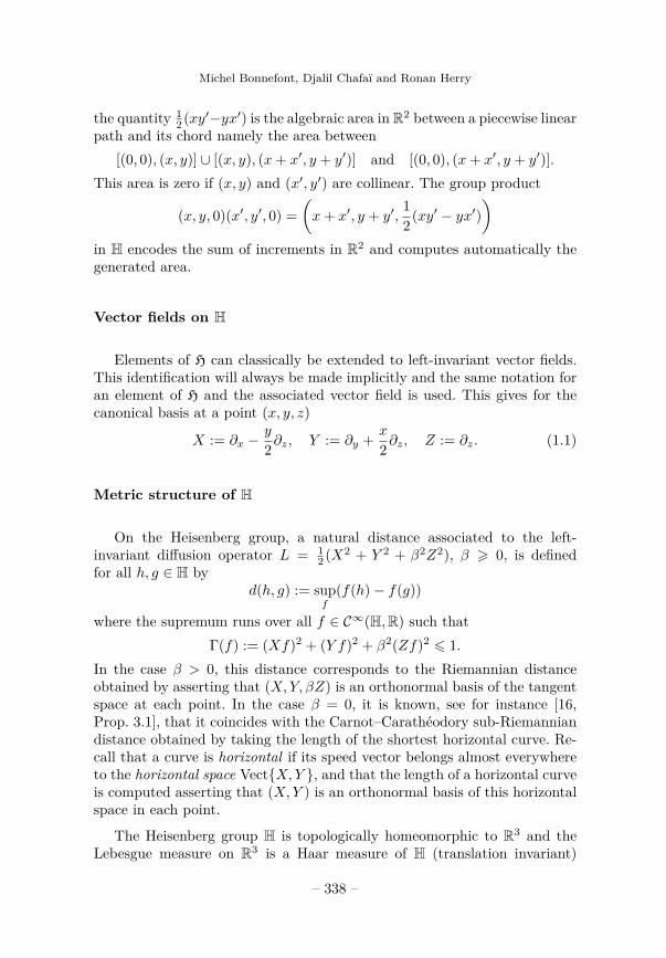
the quantity 12 (xy′−yx′) is the algebraic area in R2 between a piecewise linear
path and its chord namely the area between[(0, 0), (x, y)] ∪ [(x, y), (x+ x′, y + y′)] and [(0, 0), (x+ x′, y + y′)].
This area is zero if (x, y) and (x′, y′) are collinear. The group product
(x, y, 0)(x′, y′, 0) =(x+ x′, y + y′,
12(xy′ − yx′)
)in H encodes the sum of increments in R2 and computes automatically thegenerated area.
Vector fields on H
Elements of H can classically be extended to left-invariant vector fields.This identification will always be made implicitly and the same notation foran element of H and the associated vector field is used. This gives for thecanonical basis at a point (x, y, z)
X := ∂x −y
2∂z, Y := ∂y + x
2∂z, Z := ∂z. (1.1)
Metric structure of H
On the Heisenberg group, a natural distance associated to the left-invariant diffusion operator L = 1
2 (X2 + Y 2 + β2Z2), β > 0, is definedfor all h, g ∈ H by
d(h, g) := supf
(f(h)− f(g))
where the supremum runs over all f ∈ C∞(H,R) such thatΓ(f) := (Xf)2 + (Y f)2 + β2(Zf)2 6 1.
In the case β > 0, this distance corresponds to the Riemannian distanceobtained by asserting that (X,Y, βZ) is an orthonormal basis of the tangentspace at each point. In the case β = 0, it is known, see for instance [16,Prop. 3.1], that it coincides with the Carnot–Carathéodory sub-Riemanniandistance obtained by taking the length of the shortest horizontal curve. Re-call that a curve is horizontal if its speed vector belongs almost everywhereto the horizontal space Vect{X,Y }, and that the length of a horizontal curveis computed asserting that (X,Y ) is an orthonormal basis of this horizontalspace in each point.
The Heisenberg group H is topologically homeomorphic to R3 and theLebesgue measure on R3 is a Haar measure of H (translation invariant)
– 338 –
On logarithmic Sobolev inequalities on the Heisenberg group
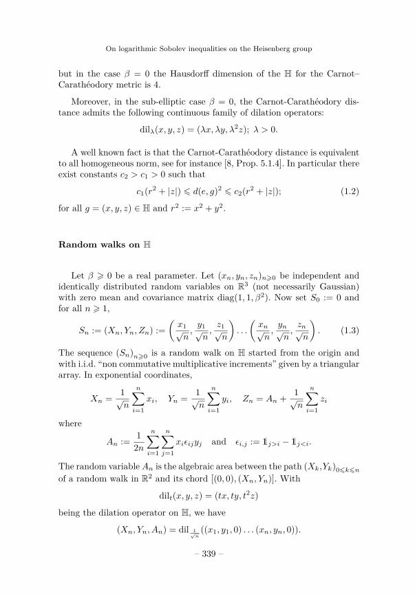
but in the case β = 0 the Hausdorff dimension of the H for the Carnot–Carathéodory metric is 4.
Moreover, in the sub-elliptic case β = 0, the Carnot-Carathéodory dis-tance admits the following continuous family of dilation operators:
dilλ(x, y, z) = (λx, λy, λ2z); λ > 0.
A well known fact is that the Carnot-Carathéodory distance is equivalentto all homogeneous norm, see for instance [8, Prop. 5.1.4]. In particular thereexist constants c2 > c1 > 0 such that
c1(r2 + |z|) 6 d(e, g)2 6 c2(r2 + |z|); (1.2)
for all g = (x, y, z) ∈ H and r2 := x2 + y2.
Random walks on H
Let β > 0 be a real parameter. Let (xn, yn, zn)n>0 be independent andidentically distributed random variables on R3 (not necessarily Gaussian)with zero mean and covariance matrix diag(1, 1, β2). Now set S0 := 0 andfor all n > 1,
Sn := (Xn, Yn, Zn) :=(x1√n,y1√n,z1√n
). . .
(xn√n,yn√n,zn√n
). (1.3)
The sequence (Sn)n>0 is a random walk on H started from the origin andwith i.i.d. “non commutative multiplicative increments” given by a triangulararray. In exponential coordinates,
Xn = 1√n
n∑i=1
xi, Yn = 1√n
n∑i=1
yi, Zn = An + 1√n
n∑i=1
zi
where
An := 12n
n∑i=1
n∑j=1
xiεijyj and εi,j := 1j>i − 1j<i.
The random variableAn is the algebraic area between the path (Xk,Yk)06k6nof a random walk in R2 and its chord [(0, 0), (Xn, Yn)]. With
dilt(x, y, z) = (tx, ty, t2z)
being the dilation operator on H, we have
(Xn, Yn, An) = dil 1√n
((x1, y1, 0) . . . (xn, yn, 0)).
– 339 –
Michel Bonnefont, Djalil Chafaï and Ronan Herry
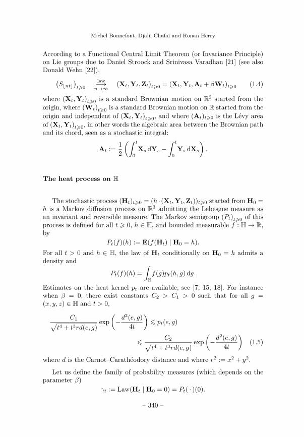
According to a Functional Central Limit Theorem (or Invariance Principle)on Lie groups due to Daniel Stroock and Srinivasa Varadhan [21] (see alsoDonald Wehn [22]),(
Sbntc)t>0
law−→n→∞
(Xt,Yt,Zt)t>0 = (Xt,Yt,At + βWt)t>0 (1.4)
where (Xt,Yt)t>0 is a standard Brownian motion on R2 started from theorigin, where (Wt)t>0 is a standard Brownian motion on R started from theorigin and independent of (Xt,Yt)t>0, and where (At)t>0 is the Lévy areaof (Xt,Yt)t>0, in other words the algebraic area between the Brownian pathand its chord, seen as a stochastic integral:
At := 12
(∫ t
0Xs dYs −
∫ t
0Ys dXs
).
The heat process on H
The stochastic process (Ht)t>0 = (h · (Xt,Yt,Zt))t>0 started from H0 =h is a Markov diffusion process on R3 admitting the Lebesgue measure asan invariant and reversible measure. The Markov semigroup (Pt)t>0 of thisprocess is defined for all t > 0, h ∈ H, and bounded measurable f : H→ R,by
Pt(f)(h) := E(f(Ht) | H0 = h).For all t > 0 and h ∈ H, the law of Ht conditionally on H0 = h admits adensity and
Pt(f)(h) =∫Hf(g)pt(h, g) dg.
Estimates on the heat kernel pt are available, see [7, 15, 18]. For instancewhen β = 0, there exist constants C2 > C1 > 0 such that for all g =(x, y, z) ∈ H and t > 0,
C1√t4 + t3rd(e, g)
exp(−d
2(e, g)4t
)6 pt(e, g)
6C2√
t4 + t3rd(e, g)exp
(−d
2(e, g)4t
)(1.5)
where d is the Carnot–Carathéodory distance and where r2 := x2 + y2.
Let us define the family of probability measures (which depends on theparameter β)
γt := Law(Ht | H0 = 0) = Pt( · )(0).
– 340 –
On logarithmic Sobolev inequalities on the Heisenberg group
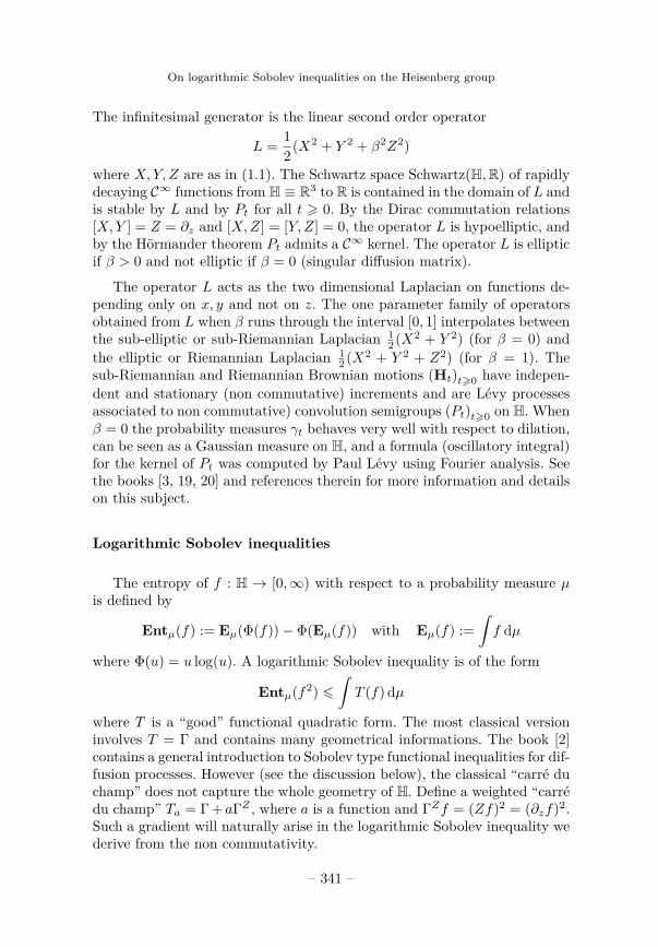
The infinitesimal generator is the linear second order operator
L = 12(X2 + Y 2 + β2Z2)
where X,Y, Z are as in (1.1). The Schwartz space Schwartz(H,R) of rapidlydecaying C∞ functions from H ≡ R3 to R is contained in the domain of L andis stable by L and by Pt for all t > 0. By the Dirac commutation relations[X,Y ] = Z = ∂z and [X,Z] = [Y,Z] = 0, the operator L is hypoelliptic, andby the Hörmander theorem Pt admits a C∞ kernel. The operator L is ellipticif β > 0 and not elliptic if β = 0 (singular diffusion matrix).
The operator L acts as the two dimensional Laplacian on functions de-pending only on x, y and not on z. The one parameter family of operatorsobtained from L when β runs through the interval [0, 1] interpolates betweenthe sub-elliptic or sub-Riemannian Laplacian 1
2 (X2 + Y 2) (for β = 0) andthe elliptic or Riemannian Laplacian 1
2 (X2 + Y 2 + Z2) (for β = 1). Thesub-Riemannian and Riemannian Brownian motions (Ht)t>0 have indepen-dent and stationary (non commutative) increments and are Lévy processesassociated to non commutative) convolution semigroups (Pt)t>0 on H. Whenβ = 0 the probability measures γt behaves very well with respect to dilation,can be seen as a Gaussian measure on H, and a formula (oscillatory integral)for the kernel of Pt was computed by Paul Lévy using Fourier analysis. Seethe books [3, 19, 20] and references therein for more information and detailson this subject.
Logarithmic Sobolev inequalities
The entropy of f : H → [0,∞) with respect to a probability measure µis defined by
Entµ(f) := Eµ(Φ(f))− Φ(Eµ(f)) with Eµ(f) :=∫f dµ
where Φ(u) = u log(u). A logarithmic Sobolev inequality is of the form
Entµ(f2) 6∫T (f) dµ
where T is a “good” functional quadratic form. The most classical versioninvolves T = Γ and contains many geometrical informations. The book [2]contains a general introduction to Sobolev type functional inequalities for dif-fusion processes. However (see the discussion below), the classical “carré duchamp” does not capture the whole geometry of H. Define a weighted “carrédu champ” Ta = Γ +aΓZ , where a is a function and ΓZf = (Zf)2 = (∂zf)2.Such a gradient will naturally arise in the logarithmic Sobolev inequality wederive from the non commutativity.
– 341 –
Michel Bonnefont, Djalil Chafaï and Ronan Herry
Main results
We start with the left-invariant diffusion operator L = 12 (X2+Y 2+β2Z2)
for β > 0 on the Heisenberg group. In the case β > 0, the operator is ellipticand it is not hard to see that a usual logarithmic Sobolev inequality holdsfor its heat kernel. Usual means here that the energy in the right hand side isgiven by the “carré du champ” operator Γ associated to L. Indeed, for β > 0,L can then be thought of as the Laplace–Beltrami operator of a Riemannianmanifold whose Ricci curvature is actually constant and the Bakry–Émerytheory applies. The case β = 0, is much more involved and have attracteda lot of attention. Indeed, the operator L is not anymore elliptic but is stillsub-elliptic. The Ricci curvature tends to −∞ when β goes to 0 and theBakry–Émery theory fails. In this situation, the “carré du champ” operatorcontains only the horizontal part of the gradient. The question whether alogarithmic Sobolev inequality holds was answered positively by Hong-QuanLi in [17] (see (2.2)), see also [1, 10, 14].
In a different direction, even if the classical Bakry–Émery theory fails,Fabrice Baudoin and Nicola Garofalo developed in [6] a generalization ofthe curvature criterion which is well adapted to the sub-Riemannian setting.One can then obtain some (weaker) logarithmic Sobolev inequalities with anelliptic gradient in the energy (see (2.4)).
Our approach is different. We follow the method developed by LeonardGross in [12] for the Gaussian and in [13] for the path space on elliptic Liegroups. It is based on the tensorization property of the logarithmic Sobolevinequality and on the Central Limit Theorem for a random walk. It appliesindifferently both for the sub-elliptic (β = 0) or the elliptic (β > 0) Laplacianon the Heisenberg group. At least when β > 0, our main result Theorem 1.1below is in a way an explicit version of the abstract Theorem 4.1 in [13].
The interest in our result is double: we compute explicitly for the firsttime the gradient that appears in the right hand side of Theorem 4.1 in [13]in the case of the Heisenberg group for all β > 0, and we show, by lookingat the case β = 0, that the method of Gross gives a non degenerate resultfor a sub-Riemannian model. This is surprising and unexpected.
The next theorem, that is the main result of the paper and is provedin Section 3, states the logarithmic Sobolev inequality for γ = γ1. Fromthe scaling property of the heat kernel, we can easily deduce a logarithmicSobolev inequality for γt for every t > 0.
– 342 –
On logarithmic Sobolev inequalities on the Heisenberg group
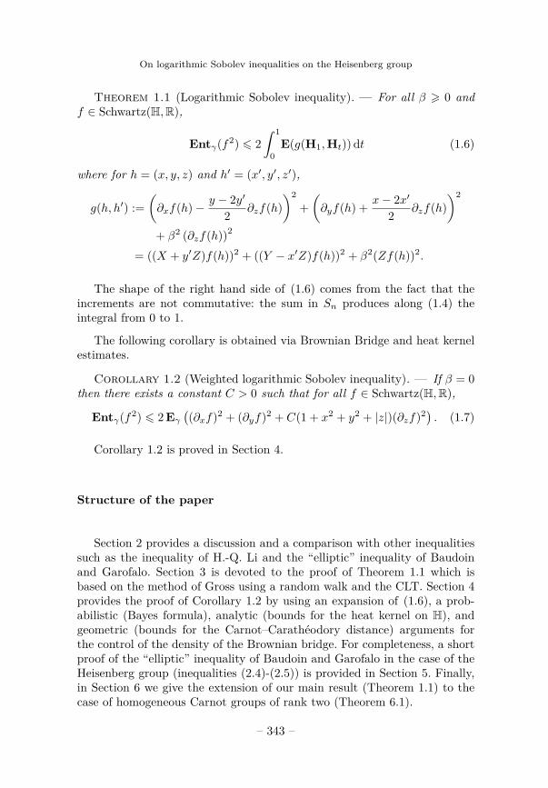
Theorem 1.1 (Logarithmic Sobolev inequality). — For all β > 0 andf ∈ Schwartz(H,R),
The shape of the right hand side of (1.6) comes from the fact that theincrements are not commutative: the sum in Sn produces along (1.4) theintegral from 0 to 1.
The following corollary is obtained via Brownian Bridge and heat kernelestimates.
Corollary 1.2 (Weighted logarithmic Sobolev inequality). — If β = 0then there exists a constant C > 0 such that for all f ∈ Schwartz(H,R),
Section 2 provides a discussion and a comparison with other inequalitiessuch as the inequality of H.-Q. Li and the “elliptic” inequality of Baudoinand Garofalo. Section 3 is devoted to the proof of Theorem 1.1 which isbased on the method of Gross using a random walk and the CLT. Section 4provides the proof of Corollary 1.2 by using an expansion of (1.6), a prob-abilistic (Bayes formula), analytic (bounds for the heat kernel on H), andgeometric (bounds for the Carnot–Carathéodory distance) arguments forthe control of the density of the Brownian bridge. For completeness, a shortproof of the “elliptic” inequality of Baudoin and Garofalo in the case of theHeisenberg group (inequalities (2.4)-(2.5)) is provided in Section 5. Finally,in Section 6 we give the extension of our main result (Theorem 1.1) to thecase of homogeneous Carnot groups of rank two (Theorem 6.1).
– 343 –
Michel Bonnefont, Djalil Chafaï and Ronan Herry
2. Discussion and comparison with other inequalities
Novelty
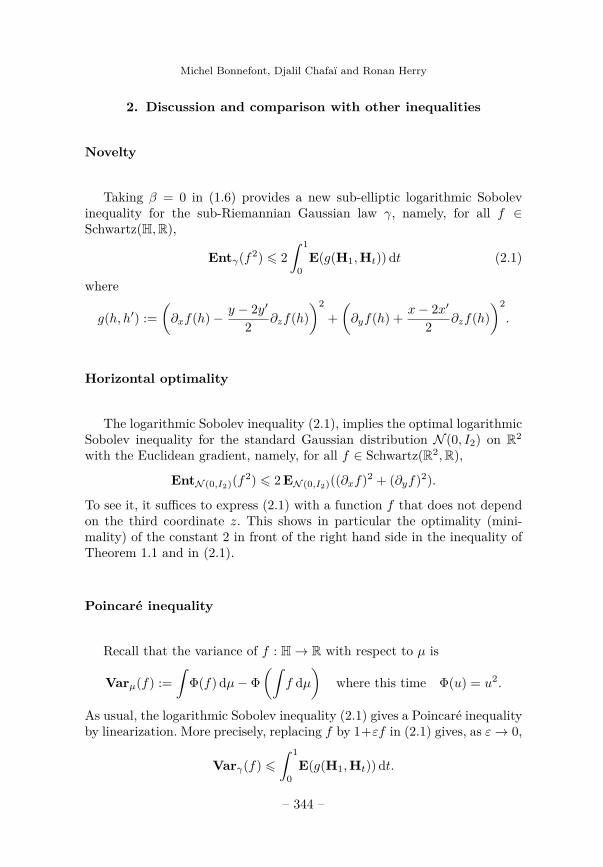
Taking β = 0 in (1.6) provides a new sub-elliptic logarithmic Sobolevinequality for the sub-Riemannian Gaussian law γ, namely, for all f ∈Schwartz(H,R),
Entγ(f2) 6 2∫ 1
0E(g(H1,Ht)) dt (2.1)
where
g(h, h′) :=(∂xf(h)− y − 2y′
2 ∂zf(h))2
+(∂yf(h) + x− 2x′
2 ∂zf(h))2.
Horizontal optimality
The logarithmic Sobolev inequality (2.1), implies the optimal logarithmicSobolev inequality for the standard Gaussian distribution N (0, I2) on R2
with the Euclidean gradient, namely, for all f ∈ Schwartz(R2,R),
EntN (0,I2)(f2) 6 2 EN (0,I2)((∂xf)2 + (∂yf)2).
To see it, it suffices to express (2.1) with a function f that does not dependon the third coordinate z. This shows in particular the optimality (mini-mality) of the constant 2 in front of the right hand side in the inequality ofTheorem 1.1 and in (2.1).
Poincaré inequality
Recall that the variance of f : H→ R with respect to µ is
Varµ(f) :=∫
Φ(f) dµ− Φ(∫
f dµ)
where this time Φ(u) = u2.
As usual, the logarithmic Sobolev inequality (2.1) gives a Poincaré inequalityby linearization. More precisely, replacing f by 1+εf in (2.1) gives, as ε→ 0,
Varγ(f) 6∫ 1
0E(g(H1,Ht)) dt.
– 344 –
On logarithmic Sobolev inequalities on the Heisenberg group
Comparison with H.-Q. Li inequality
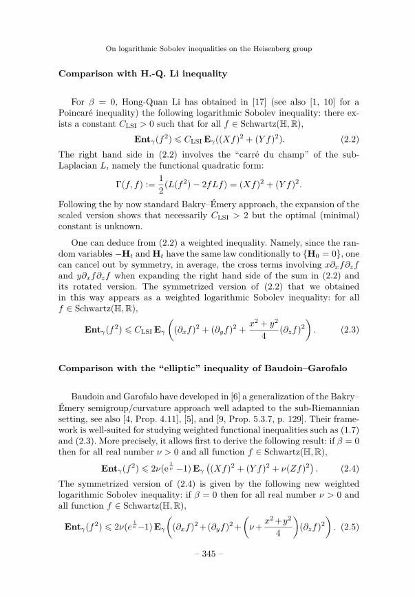
For β = 0, Hong-Quan Li has obtained in [17] (see also [1, 10] for aPoincaré inequality) the following logarithmic Sobolev inequality: there ex-ists a constant CLSI > 0 such that for all f ∈ Schwartz(H,R),
Entγ(f2) 6 CLSI Eγ((Xf)2 + (Y f)2). (2.2)The right hand side in (2.2) involves the “carré du champ” of the sub-Laplacian L, namely the functional quadratic form:
Γ(f, f) := 12(L(f2)− 2fLf) = (Xf)2 + (Y f)2.
Following the by now standard Bakry–Émery approach, the expansion of thescaled version shows that necessarily CLSI > 2 but the optimal (minimal)constant is unknown.
One can deduce from (2.2) a weighted inequality. Namely, since the ran-dom variables −Ht and Ht have the same law conditionally to {H0 = 0}, onecan cancel out by symmetry, in average, the cross terms involving x∂xf∂zfand y∂xf∂zf when expanding the right hand side of the sum in (2.2) andits rotated version. The symmetrized version of (2.2) that we obtainedin this way appears as a weighted logarithmic Sobolev inequality: for allf ∈ Schwartz(H,R),
Entγ(f2) 6 CLSI Eγ
((∂xf)2 + (∂yf)2 + x2 + y2
4 (∂zf)2). (2.3)
Comparison with the “elliptic” inequality of Baudoin–Garofalo
Baudoin and Garofalo have developed in [6] a generalization of the Bakry–Émery semigroup/curvature approach well adapted to the sub-Riemanniansetting, see also [4, Prop. 4.11], [5], and [9, Prop. 5.3.7, p. 129]. Their frame-work is well-suited for studying weighted functional inequalities such as (1.7)and (2.3). More precisely, it allows first to derive the following result: if β = 0then for all real number ν > 0 and all function f ∈ Schwartz(H,R),
Entγ(f2) 6 2ν(e 1ν −1) Eγ
((Xf)2 + (Y f)2 + ν(Zf)2) . (2.4)
The symmetrized version of (2.4) is given by the following new weightedlogarithmic Sobolev inequality: if β = 0 then for all real number ν > 0 andall function f ∈ Schwartz(H,R),
Entγ(f2) 6 2ν(e 1ν−1) Eγ
((∂xf)2 +(∂yf)2 +
(ν+ x2 +y2
4
)(∂zf)2
). (2.5)
– 345 –
Michel Bonnefont, Djalil Chafaï and Ronan Herry
Our weighted inequality (1.7) is close to the weighted inequalities (2.3)and (2.5).
For the reader convenience, we provide a short proof of (2.4) and (2.5)in Section 5. This proof is the Heisenberg group specialization of the proofgiven in [9, Prop. 5.3.7, p. 129] (PhD thesis of the first author) see also [4,Prop. 4.11] (PhD advisor of the first author).
Extensions and open questions.
The Heisenberg group is the simplest non-trivial example of a Carnotgroup in other words stratified nilpotent Lie group. Those groups have astrong geometric meaning both in standard and stochastic analysis, see forinstance [3] for the latter point. Theorem 1.1 is extended to homogeneousCarnot group of rank two in Section 6. Note that the criterion of Baudoin andGarofalo [6] holds for Carnot groups of rank two and an inequality similarto (2.4) holds in this context, see [4].
The bounds on the distance and the heat kernel used to derive theweighted inequality (1.7) are not available for general Carnot groups andit should require more work to obtain an equivalent of Corollary 1.2. As acomparison, note that a version of (2.2) exists on groups with a so calledH-structure, see [11], but a general version on Carnot groups is unknowndue to the lack of general estimates for the heat kernel. An extension ofTheorem 1.1 in the case of higher dimensional Carnot groups or in the caseof curved sub-Riemannian space as CR spheres or anti-de Sitter spaces isopened.
Moreover, in the context and spirit of the work of Leonard Gross [13] inthe elliptic case, an approach at the level of paths space should be available.It is also natural to ask about a direct analytic proof or semigroup proof ofthe inequality of Theorem 1.1, without using the Central Limit Theorem.
3. Proof of Theorem 1.1
Fix a real β > 0. Consider (xn, yn, zn)n>1 a sequence of independent andidentically distributed random variables with Gaussian law of mean zero andcovariance matrix diag(1, 1, β2). Let Sn be as in (1.3). The Central LimitTheorem gives
Snlaw−→n→∞
γ.
– 346 –
On logarithmic Sobolev inequalities on the Heisenberg group
The law νn of Sn satisfies νn = (µn)∗n where the convolution takes placein H and where µn is the Gaussian law on R3 with covariance matrixdiag(1/n, 1/n, β2/n).
For all i = 1, . . . , n, let us define
Sn,i := (Xn, Yn, Zn, Xn,i, Yn,i)
where
Xn,i := − 1√n
n∑j=1
εijxj and Yn,i := − 1√n
n∑j=1
εijyj .
The optimal logarithmic Sobolev inequality for the standard Gaussian mea-sure N (0, I3n) on R3n gives, for all g ∈ Schwartz(R3n,R),
EntN (0,I3n)(g2) 6 2 EN (0,I3n)
(n∑i=1
(∂xig)2 + (∂yig)2 + (∂zig)2
).
Let sn : R3n → H be the map such that Sn = sn((x1, y1, z1), . . . , (xn, yn, zn)).For some f ∈ Schwartz(H,R) the function g = f(sn) satisfies
∂xig(sn) = 1√n
(∂xf −
Yn,i2 ∂zf
)(sn),
∂yig(sn) = 1√n
(∂yf + Xn,i
2 ∂zf
)(sn),
∂zig(sn) = β√n
(∂zf)(sn).
It follows that for all f ∈ Schwartz(H,R), denoting νn := Law(Sn),
Entνn(f2) 6 2n
n∑i=1
E(h(Sn,i)) = 2 E(
1n
n∑i=1
h(Sn,i))
(3.1)
where h : R5 → R is defined from f by
h(x, y, z, x′, y′) :=((
∂x −y′
2 ∂z)f(x, y, z)
)2
+((
∂y + x′
2 ∂z)f(x, y, z)
)2+ β2(∂zf(x, y, z))2
The right hand side of (3.1) as n→∞ is handled by explaining the law of Sn,ithrough a triangular array of increments of the process we anticipated in thelimit. More precisely, let ((Xt,Yt))t>0 be a standard Brownian motion onR2 started from the origin, let (At)t>0 be its Lévy area, and let (Wt)t>0 be a
– 347 –
Michel Bonnefont, Djalil Chafaï and Ronan Herry
Brownian motion on R starting from the origin, independent of (Xt,Yt)t>0.Let us define, for n > 1 and 1 6 i 6 n,
ξn,i :=√n(
X in−X i−1
n
),
ηn,i :=√n(
Y in−Y i−1
n
),
ζn,i :=√n(
W in−W i−1
n
).
For all fixed n > 1, the random variables (ξn,i)16i6n, (ηn,i)16i6n, and(ζn,i)16i6n are independent and identically distributed with Gaussian lawN (0, 1). Let us define now
Xn := 1√n
n∑i=1
ξn,i, Yn := 1√n
n∑i=1
ηn,i,
An := 12n
n∑i=1
n∑j=1
ξn,iεi,jηn,i, Zn := β1√n
n∑i=1
ζn,i +An,
Xn,i := − 1√n
n∑j=1
εi,jξn,j , Yn,i := − 1√n
n∑j=1
εi,jηn,i.
We have then the equality in distribution
(Xn, Yn, Zn −An, Xn,i, Yn,i)d=(
X1,Y1, βW1,X1 −(
X i−1n
+ X in
),Y1 −
(Y i−1
n+ Y i
n
)).
Moreover, as i/n→ s ∈ [0, 1], we have the convergence in distribution
Sn,i := (Xn, Yn, Zn, Xn,i, Yn,i)d−→
n→∞(X1,Y1,A1 + βW1,X1 − 2Xs,Y1 − 2Ys).
It follows that for all continuous and bounded h : R5 → R,
1n
n∑i=1
E(h(Sn,i)) =∫ 1
0E(h(Xn, Yn, Zn, Xn,
btncn
, Yn,btncn
)dt
−→n→∞
∫ 1
0E(h(X1,Y1,A1 + βW1,X1 − 2Xt,Y1 − 2Yt)) dt.
4. Proof of Corollary 1.2
Let us consider (1.6) with β = 0. By expanding the right-hand side, andusing the fact that the conditional law of H1 given {H0 = 0} is invariant
– 348 –
On logarithmic Sobolev inequalities on the Heisenberg group
by central symmetry, we get a symmetrized weighted logarithmic Sobolevinequality: for all f ∈ Schwartz(H,R),Entγ(f2) 6 2 E
((∂xf)2(H1) + (∂yf)2(H1)
)+ 1
2
∫ 1
0E(E((X1 − 2Xt)2 + (Y1 − 2Yt)2 ∣∣H1
)(∂zf)2(H1)
)dt
6 2 E((∂xf)2(H1) + (∂yf)2(H1)
)+ E
((X2
1 + Y21)(∂zf)2(H1)
)+ 4 E
((∂zf)2(H1)
∫ 1
0E(X2t + Y2
t | H1)
dt).
The desired result is a direct consequence of the following lemma.
Lemma 4.1 (Bridge control). — There exists a constant C > 0 such thatfor all 0 6 t 6 1 and h = (x, y, z) ∈ H,
E(X2t + Y2
t | H1 = h) 6 C(t2d2(e, h) + t)and ∫ 1
0E(X2
t + Y2t | H1 = h) dt 6 C(1 + x2 + y2 + |z|).
Note that for the classical euclidean Brownian motionE(‖Bt‖2 | B1) = t2‖B1‖2 + nt(1− t).
Proof of Lemma 4.1. — For all random variables U, V , we denote by ϕUthe density of U and by ϕU |V=v the conditional density of U given {V = v}.For all 0 < t 6 1 and k ∈ H,
E(X2t + Y2
t | H1 = k) =∫Hr2g ϕHt|H1=k(g) dg
where r2g = x2
g + y2g and g = (xg, yg, zg). Recall that pt(h, g) := ϕHt=g|H0=h
and that e := (0, 0, 0) is the origin in H. Thanks to the Bayes formula, forall g, k ∈ H,
ϕHt|H1=k(g) =ϕ(Ht,H1)(g, k)
ϕH1(k) =ϕHt
(g)ϕH1|Ht=g(k)ϕH1(k) = pt(e, g)p1−t(g, k)
p1(e, k) .
Back to our objective, we have
E(X2t + Y2
t | H1 = k) =
∫pt(e, g) r2
g p1−t(g, k) dg
p1(e, k)
6
∫pt(e, g)d2(e, g)p1−t(g, k) dg
p1(e, k) .
– 349 –
Michel Bonnefont, Djalil Chafaï and Ronan Herry
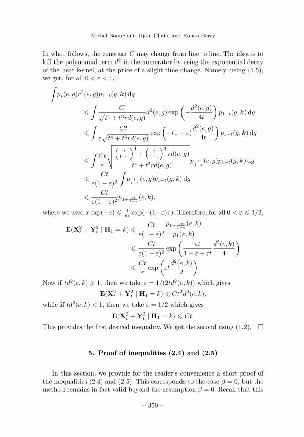
In what follows, the constant C may change from line to line. The idea is tokill the polynomial term d2 in the numerator by using the exponential decayof the heat kernel, at the price of a slight time change. Namely, using (1.5),we get, for all 0 < ε < 1,∫
pt(e, g)r2(e, g)p1−t(g, k) dg
6∫
C√t4 + t3rd(e, g)
d2(e, g) exp(−d
2(e, g)4t
)p1−t(g, k) dg
6∫
Ct
ε√t4 + t3rd(e, g)
exp(−(1− ε)d
2(e, g)4t
)p1−t(g, k) dg
6∫Ct
ε
√√√√( t1−ε
)4+(
t1−ε
)3rd(e, g)
t4 + t3rd(e, g) p t1−ε
(e, g)p1−t(g, k) dg
6Ct
ε(1− ε)2
∫p t
1−ε(e, g)p1−t(g, k) dg
6Ct
ε(1− ε)2 p1+ εt1−ε
(e, k),
where we used x exp(−x) 6 1eε exp(−(1−ε)x). Therefore, for all 0 < ε 6 1/2,
E(X2t + Y2
t | H1 = k) 6 Ct
ε(1− ε)2
p1+ εt1−ε
(e, k)p1(e, k)
6Ct
ε(1− ε)2 exp(
εt
1− ε+ εt
d2(e, k)4
)6Ct
εexp
(εtd2(e, k)
2
).
Now if td2(e, k) > 1, then we take ε = 1/(2td2(e, k)) which givesE(X2
t + Y2t | H1 = k) 6 Ct2d2(e, k),
while if td2(e, k) < 1, then we take ε = 1/2 which givesE(X2
t + Y2t | H1 = k) 6 Ct.
This provides the first desired inequality. We get the second using (1.2). �
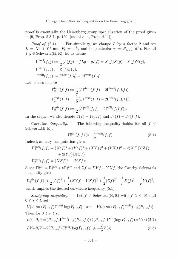
5. Proof of inequalities (2.4) and (2.5)
In this section, we provide for the reader’s convenience a short proof ofthe inequalities (2.4) and (2.5). This corresponds to the case β = 0, but themethod remains in fact valid beyond the assumption β = 0. Recall that this
– 350 –
On logarithmic Sobolev inequalities on the Heisenberg group
proof is essentially the Heisenberg group specialization of the proof givenin [9, Prop. 5.3.7, p. 129] (see also [4, Prop. 4.11]).
Proof of (2.4). — For simplicity, we change L by a factor 2 and setL = X2 + Y 2 and Pt = etL, and in particular γ = P1/2( · )(0). For allf, g ∈ Schwartz(H,R), let us define
2 + νΓvert2 and Zf = XY f − Y Xf , the Cauchy–Schwarz’s
inequality gives
Γmix2 (f, f) > 1
2(Lf)2 + 12(XY f + Y Xf)2 + 1
2(Zf)2 − 1νX(f)2 − 1
νY (f)2,
which implies the desired curvature inequality (5.1).
Semigroup inequality. — Let f ∈ Schwartz(H,R) with f > 0. For all0 6 s 6 t, setU(s) := (Pt−sf) Γhori log(Pt−sf) and V (s) := (Pt−sf) Γelli(log(Pt−sf)).Then for 0 6 s 6 t,LU+∂sU=(Pt−sf)Γhori(log(Pt−sf))6(Pt−sf)Γelli(log(Pt−sf))=V (s) (5.2)
LV+∂sV =2(Pt−sf) Γmix2 (log(Pt−sf)) > −2
νV (s). (5.3)
– 351 –
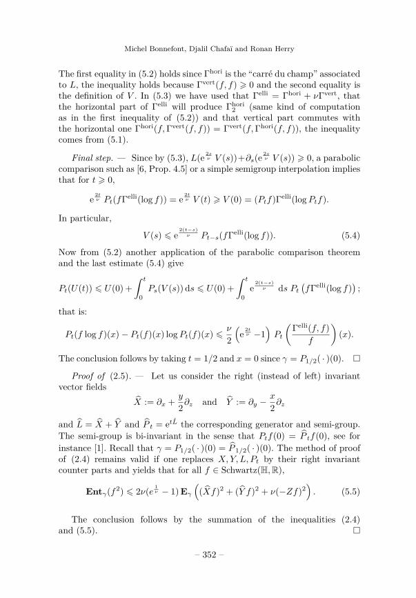
Michel Bonnefont, Djalil Chafaï and Ronan Herry
The first equality in (5.2) holds since Γhori is the “carré du champ” associatedto L, the inequality holds because Γvert(f, f) > 0 and the second equality isthe definition of V . In (5.3) we have used that Γelli = Γhori + νΓvert, thatthe horizontal part of Γelli will produce Γhori
2 (same kind of computationas in the first inequality of (5.2)) and that vertical part commutes withthe horizontal one Γhori(f,Γvert(f, f)) = Γvert(f,Γhori(f, f)), the inequalitycomes from (5.1).
Final step. — Since by (5.3), L(e 2sν V (s))+∂s(e
2sν V (s)) > 0, a parabolic
comparison such as [6, Prop. 4.5] or a simple semigroup interpolation impliesthat for t > 0,
e 2tν Pt(fΓelli(log f)) = e 2t
ν V (t) > V (0) = (Ptf)Γelli(logPtf).
In particular,
V (s) 6 e2(t−s)ν Pt−s(fΓelli(log f)). (5.4)
Now from (5.2) another application of the parabolic comparison theoremand the last estimate (5.4) give
Pt(U(t)) 6 U(0) +∫ t
0Ps(V (s)) ds 6 U(0) +
∫ t
0e
2(t−s)ν ds Pt
(fΓelli(log f)
);
that is:
Pt(f log f)(x)− Pt(f)(x) logPt(f)(x) 6 ν
2
(e 2tν −1
)Pt
(Γelli(f, f)
f
)(x).
The conclusion follows by taking t = 1/2 and x = 0 since γ = P1/2( · )(0). �
Proof of (2.5). — Let us consider the right (instead of left) invariantvector fields
X := ∂x + y
2∂z and Y := ∂y −x
2∂z
and L = X + Y and P t = etL the corresponding generator and semi-group.The semi-group is bi-invariant in the sense that Ptf(0) = P tf(0), see forinstance [1]. Recall that γ = P1/2( · )(0) = P 1/2( · )(0). The method of proofof (2.4) remains valid if one replaces X,Y, L, Pt by their right invariantcounter parts and yields that for all f ∈ Schwartz(H,R),
Entγ(f2) 6 2ν(e 1ν − 1) Eγ
((Xf)2 + (Y f)2 + ν(−Zf)2
). (5.5)
The conclusion follows by the summation of the inequalities (2.4)and (5.5). �
– 352 –
On logarithmic Sobolev inequalities on the Heisenberg group
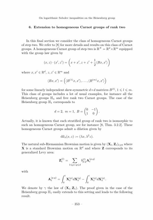
6. Extension to homogeneous Carnot groups of rank two
In this final section we consider the class of homogeneous Carnot groupsof step two. We refer to [8] for more details and results on this class of Carnotgroups. A homogeneous Carnot group of step two is RN = Rd×Rm equippedwith the group law given by
(x, z) · (x′, z′) =(x+ x′, z + z′ + 1
2 〈Bx, x′〉)
where x, x′ ∈ Rd, z, z′ ∈ Rm and
〈Bx, x′〉 =(〈B(1)x, x′〉, . . . , 〈B(m)x, x′〉
)for some linearly independent skew-symmetric d×dmatrices B(l), 1 6 l 6 m.This class of groups includes a lot of usual examples, for instance all theHeisenberg groups Hn and free rank two Carnot groups. The case of theHeisenberg group H1 corresponds to
d = 2, m = 1, B =(
0 −11 0
).
Actually, it is known that each stratified group of rank two is isomorphic tosuch an homogeneous Carnot group, see for instance [8, Thm. 3.2.2]. Thesehomogeneous Carnot groups admit a dilation given by
dilλ(x, z) := (λx, λ2z).
The natural sub-Riemannian Brownian motion is given by (Xt,Zt)t>0 whereX is a standard Brownian motion on Rd and where Z corresponds to itsgeneralized Levy area:
Z(l)t =
∑16p<q6d
b(l)p,qA
(p,q)t
with
A(p,q)t =
∫ t
0X(p)s dX(q)
s −∫ t
0X(q)s dX(p)
s .
We denote by γ the law of (X1,Z1). The proof given in the case of theHeisenberg group H1 easily extends to this setting and leads to the followingresult.
– 353 –
Michel Bonnefont, Djalil Chafaï and Ronan Herry
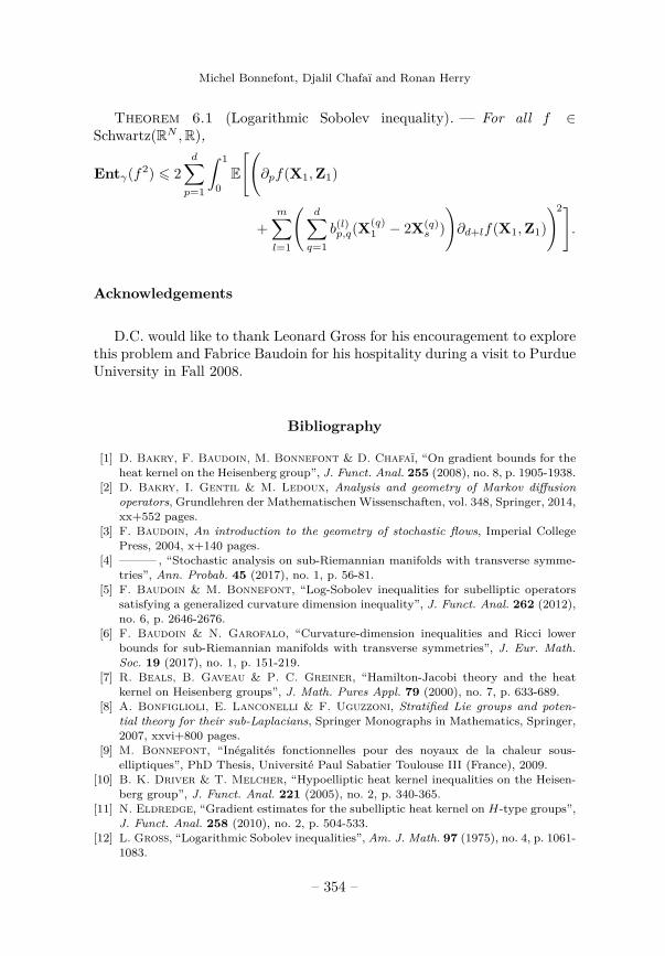
Theorem 6.1 (Logarithmic Sobolev inequality). — For all f ∈Schwartz(RN ,R),
Entγ(f2) 6 2d∑p=1
∫ 1
0E
[(∂pf(X1,Z1)
+m∑l=1
(d∑q=1
b(l)p,q(X
(q)1 − 2X(q)
s ))∂d+lf(X1,Z1)
)2].
Acknowledgements
D.C. would like to thank Leonard Gross for his encouragement to explorethis problem and Fabrice Baudoin for his hospitality during a visit to PurdueUniversity in Fall 2008.
Bibliography
[1] D. Bakry, F. Baudoin, M. Bonnefont & D. Chafaï, “On gradient bounds for theheat kernel on the Heisenberg group”, J. Funct. Anal. 255 (2008), no. 8, p. 1905-1938.
[2] D. Bakry, I. Gentil & M. Ledoux, Analysis and geometry of Markov diffusionoperators, Grundlehren der Mathematischen Wissenschaften, vol. 348, Springer, 2014,xx+552 pages.
[3] F. Baudoin, An introduction to the geometry of stochastic flows, Imperial CollegePress, 2004, x+140 pages.
[4] ———, “Stochastic analysis on sub-Riemannian manifolds with transverse symme-tries”, Ann. Probab. 45 (2017), no. 1, p. 56-81.
[5] F. Baudoin & M. Bonnefont, “Log-Sobolev inequalities for subelliptic operatorssatisfying a generalized curvature dimension inequality”, J. Funct. Anal. 262 (2012),no. 6, p. 2646-2676.
[6] F. Baudoin & N. Garofalo, “Curvature-dimension inequalities and Ricci lowerbounds for sub-Riemannian manifolds with transverse symmetries”, J. Eur. Math.Soc. 19 (2017), no. 1, p. 151-219.
[7] R. Beals, B. Gaveau & P. C. Greiner, “Hamilton-Jacobi theory and the heatkernel on Heisenberg groups”, J. Math. Pures Appl. 79 (2000), no. 7, p. 633-689.
[8] A. Bonfiglioli, E. Lanconelli & F. Uguzzoni, Stratified Lie groups and poten-tial theory for their sub-Laplacians, Springer Monographs in Mathematics, Springer,2007, xxvi+800 pages.
[9] M. Bonnefont, “Inégalités fonctionnelles pour des noyaux de la chaleur sous-elliptiques”, PhD Thesis, Université Paul Sabatier Toulouse III (France), 2009.
[10] B. K. Driver & T. Melcher, “Hypoelliptic heat kernel inequalities on the Heisen-berg group”, J. Funct. Anal. 221 (2005), no. 2, p. 340-365.
[11] N. Eldredge, “Gradient estimates for the subelliptic heat kernel on H-type groups”,J. Funct. Anal. 258 (2010), no. 2, p. 504-533.
[12] L. Gross, “Logarithmic Sobolev inequalities”, Am. J. Math. 97 (1975), no. 4, p. 1061-1083.
– 354 –
On logarithmic Sobolev inequalities on the Heisenberg group
[13] ———, “Logarithmic Sobolev inequalities on Lie groups”, Ill. J. Math. 36 (1992),no. 3, p. 447-490.
[14] W. Hebisch & B. Zegarliński, “Coercive inequalities on metric measure spaces”,J. Funct. Anal. 258 (2010), no. 3, p. 814-851.
[15] H. Hueber & D. Müller, “Asymptotics for some Green kernels on the Heisenberggroup and the Martin boundary”, Math. Ann. 283 (1989), no. 1, p. 97-119.
[16] D. Jerison & A. Sánchez-Calle, “Subelliptic, second order differential operators”,in Complex analysis, III (College Park, Md., 1985–86), Lecture Notes in Mathemat-ics, vol. 1277, Springer, 1987, p. 46-77.
[17] H.-Q. Li, “Estimation optimale du gradient du semi-groupe de la chaleur sur le groupede Heisenberg”, J. Funct. Anal. 236 (2006), no. 2, p. 369-394.
[18] ———, “Estimations optimales du noyau de la chaleur sur les groupes de type Heisen-berg”, J. Reine Angew. Math. 646 (2010), p. 195-233.
[19] R. Montgomery, A tour of subriemannian geometries, their geodesics and appli-cations, Mathematical Surveys and Monographs, vol. 91, American MathematicalSociety, 2002, xx+259 pages.
[20] D. Neuenschwander, Probabilities on the Heisenberg group. Limit theoremsand Brownian motion, Lecture Notes in Mathematics, vol. 1630, Springer, 1996,viii+139 pages.
[21] D. W. Stroock & S. R. S. Varadhan, “Limit theorems for random walks on Liegroups”, Sankhya, Ser. A 35 (1973), no. 3, p. 277-294.
[22] D. Wehn, “Probabilities on Lie groups”, Proc. Natl. Acad. Sci. USA 48 (1962),p. 791-795.