On Maximum Differential Graph Coloring

Yifan Hu1, Stephen Kobourov2, and Sankar Veeramoni2

1 AT&T Labs Research, Florham Park, NJ, USAyifanhu@research.att.com

2 Computer Science Dept., University of Arizona, Tucson, AZ, USA{kobourov,sankar}@cs.arizona.edu

Abstract. We study the maximum differential graph coloring problem,in which the goal is to find a vertex labeling for a given undirected graphthat maximizes the label difference along the edges. This problem has itsorigin in map coloring, where not all countries are necessarily contiguous.We define the differential chromatic number and establish the equivalenceof the maximum differential coloring problem to that of k-Hamiltonianpath. As computing the maximum differential coloring is NP-Complete,we describe an exact backtracking algorithm and a spectral-based heuris-tic. We also discuss lower bounds and upper bounds for the differentialchromatic number for several classes of graphs.

1 Introduction

The Four Color Theorem states that only four colors are needed to color anymap so that no neighboring countries share the same color. This theorem assumesthat each country forms a contiguous region in the map. However, if countriesin the map are not all contiguous then the result no longer holds [6]. Instead,this necessitates use of a unique color for each country to avoid ambiguity. As aresult, the number of colors needed is equal to the number of countries.

Given a map, we define the country graph G = {V,E} to be the undirectedgraph where countries are nodes and two countries are connected by an edgeif they share a nontrivial boundary. We then consider the problem of assigningcolors to nodes of G so that the color distance between nodes that share an edgeis maximized. Figure 1 gives an illustration of this map coloring problem.

As not all colors make suitable choices for country colors, a good color paletteis often a gradation of certain “map-like colors”. Furthermore, if the final resultis to be printed in black and white, then the color space is strictly 1D. Wetherefore make the assumption that the colors form a line in the color space,and model our map coloring problem as one of node labeling of the graph, wherethe available labels are from set C = {all permutations of {1, 2, · · · |V |}}. Thisbrings us to the maximum differential graph coloring problem, in which we aimto find a vertex labeling for a given undirected graph that maximizes the labeldifference along the edges in the graph.

More formally, we are looking for a labeling function, a bijection c : V →{1, 2, . . . , |V |}, that solves the following MaxMin optimization problem:

maxc∈C

min{i,j}∈E

wij |c(i)− c(j)| (1)

Here wij are positive weights representing importance of keeping the difference oflabels between nodes i and j large. To simplify the problem further, throughoutthis paper we assume wij = 1.

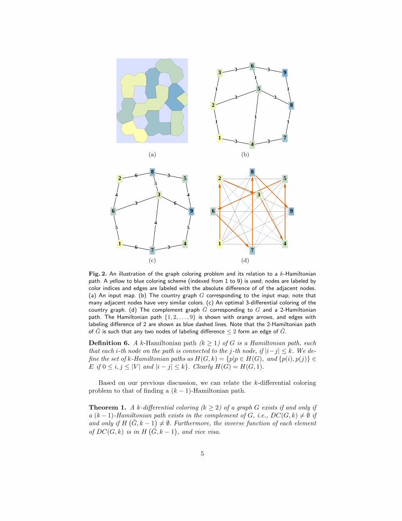
Figure 2 illustrates the graph coloring problem. We use a color palette of yel-low to blue, indexed from 1 to 9. Figure 2(a) shows a map with 9 countries, withone non-contiguous country (its two components are at the center, and to the farright of the map). Figure 2(b) shows the corresponding country graph. The nodelabeling is not optimal, with many adjacent nodes having label difference of 1.Figure 2(c) gives the optimal node labeling, with a minimal label difference of 3.The map in Figure 2(a) is in fact colored using this optimal coloring scheme,which gives distinctive colors for neighboring countries.

In this paper we define the differential chromatic number and show a cor-respondence between the maximum differential graph coloring problem and theHamiltonian path problem in the complement graph. We also provide exact andheuristic algorithms for computing good solutions. In Section 3 we establish therelationship between this problem and that of finding a k-Hamiltonian path. aheuristic algorithm on a number of well known graphs. Section 5 gives resultsfor some special graphs. We conclude the paper with Section 6.

2 Related Work

The problem of maximum differential coloring of graphs arises in the contextof coloring a map in which not all regions are necessarily contiguous [6, 7]. Avariation of the differential graph coloring problem was studied by Dillencourtet al. [4], under the assumption that all colors in the color spectrum are available.This makes the problem continuous rather than discrete. A heuristic algorithmbased on the force-directed model is used to select |V | colors as far apart aspossible in the 3-dimensional color space. However this algorithm cannot be useddirectly for the general map coloring problem, as maps are typically colored with“map-like colors”, often light, pastel colors which come from a very restrictedsubset of the color spectrum. It may be possible to adapt the algorithm and applyit to a lower-dimensional color manifold, but because the algorithm is greedy itis more likely to converge to local minimum in lower dimensional space.

The problem of finding a permutation that minimizes the labeling differencesalong the edges is well-studied problem in the context of minimum bandwidthor wavefront reduction ordering for sparse matrices. It is known that the band-width problem is NP-complete, with a reduction from 3SAT dating to 1975 [11].Moreover, it is NP-complete to find any constant approximation, even when re-stricting the problem to trees [1, 15]. A number of effective heuristics for thatproblem have been proposed [8, 9, 13].

The complement of the bandwidth problem is that of maximizing the labelingdifference along the edges and is less well known as the antibandwidth problem.

2

Tamassia

TollisBattista

Goodrich

LiottaBridgeman

Fanto

Garg

Vismara

Brandes

Wagner

Eades

Didimo

Gelfand

Vargiu

TassinariParise

Kosaraju

Shubina

Chan

Dogrusoz

Madden

Castello

Mili

Biedl

Kakoulis

Six

Xia

Papakostas

Whitesides

Bose

Demetrescu

Finocchi

Patrignani

PizzoniaLenhart

Lubiw

Bertolazzi

Buti

Carmignani

MateraMarcandalli

Lillo

Vernacotola

Barbagallo

Boyer

Cortese

Mariani

Eppstein

Cheng

Duncan

Gajer

Tanenbaum

Scheinerman

Wagner

DickersonMeng

Wismath

ElGindy

Meijer

Dujmovic

Fellows

Hallett

Kitching

McCartin

Nishimura

Ragde

RosamondSuderman Giacomo

Felsner

Binucci

NonatoCruz

Rusu

Chanda

SchreiberHimsolt

Raitner

Marshall

Kaufmann

Cornelsen

Kenis

Dwyer

Kopf

Herman

BaurBenkert

Gaertler Lerner

EiglspergerSchank

Kuchem

Houle

QuigleyLee

Lin LinCohen

Huang Feng

WebberRuskey

Garvan

Friedrich

Nascimento

Murray

Leonforte

Pop

Madden

Genc

Kikusts

Freivalds

Himsholt

Frick

Bertault

Feng

Fosmeier

Grigorescu

Powers

Shermer

Ryall

Thiele

JohansenBretscher

Brandenburg

Marks

MutzelJunger

Kobourov

Bachl

Edachery

Sen

Forster

Rohrer

Pick

Bachmaier

Lesh

AndalmanRuml

Shieber

Kruja

Blair

Waters

Leipert

Lee

Odenthal

Gutwenger

Buchheim

Ziegler

Klau

Klein Barth

Kupke

Weiskircher

Percan

Hundack

Pouchkarev

Thome

Brockenauer

Fialko

KrugerNaher

Alberts

AmbrasKoch

Efrat

Wenk

Erten

Harding

Wampler

Yee

Pitta

Le

Navabi

Roxborough

Trumbach

SkodinisHirschberg

North

Dobkin

Gansner

Koutsofios

Ellson

Woodhull

SymvonisWood

Alt

GodauFekete

Dean

Hutchinson

Ramos

McAllister

Snoeyink

Gomez

Toussaint

Italiano

Iturriaga

Morin

Closson

Gartshore

Dyck

JoevenazzoNickle

Wilsdon

Fernau

Vince

Lynn

Rucevskis

Brus

Keskin

Vogelmann

Ludwig

Mehldau

Miller

Hes

Kant

SteckelbachBubeck

Ritt

Rosenstiel

Chrobak Nakano

Nishizeki

TokuyamaWatanabe

Miura

Yoshikawa

Rahman

Uno

Miyazawa

Ghosh

Naznin

Egi

Asano

Hurtado

Sablowski

Jourdan

Rival Zaguia

Hashemi

Kisielewicz

Alzohairi

Barouni

Jaoua

Chen

Lu

YenLiao

Chuang

Lin

Lambe

Twarog

Lozada

Neto

Rosi

Stolfi

Eckersley

MelanconRuiter

Delest

Shahrokhi

Sykora

Szekely

Vrto

Newton

Munoz

Unger

Djidjev

Pach

Toth

Tardos

Wenger

Agarwal

Aronov

Pollack

Sharir

Pinchasi

Hong

Sugiyama

Abelson

TaylorMaeda

Misue

James

ScottChow

Kanne

Eschbach Gunther

Drechsler Becker

Schonfeld

Molitor

AbellanasGarcia-Lopez

Hernandez-Penver

Noy

Marquez

CastroCobos

Dana

GarciaHernando

Tejel

Mateos

Purchase

Allder

Carrington

Wiese

CarpendaleCowperthwaite

Fracchia

Matuszewski

Cerny

Kral

Nyklova

Pangrac

Dvorak

Jelinek

Kara

Babilon

Vondrak

Matousek

Maxova

Valtr

Garrido

Aggarwal

Sander

Vasiliu

Diguglielmo

DurocherKaplan

Alt

Ferdinand

Wilhelm

Baudel

Haible

Dillencourt

Tamassia

TollisBattista

Goodrich

LiottaBridgeman

Fanto

Garg

Vismara

Brandes

Wagner

Eades

Didimo

Gelfand

Vargiu

TassinariParise

Kosaraju

Shubina

Chan

Dogrusoz

Madden

Castello

Mili

Biedl

Kakoulis

Six

Xia

Papakostas

Whitesides

Bose

Demetrescu

Finocchi

Patrignani

PizzoniaLenhart

Lubiw

Bertolazzi

Buti

Carmignani

MateraMarcandalli

Lillo

Vernacotola

Barbagallo

Boyer

Cortese

Mariani

Eppstein

Cheng

Duncan

Gajer

Tanenbaum

Scheinerman

Wagner

DickersonMeng

Wismath

ElGindy

Meijer

Dujmovic

Fellows

Hallett

Kitching

McCartin

Nishimura

Ragde

RosamondSuderman Giacomo

Felsner

Binucci

NonatoCruz

Rusu

Chanda

SchreiberHimsolt

Raitner

Marshall

Kaufmann

Cornelsen

Kenis

Dwyer

Kopf

Herman

BaurBenkert

Gaertler Lerner

EiglspergerSchank

Kuchem

Houle

QuigleyLee

Lin LinCohen

Huang Feng

WebberRuskey

Garvan

Friedrich

Nascimento

Murray

Leonforte

Pop

Madden

Genc

Kikusts

Freivalds

Himsholt

Frick

Bertault

Feng

Fosmeier

Grigorescu

Powers

Shermer

Ryall

Thiele

JohansenBretscher

Brandenburg

Marks

MutzelJunger

Kobourov

Bachl

Edachery

Sen

Forster

Rohrer

Pick

Bachmaier

Lesh

AndalmanRuml

Shieber

Kruja

Blair

Waters

Leipert

Lee

Odenthal

Gutwenger

Buchheim

Ziegler

Klau

Klein Barth

Kupke

Weiskircher

Percan

Hundack

Pouchkarev

Thome

Brockenauer

Fialko

KrugerNaher

Alberts

AmbrasKoch

Efrat

Wenk

Erten

Harding

Wampler

Yee

Pitta

Le

Navabi

Roxborough

Trumbach

SkodinisHirschberg

North

Dobkin

Gansner

Koutsofios

Ellson

Woodhull

SymvonisWood

Alt

GodauFekete

Dean

Hutchinson

Ramos

McAllister

Snoeyink

Gomez

Toussaint

Italiano

Iturriaga

Morin

Closson

Gartshore

Dyck

JoevenazzoNickle

Wilsdon

Fernau

Vince

Lynn

Rucevskis

Brus

Keskin

Vogelmann

Ludwig

Mehldau

Miller

Hes

Kant

SteckelbachBubeck

Ritt

Rosenstiel

Chrobak Nakano

Nishizeki

TokuyamaWatanabe

Miura

Yoshikawa

Rahman

Uno

Miyazawa

Ghosh

Naznin

Egi

Asano

Hurtado

Sablowski

Jourdan

Rival Zaguia

Hashemi

Kisielewicz

Alzohairi

Barouni

Jaoua

Chen

Lu

YenLiao

Chuang

Lin

Lambe

Twarog

Lozada

Neto

Rosi

Stolfi

Eckersley

MelanconRuiter

Delest

Shahrokhi

Sykora

Szekely

Vrto

Newton

Munoz

Unger

Djidjev

Pach

Toth

Tardos

Wenger

Agarwal

Aronov

Pollack

Sharir

Pinchasi

Hong

Sugiyama

Abelson

TaylorMaeda

Misue

James

ScottChow

Kanne

Eschbach Gunther

Drechsler Becker

Schonfeld

Molitor

AbellanasGarcia-Lopez

Hernandez-Penver

Noy

Marquez

CastroCobos

Dana

GarciaHernando

Tejel

Mateos

Purchase

Allder

Carrington

Wiese

CarpendaleCowperthwaite

Fracchia

Matuszewski

Cerny

Kral

Nyklova

Pangrac

Dvorak

Jelinek

Kara

Babilon

Vondrak

Matousek

Maxova

Valtr

Garrido

Aggarwal

Sander

Vasiliu

Diguglielmo

DurocherKaplan

Alt

Ferdinand

Wilhelm

Baudel

Haible

Dillencourt

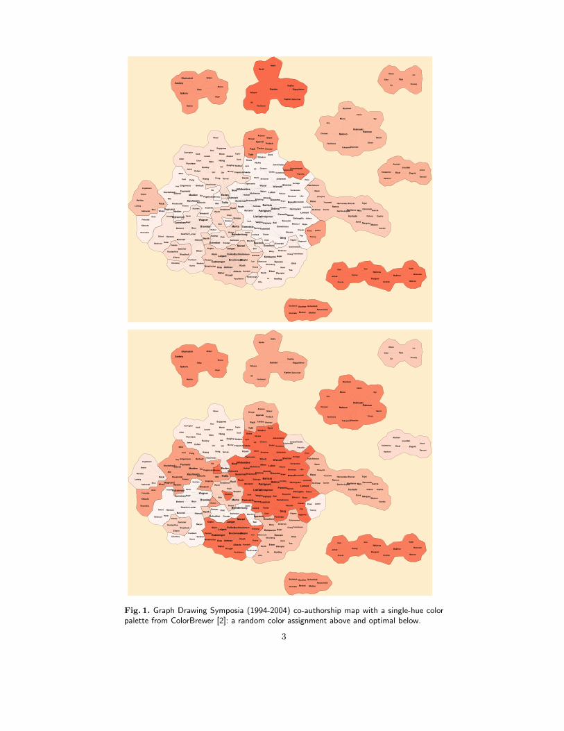
Fig. 1. Graph Drawing Symposia (1994-2004) co-authorship map with a single-hue colorpalette from ColorBrewer [2]: a random color assignment above and optimal below.

3

Not surprisingly, this is also an NP-Complete problem as shown in 1984 [10].Exact values for the antibandwidth of some of Hamming graphs [5], as well asfor meshes [14], hypercubes [12, 16], and complete k-ary trees for odd values ofk [3].

There have been definitions for a graph being k-edge Hamiltonian and k-vertex Hamiltonian in the literature [17], which are defined as the graph havinga Hamiltonian cycle after removing any k edges or vertices, respectively. Theseconcepts, though related, are different from our definition of k-Hamiltonian path,introduced in the next section.

3 Equivalence between Maximum Differential Coloringand Hamiltonian Path

Let the undirected graph of interest is G = {V,E}. We denote G as the com-plement of graph G, defined as G = {V, E}, where E = {{i, j}|i 6= j, i, j ∈V, and {i, j} /∈ E}. In other words, G is the graph containing all nodes in G,and all edges that are not in G. We now define the maximum differential coloringproblem formally.

Definition 1. A coloring of the nodes of G is a bijection c : V → {1, 2, . . . , |V |}.We denote the set of all colorings C(G).

Definition 2. A k-differential coloring of G is one in which the absolute coloringdifference of the endpoints for any edge is k or more. We denote the set ofall such k-differential colorings DC(G, k) = {c | c ∈ C(G), |c(i) − c(j)| ≥k for all {i, j} ∈ E}.

Definition 3. A graph is k-differential colorable if DC(G, k) 6= ∅.

Definition 4. If a graph is k-differential colorable, but not (k + 1)-differentialcolorable, it is said to have a differential chromatic number k, and denoted asdc(G) = k.

Definition 5. A Hamiltonian path of G is a bijection p : {1, 2, . . . , |V |} → V ,such that {p(i), p(i + 1)} ∈ E for all i = 1, 2, . . . , |V | − 1. We denote the set ofall Hamiltonian paths H(G).

The key insight in understanding the maximum differential coloring comesfrom observing a good differential coloring scheme. For example, in Figure 2(c),the minimum labeling difference between any two adjacency nodes is 3. Thismeans that any two nodes with labeling difference of ≤ 2 can not form an edge inG, in other word they must form an edge in the complement of the graph, shownin Figure 2(d). Therefore the list of nodes induced by this coloring scheme of G,with labels {1, 2, . . . , |V |}, forms a Hamiltonian path in G, shown in Figure 2(d)with orange arrows. Furthermore, this Hamiltonian path is such that any twonodes along the path with labeling difference of 2 are also connected by an edgeof G, shown in Figure 2(d) with dashed lines.

This observation leads to a natural extension of the concept of Hamiltonianpath, which we call k-Hamiltonian path.

4

1

3

1

1

3

3

1

3

1

3

3

1

1

3

3

1

3

3

1

3

1

1

3

1

1

2

4

3

5

6

7

8

9

(a) (b)

5

6

5

4

3

6

4

3

4

6

3

4

5

6

6

5

3

3

5

6

5

4

3

4

1

6

7

2

3

8

4

9

5

1

2

3

8

4

9

5

6

7

(c) (d)

Fig. 2. An illustration of the graph coloring problem and its relation to a k-Hamiltonianpath. A yellow to blue coloring scheme (indexed from 1 to 9) is used; nodes are labeled bycolor indices and edges are labeled with the absolute difference of of the adjacent nodes.(a) An input map. (b) The country graph G corresponding to the input map; note thatmany adjacent nodes have very similar colors. (c) An optimal 3-differential coloring of thecountry graph. (d) The complement graph G corresponding to G and a 2-Hamiltonianpath. The Hamiltonian path {1, 2, . . . , 9} is shown with orange arrows, and edges withlabeling difference of 2 are shown as blue dashed lines. Note that the 2-Hamiltonian pathof G is such that any two nodes of labeling difference ≤ 2 form an edge of G.

Definition 6. A k-Hamiltonian path (k ≥ 1) of G is a Hamiltonian path, suchthat each i-th node on the path is connected to the j-th node, if |i−j| ≤ k. We de-fine the set of k-Hamiltonian paths as H(G, k) = {p|p ∈ H(G), and {p(i), p(j)} ∈E if 0 ≤ i, j ≤ |V | and |i− j| ≤ k}. Clearly H(G) = H(G, 1).

Based on our previous discussion, we can relate the k-differential coloringproblem to that of finding a (k − 1)-Hamiltonian path.

Theorem 1. A k-differential coloring (k ≥ 2) of a graph G exists if and only ifa (k− 1)-Hamiltonian path exists in the complement of G, i.e., DC(G, k) 6= ∅ ifand only if H

(G, k − 1

)6= ∅. Furthermore, the inverse function of each element

of DC(G, k) is in H(G, k − 1

), and vice visa.

5

Proof. Suppose a k-differential coloring c exists for G. Define the path, p = c−1,so that it visits the vertices in the graph in order of their color index (i.e., the firstvertex is that with color 1, the second is that with color 2 and so on). Considertwo nodes u = p(i) and v = p(j) such that |i−j| ≤ k−1. Since the color differenceof these two nodes in the original graph, |c(u)−c(v)| = |i−j| ≤ k−1, by definitionof k-differential coloring (u, v) is not an edge of G, hence {u, v} = {p(i), p(j)} isan edge of G. It follows that p = c−1 is a (k − 1)-Hamiltonian path.

Conversely, suppose a (k − 1)-Hamiltonian path p exists for G. Define acoloring c = p−1, where the color index is given by the order in which a vertexappears in the path (i.e., color 1 is assigned to the first vertex along the path,color 2 to the second, and so on). Consider any edge {u, v} ∈ E. We prove that|c(u)− c(v)| ≥ k. Assume that |c(u)− c(v)| < k. Let i = c(u) and j = c(v), then|i − j| < k, and u = c−1(i) = p(i) and v = c−1(j) = p(j). By definition of a(k− 1)-Hamiltonian path, (u, v) must be an edge of G, which is a contradictionwith the fact that {u, v} ∈ E. It follows that |c(u) − c(v)| ≥ k, and so c = p−1

is a k-differential coloring of G. ut

This theorem immediately gives an upper bound for the differential chromaticnumber of a graph based on its maximum degree:

Corollary 1. A graph of maximum degree ∆(G) has a differential chromaticnumber of at most |V | −∆(G).

Proof. G must have a node with degree |V | − 1 − ∆(G), therefore H(G, |V | −∆(G)) = ∅, or by Theorem 1 DC(G, |V | −∆(G) + 1) = ∅. ut

A special case of differential coloring is finding a scheme with maximumdifference of 2 or more. Clearly:

Corollary 2. Finding a 2-differential coloring of a graph G is equivalent tofinding a Hamiltonian path of G.

Given the equivalence between 2-differential coloring and Hamiltonian path,a number of well known results for Hamiltonian path can immediately be usedto give results on 2-differential coloring.

Theorem 2. (Ore’s Theorem) A graph with more than 2 nodes is Hamiltonianif, for each pair of non-adjacent nodes, the sum of their degrees is |V | or greater

Corollary 3. A graph with more than 2 nodes is 2-differential colorable if, foreach pair of adjacent nodes, the sum of their degrees is |V | − 1 or less.

Theorem 3. (Dirac’s Theorem). A graph with more than 2 nodes is Hamilto-nian if each node has degree |V |/2 or greater.

Corollary 4. A graph with more than 2 nodes is 2-differential colorable if eachnode has degree |V |/2− 1 or less.

6

Corollaries 3-4 confirm the intuition that a sparser graph has a better chanceof being more differential colorable.3 The flip side of this intuition is that thecomplement graph needs to be denser. For a graph to be k-colorable, the com-plement graph must be well connected. The next theorem follows from a resultin [12]:

Theorem 4. The complement of a k-differential colorable graph is (k − 1)-connected.

Given the connection between finding a 2-differential coloring and a Hamil-tonian path, it is not difficult to prove directly that the maximum differentialcoloring problem is NP-Complete. An equivalent result was established in 1984in the context of the antibandwidth problem [10].

4 Algorithms for Maximum Differential Coloring

Theorem 1 provides a way to check whether a graph is k-differential colorable.The following kpath algorithm attempts to find a k-Hamiltonian path of G ={V, E} from a given node i. Before calling kpath the k-Hamiltonian path isinitialized as p = ∅. Each call to kpath recursively tries to add a neighbor tothe last node in the path, and checks that this maintains the k-path condition.If the condition is violated, the next neighbor is explored, or the algorithm backtracks. If a k-Hamiltonian path of G is found by the algorithm, we know thatthe graph G is (k + 1)-colorable.

This exact algorithm requires exponential time, making it impractical forlarge graphs, where heuristic algorithms might be a better choice. Gansner etal. [6] proposed a heuristic based on a relaxation of the discrete MaxMin problem(1) into a continuous maximization problem of 2-norm:

max∑{i,j}∈E

wij(ci − cj)2, subject to∑i∈V

c2i = 1 (2)

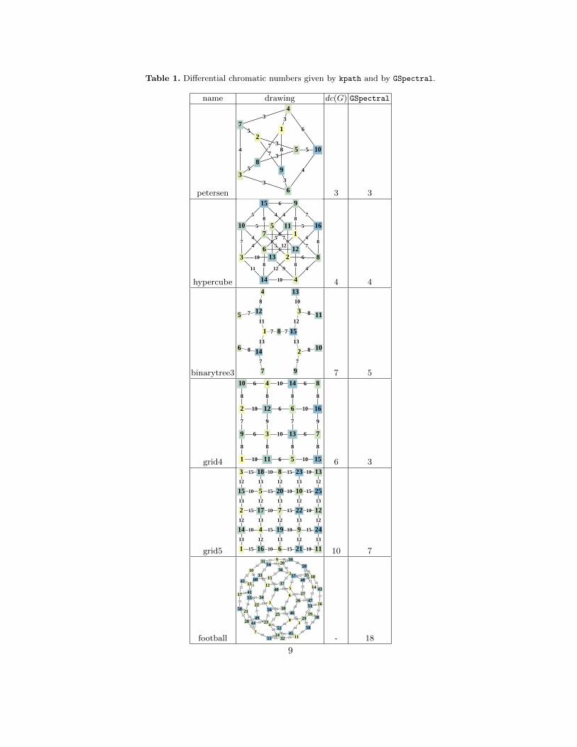
where c ∈ R|V |. This continuous problem is solved when c is the eigenvectorcorresponding to the largest eigenvalue of the weighted Laplacian of the graph.Once (2) is solved, the ordering of the eigenvector is used as an approximatesolution for the MaxMin problem. This is followed by a greedy refinement algo-rithm which repeatedly swaps pairs of vertices, provided that the swap improvesthe coloring scheme. We call this algorithm GSpectral (Greedy Spectral). Ta-ble 1 gives the chromatic number of some well known graphs found by kpath, aswell as an estimate of the differential chromatic number given by the GSpectral

algorithm. The GSpectral algorithm gets close to the optimal, though it findsthe actual optimal only twice. The exact algorithm kpath can be prohibitively

3 Even planar graphs, which have average degree less than 6, may be tough to colorwell. Consider a star graph, where one vertex is connected to every other vertex inthe graph. Regardless of the coloring, at least one pair of nodes will have a differenceof at most one, thus showing that dc(G) = 1.

7

Input: G, i, p (initialized to ∅ on first entry)Output: pif i ∈ p, or i is not connected with the last k nodes in p then

return ∅;endp = p ∪ {i};if |p| = |V | then

return p;endforeach neighbor node j of i do

if kpath(G, j, p) 6= ∅ thenreturn p;

end

endp = p− {i};return ∅;

Algorithm 1: kpath

expensive even for small graphs. For example, on the 60-node football graph(skeleton graph of a truncated icosahedron), one week of CPU time was notenough to find the exact differential chromatic number using kpath, whereasthe greedy spectral algorithm gives a lower bound of 18 in a few milli-seconds.We also tested GSpectral on larger grid graphs for which we believe that weknow the differential chromatic number (see Section 5). For grid10 and grid20

graph, it gives an estimate of 30 and 124, vs the actual differential chromaticnumbers of 45 and 190, respectively. In both case the CPU time for GSpectral

is less than 0.1 seconds.

5 Differential Chromatic Numbers of Special Graphs

Theorem 5. A line graph of n nodes has differential chromatic number ofbn/2c. A cycle graph of n nodes has differential chromatic number of b(n−1)/2c.

Proof. Consider a line graph with even number of nodes labeled in order withn/2+1, 1, n/2+2, 2, . . . , n, n/2; see Fig. 3(top). This labeling is clearly a n/2-differential coloring and it is easy to show that this is the best possible coloring.Take any labeling of this graph and consider the node labeled n/2. Regardless ofthe labels of its neighbor(s) this node must induce an edge difference of at mostn/2 achieved if the neighbor(s) is labeled n. Hence the differential chromaticnumber can not be more than n/2, that is, dc(G) = n/2 = bn/2c. A similarargument can be used in the case where the graph has an odd number of vertices;see Fig. 3 (bottom).

Now consider a cycle graph with an even number of vertices labeled in orderwith 1, n/2 + 1, 2, n/2 + 2, . . . , n/2, n; see Fig. 4(left). This labeling is clearlyn/2 − 1 = b(n − 1)/2c colorable and it is easy to show that this is the bestpossible coloring. Take any labeling of this graph and consider the node labeled

8

Table 1. Differential chromatic numbers given by kpath and by GSpectral.

name drawing dc(G) GSpectral

petersen

78

3

7

3

5

7

3

5

87

3

3

35

33

65

3

4

5

4

3 33

4

5

6

4

12

89

5

4

7

3

6

10

3 3

hypercube

6

712

8

6

54

8

5

6

12

97

6

4

812

10

9

84

10

11

7

1211

10

849

10

8

8

5

7

4

7

5

4

5

8

4

6

5

8

7

6

4

84

6

78

5

6

4

95

4

5

84

7

5

17

2 8133

14 4

510

6 12

915

11 16

4 4

binarytree3

7 7

11

13 13

12

8

7

8

7 7

8

8

10

81 15

12

14 2

3

4

5

6

7 9

10

11

13

7 5

grid4

8

10

8

7

6

7

8

10

8

6

10

8

6

6

8

9

10

10

9

8

6

6

8

10

6

8

10

10

8

7

6

6

7

8

10

10

8

6

10

8

6

8

9

10

9

8

6

8

1

9

2

10

11

3

12

4

5

13

6

14

15

7

16

8

6 3

grid5

13

15

13

12

10

12

13

15

13

12

10

12

15

15

12

10

10

12

13

15

15

13

12

10

10

12

13

15

15

13

10

10

13

15

15

13

12

10

10

12

13

15

15

13

12

10

10

12

15

15

12

10

10

12

13

15

15

13

12

10

10

12

13

15

15

13

10

10

13

15

13

12

10

12

13

15

13

12

10

12

1

14

2

15

3

16

4

17

5

18

6

19

7

20

8

21

9

22

10

23

11

24

12

25

13

10 7

football

31

24

21

35

26

45

44

18

20

21

21

21

2025

22

34

22

37

19

21

21

35

32

25

29

50

21

22

19

24

19

45

20

22

35

24

29

46

18

20

22

19

21

21

2223

21

25

30

21

33

28

20

4429

2121

21

22

4734

21

34

42

234521

27

21

27

30

21

29

22

33

25

29

27

33

29

3721

46

2019

22

52

2441

21

6

37

30

27

1

46

45

19

33

12

54

13

3

25

40

22

42

10

1734

41

60

4

51

29

16

2

38

58

26

31

15 48

20

47

5

52

32

823

1153

55

21

4928

9

36

18

14

50

43

56

24

44

7

39

57

59

35

- 18

9

5 6 5 6 5 6 5 6 56 1 7 2 8 3 9 4 10 5

6 5 6 5 6 5 6 5 6 51 7 2 8 3 9 4 10 5 11 6

Fig. 3. Optimal coloring of line graphs with 10 and 11 nodes.

5

9

45

4

5

45

4

5

1

62

7

3

8

4 9

5

10

6

5

5

6

56

5

6

5

65

1

7

2

83

9

4

10

5

11 6

Fig. 4. Optimal coloring of ring graphs with 10 and 11 nodes.

n/2. Regardless of the labels of its two neighbors this node must induce an edgedifference of at most n/2− 1 achieved if the first neighbor is labeled n and thesecond neighbor is 1 or n− 1. A similar argument can be used in the case wherethe graph has an odd number of vertices; see Fig. 4 (right). ut

Theorem 6. A grid graph of n × n nodes has differential chromatic number≥ 1

2n(n− 1).

Proof. If n is even, let m = n/2, we can color the grid as shown in Fig. 5. Dueto symmetry in numbering, only five labeling differences are possible: 2m2 −m, 2m2 − 1, 2m2, 2m2 + 1, 2m2 + m. The smallest is 2m2 −m = 1

2n(n − 1).For odd n there is a similar solution with only four label differences. ut

It turns out that 12n(n−1) is also an upper bound for the chromatic number of

the n×n grid graph, making this result tight [12]. It is informative to contrast anoptimally colored grid map with a grid map that uses the coloring induced by thelargest eigenvector; see Fig. 6. The eigenvector coloring provides good contrastbetween neighboring countries, particularly in the center. This indicates thatGSpectral might ineed be a good practical heuristic for large graphs.

6 Conclusion

In this paper we introduced the maximum differential graph coloring problemwhich arises in the context of map coloring. We described exact and heuristicalgorithms for this problem, and considered some special classes of graphs forwhich good solutions can be computed. We showed that this problem is relatedto that of find a k-Hamiltonian path. There is also a close relationship betweenthis problem and the antibandwidth problem.

We note that the results of this paper extend easily to the case when thereare more than |V | colors available: we can augment the graph with the same

10

2 m2- m2 m2

+ m

2 m2

2 m2- m

2 m2- 1

2 m2

2 m2- m2 m2

+ m

2 m2

2 m2+ 1

2 m2- m

2 m2

2 m2- m2 m2

+ m

2 m2

2 m2- m

2 m2

2 m2- m2 m2

+ m

2 m2- 1

2 m2

2 m2- m2 m2

+ m

2 m2

2 m2- m2 m2

+ m

2 m2

2 m2+ m

2 m2

2 m2+ m

2 m2

2 m2+ 1

2 m2+ m

2 m2

2 m2- m

2 m2- 1

2 m2

2 m2- 3

2 m2+ m - 3

2 m2- m

2 m2

2 m2+ m

2 m2

2 m2+ m

2 m2

2 m2+ 1

2 m2+ m

2 m2

1 2m2+m+1

2m2+1 m+1

2 2m2+m+2

2m2+2 m+2

m 2m2+2m

2m2+m 2m

2m+1

2m2+2m+1

2m+2

2m2+2m+2

3m

2m2+3m

2m2+3m+1

3m+1

2m2+3m+2

3m+2

2m2+4m

4m

2m2-2m+1

4m2-2m+1

2m2-2m+2

4m2-m-1

2m2-m

4m2-m

4m2-m+1

2m2-m+1

4m2-m+2

2m2-m+2

4m2

2m2

Fig. 5. Optimal coloring of n× n-grids for even n.

Fig. 6. Optimal grid map coloring (left) and one induced by the largest eigenvector (right).

number of isolated “dummy” nodes as there are extra colors. We further notethat countries that are not neighbors, but are nevertheless close (e.g., neighbor’sneighbor), can also be forced to have distinctive colors by adding additionaledges in the country graph linking these countries.

Throughout out the paper we have been assuming that the edge weights inthe country graph are uniform. That is, the importance of having a different colorbetween any pair of adjacent countries in the map is the same. We would alsolike to investigate ways to handle non-uniform weights, where more importancecan be placed on certain countries or certain types of adjacencies (e.g., long vs.short common borders).

11

7 Acknowledgments

We thank L’ubomır Torok for pointing out the related work on the antiband-width problem.

References

1. G. Blache, M. Karpinski, and J. Wirtgen. On approximation intractability of thebandwidth problem. Technical Report TR98-014, University of Bonn, 1998.

2. C. Brewer. ColorBrewer - Color Advice for Maps. www.colorbrewer.org.3. T. Calamoneri, A. Massini, L. Torok, and I. Vrto. Antibandwidth of complete

k-ary trees. Electronic Notes in Discrete Mathematics, 24:259–266, 2006.4. M. B. Dillencourt, D. Eppstein, and M. T. Goodrich. Choosing colors for geometric

graphs via color space embeddings. In 14th Symposium on Graph Drawing (GD),pages 294–305, 2006.

5. S. Dobrev, R. Kralovic, D. Pardubska, L. Torok, and I. Vrto. Antibandwidth andcyclic antibandwidth of hamming graphs. Electronic Notes in Discrete Mathemat-ics, 34:295–300, 2009.

6. E. R. Gansner, Y. F. Hu, and S. G. Kobourov. GMap: Visualizing graphs andclusters as maps. In IEEE Pacific Visualization Symposium (PacVis), pages 201–208, 2010.

7. E. R. Gansner, Y. F. Hu, S. G. Kobourov, and C. Volinsky. Putting recommen-dations on the map: visualizing clusters and relations. In 3rd ACM Conference onRecommender Systems (RecSys), pages 345–348, 2009.

8. Y. F. Hu and J. A. Scott. A multilevel algorithm for wavefront reduction. SIAMJournal on Scientific Computing, 23:1352–1375, 2001.

9. G. Kumfert and A. Pothen. Two improved algorithms for envelope and wavefrontreduction. BIT, 35:1–32, 1997.

10. J. Leung, O. Vornberger, and J. Witthoff. On some variants of the bandwidthminimization problem. SIAM Journal on Computing, 13:650, 1984.

11. C. Papadimitriou. The NP-Completeness of the bandwidth minimization problem.Computing, 16:263–270, 1975.

12. A. Raspaud, H. Schroder, O. Sykora, L. Torok, and I. Vrto. Antibandwidthand cyclic antibandwidth of meshes and hypercubes. Discrete Mathematics,309(11):3541–3552, 2009.

13. S. W. Sloan. An algorithm for profile and wavefront reduction of sparse matrices.International Journal for Numerical Methods in Engineering, 23:239–251, 1986.

14. L. Torok and I. Vrt’o. Antibandwidth of three-dimensional meshes. DiscreteMathematics, 310(3):505–510, 2010.

15. W. Unger. The complexity of the approximation of the bandwidth problem. InProceedings of the 39th Symposium on Foundations of Computer Science (FOCS),pages 82–91, 1998.

16. X. Wang, X. Wu, and S. Dumitrescu. On explicit formulas for bandwidth andantibandwidth of hypercubes. Discrete Applied Mathematics, 157(8):1947–1952,2009.

17. W. W. Wong and C. K. Wong. Minimum K-Hamiltonian graphs. Journal of GraphTheory, 8:155 – 165, 2006.

12