ON MEASURES OF ENTROPY ANDINFORMATION

ALFRPED RRNYIMATHEMATICAL INSTITUTE

HUNGARIAN ACADEMY OF SCIENCES

1. Characterization of Shannon's measure of entropy

Let d' = (pI, P2, - , pn,) be a finite discrete probability distribution, thatis, suppose pk _ O(k = 1, 2, * , n) and t-l Pk = 1. The amount of un-certainty of the distribution (P, that is, the amount of uncertainty concerningthe outcome of an experiment, the possible results of which have the probabili-ties PI, P2, * * * p,n, is called the entropy of the distribution (P and is usuallymeasured by the quantity H[(P] = H(p1, P2, * * pn), introduced by Shannon [1]and defined by

n 1(1.1) H(pl,p2,p p.) = E pk 1og2

k=1 Pk

Different sets of postulates have been given, which characterize the quantity(1.1). The simplest such set of postulates is that given by Fadeev [2] (see alsoFeinstein [3]). Fadeev's postulates are as follows.

(a) H(p1, P2, - pn) is a symmetric function of its variables for n = 2, 3,(b) H(p, 1 - p) is a continuous function of p for 0 < p _ 1.(c) H(1/2, 1/2) = 1.(d) H[tpI, (1 - t)pI, P2, * p.] = H(p1, P2, * Pn) + PIH(t, 1 -t)

for any distribution (P = (pI, P2, * * , pn) and for 0 _ t _ 1.The proof that the postulates (a), (b), (c), and (d) characterize the quantity

(1.1) uniquely is easy except for the following lemma, whose proofs up to noware rather intricate.LEMMA. Let f(n) be an additive number-theoretical function, that is, let f(n) be

defined for n = 1, 2, * and suppose(1.2) f(nm) = f(n) + f(m), n, m = 1, 2, .Let us suppose further that(1.3) lim [f(n + 1) - f(n)] = 0.

n-+-Then we have

(1.4) f(n) = c log n,where c is a constant.

547

548 FOURTH BERKELEY SYMPOSIUM: RENYI

This lemma was first proved by Erd6s [4]. In fact Erdos proved somewhatmore, namely he supposed, as is usual in number theory, the validity of (1.2) onlyfor n and m being relatively prime. Later the lemma was rediscovered by Fadeev.The proofs of both Erd6s and Fadeev are rather complicated. In this section wegive a new proof of the lemma, which is much simpler.PROOF. Let N > 1 be an arbitrary integer and let us put

(1.5) g(n) =f(n)- f(N)logn, n= 1, 2,*-

It follows evidently from (1.2) and (1.3) that

(1.6) g(nm) = g(n) + g(m), n, n = 1, 2, *

and that

(1.7) lim [g(n + 1) - g(n)] = 0.

We have further

(1.8) g(N) = 0.

Let us now put G(-1) = 0 and

(1.9) G(k) = max Ig(n)l, k = 0,1, --,Nk _n <Nk+1

and further,(1.10) k= max lg(n + 1) - g(n)1, k = 0,1, *-

Nk dn <Nk I

Clearly we have

(1.11) lim bk = 0-k-+w

Now we shall prove that

(1.12) lim 9(n) = 0.n- + log n

Since for Nk _ n < Nk+1, we have ig(n)I/log n _ G(k)/k log N, in order toprove (1.12) it is clearly sufficient to prove that

(1.13) lim G(k) = 0.k-*+ k

Now let n be an arbitrary integer and let k be defined by the inequalitiesNk _ n < Nk+I. Let us put n' = N[n/N] where [x] denotes the integral partof x; thus n' is the greatest multiple ofN not exceeding n. Then we have evidently0 _ n - n' < N and thus

(1.14) lg(n)I < 9g(n')I + E |g(l + 1) - g(l)I < Ig(n')I + Nbk.

By (1.6) and (1.8) we have

MEASURES OF ENTROPY AND INFORMATION 549

(1.15) g(n') = g ([N]) + g(N) = g ([n])and hence the inequalities Nk-l < [n/N] < Nk, together with (1.14), imply that(1.16) G(k) G(k-1) + N8k, k = 0,1,-.Adding the inequalities (1.16) for k = 0, 1, * *, m, it follows that

(1.17) G .< N (o+ Si+ + am)

Taking (1.11) into account, we obtain (1.13) and so (1.12). But clearly (1.12)implies

(1.18) lim f(n) _ f(N)n+. log n log N

As N was an arbitrary integer greater than 1 and the left side of (1.18) does notdepend on N, it follows that, denoting by c the value of the limit on the left sideof (1.18), we have(1.19) f(N) = clogN, N = 2,3,By (1.2) we have evidently f(1) = 0. Thus the lemma is proved.With a slight modification the above proof applies also in the case when the

validity of (1.2) is supposed only for relatively prime m and n. A previous versionof the above proof has been given by the author in [5]. The version given aboveis somewhat simpler than in [5].

Let us add some remarks on the set of postulates (a) to (d). Let us denote(-= (PI, P2, ,* pm) and Q = (ql, q2, *., q.) as two probability distributions.Let us denote by (I * Q the direct product of the distributions (I and Q, that is,the distribution consisting of the numbers pjqk with j = 1, 2, * , m; k = 1, 2,* * *, n. Then we have from (1.1)(1.20) H[6 * Q] = H[P] + H[Q],which expresses one of the most important properties of entropy, namely, itsadditivity: the entropy of a combined experiment consisting of the performanceof two independent experiments is equal to the sum of the entropies of thesetwo experiments. It is easy to see that one cannot replace the postulate (d) by(1.20) because (1.20) is much weaker. As a matter of fact there are many quan-tities other than (1.1) which satisfy the postulates (a), (b), (c), and (1.20). Forinstance, all the quantities

(1.21) Ha(p1, P2, p.) = _ log2 (kE1 pk)^

where a > 0 and a i 1 have these properties. The quantity Ha(pi, P2, * * p.)defined by (1.21) can also be regarded as a measure of the entropy of the dis-tribution (P = (pi, * , p,,). In what follows we shall call

Ha(Pl, P2, ... , pn) = Ha[(P]

550 FOURTH BERKELEY SYMPOSIUM: RENYI

the enlropy of order a of the distribution (Y. We shall deal with these quantitiesin the next sections. Here we mention only that, as is easily seen,

n 1(1.22) lim H.(pl, P2, p.) =_ pk log2

Thus Shannon's measure of entropy is the limiting case for a -* 1 of the measureof entropy H,,[G]. In view of (1.22) we shall denote in what follows Shannon'smeasure of entropy (1.1) by H1(p1, * * , p,n) and call it the measure of entropyof order 1 of the distribution. Thus we put

1(1.23) H1[(Y] = HI(pi, P2, P,,p7) = E pk 1og2 -

k=I pk

There are besides the quantities (1.22) still others which satisfy the postulates(a), (b), (c), and (1.20). For instance, applying a linear operation on Ha[6P] as afunction of a we get again such a quantity. In the next section we shall showwhat additional postulate is needed besides (a), (b), (c), and (1.20) to charac-terize the entropy of order 1. We shall see that in order to get such a character-ization of Shannon's entropy, it is advantageous to extend the notion of aprobability distribution, and define entropy for these generalized distributions.

2. Characterization of Shannon's measure of entropy of generalizedprobability distributions

The characterization of measures of entropy (and information) becomes muchsimpler if we consider these quantities as defined on the set of generalized prob-ability distributi(,ns. Let [Q, di, P] be a probability space, that is, Q an arbitrarynonempty set, called the set of elementary events; (1 a a-algebra of subsets of Q,containing Q itself, the elements of iM being called events; and P a probabilitymeasure, that is, a nonnegative and additive set function for which P(Q) = 1,defined on (B. Let us call a function t = t(co) which is defined for X Ez Q, whereQ1 E (B and P(Q1) > 0, and which is measurable with respect to (P, a generalizedrandom variable. If P(R1) = 1 we call t an ordinary (or complete) random variable,while if 0 < P(QI) < 1 we call t an incomplete random variable. Clearly, an in-complete random variable can be interpreted as a quantity describing the resultof an experiment depending on chance which is not always observable, only withprobability P(Q1) < 1. The distribution of a generalized random variable willbe called a generalized probability distribution. In particular, in the casewhen t takes on only a finite number of different values xl, x2, . . *, xn, the dis-tribution of t consists of the set of numbers pk = P{ = Xk} for k = 1, 2, -* *, n.Thus a finite discrete generalized probability distribution is simply a sequencepI, P2, * *pn of nonnegative numbers such that putting (P = (PI, P2, P* pn)and

(2.1) W(w) = Pk,k=1

MEASURES OF ENTROPY AND INFORMATION 551

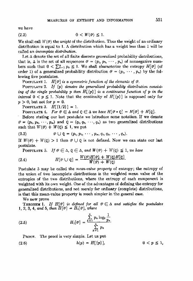
we have(2.2) 0 < W((P) < 1.

We shall call W(Q) the weight of the distribution. Thus the weight of an ordinarydistribution is equal to 1. A distribution which has a weight less than 1 will becalled an incomplete distribution.

Let A denote the set of all finite discrete generalized probability distributions,that is, A is the set of all sequences (P = (Pl, P2, . .. , pn) of nonnegative num-bers such that 0 < Ik=l pk < 1. We shall characterize the entropy H[GP] (oforder 1) of a generalized probability distribution 0P = (pi, * , pn) by the fol-lowing five postulates.POSTULATE 1. H[GY] is a symmetric function of the elements of (P.POSTULATE 2. If {p} denotes the generalized probability distribution consist-

ing of the single probability p then H[ {p}] is a continuous function of p in theinterval 0 < p < 1. Note that the continuity of H[{p}] is supposed only forp > 0, but not for p = 0.POSTULATE 3. H[{1/2}] = 1.POSTULATE 4. For (P E A and Q CE A we have H[(P * Q] = H[(P] + H[Q].Before stating our last postulate we introduce some notation. If we denote

(P = (pl, P2, . * pm) and Q = (qi, q2, , qn) as two generalized distributionssuch that W((P) + W(Q) _ 1, we put(2.3) (PU Q = (P1, P2, * pm, ql q2*q,).If W(() + W(Q) > 1 then (P U Q is not defined. Now we can state our lastpostulate.POSTULATE 5. If (P E A, Q E/A, and W((P) + W(Q) < 1, we have

(2.4) H[W U Q] = W((P)H[(p] + W(Q)H[Q].w((P) + W(Q)

Postulate 5 may be called the mean-value property of entropy; the entropy ofthe union of two incomplete distributions is the weighted mean value of theentropies of the two distributions, where the entropy of each component isweighted with its own weight. One of the advantages of defining the entropy forgeneralized distributions, and not merely for ordinary (complete) distributions,is that this mean-value property is much simpler in the general case.We now proveTHEOREM 1. If H[6(] is defined for all (P C A and satisfies the postulates

1, 2, 3, 4, and 5, then H[(P] = H1[(P], wheren 1

pk log2 -(2.5) H1[6P] = k

E Pkk=1

PROOF. The proof is very simple. Let us put(2.6) h(p) = H[{p}], 0 <p < 1,

552 FOURTH BERKELEY SYMPOSIUM: R]kNYI

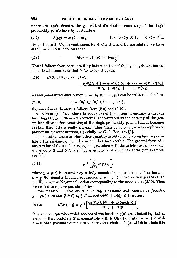
where {p} again denotes the generalized distribution consisting of the singleprobability p. We have by postulate 4

(2.7) h(pq) = h(p) + h(q) for 0 < p < 1; 0 < q ! 1.

By postulate 2, h(p) is continuous for 0 < p < 1 and by postulate 3 we haveh(1/2) = 1. Thus it follows that

1(2.8) h(p) = H[{p}] = log2-pNow it follows from postulate 5 by induction that if (Pl., (P2, * , (Pn are incom-plete distributions such that Ek- I W('k) < 1, then

(2.9) H[(P1 U (P2U *.* U()]w(QYI)H[(Pi] + w((92)H[6'2] + . + w((G)n)H[(GP]

w( '1) + W((P2) + * * * + w((6),,)

As any generalized distribution (P = (PI, P2, ..*. , pn) can be written in the form

(2.10) (9 = {PI} U {P2} U * U {Pn},

the assertion of theorem 1 follows from (2.9) and (2.10).An advantage of the above introduction of the notion of entropy is that the

term log2 (l/pk) in Shannon's formula is interpreted as the entropy of the gen-eralized distribution consisting of the single probability pk and thus it becomesevident that (1.1) is really a mean value. This point of view was emphasizedpreviously by some authors, especially by G. A. Barnard [6].The question arises of what other quantity is obtained if we replace in postu-

late 5 the arithmetic mean by some other mean value. The general form of amean value of the numbers xi, x2, *. , x. taken with the weights wi, w2, * * *, W.,where Wk > 0 and -21 Wk = 1, is usually written in the form (for example,see [7])

[ n

(2.11) g- [ Wkg(Xk)]E

where y = g(x) is an arbitrary strictly monotonic and continuous function andx = g-l(y) denotes the inverse function of y = g(x). The function g(x) is calledthe Kolmogorov-Nagumo function corresponding to the mean value (2.10). Thuswe are led to replace postulate 5 byPOSTULATE 5'. There exists a strictly monotonic and continuous function

y = g(x) such that if (P E A, Q E- A, and w(6') + w(Q) 1, we have

(2.12) H[P U Q] = g-1 [ww@)g(H[6 ]) + w(Q)g(H[Ql)

It is an open question which choices of the function g(x) are admissible, that is,are such that postulate 5' is compatible with 4. Clearly, if g(x) = ax + b witha # 0, then postulate 5' reduces to 5. Another choice of g(x) which is admissible

MEASURES OF ENTROPY AND INFORMATION 553

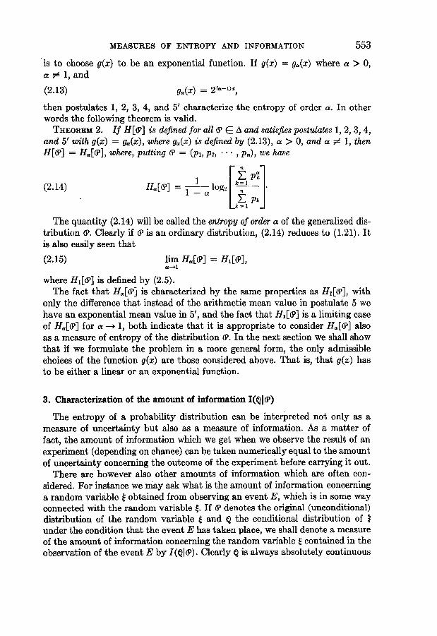
is to choose g(x) to be an exponential function. If g(x) = ga,(x) where a > 0,a 0 1, and

(2.13) ga(x) = 2

then postulates 1, 2, 3, 4, and 5' characterize the entropy of order a. In otherwords the following theorem is valid.THEOREM 2. If H[6'] is defined for all (P C A and satisfies postulates 1, 2, 3, 4,

and 5' with g(x) = g,(x), where g,,(x) is defined by (2.13), a > 0, and a # 1, thenH[6P] = Ha([P], where, putting (P = (pI, P2, , pn), we have

(2.14) H.[W] = 1 L PnLk=l

The quantity (2.14) will be called the entropy of order a of the generalized dis-tribution (P. Clearly if (P is an ordinary distribution, (2.14) reduces to (1.21). Itis also easily seen that(2.15) lim Hea[(6] = H1[6'],

a-*l

where H1[(P] is defined by (2.5).The fact that Ha[(P] is characterized by the same properties as H1[(P], with

only the difference that instead of the arithmetic mean value in postulate 5 wehave an exponential mean value in 5', and the fact that HI[(P] is a limiting caseof Ha[(Pl] for a -- 1, both indicate that it is appropriate to consider Ha[(P] alsoas a measure of entropy of the distribution (P. In the next section we shall showthat if we formulate the problem in a more general form, the only admissiblechoices of the function g(x) are those considered above. That is, that g(x) hasto be either a linear or an exponential function.

3. Characterization of the amount of information I(QI(P)

The entropy of a probability distribution can be interpreted not only as ameasure of uncertainty but also as a measure of information. As a matter offact, the amount of information which we get when we observe the result of anexperiment (depending on chance) can be taken numerically equal to the amountof uncertainty concerning the outcome of the experiment before carrying it out.

There are however also other amounts of information which are often con-sidered. For instance we may ask what is the amount of information concerninga random variable t obtained from observing an event E, which is in some wayconnected with the random variable t. If (P denotes the original (unconditional)distribution of the random variable t and Q the conditional distribution of Bunder the condition that the event E has taken place, we shall denote a measureof the amount of information concerning the random variable t contained in theobservation of the event E by I(Q16P). Clearly Q is always absolutely continuous

554 FOURTH BERKELEY SYMPOSIUM: R.iNYI

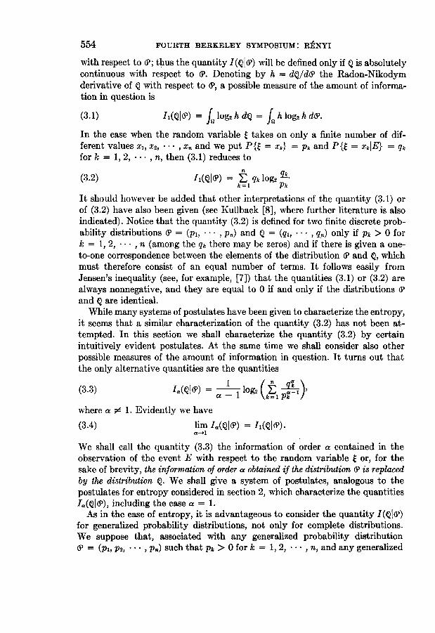
with respect to P1; thus the quantity I(QI(P) will be defined only if Q is absolutelycontinuous with respect to d'. Denoting by h = dQ/d6P the Radon-Nikodymderivative of Q with respect to (5, a possible measure of the amount of informa-tion in question is

(3.1) Ii(QI(P) = f log2hdQ = IQhlog2hdGP.

In the case when the random variable t takes on only a finite number of dif-ferent values x1, x2, * , x. and we put P{t = Xk} = Pk and P{t = xkfE} =qkfor k = 1, 2, *-- , n, then (3.1) reduces to

qk.(3.2) Ii(QI(P) = k qk 1og2p

It should however be added that other interpretations of the quantity (3.1) orof (3.2) have also been given (see Kullback [8], where further literature is alsoindicated). Notice that the quantity (3.2) is defined for two finite discrete prob-ability distributions aP = (pi, * *, pn) and Q = (ql, * * *, q.) only if Pk > 0 fork = 1, 2, -- , n (among the qk there may be zeros) and if there is given a one-to-one correspondence between the elements of the distribution d' and Q, whichmust therefore consist of an equal number of terms. It follows easily fromJensen's inequality (see, for example, [7]) that the quantities (3.1) or (3.2) arealways nonnegative, and they are equal to 0 if and only if the distributions (Pand Q are identical.

While many systems of postulates have been given to characterize the entropy,it seems that a similar characterization of the quantity (3.2) has not been at-tempted. In this section we shall characterize the quantity (3.2) by certainintuitively evident postulates. At the same time we shall consider also otherpossible measures of the amount of information in question. It turns out thatthe only alternative quantities are the quantities

(3.3) Ia(Q1(P) = a _1 lg2 (k ak)

where a F# 1. Evidently we have(3.4) lim Ia(Q1(P) Ii(QI(P)-We shall call the quantity (3.3) the information of order a contained in theobservation of the event E with respect to the random variable t or, for thesake of brevity, the information of order a obtained if the distribution (P is replacedby the distribution Q. We shall give a system of postulates, analogous to thepostulates for entropy considered in section 2, which characterize the quantitiesIa(I(P), including the case a = 1.As in the case of entropy, it is advantageous to consider the quantity I(Q1(P)

for generalized probability distributions, not only for complete distributions.We suppose that, associated with any generalized probability distribution(P = (Pl, P2, ... , pn) such that Pk > 0 for k = 1, 2, .* .. , n, and any generalized

MEASURES OF ENTROPY AND INFORMATION 555

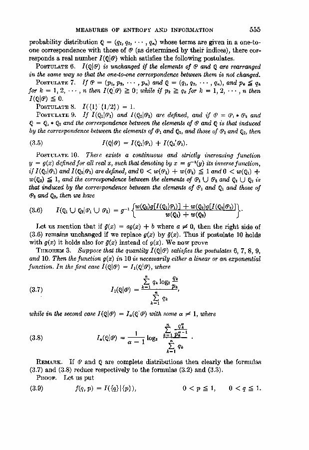
probability distribution Q = (ql, q2, * - *, q,) whose terms are given in a one-to-one correspondence with those of (P (as determined by their indices), there cor-responds a real number I(Q1I') which satisfies the following postulates.POSTULATE 6. I(QI16) is unchanged if the elements of (P and Q are rearranged

in the same way so that the one-to-one correspondence between them is not changed.POSTULATE 7. If (P = (pl, P2, * - , pn) and Q = (ql, q2, .* .. , q.), and pk . qk

for k = 1, 2, , n thenl(QI() > O; while if pk > qkfor k = 1, 2, * , n thenI(QIcj) _ 0.POSTULATE 8. I({1}1{1/2}) = 1.POSTULATE 9. If I(Q1I(P1) and I(Q216R2) are defined, and if ( = (P * (P2 and

Q = Q, * Q2 and the correspondence between the elements of (P and Q is that inducedby the correspondence between the elements of (P, and Ql, and those of P2 and Q2, then

(3.5) I(Q!(P) = I(QlI(Pl) + I(Q216P2)-POSTULATE 10. There exists a continuous and strictly increasing function

y = g(x) defined for all real x, such that denoting by x = g-l(y) its inverse function,if I(Q I'lE) and I(Q21(P2) are defined, and 0 < w(611) + w((12) _ 1 andO < w(Q1) +w(Q2) _ 1, and the correspondence between the elements of (Pi U P2 and Ql U Q2 isthat induced by the correspondence between the elements of (1P and Qi and those of(P2 and Q2, then we have

(3.6) I(Q1 U Q216(1 U (2) = g-1 {w(Q) W[I(Ql)] + W(Q2) i f2)}Let us mention that if g(x) = ag(x) + b where a #5 0, then the right side of

(3.6) remains unchanged if we replace g(x) by g(x). Thus if postulate 10 holdswith g(x) it holds also for g(x) instead of g(x). We now proveTHEOREM 3. Suppose that the quantity I(Qj(P) satisfies the postulates 6, 7, 8, 9,

and 10. Then the function g(x) in 10 is necessarily either a linear or an exponentialfunction. In the first case I(QI(P) = I,(Q! P), where

n IE_ qk 1og2_

(3.7) I (Q(p) = pk

E qkk=1

while in the second case I(Q16') = Ia(QI(P) with some ac 1, where

n ag1T__k

___ ~~k lk(3.8) Ia(QI(P) = 10g2E qkk=1

REMARK. If ( and Q are complete distributions then clearly the formulas(3.7) and (3.8) reduce respectively to the formulas (3.2) and (3.3).PROOF. Let us put

(3.9) f(q, P) = I({Q}{p}), 0 < p _ 1, 0 <q <1.

556 FOURTH BERKELEY SYMPOSIUM: RENYI

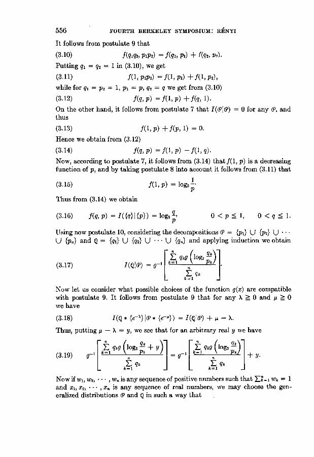
It follows from postulate 9 that

(3.10) f(q,q2, PlP2) = f(ql, pi) + f(q2, p,).Putting q1 = q2 = 1 in (3.10), we get

(3.11) f(l,p1p2) ef(1, pI) + f(1,p2),while for q1 = P2 = 1, pi = p, q2 = q we get from (3.10)(3.12) f(q, p) =f(l, p) + f(q, 1).On the other hand, it follows from postulate 7 that I(PI (P) = 0 for any (P, andthus

(3.13) f(l, p) + f(p, 1) = 0.

Hence we obtain from (3.12)(3.14) f(q, p) = f(l, p) - f(l, q).Now, according to postulate 7, it follows from (3.14) that f(l, p) is a decreasingfunction of p, and by taking postulate 8 into account it follows from (3.11) that

(3.15) f(l,p) =log2P

Thus from (3.14) we obtain

(3.16) f(q, p) = I({q}{p}) = log2 0 < p < 1, 0 < q _ 1.p

Using now postulate 10, considering the decompositions (P = {pl} U {P2} U ...

U {p.} and Q = {ql} U {q2} U ... U {qn} and applying induction we obtain

(3.17) I(WP) = P-1 k)1_ Qk=

Now let us consider what possible choices of the function g(x) are compatiblewith postulate 9. It follows from postulate 9 that for any X > 0 and A >_ 0we have

(3.18) I(Q * {e-}f1(P * {e-"}) = I(Q|j) + A- X.Thus, putting .t - X = y, we see that for an arbitrary real y we have

E qkg (log2- + y) F qkg log,,(3.19) g- k n ] g- k=I ng +q .

[ qk F_ qk

Now if w1, w2, * , w. is any sequence of positive numbers such that _k = 1 Wk = 1and x,, x2, . . *, Xn is any sequence of real numbers, we may choose the gen-eralized distributions (P and Q in such a way that

MEASURES OF ENTROPY AND INFORMATION ,557

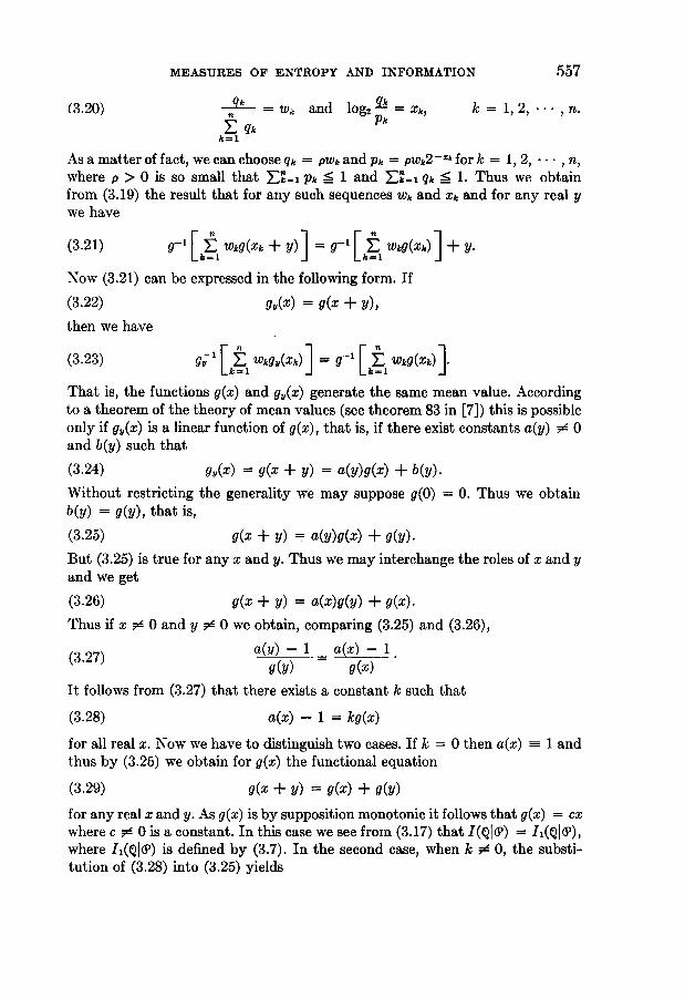
(3.20) -qk= wc and log2 =XkXk, k =1, 2, **,n.n PE qk Pk

k=1

As a matter of fact, we can choose qk = PWk and pk = pWk2-zk for k = 1, 2, * n,where p > 0 is so small that F2t-.1 Pk : 1 and X.-1 qk . 1. Thus we obtainfrom (3.19) the result that for any such sequences Wk and Xk and for any real ywe have

(3.21) [l Wkg(Xk + Y)] g [k Wkg(Xk)] + YiNow (3.21) can be expressed in the following form. If

(3.22) gv(x) = g(x + y),then we have

(3.23) gy [E Wk9y(Xk)] = g [E wkg(xk)].k=l k-1

That is, the functions g(x) and gy(x) generate the same mean value. Accordingto a theorem of the theory of mean values (see theorem 83 in [7]) this is possibleonly if gy(x) is a linear function of g(x), that is, if there exist constants a(y) # 0and b(y) such that

(3.24) gy(x) = g(x + y) = a(y)g(x) + b(y).Without restricting the generality we may suppose g(0) = 0. Thus we obtainb(y) = g(y), that is,

(3.25) g(x + y) = a(y)g(x) + g(y).But (3.25) is true for any x and y. Thus we may interchange the roles of x and yand we get

(3.26) g(x + y) = a(x)g(y) + g(x).Thus if x 5 0 and y 't 0 we obtain, comparing (3.25) and (3.26),(3.27) a(y) -1 a

g(y) g(x)It follows from (3.27) that there exists a constant k such that

(3.28) a(x) - 1 = kg(x)

for all real x. Now we have to distinguish two cases. If k = 0 then a(x) =_ 1 andthus by (3.25) we obtain for g(x) the functional equation

(3.29) g(x + y) = g(x) + g(y)for any real x and y. As g(x) is by supposition monotonic it follows that g(x) = cxwhere c # 0 is a constant. In this case we see from (3.17) that I(Qk6P) = Ii(QjIP),where II(Qc6P) is defined by (3.7). In the second case, when k # 0, the substi-tution of (3.28) into (3.25) yields

558 FOURTH BERKELEY SYMPOSIUM: RENYI

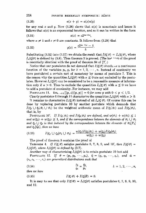
(3.30) a(x + y) = a(x)a(y)for any real x anid y. Now (3.28) shows that a(x) is monotoniic and hence itfollows that a(x) is an exponential function, and so it can be written in the form(3.31) a(x) = c2a-I'xwhere a 5z 1 and c $R 0 are constants. It follows from (3.28) that

(3.32) g(x) = C2(a 1)x - 1k

Substituting (3.32) into (3.17) we obtain the result that I(QIc) = I.(Q I ), whereIa(QkP) is defined by (3.8). Thus theorem 3 is proved. (The lass -.rt of the proofis essentially identical with the proof of theorem 84 of [7].)

Notice that our postulates do not demand that I(QIY) shoulu ue a continuousfunction of the variables Pk, qk for k = 1, 2, * * *, n. Instead of continuity wehave postulated a certain sort of monotony by means of postulate 7. This isthe reason why the quantities Ia(Q16P) with a _ 0 are not excluded by the postu-lates. However 1(QI(P) can be considered to be a reasonable measure of informa-tion only if a > 0. Thus to exclude the quantities Ia(QIP) with a < 0 we haveto add a postulate of continuity. For instance, we may addPOSTULATE 11. limrn>+o [(p, E)I(p, p)] = Ofor some p with 0 < p < 1/2.Clearly postulates 6 through 11 characterize the quantities Ia(QI P) with a > 0.It remains to characterize II(QIG6) instead of all Ia(QfP). Of course this can be

done by replacing postulate 10 by another postulate which demands thatI(Q1 U Q21l(l U (P2) be the weighted arithmetic mean of I(Q1|(Pj) and I(Q21WP2),that is, byPOSTULATE 10'. If I(QjKPY) and I(Q21(P2) are defined, and w(QP) + w(Q2) _ 1

and w(Q1) + w(Q2) < 1, and if the correspondence between the elements of (Gl U (i2and Ql U Q2 is that induced by the correspondence between the elements of (P1[P2]and Q,[Q2], then we have

(3.33) I(Q1 U Q21GN U 6P2) = W(Q1)I(Q1jrY1) + w(Q2)I(Q2IY2).W(Q1) + W(Q2)

The proof of theorem 3 contains the proof ofTHEOREM 4. If I(QIP) satisfies postulates 6, 7, 8, 9, and 10', then I(QIP) =

II(Q16P), where I1(Q(YP) is defined by (3.7).Another way of characterizing I1(QIP) is to retain postulate 10 but addPOSTULATE 12. If (3 = (PI, P2, * pn), Q = (ql, q2, ** X qn), and aR =

(r1, r2, * rn) are generalized distributions such that

(3.34) rk qk k = 1, 2, n,qk Pkthen we have

(3.35) I(Qjr) + I(Q|R) = 0.It is easy to see that only I(QI(W) = Ii(QJ61) satisfies postulates 6, 7, 8, 9, 10,

and 12.

MEASURES OF ENTROPY AND INFORMATION 559

4. Information-theoretical proof of a limnit theorem on Markov chainsThe idea of using measures of information to prove limit theorems of prob-

ability theory is due to Linnik [9]. In this section we shall show how this methodworks in a very simple case.

Let us consider a stationary AMarkov chain with a finite number of states.Let P,k for j, k = 1, 2, - *, N denote the transition probability in one step andp(k) the transitioni probability in n steps from state j to state k. We restrictourselves to the simplest case when all transition probabilities pik are positive.In this case, as is well knowin, we have

(4.1) lim pA; = Pk, j, k = 1, 2, N,n-+.

where the limits Pk are all positive and satisfy the e(quationsIV

(4.2) E pjpjk = Pk, k = 1, 2, N,j=1

andA'

(4.3) Y = 1.k=1

Our aim is to give a new proof of (4.1) by the use of the measure of informationII(QV6P). The fact that the system of e(quations (4.2) and (4.3) has a solution(Pl, P2, * * , pv) consisting of positive iiumbers can be deduced by a well-knowntheorem of matrix theory. In proving (4.1) we shall take it for granted that such

() (n) p(n,)numbers Pk exist. Let us put (Y = (pI, P2, PN) and (pj) = (pj(l')) pj2 N*pn)and consider the amounts of information

N (t

(4.4) I1((5 lCI) = E p, log2 pk=1 Pk

According to the definitioni of transitioln probabilities, we haveN

(4.5) Pi(" = p pIk-

Now let us introduce the notation

(4.6) Xra P lPk

The probabilistic meaninlg of the numbers 7rlk iS clear: I1k is the conditionalprobability for the chain's being in state 1, under the condition that at the nextstep it will be in state k, provided that the initial distribution is the stationarydistribution given by the numbers PI, P2, *.. , PN. The conditional probabilitiesIrlk are often called the "backward" transition probabilities of the Markovchain. Now w^e have clearly 1 =lTrk = 1 for k = 1, 2, * * ,N and by (4.5)

N FN Ipl )] FN[E)(4.7) I1(6,j1n±l)1PG) = k Pk 71k 10g2 Irlk (IJ j

560 FOURTH BERKELEY SYMPOSIUM: RE'NYIApplying Jensen's inequality [7] to the convex function x log2 x, for each valueof k, we obtain from (4.7)

NV NV (n') (n)

(4.8) Ii(6Yj( j(P) - EI pk E 7rIk plog2 p

Taking into account the fact thatN

(4.9) k Pk7rIk ==k=1

it follows from (4.8) that

(4.10) (+llP< ((85)Thus the sequence I,(GJ(n)1j() is decreasing, and as I1(Gf)1(P) > 0, the limit(4.11) L = lim I,(6jn) 1(P)exists. We shall show now that L = 0 and simultaneously that (4.1) holds. Asthe number of states is finite, we can find a sequence ni < n2 < ... < n, < ...

of positive integers, such that the limits(4.12) lim pj5s8) = q, k k = 1, 2, * , N,

exist. As EkN= 1 pjk) = 1, we have evidentlyN

(4.13) _= 1 .

k=1

Let us put furtherN

(4.14) = qajlplk, k = 1, 2, * , N,

and put for the sake of brevity Qj = (qjil, qj2, * , qjN) and Qf = (qfl, qj2, **, qjN).Clearly we have(4.15) lim I1((61`10(P) = Ii(QjI,) = L

and(4.16) lim II((P5nb+1)I() = l(Q>IG') = L-

Again using Jensen's inequality, exactly as in proving (4.10), we have

(4.17) I,(QI6) = pk E TIk (pj)] log2 [,2Erzk( )] _ I(QVP)

with equality holding in (4.17) only if qj /pI = c for 1 = 1, 2, * , N, where c

is a constant. But by (4.16) it follows that there is equality in (4.17), and thuswe have(4.18) qjl = cpl, 1 = 1, 2, ,N.

Notice that here we have made essential use of the supposition that all Pik and

MIEASURES OF ENTROPY AND INFORMATION 561

thus all 7rIk are positive. In view of (4.3) and (4.13) the constant c in (4.18) isequal to 1, and tlherefore j = (Y. It follows from (4.15) that

(4.19) L = I,(6<0) = 0.We have inicideentally proved that (4.1) holds, as wi-e have sholon that iffor an arbitrary subsequence n, we have (4.12) then niecessarily q,1 = pl for1 = 1, 2, * * , N. But if (4.1) were false, we could finid a subse(ullence n,, ofinitegers such that (4.12) holds with qjl 0 pi.

It is clear from the above proof that inistead of the quianitities (4.4) \Ne colilhave used the analogous sums

(4.20) k Pk(wheref(x) is any function such that xf(x) is strictly conivex. 'l1hus for instancewe could have taken f(x) = xc-I' with a > 1 or f(x) = -x- I with 0 < a < 1.This means that instead of the measure of information of the first order, wN-ecould have used the measure of information of any order a > 0, and deduce (4.1)from the fact that lim + I ((Y8(P) = 0.

In proving limit theorems of probability theory by considerinig nmeasures ofiiiformation, it is usually an advantage that one cani choose between differenitmeasures. In the above simple case each measure Ia(Ql v)was equally suitable,but in other cases the quantity I2(Ql(), for example, is more easily dealt wVithtthan the quantity Il(QIW). The author intends to return to this question, b)ygiving a simplified versioni of Linnik's iniformation-theoretical proof of the cell-tral limit theorem, in another paper.

REFEIRENCES

[1] C. E. SHANNON andl W. WEAVER, 7The Mathemtiatical Theory of Comntnunication, Urbana,University of Illinois Press, 1949.

[2] D. K. FADEEV, "Zum Begriff der Entrlopie ciner endlichen Wahrseheililhlikeitss(chernas,"A rbeiten zu1- Infor,nationstheorie I, Berlini, D)eutscher Verlag der Wissensehaf ten, 1957,pp. 85-90.

[3] A. FEINSTEIN, Foun(lations of Inforniation Theory, New York, McGraw-Hill, 1958.[4] P. ERDO1S, "On the distribution function of additive functions," Ann. of Mlath., Vol. 47

(1946), pp. 1-20.[5] A. RENYi, "On a theorem of Erd6s and its application in information theory," Mlathematica,

Vol. 1 (1959), pp. 341-344.[6] G. A. BARNARD, "The theory of information," J. Roy. Statist. Soc., Ser. B, Vol. 13 (1951),

pp. 46-64.[7] G. H. HARDY, J. E. LITTLEWOOD, and G. P6LYA, Intequalities, Camiibridge, Cambridge

University Press, 1934.[8] S. KULLBACK, Inform ation Theory and Statistics, New York, Wiley, 1959.[9] Yu. V. LINNIK, "An information theoretical proof of the central limit theorem on Lindeberg

conditions," 7'eor. Veroyatnost. i Primenen., Vol. 4 (1959), pp. 311-321. (In Russian.)