Abstract We study the L p-mean distortion functionals,
E p[ f ] =∫∫
D
Kp(z, f ) dz, f|S = f0
for Sobolev self homeomorphisms of the unit disk D with prescribed boundary valuesf0 : S → S and pointwise distortion function K = K(z, f ). Here we discuss aspectsof the existence, regularity and uniqueness questions for minimisers and discuss thediffeomorphic critical points of Ep presenting results we know and making some
Communicated by Bruce Palka.
T. Iwaniec was supported by the NSF grant DMS-1301558 and the Academy of Finland project 1128331.G. J. Martin was supported by the N. Z. Marsden Fund and Magdalen College, Oxford University,J. Onninen was supported by the NSF grant DMS-1301570.
T. IwaniecSyracuse University, Syracuse, USA
T. Iwaniec · J. OnninenUniversity of Helsinki , Helsinki, Finland
G. Martin (B)Massey University, Auckland, New Zealande-mail: [email protected]
G. MartinMagdelen College, Oxford University, Oxford, UK
J. OnninenUniversity of Jyväskylä, Jyväskylä, Finland
123
T. Iwaniec et al.
conjectures. Remarkably, smooth minimisers of the L p-mean distortion functionalshave inverses which are harmonic with respect to a metric induced by the distortionof the mapping. From this we are able to deduce that the complex conjugate Beltramicoefficient of a smooth minimiser is locally quasiregular and we identify the quasilinearequation it solves. This has other consequences such as a maximum principle for thedistortion.
Keywords Mean distortion minimisers · Harmonic mappings · Calculus ofvariations
Let � and �′ be bounded Jordan domains in the complex plane C and f : �onto−→ �′
a homeomorphism of Sobolev class W 1,1loc (�, C). We always assume our homeomor-
phisms are orientation preserving.A Sobolev mapping f : � → C is said to have finite distortion if
‖D f (z)‖2 � K (z) J (z, f ) almost everywhere (1)
for some measurable function 1 � K (z) < ∞. Here,
‖D f (z)‖2 def==| fz |2 + | fz̄ |2
(normalized Hilbert–Schmidt norm) and
J (z, f )def== det D f (z) = | fz |2 − | fz̄ |2.
The smallest such K (z) will be denoted by K(z, f ) and is called the distortion functionof f . Thus, under the assumption (1), we have
K(z, f ) = ‖D f (z)‖2
J (z, f ), if J (z, f ) > 0, and K(z, f ) = 1, if J (z, f ) = 0. (2)
We study homeomorphisms f : �onto−→ �′ of finite distortion K(·, f ) ∈ L p(�, λ),
1 � p � ∞, where λ : � → R+ is a positive weight. Denote
Ep,λ[ f ] =∫∫
�
[ K(z, f ) ]p λ2(z) dz, Ep[ f ] def== Ep,1[ f ].
123
On Minimisers of L p-mean Distortion
We will always assume that λ ∈ C1(�). For our study we will consider the followingclasses of homeomorphism f : �
onto−→ �′ with finite distortion:
QC p,λ(�,�′) = { f : Ep,λ[ f ] < ∞}, QC p(�,�′) = QC p,1(�,�′)QC∞(�,�′) = QC(�,�′), the quasiconformal mappings
For this paper, the case of most interest will be � = �′ = D, the unit disk.
1.1 Mappings of Smallest L p-Mean Distortion
Suppose we are given f0 ∈ QC p,λ(�,�′) as datum for a minimisation problem.
Definition 1.1 A homeomorphism f ∈ QC p,λ(�,�′) is said to be Dirichletextremal, or L p-extremal, if
∫∫
�
Kp(z, f ) λ2(z) dz �
∫∫
�
Kp(z, h) λ2(z) dz (3)
for every h ∈ QC p,λ(�,�′) which coincides with f0 on ∂�.
A homeomorphism f : �onto−→ �′, with Ep,λ[ f ] < ∞, is said to be an absolute
minimiser if (3) holds for every homeomorphism h : �onto−→ �′, with Ep,λ[h] < ∞,
regardless of the boundary values (which may not even exist).
Of course, if �′ is conformally equivalent to �, then the absolute minimiser isa conformal mapping. The question of existence of an absolute minimiser thereforepertains to problems where there are conformal moduli associated to the domain �,such as doubly or multiply connected domains in which case one might add conditionssuch as requiring the minimiser and the data to be in same homotopy class. The absoluteminimizers of such problems where the boundary values are not prescribed are knownin non-linear elasticity as traction-free deformations.
1.2 The Problem
The problem we primarily consider here is the following: given a homeomorphismf0 ∈ QC p,λ(�,�′) investigates the existence and the uniqueness of a Dirichletextremal mapping. Then establish the precise regularity of such a mapping shouldit exist.
For two particular values of p, p = 1 and p = ∞, many results are known.For p = ∞ the theory concerns extremal quasiconformal mappings and Teichmüllertheory and obviously has wide connections in mathematics. For the less well-knowncase p = 1, see [1–4]. These ideas have various applications in non-linear elasticityand material science, see for instance [5,6]. We will take a moment to recall whatthese results are.
123
T. Iwaniec et al.
1.3 p = ∞
This is the theory of extremal quasiconformal mappings. We note that as p → ∞⎛⎝
∫∫
�
Kp(z, f )λ2(z) dz
⎞⎠
1/p
→ ‖K(·, f )‖L∞(�), (4)
so there is no dependence on λ. It is well-known that there is a homeomorphismf : D
onto−→ D with the smallest maximal distortion if and only if f0 : ∂Donto−→ ∂D is
quasisymmetric [7]; that is, there is an increasing η : [0,∞] → [0,∞] such that
| f0(ζ1) − f0(ζ2) || f0(ζ1) − f0(ζ3) | � η
( |ζ1 − ζ2||ζ1 − ζ3|
), ζ1, ζ2, ζ3 ∈ ∂D. (5)
The quasiconformal map with the smallest maximum distortion is not always unique,but is in many special cases of interest, such as mappings between Riemann surfaces.This is Teichmüller’s theorem, see [8, Sect. 2.6.4] and [9]. An important class ofquasiconformal mappings with the smallest maximal distortion, called Teichmüllerextremals, consists of homeomorphisms f whose distortion K(z, f ) is constant andthe Beltrami coefficient μ f (z) = kϕ̄/|ϕ|, for a certain holomorphic function ϕ anda real k ∈ [0, 1). For Teichmüller extremals, there is an associated holomorphicquadratic differential which gives, away from its singularities, local co-ordinates inwhich the minimiser is linear. But not every quasiconformal extremal is a Teichmüllerextremal [10,11] and sometimes Teichmüller extremals do not exist [12]. Obviously,for a Teichmüller extremal map we have
∫
D
ϕ(z)μ f (z) dz = k = ||μ f ||∞,
where ϕ is a holomorphic function of L1-norm equal to 1. However, for a generalextremal quasiconformal map we need only to have a sequence {ϕ j } of holomorphicfunctions in L1(D), normalized by ||ϕ j ||L1(D) = 1, such that.
limj→∞
∫
D
ϕ j (z) μ f (z) dz = ||μ f ||L∞(D) (6)
Such a sequence {ϕ j } is referred to as a Hamilton sequence. This can be viewed as aweak form of the Teichmüller condition for extremals.
Much more can be found in the work of Reich and Strebel [13,14] and elsewhere.This raises many interesting questions about the behaviour of the L p-extremals forquasisymmetric boundary values as p → ∞, some of which we discuss below.
123
On Minimisers of L p-mean Distortion
1.4 p = 1
The transition to the study of the inverse map, first exploited in this context in [3], butsee [15, Sect. 21.1.4], and which we discuss more carefully later, leads to the theoryof harmonic mappings. When λ(z) ≡ 1 then a boundary homeomorphism f0 : S → S
admits an extension to f ∈ QC1(D, D) if and only if
∫∫
S×S
|log | f0(ζ ) − f0(ξ)|| |dζ | |d ξ̄ | < ∞. (7)
In fact, for such extensions the smallest L1-mean distortion is given explicitly bymeans of the integral
∫∫
D
K(z, f ) dz = − 1
π
∫∫
S×S
log| f0(ζ ) − f0(ξ)| dζ dξ̄ .
This unique minimal extension is a smooth diffeomorphism whose inverse g =f −1 : D → D is harmonic. Using work of Pavlovich [16] this minimiser is quasicon-formal if and only if f0 : S → S is bilipschitz. See [3, Thms. 10.12, 11.1] for theseand related facts.
1.4.1 Harmonic Mappings with Respect to General Metrics
For more general weights λ we need to recall the notion of a harmonic mapping withrespect to other metrics conformally equivalent to the Euclidean metric. This willalso be important to us later. Let � and �̃ be domains in the complex plane C. Weadopt the notation we will use later and write the dependent variable as w ∈ �̃. Asmooth real-valued function ρ : � → R+ defines a conformal metric ρ(z)|dz| on �.A mapping g : �̃ → (�, ρ), z = g(w), of class C2(�̃) is harmonic (or ρ-harmonic)if it is a solution to the non-linear second-order equation, called the tension equation,
∂2g
∂w∂w̄+ ρz(g)
ρ(g)
∂g
∂w
∂g
∂w̄= 0, g = g(w). (8)
Note that this criterion does not depend on the conformal structure of the domain ofdefinition of the mapping g, but it does depend on the conformal change of variables inthe target space �. The relevance here is that these are the Euler–Lagrange equationsfor the critical points of the functional
g �→∫
�̃
‖Dg‖2λ2(g) dw; precisely, with λ(z) = ρ(z). (9)
123
T. Iwaniec et al.
After the change of variables f = g−1, as discussed above, (9) becomes the functional
f �→∫
�
K(z, f )λ2(z) dz (10)
which is the weighted case with p = 1, of interest to us.
Remark 1.1 It is a persistent and popular misconception that the Dirichlet energy-minimal mappings (obtained as weak limits of the minimizing sequences of homeo-morphisms) are necessarily ρ-harmonic. On the contrary [17], for ρ = 1, we have thefollowing principle:Loss of harmonicity occurs exactly where the minimizer fails to be injective.
This is deeply connected with the physical principle of interpenetrability of matterintensively studied in mathematical models of non-linear elasticity. Nevertheless theHopf quadratic differential gw gw̄ dw ⊗ dw (a consequence of the inner variation)remains holomorphic.
In this paper, however, we confine ourselves to the C2-solutions of the tensionequation and this always yields a holomorphic Hopf differential, but not vice versa.Much of the basic material concerning harmonic maps can be found in Jost’s book[18]. For these more general weights λ ∈ C∞ and C∞-smooth boundary data f0there are some existence and uniqueness results available, see [19,20] as a place tostart. However, there are differences. For instance with the hyperbolic metric λ(z) =(1−|z|2)−2, it is known that there is an infinite family of homeomorphic critical pointsfor (9) for mappings g : D → D with g|S = id. There is a unique such map which isquasiconformal—namely the identity, see [21].
As mentioned above, there is also an associated Hopf holomorphic quadratic dif-ferential ϕ(w) dw ⊗ dw, where ϕ(w) = λ(g(w)) gw gw, for critical points of (9).The precise relation between traction-free deformations and the structure of Hopf dif-ferentials in their natural domain of definition, that is, for g ∈ W 1,2(�̃), has beenrecently established in [22] for the case λ ≡ 1. Further interesting links between qua-siconformal mappings, Teichmüller theory and harmonic mappings can be found in[23,24].
The purpose of this paper is to discuss the cases 1 < p < ∞, to point out someinteresting relationships with the theory of more general harmonic mappings and tomotivate further research to see to what extent these sorts of results hold true in greatergenerality. The case p = ∞ is fairly classical and we do not have much new to sayabout it. However, viewing this theory as a limiting case as p → ∞ offers some newinsight as we will see.
2 An Example
In this section, as a simple warmup, we consider an affine boundary data followingMorrey [25].
123
On Minimisers of L p-mean Distortion
Theorem 1 Let � be a bounded planar domain and L : � → C be a linear home-omorphism. Then L is a unique L p-extremal among all homeomorphisms of finitedistortion with the same boundary values as L.
Proof We will consider only the case 1 � p < ∞. We recall the subgradient inequalityfor real non-negative X, J, X0, J0 and positive ε,
X2p
(J + ε)p− X2p
0
(J0 + ε)p� 2p X2p−1
0
(J0 + ε)p(X − X0) − p X2p
0
(J0 + ε)p+1 (J − J0) (11)
which follows from the convexity of the function (X, J ) �→ X2p/(J + ε)p [26,Lem. 8.8.2]. Suppose L(z) = az + bz. Let h : � → C be a homeomorphism offinite distortion with
∫∫�
Kp(z, h) dz < ∞ and h|∂� = L . We put X0 = ‖DL‖ =√|a|2 + |b|2 and X = ‖Dh‖ with J0 = |a|2 − |b|2 = J (z, L) and J = J (z, h) � 0.
We integrate (11) to see that for every ε > 0,
∫∫
�
|Dh|2p
(Jh + ε)p−
∫∫
�
|DL|2p
(JL + ε)p� 2p |DL|2p−1
(JL+ε)p
∫∫�
(|Dh| − |DL|)
− p |DL|2p
(JL+ε)p+1
∫∫�
(Jh − JL).
We note that
∫∫
�
(|Dh| − |DL|) =⟨
DL
|DL|∣∣∣∫∫
�
(Dh − DL)
⟩+
∫∫
�
(|Dh| −
⟨DL
|DL|∣∣∣Dh
⟩)
and∫∫
�(Dh − DL) = 0. Moreover
∫∫�(Jh − JL) � |h(�)| − |L(�)| = 0, see
[26, Thm. 6.3.2]. Therefore,
∫∫
�
|Dh|2p
(Jh + ε)p−
∫∫
�
|DL|2p
(JL + ε)p� 2p |DL|2p−1
(JL + ε)p
∫∫
�
(|Dh| −
⟨DL
|DL|∣∣∣Dh
⟩).
Letting ε → 0, by Monotone Convergence Theorem, we conclude with the desiredestimate
Ep[h] � Ep[L] − 2p |DL|2p−1
J pL
∫∫
�
(|Dh| −
⟨DL
|DL|∣∣∣Dh
⟩)� Ep[L].
For the equality it is necessary that
|Dh| =⟨
DL
|DL|∣∣∣Dh
⟩, almost everywhere,
123
T. Iwaniec et al.
which holds only when Dh = αDL for some scalar measurable function α(z) � 0.This means that D(L−1 ◦ h) = α(z) I , so L−1 ◦ h is conformal. Since L−1 ◦ h = idon ∂� we conclude that L−1 ◦ h ≡ id in �, hence h = L in �. ��
Note that the situation is not nearly so simple if λ is not constant. Indeed in suchcases the minimiser need not be linear—an easy consequence of the Euler–Lagrangeequations. We also have the following.
Corollary 1 Let L : C → C be an injective linear map. Let F : L(D) → D be aconformal Riemann mapping and let f = F ◦ L : D → D. Then for each p � 1 themap f is the unique L p-extremal for its boundary values among homeomorphisms offinite distortion.
3 The General Theory
For the convenience of the reader we outline the more important aspects of the gen-eral theory which is not yet complete; there remain very intriguing connections andunsolved problems. We note that without sufficient regularity assumptions there isoften considerable subtlety in establishing these results for the class of mappings offinite distortion. Full proofs can be found in our paper [27].
First, by Hölder’s inequality, we identify the natural Sobolev class of mappings inf ∈ QC p,λ(�,�′) together with the a priori bounds:
Theorem 2 If f ∈ QC p,λ(�,�′), then
⎡⎣
∫∫
�
‖D f ‖ 2pp+1 λ
2p+1
⎤⎦
p+1
� Ep,λ[ f ] |�′|p.
Thus f ∈ W1,
2pp+1
loc (�, C) and f ∈ W 1,2p
p+1 (�, C), if λ ≡ 1.
Next, a key insight is to relate the minimisation problem for Ep,λ to a problem concern-ing the inverse mapping. This was first observed in [1,3]. We are therefore concernedabout change of variables and the regularity of the inverse of a mapping of finite distor-tion, this is carefully examined in [27] based on earlier work of [28]. Let g : �′ → �
denote the inverse of f .
Theorem 3 If f ∈ QC p,λ(�,�′), then g has finite distortion and
∫∫
�′K
p(w, g) J (w, g) λ2(g(w))
dw = Ep,λ[ f ]. (12)
Corollary 2 In particular, since ‖Dg‖2 � Kp(w, g) J (w, g), it follows that
∫∫
�′‖Dg‖2λ2(g) � Ep,λ[ f ] < ∞.
123
On Minimisers of L p-mean Distortion
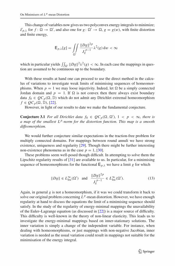
This change of variables now gives us two polyconvex energy integrals to minimize;Ep,λ for f : � → �′, and also one for g : �′ → �, g = g(w), with finite distortionand finite energy,
Ep,λ[g] =∫∫
�′
‖Dg‖2p
J p−1g
λ2(g) dw < ∞
which in particular yields∫∫
�′ ‖Dg‖2λ2(g) < ∞. In each case the mappings in ques-tion are assumed to be continuous up to the boundary.
With these results at hand one can proceed to use the direct method in the calcu-lus of variations to investigate weak limits of minimising sequences of homeomor-phisms. When p = 1 we may loose injectivity. Indeed, let � be a simply connectedJordan domain and p = 1. If � is not convex then there always exist boundarydata f0 ∈ QC p(�, D) which do not admit any Dirichlet extremal homeomorphismf ∈ QC p(�, D), [22].
However, in light of our results to date we make the fundamental conjecture.
Conjecture 3.1 For all Dirichlet data f0 ∈ QC p(�,�′), 1 < p < ∞, there isa map of the smallest L p-norm for the distortion function. This map is a smoothdiffeomorphism.
We would further conjecture similar expectations in the traction-free problem formultiply connected domains. For mappings between round annuli we have strongexistence, uniqueness and regularity [29]. Though there might be further interestingnon-existence phenomena as in the case p = 1, [30].
These problems seem well-posed though difficult. In attempting to solve them theLipschitz regularity results of [31] are available to us. In particular, for a minimisingsequence of homeomorphisms for the functional Ep,λ we have a limit g for which
‖Dg‖ ∈ L∞loc(�
′) and‖Dg‖2p
J p−1g
∈ L∞loc(�
′). (13)
Again, in general g is not a homeomorphism, if it was we could transform it back tosolve our original problem concerning L p-mean distortion. However, we have enoughregularity at hand to discuss the equations the limit of a minimising sequence shouldsatisfy. In the study of the regularity of energy-minimal mappings the unavailabilityof the Euler–Lagrange equation (as discussed in [22]) is a major source of difficulty.This difficulty is well-known in the theory of non-linear elasticity. This leads us toinvestigate the energy-minimal mappings based on inner-stationary solutions. Theinner variation is simply a change of the independent variable. For instance, whendealing with homeomorphisms, or just mappings with non-negative Jacobian, innervariation is needed as the usual variation could result in mappings not suitable for theminimisation of the energy integral.
123
T. Iwaniec et al.
4 The Inner Variation of E p[ f ]
We shall take advantage of the inner variation of the functional
Ep[ f ] =∫∫
�
Kp(z, f ) dz,
for Sobolev homeomorphisms f ∈ W 1,2p
p+1 (�, C) with the smallest L p-mean distor-tion. Since the integrand exhibits 0-homogeneity with respect to the derivatives of fit should come as no surprise that the inner variational equation will involve only theBeltrami coefficient μ = fz̄/ fz . Let us begin with the minimal assumption; that is,when μ is only measurable and |μ(z)| < 1, almost everywhere. Recall from [31] ageneral isotropic energy integral
E[ f ] =∫
�
W (| fz |2, | fz̄ |2), W = W (a, b), a, b � 0.
The inner variation leads to the equation
∂
∂ z̄[(Wa + Wb) fz fz̄] + ∂
∂z[aWa + bWb − W ] = 0
see formula (2.6) in [31]. In our case W = ( a+ba−b
)p = Kp = K(z, f )p, so we have
Wa + Wb = 2p Kp−1/J f and aWa + bWb = 0. Our equation reduces to:
∂
∂ z̄
[2p K
p−1 fz fz̄
J f
]= ∂
∂z[Kp] (14)
which in terms of the Beltrami coefficient reads as
∂
∂ z̄
[2p
(1 + |μ|21 − |μ|2
)p−1μ
1 − |μ|2]
= ∂
∂z
[(1 + |μ|21 − |μ|2
)p]
. (15)
The advantage of using the inner variation, as opposed to the tension equation, lies inthe fact that no regularity of μ is required. In fact, due to its divergence type, the innervariational equation holds in the sense of distributions. It seems reasonable to expectthat the distributional solutions to Eq. (15) are C∞-smooth, but we have no proof ofthis. As evidence to support this conjecture, we assume that μ ∈ W 1,2
loc (�). To dealwith this case we express the Eq. (15), equivalently, as an elliptic system of the form,
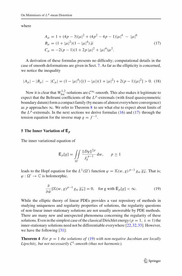
A derivation of these formulas presents no difficulty; computational details in thecase of smooth deformations are given in Sect. 7. As far as the ellipticity is concerned,we notice the inequality
Now it is clear that W 1,2loc -solutions are C∞-smooth. This also makes it legitimate to
expect that the Beltrami coefficients of the L p-extremals (with fixed quasisymmetricboundary datum) form a compact family (by means of almost everywhere convergence)as p approaches ∞. We refer to Theorem 8 to see what else to expect about limits ofthe L p-extremals. In the next sections we derive formulas (16) and (17) through thetension equation for the inverse map g = f −1.
5 The Inner Variation of E p
The inner variational equation of
Ep[g] =∫∫
�′
‖Dg‖2p
J p−1g
dw, p ≥ 1
leads to the Hopf equation for the L1(�′) function ϕ = K(w, g) p−1 gw gw̄. That is;ϕ : �′ → C is holomorphic.
∂
∂w̄[K(w, g)p−1 gw gw̄] = 0, for g with Ep[g] < ∞. (19)
While the elliptic theory of linear PDEs provides a vast repository of methods instudying uniqueness and regularity properties of solutions, the regularity questionsof non-linear inner-stationary solutions are not usually answerable by PDE methods.There are many new and unexpected phenomena concerning the regularity of thesesolutions. Even in the simplest case of the classical Dirichlet energy (p = 1, λ ≡ 1) theinner-stationary solutions need not be differentiable everywhere [22,32,33]. However,we have the following [31]:
Theorem 4 For p = 1 the solutions of (19) with non-negative Jacobian are locallyLipschitz, but not necessarily C1-smooth (thus not harmonic).
123
T. Iwaniec et al.
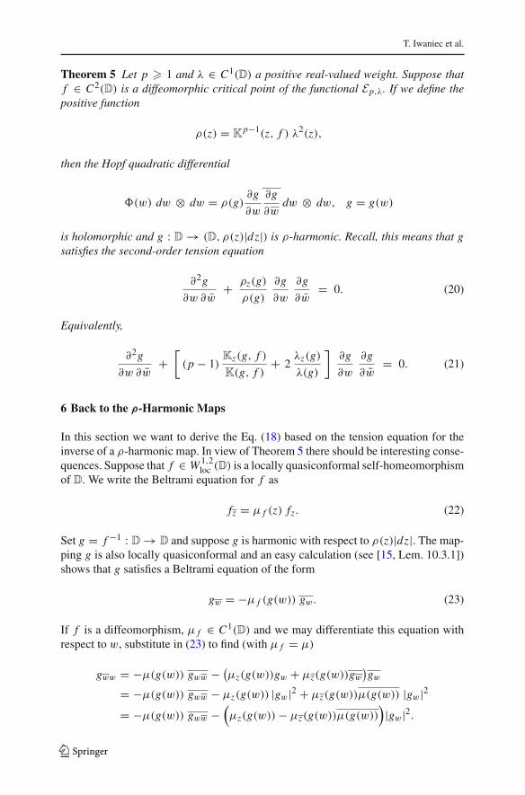
Theorem 5 Let p � 1 and λ ∈ C1(D) a positive real-valued weight. Suppose thatf ∈ C2(D) is a diffeomorphic critical point of the functional Ep,λ. If we define thepositive function
ρ(z) = Kp−1(z, f ) λ2(z),
then the Hopf quadratic differential
(w) dw ⊗ dw = ρ(g)∂g
∂w
∂g
∂wdw ⊗ dw, g = g(w)
is holomorphic and g : D → (D, ρ(z)|dz|) is ρ-harmonic. Recall, this means that gsatisfies the second-order tension equation
∂2g
∂w ∂w̄+ ρz(g)
ρ(g)
∂g
∂w
∂g
∂w̄= 0. (20)
Equivalently,
∂2g
∂w ∂w̄+
[(p − 1)
Kz(g, f )
K(g, f )+ 2
λz(g)
λ(g)
]∂g
∂w
∂g
∂w̄= 0. (21)
6 Back to the ρ-Harmonic Maps
In this section we want to derive the Eq. (18) based on the tension equation for theinverse of a ρ-harmonic map. In view of Theorem 5 there should be interesting conse-quences. Suppose that f ∈ W 1,2
loc (D) is a locally quasiconformal self-homeomorphismof D. We write the Beltrami equation for f as
fz = μ f (z) fz . (22)
Set g = f −1 : D → D and suppose g is harmonic with respect to ρ(z)|dz|. The map-ping g is also locally quasiconformal and an easy calculation (see [15, Lem. 10.3.1])shows that g satisfies a Beltrami equation of the form
gw = −μ f (g(w)) gw. (23)
If f is a diffeomorphism, μ f ∈ C1(D) and we may differentiate this equation withrespect to w, substitute in (23) to find (with μ f = μ)
Since g : D → (D, ρ(z)) is assumed to be harmonic, this means g must satisfy thetension equation
gww + γ (g) gw gw = 0, with γ = (log ρ)z,
and gw �= 0. With (23) this reads as
gww = γ (g) μ(g) |gw|2.
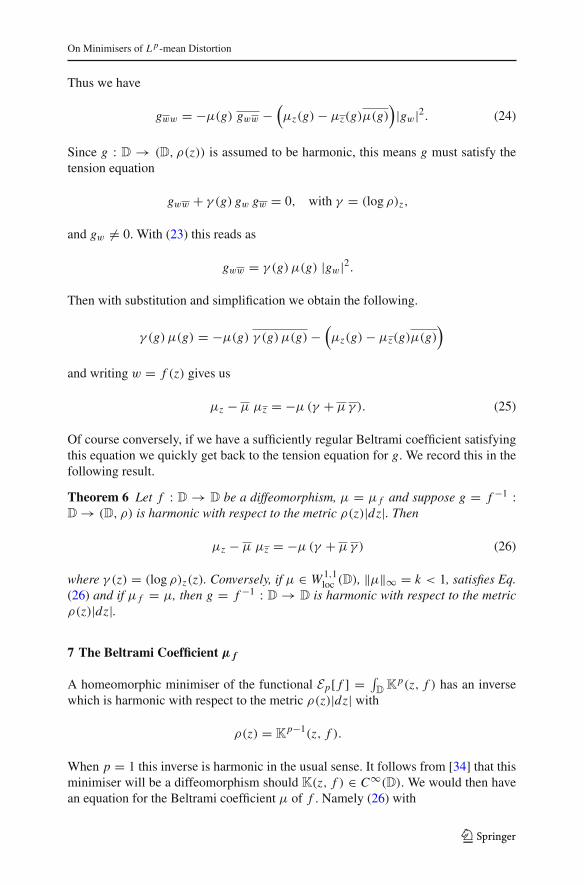
Then with substitution and simplification we obtain the following.
γ (g) μ(g) = −μ(g) γ (g) μ(g) −(μz(g) − μz(g)μ(g)
)
and writing w = f (z) gives us
μz − μ μz = −μ (γ + μ γ ). (25)
Of course conversely, if we have a sufficiently regular Beltrami coefficient satisfyingthis equation we quickly get back to the tension equation for g. We record this in thefollowing result.
Theorem 6 Let f : D → D be a diffeomorphism, μ = μ f and suppose g = f −1 :D → (D, ρ) is harmonic with respect to the metric ρ(z)|dz|. Then
μz − μ μz = −μ (γ + μ γ ) (26)
where γ (z) = (log ρ)z(z). Conversely, if μ ∈ W 1,1loc (D), ‖μ‖∞ = k < 1, satisfies Eq.
(26) and if μ f = μ, then g = f −1 : D → D is harmonic with respect to the metricρ(z)|dz|.
7 The Beltrami Coefficient μ f
A homeomorphic minimiser of the functional Ep[ f ] = ∫D
Kp(z, f ) has an inverse
which is harmonic with respect to the metric ρ(z)|dz| with
ρ(z) = Kp−1(z, f ).
When p = 1 this inverse is harmonic in the usual sense. It follows from [34] that thisminimiser will be a diffeomorphism should K(z, f ) ∈ C∞(D). We would then havean equation for the Beltrami coefficient μ of f . Namely (26) with
123
T. Iwaniec et al.
γ = (p − 1)
(log
1 + |μ|21 − |μ|2
)z= 2(p − 1)
1 − |μ|4 (μzμ + μμz).
Then if we put this formula for γ in (26) we obtain a non-linear equation entirely interms of μ and p.
μz − μ μz = −μ2(p − 1)
1 − |μ|4(μzμ + μμz + μ (μzμ + μμz)
)
= −2(p − 1)
1 − |μ|4(μz |μ|2 + μ2μz + |μ|2 μzμ + μ|μ|2 μz
)
μz
(1 + 2(p − 1)|μ|2
1 − |μ|4)
= μ μz
(1 − 2(p − 1)|μ|2
1 − |μ|4)
− 2(p − 1)μ2
1 − |μ|4 (μz + μ μz).
To simplify we put A = 2(p−1)
1−|μ|4 and consider this equation and its complex conjugateto eliminate μz .
μz
(1 + A|μ|2
)= μ μz
(1 − A|μ|2
)− Aμ2(μz + μ μz)
μz
(1 + A|μ|2
)= μ μz
(1 − A|μ|2
)− Aμ2(μz + μμz).
Thus
μz
(1 + A|μ|2
)2 = μ μz
(1 − A2|μ|4
)− A
(1 + A|μ|2
)μ2 μz
−Aμ|μ|2(
1 + A|μ|2)μz
= μ μz
(1 − A2|μ|4
)− A
(1 + A|μ|2
)μ2 μz
−A|μ|2(μ2 μz
(1 − A|μ|2) − Aμ|μ|2(μz + μμz
)).
Hence, after we collect terms,
[(1 + A|μ|2)2 − A2|μ|6] μz = μ μz − μ2 A
(1 + A|μ|2 + |μ|2 − A|μ|4)μz .
Once we substitute back what A is, and multiply by (1 − |μ|2)(1 + |μ|2)2, we obtain:
[1 + (4p − 3)|μ|2 + (4p2 − 4p − 1)|μ|4 − |μ|6
]μz
=[μ (1 − |μ|2)(1 + |μ|2)2
]μz
−[
2(p − 1)μ2(
1 + 2p |μ|2 + |μ|4) ]
μz (27)
which is the same as (16) and (17), provided μ ∈ C1(D). However, this latter derivationrequires f to be a C2-diffeomorphism. We refer to (27) as the coefficient equation since
123
On Minimisers of L p-mean Distortion
it pertains to the Beltrami coefficient of a smooth minimiser. Notice that if p = 1,then Cμ = 0 in (16) and the coefficient equation reduces to
μz = μ̄μz . (28)
This equation was considered (in this setting) in [2].
7.1 Ellipticity of the Coefficient Equation
We now seek to determine the ellipticity of the coefficient equation (16). We putt = |μ| ∈ [0, 1) and see that
Hence we obtain the following differential inequality.
[1 + |μ| + (2p − 1)|μ|2 + |μ|3
]|μz |
� |μ|[1 + (2p − 1)|μ| + |μ|2 + |μ|3
]|μz |
+[ (
1 + |μ| + (2p − 1)|μ|2 + |μ|3) − (1 − |μ|4) ]
|μz |.
This then gives us
∣∣∣ ∂μ
∂z
∣∣∣ �[
1 − 1 − |μ|41 + |μ| + (2p − 1)|μ|2 + |μ|3
] ∣∣∣ ∂μ
∂ z̄
∣∣∣ �(
1 − 2(1 − |μ|)p + 1
) ∣∣∣ ∂μ
∂ z̄
∣∣∣.
Our standing assumption is that μ is the Beltrami coefficient of a diffeomorphism f :D → D which minimises the functional Ep[ f ] (though of course all these calculationsare purely local). In particular |μ| < 1. Then μ̄ is locally quasiregular. Indeed we seethat if f is K -quasiconformal at a point, then μ f is K ′-quasiregular at that point andK ′ � K + (p − 1)(K − 1). We consequently have the following:
Theorem 7 Let f be a diffeomorphic critical point of Ep and let μ = μ f be itsBeltrami coefficient. Then μ̄ is a locally quasiregular mapping.
Since quasiregular mappings are discrete and open we have the following corollarystating that distortion satisfies a strong maximum principle.
123
T. Iwaniec et al.
Corollary 3 Let f be a diffeomorphic critical point of Ep, 1 < p < ∞. Let U � D
be compact and z0 ∈ U. Then
K(z0, f ) < maxz∈∂U
K(z, f )
unless K(z, f ) is constant.
We also make the following observation.
Corollary 4 Let f : D → D be a diffeomorphic L p-extremal for Ep with some1 � p < ∞. If |μ f | is constant then the complex coefficient μ f , being locallyquasiregular, is constant as well.
Corollary 1 shows the case when the L p-minimiser has constant distortion; thereare many more such examples.
The coefficient equation is quite interesting in and of itself. Notice that the coef-ficients Aμ, Bμ and Cμ are real analytic functions in {μ : |μ| < 1}. Thus Cauchy–Kovalevsky theory can be applied to the quasilinear equation (27)—we will discussthis elsewhere. We would also like to point out the following non-rigorous observa-tions (which are discussed more carefully in [27]) about the behaviour as p → ∞.Suppose we fix a quasisymmetric boundary datum f0 : D → D and suppose for eachp the minimiser of Ep exists, is a diffeomorphism and has Beltrami coefficient μ(p).Dividing by 4p2 and letting p → ∞ one notices that should μ = lim p→∞ μ(p) exist,then the coefficient equation would, in the limit, becomes
μz |μ|4 = −μ2 μz |μ|2.
This, when simplified, reads as (|μ|2)z = 0 and hence |μ| ≡ const. This suggeststhat as p → ∞ the distortion of the L p-extremals should converge in some sense toa constant. A question then to consider is whether or not the limiting mapping (whichalways exists in the sense of weak convergence in W 1,s , 1 � s < 2) is an extremalquasiconformal mapping.
In fact it is not too difficult to prove the following interesting theorem.
Theorem 8 Let f0 : Donto−→D be a given K -quasiconformal mapping (serving as bound-
ary data). Consider a sequence { f j } ⊂ QC p j (D, D) of L p j -extremals f j : Donto−→D
under the boundary constraint f j = f0 : Sonto−→S, whose Beltrami coefficients μ j
converge almost everywhere to μ as 1 < p j → ∞. Then
• |μ(z)| � K−1K+1 , almost everywhere.
• There is a subsequence, again denoted by { f j }, such that f j ⇀ f, weakly inW 1,s(D) , forall1 � s < 2.
• f ∈ W 1,2(D).• The limit map is quasiconformal and satisfies the Beltrami equation
fz̄ = μ(z) fz . (29)
123
On Minimisers of L p-mean Distortion
• f is an extremal quasiconformal mapping for the boundary values f0.
To conclude we make some final observations.
• Obviously, any sequence {μ j } with |μ j (z)| � k(z) < 1 almost everywhere, containsa subsequence converging weakly to a measurable function μ with |μ(z)| � k(z) <
1. However, when passing to the weak limit (precisely, G-limit) of the Beltramiequations f j
z̄ = μ j (z) f jz we may not arrive at fz̄ = μ(z) fz . The interested reader
is referred to [35] for the related issues of G-compactness of the Beltrami operators,see Example 8.1 therein. Nevertheless, because of ellipticity of the Eq. (16), it seemsthat weak convergence of the distributional solutions μ j would actually yield almosteverywhere convergence.
• The L1-normalization of the holomorphic Hopf differentials
j (w) dw ⊗ dw, j (w) = Kp j −1j (w) g j
w g jw,
where K j (w) = K(z, f j ) and z = g j (w) associated with g j = ( f j )−1 wouldform a Hamilton sequence for the extremal quasiconformal mapping g = f −1.
Of course what we really want in Theorem 8 is to remove any hypotheses at all onthe convergence (weak, almost everywhere or otherwise).
References
1. Iwaniec, T., Šverák, V.: On mappings with integrable dilatation. Proc. Am. Math. Soc. 118(1), 181–188(1993)
2. Astala, K., Iwaniec, T., Martin, G.J.: Bilipschitz homeomorphisms of the circle and nonlinear Beltramiequations. Quad. Mate. 23, 105–117 (2009)
3. Astala, K., Iwaniec, T., Martin, G.J., Onninen, J.: Extremal mappings of finite distortion. Proc. Lond.Math. Soc. 91, 655–702 (2005)
4. Duren, P.: Harmonic Mappings Between Planar Domains. Cambridge University Press, Cambridge(2004)
5. Hussan, J., Martin, G.: Fully non-linear models for the deformation of cellular structures. J. Mod.Math. Front. 2, 51–64 (2013)
6. Hussan, J., Martin, G., McKubre-Jordens, M.: New approaches to modeling elastic media. In: MaterialsScience, Chap. 18, pp. 465– 485 (2013) (ISBN 980-953-307-918-4)
7. Beurling, A., Ahlfors, L.V.: The boundary correspondence under quasiconformal mappings. Acta Math.96, 125–142 (1956)
8. Nag, S.: Canadian Mathematical Society Monographs. The complex analytic theory of Teichmüllerspaces. Wiley, New York (1988)
9. Teichmüller, O.: Gesammelte Abhandlungen (edited and with a preface by Lars V. Ahlfors and Fred-erick W. Gehring). Springer-Verlag, Berlin (1982)
11. Yao, G.: Is there always an extremal Teichmüller mapping? J. Anal. Math. 94, 363–375 (2004)12. Strebel, K.: Is there always a unique extremal Teichmüller mapping. Proc. Am. Math. Soc. 90, 240–242
(1984)13. Reich, E., Strebel, K.: Extremal quasiconformal mappings with given boundary values. In: Ahlfors, L.,
et al. (eds.) Contributions to Analysis. Academic Press, New York, pp. 375–392 (1974) (a collectionof papers dedicated to Lipman Bers)
14. Strebel, K.: Ergebnisse der Mathematik und ihrer Grenzgebiete (3). Quadratic differentials, 5th edn.Springer-Verlag, Berlin (1984)
123
T. Iwaniec et al.
15. Astala, K., Iwaniec, T., Martin, G.J.: Princeton Mathematical Series. Elliptic partial differential equa-tions and quasiconformal mappings in the plane, 48th edn. Princeton University Press, Princeton (2009)
16. Pavlovich, M.: Boundary correspondence under harmonic quasiconformal homeomorphisms of theunit disk. Ann. Acad. Sci. Fenn. Math. 27, 365–372 (2002)
17. Iwaniec, T., Onninen, J.: Invertibility versus Lagrange equation for traction free energy-minimal defor-mations (2013, preprint)
18. Jost, J.: Harmonic maps between surfaces. In: Lecture Notes in Mathematics, vol. 1062. Springer-Verlag, Berlin (1984)
19. Schoen, R., Yau, S.T.: On univalent harmonic maps between surfaces. Invent. Math. 44, 265–278(1978)
20. Cheng, S.Y., Yau, S.T.: Differential equations on Riemannian manifolds and their geometric applica-tions. Commun. Pure Appl. Math. 28, 333–354 (1975)
21. Li, P., Tam, L.-F.: Uniqueness and regularity of proper harmonic maps. Ann. Math. 137, 167–201(1993)
22. Iwaniec, T., Onninen, J.: Mappings of least Dirichlet energy and their Hopf differentials. Arch. Ration.Mech. Anal. 209, 401–453 (2013)
23. Wolf, M.: The Teichmüller theory of harmonic maps. J. Differ. Geom. 29, 449–479 (1989)24. Wan, T.Y.H.: Constant mean curvature surface, harmonic maps and universal Teichmüller space. J.
Diff. Geom. 35, 643–657 (1992)25. Morrey, C.B.: Quasi-convexity and the lower semicontinuity of multiple integrals. Pac. J. Math. 2,
25–53 (1952)26. Iwaniec, T., Martin, G.: Oxford Mathematical Monographs. Geometric function theory and non-linear
analysis. The Clarendon Press, Oxford University Press, New York (2001)27. Iwaniec, T., Martin, G., Onninen, J.: Mappings of smallest L p-mean distortion (2014, in progress)28. Hencl, S., Koskela, P.: Regularity of the inverse of a planar Sobolev homeomorphism. Arch. Ration.
Mech. Anal. 180(1), 75–95 (2006)29. Martin, G.J., McKubre-Jordens, M.: Deformations with smallest weighted L p average distortion and
Nitsche-type phenomena. J. Lond. Math. Soc. 85, 282–300 (2012)30. Martin, G.J.: The Teichmüller problem for mean distortion. Ann. Acad. Sci. Fenn. 34, 1–15 (2009)31. Iwaniec, T., Kovalev, L.V., Onninen, J.: Lipschitz regularity for inner variational equations. Duke Math.
J. 162(4), 643–672 (2013)32. Cristina, J., Iwaniec, T., Kovalev, L.V., Onninen, J.: The Hopf–Laplace equation: harmonicity and
regularity. Ann. Sc. Norm. Sup. Pisa Cl. Sci. (2014, to appear)33. Iwaniec, T., Kovalev, L.V., Onninen, J.: Hopf differentials and smoothing Sobolev homeomorphisms.
(arXiv:1310.4872)35. Giannetti, F., Iwaniec, T., Kovalev, L.V., Moscariello, G., Sbordone, C.: On G-compactness of the
Beltrami operators. In: Nonlinear Homogenization and its Applications to Composites, Polycrystalsand Smart Materials. Kluwert Academic Publishers, The Netherlands, pp. 107–138 (2004)