On multigrid-CG for efficient topology optimization

Oded Amir1, Niels Aage2 and Boyan S. Lazarov21 Faculty of Civil and Environmental Engineering, Technion - Israel Institute of Technology

2 Department of Mechanical Engineering, Technical University of Denmark

1 Abstract

This article presents a computational approach that facilitates the efficient solution of 3-D struc-tural topology optimization problems on a standard PC. Computing time associated with solvingthe nested analysis problem is reduced significantly in comparison to other existing approaches.The cost reduction is obtained by exploiting specific characteristics of a multigrid preconditionedconjugate gradients (MGCG) solver. In particular, the number of MGCG iterations is reduced byrelating it to the geometric parameters of the problem. At the same time, accurate outcome of theoptimization process is ensured by linking the required accuracy of the design sensitivities to theprogress of optimization. The applicability of the proposed procedure is demonstrated on several2-D and 3-D examples involving up to hundreds of thousands of degrees of freedom. Implementedin MATLAB, the MGCG-based program solves 3-D topology optimization problems in a matterof minutes. This paves the way for efficient implementations in computational environments thatdo not enjoy the benefits of high performance computing, such as applications on mobile devicesand plug-ins for modeling software.

Keywords: Topology optimization, preconditioned conjugate gradients, multigrid.

2 Introduction

In typical structural topology optimization procedures, the computational effort involved in re-peated solution of the analysis equations dominates the computational cost of the whole process.This motivates the search for efficient approaches aimed at reducing the computational effortinvested in the analysis. The current contribution aims primarily at deriving computational proce-dures for performing 3-D topology optimization on a standard PC within high-level programmingenvironments such as MATLAB. To ensure that the approach can be easily ported to other pro-gramming environments, the suggested code is based almost entirely on the SuiteSparse library [18].This general approach paves the way for integrating 3-D topology optimization in CAD software,e.g. within the Grasshopper-Rhino TopOpt component released recently; as well as in applicationsfor mobile devices such as the TopOpt app [2]. Even though large-scale parallel procedures are notof primary concern in this work, the general form of the iterative solver presented here is indeedalso applicable to large-scale topology optimization problems.

Reduction of computational effort in topology optimization has been approached from variousstandpoints over the past few years. One of the major research trajectories examines the applicationof multiple computational scales and resolutions, thus avoiding the inherent high cost of solvingsequences of finite element analyses on a fine mesh. Kim and Yoon [25] suggested the conceptof multi-resolution multi-scale topology optimization (MTOP) where optimization is performedwhile progressively refining the grid. They used a wavelet-based parametrization of the densitydistribution, as was also suggested by Poulsen [30] in the context of regularizing topological design.The utilization of wavelet bases was later extended by Kim et al. [23] who applied adaptive wavelet-Galerkin analysis to multi-scale topology optimization. Stainko [35] proposed a multilevel schemewhere optimization is first performed on a coarse grid, which is then adaptively refined in theinterface between solid and void. Ultimately, a fine-resolution design is achieved for a relativelylow computational expense. Using this strategy, it is not clear whether fine features that did notexist in the coarse design can emerge in the finer levels. More recently, another multi-resolution

1

topology optimization scheme was suggested, where the density distribution is realized on a finerscale than the displacements [28, 29].

Other approaches for saving computational cost include reducing the number of design variablesby using adaptive design variable fields [21]; generating sets of Pareto-optimal topologies within asingle optimization process [37]; and adaptive reduction of the number of design variables based onthe history of each variable during optimization [24]. However, the current study is mostly relatedto contributions focusing solely on reducing the cost involved in repeated solution of the nestedanalysis equations, either by recycling of Krylov subspaces [42]; integrating approximate reanalysis[4, 13, 44, 6]; and truncating iterative solutions [5, 3].

It was observed in some of the recent investigations that accurate results of the optimizationprocess can be achieved even if the analysis equations are not solved to full accuracy [e.g. 42, 5, 3].This observation is based primarily on numerical experimentation and providing comprehensivemathematical argumentation is still a challenge for future research. Results presented here demon-strate again that approximate solution of the analysis equations can yield accurate outcome of theoptimization. Several advancements with respect to previous studies are presented, that result insignificant reduction in computational effort. We continue to use the framework of Krylov sub-space iterative solvers, particularly the Preconditioned Conjugate Gradients method (PCG), butwith a multigrid V-cycle applied as a preconditioner. The resulting procedure, typically termedMGCG (MultiGrid Conjugate Gradients) is nowadays a well-established technique and was shownto provide mesh-independent convergence as well as good parallel scalability [39, 8].

This article focuses on the effective utilization of MGCG for the purpose of solving the nestedanalysis equations arising in topology optimization problems, a topic which has yet to be explored.It is shown that straightforward implementation of MGCG indeed leads to better performancecompared to other preconditioning techniques. More importantly, further reduction in computa-tional cost is possible by exploiting specific characteristics of MGCG and by linking the accuracyof the MGCG analysis to the progress of optimization. We show that MGCG is unique due tothe relations between the required number of iterations and the geometric parameters of the prob-lem - namely the number of grid levels and the filter size. Furthermore, we propose to relate thetolerance of the iterative solution of the analysis equations to the progress of optimization. Thismeans that the analysis is solved to full accuracy only when the optimization problem approachesa solution, whereas approximations are sufficient in earlier stages as long as they do not hamperthe progress towards an optimum. In other words, a ‘semi-nested’ approach is taken: The analysisis indeed solved separately from the optimization but the effort invested in it, and consequentlythe accuracy achieved, are both linked to the progress of optimization.

Up to date, we are not aware of any publications concerning the utilization of MGCG for solv-ing the analysis equations arising in topology optimization problems. This might be related tothe expected difficulty of multigrid methods to deal with high contrast in coefficients - an inher-ent property due to the desired solid-void (or 1-0) density distribution. Nevertheless, multigridsolvers were proposed for solving the complete Karush-Kuhn-Tucker (KKT) system of equationscorresponding to topology optimization problems [27, 36]. Another application arises when follow-ing the phase field approach to topology optimization, where a multigrid method was utilized forsolving the Cahn-Hilliard equations [43].

Another alternative for improving the solution timing is the employment of parallel computingfor solving both the state problem as well as the optimization [1]. Such a parallelization approachleads to very high parallel efficiency, i.e., good utilization of a large-scale parallel computer. How-ever, good scalability is irrelevant if the solution method is very slow. Our main interest is indecreasing the total time for a given set of computational resources. Therefore, multigrid solversare excellent candidates as they are parallelizable and numerically scalable, i.e., the solution timeis proportional to the problem size. Outline of the main challenges for multigrid parallelizationcan be found in [17] and recent reports on solving very large-scale problems on one of the fastestsupercomputers can be found in [9, 10]. In the current study, the main focus is on demonstratingand discussing the applicability of MGCG as a solver of the linear analysis equations in topologyoptimization. Reporting the challenges of parallel implementation is left for future work.

The article is organized as follows. The optimization problem formulation and standard im-plementation of the multigrid-CG procedure are briefly discussed in Section 3. The heart of thearticle is in Section 4, where observations based on numerical experimentation and the suggestedapproximate approach are presented. This is followed by several examples involving 3-D optimizeddesigns in Section 5. Finally, discussion and conclusions are given in Section 6.

2

3 Problem formulation and computational framework

For demonstrative purposes we address classical problems in structural topology optimizationinvolving linear elasticity, namely minimum compliance and force inverter problems. These arehereby reviewed briefly for the sake of completeness. We follow the density-based approach [11]and apply the modified SIMP interpolation scheme relating density to elastic stiffness [34]. Thisdoes not imply any loss of generality - various topology optimization approaches share the samebasic formulation and can equally benefit from the advancements discussed in this article. Theconsidered optimization problem has the following generic form

minρφ(ρ) = lTu

s.t.:

N∑e=1

veρe ≤ V

0 ≤ ρe ≤ 1 e = 1, ..., N

with: K(ρ)u = f (1)

where ρ represents the density distribution; K(ρ) is the stiffness matrix; f is the load vector; u isthe displacements vector; ve is the element volume; and V is the total available volume. In eachfinite element the elastic stiffness is given by the modified SIMP interpolation rule

E(ρ) = Emin + (Emax − Emin)ρp

where Emax is typically 1; Emin is a small number; and the penalty power p is typically set to 3.The ratio between Emax and Emin will be referred to later as the contrast of the layout because itcontrols the sharpness of the stiffness distribution for a given 0-1 topological layout.

Minimum compliance optimization is obtained by setting l ≡ f while for the force inverterproblem l is a vector with the value of 1 at the output degree of freedom and zeros otherwise.Design sensitivities are computed by the adjoint method. For both cases, the sensitivity of theobjective with respect to a particular element density is given by

∂φ

∂ρe= −uT ∂K

∂ρeu

where K(ρ)u = l, thus for the compliance problem u ≡ u. Using the computed gradients of theobjective and the constraint, the problem can be solved by various means. We apply either anoptimality criteria (OC) procedure or a first-order nonlinear programming method - MMA [38].Mesh-independence and regularization are treated by either sensitivity filtering [32, 33] or densityfiltering [16, 14].

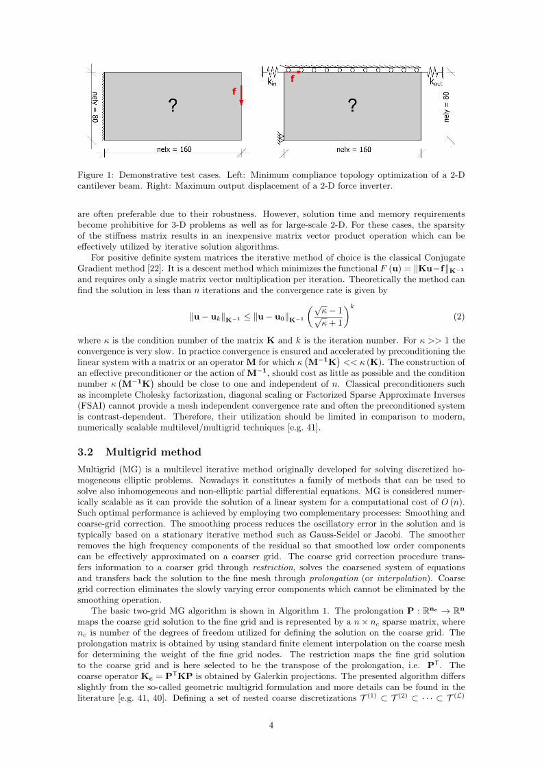
For demonstrating the performance of MGCG-based procedures we utilize three test cases: 1)Minimum compliance topology optimization of a beam with a point load, typically referred to asthe MBB-beam, with various mesh resolutions; 2) Minimum compliance topology optimization ofa cantilever beam, with a single point load at the middle of the free face; and 3) Maximum outputdisplacement of a force inverter, see Figure 1. For the cantilever beam, The FE mesh resolutionis 160×80; the volume fraction is 0.4; and the modified SIMP penalty is 3.0. The same mesh andpenalty are used also for the force inverter, but with a volume fraction of 0.3. Within the multigridV-cycle, we apply a single damped Jacobi smoothening cycle with ω = 0.8. We use up to fourmultigrid levels: According to the specified number of levels, a direct solve is performed on either80×40, 40×20 or 20×10 grid. With 3-D applications in mind, it is clear that the coarsest levelshould be chosen such that a direct solve can be performed efficiently.

3.1 Preconditioned Conjugate Gradient method

The focus here is on the effective solution of the linear system of equations Ku = f arising from afinite element discretization of the state problem. The stiffness matrix is large, sparse and positivedefinite. The solution u can be obtained using either direct methods [e.g. 18] or iterative methods[31]. For full matrices, the computational cost of direct Cholesky decomposition is of O

(n3), while

for sparse matrices direct methods such as nested dissection require O(n3/2

)operations, where

n is the size of the stiffness matrix [18]. For small problems, particularly in 2-D, direct solvers

3

Figure 1: Demonstrative test cases. Left: Minimum compliance topology optimization of a 2-Dcantilever beam. Right: Maximum output displacement of a 2-D force inverter.

are often preferable due to their robustness. However, solution time and memory requirementsbecome prohibitive for 3-D problems as well as for large-scale 2-D. For these cases, the sparsityof the stiffness matrix results in an inexpensive matrix vector product operation which can beeffectively utilized by iterative solution algorithms.

For positive definite system matrices the iterative method of choice is the classical ConjugateGradient method [22]. It is a descent method which minimizes the functional F (u) = ‖Ku−f‖K−1

and requires only a single matrix vector multiplication per iteration. Theoretically the method canfind the solution in less than n iterations and the convergence rate is given by

‖u− uk‖K−1 ≤ ‖u− u0‖K−1

(√κ− 1√κ+ 1

)k(2)

where κ is the condition number of the matrix K and k is the iteration number. For κ >> 1 theconvergence is very slow. In practice convergence is ensured and accelerated by preconditioning thelinear system with a matrix or an operator M for which κ

(M−1K

)<< κ (K). The construction of

an effective preconditioner or the action of M−1, should cost as little as possible and the conditionnumber κ

(M−1K

)should be close to one and independent of n. Classical preconditioners such

as incomplete Cholesky factorization, diagonal scaling or Factorized Sparse Approximate Inverses(FSAI) cannot provide a mesh independent convergence rate and often the preconditioned systemis contrast-dependent. Therefore, their utilization should be limited in comparison to modern,numerically scalable multilevel/multigrid techniques [e.g. 41].

3.2 Multigrid method

Multigrid (MG) is a multilevel iterative method originally developed for solving discretized ho-mogeneous elliptic problems. Nowadays it constitutes a family of methods that can be used tosolve also inhomogeneous and non-elliptic partial differential equations. MG is considered numer-ically scalable as it can provide the solution of a linear system for a computational cost of O (n).Such optimal performance is achieved by employing two complementary processes: Smoothing andcoarse-grid correction. The smoothing process reduces the oscillatory error in the solution and istypically based on a stationary iterative method such as Gauss-Seidel or Jacobi. The smootherremoves the high frequency components of the residual so that smoothed low order componentscan be effectively approximated on a coarser grid. The coarse grid correction procedure trans-fers information to a coarser grid through restriction, solves the coarsened system of equationsand transfers back the solution to the fine mesh through prolongation (or interpolation). Coarsegrid correction eliminates the slowly varying error components which cannot be eliminated by thesmoothing operation.

The basic two-grid MG algorithm is shown in Algorithm 1. The prolongation P : Rnc → Rn

maps the coarse grid solution to the fine grid and is represented by a n× nc sparse matrix, wherenc is number of the degrees of freedom utilized for defining the solution on the coarse grid. Theprolongation matrix is obtained by using standard finite element interpolation on the coarse meshfor determining the weight of the fine grid nodes. The restriction maps the fine grid solutionto the coarse grid and is here selected to be the transpose of the prolongation, i.e. PT. Thecoarse operator Kc = PTKP is obtained by Galerkin projections. The presented algorithm differsslightly from the so-called geometric multigrid formulation and more details can be found in theliterature [e.g. 41, 40]. Defining a set of nested coarse discretizations T (1) ⊂ T (2) ⊂ · · · ⊂ T (L)

4

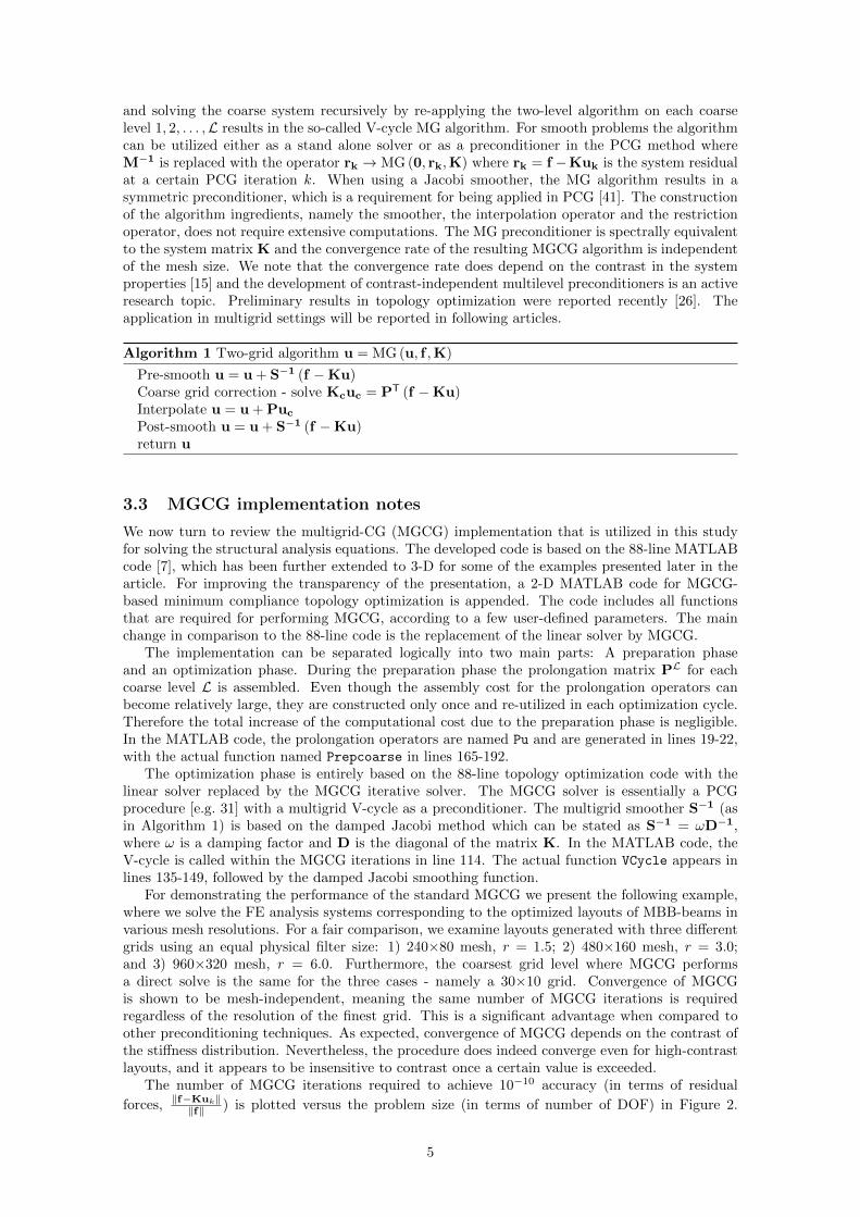
and solving the coarse system recursively by re-applying the two-level algorithm on each coarselevel 1, 2, . . . ,L results in the so-called V-cycle MG algorithm. For smooth problems the algorithmcan be utilized either as a stand alone solver or as a preconditioner in the PCG method whereM−1 is replaced with the operator rk → MG (0, rk,K) where rk = f −Kuk is the system residualat a certain PCG iteration k. When using a Jacobi smoother, the MG algorithm results in asymmetric preconditioner, which is a requirement for being applied in PCG [41]. The constructionof the algorithm ingredients, namely the smoother, the interpolation operator and the restrictionoperator, does not require extensive computations. The MG preconditioner is spectrally equivalentto the system matrix K and the convergence rate of the resulting MGCG algorithm is independentof the mesh size. We note that the convergence rate does depend on the contrast in the systemproperties [15] and the development of contrast-independent multilevel preconditioners is an activeresearch topic. Preliminary results in topology optimization were reported recently [26]. Theapplication in multigrid settings will be reported in following articles.

Algorithm 1 Two-grid algorithm u = MG (u, f ,K)

Pre-smooth u = u + S−1 (f −Ku)Coarse grid correction - solve Kcuc = PT (f −Ku)Interpolate u = u + Puc

Post-smooth u = u + S−1 (f −Ku)return u

3.3 MGCG implementation notes

We now turn to review the multigrid-CG (MGCG) implementation that is utilized in this studyfor solving the structural analysis equations. The developed code is based on the 88-line MATLABcode [7], which has been further extended to 3-D for some of the examples presented later in thearticle. For improving the transparency of the presentation, a 2-D MATLAB code for MGCG-based minimum compliance topology optimization is appended. The code includes all functionsthat are required for performing MGCG, according to a few user-defined parameters. The mainchange in comparison to the 88-line code is the replacement of the linear solver by MGCG.

The implementation can be separated logically into two main parts: A preparation phaseand an optimization phase. During the preparation phase the prolongation matrix PL for eachcoarse level L is assembled. Even though the assembly cost for the prolongation operators canbecome relatively large, they are constructed only once and re-utilized in each optimization cycle.Therefore the total increase of the computational cost due to the preparation phase is negligible.In the MATLAB code, the prolongation operators are named Pu and are generated in lines 19-22,with the actual function named Prepcoarse in lines 165-192.

The optimization phase is entirely based on the 88-line topology optimization code with thelinear solver replaced by the MGCG iterative solver. The MGCG solver is essentially a PCGprocedure [e.g. 31] with a multigrid V-cycle as a preconditioner. The multigrid smoother S−1 (asin Algorithm 1) is based on the damped Jacobi method which can be stated as S−1 = ωD−1,where ω is a damping factor and D is the diagonal of the matrix K. In the MATLAB code, theV-cycle is called within the MGCG iterations in line 114. The actual function VCycle appears inlines 135-149, followed by the damped Jacobi smoothing function.

For demonstrating the performance of the standard MGCG we present the following example,where we solve the FE analysis systems corresponding to the optimized layouts of MBB-beams invarious mesh resolutions. For a fair comparison, we examine layouts generated with three differentgrids using an equal physical filter size: 1) 240×80 mesh, r = 1.5; 2) 480×160 mesh, r = 3.0;and 3) 960×320 mesh, r = 6.0. Furthermore, the coarsest grid level where MGCG performsa direct solve is the same for the three cases - namely a 30×10 grid. Convergence of MGCGis shown to be mesh-independent, meaning the same number of MGCG iterations is requiredregardless of the resolution of the finest grid. This is a significant advantage when compared toother preconditioning techniques. As expected, convergence of MGCG depends on the contrast ofthe stiffness distribution. Nevertheless, the procedure does indeed converge even for high-contrastlayouts, and it appears to be insensitive to contrast once a certain value is exceeded.

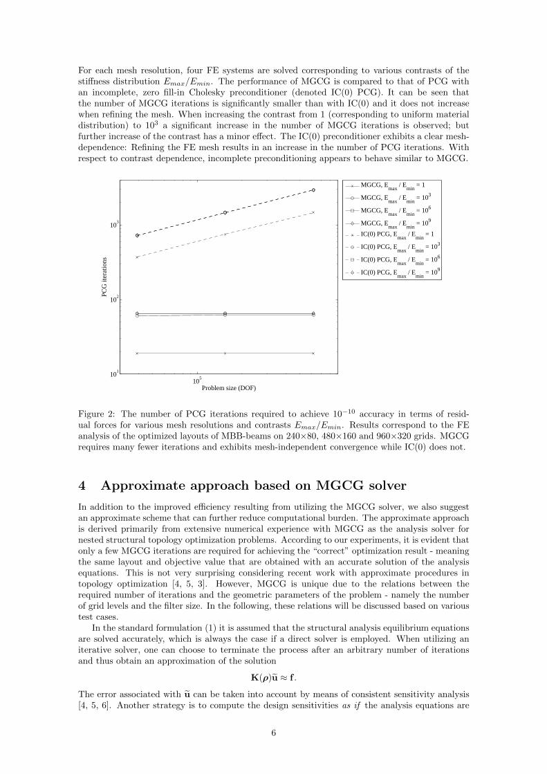
The number of MGCG iterations required to achieve 10−10 accuracy (in terms of residual

forces, ‖f−Kuk‖‖f‖ ) is plotted versus the problem size (in terms of number of DOF) in Figure 2.

5

For each mesh resolution, four FE systems are solved corresponding to various contrasts of thestiffness distribution Emax/Emin. The performance of MGCG is compared to that of PCG withan incomplete, zero fill-in Cholesky preconditioner (denoted IC(0) PCG). It can be seen thatthe number of MGCG iterations is significantly smaller than with IC(0) and it does not increasewhen refining the mesh. When increasing the contrast from 1 (corresponding to uniform materialdistribution) to 103 a significant increase in the number of MGCG iterations is observed; butfurther increase of the contrast has a minor effect. The IC(0) preconditioner exhibits a clear mesh-dependence: Refining the FE mesh results in an increase in the number of PCG iterations. Withrespect to contrast dependence, incomplete preconditioning appears to behave similar to MGCG.

105

101

102

103

Problem size (DOF)

PCG

iter

atio

ns

MGCG, E

max / E

min = 1

MGCG, Emax

/ Emin

= 103

MGCG, Emax

/ Emin

= 106

MGCG, Emax

/ Emin

= 109

IC(0) PCG, Emax

/ Emin

= 1

IC(0) PCG, Emax

/ Emin

= 103

IC(0) PCG, Emax

/ Emin

= 106

IC(0) PCG, Emax

/ Emin

= 109

Figure 2: The number of PCG iterations required to achieve 10−10 accuracy in terms of resid-ual forces for various mesh resolutions and contrasts Emax/Emin. Results correspond to the FEanalysis of the optimized layouts of MBB-beams on 240×80, 480×160 and 960×320 grids. MGCGrequires many fewer iterations and exhibits mesh-independent convergence while IC(0) does not.

4 Approximate approach based on MGCG solver

In addition to the improved efficiency resulting from utilizing the MGCG solver, we also suggestan approximate scheme that can further reduce computational burden. The approximate approachis derived primarily from extensive numerical experience with MGCG as the analysis solver fornested structural topology optimization problems. According to our experiments, it is evident thatonly a few MGCG iterations are required for achieving the “correct” optimization result - meaningthe same layout and objective value that are obtained with an accurate solution of the analysisequations. This is not very surprising considering recent work with approximate procedures intopology optimization [4, 5, 3]. However, MGCG is unique due to the relations between therequired number of iterations and the geometric parameters of the problem - namely the numberof grid levels and the filter size. In the following, these relations will be discussed based on varioustest cases.

In the standard formulation (1) it is assumed that the structural analysis equilibrium equationsare solved accurately, which is always the case if a direct solver is employed. When utilizing aniterative solver, one can choose to terminate the process after an arbitrary number of iterationsand thus obtain an approximation of the solution

K(ρ)u ≈ f .

The error associated with u can be taken into account by means of consistent sensitivity analysis[4, 5, 6]. Another strategy is to compute the design sensitivities as if the analysis equations are

6

solved accurately, meaning that the error is transferred further to the design sensitivities

∂φ

∂ρe≈ −u

T ∂K

∂ρeu (3)

where u is an approximation of the adjoint vector u, obtained by an iterative solver in the samemanner as u. According to recent experience, this strategy tends to yield better optimized perfor-mance than the consistent sensitivity approach [6].

With the goal of formulating an efficient yet reliable approximate procedure, two central re-quirements are considered: 1) A minimum number of MGCG iterations should be imposed, withrelation to the geometric parameters of the problem - the number of grid levels and the filter size;and 2) The stopping criterion for MGCG should be related to the progress of optimization in orderto avoid local minima. These two aspects are addressed in the following.

4.1 Imposing a minimum number of MGCG iterations

A minimum number of MGCG iterations is imposed, essentially in order to ensure reasonableerror reduction throughout the fine mesh. In its basic (non-preconditioned) form, the error inCG propagates through a single finite element in every iteration. For this reason, “long” domainsare less preferable than equilateral domains - computing an accurate solution will require moreiterations the further the error needs to “travel”. In the context of multigrid, one would requirethat the error propagates throughout the fine grid, while the solution (the preconditioning step)on the coarsest grid level is assumed to be accurate. The introduction of a filter improves thissituation, because the filter operation has a smoothening effect on all fine grid points within thefiltered domain. Therefore, a heuristic rule for a minimum number of MGCG iterations will ensurethat the error is propagated by MGCG from the coarse grid points into the filtered domain.

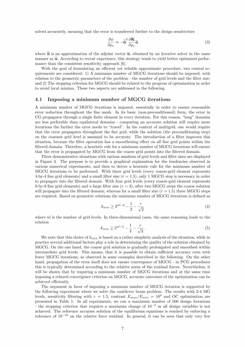
Three demonstrative situations with various numbers of grid levels and filter sizes are displayedin Figure 3. The purpose is to provide a graphical explanation for the tendencies observed invarious numerical experiments, and then to derive a heuristic rule for the minimum number ofMGCG iterations to be performed. With three grid levels (every coarse-grid element represents4-by-4 fine grid elements) and a small filter size (r = 1.5), only 1 MGCG step is necessary in orderto propagate into the filtered domain. With four grid levels (every coarse-grid element represents8-by-8 fine grid elements) and a large filter size (r = 3), after two MGCG steps the coarse solutionwill propagate into the filtered domain; whereas for a small filter size (r = 1.5) three MGCG stepsare required. Based on geometric relations the minimum number of MGCG iterations is defined as

kmin ≥ 2nl−2 − 1

2− r√

2(4)

where nl is the number of grid levels. In three-dimensional cases, the same reasoning leads to therelation

kmin ≥ 2nl−2 − 1

2− r√

3. (5)

We note that this choice of kmin is based on a rather simplistic analysis of the situation, while inpractice several additional factors play a role in determining the quality of the solution obtained byMGCG. On the one hand, the coarse grid solution is gradually prolongated and smoothed withinintermediate grid levels. This means, that it is possible to obtain sufficient accuracy even withfewer MGCG iterations, as observed in some examples described in the following. On the otherhand, propagation of the error itself does not ensure convergence of MGCG - in PCG proceduresthis is typically determined according to the relative norm of the residual forces. Nevertheless, itwill be shown that by requiring a minimum number of MGCG iterations and at the same timeimposing a relaxed convergence criterion on MGCG, accurate outcomes of the optimization can beachieved efficiently.

The argument in favor of imposing a minimum number of MGCG iteration is supported bythe following experiment where we solve the cantilever beam problem. The results with 2-4 MGlevels, sensitivity filtering with r = 1.5, contrast Emax/Emin = 109 and OC optimization arepresented in Table 1. In all experiments, we run a maximum number of 500 design iterations- the stopping criterion that requires a maximum change of 10−3 in all design variables is notachieved. The reference accurate solution of the equilibrium equations is reached by enforcing atolerance of 10−10 on the relative force residual. In general, it can be seen that only very few

7

Figure 3: The effect of the number of grid levels and filter size on the number of MGCG iterationsperformed until the coarse-grid solution initially propagates into the filtered domain. Left: 3 gridlevels, r = 1.5, 1 iteration; middle: 4 grid levels, r = 3, 2 iterations; right: 4 grid levels, r = 1.5, 3iterations.

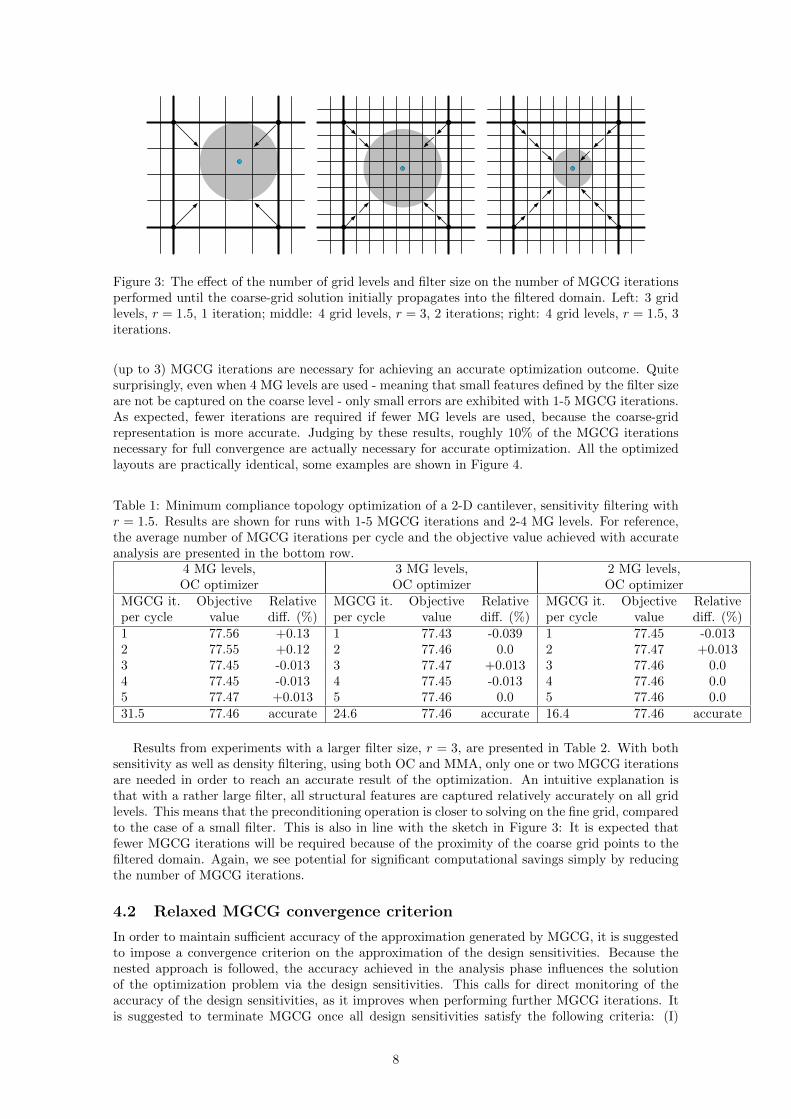
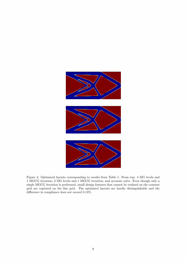
(up to 3) MGCG iterations are necessary for achieving an accurate optimization outcome. Quitesurprisingly, even when 4 MG levels are used - meaning that small features defined by the filter sizeare not be captured on the coarse level - only small errors are exhibited with 1-5 MGCG iterations.As expected, fewer iterations are required if fewer MG levels are used, because the coarse-gridrepresentation is more accurate. Judging by these results, roughly 10% of the MGCG iterationsnecessary for full convergence are actually necessary for accurate optimization. All the optimizedlayouts are practically identical, some examples are shown in Figure 4.

Table 1: Minimum compliance topology optimization of a 2-D cantilever, sensitivity filtering withr = 1.5. Results are shown for runs with 1-5 MGCG iterations and 2-4 MG levels. For reference,the average number of MGCG iterations per cycle and the objective value achieved with accurateanalysis are presented in the bottom row.

4 MG levels, 3 MG levels, 2 MG levels,OC optimizer OC optimizer OC optimizer

MGCG it. Objective Relative MGCG it. Objective Relative MGCG it. Objective Relativeper cycle value diff. (%) per cycle value diff. (%) per cycle value diff. (%)1 77.56 +0.13 1 77.43 -0.039 1 77.45 -0.0132 77.55 +0.12 2 77.46 0.0 2 77.47 +0.0133 77.45 -0.013 3 77.47 +0.013 3 77.46 0.04 77.45 -0.013 4 77.45 -0.013 4 77.46 0.05 77.47 +0.013 5 77.46 0.0 5 77.46 0.031.5 77.46 accurate 24.6 77.46 accurate 16.4 77.46 accurate

Results from experiments with a larger filter size, r = 3, are presented in Table 2. With bothsensitivity as well as density filtering, using both OC and MMA, only one or two MGCG iterationsare needed in order to reach an accurate result of the optimization. An intuitive explanation isthat with a rather large filter, all structural features are captured relatively accurately on all gridlevels. This means that the preconditioning operation is closer to solving on the fine grid, comparedto the case of a small filter. This is also in line with the sketch in Figure 3: It is expected thatfewer MGCG iterations will be required because of the proximity of the coarse grid points to thefiltered domain. Again, we see potential for significant computational savings simply by reducingthe number of MGCG iterations.

4.2 Relaxed MGCG convergence criterion

In order to maintain sufficient accuracy of the approximation generated by MGCG, it is suggestedto impose a convergence criterion on the approximation of the design sensitivities. Because thenested approach is followed, the accuracy achieved in the analysis phase influences the solutionof the optimization problem via the design sensitivities. This calls for direct monitoring of theaccuracy of the design sensitivities, as it improves when performing further MGCG iterations. Itis suggested to terminate MGCG once all design sensitivities satisfy the following criteria: (I)

8

Figure 4: Optimized layouts corresponding to results from Table 1. From top: 4 MG levels and1 MGCG iteration; 3 MG levels and 1 MGCG iteration; and accurate solve. Even though only asingle MGCG iteration is performed, small design features that cannot be realized on the coarsestgrid are captured on the fine grid. The optimized layouts are hardly distinguishable and thedifference in compliance does not exceed 0.13%.

9

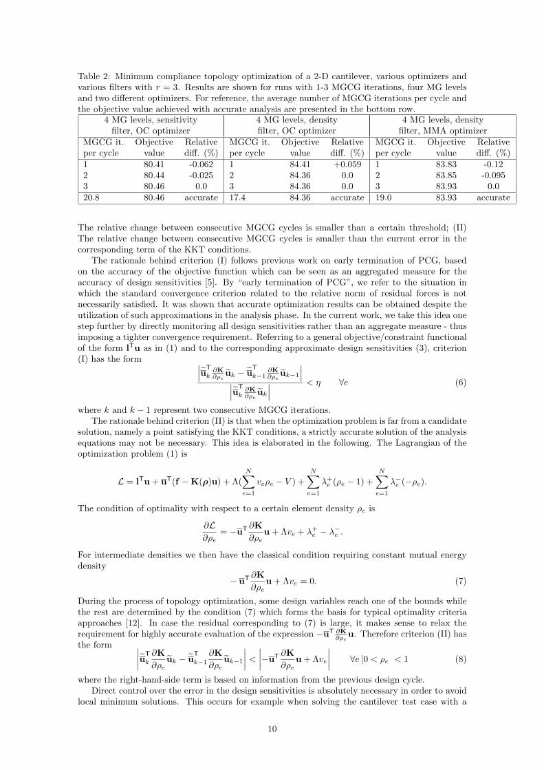
Table 2: Minimum compliance topology optimization of a 2-D cantilever, various optimizers andvarious filters with r = 3. Results are shown for runs with 1-3 MGCG iterations, four MG levelsand two different optimizers. For reference, the average number of MGCG iterations per cycle andthe objective value achieved with accurate analysis are presented in the bottom row.

4 MG levels, sensitivity 4 MG levels, density 4 MG levels, densityfilter, OC optimizer filter, OC optimizer filter, MMA optimizer

MGCG it. Objective Relative MGCG it. Objective Relative MGCG it. Objective Relativeper cycle value diff. (%) per cycle value diff. (%) per cycle value diff. (%)1 80.41 -0.062 1 84.41 +0.059 1 83.83 -0.122 80.44 -0.025 2 84.36 0.0 2 83.85 -0.0953 80.46 0.0 3 84.36 0.0 3 83.93 0.020.8 80.46 accurate 17.4 84.36 accurate 19.0 83.93 accurate

The relative change between consecutive MGCG cycles is smaller than a certain threshold; (II)The relative change between consecutive MGCG cycles is smaller than the current error in thecorresponding term of the KKT conditions.

The rationale behind criterion (I) follows previous work on early termination of PCG, basedon the accuracy of the objective function which can be seen as an aggregated measure for theaccuracy of design sensitivities [5]. By “early termination of PCG”, we refer to the situation inwhich the standard convergence criterion related to the relative norm of residual forces is notnecessarily satisfied. It was shown that accurate optimization results can be obtained despite theutilization of such approximations in the analysis phase. In the current work, we take this idea onestep further by directly monitoring all design sensitivities rather than an aggregate measure - thusimposing a tighter convergence requirement. Referring to a general objective/constraint functionalof the form lTu as in (1) and to the corresponding approximate design sensitivities (3), criterion(I) has the form ∣∣∣uT

k∂K∂ρe

uk − uT

k−1∂K∂ρe

uk−1

∣∣∣∣∣∣uT

k∂K∂ρe

uk

∣∣∣ < η ∀e (6)

where k and k − 1 represent two consecutive MGCG iterations.The rationale behind criterion (II) is that when the optimization problem is far from a candidate

solution, namely a point satisfying the KKT conditions, a strictly accurate solution of the analysisequations may not be necessary. This idea is elaborated in the following. The Lagrangian of theoptimization problem (1) is

L = lTu + uT(f −K(ρ)u) + Λ(

N∑e=1

veρe − V ) +

N∑e=1

λ+e (ρe − 1) +

N∑e=1

λ−e (−ρe).

The condition of optimality with respect to a certain element density ρe is

∂L∂ρe

= −uT ∂K

∂ρeu + Λve + λ+e − λ−e .

For intermediate densities we then have the classical condition requiring constant mutual energydensity

− uT ∂K

∂ρeu + Λve = 0. (7)

During the process of topology optimization, some design variables reach one of the bounds whilethe rest are determined by the condition (7) which forms the basis for typical optimality criteriaapproaches [12]. In case the residual corresponding to (7) is large, it makes sense to relax therequirement for highly accurate evaluation of the expression −uT ∂K

∂ρeu. Therefore criterion (II) has

the form ∣∣∣∣uT

k

∂K

∂ρeuk − u

T

k−1∂K

∂ρeuk−1

∣∣∣∣ < ∣∣∣∣−uT ∂K

∂ρeu + Λve

∣∣∣∣ ∀e |0 < ρe < 1 (8)

where the right-hand-side term is based on information from the previous design cycle.Direct control over the error in the design sensitivities is absolutely necessary in order to avoid

local minimum solutions. This occurs for example when solving the cantilever test case with a

10

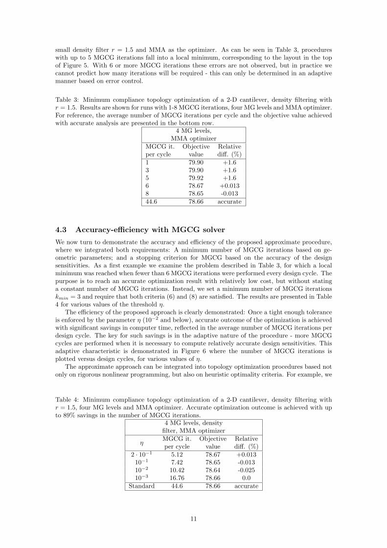
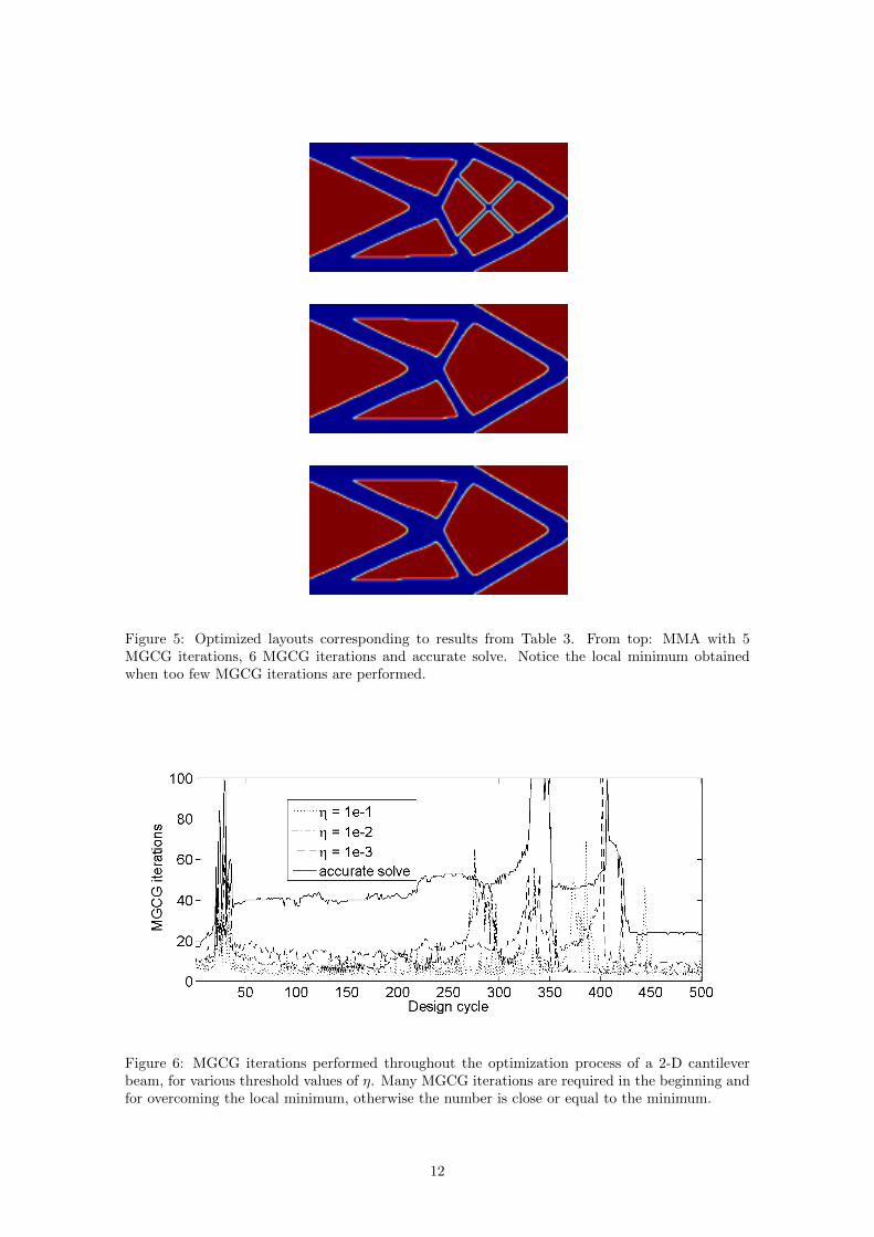
small density filter r = 1.5 and MMA as the optimizer. As can be seen in Table 3, procedureswith up to 5 MGCG iterations fall into a local minimum, corresponding to the layout in the topof Figure 5. With 6 or more MGCG iterations these errors are not observed, but in practice wecannot predict how many iterations will be required - this can only be determined in an adaptivemanner based on error control.

Table 3: Minimum compliance topology optimization of a 2-D cantilever, density filtering withr = 1.5. Results are shown for runs with 1-8 MGCG iterations, four MG levels and MMA optimizer.For reference, the average number of MGCG iterations per cycle and the objective value achievedwith accurate analysis are presented in the bottom row.

4 MG levels,MMA optimizer

MGCG it. Objective Relativeper cycle value diff. (%)1 79.90 +1.63 79.90 +1.65 79.92 +1.66 78.67 +0.0138 78.65 -0.01344.6 78.66 accurate

4.3 Accuracy-efficiency with MGCG solver

We now turn to demonstrate the accuracy and efficiency of the proposed approximate procedure,where we integrated both requirements: A minimum number of MGCG iterations based on ge-ometric parameters; and a stopping criterion for MGCG based on the accuracy of the designsensitivities. As a first example we examine the problem described in Table 3, for which a localminimum was reached when fewer than 6 MGCG iterations were performed every design cycle. Thepurpose is to reach an accurate optimization result with relatively low cost, but without statinga constant number of MGCG iterations. Instead, we set a minimum number of MGCG iterationskmin = 3 and require that both criteria (6) and (8) are satisfied. The results are presented in Table4 for various values of the threshold η.

The efficiency of the proposed approach is clearly demonstrated: Once a tight enough toleranceis enforced by the parameter η (10−2 and below), accurate outcome of the optimization is achievedwith significant savings in computer time, reflected in the average number of MGCG iterations perdesign cycle. The key for such savings is in the adaptive nature of the procedure - more MGCGcycles are performed when it is necessary to compute relatively accurate design sensitivities. Thisadaptive characteristic is demonstrated in Figure 6 where the number of MGCG iterations isplotted versus design cycles, for various values of η.

The approximate approach can be integrated into topology optimization procedures based notonly on rigorous nonlinear programming, but also on heuristic optimality criteria. For example, we

Table 4: Minimum compliance topology optimization of a 2-D cantilever, density filtering withr = 1.5, four MG levels and MMA optimizer. Accurate optimization outcome is achieved with upto 89% savings in the number of MGCG iterations.

4 MG levels, densityfilter, MMA optimizer

ηMGCG it. Objective Relativeper cycle value diff. (%)

2 · 10−1 5.12 78.67 +0.01310−1 7.42 78.65 -0.01310−2 10.42 78.64 -0.02510−3 16.76 78.66 0.0

Standard 44.6 78.66 accurate

11

Figure 5: Optimized layouts corresponding to results from Table 3. From top: MMA with 5MGCG iterations, 6 MGCG iterations and accurate solve. Notice the local minimum obtainedwhen too few MGCG iterations are performed.

Figure 6: MGCG iterations performed throughout the optimization process of a 2-D cantileverbeam, for various threshold values of η. Many MGCG iterations are required in the beginning andfor overcoming the local minimum, otherwise the number is close or equal to the minimum.

12

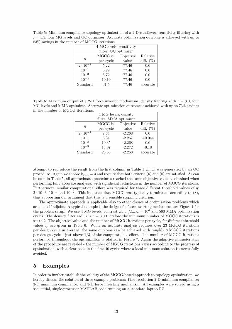
Table 5: Minimum compliance topology optimization of a 2-D cantilever, sensitivity filtering withr = 1.5, four MG levels and OC optimizer. Accurate optimization outcome is achieved with up to83% savings in the number of MGCG iterations.

4 MG levels, sensitivityfilter, OC optimizer

ηMGCG it. Objective Relativeper cycle value diff. (%)

2 · 10−1 5.22 77.46 0.010−1 5.29 77.46 0.010−2 5.72 77.46 0.010−3 10.10 77.46 0.0

Standard 31.5 77.46 accurate

Table 6: Maximum output of a 2-D force inverter mechanism, density filtering with r = 3.0, fourMG levels and MMA optimizer. Accurate optimization outcome is achieved with up to 73% savingsin the number of MGCG iterations.

4 MG levels, densityfilter, MMA optimizer

ηMGCG it. Objective Relativeper cycle value diff. (%)

2 · 10−1 7.34 -2.268 0.010−1 6.34 -2.267 +0.04410−2 10.35 -2.268 0.010−3 13.97 -2.272 -0.18

Standard 23.56 -2.268 accurate

attempt to reproduce the result from the first column in Table 1 which was generated by an OCprocedure. Again we choose kmin = 3 and require that both criteria (6) and (8) are satisfied. As canbe seen in Table 5, all approximate procedures reached the same objective value as obtained whenperforming fully accurate analyses, with significant reductions in the number of MGCG iterations.Furthermore, similar computational effort was required for three different threshold values of η:2 · 10−1, 10−1 and 10−2. This indicates that MGCG was typically terminated according to (8),thus supporting our argument that this is a sensible stopping criterion.

The approximate approach is applicable also to other classes of optimization problems whichare not self-adjoint. A typical example is the design of a force inverting mechanism, see Figure 1 forthe problem setup. We use 4 MG levels, contrast Emax/Emin = 106 and 500 MMA optimizationcycles. The density filter radius is r = 3.0 therefore the minimum number of MGCG iterations isset to 2. The objective value and the number of MGCG iterations per cycle, for different thresholdvalues η, are given in Table 6. While an accurate analysis requires over 23 MGCG iterationsper design cycle in average, the same outcome can be achieved with roughly 8 MGCG iterationsper design cycle - just above 1/3 of the computational effort. The number of MGCG iterationsperformed throughout the optimization is plotted in Figure 7. Again the adaptive characteristicsof the procedure are revealed - the number of MGCG iterations varies according to the progress ofoptimization, with a clear peak in the first 40 cycles where a local minimum solution is successfullyavoided.

5 Examples

In order to further establish the validity of the MGCG-based approach to topology optimization, wehereby discuss the solution of three example problems: Fine-resolution 2-D minimum compliance;3-D minimum compliance; and 3-D force inverting mechanism. All examples were solved using asequential, single-processor MATLAB code running on a standard laptop PC.

13

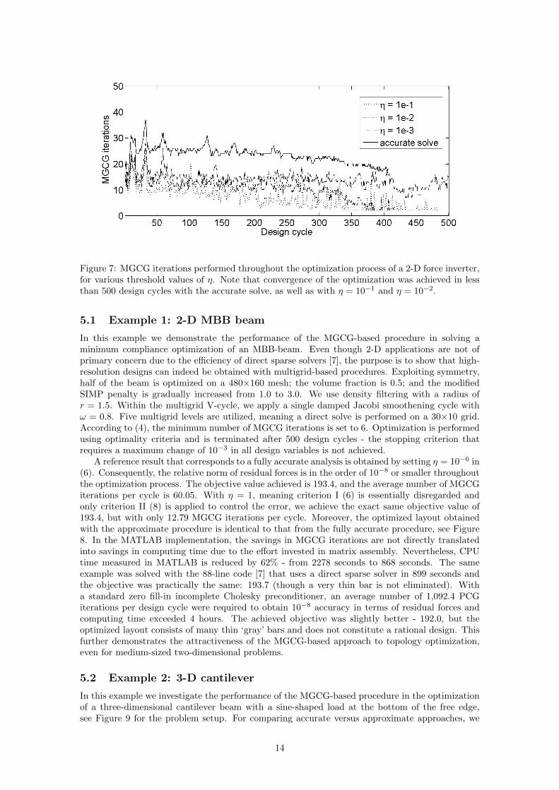
Figure 7: MGCG iterations performed throughout the optimization process of a 2-D force inverter,for various threshold values of η. Note that convergence of the optimization was achieved in lessthan 500 design cycles with the accurate solve, as well as with η = 10−1 and η = 10−2.

5.1 Example 1: 2-D MBB beam

In this example we demonstrate the performance of the MGCG-based procedure in solving aminimum compliance optimization of an MBB-beam. Even though 2-D applications are not ofprimary concern due to the efficiency of direct sparse solvers [7], the purpose is to show that high-resolution designs can indeed be obtained with multigrid-based procedures. Exploiting symmetry,half of the beam is optimized on a 480×160 mesh; the volume fraction is 0.5; and the modifiedSIMP penalty is gradually increased from 1.0 to 3.0. We use density filtering with a radius ofr = 1.5. Within the multigrid V-cycle, we apply a single damped Jacobi smoothening cycle withω = 0.8. Five multigrid levels are utilized, meaning a direct solve is performed on a 30×10 grid.According to (4), the minimum number of MGCG iterations is set to 6. Optimization is performedusing optimality criteria and is terminated after 500 design cycles - the stopping criterion thatrequires a maximum change of 10−3 in all design variables is not achieved.

A reference result that corresponds to a fully accurate analysis is obtained by setting η = 10−6 in(6). Consequently, the relative norm of residual forces is in the order of 10−8 or smaller throughoutthe optimization process. The objective value achieved is 193.4, and the average number of MGCGiterations per cycle is 60.05. With η = 1, meaning criterion I (6) is essentially disregarded andonly criterion II (8) is applied to control the error, we achieve the exact same objective value of193.4, but with only 12.79 MGCG iterations per cycle. Moreover, the optimized layout obtainedwith the approximate procedure is identical to that from the fully accurate procedure, see Figure8. In the MATLAB implementation, the savings in MGCG iterations are not directly translatedinto savings in computing time due to the effort invested in matrix assembly. Nevertheless, CPUtime measured in MATLAB is reduced by 62% - from 2278 seconds to 868 seconds. The sameexample was solved with the 88-line code [7] that uses a direct sparse solver in 899 seconds andthe objective was practically the same: 193.7 (though a very thin bar is not eliminated). Witha standard zero fill-in incomplete Cholesky preconditioner, an average number of 1,092.4 PCGiterations per design cycle were required to obtain 10−8 accuracy in terms of residual forces andcomputing time exceeded 4 hours. The achieved objective was slightly better - 192.0, but theoptimized layout consists of many thin ‘gray’ bars and does not constitute a rational design. Thisfurther demonstrates the attractiveness of the MGCG-based approach to topology optimization,even for medium-sized two-dimensional problems.

5.2 Example 2: 3-D cantilever

In this example we investigate the performance of the MGCG-based procedure in the optimizationof a three-dimensional cantilever beam with a sine-shaped load at the bottom of the free edge,see Figure 9 for the problem setup. For comparing accurate versus approximate approaches, we

14

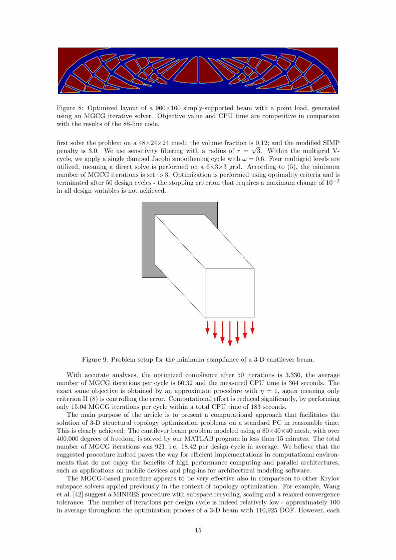
Figure 8: Optimized layout of a 960×160 simply-supported beam with a point load, generatedusing an MGCG iterative solver. Objective value and CPU time are competitive in comparisonwith the results of the 88-line code.

first solve the problem on a 48×24×24 mesh; the volume fraction is 0.12; and the modified SIMPpenalty is 3.0. We use sensitivity filtering with a radius of r =

√3. Within the multigrid V-

cycle, we apply a single damped Jacobi smoothening cycle with ω = 0.6. Four multigrid levels areutilized, meaning a direct solve is performed on a 6×3×3 grid. According to (5), the minimumnumber of MGCG iterations is set to 3. Optimization is performed using optimality criteria and isterminated after 50 design cycles - the stopping criterion that requires a maximum change of 10−2

in all design variables is not achieved.

Figure 9: Problem setup for the minimum compliance of a 3-D cantilever beam.

With accurate analyses, the optimized compliance after 50 iterations is 3,330, the averagenumber of MGCG iterations per cycle is 60.32 and the measured CPU time is 364 seconds. Theexact same objective is obtained by an approximate procedure with η = 1, again meaning onlycriterion II (8) is controlling the error. Computational effort is reduced significantly, by performingonly 15.04 MGCG iterations per cycle within a total CPU time of 183 seconds.

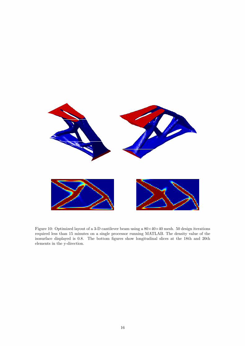
The main purpose of the article is to present a computational approach that facilitates thesolution of 3-D structural topology optimization problems on a standard PC in reasonable time.This is clearly achieved: The cantilever beam problem modeled using a 80×40×40 mesh, with over400,000 degrees of freedom, is solved by our MATLAB program in less than 15 minutes. The totalnumber of MGCG iterations was 921, i.e. 18.42 per design cycle in average. We believe that thesuggested procedure indeed paves the way for efficient implementations in computational environ-ments that do not enjoy the benefits of high performance computing and parallel architectures,such as applications on mobile devices and plug-ins for architectural modeling software.

The MGCG-based procedure appears to be very effective also in comparison to other Krylovsubspace solvers applied previously in the context of topology optimization. For example, Wanget al. [42] suggest a MINRES procedure with subspace recycling, scaling and a relaxed convergencetolerance. The number of iterations per design cycle is indeed relatively low - approximately 100in average throughout the optimization process of a 3-D beam with 110,925 DOF. However, each

15

Figure 10: Optimized layout of a 3-D cantilever beam using a 80×40×40 mesh. 50 design iterationsrequired less than 15 minutes on a single processor running MATLAB. The density value of theisosurface displayed is 0.8. The bottom figures show longitudinal slices at the 18th and 20thelements in the y-direction.

16

linear solve took 50.5 seconds in average on a single processor with similar properties to the oneused in the current study. For comparison, the current MGCG-based procedure requires 3.66seconds per design cycle of a 3-D beam with 91,875 DOF. Even if we assume that advances incomputer hardware are responsible for part of the gap, still the current results imply significantimprovements. Another reference result is the utilization of FETI-DP [20] in parallel topologyoptimization as reported by Evgrafov et al. [19]. When optimizing a 3-D beam with roughly1,000,000 DOF, 300 CG iterations were required in each design cycle, taking approximately 85seconds on 96 processors. Again, it appears that MGCG can be much more efficient: In theexample above with 400,000 DOF, only 18.42 MGCG iterations were performed every design cycleand the time required was 17.86 seconds on a single processor. Assuming linear increase in timewith respect to problem size, as expected in multigrid procedures, implies significant reduction incomputing time also in comparison to the FETI-DP approach.

5.3 Example 3: 3-D force inverter

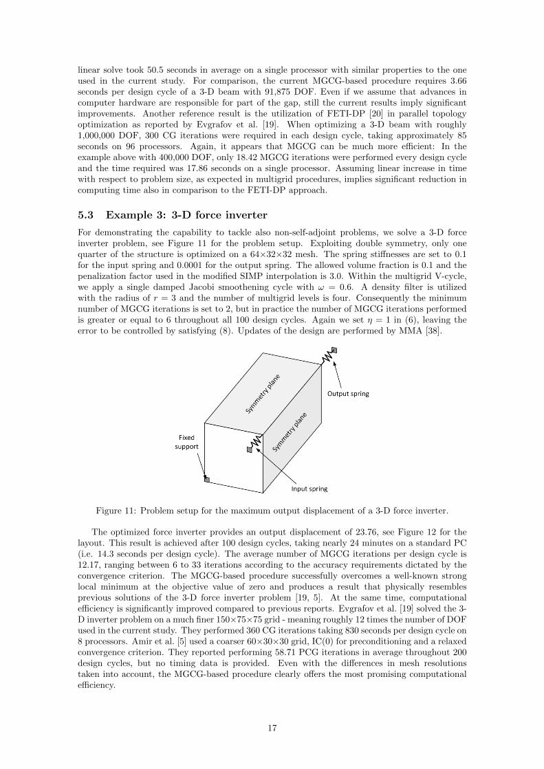
For demonstrating the capability to tackle also non-self-adjoint problems, we solve a 3-D forceinverter problem, see Figure 11 for the problem setup. Exploiting double symmetry, only onequarter of the structure is optimized on a 64×32×32 mesh. The spring stiffnesses are set to 0.1for the input spring and 0.0001 for the output spring. The allowed volume fraction is 0.1 and thepenalization factor used in the modified SIMP interpolation is 3.0. Within the multigrid V-cycle,we apply a single damped Jacobi smoothening cycle with ω = 0.6. A density filter is utilizedwith the radius of r = 3 and the number of multigrid levels is four. Consequently the minimumnumber of MGCG iterations is set to 2, but in practice the number of MGCG iterations performedis greater or equal to 6 throughout all 100 design cycles. Again we set η = 1 in (6), leaving theerror to be controlled by satisfying (8). Updates of the design are performed by MMA [38].

Figure 11: Problem setup for the maximum output displacement of a 3-D force inverter.

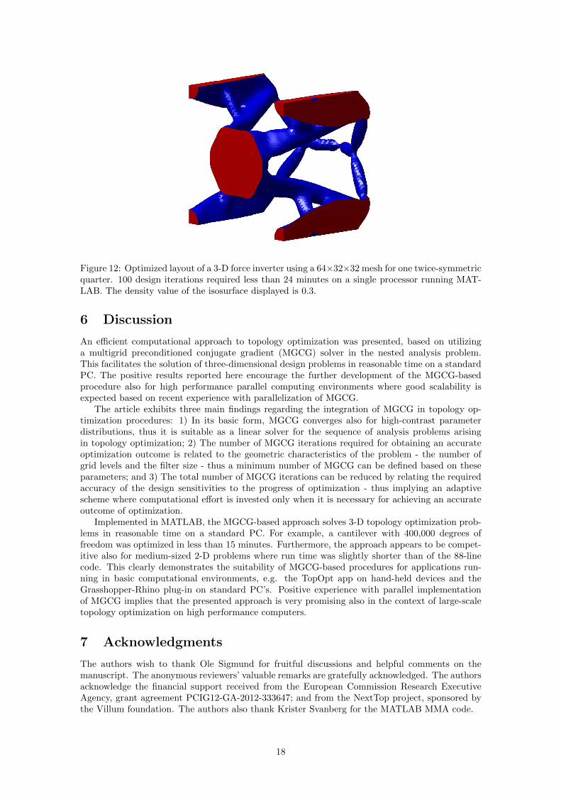
The optimized force inverter provides an output displacement of 23.76, see Figure 12 for thelayout. This result is achieved after 100 design cycles, taking nearly 24 minutes on a standard PC(i.e. 14.3 seconds per design cycle). The average number of MGCG iterations per design cycle is12.17, ranging between 6 to 33 iterations according to the accuracy requirements dictated by theconvergence criterion. The MGCG-based procedure successfully overcomes a well-known stronglocal minimum at the objective value of zero and produces a result that physically resemblesprevious solutions of the 3-D force inverter problem [19, 5]. At the same time, computationalefficiency is significantly improved compared to previous reports. Evgrafov et al. [19] solved the 3-D inverter problem on a much finer 150×75×75 grid - meaning roughly 12 times the number of DOFused in the current study. They performed 360 CG iterations taking 830 seconds per design cycle on8 processors. Amir et al. [5] used a coarser 60×30×30 grid, IC(0) for preconditioning and a relaxedconvergence criterion. They reported performing 58.71 PCG iterations in average throughout 200design cycles, but no timing data is provided. Even with the differences in mesh resolutionstaken into account, the MGCG-based procedure clearly offers the most promising computationalefficiency.

17

Figure 12: Optimized layout of a 3-D force inverter using a 64×32×32 mesh for one twice-symmetricquarter. 100 design iterations required less than 24 minutes on a single processor running MAT-LAB. The density value of the isosurface displayed is 0.3.

6 Discussion

An efficient computational approach to topology optimization was presented, based on utilizinga multigrid preconditioned conjugate gradient (MGCG) solver in the nested analysis problem.This facilitates the solution of three-dimensional design problems in reasonable time on a standardPC. The positive results reported here encourage the further development of the MGCG-basedprocedure also for high performance parallel computing environments where good scalability isexpected based on recent experience with parallelization of MGCG.

The article exhibits three main findings regarding the integration of MGCG in topology op-timization procedures: 1) In its basic form, MGCG converges also for high-contrast parameterdistributions, thus it is suitable as a linear solver for the sequence of analysis problems arisingin topology optimization; 2) The number of MGCG iterations required for obtaining an accurateoptimization outcome is related to the geometric characteristics of the problem - the number ofgrid levels and the filter size - thus a minimum number of MGCG can be defined based on theseparameters; and 3) The total number of MGCG iterations can be reduced by relating the requiredaccuracy of the design sensitivities to the progress of optimization - thus implying an adaptivescheme where computational effort is invested only when it is necessary for achieving an accurateoutcome of optimization.

Implemented in MATLAB, the MGCG-based approach solves 3-D topology optimization prob-lems in reasonable time on a standard PC. For example, a cantilever with 400,000 degrees offreedom was optimized in less than 15 minutes. Furthermore, the approach appears to be compet-itive also for medium-sized 2-D problems where run time was slightly shorter than of the 88-linecode. This clearly demonstrates the suitability of MGCG-based procedures for applications run-ning in basic computational environments, e.g. the TopOpt app on hand-held devices and theGrasshopper-Rhino plug-in on standard PC’s. Positive experience with parallel implementationof MGCG implies that the presented approach is very promising also in the context of large-scaletopology optimization on high performance computers.

7 Acknowledgments

The authors wish to thank Ole Sigmund for fruitful discussions and helpful comments on themanuscript. The anonymous reviewers’ valuable remarks are gratefully acknowledged. The authorsacknowledge the financial support received from the European Commission Research ExecutiveAgency, grant agreement PCIG12-GA-2012-333647; and from the NextTop project, sponsored bythe Villum foundation. The authors also thank Krister Svanberg for the MATLAB MMA code.

18

References

[1] N. Aage and B. Lazarov. Parallel framework for topology optimization using the method ofmoving asymptotes. Structural and Multidisciplinary Optimization, 47(4):493–505, 2013. doi:10.1007/s00158-012-0869-2.

[2] N. Aage, M. Nobel-Jørgensen, C. S. Andreasen, and O. Sigmund. Interactive topology op-timization on hand-held devices. Structural and Multidisciplinary Optimization, 47(1):1–6,2013.

[3] O. Amir and O. Sigmund. On reducing computational effort in topology optimization: howfar can we go? Structural and Multidisciplinary Optimization, 44:25–29, 2011.

[4] O. Amir, M. P. Bendsøe, and O. Sigmund. Approximate reanalysis in topology optimization.International Journal for Numerical Methods in Engineering, 78:1474–1491, 2009.

[5] O. Amir, M. Stolpe, and O. Sigmund. Efficient use of iterative solvers in nested topologyoptimization. Structural and Multidisciplinary Optimization, 42:55–72, 2010.

[6] O. Amir, O. Sigmund, M. Schevenels, and B. Lazarov. Efficient reanalysis techniques forrobust topology optimization. Computer Methods in Applied Mechanics and Engineering,245-246:217–231, 2012.

[7] E. Andreassen, A. Clausen, M. Schevenels, B. S. Lazarov, and O. Sigmund. Efficient topologyoptimization in matlab using 88 lines of code. Structural and Multidisciplinary Optimization,43:1–16, 2011.

[8] S. F. Ashby and R. D. Falgout. A parallel multigrid preconditioned conjugate gradient al-gorithm for groundwater flow simulations. Nuclear Science and Engineering, 124:145–159,1996.

[9] A. Baker, R. Falgout, T. Gamblin, T. Kolev, M. Schulz, and U. Yang. Scaling algebraicmultigrid solvers: On the road to exascale. In C. Bischof, H.-G. Hegering, W. E. Nagel,and G. Wittum, editors, Competence in High Performance Computing 2010, pages 215–226.Springer Berlin Heidelberg, 2012.

[10] A. Baker, R. Falgout, T. Kolev, and U. Yang. Scaling hypre’s multigrid solvers to 100,000cores. In M. W. Berry, K. A. Gallivan, E. Gallopoulos, A. Grama, B. Philippe, Y. Saad, andF. Saied, editors, High-Performance Scientific Computing, pages 261–279. Springer London,2012. doi: 10.1007/978-1-4471-2437-5 13.

[11] M. P. Bendsøe. Optimal shape design as a material distribution problem. Structural Opti-mization, 1:193–202, 1989.

[12] M. P. Bendsøe and O. Sigmund. Topology Optimization - Theory, Methods and Applications.Springer, Berlin, 2003.

[13] M. Bogomolny. Topology optimization for free vibrations using combined approximations.International Journal for Numerical Methods in Engineering, 82(5):617–636, 2010. doi: 10.1002/nme.2778.

[14] B. Bourdin. Filters in topology optimization. International Journal for Numerical Methodsin Engineering, 50:2143–2158, 2001.

[15] J. H. Bramble, J. E. Pasciak, J. Wang, and J. Xu. Convergence estimates for multigridalgorithms without regularity assumptions. Mathematics of Computation, 57:23–45, 1991.

[16] T. E. Bruns and D. A. Tortorelli. Topology optimization of non-linear elastic structuresand compliant mechanisms. Computer Methods in Applied Mechanics and Engineering, 190:3443–3459, 2001.

[17] E. Chow, R. D. Falgout, J. J. Hu, R. S. Tuminaro, and U. M. Yang. A survey of parallelizationtechniques for multigrid solvers. In M. A. Heroux, P. Raghavan, and H. D. Simon, editors,Parallel Processing for Scientific Computing, chapter 10, pages 179–201. SIAM, 2006.

19

[18] T. A. Davis. Direct Methods for Sparse Linear System. SIAM, 2006.

[19] A. Evgrafov, C. J. Rupp, K. Maute, and M. L. Dunn. Large-scale parallel topology optimiza-tion using a dual-primal substructuring solver. Structural and Multidisciplinary Optimization,36:329–345, 2008.

[20] C. Farhat, M. Lesoinne, P. LeTallec, K. Pierson, and D. Rixen. FETI-DP: a dual–primalunified FETI method–part I: A faster alternative to the two-level FETI method. Internationaljournal for numerical methods in engineering, 50(7):1523–1544, 2001.

[21] J. K. Guest and L. C. Smith Genut. Reducing dimensionality in topology optimization usingadaptive design variable fields. International Journal for Numerical Methods in Engineering,81(8):1019–1045, 2010. doi: 10.1002/nme.2724.

[22] M. R. Hestenes and E. Stiefel. Methods of conjugate gradients for solving linear systems.Journal of Research of the National Bureau of Standards, 49(6):409–436, 1952.

[23] J. E. Kim, G.-W. Jang, and Y. Y. Kim. Adaptive multiscale wavelet-galerkin analysis forplane elasticity problems and its applications to multiscale topology design optimization.International journal of solids and structures, 40(23):6473–6496, 2003.

[24] S. Y. Kim, I. Y. Kim, and C. K. Mechefske. A new efficient convergence criterion for re-ducing computational expense in topology optimization: reducible design variable method.International Journal for Numerical Methods in Engineering, 90(6):752–783, 2012. doi:10.1002/nme.3343.

[25] Y. Y. Kim and G. H. Yoon. Multi-resolution multi-scale topology optimization-a newparadigm. International Journal of Solids and Structures, 37(39):5529–5559, 2000.

[26] B. S. Lazarov. Topology optimization using multiscale finite element method for high-contrastmedia. 2013. In review.

[27] B. Maar and V. Schulz. Interior point multigrid methods for topology optimization. Structuraland Multidisciplinary Optimization, 19:214–224, 2000.

[28] T. H. Nguyen, G. H. Paulino, J. Song, and C. H. Le. A computational paradigm for mul-tiresolution topology optimization (mtop). Structural and Multidisciplinary Optimization, 41:525–539, 2010. doi: 10.1007/s00158-009-0443-8.

[29] T. H. Nguyen, G. H. Paulino, J. Song, and C. H. Le. Improving multiresolution topologyoptimization via multiple discretizations. International Journal for Numerical Methods inEngineering, 92(6):507–530, 2012. doi: 10.1002/nme.4344.

[30] T. A. Poulsen. Topology optimization in wavelet space. International Journal for NumericalMethods in Engineering, 53(3):567–582, 2002.

[31] Y. Saad. Iterative Methods for Sparse Linear Systems, Second Edition. SIAM, 2003.

[32] O. Sigmund. On the design of compliant mechanisms using topology optimization. MechanicsBased Design of Structures and Machines, 25:493–524, 1997.

[33] O. Sigmund and K. Maute. Sensitivity filtering from a continuum mechanics perspec-tive. Structural and Multidisciplinary Optimization, 46:471–475, 2012. doi: 10.1007/s00158-012-0814-4.

[34] O. Sigmund and S. Torquato. Design of materials with extreme thermal expansion using athree-phase topology optimization method. Journal of the Mechanics and Physics of Solids,45(6):1037–1067, 1997.

[35] R. Stainko. An adaptive multilevel approach to the minimal compliance problem in topologyoptimization. Communications in Numerical Methods in Engineering, 22(2):109–118, 2006.doi: 10.1002/cnm.800.

[36] R. Stainko. Advanced Multilevel Techniques to Topology Optimization. PhD thesis, JohannesKepler Universitat Linz, 2006.

20

[37] K. Suresh. Efficient generation of large-scale pareto-optimal topologies. Structural and Mul-tidisciplinary Optimization, 47:49–61, 2013. doi: 10.1007/s00158-012-0807-3.

[38] K. Svanberg. The method of moving asymptotes - a new method for structural optimization.International Journal for Numerical Methods in Engineering, 24:359–373, 1987.

[39] O. Tatebe and Y. Oyanagi. Efficient implementation of the multigrid preconditioned conjugategradient method on distributed memory machines. In Supercomputing’94. Proceedings, pages194–203. IEEE, 1994.

[40] U. Trottenberg, C. Oosterlee, and A. Schuller. Multigrid. Academic Press, 2001.

[41] P. S. Vassilevski. Multilevel Block Factorization Preconditioners: Matrix-based Analysis andAlgorithms for Solving Finite Element Equations. Springer, New York, 2008.

[42] S. Wang, E. de Sturler, and G. H. Paulino. Large-scale topology optimization using precondi-tioned Krylov subspace methods with recycling. International Journal for Numerical Methodsin Engineering, 69:2441–2468, 2007.

[43] S. Zhou and M. Y. Wang. Multimaterial structural topology optimization with a generalizedcahn-hilliard model of multiphase transition. Structural and Multidisciplinary Optimization,33:89–111, 2007. doi: 10.1007/s00158-006-0035-9.

[44] W. Zuo, T. Xu, H. Zhang, and T. Xu. Fast structural optimization with frequency con-straints by genetic algorithm using adaptive eigenvalue reanalysis methods. Structural andMultidisciplinary Optimization, 43:799–810, 2011. doi: 10.1007/s00158-010-0610-y.

21